Rigidity of compact Fuchsian manifolds with convex boundary
Abstract
A compact Fuchsian manifold with boundary is a hyperbolic 3-manifold homeomorphic to such that the boundary component is geodesic. We prove that a compact Fuchsian manifold with convex boundary is uniquely determined by the induced path metric on . We do not put further restrictions on the boundary except convexity.
1 Introduction
1.1 Rigidity of convex bodies in
Theorem 1.1.1.
Let and be convex bodies in the Euclidean space and be an isometry. Then extends to an isometry of .
By a convex body in we mean a compact convex set with non-empty interior. We endow its boundary with the induced path metric: the distance between two points is equal to the length of a shortest curve connecting them on the boundary. It is well-known that for convex bodies, even without the smoothness assumption on the boundary, a shortest curve of finite length always exists (although it might be not unique).
Theorem 1.1.1 was preceded by proofs under additional assumptions that the boundary is smooth (Cohn-Vossen [16] and Zhitomirsky [72] in the analytic class; Herglotz [30] in the -class; Sacksteder [56] in the -class) or that the boundary is polyhedral (Cauchy if the combinatorial structure is fixed; Alexandrov [3, 4] in the general case). Pogorelov managed to obtain a common generalization of smooth and polyhedral cases.
Theorem 1.1.1 is frequently stated as closed convex surfaces in are globally rigid. Here by a closed convex surface we mean the boundary of a convex body. Rigidity problems often go along with isometric realization problems. One of the most famous instances is the Weyl problem asking if every Riemannian metric on the 2-sphere with positive Gaussian curvature can be (smoothly) isometrically realized in . Such a realization should be a closed convex surface. Thus, the smooth instance of Theorem 1.1.1 says that the realization is unique. The Weyl problem was resolved positively in collective efforts of Weyl [71] (a proof outline); Lewy [40] (the analytic class); Nirenberg [49] (the -class); Heinz [29] (the -class). It was extended to the case of non-negative Gaussian curvature by Guan–Li [28] and Hong–Zuily [32].
Meanwhile Alexandrov started to investigate the induced boundary metrics on general convex bodies. He managed [3, 5] to find necessary and sufficient conditions on a metric on the 2-sphere to be realized as the boundary of a convex body. These are so-called CBB(0) metrics. The reader can find a similar definition of a CBB() metric in Subsection 2.1. First, Alexandrov resolved the problem in the polyhedral case, then he obtained a realization result in the general case by means of polyhedral approximation. About ten years later Pogorelov proved his general rigidity result. Besides, Pogorelov also proved [53] that a -smooth Riemannian metric with positive Gaussian curvature admits a -smooth realization for any . This allows to obtain a different resolution of the Weyl problem from Alexandrov–Pogorelov works. It is interesting to remark that in the smooth case the rigidity problem is commonly considered easier than the realization problem, but in the general case it seems to be on the contrary.
Pogorelov himself proposed two approaches to Theorem 1.1.1, both are quite lengthy and intricate. In both of them Pogorelov uses significantly the linear structure of . In the first approach Pogorelov supposes that there exist two convex bodies , and an isometry that does not extend to an ambient isometry. Then he considers a supplementary surface defined with the help of the radius functions of . He studies planar sections of the new surface and, with their help, constructs on the boundaries of initial bodies a pair of -isometric simple closed curves bounding regions that need to be intrinsically isometric, but have non-equal generalized Gaussian curvature. This can not happen because Alexandrov proved that the generalized Gaussian curvature is intrinsic (this is a generalization of the Gauss’s Theorema Egregium to non-smooth surfaces). In the second approach, from a violation of the global rigidity Pogorelov deduces a violation of the local rigidity and, finally, a violation of the infinitesimal rigidity. He shows that this is not possible. We refer also to the survey of Sen’kin [61] for a discussion of Pogorelov’s proof and some further developments.
A natural problem is to quantify the rigidity in Theorem 1.1.1. In other words, one can ask: if the boundaries of , are sufficiently close in the intrinsic sense, how close are , themselves?
Definition 1.1.2.
Let be a homeomorphism between metric spaces. It is called an -isometry if for any
Problem 1.1.3 (The Cohn-Vossen problem [17, 69]).
Let , be convex bodies in , and be an -isometry. Do there exist a continuous function such that and a constant that depends only on global geometry of (e.g., its diameter) such that extends to a -isometry between and ?
Volkov claimed a solution to this problem in [69] (for ). An English translation was published as an appendix to the book [4]. Volkov’s proof is completely unrelated to both Pogorelov’s approaches, so, in particular, it gives a third way to prove Theorem 1.1.1. The paper [69] is highly innovative without any doubts. However, we have some concerns on it. There are some gaps that can be bridged after some non-trivial work. But more important, some essential arguments are written in a very brief and cryptic way making them hard to interpret. We describe our remarks on Volkov’s paper in Appendix A.
The present paper can be considered as a revival of paper [69] with an application to a rigidity problem for a family of hyperbolic 3-manifolds. We use many important ideas from [69] and its influence on this paper can not be discounted. But in some steps of the proof we have to choose a different road due to our inability to understand some parts of [69]. We think that a proof of Theorem 1.1.1 can be obtained by the means of the present manuscript, but they are insufficient to resolve Problem 1.1.3.
1.2 Rigidity of hyperbolic 3-manifolds
The second source of our motivation comes from the importance of hyperbolic 3-manifolds to 3-dimensional topology highlighted in breakthrough works of Thurston. We quickly recall that Thurston proposed the geometrization program to understand the topology of 3-manifolds: each 3-manifold can be canonically decomposed into pieces and each piece can be endowed with one of eight canonical geometries (see, e.g. [66, 67]). The geometrization program was deeply developed by plenty of researchers with its notable culmination in the works of Perelman. Among all 3-manifolds admitting canonical geometries, hyperbolic manifolds constitute the largest and the most mysterious class. Hence, much of the efforts of researchers were directed toward developing a deeper understanding of hyperbolic 3-manifolds.
One of the foundational properties of hyperbolic manifolds (closed or of finite volume) in dimensions starting from 3 is their rigidity. It was first proved by Mostow [48] for closed manifolds and was extended to the case of finite volume by Prasad [54].
Theorem 1.2.1.
Let be a homotopy equivalence between two hyperbolic -dimensional manifolds of finite volume (without boundary) and . Then is homotopic to an isometry.
One can loosely rephrase it by saying that the geometry of a hyperbolic manifold of finite volume without boundary in dimension at least 3 is completely determined by its topology. It is natural to investigate hyperbolic manifolds with boundary in a similar vein. From the Pogorelov rigidity and the Mostow rigidity one can expect that in the case of convex boundary, the geometry of a hyperbolic 3-manifold should be determined by the topology and the induced boundary metric. In the topologically simplest case when the manifold is the 3-ball a proof was outlined by Pogorelov [53] and finalized by Milka [45] (see the introduction of [45] for the discussion of proof attempts).
Theorem 1.2.2.
Let and be convex bodies in and be an isometry. Then extends to an isometry of .
The proof of Theorem 1.2.2 appears to be quite different from the proof of Theorem 1.1.1 given by Pogorelov, probably, because the latter seems to be quite specific to . For the hyperbolic case Pogorelov proposed a map that produces a correspondence between pairs of convex surfaces in both spaces and allows to relate the rigidity problem in to the corresponding problem in . Pogorelov developed all necessary tools and completed the proof of rigidity in the spherical space, but the details of the proof in the hyperbolic space were furnished in further works, see [45].
Next, Schlenker [58] proved the rigidity of hyperbolic 3-manifolds with smooth strictly convex boundary. Here by strict convexity we mean that the shape operator is positive-definite for the outward choice of the unit normal field. By the Gauss equation this implies that the Gaussian curvature of the boundary is strictly greater than . We rephrase his result (the uniqueness part of Theorem 0.1 in [59]) as follows:
Theorem 1.2.3.
Let and be compact hyperbolic 3-manifolds with smooth strictly convex boundaries and be a homeomorphism such that its restriction to the boundary is isotopic to an isometry. Then is isotopic to an isometry.
Previously Labourie [38] proved the corresponding realization result: if the interior of a compact 3-manifold with non-empty boundary admits a cocompact hyperbolic metric, then each smooth metric with Gaussian curvature greater than on is induced by a hyperbolic metric on . Schlenker provided another proof of this in [58].
Due to Pogorelov’s global rigidity for general bodies, it is natural to expect that the smoothness and strict convexity assumptions are superfluous. One can conjecture
Conjecture 1.2.4.
Let and be compact hyperbolic 3-manifolds with convex boundaries and be a homeomorphism such that its restriction to the boundary is isotopic to an isometry. Then is isotopic to an isometry.
Here by convex boundary we mean that the boundary is locally modelled on convex subsets of .
The aim of the present paper is to prove this conjecture for a particular family of hyperbolic 3-manifolds with boundary.
Definition 1.2.5.
A compact Fuchsian manifold with boundary is a hyperbolic 3-manifold homeomorphic to , where is a closed oriented surface of genus , such that is geodesic.
In what follows we will omit the word “compact” assuming that this is always the case. We will refer to the boundary component as to the lower boundary and to the component as to the upper boundary, and denote them by and respectively, where is a Fuchsian manifold with boundary.
Fuchsian manifolds with boundary are considered as toy cases in the study of hyperbolic 3-manifolds with boundary, and the interest to them can be traced back to the works of Pogorelov [53, Section VI.12] and Gromov [26, Section 3.2.4]. In particular, Gromov proved the smooth realization result: every smooth metric on of Gaussian curvature is induced on the upper boundary of a Fuchsian manifold. He conjectured that this realization is unique.
We note that some authors use slightly different definition of a Fuchsian manifold with boundary: they require it to be homeomorphic to and to contain an embedded geodesic surface isotopic to . If we cut such a manifold along this surface, we obtain two Fuchsian manifolds in the sense of Definition 1.2.5. The rigidity of Fuchsian manifolds in the sense of the other definition is equivalent to the rigidity of Fuchsian manifolds from Definition 1.2.5 with respect to the induced metric on the upper boundary. We find it more convenient to work in the setting of Definition 1.2.5.
In the case of polyhedral Fuchsian manifolds Fillastre [18] proved
Theorem 1.2.6.
Let and be two Fuchsian manifolds with convex polyhedral boundaries and be an isometry between the upper boundaries. Then extends to an isometry between and .
In the case of smooth boundary the same result follows from Theorem 1.2.3 by the doubling construction.
Our main result is
Theorem A.
Let and be two Fuchsian manifolds with convex boundaries and be an isometry between the upper boundaries. Then extends to an isometry between and .
Corollary 1.2.7.
Let and be compact hyperbolic 3-manifolds with convex boundaries such that are homeomorphic to and contain geodesic surfaces isotopic to . Let be a homeomorphism such that its restriction to the boundary is isotopic to an isometry. Then is isotopic to an isometry.
This seems to be the first known rigidity result for general boundary metrics and manifolds more complicated than the ball.
1.3 Related work
As we already mentioned, our proof of Theorem A follows the ideas of Volkov. It proceeds by means of polyhedral approximation. However, in order to prove the rigidity by approximation, the rigidity in the polyhedral case is insufficient and one needs to obtain a kind of stability. Assume, e.g., that we have two convex bodies in that are not ambiently isometric, but have isometric boundaries. We can approximate them by polyhedra. In this way we can obtain two polyhedra that are not close modulo ambient isometries, but have arbitrarily close boundaries. One needs to prove that this can not happen. Volkov’s main insight was that this can be achieved by deforming polyhedra through polyhedra with cone-singularities in the interior and by controlling the process with the help of discrete curvature.
It seems that Volkov’s PhD thesis from 1955, recently published as [70], was the first place where cone-3-manifolds and their discrete curvature was considered. He provided there a variational proof of Alexandrov’s realization and rigidity theorem on Euclidean polyhedra. Volkov also produced a similar proof in the case of so-called convex polyhedral caps [68]. One can find an English translation in the appendix to the book [4].
Now we describe some other works that were invaluably impacted by Volkov’s ideas.
In [8] Bobenko and Izmestiev elaborated the ideas of Volkov further and gave another variational proof of the Alexandrov theorem. Based on their work Sechelmann developed [60] a computer program that constructs the polyhedron realizing a given Euclidean cone-metric. This resolved a long-standing problem (original Alexandrov’s proof was non-constructive). Izmestiev [34] also gave a new proof of the realization and rigidity of convex polyhedral caps, which provides a simple introduction to the approach. An investigation of convex polyhedral caps in the Minkowski space was done by Milka [46] in a way very similar to Volkov. In [21], [22] Fillastre and Izmestiev used these techniques for hyperbolic and spherical cone-metrics on the torus (realizing them in some hyperbolic and de Sitter manifolds respectively).
Alexandrov also proved a realization and rigidity result for convex polyhedra in . One might also consider (non-compact) polyhedra in with ideal vertices on the boundary at infinity of and with hyper-ideal vertices outside of it (in the projective model). Fillastre [19] proved an Alexandrov-type result for generalized Fuchsian polyhedra with vertices of these types. In [55] we investigated ideal Fuchsian polyhedra with the help of cone-manifolds and the discrete curvature. This is of particular interest due to its connection to discrete conformality. See more details, e.g., in [9, 27, 63, 55].
The realization counterpart to Theorem A comes from the work of Slutskiy [62]. He considered compact quasi-Fuchsian manifolds with convex boundary. They are also homeomorphic to , but the condition on the geodesic boundary is not imposed. The induced metric on a convex surface in a hyperbolic 3-manifold is CBB(). Slutskiy proved that for any pair of CBB() metrics on there exists a compact quasi-Fuchsian manifold with convex boundary realizing them. He used a smooth approximation and the smooth realization result of Labourie–Schlenker mentioned above. If one replaces the latter by the above mentioned smooth Fuchsian realization of Gromov, then one can obtain the general convex Fuchsian realization result without any difficulties. A similar realization result for CBB() metrics on the torus was obtained in [23].
A related and very active research area is the convex realization of metrics and their rigidity in Lorenzian space-forms. We refer to [57, 39, 20, 25, 14, 37, 65] for works in this direction.
In 70s cone-3-manifolds were rediscovered by Thurston who proposed to use them in order to describe deformations of hyperbolic structures. He demonstrated their usability in his proof of the hyperbolic Dehn filling theorem [66, Chapter 4]. Hyperbolic cone-3-manifolds were used heavily by Thurston’s school of 3-dimensional topology. We refer to [10, 31, 12] as just to few examples.
Mostow’s rigidity was also generalized to open hyperbolic 3-manifolds. By an open manifold we mean a non-compact connected 3-manifold without boundary. A subset of a hyperbolic manifold is called totally convex if contains every geodesic segment between any two points of . The convex core of a hyperbolic 3-manifold is the intersection of all closed totally convex subsets of . It is non-empty except for a specific family of examples. If is closed or is open, but has finite volume, then its convex core is itself.
The convex core is an important tool to investigate open hyperbolic 3-manifolds. An open hyperbolic 3-manifold is called cocompact if its convex core is compact. It is called geometrically finite if the convex core has finite volume. A geometrically finite hyperbolic-3-manifold can be naturally compactified and its boundary at infinity can be endowed with a conformal structure. Marden’s rigidity theorem [43] (based on the previous works of Ahlfors, Bers, Kra and Maskit) states that the geometry of a geometrically finite hyperbolic 3-manifold is completely determined by its topology and the conformal structure at infinity. To cover a more general case of all open hyperbolic 3-manifolds with finitely generated fundamental group one needs additional invariants called ending laminations. This was established in [47, 11].
1.4 Further work directions
A good direction of further research is Conjecture 1.2.4. In particular, after Fuchsian manifolds one may attempt to prove it for compact quasi-Fuchsian manifolds with convex boundary that were defined above. In this case we have to prescribe the metric on both boundary components. Fuchsian manifolds exhibit a warped product geometry, which quasi-Fuchsian manifolds lack. While remaining topologically still simple, quasi-Fuchsian manifolds already contain all geometric difficulties that appear when we try to proceed further from the Fuchsian case. It might happen that there are not much difficulties to extend the solution from the quasi-Fuchsian case to a more general topological case.
A nice application of Conjecture 1.2.4 should be another way to determine the geometry of open hyperbolic 3-manifolds. A long standing conjecture is
Conjecture 1.4.1.
The geometry of a geometrically finite hyperbolic 3-manifold is completely determined by the topology and the induced path metric on the boundary of its convex core.
The induced metric on the boundary of the convex core is totally hyperbolic, i.e., locally isometric to the hyperbolic plane. However, it is embedded in a non-smooth way and is bent along a geodesic lamination. This lamination together with an additional data (a transverse measure describing how much the surface is bent) is called a pleating lamination. The pleating lamination conjecture states that this data provides another way to determine the geometry of a geometrically finite hyperbolic 3-manifold. In some way it is dual to Conjecture 1.4.1.
Another important direction is to recover a proof of the Cohn-Vossen problem (Problem 1.1.3). As we mentioned in Section 1.1, the Cohn-Vossen problem was presumably solved by Volkov in [69], but we can not reconstruct some important steps of his proof. We are also unaware of any researchers that claim to understand this proof. One can also formulate the Cohn-Vossen problem, e.g., for Fuchsian manifolds:
Problem 1.4.2.
Let , be Fuchsian manifolds with convex boundaries, and be an -isometry. Does extend to a -isometry between and , where depends on global geometry of and is a continuous function satisfying ?
Acknowledgments. This work is a part of author’s doctoral thesis completed under the supervision of I. Izmestiev and the author is invaluably grateful to him for his constant attention and advice. The author is also very grateful to F. Fillastre and M. Ghomi for their helpful remarks.
Unfortunately, our paper is incredibly long so we tried to explain the links between sections as clear as possible. In Section 2 we go through preliminaries from metric geometry that we will use. Subsections 2.1–2.3 contain mostly standard material, although we make an emphasis on some specific details that will be important for us. In Subsection 2.4 we define trapezoids and prisms that are our elementary building blocks. With their help in Subsection 2.5 we define Fuchsian cone-manifolds that are the main heroes of our proof. In Subsection 2.6 we formulate some facts about them that are necessary for the proof and define the discrete curvature functional. In Section 3 we prove Theorem A modulo several tough lemmas concerning the stability of Fuchsian manifolds with polyhedral boundary. Next, in Section 4 we investigate thoroughly properties of Fuchsian cone-manifolds and of the discrete curvature that we use. Section 5 is devoted to the proofs of the main lemmas from Section 3. This section is the core of the paper.
2 Preliminaries
2.1 CBB() metrics
First, we briefly sketch the facts that we need about metrics with curvature bounded from below by in the sense of Alexandrov (CBB() for short). For a detailed exposition of CBB() metrics we refer to [15, 2]. Many properties of CBB() metrics on surfaces are similar to those of CBB(0) metrics, which are treated in details in [5] (with Chapter XII discussing also CBB() case).
Let be a connected orientable surface and be a complete intrinsic metric on . By intrinsic we mean that the distance between each pair of points is equal to the infimum of lengths of all rectifiable paths connecting them. Then this infimum is achieved: there exists a shortest path between any two points. This is a corollary of the Arzela–Ascoli theorem, see [15, Theorem 2.5.23].
Definition 2.1.1.
A geodesic is a rectifiable curve (possibly closed) that is locally distance minimizing.
Let , be two shortest paths in sharing an endpoint . Let be the point at distance from and be the point at distance from . Consider the hyperbolic triangle with side lengths , and and let be the angle opposite to the side of length .
Definition 2.1.2.
We say that is a CBB() metric on if is complete, intrinsic and for each there exists a neighbourhood such that the function is a nonincreasing function of and for every , emanating from , in the range , where the respective points belong to .
Definition 2.1.2 implies that the angle between and , which we define as , exists. Denote it by . In this way the angle could be defined between any two rectifiable curves sharing an endpoint, which are possibly not geodesics, but the angle might not exist.
It is important to note that the locality in Definition 2.1.2 can be dropped. Namely, for any three points the angle between shortest paths from to and to is at least the respective angle in the comparison triangle for , , , i.e., in the hyperbolic triangle with the side lengths , and . This is called the Toponogov globalization theorem, which was proved in the general case by Perelman. We refer to [15, Theorem 10.3.1].
For geodesics in CBB() spaces the non-overlapping property holds: if two geodesics have a segment in common, they can be covered by a larger geodesic. Sometimes we need a slightly stronger version: if two shortest paths have two points in common, then either these are their endpoints or they have a segment in common.
The shortest paths and emanating from a point divide a sufficiently small neighbourhood of into two sectors and . Let be shortest paths emanating from belonging to enumerated in the order from to . The angle is defined as the supremum of the sums over all finite collections of shortest paths from in . The smallest of , is equal to .
Definition 2.1.3.
The total angle of is equal to .
It does not depend on the choice of initial shortest paths , .
Definition 2.1.4.
A geodesic polygon is a submanifold of with piecewise geodesic boundary. It is called convex if there is a shortest path between any two of its points that belongs to the polygon.
It might be worth to note [5, Chapter II.6]:
Lemma 2.1.5.
Assume that is a compact CBB() surface. Then it admits a triangulation consisting of finitely many arbitrarily small convex geodesic triangles.
The area of a Borel set in is defined intrinsically as its Hausdorff measure. See [15, Chapters 1.7, 2.6].
We sketch the concept of the intrinsic curvature of a Borel set in .
For a point we define .
For a relatively open geodesic segment we define .
For an open geodesic triangle we define its curvature , where , , are the angles of .
These three types of sets are called primitive sets. An elementary set is a set that can be represented as a finite disjoint union of primitive sets. Then its curvature is the sum of the curvatures of these primitive sets. It does not depend on a representation. Then for a closed set in its curvature is defined as the infimum of the curvatures of its elementary supersets. For an open set its curvature is defined as the supremum of the curvatures of its closed subsets. This defines a Borel measure on : for the details we refer to [5, Chapters V, XII.1.6], [6, Chapter V] or [42].
However, we will mostly use the extrinsic curvature of a Borel set , namely,
For CBB() metrics it is non-negative: see [42]. In what follows we will omit the word extrinsic.
2.2 Hyperbolic convex bodies and duality
In this subsection we introduce basic facts from convex geometry in that we will use. Let be a closed convex set in with non-empty interior distinct from . Then its boundary is homeomorphic to an open subset of the sphere . First, we recall a fundamental result from convex geometry [44]:
Lemma 2.2.1 (The hyperbolic Busemann-Feller lemma).
Let and be the nearest points to them in . Then the hyperbolic distance between and is at most the hyperbolic distance between and .
Corollary 2.2.2.
Let be a rectifiable curve and be its nearest point projection to the boundary of . Then is rectifiable and its length is at most the length of .
Another well-known result is [5, Chapter XII]:
Lemma 2.2.3.
The boundary equipped with the induced path metric is CBB().
In particular, the curvature measure is defined for as in Section 2.1.
We will also use the hyperbolic – de Sitter duality. The de Sitter space is the space of oriented planes of . It is a Lorenzian manifold of constant curvature 1. More precisely, consider the hyperboloid model. Let be the 4-dimensional Minkowski space, i.e., equipped with the scalar product
We identify
and define the three-dimensional de Sitter space as
An oriented plane in is obtained as an intersection of with an oriented hyperplane in passing through the origin. Naturally, the unit normal to this hyperplane belongs to . There is a well-known duality between convex sets is and in . For a convex set we define the dual convex set as the set of all planes that do not intersect and are oriented outwards . We refer to [7, 24] for more details.
For each Borel set define its dual as the set of all planes tangent to and passing through points of . It is folklore that
However, we are unaware of any sources that prove this for non-smooth convex bodies, hence, we are providing a proof by ourselves.
We consider the case when is a convex body in , i.e. compact, convex and, as before, with non-empty interior. We follow the framework from [7]. Define
Assume without loss of generality that the point is in the interior of . Consider the cone in from the origin over . Define its dual cone
which is a convex cone containing the future cone of in its interior. Then
(see the details in [7]).
Define the Gauss map as the multivalued map sending a point on to the set of its outward unit normals. The set is space-like and comes with a well-defined area measure . This is proven in [7, Lemma 2.1].
Consider as the unit sphere in , let be the radial projection, i.e., a map that sends a point from the sphere to the endpoint on of the geodesic in the respective direction, and let be the function measuring the length of the this geodesic. We pull back to via and denote the obtained measure by . We also pull back the area measure to via and denote it by (note that it is not the same as in [7]).
We pull back our curvature measure to via and, abusing the notation, continue to denote it by .
Lemma 2.2.4 ([7], Proposition A.3).
There exists a sequence of convex bodies such that
(1) are smooth and strictly convex;
(2) converge to uniformly;
(3) converge to in the Hausdorff sense;
(4) the measures converge weakly to .
Now we are ready to prove
Lemma 2.2.5.
The measures and coincide. Thus, for each Borel set
Proof.
First, we claim that . Indeed, for let be the Gaussian curvature of and be the extrinsic curvature of , i.e., the determinant of the shape operator. The Gauss equation says that . Proposition 2.2.1 from [7] states that . We claim that also . Due to the Gauss equation, it is enough to show that . Take an open geodesic triangle . The Gauss-Bonnet theorem shows that . The measures of other elementary sets (geodesic arcs and points) are zero for smooth metrics. The proof of for any Borel set follows from the definition of and elementary properties of the Hausdorff measure . As , we get .
2.3 Cone-metrics and triangulations
Let be a closed oriented connected surface of genus . In this subsection we deal with hyperbolic cone-metrics on and their geodesic triangulations.
Definition 2.3.1.
A topological triangulation of is a finite vertex set and a collection of simple disjoint paths with endpoints in that cut into triangles with vertices in . Two topological triangulations with the same vertex set are equivalent if they are isotopic with respect to (so the edges are not allowed to pass through points of during the isotopy). A triangulation of is an equivalence class of topological triangulations with the same vertex set .
Note that this definition allows loops and multiple edges between two vertices. By we denote the set of vertices of and by we denote the set of edges of considered as isotopy classes of the respective paths.
Definition 2.3.2.
A hyperbolic cone-metric on is locally isometric to the metric of hyperbolic plane except finitely many points called conical points. At a conical point the metric is locally isometric to the metric of a hyperbolic cone with angle . The number is called the curvature of . We denote the set of conical points of by . A hyperbolic cone-metric is called convex if for every we have . Two metrics and are considered equivalent if and there is an isometry fixing and isotopic to identity with respect to .
Lemma 2.3.3 ([5], Chapter XII).
A convex hyperbolic cone-metric is CBB().
From now on we restrict ourselves almost only to the hyperbolic case and omit the word “hyperbolic” saying just cone-metrics (except in some special cases).
We note that on a cone-metric there can be multiple shortest paths between two points.
Definition 2.3.4.
A geodesic triangulation is a topological triangulation such that all edges are geodesics.
Definition 2.3.5.
Let be a triangulation of and be an intrinsic metric. We say that is realized by if there is a geodesic triangulation of in the class .
Note that if is a cone-metric, then we do not require in this definition neither nor the converse. We highlight that degenerated triangles are not allowed because the edges are defined up to isotopy with respect to . Sometimes when we write and the realization of is evident, then we mean the respective realization of . Similarly, when we consider a triangle of we frequently mean its realization in a metric.
We recall that a geodesic on a convex cone-metric can not pass through conical points. We will frequently need the following result, which follows from [36, Proposition 4]:
Lemma 2.3.6.
If is a cone-metric and , then there exists a triangulation realized by with . Moreover, any set of disjoint geodesic paths with vertices in can be extended to a geodesic triangulation.
In this case the metric is uniquely determined by and the edge lengths.
Definition 2.3.7.
Fix . By we denote the space of cone-metrics on with up to isometry isotopic to identity with respect to . By we denote the subspace of convex metrics. By we denote the subspace of strictly convex metrics with respect to , i.e., if and only if and is convex.
Definition 2.3.8.
Let be a triangulation of with . By we denote the set of cone-metrics realizing . Similarly we denote its subsets and .
Recall that if , then any triangulation of with vertices at has triangles and edges. The edge lengths map is injective. Abusing the notation, we frequently identify with its image under this map. Let us study its basic properties.
The set is an open polyhedron defined by the strict triangles inequalities for all triangles of . For every the total angle of defines an analytic function . Then is the subset of satisfying inequalities . It is a semi-analytic set.
If realizes two triangulations, then the transition maps are smooth. This endows with a smooth manifold structure. The set is its open subset.
Lemma 2.3.9.
Let . Define a 1-parameter family of cone-metrics by for each , where . Then is strictly monotonously decreasing for every .
Proof.
It is clear that all strict triangle inequalities are satisfied after multiplying by , therefore equations indeed define a metric . It remains to prove that if all edge lengths of a hyperbolic triangle are multiplied with the same factor , then its angles become strictly smaller.
Let be a triangle with the increased side lengths. Consider and such that and . It suffices to show that .
Now let be a Euclidean comparison triangle for and , be points such that and . Because of scaling we get . But because of elementary properties of comparison geometry (as the hyperbolic plane has curvature ). ∎
In what follows we will need the following corollary. Let , and be the open ball centered at of radius in . Define and .
Corollary 2.3.10.
For sufficiently small the set is connected.
Proof.
If , then the statement is clear as is an open set.
Assume that , but not in . As is semi-analytic, it is locally connected, i.e., for sufficiently small the set is connected. Now consider two points in . They can be joined by a path in . As is open, then for sufficiently close to 1, if we multiply all side lengths of by , then the new path still belongs to . On the other hand, belongs to by Lemma 2.3.9. It remains to connect the endpoints of the old path with the endpoints of the new one. ∎
2.4 Trapezoids and prisms
Trapezoids and prisms are the basic building blocks that we use to construct Fuchsian cone-manifolds in the next subsection.
Definition 2.4.1.
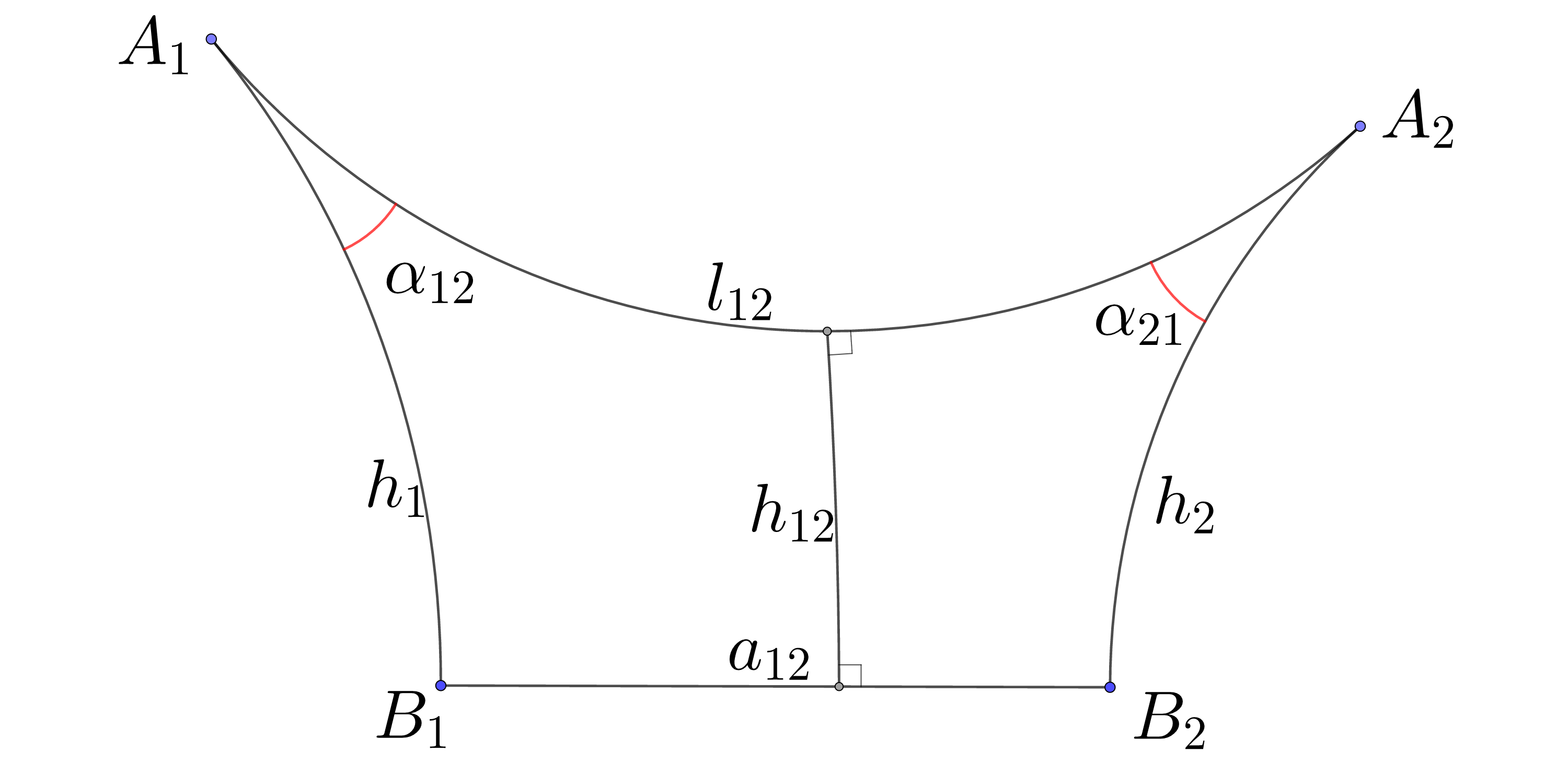
A trapezoid is the convex hull of a segment and its orthogonal projection to a line such that the segment does not intersect this line. It is called ultraparallel if the line is ultraparallel to the second line.
By denote the image of under the projection, . We refer to as to the upper edge, to as to the lower edge and to as to the lateral edges. The vertices are also called upper and are called lower. We denote by the length of , by the length of , by the length of , by and the angles at vertices and and by the distance from the line to the line in the case of an ultraparallel trapezoid. See Figure 1.
Definition 2.4.2.
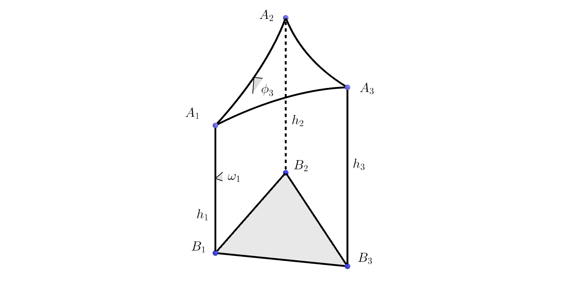
A prism is the convex hull of a triangle and its orthogonal projection to a plane such that the triangle does not intersect this plane. It is called ultraparallel if the plane is ultraparallel to the second plane.
Similarly to trapezoids, by we denote the image of under the projection, , and we distinguish edges and faces of a prism into upper, lower and lateral. The lateral faces of a prism are trapezoids. The dihedral angles of edges are equal . The dihedral angles of edges , and are denoted by , and respectively. The dihedral angle of an edge is denoted by . Other notation is inherited from trapezoids. See Figure 2.
We do not allow degenerations of the upper triangle, but we consider degenerate prisms with collinear , and , when the upper plane is orthogonal to the lower one. However, soon we will restrict ourselves only to ultraparallel ones, which do not degenerate.
Once can see a trapezoid (or a prism) as a triangle (respectively, a tetrahedron) with one hyperideal vertex dual to the lower edge (lower face).
The proof of next two lemmas is straightforward: see Thurston’s book [66, Chapter 2.6] for a general approach allowing to obtain these formulas.
Lemma 2.4.3 (The cosine laws).
For a trapezoid we have
Lemma 2.4.4 (The sine law).
For a trapezoid we have
In particular, for right-angled trapezoids we will use the following identities:
Corollary 2.4.5.
Assume that in a trapezoid . Then
A trapezoid or a prism is clearly determined uniquely by the lengths of the lower and lateral edges. From the cosine laws we also obtain that
Corollary 2.4.6.
A trapezoid or a prism is determined up to isometry by the lengths of the upper and lateral edges.
We end the section with a purely computational corollary of cosine/sine laws that will be used further.
Corollary 2.4.7.
For a trapezoid we have
2.5 Fuchsian cone-manifolds
Fuchsian cone-manifolds, which we introduce in this subsection, are the main tools of our proof and most of this paper is devoted to understanding their properties.
Definition 2.5.1.
A representable triple is a triple , where is a triangulation of with , and is a function on such that for every triangle of there exists a prism with the lengths of the upper edges defined by the side lengths of in and the lengths of the lateral edges determined by . We write as .
Definition 2.5.2.
Let be a representable triple. Take all prisms determined by , and and glue them isometrically according to . The resulting intrinsic metric space together with the canonical isometry from to the upper boundary provided by our construction, is called a marked Fuchsian cone-manifold with polyhedral boundary. In what follows we will mostly omit the words “marked” and “with polyhedral boundary” saying only a Fuchsian cone-manifold for short.
We say that a representable triple is a representation of and write . The upper and lower boundaries of are defined naturally. By definition, the upper boundary is identified with . We also say that the triangulation is compatible with . The function is called the height function of .
We say that an isometry between two Fuchsian cone-manifolds, where and with , is a marked isometry if its composition with the canonical isometries of , is an isometry between and isotopic to identity with respect to . We will consider Fuchsian cone-manifolds up to marked isometry.
For a Fuchsian cone-manifold and we denote by the sum of dihedral angles of the respective lateral edges in all prisms incident to in and define the particle curvature of in as . If all , then is a Fuchsian manifold with polyhedral boundary. We will also call it a polyhedral Fuchsian manifold for short. Let be a triangulation compatible with . For denote by its length in the metric , by its dihedral angle in and by the curvature of . A Fuchsian cone-manifold is called convex if the dihedral angles of all edges of are not greater than . Convex Fuchsian cone-manifolds are our main objects and we consider non-convex ones only sometimes in intermediate steps of proofs.
The upper boundary admits a canonical stratification as follows. The spherical link of a point at the boundary of a prism is the portion of the unit sphere in corresponding to the directions to . Now for a point we define naturally its spherical link as the gluing of the spherical links of in all prisms containing it. If this link is a hemisphere, then . If the link is a spherical lune, then . Otherwise . Note that if , then for any representation , so we rather denote it by in this case. If and , then the spherical link of is a spherical polygon with a conical singularity in the interior.
A connected component of is called a face of . It would be natural to say that the connected components of (note that they are geodesic segments in ) are edges of and that the points of are vertices of . However, we want to make another convention. Every compact cone-manifold under our consideration carries a marked point set containing . We will refer to points of as to vertices of . If we want to emphasize that , then we say that is a strict vertex of , and we say that is a flat vertex if . Next, we call edge any geodesic segment in between two points of (possibly coinciding) that is geodesic in . If it is in , then we say that it is a strict edge. Otherwise, we call it a flat edge.
We denote the set of the faces by and call it the face decomposition of . A triangulation with a vertex set is compatible with if and only if all edges of are edges of . Note that this means that all strict edges of are edges of .
It might happen that an actual vertex of is isolated in the sense that there are no strict edges emanating from it. Then its spherical link is a hemisphere with a conical singularity in its center. In case of polyhedral cusps with particles an example is given in [21, p. 468]. It is easy to adapt it to higher genus and we do not do it here. It might also happen that there are homotopically non-trivial faces.
We rephrase the following result of Fillastre [18]:
Theorem 2.5.3.
For each convex cone-metric on there exists a unique up to isometry convex polyhedral Fuchsian manifold with isometric to .
Remark 2.5.4.
We note that the proof of the uniqueness in Theorems 2.5.3 can be strengthened to the uniqueness up to marked isometry. This is equivalent to the following: if the upper boundary metric of a convex Fuchsian manifold admits a self-isometry, then it extends to a self-isometry of . We briefly sketch the argument to convince the reader.
Let be the set of marked convex polyhedral Fuchsian manifolds with set of vertices such that all vertices are strict (considered up to isometry isotopic to identity with respect to ). For the induced metric of is in . This defines a map . After setting a natural topology on , it is proven in [18] that is a homeomorphism. Noting that is equivariant with respect to the action of the mapping class group of we obtain Theorem 2.5.3.
One of the most important tools in our study of cone-manifolds is the following:
Definition 2.5.5.
Let be a Fuchsian cone-manifold. The function assigning to a point its distance to is called the extended height function of .
It coincides with at the vertices of .
Lemma 2.5.6.
Take . Then
The proof is straightforward.
2.6 Admissible heights and the discrete curvature
In this subsection we formulate without proofs a few key facts used in Section 3 to prove Theorem A. For proofs we refer to Section 4.
First of all, a convex Fuchsian cone-manifold is completely determined by its intrinsic upper boundary metric and its heights (i.e., we can restore the face decomposition from this data):
Lemma 2.6.1.
Let and be two triangulations with
and be two convex Fuchsian cone-manifolds. Then is marked isometric to with respect to .
A proof is postponed to Subsection 4.2.
This means that while we restrict ourselves to convex Fuchsian cone-manifolds, we can drop the triangulation from their definition. However, we need the base set , i.e., we represent a cone-manifold simply as , where .
Definition 2.6.2.
We call a function on to be admissible for if there exists a convex Fuchsian cone-manifold . By we denote the set of all admissible for the pair , where and functions on are associated with points in .
Thus, can be viewed as the space of convex Fuchsian cone-manifolds for a fixed upper boundary metric and a marked set . While working with we should take into account the following difficulties: it is non-compact and non-convex. Its closure in can be obtained by adding the origin (however, it remains non-compact also after this).
Let , be a convex Fuchsian cone-manifold and be the extension of . The extension gives us a height function . This defines the canonical embedding . In what follows, when we need such an extension, we will abuse the notation and write just in the sense that we extend to using .
In the opposite direction, assume that is a convex Fuchsian cone-manifold, and for any we have and . Let be the restriction to the set of . Then can be represented as . In such case we will also simply write instead.
Let be a Fuchsian cone-manifold. Define its discrete curvature as
Note that is independent from the choice of compatible with . Another name of is the discrete Hilbert–Einstein functional as it is a discretization of the Hilbert–Einstein functional from smooth differential geometry: the integral of the scalar curvature over the interior of the manifold plus the integral of the mean curvature over the boundary. We refer to [35] for a survey.
The discrete curvature can be considered as a continuous functional over . In Subsections 4.4–4.5 we will show that it is . Also, in Subsection 4.5 we will prove that is concave over . Moreover, in Subsection 4.4 we will also consider variations of with respect to the upper boundary.
A foundational result is the following maximization principle: a convex polyhedral Fuchsian manifold (so, without cone-singularities) maximizes the discrete curvature among all convex Fuchsian cone-manifolds with the same upper boundary metric. If we restrict ourselves to , then the inequality is strict.
Lemma 2.6.3.
Let , be the convex polyhedral Fuchsian manifold realizing and be a convex Fuchsian cone-manifold distinct from . Then .
A proof is given is Subsection 4.6.
3 Proof of the main theorem
3.1 Height functions
Let be a Fuchsian manifold with convex boundary. We say that the function assigning to a point of the upper boundary its distance to the lower boundary is the height function of . We remark that if is a polyhedral Fuchsian manifold, then according to the notation from Subsection 2.5 we should denote this function by and by we denote only its restriction to the vertices. However, in this section we consider the height functions always defined over the whole upper boundary and denote them by slightly abusing the notation.
Consider the universal cover of developed to the Klein model of . We consider the Klein model endowed simultaneously with the hyperbolic metric and with the metric of the Euclidean unit ball. We note that convexity is the same in both metrics. Also, if a line is orthogonal to a plane passing through the origin, then the orthogonality also holds in both metrics simultaneously.
Let be the Euclidean coordinates. We assume that the lower boundary of , which is a geodesic plane, is developed to the (open) unit disk in the plane. By we denote the orthogonal projection map, which is a homeomorphism due to convexity, and define
where is the height function extended to . By we denote the Euclidean distance between and . The convex surface is the graph of . Thereby, is a Lipschitz function over every compact subset of and is differentiable almost everywhere.
Comparing the Euclidean and hyperbolic metrics in the Klein model we compute
| (3.1) |
This implies that is also differentiable almost everywhere and is Lipschitz over every compact subset of . In particular, if is a rectifiable curve, then is also rectifiable. Note that this is similar to the treatment of horoconvex functions done in [23, Subsection 2.2], [37].
By Corollary 2.2.2 if is rectifiable, then its orthogonal projection to is also rectifiable.
Denote . Let be the metric tensor of in the coordinates and be the metric tensor of in the coordinates . Using the expression of the metric tensor in the Klein model we get
| (3.2) |
Now we are ready to prove the main result of this subsection:
Lemma 3.1.1.
Let and be two Fuchsian manifolds with convex boundaries, be an isometry and be the height functions. Assume that . Then extends to an isometry of and .
Proof.
We develop both universal covers , to the Klein model such that both lower boundaries coincide with the plane . The isometry extends to an isometry between and , which we continue to denote by . Let , be the projection maps from the upper boundaries , to and , . Define
It is enough to prove that is an isometry. Indeed, if is a an isometry and , then the natural extension of to with the help of the orthogonal projection is an equivariant isometry of to .
Let be a rectifiable curve parametrized by length and . As the hyperbolic metric on is intrinsic, it suffices to prove that the length . Suppose that this is not true. Then there exists a subset of strictly positive Lebesgue measure that either or almost everywhere on .
Assume that the first case hold, the second is done similarly. Let and . As is an isometry between and , the length measure of restricted to is equal to the length measure of restricted to . Due to (3.2) one can compute them as Lebesgue integrals
For all (almost all for the third inequality) we have
Thus, and we get a contradiction. ∎
Choose an arbitrary homeomorphism and let be the pull-back by of the intrinsic metric of . Then is a CBB() metric space and is an isometry. The pair , where is defined up to isotopy, is called a marked Fuchsian manifold with boundary. Define , which is also an isometry. The height functions and can be pulled back to the functions on , which we continue to denote by and . Lemma 3.1.1 shows that if and coincide as functions on , then Theorem A follows. We denote the marked manifolds and as and respectively.
3.2 Flat points
Recall that the curvature measure is non-negative for CBB() metrics. We call a point flat if there exists an open neighborhood such that . One can show (e.g., from the arguments below) that in this case is isometric to an open subset of the hyperbolic plane. In the other case we say that is non-flat. In particular, if , then is non-flat. The main result of this subsection is
Lemma 3.2.1.
Let and be two marked Fuchsian manifolds with convex boundaries. Assume that for each non-flat we have . Then this is true for any .
It is reminiscent of the fact from Euclidean convex geometry that the support of -th curvature measure is the closure of the set of -extreme points: see [59, Theorem 4.5.1].
First we need to establish some auxiliary facts (note that they are not used outside of the proof of Lemma 3.2.1).
Lemma 3.2.2.
Let be a convex body and be a supporting plane such that has non-empty interior relative to . Define . Then .
Proof.
We prove it with the help of duality from Section 2.2 and Lemma 2.2.5. In particular, we use the notation from there.
Define the equator
and the projection map sending a point to the endpoint of a geodesic from orthogonal to . It is easy to see that it is a homeomorphism: for the details see [7, Section 1]. Due to Lemma 2.1 from [7] and the duality from Lemma 2.2.5, to prove it is enough to show that contains an open set.
Recall that the point with coordinates in is an interior point of . Let be the convex cone in with the apex over . Consider a plane through that is tangent to , but not to , oriented outwards. The cone is strictly convex, therefore the set of dual points for all such planes form an open subset of . Consider a geodesic segment in connecting and . It corresponds to a path of mutually ultraparallel planes all orthogonal to the same ray from directed towards . Thus, . This finishes the proof. ∎
We need the last Lemma for a proof of the following fact:
Lemma 3.2.3.
Let be a Fuchsian manifold with convex boundary. Then all flat points of belong to the convex hull in of non-flat points.
Proof.
Consider the universal cover of in . We say that a segment in is extrinsically geodesic if it is a geodesic segment in . Note that does not contain an extrinsically geodesic ray. Indeed, if such a ray intersects with the boundary at infinity of , then goes to zero along this ray. Otherwise, goes to infinity. Both conclusions contradict to the compactness of .
Recall that a point is extreme if it does not belong to the relative interior of an extrinsically geodesic segment in . A point is called exposed if there exists a plane in such that . As does not contain extrinsically geodesic rays, it is straightforward that is contained in the convex hull of its extreme points. Clearly, being extreme or exposed depends only on the preimage of from .
Consider in the Klein model. Note that the notions of extreme and exposed points are purely affine, hence, if we consider as a Euclidean convex set, then extreme and exposed points remain the same. For Euclidean closed convex sets the Straszewicz theorem [64] says that the the extreme points belong to the closure of the set of exposed points. One can see, e.g., [59, Theorem 1.4.7] for a modern proof under additional assumption of compactness. To make closed we only need to add the boundary at infinity of , which does not change the result because does not contain extrinsically geodesic rays.
Our plan is to prove that an exposed point is non-flat. The set of non-flat points is closed by definition, hence, extreme points are also non-flat and this finishes the proof due to the discussion above. We use some ideas from Olovyanishnikov [50].
Suppose that is a flat exposed point. Let be a neighbourhood of such that and be a supporting plane to such that . We push slightly inside by a hyperbolic isometry with the axis passing through orthogonally to and obtain the plane with where is a closed curve bounding a compact set . Lemma 3.2.2 implies that . This is a contradiction with . ∎
Now we need the notion of a -concave function due to Alexander and Bishop [1].
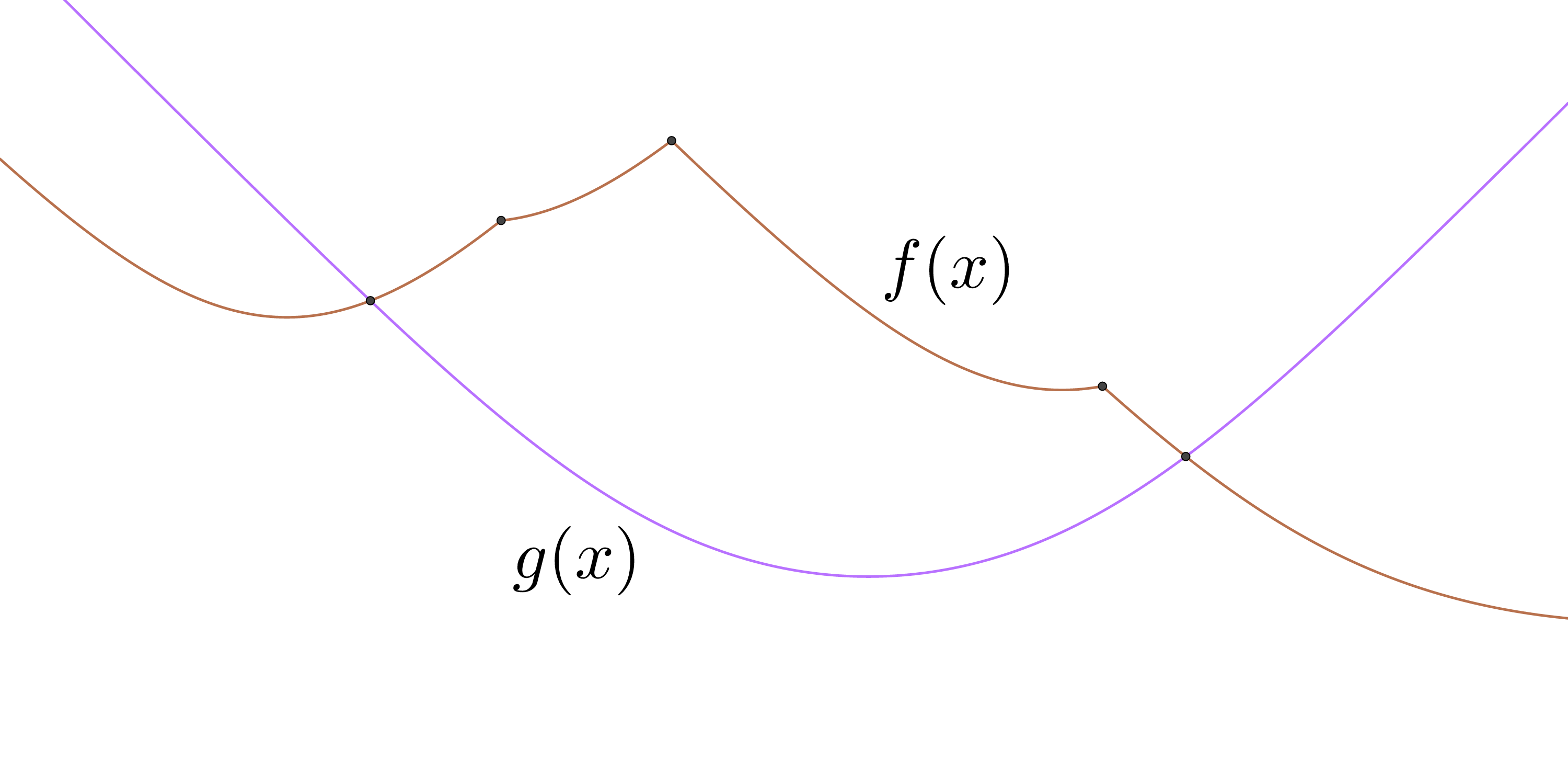
Definition 3.2.4.
By we denote the set of twice continuously differentiable functions satisfying . A continuous function is -concave if for each we have , where , and (see Figure 3).
A continuous function is -concave if it becomes -concave when restricted to every unit speed geodesic.
An element of is a linear combination of and and is defined uniquely by values at two points.
The last tool we need is:
Lemma 3.2.5.
Let be a Fuchsian manifold with convex boundary. Then the function is -concave.
Proof.
Let be a function. We skip proofs of two elementary facts below, which can be proven in the same way as in the theory of concave functions.
Claim 1.
Assume that for every there exists a neighbourhood of in for which is -concave. Then is -concave over .
Claim 2.
Assume that has the left and the right derivatives at every point. Then is -concave if and only if for every sufficiently close and with (resp. ) we have , where is a unique function such that and is equal to the right (resp. the left) derivative of at .
The proof of the next Claim is also straightforward.
Claim 3.
[1, Lemma 2.1] Let be a line in and be the hyperbolic sine of the distance to . Then the restriction of to every unit speed geodesic is in .
We adapt Liberman’s method [41], [5, Lemma 1 in Chapter IV.6]. Let be a unit speed geodesic and be the union of all segments connecting points of the image of with their orthogonal projections to . By abuse of notation, we denote by . The surface can be developed isometrically to a subset of by straightening its lower boundary curve. We denote its boundary components by and .
The curve is a geodesic segment. The set is convex. Indeed, otherwise there are two arbitrarily close points such that the geodesic segment connecting them lies above . Its length is smaller than the length of between and . On the other hand, this segment corresponds to a curve that lies above in the ambient Fuchsian manifold and connects the preimages and of and under the developing map. Due to Corollary 2.2.2, the length of this curve is at least the length of its orthogonal projection to . Hence, it is at least . We can choose and so that the segment of between and is a shortest path. This is a contradiction.
The number is equal to the distance from to . Let and be the base of the perpendicular from to . Due to convexity of , there exists the right half-tangent to at . This is well-known in the Euclidean case and extends to the hyperbolic case with the help of the Klein model. Parametrize with the unit speed and denote the distance from to by . By denote the angle between and the segment .
Claim 4.
The right derivatives of and exist at zero and both are equal to .
Indeed, define . The convexity of implies
In the Euclidean case this is Lemma 2 from [5, Chapter IV.6]. If we consider the Klein model and put in the origin, then we see that this is true in the hyperbolic case also. By we denote the angle between segments and . With the help of Lemma 2.4.3 we get
For the same computations hold.
Thereby, the functions and have the same right derivatives at 0, and due to Claim 3. Let us now prove that for sufficiently small we have . One can prove similar statement for any sufficiently close points and on . Then it follows from Claim 1 and Claim 2 that is -concave.
Let be a point such that is a shortest path between and . By denote the base of perpendicular from . Suppose that . Define . We have . Indeed, to get we need to rotate the segment away from the line . As and , we get .
Now we suppose that . Extend the segment to the intersection with and denote the intersection point by . We have . Define . Due to convexity, . Consider the point . As the triangle is isosceles, we get . Therefore,
We need to get . As , if is not ultraparallel to , then this is true for any . Otherwise, we assume that is sufficiently small, so lies on the same side with from the closest point of to . Thus, and the proof is finished. ∎
Now we have all the ingredients that we need.
Proof of Lemma 3.2.1..
Let be a flat point. Due to Lemma 3.2.3, belongs to the convex hull of non-flat points. The Caratheodory theorem (normally it is stated for Euclidean convex bodies, but this does not matter because of the Klein model) implies that it belongs to the convex hull of at most four non-flat points. If this number can not be reduced to at most three, then must be an interior point of . Thereby, belongs either to the relative interior of a segment with non-flat endpoints and or to a triangle with non-flat vertices , and that is extrinsically geodesic in . Consider the first case. Parametrize by length. Note that restricted to an extrinsically geodesic segment in is : this is Claim 3 from the previous proof. As coincides with at the endpoints of , by Lemma 3.2.5 we have . In particular . In the second case, let be the edge of opposite to . Similarly, we have . Connect with a point by a geodesic passing through . This is possible as is extrinsically geodesic in , so it is isometric to a hyperbolic triangle. Applying the same arguments to we still get that . In the same way one can show that . Thus, . ∎
We showed that to prove Theorem A it is enough to show that coincides with at all non-flat points.
3.3 Polyhedral approximation
Let be a marked Fuchsian manifold with convex boundary, so is a CBB() metric space. In this subsection we will understand how it can be approximated by convex polyhedral Fuchsian manifolds.
We will consider various convex surfaces in . We mark all of them with the help of the vertical projection map (along the perpendiculars to ). Their intrinsic metrics and height functions are pulled back to with the help of marking maps. In particular, this induces a marking on .
The embedding of the universal cover of as determines a representation of as a Fuchsian subgroup of isometries of : it leaves invariant the plane . The quotient by this action of the closed invariant half-space of containing is called the extended Fuchsian manifold and is denoted by . It is homeomorphic to .
We need also to define several classes of triangulations:
Definition 3.3.1.
A geodesic triangulation of is called short if all triangles are convex, all edges are shortest paths and all angles are strictly smaller than . It is called strictly short if additionally all edges are unique shortest paths between their endpoints.
Definition 3.3.2.
A geodesic triangulation of is called -fine if for every triangle we have and .
Lemma 3.3.3.
For every there exists a strictly short -fine triangulation of . Moreover, each triangulation can be refined to a strictly short -fine triangulation (by adding new vertices).
Proof.
The proof is the same as in CBB(0) case [53, Lemma in Chapter III.1, p. 134]. However, Pogorelov uses the intrinsic curvature instead of . This can be easily fixed as the area of sufficiently small triangles uniformly diminishes. ∎
Consider a sequence of positive numbers and a sequence of finite -dense sets . Take the convex hull of in and obtain a convex Fuchsian manifold with polyhedral boundary. By we denote its boundary metric. Here the convex hull is considered in the totally convex sense: the inclusion-minimal closed totally convex set containing .
Lemma 3.3.4.
The metrics converge uniformly to .
Proof.
We follow the ideas from [23, Lemma 3.7] and [15, Lemma 10.2.7]. Unfortunately, some details are less straightforward in our setting.
Let , be the height functions of , . The sequence converges to in the Hausdorff sense. This implies that converges to uniformly, i.e.,
(note that ).
Claim 1.
Let , be two convex surfaces in an extended Fuchsian manifold , and be their height functions and , be their intrinsic metrics. Assume that and
Then .
The proof easily follows from Corollary 2.2.2 and is the same as in [23, Lemma 2.12], we do not provide it here. Claim 1 and imply with .
Next we claim that for each the function defined by the equation
is the height function of another convex surface in . Indeed, as is convex, its Euclidean height function is concave. Due to (3.1), the Euclidean height function of the surface defined by is different from just by multiplication by . Thus, it is also concave and its graph is a convex surface.
The transformation is an analogue of homothety in our setting.
We can choose a sequence such that and converges uniformly to . Denote by , the respective surface by and let be the intrinsic metric of . From Claim 1 we obtain with .
It remains to relate with . First, we check how the distances in change. Fix , let and be the corresponding points. Define , . We want to show that there exist numbers independent of , such that This follows from
Claim 2.
Let and be two ultraparallel trapezoids with
(here we use the notation from Subsection 2.4 and mark the parameters of the trapezoid with prime symbol). By we denote the distance between lines and . For by we denote the space of such pairs of trapezoids with and . Define the function as Fix and let . Then
First we finish the proof of the Lemma and then give a proof of Claim 2. As is compact, the function is bounded from below and from above by positive constants. Let be the lifts of to the universal cover such that . The line passing through , is ultraparallel to the lower plane . Let be the closest point from this line to . If lies outside the segment , then it lies above and is at least the infimum of . If lies between and , then due to Corollary 2.4.5 we have
As , we get that there exists such that . Thus, we can apply Claim 2 and get with .
Now connect and by a shortest path . Let be its image under the vertical projection. It is rectifiable. Consider a polygonal approximation of with sufficiently small segments. It corresponds to a polygonal approximation of of total length multiplied by at most . As the lengths of and are the suprema of the lengths of their polygonal approximations, we get
In total, we obtain uniformly.
∎
Proof of Claim 2..
The space of all ultraparallel trapezoids up to isometry can be parametrized by , and with , and as follows. First we choose two ultraparallel lines at distance . Let be the closest point on the upper line to the lower line. We choose to the right from such that its distance to the lower line is . Then we choose to the right from if is positive and to the left if is negative. One can see that two trapezoids are isometric if and only if the parameters are the same.
The trapezoid is determined by and , hence for each we can consider as a subset of . The closure is compact (note that ) and is obtained by adding the degenerated trapezoids with . We want to show that the function extends there continuously. Indeed, by Lemma 2.4.4 we get
Applying Lemma 2.4.4 the second time we eliminate the angles:
Now for arbitrary we consider the set
and its closure . The function is a continuous function over this compact and is equal to 1 as . The claim follows. ∎
Corollary 3.3.5.
Proof.
The first statement is trivial. For the second we use Theorem 9 of [6, Chapter 8]. ∎
Let be a geodesic triangle in . By denote the 6-tuple of its side lengths and angles in the metric . We will always consider these 6-tuples as points of endowed with metric.
Lemma 3.3.6.
Let be a strictly short triangulation of . Consider a sequence of finite -dense sets with such that all of them contain and none of them contains a point in the interior of an edge of . By denote the pull back of the upper boundary metric of the convex hull of in defined as above.
Then is realized by infinitely many . Moreover, the realizations can be chosen so that they are short and for every triangle we have (after taking a subsequence)
(1) ;
(2) ;
(3)
Proof.
Consider connected by an edge . Connect and by a shortest path in . By we denote the realization of in . By [5, Chapter II.1, Theorems 4 and 5] applied to the intrinsic metric space , for every the sequence converges uniformly (up to taking a subsequence) in as parametrised curves to a rectifiable path of length at most . As is the unique shortest path in between its endpoints, we have .
Choose such that -neighborhoods of vertices of in do not intersect. Then we choose such that for every pair of edges and , -neighborhoods of intersect only if and share an endpoint and if they do, then the intersection lies in the -neighborhood of . For sufficiently large , belongs to -neighborhood of . This means that and can intersect only if and share an endpoint. But in this case they can not intersect except at this endpoint by the non-overlapping property: if two shortest paths have two points in common, then either these are their endpoints or they have a segment in common, see [5, Chapter II.3, Theorem 1].
It is clear now that the union of gives a realization of in . We will continue to work with this realization. The convergence of side lengths of each triangle is already shown. Now we proceed to diameters and areas.
Let be the vertical projection map. We claim that converge uniformly to in the metric . To see this, first project everything to . Denote the images by and . The curves converge uniformly to in and the projection to contract -distances. Therefore, converge uniformly to in . It remains to recall that is the graph of a Lipschitz function , hence for some constant , where is the intrinsic metric of .
The convergence of the diameters follows easily from this and the uniform convergence of the metrics. For the convergence of areas we apply Theorem 8 of [6, Chapter 8].
Let us prove now the convergence of angles. Consider and let be the sectors between the edges of emanating from in the cyclic order. We claim that a proof of the bound
follows line by line the proof in the Euclidean case, see [5, Chapter IV.4, Theorem 2].
Assume that for and some we have
Then for some we have . This contradicts to
Claim 1.
For each and each we have
∎
Proof of Claim 1..
Consider the universal covers , of and . We use the Klein model of embedded into as the interior of the unit Euclidean ball . By and denote the Euclidean and the hyperbolic metrics on respectively. We assume that is developed to the origin. Both and are also convex surfaces in the Euclidean metric. By we denote the intrinsic metric on induced by . We want to show that
Let be the Euclidean ball with the radius and center . Comparing the Euclidean and the hyperbolic metric one can see that the identity map between and is bi-Lipschitz with constant such that as , where and are the Euclidean and the hyperbolic metrics respectively on .
Let and be two geodesics on in the metric emanating from . Due to the bi-Lipschitz equivalence of small neighborhoods of it is easy to see that the angle is also defined and is equal to . Let , be two points, connect them by shortest paths , with in the metric . By definition, . Using the definition of the total angle as the supremum of sums of angles between consecutive geodesics, we get . The converse inequality could be obtained in the same way.
Consider the tangent cone to at in the Euclidean metric (see [5, Chapter IV.5]). Its total angle is equal to [5, Chapter IV.6, Theorem 3]. Similarly there exists the tangent cone to at with the total angle The latter tangent cone is inscribed in the former. We note that for the Euclidean convex cones minus the total angle is equal to the area of the Gaussian image. This shows the desired inequality. ∎
3.4 Statements of the stability lemmas
Our proof of Theorem A is based on several lemmas, but even their statements are slightly cumbersome. Hence, we are going to discuss each one before we formulate it.
From Lemma 2.6.3 we know that if is a convex polyhedral Fuchsian manifold (so it does not have cone-singularities) and is another convex (polyhedral) Fuchsian cone-manifold with isometric upper boundary, then . We need to find a better quantitative lower bound on . Naturally, such bound should depend on and on global geometry of . To our purposes it is enough to treat only the case when there exists such that .
A difficulty arises on our way: the bound we obtain depends on the curvature of a point with . This implies additional complications in our proof of Theorem A. Imagine that for two Fuchsian manifolds with isometric convex boundaries we have in a point with zero curvature. Then when we approximate these manifolds by polyhedral ones, the curvature of in the approximation goes to zero and we are unable to use our quantitative result. Luckily, from results of Subsection 3.2 we can choose to be non-flat. However, this does not mean that the curvature of stays bounded from zero in the approximations: imagine the case of smooth boundaries. But it guarantees that the curvature of a small neighbourhood of this point actually stays bounded from zero. This means that we should be able to handle the case when we have a lower bound on the curvature of a set of points where is distinct from , but not at any precise point. This leads us to the following technical statement:
Lemma 3.4.1 (Main Lemma I).
Let be a convex cone-metric on , , be a convex polyhedral Fuchsian manifold and be a convex (polyhedral) Fuchsian cone-manifold. Let be a subset of vertices. Define
Assume that for all we have , thereby, . Then
Note that if , then and the statement is easier to perceive. At the first reading we advice the reader to consider this case.
We conjecture that the presence of in our Main Lemma I is excessive and it should be possible to give a bound without it. This would have simplified our exposition and also is helpful for a resolution of the Cohn-Vossen problem for Fuchsian manifolds.
Remark 3.4.2.
The function is positive and is increasing in , , and in the range , and . The definition of implies that .
Now we discuss Main Lemma II. A natural way to approximate a metric by cone-metrics (not relying on a convex isometric embedding) is to take a sufficiently fine geodesic triangulation and to replace each triangle by a triangle from a model space (e.g., ) with the same side lengths. However, it turns out to be insufficient for our purposes. We propose a new way to approximate CBB metrics: we replace each triangle of by a triangle with the same side lengths, the same angles and one conical point in the interior. This is the subject of Main Lemma II. A big advantage is that the curvature of each vertex and each triangle of coincides in both approximating and approximated metrics. We hope that Main Lemma II with its proof are of independent interest.
Recall from Subsection 3.3 that means the 6-tuple of side lengths and angles of a triangle in metric . We consider these 6-tuples as elements of endowed with -norm. We also recall definitions of strictly short (Definition 3.3.1) and -fine (Definition 3.3.2) triangulations.
Definition 3.4.3.
Let be a cone-metric on and be a triangulation of . We call swept with respect to if realizes and each triangle of in has at most one conical point in the interior.
Definition 3.4.4.
Let be a CBB() metric space and be its geodesic triangulation. A convex cone-metric on is called a sweep-in of with respect to if
(1) is swept with respect to ;
(2) for each triangle of we have .
Lemma 3.4.5 (Main Lemma II).
There exists an absolute constant such that if is a convex cone-metric on and is its -fine triangulation into convex triangles, or is a CBB() metric and , in addition, is strictly short, then there exists a unique sweep-in of with respect to .
Next we turn to Main Lemma III, which appears to be decomposed into three parts. It is the core of our proof strategy. Assume that we have two cone-metrics and that are very close in some way and there is a convex polyhedral Fuchsian manifold . We claim that there is a convex Fuchsian cone-manifold such that at some “essential” points and is not significantly smaller than . The idea behind this is that we can transform to with the help of some elementary operations and modify along this transformation so that (1) we control the change of heights of some points; (2) we control the decrement of .
Our transformation of to goes roughly: (1) do a sweep-in of ; (2) transform the metric in “the class” of sweep-ins; (3) restore from its sweep-in. The transformation of cone-manifolds corresponding to the first part is Main Lemma IIIA, to the second part is Main Lemma IIIC, to the third part is Main Lemma IIIB.
Lemma 3.4.6 (Main Lemma IIIA).
There exists an absolute constant with the following properties. Let be a convex cone-metric on , be a short -fine triangulation of , be a sweep-in of with respect to and be a convex Fuchsian cone-manifold. There exists such that
(1) for each ;
(2)
Lemma 3.4.7 (Main Lemma IIIB).
For any numbers there exists with the following properties. Let be a convex cone-metric on with
be a -fine triangulation of , be a sweep-in of with respect to and be a convex Fuchsian cone-manifold. Then there exists such that
(1) for each ;
(2)
Lemma 3.4.8 (Main Lemma IIIC).
Let be a convex cone-metric on swept with respect to a triangulation . For each there exists with the following properties. Let and be convex cone-metrics on swept with respect to and for each triangle of we have
Let be a convex Fuchsian cone-manifold. Then there exists such that
(1) for each ;
(2)
3.5 Proof of Theorem A
Suppose the contrary. We identify the upper boundaries of and with the help of and further identify them with for a CBB() metric (see the end of Subsection 3.1). Let and be the corresponding height functions. Because the heights of non-flat points together with the upper boundary metric determine uniquely a Fuchsian manifold with convex boundary (Lemma 3.1.1 and Lemma 3.2.1), there exists a non-flat point such that . Without loss of generality assume that . Define
Let be an (open) geodesic triangle with containing in the interior. Define
Take as the minimum of from Main Lemma II, IIIA and from IIIB for these . Construct a strictly short -fine geodesic triangulation of with the help of Lemma 3.3.3. We can assume that
(1) ,
(2) subdivides in the sense that there is a subset of triangles of such that , where , are the closures of , .
Indeed, if this is not the case, we can refine to a triangulation for which this is true. It might happen that the new triangulation is not strictly short. But due to Lemma 3.3.3, we can refine it further, finally obtaining a triangulation fulfilling all our demands, which we continue to denote by .
By denote the set of those vertices of triangles from that belong to (recall that is open). So we have .
Due to Main Lemma II, there exists a sweep-in of with respect to . Let be from Main Lemma IIIC for , and .
We have two convex Fuchsian manifolds with boundary and . Choose a sufficiently dense set containing . Define and to be convex polyhedral Fuchsian manifolds obtained by taking the convex hull of in and respectively. Here and are induced metrics on the boundaries pulled back to with the help of the vertical projections, and, abusing the notation, we denote restrictions of , to , still by and .
Because is non-flat in , we have .
Due to the convergence of inscribed polyhedral manifolds (Lemma 3.3.6 and Corollary 3.3.5) we can choose such that
(1) both and realize ;
(2)
(3) is -fine on , ;
and for each triangle of we have
(4)
Because we can rewrite (4) as
(4)
Denote . As all the angles and the areas of the triangles of in can be chosen to be arbitrarily close to those in , we can assume also that
Let , be sweep-ins of , with respect to . They exist due to Main Lemma II as , are -fine.
First we apply Main Lemma IIIA to and . We get such that
(1) ;
(2)
Now we apply Main Lemma IIIC to and . We get such that
(1) ;
(2)
Finally, we take , and apply Main Lemma IIIB. We get such that
(1) ;
(2)
Summarizing all last three steps together we see:
(1) ;
(2) .
We get .
Now we do the same but starting from and transforming to to to . We obtain such that (here we need only properties (2))
In total, we summarize our main transformations in the following diagram:
Now let
and is defined above. Then Main Lemma I implies that
Recall that we chose such that . Thus, for each we have . We know , due to Corollary 2.2.2. Thus, for each we have , . From this we conclude the bounds on heights with the help of Lemma 2.5.6: for every we obtain
From this we deduce that that , and . Recall also that . Thus, due to Remark 3.4.2 we get
By Lemma 2.6.3 we have
Summing this up we have
Thus, and we obtain a contradiction.
4 Properties of Fuchsian cone-manifolds
In this section we examine some important properties of Fuchsian cone-manifolds.
4.1 Ultraparallelism
Lemma 4.1.1.
Let be a convex Fuchsian cone-manifold. Then each prism of is ultraparallel.
Proof.
Suppose the contrary. Then we construct an infinite sequence of pairwise distinct prisms of .
Suppose that there is a prism of developed to as such that its upper boundary plane intersects the lower boundary plane in line under dihedral angle .
We call the distance function to over the triangle the weight function and its minimum the weight . It is easy to see that the point , where is attained, is unique and belongs to the boundary of . We have
Suppose that is an interior point of an edge (say, ). Then the line is ultraparallel to . We observe that that the dihedral angle of at is greater than . Take next the prism adjacent to at the edge corresponding to . Embed it to adjacent to . Then its upper boundary plane also intersects the lower boundary plane in line . Let be the respective dihedral angle. Due to the convexity condition, the angle of at is smaller than and . To see this one considers the orthogonal plane section to lines and , which exists as they are ultraparallel. We get , where is the weight function of defined as the distance to , and if and only if .
If the weight of is attained at , then its dihedral angle at the edge containing is also greater than . This can not happen as the total angle is at most . Therefore, it can not be attained at and , where is the minimum of .
Now suppose that is attained at a vertex of (say, ). We claim that among the edges incident to there exists at least one with the dihedral angle greater than . Indeed, either the line containing one edge does not intersect and lies from the different side of this line than , then this edge is the desired. Or there is an edge such that lies in the non-obtuse angle formed by and the line containing this edge. Let this edge be .
Now take the prism adjacent to the edge corresponding to and embed to adjacent to . Similarly to the case before, convexity implies that the upper plane of intersects in line with the dihedral angle satisfying . If , then and, therefore, . Suppose that , then is also attained at and , so the upper plane of coincides with .
By denote the line in through orthogonal to oriented outwards to . Assume that lies to the left of and be the angle between and . The condition that is attained at implies that .
Let be the edge of incident to . As , then also lies to the left of and for its angle with we have .
In this way we construct an infinite sequence of prisms of . Two prisms in this sequence are distinguished either by their weight, which decreases monotonously, or, if the weights are equal, by the angle , which strictly decreases as long as the weight remains constant. Clearly, both and are independent of the embedding. This shows a contradiction.
Now it remains to consider the case when the initial prism is asymptotically parallel, i.e., the upper boundary plane intersects the lower boundary plane only at infinity. Let be a horocycle in through the intersection point. We can similarly define the weight function as the distance to . All arguments above remain valid. Moreover, either we will find in our sequence a prism such that its upper boundary plane intersects the lower boundary plane in a line, and then we are reduced to the case above, or all prisms in the sequence after development will have as their boundary plane. ∎
Let be convex and be the extended height function. Take and embed the prism containing to . Lemma 4.1.1 say that this prism is ultraparallel. Let and be the closest points on the upper and lower boundary planes respectively. Due to Corollary 2.4.5, satisfies for every
| (4.1) |
In particular, its restriction to a geodesic segment in has the form
| (4.2) |
We highlight that and may lie outside of the image of in . However, neither nor the distance depend on the choice of representation or embedding.
4.2 Heights define a convex cone-manifold
Consider a convex Fuchsian cone-manifold and a unit speed geodesic . Let be its intersection points with strict edges of . We set and . Due to (4.2), on each segment the restriction of has the form
for some positive . Moreover, the convexity implies that for each kink point we have the left derivative greater than the right derivative (see on Figure 3).
Lemma 4.2.1.
The function is -concave.
Proof.
Let be in and be a function such that
(1) , ;
(2) there is a subdivision
( and ) such that the restriction of to each is ;
(3) at every point the left derivative of is greater than the right derivative.
We claim that for all . Due to the discussion above, this will imply that is -concave.
Claim 1.
Two distinct -functions on can not coincide at more than one point.
This follows from the definition of the -class.
Claim 2.
Let be the extension to of the restriction . For all we have .
Indeed, consider and prove by induction over that for we have . The base case follows from Claim 1 and the fact that in the kink point the derivative of is greater or equal than the derivative of . The inductive step is obvious. The case is the same.
Claim 3.
For all we have .
Indeed, Claim 1 and the assumption imply that the sign of the difference is constant on . Assume that it is negative, i.e., for every we have . Also assume . Substituting and using Claim 2 we obtain that , which contradicts the statement.
Now we may assume that the sign of the difference is positive on : if it is zero, then we just cut off and proceed in the same way. Under this assumption, suppose that for some and , , we have . Due to Claim 1 and the assumption, we have for all . Thus, due to Claim 2 we have for all . We obtain a contradiction.
It implies that over the interval . ∎
We note a simple property of -concave functions similar to a property of ordinary concave functions. Let be a -concave function and coincides with at points . Then for all we get . If for some we have , then for all and for all we get .
Now we are going to prove that a convex Fuchsian cone-manifold is uniquely determined by and . If we know and , then it remains only to restore its face decomposition.
Lemma 2.6.1.
Let and be two triangulations with
and be two convex Fuchsian cone-manifolds. Then is marked isometric to with respect to .
Proof.
Take the intersection point of two edges and . The restriction of to is . Due to Lemma 4.2.1, the restriction of to is -concave. As they coincide at the endpoints of , we get . Applying the same reasoning to , we get . Hence, .
Let be together with all the intersection points between the edges of and . We obtained . The union of geodesic triangulations and decomposes the metric space into geodesic polygons with vertices in . Let be a geodesic triangulation refining this decomposition. The convex Fuchsian cone-manifold is marked isometric to both , due to Corollary 2.4.6. This finishes the proof. ∎
4.3 The space of admissible heights
Recall from Subsection 2.6 that is the set of all admissible heights for the pair , i.e., it is a set of convex Fuchsian cone-manifolds for fixed and . In this subsection we collect key facts about that will be used in the proofs of the main lemmas.
Lemma 4.3.1.
Let and . Define by for all . Then for all , and all Fuchsian cone-manifolds have the same face decomposition.
Proof.
Consider two adjacent prisms such that the dihedral angle of the adjacent upper edge is . Develop them to in the half-space model, let be the plane containing the lower boundaries and — upper. By and denote the closest points. Assume that the line intersects the ideal boundary at point and is between and . The homothety with center is a hyperbolic isometry. Consider the images of all upper vertices of the prisms and their projections to . We obtain two new prisms with upper boundaries isometric to those of former prisms and the dihedral angle of the common upper edge remains equal to .
Assume that Let be the distance function of the new vertices. Due to formula (4.1), for each vertex of the prisms.
Let be a triangulation compatible with , so . We saw that all flat edges remain flat in all . But for sufficiently small all strict edges remain to be strict. Thus if is sufficiently small, then is convex and . However, if a strict edge becomes flat, then it is flat in all . Thus, for all and all have the same face decomposition. ∎
Lemma 4.3.2.
For each and there are finitely many with for which there is such that is compatible with .
Proof.
Due to Lemma 4.3.1, it is enough to prove that there are finitely many compatible with convex cone-manifolds with for some and all .
Let be an edge of . Develop the trapezoid containing as . Let and be the closest points on the lines containing its upper and lower boundaries. Assume that lies between and . Denote the distance by , by and by . Then from Corollary 2.4.5 we get
Then we have
Due to Lemma 2.5.6, we have . Then we get
If lies between and , then one of , is at least . Assume that this is . Note that . Considering the trapezoid , we get similarly
Hence there exists a constant such that the lengths of edges of are at most . But the lengths of geodesics between points of in form a discrete set by an argument from [33, Proposition 1]. Thus there are finitely many of them that can appear as edges of some . Therefore, there are finitely many realizable triangulations. ∎
Define
Lemma 4.3.3.
For every and the set is compact.
Proof.
From Lemma 4.3.2 there are finitely many triangulations compatible with for . For every triangulation the set of heights bounded between and , such that is a representable triple, is compact. Its subset of admissible heights , such that is compatible with the convex cone-manifold , is defined by considering also inequalities for all edges of . Thus, it is a closed subset, hence, also compact. Finally, is compact as a finite union of compact sets. ∎
Now we are going to establish two fundamental properties used in several parts of our proof: even if is on the boundary of , the height of a point with non-positive particle curvature can always be decreased (Corollary 4.3.7) and the heights of all points with positive particle curvatures can always be simultaneously increased (Lemma 4.3.9). Together with this we show how non-positive/positive particle curvature impacts on the upper boundary geometry.
Lemma 4.3.4.
Let be a convex Fuchsian cone-manifold, and either or and . Then all angles at of faces incident to are strictly less than .
Proof.
Lemma 4.3.5.
Let and be two adjacent compact prisms in such that the total dihedral angle of the common edge is . By denote the total angle of in the upper faces. Then
Proof.
We highlight that is the face angle opposite to ! For the angle at in the trapezoid from Lemma 2.4.3 we have
Consider the spherical link of in the union of both prisms. It consists of two spherical triangles glued altogether. When changes, only the common edge changes and the derivative is positive. Let , be the dihedral angles of in two prisms and , be the angles at of their upper boundaries. Then
So we get
This implies the desired. ∎
Lemma 4.3.6.
Let be a convex Fuchsian cone-manifold and be a vertex that has angle less than in all faces. For define by and for all , . Then provided is sufficiently small.
Proof.
The proof ideas are essentially due to Volkov [69]. It was also reproduced for cusps with particles in [21]. We sketch it here because the ideas from the proof are used further.
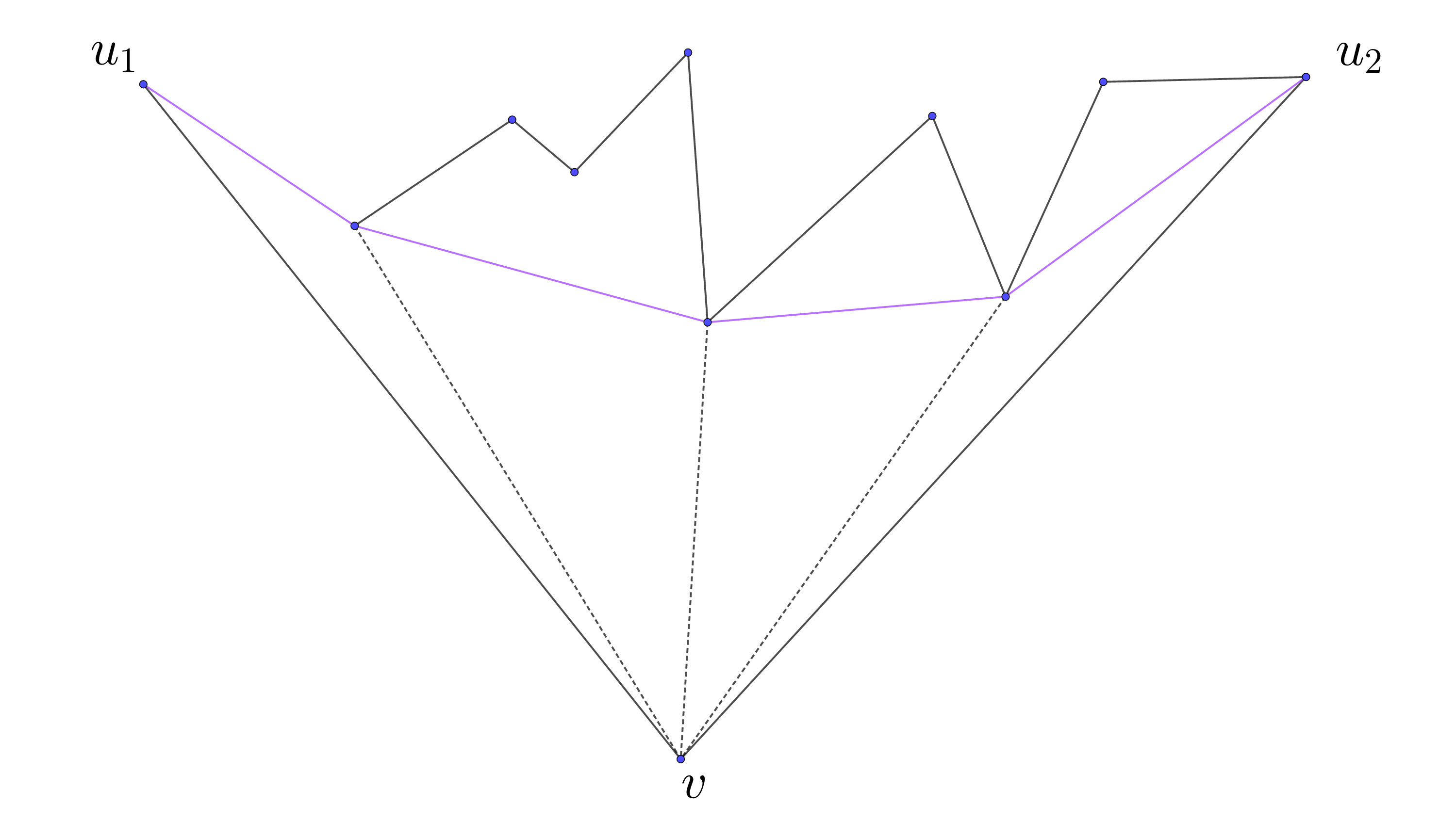
Let be a vertex such that it has angle less than in all faces of . We claim that each face can be triangulated such that all new flat edges become convex after we decrease the height of . Let be a face incident to and , be two vertices incident to . Consider the shortest path in connecting and and homotopic to the polygonal curve (see Figure 4). This path is a polygonal curve that cuts off a polygon such that it has angles greater than at all vertices except , , . Triangulate it by diagonals from . Lemma 4.3.5 shows that this triangulation is a desired one. ∎
Corollary 4.3.7.
Let be a convex Fuchsian cone-manifold and be a vertex with either or and . For define by and for all , . Then provided is sufficiently small.
Recall that a vertex of is called isolated if there are no strict edges emanating from it.
Lemma 4.3.8.
If is an isolated vertex of a Fuchsian cone-manifold , then
Proof.
Consider a triangulation compatible with and start developing all prisms containing to one by one preserving the incidence, each prism developed only once. We get a chain of prisms with all lower boundaries belonging to the same plane and all upper boundaries belonging to the same plane as all upper edges are flat. It is easy to see that as , then with the equality in one case implying the equality in the second case. Thereby, our chain of prisms is not self-intersecting. Assume that . The first and the last upper edge of the development are images of the same edge of , therefore the distance function restricted to these edges is the same. Due to condition that the sum of the dihedral angles at this edge is , we see that is developed to the closest point from to . This gives the desired equality. ∎
Lemma 4.3.9.
Let be a convex Fuchsian cone-manifold and . For define by if and otherwise. Then provided is sufficiently small.
Proof.
Lemma 4.3.2 shows that there are finitely many triangulations compatible with . Consider sufficiently small such that for any compatible with all strict edges of remain strict in . We start from an arbitrary triangulation and use the flip algorithm to find a triangulation such that is convex. The flip algorithm will also be used in some further parts of the proof.
We simply take a concave edge of and flip it, i.e., replace by the other diagonal in the quadrangle formed by two triangles incident to . There are two questions: why the algorithm can not run infinitely and why a concave edge can be flipped.
By induction it is easy to see that each triangulation that appears is compatible with . Indeed, if this is true for the current triangulation, then by the choice of all strict edges of are strict in . Therefore, they can not be flipped and the new triangulation is also compatible with . The extended height function is pointwise non-decreasing after each flip. Moreover, it strictly increases at all the interior points of the quadrangle defining the flip. This means that no triangulation appears twice during the algorithm. As there are finitely many of them, the algorithm can not run infinitely.
There are two cases, when an edge can not be flipped. First, it can be an edge of a triangle with two sides glued altogether, so there is no quadrangle at all. Second, it can be a diagonal in a concave quadrangle. We illustrate this by Figure 5.
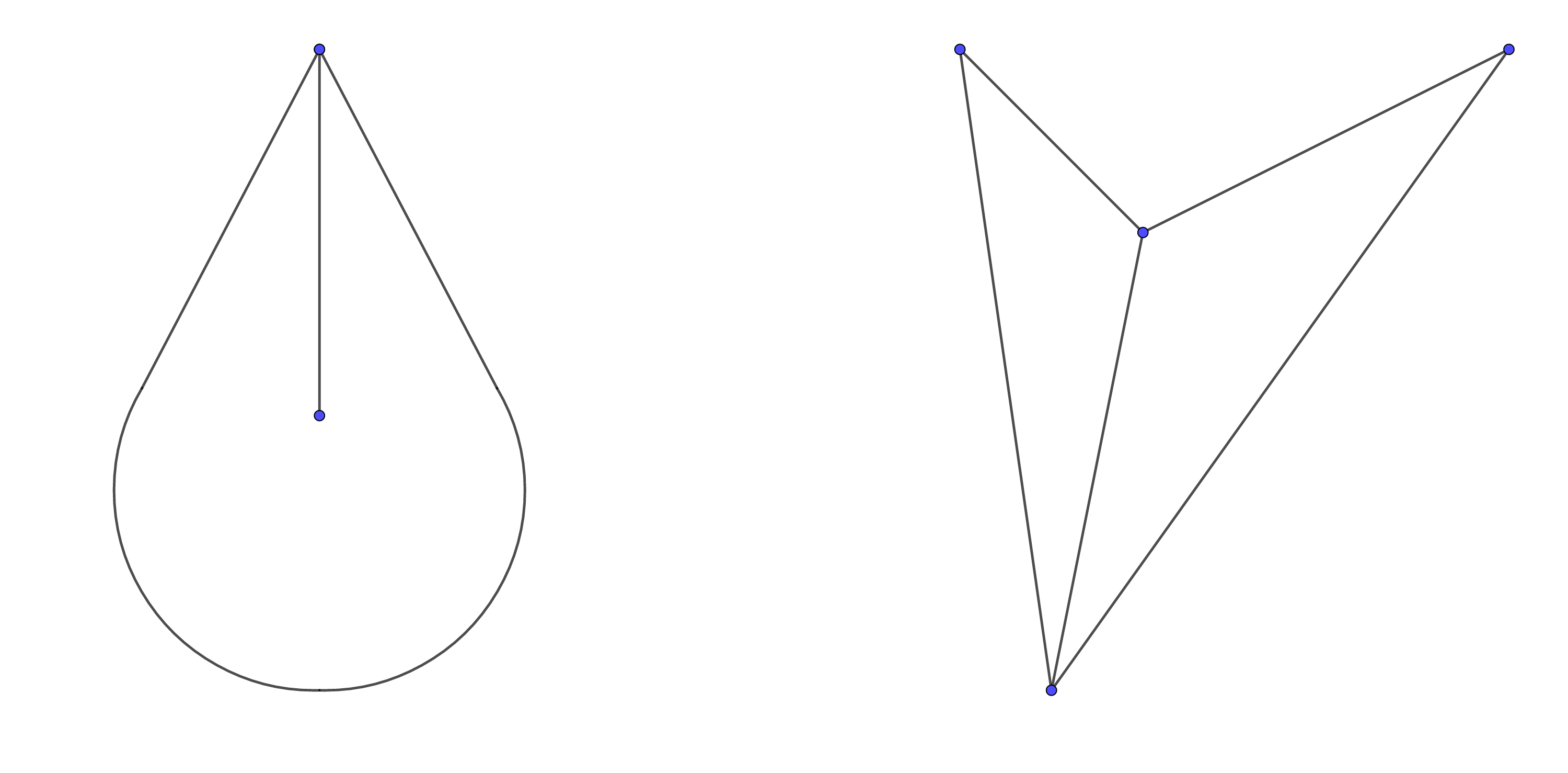
We prove that under our conditions this can not happen. Suppose that for some an edge is incident only to one triangle , is the vertex incident only to and is the other vertex of . Then . The edge is flat in , thus, is isolated in . Lemma 4.3.8 implies that , so . If also , then remains flat in (see the proof of Lemma 4.3.1). Consider the case . Note that as is isosceles, then both angles of at are smaller than . Therefore, becomes convex in due to Lemma 4.3.5.
Suppose that for some an edge is a diagonal of a concave quadrilateral and is the vertex of this quadrilateral with total angle at least . The edge is flat in . Lemma 4.3.4 shows that (as , we have ) and, therefore, . If this is true for all vertices of the quadrilateral, then remains flat in . We prove that in all other cases becomes convex.
Indeed, denote three other vertices by , , such that connects and . If only increased its height, then the claim follows from Lemma 4.3.5. Otherwise, we first increase the heights of all , , by . The edge stays flat. If we decrease now the height of , then becomes convex due to Lemma 4.3.5. If we decrease the heights of or , then it is clear that the dihedral angle of decreases. This also applies if we need to decrease heights of several of them. Thus, all cases are considered. ∎
Lemma 4.3.10.
Let be a convex Fuchsian cone-manifold such that all faces are strictly convex hyperbolic polygons. Then is in the interior of .
Proof.
The proof is similar to [21, Proposition 3.15(2)]. Lemma 4.3.2 shows that there are finitely many triangulations compatible with . We can choose a small enough neighbourhood of in such that for any such triangulation and any all strict edges of remain strict in . Then the flip algorithm from the proof of Lemma 4.3.9 performs inside each face of separately. Therefore, it finds in finitely many steps a triangulation such that is convex. ∎
Lemma 4.3.11.
If a face contains a curve, which is not homotopic to a point in , then it contains a face angle greater than .
Proof.
We cut along geodesic segments until it becomes simply connected (the existence of such set of cuts follows, e.g., from Lemma 2.3.6). Before the last cut we have an annulus . Let and be two its boundary components, be the geodesic segment between them that defines the last cut and be the resulting polygon. Each cut only decreases the values of the angles, hence it is enough to prove that there is an angle at least before the last cut.
If there are no angles greater than in , then is convex. Develop the prisms having upper boundaries in to . Note that as is convex, the development is not self-intersecting. Let , be geodesic segments, which are images of , be the plane containing the lower boundaries and — upper. Denote by and their closest points. The distance function from and to coincides at the respective points. Therefore, the trapezoids containing and are isometric. There exists a unique orientation-preserving isometry of mapping one trapezoid to the other. Because is orthogonal to both trapezoids planes, it is preserved by this isometry. Because corresponds to a flat edge of , also must be preserved by this isometry. This means that this is a rotation along the line at the angle smaller than , which maps to . Because is a convex polygon, when we consider the restriction of this rotation to , we get an embedding of to a convex hyperbolic cone. Assume that is embedded closer to the apex than . Write the formula for the area of the cone-polygon bounded by in terms of the angles. We see that contains in an angle greater than . ∎
Corollary 4.3.12.
Let be a convex Fuchsian cone-manifold with such that for all we have . Then the graph of the strict edges of is connected and all faces are strictly convex hyperbolic polygons. In particular, .
Remark 4.3.13.
A crucial difficulty for some of our arguments is given in the fact that is not convex for a cone-metric . However, it becomes convex if we do the coordinate change . But in these coordinates the discrete curvature functional does not have the magical properties that we need.
4.4 First variation formulas
Let be a convex Fuchsian cone-manifold. Recall from Subsection 2.6 that its discrete curvature is
(This makes sense not only for convex Fuchsian cone-manifolds, but we are interested only in convex ones.) Clearly, is independent from the choice of compatible with and is a continuous functional on in the coordinates .
Fix . For a subset define
This set is endowed with the topology induced from the product topology. Any point of can be considered as a convex Fuchsian cone-manifold with the vertex set . We can define over . In order to understand its behaviour we need to introduce charts on related to geodesic triangulations of .
First, for a triangulation with the vertex set denote by the set of all admissible such that is compatible with . This defines a subdivision of into subsets corresponding to different triangulations. It is evident that the boundary of is piecewise analytic.
Next, define the set as the set of pairs , where , . The boundary of the set is piecewise analytic. In the chart on the functional is a continuous function of heights and lengths of the upper edges .
Lemma 4.4.1.
is continuously differentiable over and
Remark 4.4.2.
The set has boundary. By continuously differentiable at the boundary points we mean that all partial derivatives admit a continuous extension there.
Remark 4.4.3.
The partial derivatives are not defined for flat edges of cone-manifolds corresponding to boundary points of . For these points they make sense only as directional derivatives along paths for which these edges become strict.
Proof.
The set is locally modelled in , where and is the number of edges of any triangulation of with vertices.
Assume first that belongs to the interior of some . Then the combinatorics of Fuchsian cone-manifolds in a neighbourhood of does not change and all the dihedral angles can be written as sums of dihedral angles in the same prisms. For a single prism each dihedral angle is a smooth function of its lengths and by the Schläffli formula we get
Summing this for all prisms we obtain
Therefore,
This shows the first derivative formula. As the angles are smooth functions of the lengths, we see that is smooth in this case.
Now assume that is not in the interior of any . This means that either some vertices of have the total angle or there are flat edges in . In any case, all boundary conditions are piecewise analytic. Let be the set of strict edges of . By we denote any triangulation with vertices at realized by containing all edges from , so it is compatible with . (By Lemma 2.3.6 such a triangulation exists.) It provides a chart over in . Now let be the point corresponding to and be a vector such that for all sufficiently small . Then, as all boundary conditions are piecewise analytic and the number of triangulations compatible with is finite, there exists such that for all sufficiently small . The triangulation might be different from , but it contains all edges from .
From the previous argument, we get
where , are the corresponding coordinates of . The second sum is only over strict edges as flat edges give zero directional derivatives at . Thus, all partial derivatives exist and are continuous in a neighbourhood of . We see that is continu ously differentiable and its first derivatives are the respective curvatures. ∎
4.5 Second variation formulas
Now we are going to investigate the second derivatives of over (we do not consider the second derivatives with respect to the upper boundary). To this purpose we need a new notation.
By we denote the set of oriented edges of in the sense that each edge gives rise to two oriented edges with respect to two different possible orientations. By we denote the set of oriented edges starting at and by we denote the set of oriented edges starting at and ending in . In particular, is the set of loops from to itself and each loop is counted twice. For compatible with and by and we denote the dihedral angles of in the right and the left prisms incident to respectively. By we denote the angle of the trapezoid containing at the vertex, where starts. By and we continue to denote the lengths of in the upper and the lower boundaries of respectively.
Lemma 4.5.1.
Let . Then is twice continuously differentiable over and
Proof.
Similarly to the proof of Lemma 4.4.1, it is enough to prove the claim for in the interior of a set of heights such that is compatible with the respective cone-manifold. This is reduced to computations for a single prism .
Consider a spherical link at the vertex . From the cosine rule we get
Differentiating the spherical cosine rule, we obtain
Differentiating the cosine rule for trapezoids from Lemma 2.4.3, we see
So we have
| (4.3) |
| (4.4) |
Lemma 4.5.2.
Fix and identify with a subset of . The Hessian of over is non-positive definite. Moreover, its kernel is spanned by vectors defined by if and 0 otherwise, where is an isolated vertex of .
Proof.
We have
From Lemma 4.5.1 we see
Hence, the Hessian is non-positive definite. Also if and only if there are no strict edges in between and . Thus, it is easy to see that if and only if has non-zero coordinates only on isolated vertices of . ∎
Thus, is concave over .
Remark 4.5.3.
Although the Hessian of can be degenerate and, moreover, critical points might be non-isolated, one can show that it can not be degenerate along any segment in . Thus, is strictly concave over . In what follows we will not need it, so we do not prove this. This would lead to a proof of local rigidity of convex Fuchsian cone-manifolds.
Together with Lemma 4.3.8 we get
Corollary 4.5.4.
Let be a convex Fuchsian cone-manifold with such that for all . Then is non-degenerate at .
4.6 Behaviour of at infinity
The set is non-compact and we need to understand the behaviour of outside a compact set. In particular, we will prove the maximization principle Lemma 2.6.3.
Lemma 4.6.1.
Let . For each there exists such that if and for some vertex one has , then we get .
Proof.
Claim 1.
For each there exists such that if the side lengths of a hyperbolic triangle are at most , then the sum of its angles is at least .
This is because the area of a hyperbolic triangle is equal to the sum of its angles minus . By computing the Euler characteristic we get
Claim 2.
For each there exists such that if for a Fuchsian cone-manifold for each the length of the projection of to is at most , then
The number of triangulations compatible with some is finite for fixed , due to Lemma 4.3.2. Due to Lemma 2.4.3, if a trapezoid has fixed upper edge and growing heights, then its lower edge becomes smaller. Thus, we conclude
Claim 3.
For each there exists such that if and for each we have , then for each edge of we have .
From the finiteness of the set of compatible triangulations we also get
Claim 4.
There exists such that for any convex Fuchsian cone-manifold compatible with a triangulation we have
Finally, the triangle inequality for trapezoids (Lemma 2.5.6) gives
Claim 5.
For every there exists such that if and for some we have , then for each we get .
Combining all these claims together we see that for every and we can choose such that if and for some , then we get
As and is arbitrary, this finishes the proof. ∎
Corollary 4.6.2.
For every , and the set is compact.
Now we turn to cone-manifolds with small heights.
Lemma 4.6.3.
If is a sequence such that for some we have , then for all we get and , where are particle curvatures in . Also for every edge of all we have , where is the dihedral angle of in .
Proof.
Lemma 4.3.2 implies that there are finitely many triangulations compatible with some . Hence, up to taking a subsequence we may suppose that the same triangulation is compatible with all .
Take connected with by an edge of . If for some we have , then the trapezoid corresponding to becomes not ultraparallel for large enough . This contradicts Lemma 4.1.1. Hence, . By the connectivity of the edge graph of , this extends to all vertices.
Take an oriented edge emanating from . Develop the trapezoid containing from to as . Let and be the closest points on the lines containing the upper and the lower boundary respectively. We have . Denote by . Clearly, , hence . From Corollary 2.4.5 we get
Hence, . Now we take a triangle of and the prism from containing . Let be incident to , be the angle of at , be the dihedral angle of the respective lateral edge and be the dihedral angle of in the prism. Consider the spherical link of . As all , we obtain and . Thereby, , and . ∎
Thus, when some heights tend to zero, the upper boundary falls down to the lower boundary as we could expect. Lemma 4.6.3 together with Lemma 4.3.2 imply
Corollary 4.6.4.
Let be the origin. The functional with its partial derivatives can be continuously extended to over by putting , .
Now we are ready to prove the maximization principle from Subsection 2.6:
Lemma 2.6.3.
Let , be the convex polyhedral Fuchsian manifold realizing and be a convex Fuchsian cone-manifold distinct from . Then .
Proof.
We want to show that there exists at least one global maximum of over and there are such that all global maxima are contained in , where
Indeed, an upper bound follows from Lemma 4.6.1. If there is no lower bound, then we have a sequence of global maxima converging to . Lemma 4.6.3 implies that all become positive at some point . Lemma 4.3.1 shows that we can increase all heights of , which increases , so was not a maximum point. This means that we can find such that contains all global maxima and at least one global maximum exists.
Let be a convex Fuchsian cone-manifold that is a local maximum (not necessarily strict) of over . We claim that it is actually a convex polyhedral Fuchsian manifold. Indeed, if there is such that , then due to Corollary 4.3.7 we can decrease while staying in . Due to Lemma 4.4.1 this increases . If there is a vertex such that , then Lemma 4.3.9 shows that we can increase simultaneously the heights of all such vertices and stay in . Again, this increases .
5 Stability lemmas
5.1 Proof of Main Lemma I
5.1.1 Dual area
Let be a convex Fuchsian cone-manifold. In Section 2.5 we defined the spherical link of a vertex . Intrinsically it is a disk with a spherical cone-metric that has (at most) one conical point in the interior, piecewise geodesic boundary and the angles of all kink points of the boundary are less than . Geometry of spherical links is highly connected with the behaviour of the discrete curvature. In order to get the quantitative bound of Main Lemma I, first we prove an inequality concerning spherical links, which will be used further in estimating the derivatives of the discrete curvature.
Lemma 5.1.1.
Let be a disk with a spherical cone-metric that has a single conical point in the interior of total angle and of curvature , and has a piecewise geodesic boundary with kink points denoted in the cyclic order. By denote the length , by and denote the angles and respectively. Assume that , , for each we have and the perimeter of is (strictly) less than . Define . Then
| (5.1) |
Proof.
We start with the case , so . Then there is no conical point, but we assume that is an arbitrary marked point in the interior of .
In this case we develop the polygon to the unit sphere so that coincides with the south pole. Then determines a solid convex cone with the apex at the origin. Consider its polar cone. It defines the polar spherical polygon , which belongs to the open hemisphere centered at the north pole . Project it from the center of sphere to the tangent plane at . We get a Euclidean polygon . If all , then is in the interior of both , . If there are some , then is outside from both of them.
Regardless the location of , one can compute that the left-hand side of (5.1) is exactly the area of and the right-hand side is the area of (in particular this will follow from the general discussion below). Hence, (5.1) is true because the central projection to a tangent plane increases areas.
In the general case one can still consider similar polar polygons (which contain cone-singularities) as long as all . Otherwise the polar interpretation breaks down and , can be defined only in a virtual sense described below.
We call a spherical triangle a (spherical) orthoscheme if , the sides and are either both at most or both at least and is equipped with plus or minus sign. If is equal to , then the orthoscheme is called singular. If , then also automatically and we call double-singular. From simple trigonometry we conclude that if is non-singular, then
Define its dual orthoscheme as a spherical triangle with , and . One can conclude
See Figure 6. For a non-singular orthoscheme the sign of is defined as the sign of if or as the converse sign otherwise. For a singular orthoscheme, the dual orthoscheme is degenerate and we assign zero as its sign.
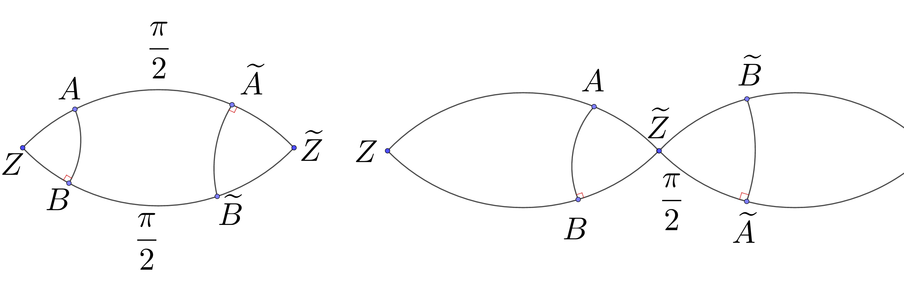
This duality is not involutive. By definition, only orthoschemes with both can be obtained as duals and each such non-degenerate orthoscheme is obtained as the dual of exactly two orthoschemes.
Let be an orthoscheme. Consider the unit sphere and place the dual orthoscheme such that becomes the north pole. Then belongs to the open northern hemisphere. Project it from the center of the sphere to the tangent plane at . The image is called the Euclidean dual orthoscheme to and is denoted by (where ). One can compute the signed areas, i.e., the areas taken with the sign of the dual orthoshemes:
Let be a spherical triangle with both , at least or both at most , but at least one (say, ) not equal to . Put it on the unit sphere and consider the geodesic great circle containing segment . Then there are two perpendiculars from to it. Let be the one such that . The characteristic function of triangle is the signed sum of the characteristic function of triangles , . Consider the latter triangles as orthoschemes endowed with signs coming from this sum. We say that is canonically decomposed into the orthoschemes , . In the case of the canonical decomposition of into orthoschemes is itself taken with the plus sign (then it is a double-singular orthoscheme).
Now we turn to the spherical cone-polygon . Since now we call the kink points vertices of . Cut into triangles . If there are such that and (or the converse), then there exists a unique such that and we add to the set of vertices. Hence, we may assume that for all either both , are at least or both are at most . We decompose each triangle canonically into orthoschemes and call it the canonical decomposition of . By denote the set of orthoschemes of the canonical decomposition. The total angle is the signed sum of angles at in all orthoschemes, similarly is the perimeter . Thereby,
and the inequality (5.1) is equivalent to
Define . We have all , except possibly some with (which correspond to recently added vertices).
Take such that and consider two orthoschemes incident to . Denote them by and respectively. Note that due to convexity at least one of them is positive. Let be the base of perpendicular from to the geodesic in the canonical decomposition. Develop the dual orthoschemes and to the sphere so that they have the segment in common, with opposite orientations if they have the same sign and with the same orientation otherwise (see Figure 7). We say that the triangle obtained this way is the sum of the dual orthoschemes. We equip it with the sign determined from the sum of the characteristic functions of and taken with the respective signs.
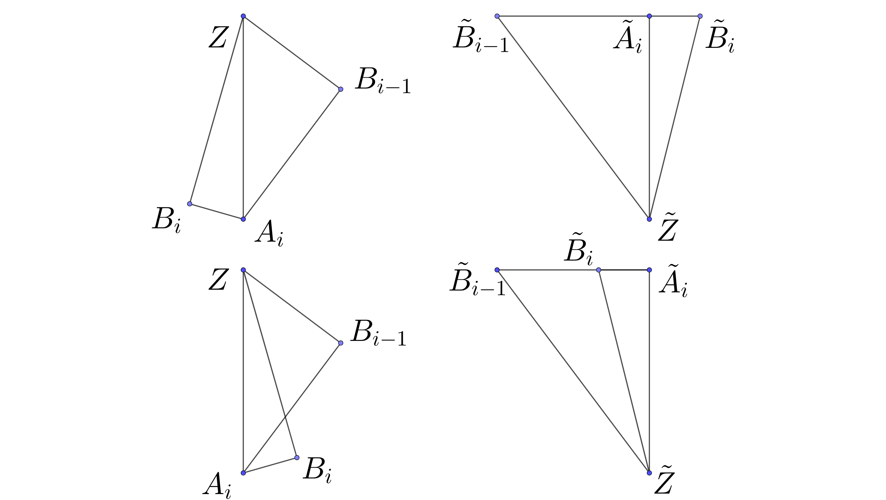
One can see that if , then the sum of the dual orthoschemes is a positive spherical triangle with . We call it a positive pair. We obtain that if , then
because the central projection increases areas.
Similarly, if , then
Therefore, if all , then the proof is finished.
It remains to consider the case, when some , which is much more subtle.
First, we investigate the boundary structure. Let be an oriented circle of length . It naturally parametrizes the set of geodesics emanating from . We say that corresponds to the segment and positive direction corresponds to the order . If is the segment corresponding to , where belongs to the boundary of , then is the angle of the sector between , in the positive direction. Let be the length of . It defines a continuous function on . We now consider the case when for some we have .
Lemma 4.3.4 implies that no geodesic segment in the boundary of has length at least . This clearly means that no geodesic segment in has length at least . Otherwise we can extend this segment until it intersects the boundary and cut off the part of the polygon that does not contain . Then we obtain the cone-polygon with non-positive curvature, small perimeter and geodesic segment in the boundary of length at least , which can not happen.
In particular this means that for each we get . Then there exists such that . We want to show
Claim 1.
There exist exactly two such that .
With the preliminary discussion this means that is subdivided by , into two complementary open intervals such that and .
Indeed, consider such that . Let be the maximal interval containing for which . We saw that . Let be the left and the right endpoints of , so . Let be the vertex of corresponding to . Then . Note that the strict inequality here is because for close to from the left. Consider the interval . Develop the part of corresponding to to the unit sphere. From convexity, and one can see that .
Assume that there are more points such that . Take the closest of them to in positive direction and denote it by . We showed that . Together with this implies that the part of perimeter of between the segments from corresponding to and is greater than . Similarly, we consider that is the closest to in the negative direction such that . We get that the segments corresponding to and also cut off the part of perimeter of length greater than . The intervals and do not intersect. Hence, the perimeter of is greater than , which is a contradiction. Claim 1 is proven.
By we denote the points at the boundary of corresponding to , . Due to our previous agreement, they are vertices even if their angles are . By we denote the sets of vertices corresponding to the segments .
We are going to discuss now what happens with dual orthoschemes. We focus on Euclidean duals, but we note that exactly the same happens with spherical duals. We think that our discussion is easier to imagine on the Euclidean plane.
Take , we get . For two orthoschemes incident to the sum of their Euclidean duals is a negative triangle (recall Figure 7). We call it a negative pair.
Consider all and start developing all dual triangles one by one to the Euclidean plane. The sides constitute a polygonal curve , which we denote by . See Figure 8. Define
The angle as seen from is
where . This means that the polygonal curve is convex as seen from . From this one can show that and is not self-intersecting.
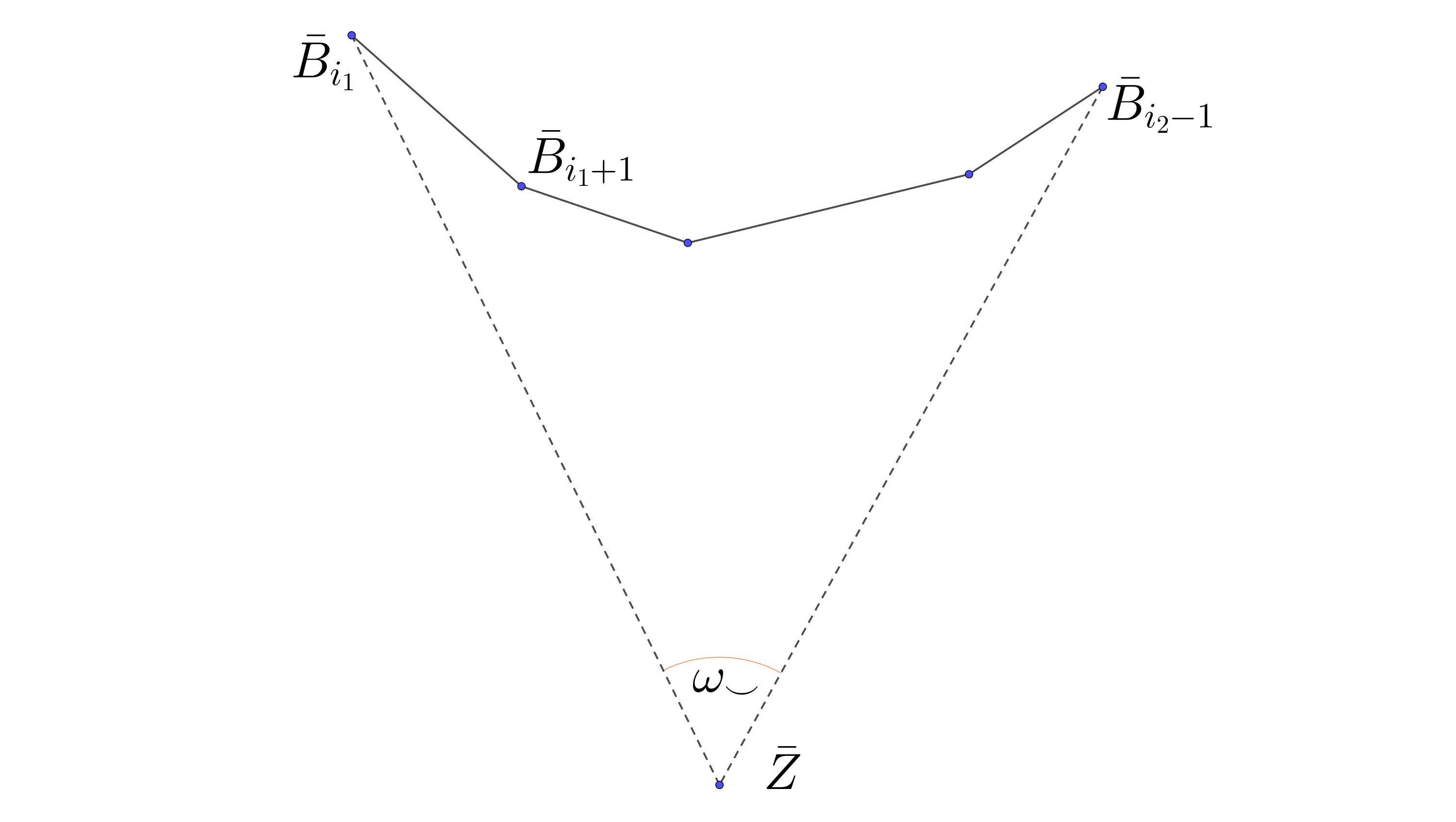
We remark that or . The angle can be seen as follows. Take all orthoschemes for triangles except the first and the last ones, which are singular. The (signed) sum of their angles at is negative and is equal to .
Our plan is to cover the negative polygon by positive triangles constructed from remaining orthoschemes. This will finish the proof: we obtain (5.1) for the sum of all negative pairs with the positive pairs, which we used to cover. All remained orthoschemes are split into positive pairs, for which the inequality also holds. If this is not possible, then we will prove , which is a contradiction.
If we do the same construction as above, but with all , then we obtain a concave polygonal curve seen from under total angle . Then . Indeed, this follows from
that we obtain from the decomposition of into orthoschemes. Note that may be greater than and may be self intersecting when developed to the plane.
Now we return to and start to develop positive triangles to the right from the ray . We note that if , then coincides with , otherwise, lies in the interior of the segment . The new polygonal curve is concave (it is a part of polygonal curve ). As , there are two possibilities: either the new polygonal curve is entirely above (except possibly ) or it intersects transversely.
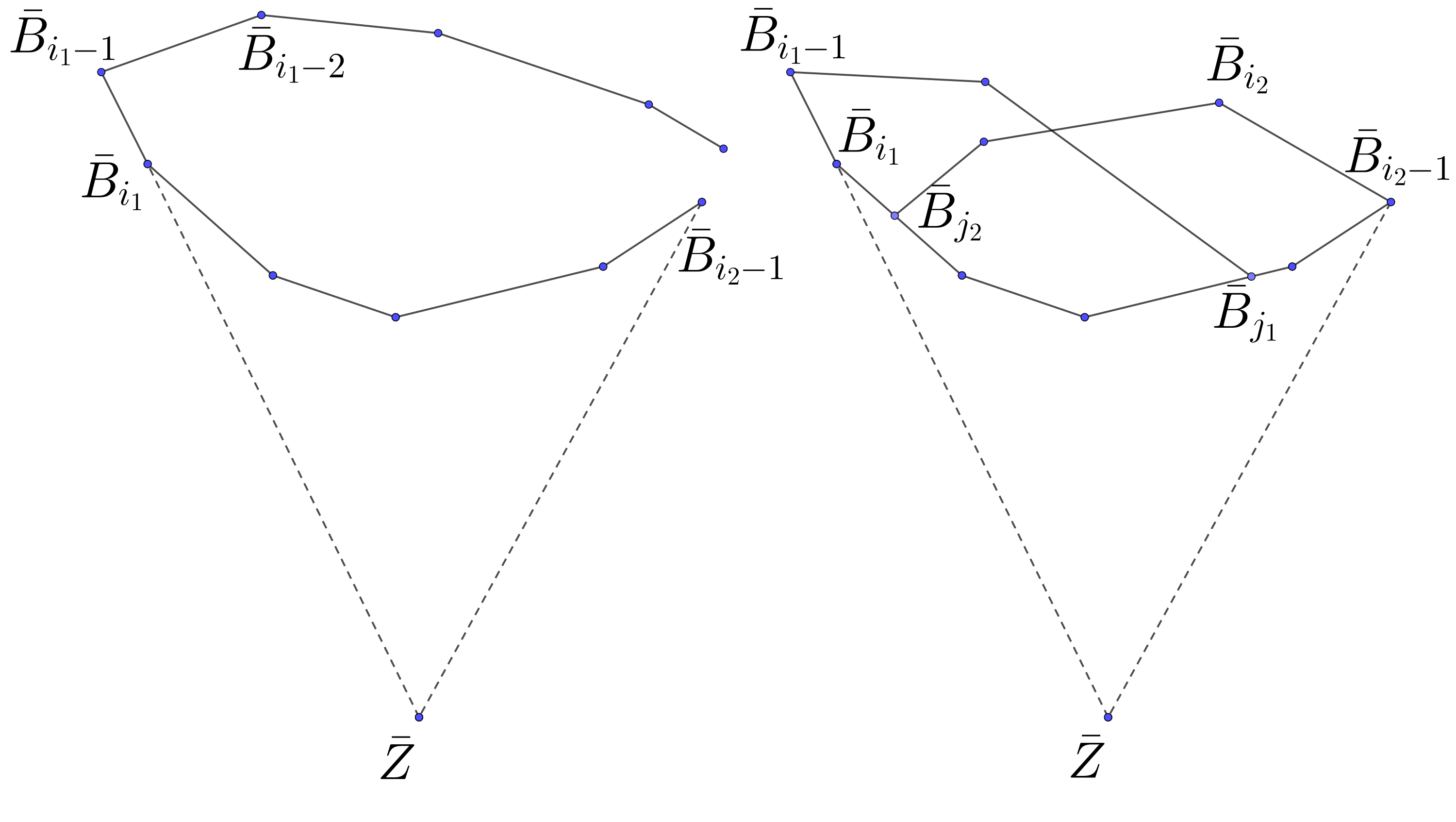
Right: Curves and intersect.
In the first case the proof is finished. In the second case if the intersection point is not a vertex of the upper polygonal curve, then we declare it a vertex. Denote it by . Then we start to develop the triangles to the left from the ray . Similarly, either the new polygonal curve is above or it intersects it. Then declare the intersection point to be a vertex and denote it by .
We need to consider the case when both upper polygonal curves intersect . If is to the left from (or they coincide), then the upper polygonal curves intersect (possibly non-transversely). Let be an intersection point. The polygon is covered by the union of polygons and . They are made from distinct dual orthoschemes because
The last remaining case is when lies to the left from . We denote the polygonal curve by and the polygonal curve by . We will prove that . Our plan is to find points , on the boundary of such that
(1) the angles of both sectors between and are at least ;
(2) .
Indeed, this means that both parts of the boundary between and have lengths greater than . This will finish the proof.
Assume that lies on the segment of (possibly coincides with as a point, however we distinguish then as a vertex of and as a vertex of ). We claim that the angle subtended by is greater than .
Indeed, we consider the polygon formed by , in the tangent plane to the unit sphere at the north pole. Consider the solid cone from the origin over this polygon and take its polar cone. The polar cone intersects the sphere in a polygon consisting of two parts: one is the development of from and the second is a geodesic spherical triangle formed by connecting with via a geodesic segment. The length of this segment is smaller than , hence it is seen from with angle smaller than . This shows that the angle subtended by is greater than .
Similarly, let belong to segment on . Then the angle subtended by is at least .
Now take an arbitrary point of between and . Let it belong to a segment on . We see that the angles of both sectors between and are at least ; similarly for and . It remains to show that either or . We look at three lines: through ; through and through . Due to their location with respect to , either or intersects the shortest segment from to . Without loss of generality, assume that this is . Then the distance from to is smaller than the distance from to . Going to the spherical duals recall that for every the distance from to the geodesic is . Then our conclusion on the lines is equivalent to
which means as desired. ∎
5.1.2 Comparing discrete curvature
Now we investigate how maxima of the discrete curvature behave under some constraints. Let and be the convex polyhedral Fuchsian manifold. By Lemma 2.6.3 maximizes over . Consider . For each define the set
which is non-empty due to Lemma 4.3.1.
The core of our proof of Main Lemma I is the following
Lemma 5.1.2.
The maximum of over is attained at a unique point . Moreover, the map is and satisfies
(1) for each we have and ;
(2) for each we have and .
Here are curvatures in the cone-manifold . The property follows directly from .
Proof.
For reader’s convenience we advise to assume during the first read that is a single point .
First, there is at least one maximum of over . The argument is the same as in Lemma 2.6.3. There are constants such that the supremum of over is equal to the supremum over , which is compact (see Lemma 4.3.3). Indeed, exists due to Lemma 4.6.1, exists due to Lemma 4.6.3.
Let be any of maximum points of over . By we denote the particle curvatures in the cone-manifold .
Claim 1.
For every we have .
Suppose the contrary. Because of Corollary 4.3.7 the height of can be decreased. This deformation stays in and increases due to Lemma 4.4.1, which contradicts to the choice of .
Claim 2.
For every we have .
The proof is the same as of the previous Claim, but we use Lemma 4.3.9.
We obtain that for each and each , we have . For we have . Also if , then there exists such that (we use the fact that the critical point of is unique due to Theorem 2.5.3 and Remark 2.5.4). Corollary 4.3.7 implies that if for some we have , then ; otherwise we can increase while staying in .
For all Corollary 4.3.12 implies that and Corollary 4.5.4 implies that the Hessian of is non-degenerate at .
Take and some . Let us show that there is a unique piecewise -curve such that:
(0) ;
(1) for any , we have (here we write for particle curvatures of the cone-manifold );
(2) for if for some we have , then ; otherwise
Due to this definition, if for some we have , then stabilizes, i.e., for each we have .
First, we see that if is defined for some and , then there exists such that is defined uniquely for all . Indeed, due to Corollary 4.5.4 and Corollary 4.3.12, the Hessian of is non-degenerate at and (note that the can not be positive for as they are non-negative for and once they become 0, they stay equal to 0). Then our claim follows from the Implicit Function Theorem.
Assume that is defined uniquely by conditions (0)-(2) over the interval for some , and for all . The second assumption implies that there exists such that for all . Thus,
By Lemma 4.6.3 there exists such that for all and all we have . By Claim 5 from the proof of Lemma 4.6.1 there exists such that for all and all we get . Then for all we have , which is compact by Lemma 4.3.3. Then there exists a unique point that is a continuous extension of . Moreover, by continuity for all we have . Then the Hessian of is non-degenerate at and . Due to the Implicit Function Theorem, is in some right neighbourhood of .
Thereby, is uniquely defined for all . There might be kink points corresponding to those , when becomes 0 for a vertex .
It follows that either there exists such that or there is such that for all . In the second case as . Then Lemma 4.6.3 excludes this case as it shows that becomes positive for close to .
Thus, there exists such that . We assume that is the maximal with this property. There is such that for all we have . This means that
As it is equal to , then .
Our current aim is
Claim 3.
For all and all we have .
This requires some preparation. Fix that is not a kink point of and define
If , then .
Claim 4.
For each we have .
Indeed, we already saw this for . If , then is identically 0. Lemma 4.5.1 gives
Let be a vertex, where the minimum of is attained over the vertices not from . Because of Lemma 4.3.8 there exists at least one strict edge emanating from , so the sum is non-empty. If , then is easy to see that each summand is negative, which is a contradiction. If , then looking at the sum we see that for every connected with we also have . Repeating this and noting that the graph of strict edges is connected due to Corollary 4.3.12, we obtain a contradiction. This proves Claim 4.
Claim 5.
For every , we have
Define . For every we get
In this sum, is an oriented edge from to and the sum is over all edges starting at . With the help of Lemma 2.4.7 we obtain
Recall that , thus we have . From Lemma 5.1.1 we see
| (5.2) |
If , then we also have
| (5.3) |
Multiplying (5.2) with and subtracting (5.3) from it we write
The coefficients are non-negative. Thus, there exists connected with such that
or equivalently
Consider the maximum of the expression over We obtain that it is attained at points of , where it is equal 1. Therefore, for every we get and Claim 5 is proven.
Let is a kink point of , so for some , is 0 and it is not zero for all larger . Then the right derivative of at is , but the left derivative is smaller. For other the derivatives of remain continuous.
Suppose that there exist such that for some we have . Take to be the largest with this property. We have . However, for all , we get . This gives , which is a contradiction. This proves Claim 3.
From all the above discussion we can see that the maximum point over is unique for all and these points form a -curve that is determined by the conditions:
(0) ;
(1) for any , , we have ;
(2) for any we have
Moreover, for any we obtained and for any we got .
This finishes the proof. ∎
Main Lemma I follows from Lemma 5.1.2 quite easily.
Proof of Main Lemma I.
Let , and be taken from Lemma 5.1.2 (note that from the notation of Main Lemma I is in the notation of Lemma 5.1.2). Define We have . As is the maximal point of over , we see that .
From Lemma 5.1.2 for any we get
Combining this with Lemma 5.1.1 we get
Define . We obtain Rewrite it as
Integrating this we see
Finally, we get
This finishes the proof. ∎
5.2 Proof of Main Lemma II
Main Lemma II states that if we have a sufficiently fine strictly short triangulation of , then we can replace each triangle by a triangle with a swept cone-metric and the same sides and angles. To this purpose it is enough to treat each triangle separately. We summarize our main definitions restricted to a single triangle:
Definition 5.2.1.
By a (topological) triangle we mean a topological disc with three marked points at the boundary called vertices. By a metric on we always mean a metric such that the boundary is geodesic except (possibly) the vertices.
Cone-metrics or CBB() metrics on are defined naturally. We call a cone-metric on convex if, in addition to the condition for the interior points of , also the angles of the vertices of are at most . One can see that this requirement holds for convex triangles in CBB() metrics (Definition 2.1.4).
A metric on is called short if the sides of are shortest paths and the angles of vertices are strictly smaller than . It is called strictly short if, in addition, the sides are unique shortest paths. A cone-metric on is called swept if . Here we note that by we mean the set of interior singularities of , i.e., we do not include the vertices of in . Metric on is a sweep-in of metric if is swept and has the same side lengths and angles in and .
Main Lemma II follows from two lemmas:
Lemma 5.2.2.
There exists an absolute constant such that if is a convex cone-metric on a triangle with and , then there exists a unique sweep-in of on .
Lemma 5.2.3.
There exists an absolute constant such that if is a strictly short CBB() metric on a triangle with and , then there exists a unique sweep-in of on .
The plan is first to prove in Subsection 5.2.1 the existence in Lemma 5.2.2 via the curvature merging process. We also give some quantitative estimates on that will be crucial further in the proof of Main Lemmas IIIA-B. Next, in Subsection 5.2.2 we prove the uniqueness in both lemmas. To this purpose we only need to prove that a swept convex metric on a triangle is determined by side lengths and angles. The proof relies on elementary geometry. Last, in Subsection 5.2.3 we prove the existence in Lemma 5.2.3 with the help of approximation by cone-metrics. Note that the condition on to be strictly short in the statement of Lemma 5.2.3 seems to be non-essential. It is used to avoid some annoying degenerations that we want to exclude from the present manuscript in order to simplify the exposition.
5.2.1 Curvature merging
The main proof idea of Lemma 5.2.2 is that we can take two cone-singularities, cut the metric along a geodesic connecting them and glue-in there a piece of a hyperbolic cone so that the number of cone-singularities is reduced. The main difficulty is that we can not do this in all circumstances. In order to perform this operation, the length of the geodesic and the curvatures of the singularities should satisfy some mutual conditions. Hence, we should control carefully what happens with the metric on each step in order to be able to perform the next one.
We start from two simple lemmas on hyperbolic triangles.
Lemma 5.2.4.
Let and define
Then for any numbers and such that there exists a hyperbolic triangle with , and . Moreover, .
Proof.
Suppose that the triangle exists. Write the dual cosine law for :
| (5.4) |
One can prove that exists if and only if the right hand side is in the range of cosine of a non-zero angle, i.e., it belongs to . Due to elementary trigonometry, the lower bound is always true. We are interested in , i.e., when the right hand side of (5.4) is less than 0.
Let us fix and fix the sum of and . Then if one considers the right hand side of (5.4) as the function of , by taking the derivative it follows that the right hand side is maximized when . Now let us check what is the value of making the right hand side zero. It is easy to compute that
This discussion shows that for any such that the right hand side is smaller than zero, so the triangle exists and . It remains only to note that decreases as increases. ∎
Lemma 5.2.5.
Let be a hyperbolic triangle with sides and angles respectively such that . Then
Proof.
Define
We have
We have . From the concavity of cosine over we obtain
From this we get
Note that and . Therefore,
It follows that
∎
Fix and choose from Lemma 5.2.4. Then choose such that
| (5.5) |
After that we choose such that
| (5.6) |
Now we formulate and prove a quantitative version of the existence part of Lemma 5.2.2:
Lemma 5.2.6.
Let be a convex cone-metric on with and . Then there exists a sweep-in of on such that
Proof.
Put , . At first step take two points and connect them by a shortest path .
Consider the hyperbolic triangle such that
We have
Thus, Lemma 5.2.4 implies that exists and is its greatest side.
We take two copies of and glue isometrically the sides corresponding to and . We call the obtained figure a bigon and denote it by . It has the piecewise geodesic boundary consisting of two segments equal to , two kink points at the boundary, which we continue to denote by and abusing the notation, and a conical point in the interior, which we continue to denote by .
Cut along . Glue isometrically the boundary of with the boundary of the cut: the vertex is glued with , is glued with . Denote the resulting topological space by and the induced path metric . Since now we consider as a subset of . We have a natural map
which is a local isometry with respect to metrics , .
We identify with its -image. The point will be also denoted by . Then
Claim 1.
The map does not decrease the distances.
Indeed, let . Connect them by a shortest path in . If it does not intersect , then the distance between them did not decrease. If it intersects , then the intersection is a segment. This is because of the strong non-overlapping property (see Section 2.1). Let the shortest path intersect the boundary of in points such that is closer to and is closer to . See Figure 10. Choose points such that
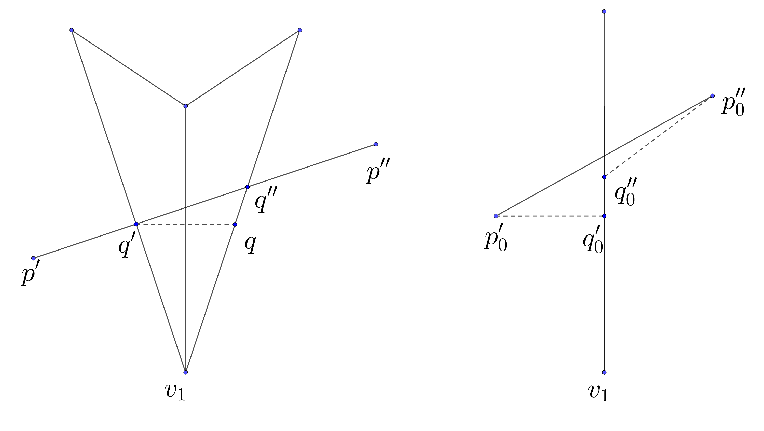
Without loss of generality we assume that lies between and . Then choose a point on the boundary of between and such that . It is clear that . Define , . Then
Claim 1 is shown. As a corollary we get
Claim 2.
Now we need to show an upper bound.
Claim 3.
Indeed, consider in two triangles and sharing the edge , each is isometric to the triangle . As , the point belongs to the interior of the triangle .
Let be the (unique) shortest path connecting and in . Cut along and consider the developing map
One can see that it does not decrease the distances. Then
Note that and
Consider and . Connect them by a shortest path. Let it intersect the boundary of in a point with -image in . In the triangle draw the segment through , which cuts off equal segments from the segments and . Consider its intersection point with and let be its preimage under . Let be a point such that and See Figure 11. Then
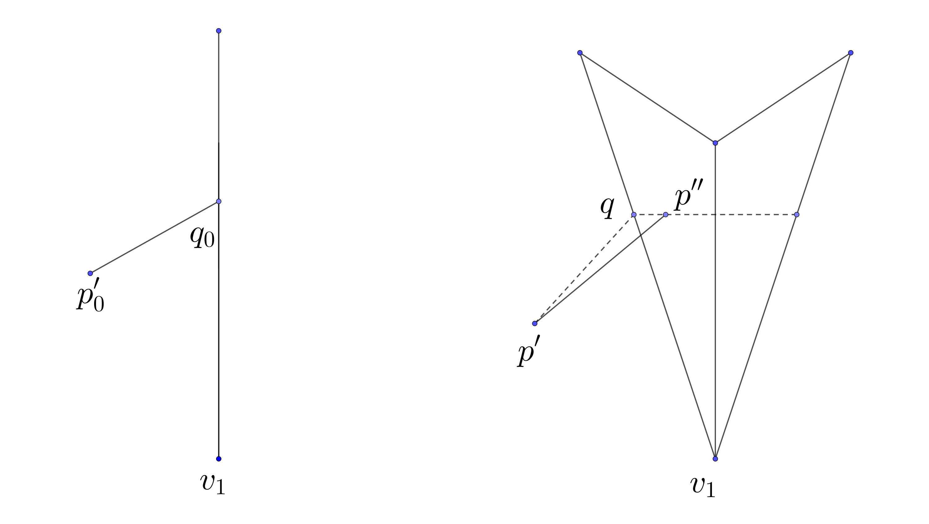
Now we consider . Let and . If , then all shortest paths connecting and in intersect . Consider an arbitrary shortest path between and . Let it intersect at the point . We consider the points at the borders of such that . See Figure 12. Then
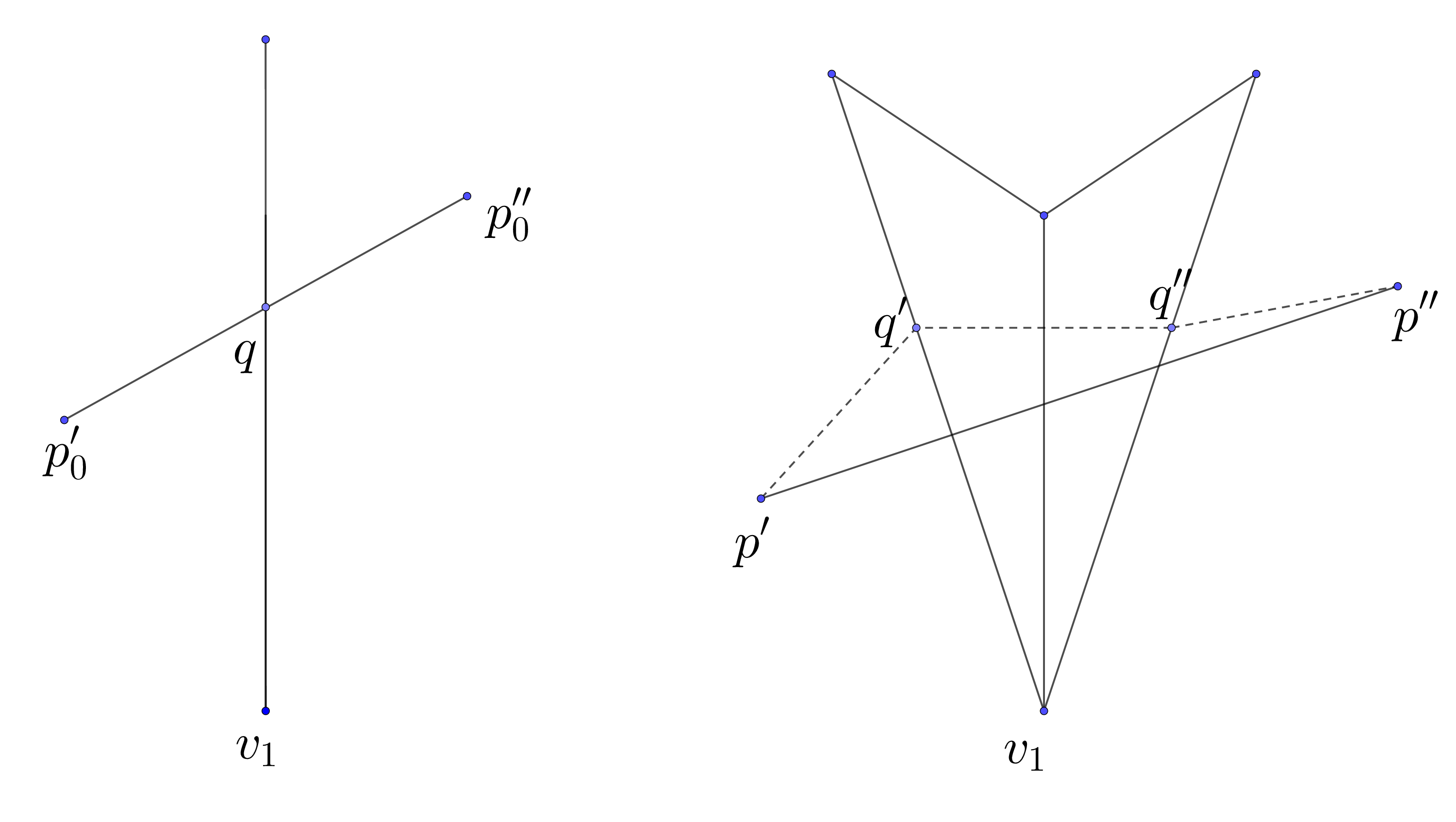
This finishes the proof of Claim 3.
Claim 4.
Indeed, the lower bound is trivial, the upper is just Lemma 5.2.5 applied to triangle .
From Claim 4 we obtain
We continue the process of merging the curvature by gluing new bigons. At every step we take the point that we obtained after the last step, take another conical point and cut the metric along a shortest path connecting both points. Let us check that there always exists a bigon to glue in the cut.
To this purpose we show by induction that after steps
| (5.7) |
Assume that these bounds hold. Let be distinct from . Connect them by a shortest path . Note that and . We have
Then Lemma 5.2.4 shows that the bigon exists to glue with the cut along . We glue-in the bigon and obtain a new metric space and a local isometry . We identify in with its -image in . Let be the interior vertex of . Then
The proofs of Claim 1–4 remain to be valid. (To repeat the proof of Claim 3 we use that the boundary segments of are greater than the distances from boundary vertices to the interior vertex.) From these Claims, (5.5), (5.6) and the induction hypothesis we show
Thus, we established the induction step for (5.7). Finally we obtain a metric space with just one conical point in the interior. As both , are triangles, we may consider as a metric on . The side lengths and angles do not change during the process. Thus, we obtain a sweep-in of on . From (5.5) and (5.7) we get and
∎
Now we make a brief sidestep from metrics on to metrics on . We claim that if we perform the sweeping process described in this section for each triangle of , then the diameter of the resulting metric can be estimated in exactly the same way as for a single triangle. In other words, we state
Lemma 5.2.7.
The existence here follows from Lemma 5.2.6 and the uniqueness will be proven in the next section. Thereby, what we remark now is the diameter estimate. The proof is exactly the same as the proof of similar bounds in Lemma 5.2.6. We only need to note that proofs of Claim 1, Claim 3 from the proof of Lemma 5.2.6, which are responsible for these bounds, work without changes if instead of points in we consider points in .
5.2.2 Swept triangles
Definition 5.2.8.
Since now we call a metric space , where is a triangle and is a swept metric, a swept triangle. It is called convex if is convex. It is called strict if and the curvature of the conical point is positive. Note that a strict swept triangle might be non-convex: this happens if some boundary angles are greater than .
Let be a swept triangle. We also denote it as , where are vertices of and is the interior cone-point of . In case we assume that is a marked point in the interior of , i.e., a swept triangle is always a triangle with a marked point inside. By denote the length of (we assume that are enumerated modulo three) and by denote the angle . We naturally call the side lengths of and its angles. There are unique geodesics from to each vertex. By denote the length of the geodesic and by denote the sector angle . One can see that .
Clearly, a swept triangle is uniquely determined by , (up to isometry). This gives us a parametrization of the set of strict swept triangles up to isometry by the following subset of :
We prove the uniqueness of a sweep-in in Lemmas 5.2.2, 5.2.3. It is easy to see that if a swept triangle has the side lengths and angles coinciding to the side lengths and angles of a hyperbolic triangle, then it is isometric to this hyperbolic triangle. The rest follows from
Lemma 5.2.9.
A strict swept triangle is uniquely determined by the side lengths and angles (up to isometry)
Proof.
We show that the distances in a strict swept triangle are uniquely determined by the side lengths and angles. This also shows that are uniquely determined, which implies the claim.
Cut along the geodesic . Develop it in . Let be the resulting polygon. One can show that it is not self-intersecting even if some boundary angles are greater than .
The side lengths , , and the angles and determine the polygonal line in up to isometry. The point belongs to the perpendicular bisector to segment . We can see that as moves along this bisector, the sum of angles and changes monotonously. Then there exists no more than one position where this sum is equal to the angle . This finishes the proof. ∎
Consider the map , which associates to a strict swept triangle the 6-tuple of its side lengths and angles, i.e.,
Lemma 5.2.9 states that this map is injective. Clearly it is continuous, thereby by the Brouwer Invariance of Domain Theorem we get
Corollary 5.2.10.
The image is open and is a homeomorphism onto its image.
The map will be used prominently in the next subsection.
5.2.3 Sweeping-in CBB() metrics
As we wrote before, the proof of the existence in Lemma 5.2.3 is done via an approximation by cone-metrics. Assume that is a triangle with a CBB() metric. Let be a sequence of convex cone-metrics converging to . There is a sweep-in for each metric . We need to investigate the convergence of swept triangles . It might happen that such a sequence diverges. For instance, it might happen that some in the limit. The tough part of the proof is to show that such degeneracies can not happen when converges to a CBB() metric.
The approximation can be done as in Subsection 3.3. To this purpose first we need to realize on a convex surface. This can be done with the help of Alexandrov’s gluing theorem and Alexandrov’s realization theorem:
Theorem 5.2.11 (The gluing theorem).
Let and be two surfaces with boundaries and CBB() metrics. Let be an isometry (it is possible to consider only some boundary components of ). Then the gluing of and along is a CBB() metric space.
A proof is identical to the CBB(0) case proven by Alexandrov in [5, Section VIII.1]. Another proof in the CBB() case for arbitrary dimension can be found in [51].
Theorem 5.2.12 (The realization theorem).
For every CBB() metric on there exists a convex body such that is isometric to the boundary of .
The proof is also identical to the CBB(0)-case [5, Section VII.1, Theorem 1]. An explanation of differences between CBB(0) and CBB() cases is given in [5, Section XII.2].
Now consider a convex body . Let its boundary be identified with a CBB() metric space . Similarly to Subsection 3.3, we consider a sequence of -dense sets with . Let be the convex hull of . Pick a point for all . The metrics of can be pulled back to convex cone-metrics on with the help of central projection from .
Lemma 5.2.13.
Let be a strictly short triangulation of . Consider a sequence of finite -dense sets with such that all of them contain and none of them contains a point in the interior of an edge of . By denote the metrics on defined as above.
Then converge to uniformly and the triangulation is realized by infinitely many . Moreover, the realizations can be chosen so that they are short and for every triangle of we have (after taking a subsequence)
(1) ;
(2) ;
(3)
A proof of Lemma 5.2.13 can be done exactly in the same way as our proof of Lemma 3.3.6. Instead of distance functions to the lower boundary one should use the distance function to the point . We do not provide here a proof of Lemma 5.2.13. We note that if we want to prove only Main Lemma II, then it is enough to prove the existence of the sweep-in only for metrics coming from strictly short triangles on the upper boundary of a convex compact Fuchsian manifold. In this case we may just use below Lemma 3.3.6 instead of Lemma 5.2.13. However, in a more general Lemma 5.2.3 we do not know if the triangle comes this way and we use Lemma 5.2.13 to overcome this.
Now we turn to a triangle with a strictly short CBB() metric . Take two copies of and glue along the boundary. We obtain a metric on the 2-sphere . Theorem 5.2.11 implies that it is CBB(). Two copies of in form a strictly short triangulation of the latter. We fix an inclusion .
By Theorem 5.2.12, there exists a convex body with boundary isometric to . In order to prove Lemma 5.2.3 we need to consider triangulations of . Let be a strictly short triangulation of with no additional vertices at the edges of . Transfer it to via . Together with the second copy of in it forms a strictly short triangulation of . Now we can approximate by cone-metrics realizing with the help of Lemma 5.2.13. After cutting off from these metrics the redundant triangle of , we obtain approximations of realizing . In other words, we get
Corollary 5.2.14.
Let be a strictly short triangulation of . There exists a sequence of convex cone-metrics on such that they converge uniformly to , all of them realize by short triangulations and for every triangle of we have
(1) ;
(2) ;
(3)
Now we are ready to prove Lemma 5.2.3.
Proof of Lemma 5.2.3.
It remains only to prove the existence for metrics that are not cone-metrics.
Let be an arbitrary positive number and be from Lemma 5.2.4. Take , satisfying (5.5) and (5.6). Define as the minimum of , . Let be a short CBB() metric on with , as in the statement of Lemma 5.2.3. If happens to be the 6-tuple of side lengths and angles of a hyperbolic triangle, then we just let to be the metric of this triangle. Consider the other case.
Corollary 5.2.14 shows that there exists a sequence of convex cone-metrics on such that , and . Moreover, we can demand that are not 6-tuples of side lengths and angles of hyperbolic triangles.
For each by Lemma 5.2.6 we construct a convex cone-metric on such that is a convex strict swept triangle and , so . (Recall the definitions of and the map from Subsection 5.2.2.) It follows that We need to understand what happens in the limit. Define . By and we denote the respective components of .
We claim that after taking a subsequence converges in . Indeed, otherwise for some we have . This can not happen because Lemma 5.2.6 says that . Let By , we denote the respective components of . If , then , so there exists a convex swept triangle with side lengths and angles equal to those of and the proof is finished. It remains to assume that and consider different types of degeneracies that can happen with . We divide them in the following cases:
(i) for some ;
(ii) for at least two ;
(iii) for one ;
(iv) and for all ;
(v) for some , but and for all .
Case (iii) turns out to be the most complicated. So first we rule out the four others.
(i) Let . Consider a strict swept triangle like in Subsection 5.2.2 with . Then for every there exists such that if , then either or or . Now take smaller than the length of any edge of and than the difference of and any angle of . Choose for this . For sufficiently large we see that all . Thus, .
(ii) Let . Consider a strict swept triangle . For every there exists such that if , then . Take smaller than the length of any edge of . Choose for this . For sufficiently large we see that either or is greater than . Thus, either or is greater than 0.
(iv) In this case has the side lengths and angles of a hyperbolic triangle.
(v) Let . Consider the convex quadrilateral with sides , , , and angle between the sides of lengths , . The angle of is equal to the angle of this quadrilateral between the sides of lengths , . Then is smaller than the respective angle in the comparison hyperbolic triangle with lengths , and . This contradicts to the Toponogov globalization theorem (see Section 2.1) and the condition that sides of are shortest paths.
(iii) If , then has the side lengths and angles of a hyperbolic triangle. This can be seen from approximating by cone-metrics as above and noting that converges to . So from now assume that . The idea is the following. If and is any cone-metric sufficiently close to , then the respective component of is sufficiently small. However, we are going to construct arbitrarily close convex cone-metrics to , for which is bounded away from zero. This is done by paying the attention to how we do the approximation. Subdivide into several triangles so that one of them contains almost all curvature and is not adjacent to the vertex of . Then we find a cone-metric close to realizing this new triangulation. When we merge the curvature inside in , the resulting swept triangle does not depend on the process of merging. Hence, we can first merge all curvature inside “the biggest part” of and then all other curvature. We can show that the resulting conical point after the final merging is not close to .
Now we proceed to the details. Let . Denote the vertices of by , , and the respective edges by , , . Fix and choose points and at distance from . Connect with and with by shortest paths. If there are several shortest paths from to , then we choose the one that makes the smallest angle with at (it is easy to see that this determines the shortest path uniquely). Note that except endpoints it is contained in the interior of as otherwise it has to be contained in the boundary and then the angle of at is . Similarly choose the shortest path from to .
Let the chosen paths intersect in the point . By and we denote the segments from to and respectively. See Figure 13. It clear from the definitions that geodesics in a CBB() metric do not pass through points with . Therefore, . Let be the (open) region bounded by , , , and be the (open) triangle bounded by , and . Define
We have . If , then . The intersection of all is empty. Thus, one can see that tends to zero as tends to zero. We choose such that
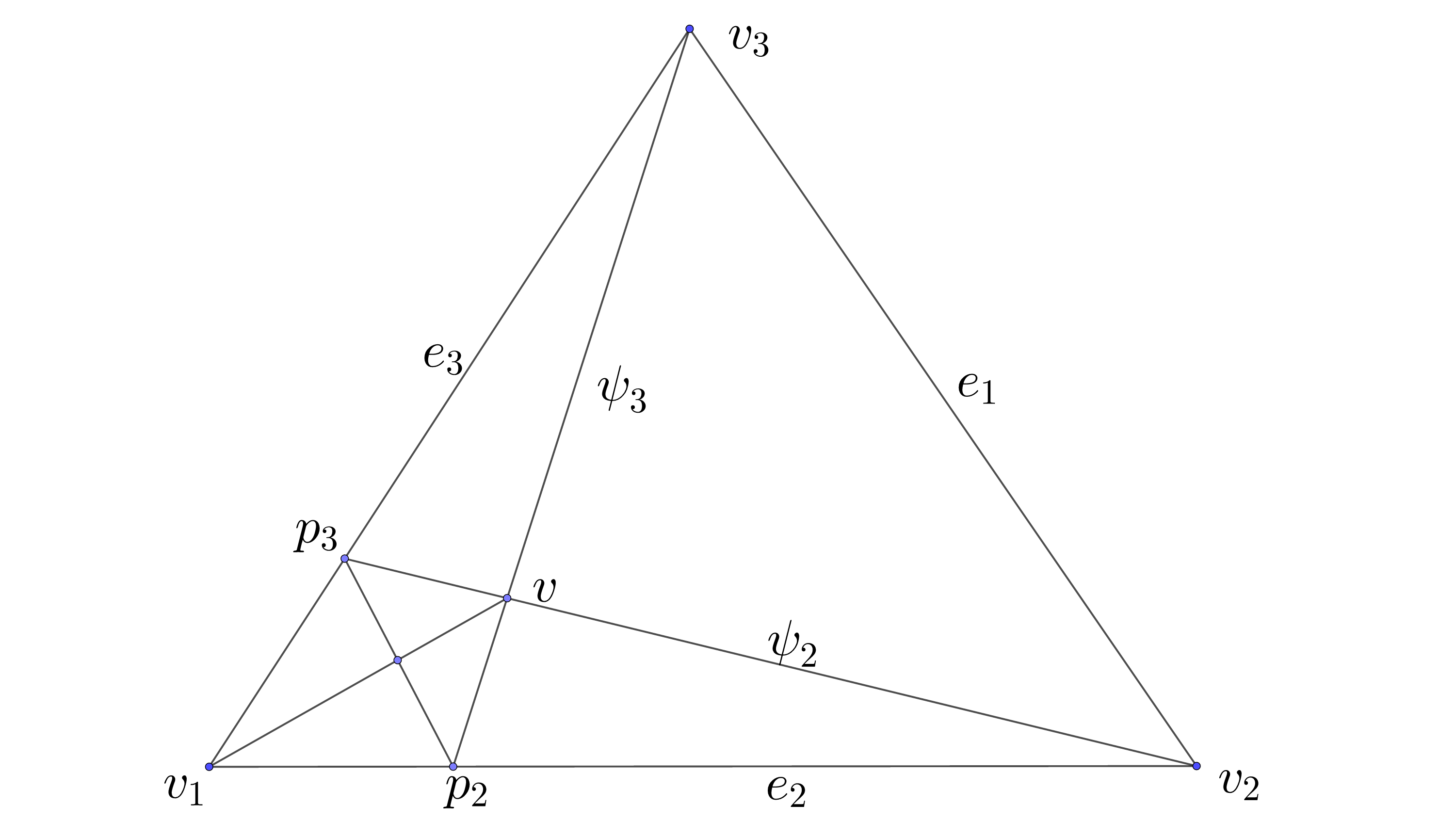
From now on we denote , , and by , , and . Also we define
All sides of the triangle are unique shortest paths due to the strong non-overlapping property. It is very easy to extend our current decomposition of to a strictly short triangulation. To this purpose we just draw two diagonals in the quadrangle . From the strong non-overlapping property, all edges of the obtained triangulation are unique shortest arcs. Therefore, we obtain a strictly short triangulation of containing (angles are less than as no two geodesics can form zero angle, the convexity of triangles follows from the convexity of ). Due to Corollary 5.2.14 there exists a sequence of convex cone-metrics on converging to uniformly and realizing . Define
Here by , we mean their realizations in . From Corollary 5.2.14 we can choose so that , and as goes to infinity. From the uniform convergence one can get .
Now choose such that
| (5.8) |
Here , are angles at the vertex in , respectively and is the distance from to the cone point in the sweep-in of . Since now we denote , , and by , , and .
By Lemma 5.2.9 we see that if we merge all curvature inside in one point (by gluing bigons), then the resulting swept triangle does not depend on the choice of a merging algorithm. Lemma 5.2.6 says that its diameter is smaller than . Claim 2 of Lemma 5.2.6 shows that after each merging the diameter of is not decreasing, therefore is an upper bound on the diameter of during the whole process.
First, we merge all curvature inside to point . By Claim 1 of Lemma 5.2.6 the distance from to is at least . Now we merge all curvature in to a point . We note that is not convex, hence we do not expect that stays in . Let be the resulting cone-metric on . We would like to glue a bigon along the shortest path connecting and . From Claim 4 of Lemma 5.2.6 we see that and . Then from inequalities (5.5) we get . Together with , it follows from Lemma 5.2.4 that the last bigon exists.
Let be the resulting curvature point, be the resulting metric and be the base of perpendicular from to the boundary segment of the glued bigon that is intersected by a shortest path from to . See Figure 14. Then .
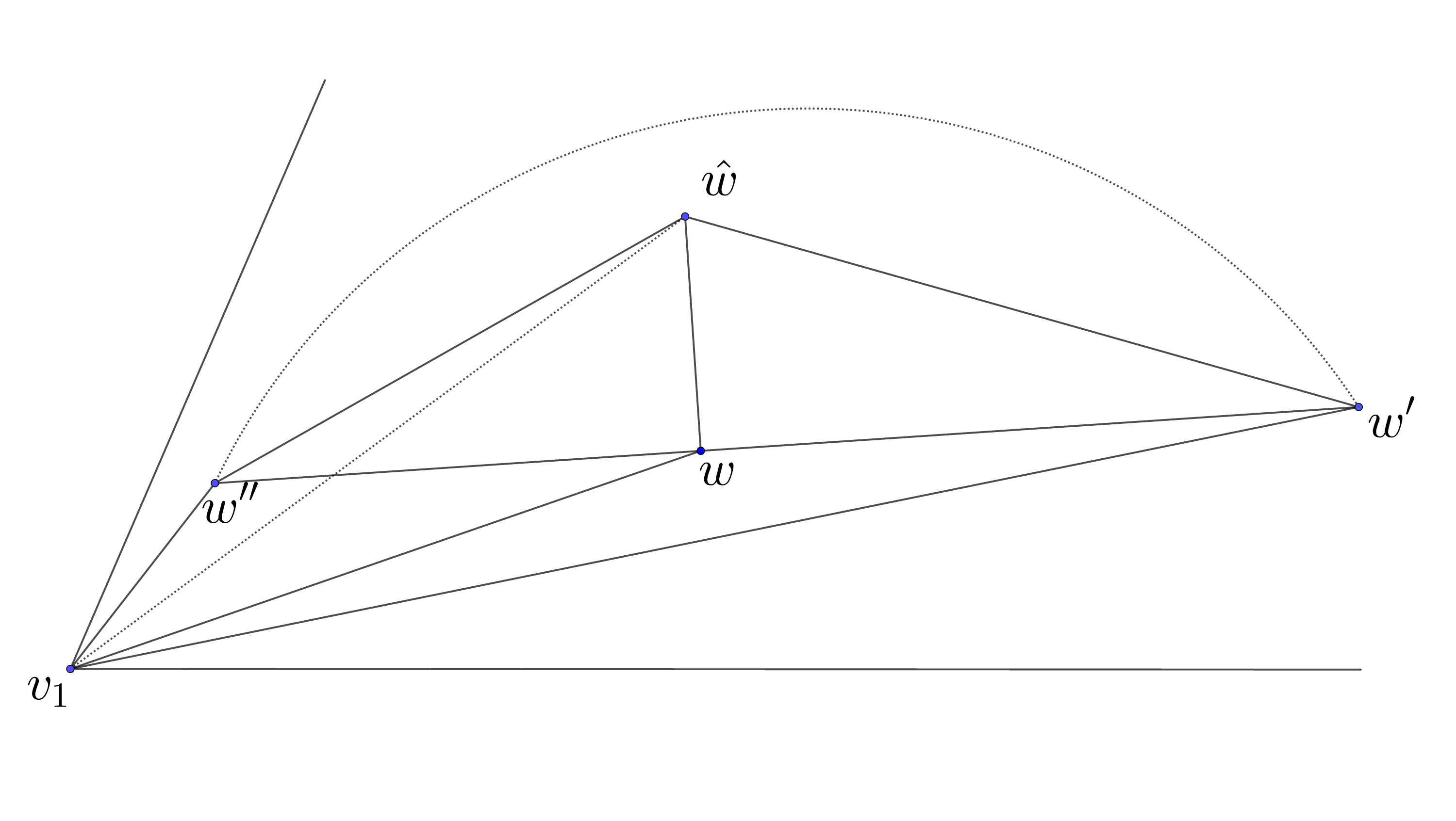
Note that By the choice of there is the upper bound (5.8) on . We are going to obtain a contradiction with this bound. We consider two cases. First, suppose that . Then we claim that
Indeed, elementary trigonometry shows that for each hyperbolic triangle with and , we have the hyperbolic tangent of the distance from to the segment is at least . We apply this to the triangle . This contradicts to (5.8).
In the other case, we suppose . Write
Now we bound . Recall that .
Recall that
Also due to our assumption.
In total we get
This gives the last contradiction with . It follows that and the proof is over. ∎
5.3 Proof of Main Lemmas III
The rough idea of our proofs of Main Lemmas IIIA-C is as follows. Assume that we have a path of metrics parametrized by and a convex Fuchsian cone-manifold . We want to transform this cone-manifold continuously along the path so that (1) heights of the vertices can move only in one direction (up); (2) we control the change of discrete curvature (for our purposes it is enough to control it also only in one direction). There are two aspects impacting the discrete curvature: the change of heights and the change of the upper boundary metric. A great observation is that we can move up only vertices with positive curvature. This always increases and it remains to bound the change of under the metric change. Another idea is that we may consider separately two types of small deformations of : (1) transform heights with fixed boundary metric (Section 5.3.1); (2) transform boundary metric with fixed heights. Our transformation is decomposed virtually into a discrete process. A “continuous induction” argument (Lemma 5.3.13) allows us to combine this into a continuous one. We note that for technical reasons we can control efficiently only heights of vertices with . Thereby, we pay plenty of attention to the change of the singularity set .
Last, we make remarks on metric paths . For proofs of Main Lemmas IIIA-B we turn the operations of gluing/cutting a bigon from the proof of Lemma 5.2.6 into continuous processes. This is done in Subsection 5.3.2. For our proof of Main Lemma IIIC we introduce a process of dissolving/creating cone-points of small curvature. This is described in Subsection 5.3.7. The rest of the proof of Main Lemma IIIC follows from an indirect transformation based on a study of local properties of the space .
5.3.1 Changing heights with fixed boundary
Recall that and denote the sets of convex cone-metrics on with and with respectively.
Lemma 5.3.1.
Let be a convex Fuchsian cone-manifold with . Define as the set of convex cone-metrics such that for every ,
Then there exist and such that:
(1) for every ;
(2) ;
(3) for every metric .
Proof.
Consider the face decomposition . By a triangle of we mean a triangle of a triangulation compatible with such that . Recall that due to Lemma 4.3.2, there are finitely many triangulations compatible with and, therefore, finitely many triangles of .
First we see that in some cases we can simply take . Consider a triangulation compatible with and the Fuchsian cone-manifold . It might happen that is not convex. Let us use the flip algorithm described in Lemma 4.3.9: take an arbitrary concave edge and flip it. Provided is sufficiently small, strict edges of remain strict in all intermediate cone-manifolds during the algorithm and, therefore, can not be flipped. We refer to the proof of Lemma 4.3.9 for details. Thus, all triangulations that appear are compatible with . We also recall that the extension of the height function is pointwise non-decreasing during the process and is increased at least in one point. Hence, the algorithm can not run infinitely.
If every concave edge can always be flipped, then the algorithm terminates with a triangulation such that the Fuchsian cone-manifold is convex. Recall from the proof of Lemma 4.3.9 that there are two types of edges that can not be flipped. Motivated by this we define the notion of obstructive vertices.
(a) A vertex is called obstructive of type I if is isolated and there exists a triangle of with two edges adjacent to glued together. We say that is associated to .
(b) A vertex is called obstructive of type II if there exist two triangles and of sharing a flat edge incident to and the total angle of at this edge is at least (it might happen that this edge is incident to twice, then we count only one incidence). We say that and are associated to .
Otherwise a vertex is called non-obstructive. Suppose that all vertices are non-obstructive in . It is possible to choose small enough so in any all vertices remain non-obstructive. The discussion above shows that in this case any concave edge can be flipped, the flip algorithm terminates and we can take .
Now we assume that there are obstructive vertices. Our aim is to find such that properties (1) and (2) from the statement of Lemma 5.3.1 are satisfied and there are no obstructive vertices in .
There might be plenty of triangles associated to an obstructive vertex. We remark that being obstructive of type II is a stronger property than having an angle at least in a face of . Indeed, take a hyperbolic polygon with , and . Glue the sides and . The angle of vertex obtained from and is greater than . However, one can see that it is not obstructive of type II, i.e., for any triangulation of the respective surface, any two adjacent triangles have total angle smaller than at .
Because an obstructive vertex of type I is isolated and , Lemma 4.3.8 implies that (one can see even more that in this case). Lemma 4.3.4 shows that also for an obstructive vertex of type II.
Claim 1.
Let be obstructive of type I, be the associated triangle and be the other vertex of . Then .
Indeed, develop the prism containing as the prism in , where corresponds to , and correspond to .
The lengths and are equal. The distance to the lower plane is the same at the corresponding points of and . It implies that the prism has a plane symmetry with respect to the plane orthogonal to , passing through and the midpoint of . Then the dihedral angles of and are equal to . Hence, is the closest point from the upper plane to the lower. From this we see that .
Claim 2.
Let be obstructive of type II and , be the respective associated triangles. Then there exists a vertex of or such that .
Indeed, develop the prisms containing and as a polyhedron in . Let be the vertex of this polyhedron corresponding to . It has angle at the upper face at least , therefore it lies in the convex hull of other upper boundary vertices. By the convexity of the distance function, one boundary vertex has height strictly greater than .
Together these claims imply
Claim 3.
There exists a triangle associated to an obstructive vertex and containing a non-obstructive vertex.
Indeed, consider the set of pairs , where is obstructive and belongs to a triangle associated with . Take a pair among them such that has the maximum height. Then is non-obstructive.
Now we describe a change of heights satisfying the conditions (1) and (2) of the Lemma such that all strict edges remain strict and at least one new strict edge appears. This new edge is a flat edge of . There are finitely many of them, therefore, the process terminates with a Fuchsian cone-manifold without obstructive vertices.
The deformation is the same as described in Lemma 4.3.9, but it is applied now to the set of obstructive vertices, which is a subset of vertices with positive curvature. Namely, for define by if is obstructive and otherwise. One can see that the argument from the proof of Lemma 4.3.9 works without modifications to show that for small enough we get . Since for every obstructive , this deformation increases .
Consider . It is clear that for sufficiently small , strict edges of remain strict in and non-obstructive vertices remain non-obstructive. By Claim 3 there is a triangle associated to an obstructive vertex that contains a non-obstructive vertex. In the proof of Lemma 4.3.9 it is shown that a flat edge of necessarily becomes strict. ∎
The assumption was essential in our proof of Lemma 5.3.1, but we need also to deal with . In this case we can guarantee the following weaker version:
Lemma 5.3.2.
Let be a convex Fuchsian cone-manifold, . Define as the set of convex cone-metrics such that for every
Then for every there exist and such that:
(1) for every ;
(2) ;
(3) for every metric we have .
Proof.
The proof is the same to Lemma 5.3.1. There is one thing that goes wrong: there can be obstructive vertices of type II with . This tiny aspect appears to be important: when we move such a vertex up, becomes negative due to Lemma 5.3.17 below. Thus, moving up such vertices may produce an unpredictable negative impact on . Nevertheless, we can control it. At each step of moving obstructive points higher (see the end of the proof of Lemma 5.3.1) we can choose small enough such that if decreases, then it decreases by arbitrarily small amount. We have an upper bound for the number of steps (all edges that appear are flat edges of and there are finitely many of them), therefore the decrement of can be kept under . ∎
Now we consider deformations of the boundary metric.
5.3.2 Gluing a bigon continuously
We return to the operation described in the proof of Lemma 5.2.6: modifying a cone-metric by gluing a bigon. We turn it into a continuous process. After this we will learn how to transform a Fuchsian cone-manifold along with gluing a bigon to its upper boundary.
Let , , be a shortest path between and and
| (5.9) |
Here is arbitrary and is taken from Lemma 5.2.4. On choose a point such that
Define . Now we consider as an element of .
As in the proof of Lemma 5.2.6, we consider a hyperbolic triangle such that
Lemma 5.2.4 implies that exists and is its greatest side. Let be the height of from point , so . Then
Define . Note that
| (5.10) |
For every let be the point such that .
Cut along . Glue there a bigon as in Section 5.2.1 consisting of two copies of . We obtain a metric on . The set can be naturally defined in all metric spaces . We associate the remaining point with the vertex of . Thus we get a continuous path of convex cone-metrics parametrized by . Moreover, for each we have . Also note that and .
By we denote the unique shortest paths from to and in each metric respectively. Remark that for any the metric can be obtained from by cutting along and and gluing there the conical 4-gon obtained from two copies of the 4-gon . Treating this operation similarly as in the proof of Claim 1 of Lemma 5.2.6 one can show that the diameter of is non-decreasing with respect to .
Assume that we have a convex Fuchsian cone-manifold . We want to transform it into a convex Fuchsian cone-manifold and estimate the change of .
5.3.3 Changing boundary with fixed heights under gluing a bigon
All the notation is taken from the previous subsection. Here we are going to estimate the change of under a small deformation of the boundary metric with the fixed heights. We do it modulo several quantitative results that we prove separately in Subsection 5.3.4. After this in Subsection 5.3.5 we combine it with the results of Subsection 5.3.1 to get the full deformation.
For a metric on define
Lemma 5.3.3.
Let . Assume that there is
and a triangulation with such that every convex Fuchsian cone-manifold is compatible with . Then
| (5.11) | ||||
Proof.
By denote . As all are compatible with , is a function of the upper lengths for . From Lemma 4.4.1
We have
First we suppose that the edges of changing their lengths over are split into three groups:
(1) edges that intersect once;
(2) edges that intersect once;
(3) edges with as one (and only one) of the endpoints.
We call this case simple. In the general case it might happen that an edge belongs to several types, or intersects or more than once, or has as both endpoints. First we give a proof in the simple case when neither of this happens, and then show how to reduce the general case to the simple one.
We denote the set of edges of each type by , and respectively.
Consider for . Triangulate the bigon in the natural way and extend it to a triangulation in any way. This is possible because of Lemma 2.3.6, which allows to extend any partial triangulation to a full triangulation. Note that for all the metric realizes . In the metric our triangulation degenerates, but this provides no additional difficulties to the discussion below. The deformation can be described easily in the chart as only two edges of ( and ) change their lengths in .
Take . Develop the path of triangles of intersecting in the moment to . The development results in a (possibly non-convex and self-intersecting) triangulated polygon in . See Figure 15. Denote the image of the endpoints of in the development by and . By construction, is in the interior of and intersects each interior edge of its triangulation. Note that a triangle of can be repeated several times in the triangulation of .
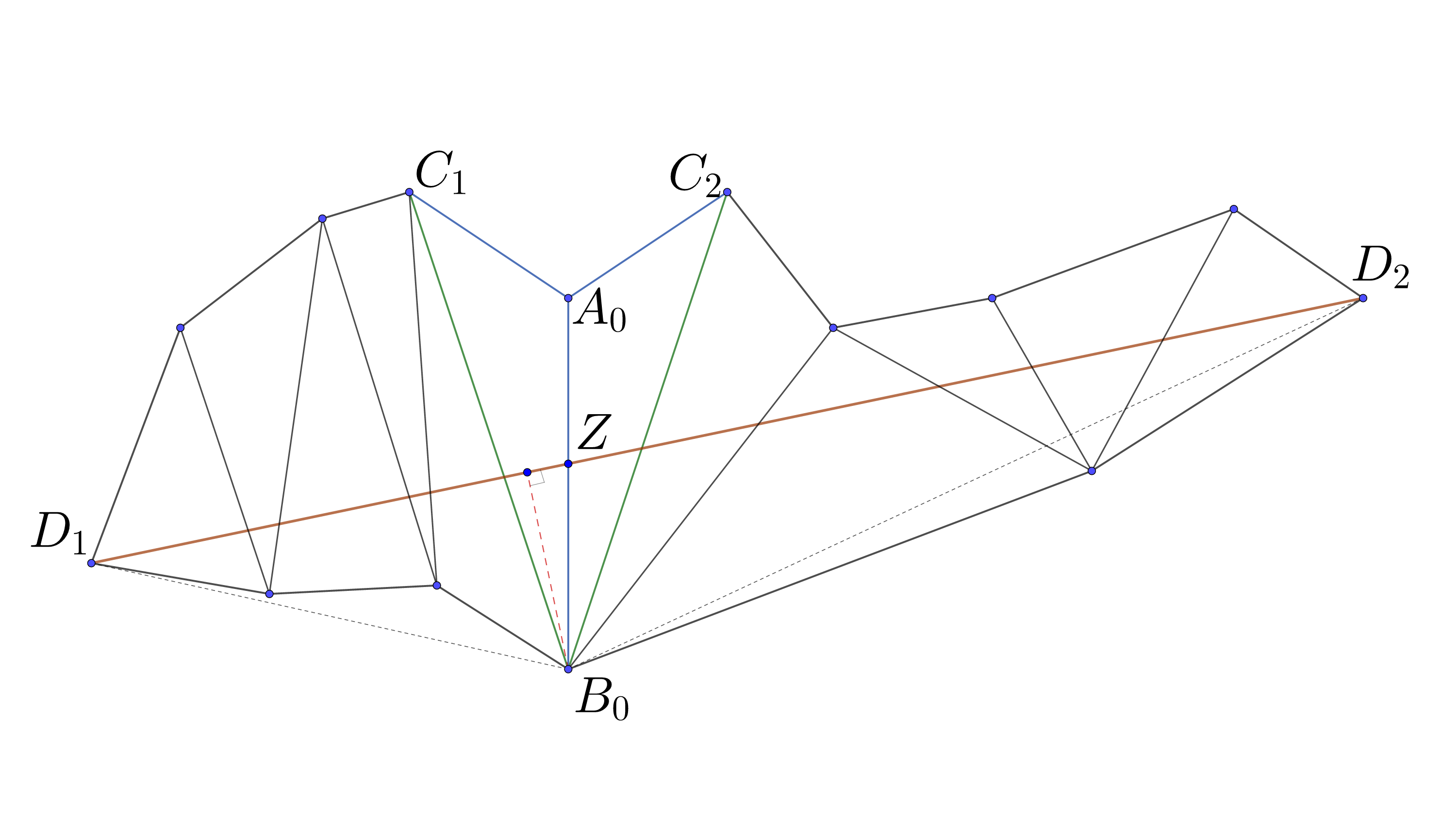
As and the situation is simple, there exists exactly one interior edge of that is the image of under the developing map. Denote its endpoints by and so that corresponds to , to , and by , denote the points corresponding to . Thereby, the triangles and are isometric to the triangle from the bigon , the distances and do not change during the deformation and .
Let be the hyperbolic sine of the length of perpendicular from the point to , be the angle and be the angle . We claim
| (5.12) |
Indeed, differentiating the cosine rule for the triangle we obtain
However, therefore we get (5.12). It is easy to see that , therefore .
Let and intersect in a point . By denote . By denote the smallest angle at which intersects . We have
| (5.13) |
In consider the geodesic ray from the point corresponding to orthogonal to . Let this ray make the angles and with the segments of . Define . Corollary 5.3.5 shows that
Together with Corollary 5.3.6 and Lemma 5.3.9 this gives
Combined this with (5.12) and (5.13) we get
| (5.14) |
Consider the union of all segments connecting points of with their orthogonal projections to . This set is isometric to a convex hyperbolic polygon, which is the union of trapezoids with the angles at the upper boundary equal to (here varies in ). The total length of the upper boundary is equal to . Apply Corollary 5.3.11 and get
| (5.15) |
Here we used for all .
The map is monotone. Substitute in the integral
Now we consider the triangles , embedded in the triangle . Note that and Therefore,
Here we used the concativity of and the convexity of .
In total we get
The same bound holds for the edges of the second type:
Now consider edges of the third type. By Lemma 5.3.7 and Lemma 5.3.8 we have
Recall here that is the total cone angle of in the cone-manifold .
Let . Develop the path of triangles of intersecting in the moment to . Let be the image of under the developing map, be the image of the second endpoint of , be the image of the boundary segment of intersected by .
Consider the moment and develop this path of triangles so that the image of each triangle coincides with its image under the previous development, except the first one, which is developed to . Then , . Note that the angle is not acute, therefore , which implies .
From the triangle inequality we see
Hence, . Then
Summing up all three estimates we get exactly the estimate (5.11). This finishes the proof in the simple case.
Consider the general case, when an edge may intersect each of and several times and in the same time may have endpoints at . We subdivide our exposition further. We suppose now that each edge , when it crosses , intersects either or and then leaves . This means that we exclude the case when after intersecting our edge intersects or vice versa. We call this case semi-simple.
As before, we develop the path of triangles intersecting in the moment to as a triangulated polygon . Orient arbitrarily and enumerate all the triangles of with respect to the orientation. By denote the number of edges in (including the interior edges of the triangulation of ) and by denote their lengths in the moment . The lengths and the combinatorics determine up to isometry. Thus, the length can be considered as the composite function We consider the derivative as the composite derivative
and decompose this sum into elementary deformations, which have types (1), (2) and (3) similar to the edge types in the simple case.
(1) Assume that and are two subsequent triangles of that are the images of under the developing map, and they share an edge that is the image of intersected by . Let be the length of this edge and , be the lengths of the images of (as leaves immediately, the edges of , at the boundary of are the images of ). Then we say that the sum of coordinate derivatives
is an elementary deformation of the first type.
An elementary deformation of the first type is analyzed in the same way as the deformation of an edge of the first type in the simple case. Let be the hyperbolic sine of the length of perpendicular from the image of in to the image of and consider as the function of , which is the angle at vertex in the bigon . Then
(2) An elementary deformation of the second type is defined similarly, but swapping and .
(3) Assume that is the starting vertex of and , are the lengths of the edges of that are the images of and . Then we say that the sum of coordinate derivatives
is an elementary deformation of the third type. Similarly, if is the ending vertex of , then the sum of coordinate derivatives of side lengths of the last triangle also form an elementary deformation of the third type.
As in the case of an edge of the third type, we have
We see that every coordinate derivative
either belongs to exactly one elementary deformation or is equal to zero. Therefore, the total derivative can be decomposed into the sum of elementary deformations.
We do this for every edge of and group elementary deformations of each type together for all edges. Then we decompose the sum
into three summands corresponding to elementary deformations of each type. The integral of each summand is estimated in the same way as in the simple case. This finishes the proof in the semi-simple case.
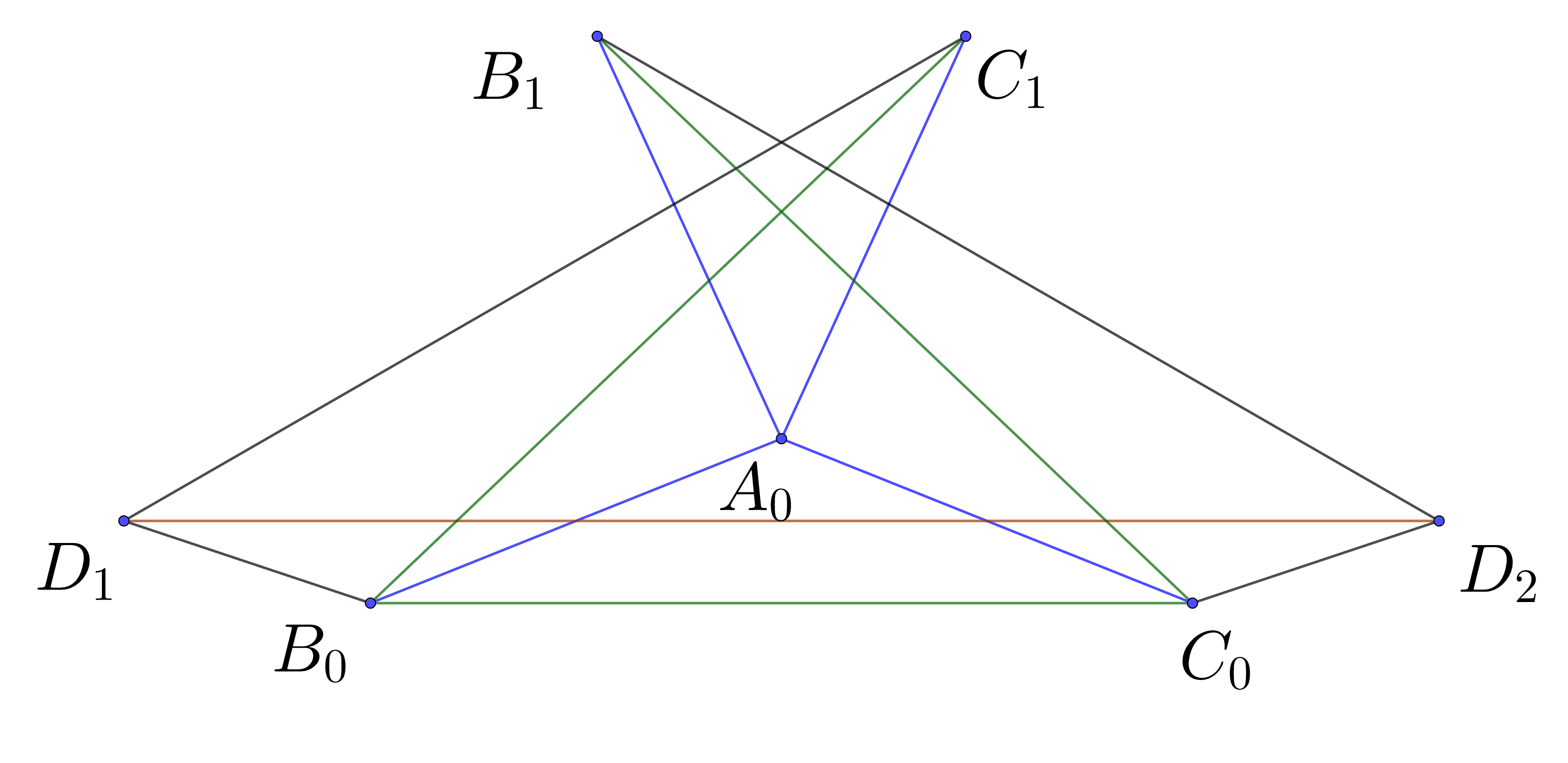
Now we proceed to the last remaining case when, in addition to the previously described events, may enter and cross and then or vice versa. Note that after this needs to leave as otherwise it self-intersects inside . Let the development of in corresponding to this event be the pentagon . It is self-intersecting as the total angle is greater than . See Figure 16. Here and are images of , and are images of . By we denote their lengths. By we denote the angle of at , the endpoint of , and by we denote the angle of at , the endpoint of .
In this case we need to decompose the partial derivatives further. Define
We say that the elementary deformation belongs to the type (1) and belongs to the type (2).
Let be the hyperbolic sine of the length of perpendicular from to the image of , be the hyperbolic sine of the length of perpendicular from . We have , . Thus, it is easy to see that
so indeed , can be treated in the same way as elementary deformations of types (1) and (2) that were defined for the semi-simple case. Hence, the bound for
remains the same and we finish the proof. ∎
5.3.4 Slopes and angle estimates
All results of this subsection are auxiliary for the proof of Lemma 5.3.3 and a similar Lemma 5.3.22 below.
Let be a convex Fuchsian cone-manifold, be a point and be a face triangle containing . Embed the prism containing to . Lemma 4.1.1 says that this prism is ultraparallel. By we denote the image of , by its projection to the lower plane, by denote the common perpendicular between the upper and the lower boundary planes. Define
It is clear that it does not depend on the choice of an embedding and if is contained in a face of , then does not depend on , so we can denote it as We have .
Recall that
Lemma 5.3.4.
For each and a face with we have
Proof.
We claim that there exists a point such that . Indeed, we can assume to this purpose that , i.e, is not a conical point and does not belong to a strict edge, because this does not change . Consider the unit speed geodesic starting from in the direction . Suppose that extends to the distance from (it may not happen in the only case when ends in a conical point before). Let be the point at the distance . Consider the function on defined by
We recall the definition of -function and -concave function from Section 4.2. By definition, is ; is -concave due to Lemma 4.2.1 and coincides with the restriction of to in a neighbourhood of . Then
In the case if ends in a conical point before moving at distance , we can perturb slightly the direction of to avoid this. By the argument above, we obtain such that for some . We can make arbitrarily small and consider a limit point of the set . By continuity of , we have .
The following corollary easily follows after a local development.
Corollary 5.3.5.
Let and be the angle between a geodesic ray from in and the geodesic ray from orthogonal to . Then
The next corollary is just slightly more involved.
Corollary 5.3.6.
Let be an edge of , , be the dihedral angles of in the prisms containing . Then
Proof.
Let be the prism containing with dihedral angle and be the upper boundary triangle of . Embed it to and let be as above. By denote the closest point to on the line containing and by denote its projection to the lower boundary plane. Then is either or and . The only issue is that may lie outside of . Then take any and note that . Apply Lemma 5.3.4 and finish the proof. ∎
Lemma 5.3.7.
Let be a convex Fuchsian cone-manifold. Then for every we have
Proof.
Let and be ultraparallel hyperbolic planes in , and be the closest points, be a point, be its projection to and .
Consider an angle of value in with the vertex . Let be the value of its orthogonal projection to . We claim that
| (5.16) |
First, assume that belongs to one of the two rays bounding and . We call it an angle of the first type. By looking at the spherical link we get
| (5.17) |
Let We have and
for . This proves (5.16) for angles of the first type. We can also see that is monotonously increasing and concave for .
If we have an angle of value that is the union of two angles of the first type, then (5.16) holds by additivity. We call it an angle of the second type.
Let an angle of value be the difference of two angles of the first type of values and . We call it an angle of the third type. Then by concativity of for the projections of these angles we have
Now consider an arbitrary angle at . Let be a line in through orthogonal to . Take the part of our angle that lies on the other side from with respect to and replace this part with its centrally symmetric image in with respect to . This does not change neither the total value of the angle nor the total value of the projection. Now we have at most two angles and each of them belongs to one of the three types described above. Then they satisfy (5.16) and so does the initial angle.
Consider a convex Fuchsian cone-manifold . Subdivide its face decomposition into triangles. For a vertex incident to a triangle let , be the angles of the prism containing in the upper and lower faces corresponding to . We showed that
Thus,
∎
Lemma 5.3.8.
Let be a convex Fuchsian cone-manifold. Then for every we have
Proof.
Consider the spherical link of at . It is a spherical polygon with a conical point of total angle and boundary angles . Then its area is
∎
Lemma 5.3.9.
Consider two half-planes in sharing a line (see Figure 17). Let and , be geodesic rays from making an intrinsic geodesic in the union of and . By denote the (smallest) angle between this geodesic and .
Let be a geodesic ray from in the (convex) dihedral angle spanned by and and be the half plane spanned by and . By , denote the dihedral angles between and , respectively. By , denote the angles between and , respectively. Define . By denote the (smallest) angle between and .
Assume that for some with we have
Then
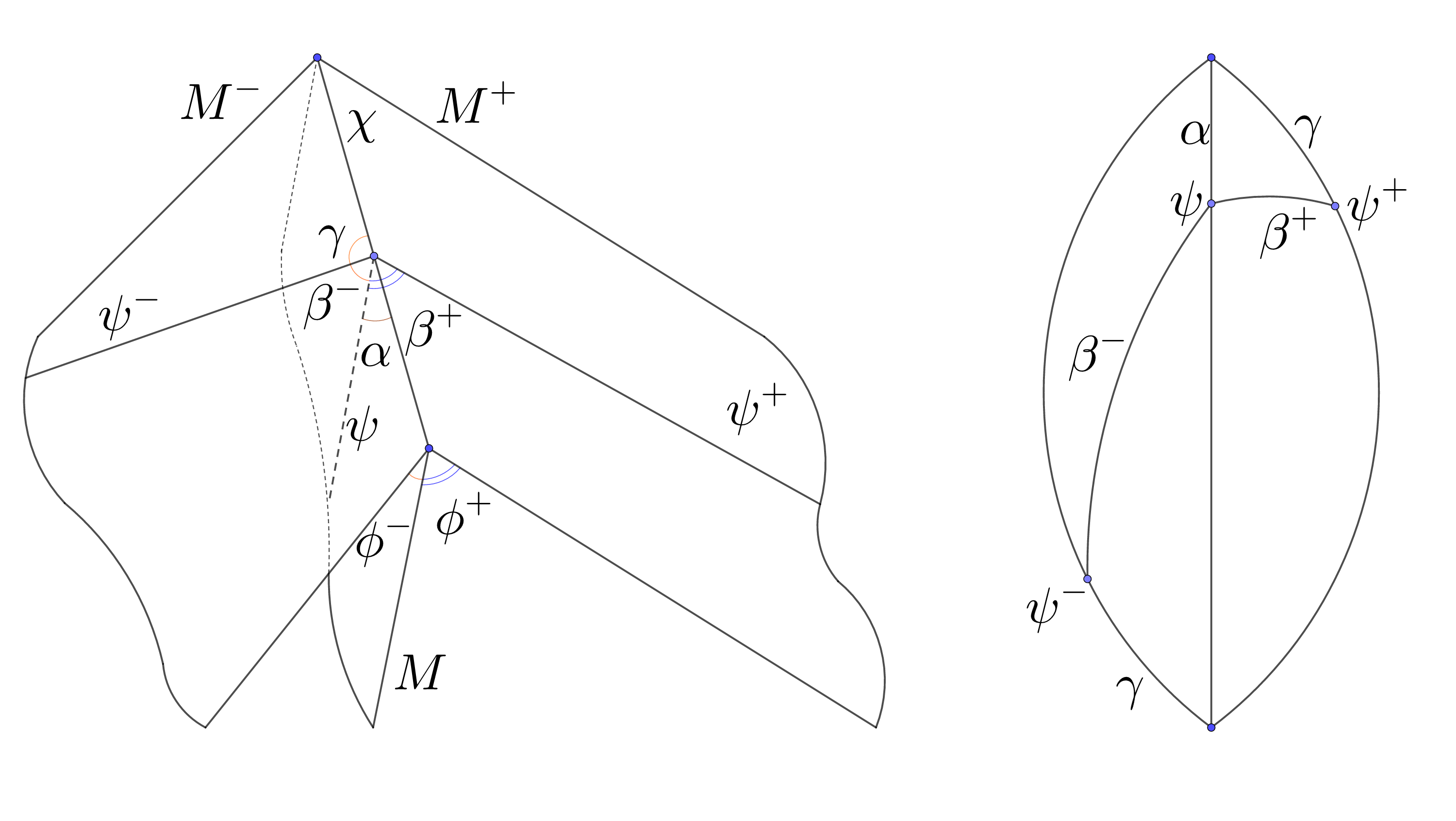
Left: In space. Right: in the spherical link of .
Proof.
We consider the function as the function of , , and and find its minimal value under the given restrictions.
Note that . As , then if and only if . So we assume that .
Consider a spherical section at , so geodesic rays become points and half-planes become half-circles. Assume also that belongs to the spherical triangle with the other sides and (otherwise, switch and ). From the cosine law we get
As , then from elementary trigonometry
with equality if and only if . Thus,
and
Assume that . Fix and consider the function
as a function of . It suffices to prove . Using L’Hopital’s rule we compute the limit of as :
Now we compute its derivative
We see that if is a critical point, then is equal to .
It remains to check what happens as . From elementary trigonometry we have
In total we get
which is equivalent to the desired inequality. ∎
Lemma 5.3.10.
Let be a trapezoid in . Then
| (5.18) |
Proof.
We claim that is enough to prove (5.18) for a right-angled trapezoid. Indeed, if both , are less than , then the trapezoid is ultraparallel and, moreover, can be cut into two right-angled ones. If we know (5.18) for both of them, then it holds also for the initial one. Suppose that . Then we can rotate around until becomes so that the area only grows.
Thereby, it is enough to prove (5.18) for . We use the notation from Subsection 2.4. The area of the trapezoid is . From Corollary 2.4.5 we have
Therefore, the area of the trapezoid is less than . Consider the function . We have
As , it follows that for . This finishes the proof. ∎
Corollary 5.3.11.
Let be a convex polygon in with , be the angle and be the sum of lengths . Then
Proof.
Decompose the polygon into trapezoids . Denote the angle by , the angle by and the length by . Lemma 5.3.10 shows .
Then
∎
5.3.5 Changing heights and boundary simultaneously
Lemma 5.3.3 gives us a Lipschitz bound on the change of when we change the boundary metric with fixed heights as we glue a bigon. Below we will obtain some other bounds of this type. Lemma 5.3.13 combines such bounds with the results of Subsection 5.3.1 to get the full deformation.
Recall that
For and define the sets
We claim
Lemma 5.3.12.
If is compact, then so are , .
Proof.
By Corollary 4.6.2, is compact. The projection map mapping onto is continuous, closed and have compact fibers. Therefore, it is proper. Then if is compact, also is compact. The set is compact as the image of under the projection map . ∎
Note that except the proof of Lemma 5.3.13 just below, Lemma 5.3.12 will be also prominent in our proof of Main Lemma IIIC. Now we are ready to show
Lemma 5.3.13.
Let , , be a continuous path of metrics such that for , and be a convex Fuchsian cone-manifold.
Assume that there exists a constant with the following property. Let and let there be for all and a triangulation compatible with Fuchsian cone-manifolds for all . Then
Here is independent on , , .
Let be the set of such that there exists with the properties:
(1) for every ;
(2) .
We claim that
Proof.
Note that . First suppose that . Take such that . We prove that there is such that . Apply Lemma 5.3.1 to . We obtain and such that:
(1) for every ;
(2) ;
(3) for every .
We may also assume that Fuchsian cone-manifolds for every have a common compatible triangulation provided is sufficiently small. From the assumption of the lemma we get
Therefore, and we can let .
Suppose that . Let be the smallest value not in . Consider a monotonous sequence converging to from the left. Since , there exists a sequence such that
(1) for every ;
(2) .
Define . Due to property (1) there also exists a lower bound for all . Also define . We have all . By Lemma 5.3.12 the set is compact. Then there is a limit point for , and for every one has . The discrete curvature is continuous over , therefore .
Hence, and we obtained a contradiction.
Now consider the case , but not in . Apply Lemma 5.3.2 to (with arbitrary ). For we can still apply Lemma 5.3.1 to . In this way for any and we obtain such that
(1) for every ;
(2) .
Fix and consider a sequence . The heights are uniformly bounded from below. The discrete curvature is also uniformly bounded from below. Hence, by Corollary 4.6.2 they belong to a compact set and there exists the limit point such that
(1) for every ;
(2) . ∎
Now we return to the path of metrics described in Subsection 5.3.2. Take a convex Fuchsian cone-manifold . Applying Lemma 5.3.13 together with the lower bound of Lemma 5.3.3 we get (here ):
Corollary 5.3.14.
There exists such that
(1) for every ;
(2) .
Consider this path of metrics in the inverse direction, i.e., define for . Let be a convex Fuchsian cone-manifold. Applying the upper bound of Lemma 5.3.3 we have the following:
Corollary 5.3.15.
There exist such that
(1) for every ;
(2)
For the proof of Main Lemma IIIC we will also need the following variation of Lemma 5.3.13:
Lemma 5.3.16.
Let , , be a continuous path of metrics such that for , and be a convex Fuchsian cone-manifold.
Assume that there exists a constant with the following property. Let and let there be for all such that
(1*) for every ;
(2*) .
Let there be a triangulation compatible with Fuchsian cone-manifolds for all . Then
Here is independent on satisfying (1*) and (2*), , .
Let be the set of such that there exists with the properties:
(1) for every ;
(2) .
We claim that
This Lemma with its monstrous statement is just a more restrictive version of Lemma 5.3.13 and its proof is exactly the same: in the proof of Lemma 5.3.13 we actually work only with heights satisfying (1*) and (2*). We need this version because in the proof of Main Lemma IIIC we can prove a Lipschitz bound that holds only on heights satisfying (1*) and (2*), but not globally.
5.3.6 Proof of Main Lemmas IIIA-IIIB
Lemma 5.3.17.
Let be a convex Fuchsian cone-manifold and be a vertex with . Then .
Proof.
Assume that . Consider the spherical link of at and the solid cone (with particle singularity) defined by it. Let be a point such that the ray determines the maximal angle with the axis (axis is the perpendicular from to ). Consider the 2-dimensional cone spanned by the rays and the axis. It splits the dihedral angle at the ray into two angles at most as formed the maximal angle with the axis.
Cut along this cone and glue there an orthogonal prism with dihedral angle at the axis. The resulting cone is convex. Its particle curvature will be zero, hence it can be embedded in . But its surface angle is greater than , which is a contradiction. ∎
Proof of Main Lemma IIIA.
Choose any and with the help of (5.5) and (5.6). Put Then we can merge all the curvature inside each triangle of as described in the proof of Lemma 5.2.6. We are going to use the previous results of this section to deform the cone-manifold .
Let and be the first two vertices that we merge together, be the new vertex, be the obtained metric, , , . Note that . We transform the metric to continuously through as described in Section 5.3.2 and transform respectively the cone-manifold . Using Corollary 5.3.14 we obtain such that
(1) for every ;
(2) .
After this we have . By Lemma 5.3.17 it has curvature in . If it is less than zero, then by Corollary 4.3.7 we can decrease its height. The functional is increased under this deformation. Consider the minimal value of such that it can not be decreased (with all other heights fixed). It is greater than zero. Indeed, the number of triangulations compatible with cone-manifolds defined by is finite. In every such triangulation there exists a prism containing and other vertex of (possibly, they are connected with flat edges). But for every prism, if we decrease sufficiently the height of one upper vertex with the fixed height of another vertex, then the prism will not be ultraparallel anymore. This contradicts to Lemma 4.1.1. Then for the minimal value of we get a convex cone-manifold with the particle curvature of equal to 0.
Do the same with the vertex . Let be the modified height function and . It has no particle curvatures at points of , therefore it can be rewritten as . We have
By repeating this procedure we obtain such that
(1) for every ;
(2) .
The property (1) holds because for all intermediate metrics . This finishes the proof. ∎
Proof of Main Lemma IIIB.
The proof of Main Lemma IIIB is just slightly more elaborate as now we have to control the decrement of . We start again by choosing any , from (5.5) and (5.6) and putting . The proof of Lemma 5.2.6 shows that can be obtained from via gluings bigons. Let be the number of steps to obtain . Now we do this process in the reverse order, i.e., we cut bigons from to obtain .
Let the metric be obtained from the metric by merging with into . Note that . Define , , . Then .
We have to make a remark on the diameters. Define
Recall that Lemma 5.2.7 implies that has the largest diameter among all metrics on our way and it satisfies
Set
Recall that for a metric on we defined Hence, serves as an upper bound for for all intermediate . Also for all .
We apply Corollary 5.3.15 and get such that
(1) for each ;
(2)
Now we have . Thus, by Lemma 5.3.17 we get . Similarly to the proof of Main Lemma IIIA, we decrease the height of until we get with , so and .
After repeating these operations we obtain with
(1) for each ;
(2) .
We have
We see that the decrement is bounded by as (observe that is bounded for fixed and ). So we can choose such that . This finishes the proof. ∎
5.3.7 Dissolving curvature of swept triangles
In order to prove Main Lemma IIIC we should describe how to transform strict swept triangles with small curvature to hyperbolic ones. We apply the results from previous sections to obtain a simultaneous transformation of a Fuchsian cone-manifold and to bound the change of the discrete curvature.
Definition 5.3.18.
A swept triangle is called tetrahedral if it is strict and is isometric to the surface of a tetrahedron (possibly degenerated) with a face excluded. A swept triangle is called short if its metric is short.
A tetrahedral swept triangle might be non-short if it has some angles at least . Denote a swept triangle by as in Subsection 5.2.2. Recall that is the length and is . A strict swept triangle is tetrahedral if and only if satisfy the non-strict triangle inequalities. Indeed, if they do, then there exists a solid trihedral cone in (possibly degenerated) with angles and we take the points at distances from the apex at the corresponding rays. The converse direction is obvious. It is clear that the tetrahedron is unique up to isometry.
Lemma 5.3.19.
A short strict swept triangle is tetrahedral.
Proof.
Assume that . Develop the triangles and to as the convex polygon . Due to convexity, the segment belongs to the union of the triangles. Then develop the triangle as the triangle such that lies on the same side from as (recall that ). As , it is easy to see that , which contradicts that is a shortest path. ∎
Let , , be three numbers satisfying the strict triangle inequalities and , , be the angles of the corresponding hyperbolic triangle. Define as the set of triples such that there exists a tetrahedral swept triangle , where the side lengths of are equal to , and and the lengths , and are equal to , and . The boundary of corresponds to the degenerations of the triangle inequalities for the angles . The closure of is formed by adding points with , i.e., that correspond to hyperbolic triangles with belonging to . We consider as continuous functions over . Note that for each .
Consider as a tetrahedron. Let be the distance from point to the triangle . It defines another continuous function over . Moreover, it can be continuously extended to the closure of in . It is equal to zero at all points from the closure that are not in .
Lemma 5.3.20.
For every there exists such that if for all we have , then .
Proof.
For any we have for some . Moreover, one can show that for every there exists such that if for some , then for some .
Now suppose the converse to the statement of the lemma. Then there exists and a sequence such that for all , but for all . Then for all , all sufficiently large and a constant defined above. Then belongs to a compact in the closure of and has a limit point . We have for all . This means that does not belong to . However, this implies . ∎
Consider , the corresponding tetrahedron and a point in the interior of . Let and be the point at distance from . This gives us a path of swept triangles parametrized by . Note that can be chosen arbitrarily close to .
Lemma 5.3.21.
We have .
Proof.
Consider the spherical link of the tetrahedron at point . The inequality easily follows from the fact that the resulting spherical triangle for is strictly contained in the spherical triangle for and the fact that the perimeter of convex figures decreases under inclusion. ∎
In other words, the angles of swept triangles determined by are strictly decreasing.
Consider now a Fuchsian cone-manifold , . Assume that is a convex short swept triangle in with the conical point and vertices from . We perform the deformation of transforming it to a hyperbolic triangle as described above and obtain a path of metrics , . Until the end of this section we denote the realization of in by . Because the angles of are strictly decreasing and all other angles remain the same, we have that except the last point because . We would like to transform simultaneously the Fuchsian cone-manifold with the help of Lemma 5.3.13 and to control the change of . To this purpose we need an analogue of Lemma 5.3.3.
It is easy to see that the diameter of metrics does not increase. Let be an upper bound for the diameter of , so it is an upper bound for the diameters of . We denote the three vertices of by , , , the shortest paths from to them by , and , the edges of by , and and the angles of by , , respectively. Define .
Lemma 5.3.22.
Let . Assume that there is
and a triangulation with such that every convex Fuchsian cone-manifold is compatible with . Then
Proof.
The proof is similar to the proof of Lemma 5.3.3. By denote . We have
First, we say that we consider the simple case and assume that each edge of that changes its the length during the deformation belongs to only one of the following four types:
(1) edges that intersect once;
(2) edges that intersect once;
(3) edges that intersect once;
(4) edges that have as one (and only one) of the endpoints.
Denote these types by , , and . Triangulate naturally into 3 triangles and extend this to a triangulation of with vertex set . Then for all , and only three edges of change their lengths: and .
Similarly to Lemma 5.3.3 for we consider the path of triangles of along , develop it to and denote by the hyperbolic sine of the length of the perpendicular from the image of under the developing map to the line containing the image of . Then we obtain
By Lemma 5.3.21, is strictly decreasing, therefore . Then as in the proof of Lemma 5.3.3 using the bound we get the estimate
Similar estimates hold for edges of the second and the third type.
We claim that for we have
Assume that leaves through . Let be the second vertex of . Develop to the path of triangles of intersecting in the moment . Let and be the images of and , and be the images of and respectively. For some develop the path of triangles intersecting in the moment in such a way that the image of each triangle coincides with its image under the previous developments, except the first one, which is developed to a triangle . We have , , so
One can see that . Indeed, there is a hyperbolic tetrahedron with , and (this tetrahedron is a subset of the tetrahedron defining our deformation). Clearly if we rotate the triangle around the edge , the distance is minimized, when is in the plane . But in this moment . Therefore, and we obtain the estimate of . Thus, we have
The proof of the general case is done via elementary deformations of the four types as in the proof of Lemma 5.3.3. Consider the general case and an edge with an orientation. As before, develop the path of triangles intersecting at moment as a triangulated polygon in . Enumerate triangles of with respect to the orientation. By denote the number of edges in and by denote their lengths. So the length can be considered as a function
All are constant except those that are images of some under the developing map. The length of each is completely determined by and due to Lemma 5.2.9. Assume that are fixed, but vary. Then can be considered as functions of . In this way we view each as a function We consider triple coordinate derivatives
Let enter from outside and then leaves again. This corresponds to some development of in . Let be the set of indices of the edges of corresponding to the interior edges of during such event. Define
We say that is an elementary deformation of the type , . Similarly to the proof of Lemma 5.3.3 one can see that an elementary deformation of type can be treated similarly to the edge of type in the simple case. We note that if, e.g., enters , crosses and then leaves , then
similarly to edges of type (1) in the simple case. We also remark that when enters , it can cross each at most once, as otherwise it self-intersects inside .
Finally, if starts or ends in and , are the indices of the respective edges of , then for we define
and say that it is an elementary deformation of type (4).
We have
Some of these triple derivatives form elementary deformations, all others are equal zero. Consider elementary deformations of every edge and decompose
into sums of elementary deformations of each type. Inside each type their sum is estimated in the same way as edges of this type in the simple case. This gives the same estimate for as in the simple case. ∎
Now we can transform a convex Fuchsian cone-manifold along the path of metrics , , described above. With the help of Lemma 5.3.13 and the lower bound of Lemma 5.3.22 we get
Corollary 5.3.23.
Assume that for some and for all we have and .
Then there exists such that
(1) for every ;
(2) .
Now consider the same path of metrics in the inverse direction, i.e., for . Let be a convex Fuchsian cone-manifold. Then from Lemma 5.3.13 and the upper bound Lemma 5.3.22 we get
Corollary 5.3.24.
There exists such that
(1) for every ;
(2)
5.3.8 Proof of Main Lemma IIIC
Let be the set of convex cone-metrics swept with respect to (defined up to isometry isotopic to identity with respect to ). Hence, . By denote the set of metrics such that for each triangle of we have . By the assumptions of Main Lemma IIIC we have ,
Define
By we denote the triangulation obtained by refining each triangle of that has a conical point in into three. Naturally . Recall from Subsection 2.3 that with the help of the edge-length map, is considered as a subset of , where , endowed with -metric.
Our strategy is as follows. If a triangle of is non-strict in , then its curvature in , is small provided that is small. Then we use the results of Subsection 5.3.7 to dissolve this curvature. Doing this for each triangle of this kind we obtain two metrics in that are very close with respect to the -metric. By an indirect argument we connect them with a short path and transform the Fuchsian cone-manifold along the path.
There exists such that for each the following hold
(1) ;
(2) ;
(3) .
Let be the number of triangles of that are non-strict in . Choose small enough so that
Then also .
Take a triangle of that is non-strict in . By Lemma 5.3.20 there exists such that if , then , where is the distance from the conical point to an interior point of the triangle for a tetrahedral realization of the swept triangle . We also assume that . Hence, if , is an angle of and is the same angle of , then .
Take as the minimum of over all such triangles .
For define , as in Section 2.3 to be the intersections of the open ball in of radius with center at with , respectively. By Corollary 2.3.10 the set is connected for sufficiently small . Its boundary is locally piecewise analytic, thus is an open, connected and bounded subset of with Lipschitz boundary. From [13, Chapters 2.5.1-2.5.2] it is quasiconvex: there exists a constant such that every two points of at the distance can be connected through by a path of length at most . By Lemma 2.3.9 the set belongs to the closure of Then for any the set is strictly -quasiconvex, i.e., every two points of at the distance can be connected through by a path of length at most . Take any such . We also assume that the closure is in (so no triangles become degenerate in the closure).
Recall that
By Lemma 4.4.1 is continuously differentiable over . Put
As is compact, it follows from Lemma 5.3.12 that so is . Hence, there exists a constant such that is -Lipschitz over .
Choose such that and . By Corollary 5.2.10 we can choose sufficiently small such that if , then .
Now put and take . We have
Let be a triangle of such that is strict in , but non-strict in . Denote the conical point of in by . Define , . Consider a deformation through , , described in Section 5.3.7 that dissolves the curvature of . It follows from the discussion above that and the variations of angles of are smaller than . Denote the resulting metric by . By Corollary 5.3.23 we obtain a convex Fuchsian cone-manifold such that
(1) for every ;
(2) .
Then we reduce the height of until its particle curvature disappears as in the proofs of Main Lemmas IIIA-B. This increases and produces , where , such that
We do this for every such triangle and obtain a metric . We note that the diameters of all intermediate metrics are smaller than . We get such that
(1) for every ;
(2) .
Now we take and replace each strict swept triangle of that is non-strict in by the hyperbolic triangle with the same side lengths (of ). Denote the obtained metric by . Note that . Thus, . Hence, they can be connected through by a curve of length at most .
We take the Fuchsian cone-manifold , which we obtained before. We want to show that there exist a height function such that
(1) for every ;
(2) .
This follows from Lemma 5.3.16 together with the fact that is -Lipschitzian over .
It remains to transform to as in Section 5.3.7 and to transform the Fuchsian cone-manifold with the help of Corollary 5.3.24. We obtain such that
(1) for every ;
(2) .
In total we get
(1) for each ;
(2) .
This finishes the proof.
Appendix A Appendix: A discussion of Volkov’s paper [69]
Due to several requests, here we attach a discussion of gaps in Volkov’s paper [69]. We refer to its English translation in Subsection 12.1 of [4].
Volkov’s paper is divided in two sections: about convex caps and about convex polyhedra. The latter is claimed to be reduced to the former. The proof in the first section is based on two main lemmas: Lemma 1 and Lemma 2 (corresponding to our Main Lemma I and Main Lemmas IIIA-B respectively). Our main concerns are about Lemma 2. There Volkov has two convex caps with close boundary metrics (“developments” in the translation). As in our proofs of Main Lemmas III, he transforms the first boundary metric to the second by some elementary operations. Along this he transforms the first convex cap in the class of convex caps with cone-singularities (“generalized caps” in the translation) in a controlled way, and he bounds the change of the discrete curvature (“the total curvature”).
The main trouble is located on p. 471 in paragraph 7 (“Now, the required deformation proceeds…”). Volkov writes “using the standard trick of cutting-off digons, we “drive” the curvature from all the triangles splitting and .” He gives no further explanations of this procedure and we do not have a clear understanding what he means here. Volkov adds further “The deformation of the strips of one of these developments to the strips of the other is a nondifficult, though laborious, essentially planar problem. We will not dwell upon its solution.”
We were unable to decipher, what was Volkov’s process of “driving” the curvature and how he planned to deform the obtained strips. Instead we propose to merge curvature in each triangle to a point and then to transform the obtained cone-triangles of one metric to those of the second with the help of an indirect argument. We realized this in Main Lemma II and Main Lemma IIIC.
The next mysterious place in Volkov’s work is p. 482 starting from paragraph 2 (bounding the change of discrete curvature). We do not understand Volkov’s procedure of “leveling” and we are unable to confirm his observations starting from the words “It is easy to show…”. We spent Subsections 5.3.3–5.3.4 to obtain bounds that play a similar role in our paper.
Except this, in Volkov’s proof of Lemma 5 he skips the most non-trivial case when some . We remark that his Lemma 5 follows from our Lemma 5.1.1 and the isoperimetric inequality for cone-surfaces of non-positive curvature [36].
Finally, Volkov’s reduction of the case of convex polyhedra to the case of convex caps in Subsection 2.4 is very sketchy and requires additional explanations.
References
- [1] S. Alexander and R. L. Bishop. -convex functions on metric spaces. Manuscr. Math., 110(1):115–133, 2003.
- [2] S. Alexander, V. Kapovitch, and A. Petrunin. Alexandrov geometry: preliminary version no. 1, 2019. ArXiv e-print 1903.08539.
- [3] A. D. Alexandrov. Existence of a convex polyhedron and of a convex surface with a given metric. Rec. Math. [Mat. Sbornik] N.S., 11(53):15–65, 1942.
- [4] A. D. Alexandrov. Convex polyhedra. Springer Monographs in Mathematics. 2005.
- [5] A. D. Alexandrov. Intrinsic geometry of convex surfaces. Chapman & Hall/CRC, Boca Raton, FL, 2006. A. D. Alexandrov selected works. Part II.
- [6] A. D. Alexandrov and V. A. Zalgaller. Intrinsic geometry of surfaces. American Mathematical Society, Providence, R.I., 1967.
- [7] J. Bertrand and P. Castillon. Prescribing the gauss curvature of convex bodies in hyperbolic space, 2019. ArXiv e-print 1903.06502.
- [8] A. I. Bobenko and I. Izmestiev. Alexandrov’s theorem, weighted Delaunay triangulations, and mixed volumes. Ann. Inst. Fourier (Grenoble), 58(2):447–505, 2008.
- [9] A. I. Bobenko, U. Pinkall, and B. A. Springborn. Discrete conformal maps and ideal hyperbolic polyhedra. Geom. Topol., 19(4):2155–2215, 2015.
- [10] M. Boileau, B. Leeb, and J. Porti. Geometrization of 3-dimensional orbifolds. Ann. of Math. (2), 162(1):195–290, 2005.
- [11] J. F. Brock, R. D. Canary, and Y. N. Minsky. The classification of Kleinian surface groups, II: The ending lamination conjecture. Ann. of Math. (2), 176(1):1–149, 2012.
- [12] K. Bromberg. Projective structures with degenerate holonomy and the Bers density conjecture. Ann. of Math. (2), 166(1):77–93, 2007.
- [13] A. Brudnyi and Y. Brudnyi. Methods of geometric analysis in extension and trace problems. Vol. 1., volume 102. Basel: Birkhäuser, 2012.
- [14] L. Brunswic. Alexandrov theorem for 2+1 flat radiant spacetimes, 2020. ArXiv e-print 2012.01275.
- [15] D. Burago, Y. Burago, and S. Ivanov. A course in metric geometry, volume 33 of Graduate Studies in Mathematics. American Mathematical Society, Providence, RI, 2001.
- [16] S. Cohn-Vossen. Zwei Sätze über die Starrheit der Eiflächen. Nachr. Ges. Wiss. Göttingen, Math.-Phys. Kl., 1927:125–134, 1927.
- [17] S. Cohn-Vossen. Bending of surfaces in the large. Usp. Mat. Nauk, 1:33–76, 1936.
- [18] F. Fillastre. Polyhedral realisation of hyperbolic metrics with conical singularities on compact surfaces. Ann. Inst. Fourier (Grenoble), 57(1):163–195, 2007.
- [19] F. Fillastre. Polyhedral hyperbolic metrics on surfaces. Geom. Dedicata, 134:177–196, 2008.
- [20] F. Fillastre. Fuchsian polyhedra in Lorentzian space-forms. Math. Ann., 350(2):417–453, 2011.
- [21] F. Fillastre and I. Izmestiev. Hyperbolic cusps with convex polyhedral boundary. Geom. Topol., 13(1):457–492, 2009.
- [22] F. Fillastre and I. Izmestiev. Gauss images of hyperbolic cusps with convex polyhedral boundary. Trans. Amer. Math. Soc., 363(10):5481–5536, 2011.
- [23] F. Fillastre, I. Izmestiev, and G. Veronelli. Hyperbolization of cusps with convex boundary. Manuscripta Math., 150(3-4):475–492, 2016.
- [24] F. Fillastre and A. Seppi. Spherical, hyperbolic, and other projective geometries: convexity, duality, transitions. In Eighteen essays in non-Euclidean geometry, volume 29 of IRMA Lect. Math. Theor. Phys., pages 321–409. Eur. Math. Soc., Zürich, 2019.
- [25] F. Fillastre and D. Slutskiy. Embeddings of non-positively curved compact surfaces in flat Lorentzian manifolds. Math. Z., 291(1-2):149–178, 2019.
- [26] M. Gromov. Partial differential relations, volume 9. Springer-Verlag, Berlin, 1986.
- [27] X. Gu, R. Guo, F. Luo, J. Sun, and T. Wu. A discrete uniformization theorem for polyhedral surfaces II. J. Differential Geom., 109(3):431–466, 2018.
- [28] P. Guan and Y. Y. Li. The Weyl problem with nonnegative Gauss curvature. J. Differ. Geom., 39(2):331–342, 1994.
- [29] E. Heinz. On Weyl’s embedding problem. J. Math. Mech., 11:421–454, 1962.
- [30] G. Herglotz. Über die Starrheit der Eiflächen. Abh. Math. Semin. Univ. Hamb., 15:127–129, 1943.
- [31] C. D. Hodgson and S. P. Kerckhoff. Universal bounds for hyperbolic Dehn surgery. Ann. of Math. (2), 162(1):367–421, 2005.
- [32] J. Hong and C. Zuily. Isometric embedding of the 2-sphere with non negative curvature in . Math. Z., 219(3):323–334, 1995.
- [33] C. Indermitte, T. Liebling, M. Troyanov, and H. Clemencon. Voronoi diagrams on piecewise flat surfaces and an application to biological growth. Theoretical Computer Science, 263(1):263 – 274, 2001.
- [34] I. Izmestiev. A variational proof of Alexandrov’s convex cap theorem. Discrete Comput. Geom., 40(4):561–585, 2008.
- [35] I. Izmestiev. Variational properties of the discrete Hilbert-Einstein functional. Actes des rencontres du CIRM, 3(1):151–157, 11 2013.
- [36] I. Izmestiev. A simple proof of an isoperimetric inequality for Euclidean and hyperbolic cone-surfaces. Differ. Geom. Appl., 43:95–101, 2015.
- [37] H. Labeni. Realizing metrics of curvature on closed surfaces in fuchsian anti-de sitter manifolds. J. of the Australian Math. Soc., to appear, 2021.
- [38] F. Labourie. Métriques prescrites sur le bord des variétés hyperboliques de dimension . J. Differential Geom., 35(3):609–626, 1992.
- [39] F. Labourie and J.-M. Schlenker. Surfaces convexes fuchsiennes dans les espaces lorentziens à courbure constante. Math. Ann., 316(3):465–483, 2000.
- [40] H. Lewy. On the existence of a closed convex surface realizing a given Riemannian metric. Proc. Natl. Acad. Sci. USA, 24:104–106, 1938.
- [41] J. Liberman. Geodesic lines on convex surfaces. C. R. (Doklady) Acad. Sci. URSS (N.S.), 32:310–313, 1941.
- [42] Y. Machigashira. The Gaussian curvature of Alexandrov surfaces. J. Math. Soc. Japan, 50(4):859–878, 1998.
- [43] A. Marden. The geometry of finitely generated Kleinian groups. Ann. Math. (2), 99:383–462, 1974.
- [44] A. D. Milka. The lemma of Busemann and Feller in spherical and hyperbolic spaces. Ukrain. Geometr. Sb., (10):40–49, 1971.
- [45] A. D. Milka. Unique determinacy of general closed convex surfaces in Lobačevskiĭ space. Ukrain. Geom. Sb., (23):99–107, iii, 1980.
- [46] A. D. Milka. Space-like convex surfaces in pseudo-Euclidean spaces. In Some questions of differential geometry in the large, volume 176 of Amer. Math. Soc. Transl. Ser. 2, pages 97–150. Amer. Math. Soc., Providence, RI, 1996.
- [47] Y. Minsky. The classification of Kleinian surface groups. I. Models and bounds. Ann. of Math. (2), 171(1):1–107, 2010.
- [48] G. D. Mostow. Quasi-conformal mappings in -space and the rigidity of hyperbolic space forms. Inst. Hautes Études Sci. Publ. Math., (34):53–104, 1968.
- [49] L. Nirenberg. The Weyl and Minkowski problems in differential geometry in the large. Commun. Pure Appl. Math., 6:337–394, 1953.
- [50] S. Olovianishnikoff. Généralisation du théorème de Cauchy sur les polyèdres convexes. Rec. Math. [Mat. Sbornik] N.S., 18(60):441–446, 1946.
- [51] A. Petrunin. Applications of quasigeodesics and gradient curves. In Comparison geometry, pages 203–219. Cambridge: Cambridge University, 1997.
- [52] A. V. Pogorelov. The rigidity of convex surfaces. Trudy Mat. Inst. Steklov, 29:99, 1949.
- [53] A. V. Pogorelov. Extrinsic geometry of convex surfaces. American Mathematical Society, Providence, R.I., 1973.
- [54] G. Prasad. Strong rigidity of -rank lattices. Invent. Math., 21:255–286, 1973.
- [55] R. Prosanov. Ideal polyhedral surfaces in Fuchsian manifolds. Geometria Dedicata, 206(1):151–179, 2020.
- [56] R. Sacksteder. The rigidity of hypersurfaces. J. Math. Mech., 11:929–939, 1962.
- [57] J.-M. Schlenker. Surfaces convexes dans des espaces lorentziens à courbure constante. Comm. Anal. Geom., 4(1-2):285–331, 1996.
- [58] J.-M. Schlenker. Hyperbolic manifolds with convex boundary. Invent. Math., 163(1):109–169, 2006.
- [59] R. Schneider. Convex bodies: the Brunn-Minkowski theory, volume 151 of Encyclopedia of Mathematics and its Applications. Cambridge University Press, Cambridge, expanded edition, 2014.
- [60] S. Sechelmann. Alexandrov’s polyhedron. https://webstart.discretization.de/Sechelmann-AlexandrovPolyhedra-2016-12-19/.
- [61] E. P. Sen’kin. Bending of convex surfaces. In Problems in geometry, Vol. 10 (Russian), pages 193–222, 224. VINITI, Moscow, 1978.
- [62] D. Slutskiy. Compact domains with prescribed convex boundary metrics in quasi-Fuchsian manifolds. Bull. Soc. Math. France, 146(2):309–353, 2018.
- [63] B. Springborn. Hyperbolic polyhedra and discrete uniformization. Discrete and Computational Geometry, 64:63–108, 2020.
- [64] S. Straszewicz. Über exponierte Punkte abgeschlossener Punktmengen. Fundam. Math., 24:139–143, 1935.
- [65] A. Tamburelli. Prescribing metrics on the boundary of anti–de Sitter 3-manifolds. Int. Math. Res. Not. IMRN, (5):1281–1313, 2018.
- [66] W. P. Thurston. The geometry and topology of 3-manifold. Princeton University Press, Princeton, NJ, 1978.
- [67] W. P. Thurston. Three-dimensional manifolds, Kleinian groups and hyperbolic geometry. Bull. Amer. Math. Soc. (N.S.), 6(3):357–381, 1982.
- [68] Y. A. Volkov. Existence of convex polyhedra with prescribed development I. Vestn. Leningr. Univ, 15:75–86, 1960.
- [69] Y. A. Volkov. An estimate of the deformation of a convex surface as a function of the change in its intrinsic metric. Ukrain. Geometr. Sb. Vyp., 5–6:44–69, 1968.
- [70] Y. A. Volkov. Existence of a polyhedron with prescribed development. Zap. Nauchn. Sem. S.-Peterburg. Otdel. Mat. Inst. Steklov. (POMI), 476(13):50–78, 2018.
- [71] H. Weyl. Über die Bestimmung einer geschlossenen konvexen Fläche durch ihr Linienelement. Zürich. Naturf. Ges. 61, 40-72 (1916)., 1916.
- [72] O. K. Zhitomirsky. Sur la non-flexibilite des ovaloides. C. R. (Dokl.) Acad. Sci. URSS, n. Ser., 25:347–349, 1939.
Technische Universität Wien, Wiedner Hauptstraße 8-10/104 A-1040 Wien, Austria
E-mail: rprosanov@mail.ru