Electron-phonon interaction in Kondo lattice systems

Abstract

We study ground state properties of the Kondo lattice model with an electron-phonon interaction. The ground state is proved to be unique; in addition, the total spin of the ground state is determined according to the lattice structure. To prove the assertions, an extension of the method of spin reflection positivity is given in terms of order preserving operator inequalities.

1 Introduction

1.1 Background

The Kondo lattice model (KLM) describes the interaction between localized spins and band conduction electrons. In particular, the half-filled KLM can be regarded as a model for the Kondo insulator. Because the KLM has a wide variety of applications, it has been actively studied, see, e.g., [3, 20, 21, 32] and references therein. Although there are a large number of literatures concerning theoretical analysis of the KLM, only few rigorous results are currently known: Yanagisawa and Shimoi showed the ground state of the KLM with an extra on-site Coulomb repulsion is singlet if the strength of the Coulomb repulsion, $U$, is large [33]; in [31], Tsunetsugu provided a proof for $U=0$; properties of the spin-spin correlations in the ground state were examined by Shen [22].

The subtle interplay of electrons and phonons induces various physical phenomena. For example, the Holstein-Hubbard model, a prototype model for the electron-phonon coupling, describes antiferromagnetic, superconducting and charge-density-wave orders. Despite the importance of electron-phonon interactions, there are only few studies examining effects of electron-phonon interactions in the KLM. The aim of the present paper is to examine rigorously the ground state properties of the half-filled KLM with the electron-phonon interaction. We prove the uniqueness of the ground state of the model and provide an expression for its total spin, see Theorem 1.2.

A main tool for the proof is the spin-reflection positivity invented by Lieb [10]. The concept of the reflection positivity originates from the axiomatic quantum field theory [18, 19]. In his seminal paper [10], Lieb applied the idea of the reflection positivity to the spin space of electrons and studied the magnetic properties of the ground states for the Hubbard model. Yanagisawa and Shimoi first applied the method of the spin reflection positivity to the KLM [33]. Further applications of the method to the KLM were discussed by several authors [22, 31]. Freericks and Lieb were the first to extend the spin reflection positivity to electron-phonon interacting systems [6]. Miyao further generalized the method of the spin reflection positivity in terms of order operator inequalities and provided a larger variety of applications including the electron-phonon interacting systems [14, 15, 16, 17]. For reviews on the spin-reflection positivity, see, e.g., [23, 29, 30]. For recent developments, see [34] and references therein. In the present paper, we apply the method of the spin reflection positivity to the KLM with the electron-phonon interaction by properly extending Miyao’s idea.

1.2 Main results

Let us consider the Kondo lattice model with an electron-phonon interaction:

$${\bf H} =-\sum_{x,y\in\Lambda}\sum_{\sigma=\uparrow,\downarrow}t_{x,y}c_{x\sigma}^{*}c_{y\sigma}+\sum_{x\in\Lambda,u\in\Omega}J_{x,u}{\bm{s}}_{x}\cdot{\bm{S}}_{u}$$

$$\quad+\sum_{x,y\in\Lambda}U_{x,y}(n_{x}^{c}-1)(n_{y}^{c}-1)+\sum_{x,y\in\Lambda}g_{x,y}n_{x}^{c}(b_{y}^{*}+b_{y})+\omega_{0}\sum_{x\in\Lambda}b_{x}^{*}b_{x}.$$ (1.1)

We denote by $\Lambda$ a lattice of the conduction electrons, and by $\Omega$ a set of sites on which the localized electrons are located. The operator ${\bf H}$ acts on $\mathcal{H}_{\rm c}\otimes\mathcal{H}_{\rm f}\otimes\mathcal{H}_{\rm ph}$, where

$$\mathcal{H}_{\rm c} =\mathcal{F}_{\rm F}(\ell^{2}(\Lambda))\otimes\mathcal{F}_{\rm F}(\ell^{2}(\Lambda)),$$ (1.2)

$$\mathcal{H}_{\rm f} =\mathcal{F}_{\rm F}(\ell^{2}(\Omega))\otimes\mathcal{F}_{\rm F}(\ell^{2}(\Omega)),$$ (1.3)

$$\mathcal{H}_{\rm ph} =L^{2}(\mathbb{R}^{|\Lambda|}).$$ (1.4)

Here, $\mathcal{F}_{\rm F}(\ell^{2}(\Lambda))$ and $\mathcal{F}_{\rm F}(\ell^{2}(\Omega))$ are the fermionic Fock space over $\ell^{2}(\Lambda)$ and $\ell^{2}(\Omega)$, respectively; More precisely, $\mathcal{F}_{\rm F}(\mathcal{X})=\bigoplus_{n=0}^{\dim\mathcal{X}}\bigwedge^{n}\mathcal{X}$, where $\bigwedge^{n}\mathcal{X}$ is the $n$-fold antisymmetric tensor product of $\mathcal{X}$ with $\bigwedge^{0}\mathcal{X}=\mathbb{C}$.

$c_{x\sigma}$ denotes the annihilation operator of the conduction electrons, and $f_{u\sigma}$ denotes the annihilation operator of the localized spins. These operators satisfy the standard anticommutation relations:

$$\{c_{x\sigma},c_{x^{\prime}\sigma^{\prime}}^{*}\}=\delta_{x,x^{\prime}}\delta_{\sigma,\sigma^{\prime}},\quad\{c_{x\sigma},c_{x^{\prime}\sigma^{\prime}}\}=0,\quad\{f_{u\sigma},f_{u^{\prime}\sigma^{\prime}}^{*}\}=\delta_{u,u^{\prime}}\delta_{\sigma,\sigma^{\prime}},\quad\{f_{u\sigma},f_{u^{\prime}\sigma^{\prime}}\}=0,$$ (1.5)

$$\{c_{x\sigma},f_{u\sigma^{\prime}{}}\}=\{c_{x\sigma},f_{u\sigma^{\prime}{}}^{*}\}=0,$$ (1.6)

where $\delta_{a,b}$ is the Kronecker delta. $n_{x}^{c}$ and $n_{u}^{f}$ stand for the electron number operators, and are respectively defined by $n_{x}^{c}=n_{x\uparrow}^{c}+n_{x\downarrow}^{c}$ and $n_{u}^{f}=n_{u\uparrow}^{f}+n_{u\downarrow}^{f}$, where $n_{x\sigma}^{c}=c_{x\sigma}^{*}c_{x\sigma}$ and $n_{u\sigma}^{f}=f_{u\sigma}^{*}f_{u\sigma}$. ${\bm{s}}_{x}$ and ${\bm{S}}_{u}$ denote spin operators of the conduction electrons and the localized spins, respectively. More precisely, the spin operators are defined by

$${s}_{x}^{+} =({s}_{x}^{-})^{*}=c_{x\uparrow}^{*}c_{x\downarrow},\ \ \ {s}_{x}^{(3)}=\frac{1}{2}(c_{x\uparrow}^{*}c_{x\uparrow}-c_{x\downarrow}^{*}c_{x\downarrow}),$$ (1.8)

$${S}_{u}^{+} =({S}_{u}^{-})^{*}=f_{u\uparrow}^{*}f_{u\downarrow},\ \ \ {S}_{u}^{(3)}=\frac{1}{2}(f_{u\uparrow}^{*}f_{u\uparrow}-f_{u\downarrow}^{*}f_{u\downarrow})$$ (1.9)

and

$${\bm{s}}_{x}\cdot{\bm{S}}_{u} =\frac{1}{2}({s}_{x}^{+}{S}_{u}^{-}+{s}_{x}^{-}{S}_{u}^{+})+{s}_{x}^{(3)}{S}_{u}^{(3)}.$$ (1.10)

$b_{x}$ and $b_{x}^{*}$ are the bosonic annihilation and creation operators at site $x\in\Lambda$ satisfying the standard commutation relations:

$$[b_{x},b_{y}^{*}]=\delta_{x,y},\ \ \ [b_{x},b_{y}]=0.$$ (1.11)

By the Kato-Rellich theorem [26, Theorem X.12], ${\bf H}$ is self-adjoint on $\mathrm{dom}(N_{\rm p})$ and bounded from below, where $N_{\rm p}=\sum_{x\in\Lambda}b_{x}^{*}b_{x}$, the phonon number operator, and $\mathrm{dom}(N_{\rm p})$ indicates the domain of $N_{\rm p}$.

$t_{x,y}$ is the hopping matrix element, $U_{x,y}$ is the energy of the Coulomb interaction, $g_{x,y}$ is the strength of the conductive electron-phonon interaction, and $J_{x,u}$ is the strength of the exchange interaction. The phonons are assumed to be dispersionless with energy $\omega_{0}>0$. Throughout the present study, we assume the following:

1.

$g_{x,y},t_{x,y},J_{x,u},U_{x,y}\in\mathbb{R}$ for all $x,y\in\Lambda,u\in\Omega$.

2.

$g_{x,y}=g_{y,x},t_{x,y}=t_{y,x}$ and $U_{x,y}=U_{y,x}$ for all $x,y\in\Lambda,u\in\Omega$.

Our principal assumptions are stated as follows:

Condition (C).

1. Let $E=\{\{x,y\}\in\Lambda\times\Lambda\,|\,t_{x,y}\neq 0\}$. The graph $(\Lambda,E)$ is connected and bipartite. More precisely,

   • for any $x,y\in\Lambda$, there is a path $p=\{\{x_{j},y_{j}\}\}_{j=1}^{n}\subset E$ such that $x_{1}=x$ and $y_{n}=y$;

   • there are disjoint sublattices $\Lambda_{1}$ and $\Lambda_{2}$ with $\Lambda=\Lambda_{1}\cup\Lambda_{2}$ such that $t_{x,y}=0$, whenever $x,y\in\Lambda_{1}$ or $x,y\in\Lambda_{2}$.

2. For any $u\in\Omega$, there exists an $x\in\Lambda$ such that $J_{x,u}\neq 0$. If $J_{x,u}\neq 0$, then $\mathrm{sgn}J_{x,u}$, the sign of $J_{x,u}$, is independent of $x$ for each $u\in\Omega$.

3. There are disjoint subsets $\Omega_{1}$ and $\Omega_{2}$ such that

   • $\Omega=\Omega_{1}\cup\Omega_{2}$;

   • $J_{x,u}=0\ (x\in\Lambda_{1},u\in\Omega_{1}\ or\ x\in\Lambda_{2},u\in\Omega_{2})$.

4. $|\Lambda|$ and $|\Omega|$ are even numbers.

5. $\displaystyle\sum_{x\in\Lambda}g_{x,y}$ is independent of $y\in\Lambda$.

There is a local constraint such that every $f$ orbital is always occupied by just one electron. Such a situation can be expressed in term of the projection given by

$$P_{0} =\prod_{u\in\Omega}\left[n_{u\uparrow}^{f}(1-n_{u\downarrow}^{f})+(1-n_{u\uparrow}^{f})n_{u\downarrow}^{f}\right].$$ (1.12)

Note that

$$n_{u\uparrow}^{f}+n^{f}_{u\downarrow}=1$$ (1.13)

holds on $\mathrm{ran}(P_{0})$, the range of $P_{0}$.

The total spin operators are defined by

$$S_{\rm tot}^{(3)}=s_{\Lambda}^{(3)}+S_{\Omega}^{(3)},\ \ S_{\rm tot}^{\pm}=s_{\Lambda}^{\pm}+S_{\Omega}^{\pm},$$ (1.14)

where

$$s_{\Lambda}^{(3)}=\sum_{x\in\Lambda}s_{x},\ \ \ S^{(3)}_{\Omega}=\sum_{u\in\Omega}S_{u}^{(3)},\ \ s_{\Lambda}^{\pm}=\sum_{x\in\Lambda}s_{x}^{\pm},\ \ S_{\Omega}^{\pm}=\sum_{u\in\Omega}S_{u}^{\pm}.$$ (1.15)

In addition, we set

$${\bm{S}}_{\rm tot}^{2}=\frac{1}{2}\big{(}S_{\rm tot}^{+}S_{\rm tot}^{-}+S_{\rm tot}^{-}S_{\rm tot}^{+}\big{)}+\big{(}S_{\rm tot}^{(3)}\big{)}^{2}.$$ (1.16)

Definition 1.1.

In general, if a vector $\varphi$ is an eigenvector with ${\bm{S}}_{\rm tot}^{2}\varphi=S(S+1)\varphi$, then we say that $\varphi$ has total spin $S$.

Set $N=|\Lambda|+|\Omega|$. In the present paper, we are interested in the ground state properties at half-filling. For this reason, we introduce the subspace of $\mathcal{H}_{\rm c}\otimes\mathcal{H}_{\rm f}$ by

$$\mathcal{L}_{N}=\ker\left(S_{\rm tot}^{(3)}\right)\bigcap\ker\left(N_{\rm e}-N\right),$$ (1.17)

where $N_{\rm e}=N_{\rm e}^{c}+N_{\rm e}^{f}$ is the total electron number operator with $N_{\rm e}^{c}=\sum_{x\in\Lambda}(n_{x\uparrow}^{c}+n_{x\downarrow}^{c})$ and $N_{\rm e}^{f}=\sum_{u\in\Omega}(n_{u\uparrow}^{f}+n_{u\downarrow}^{f})$. Note that $S_{\rm tot}^{(3)}=0$ on $\mathcal{L}_{N}$.

Taking the above requirements into account, we introduce the following Hilbert space:

$$\mathcal{H}=P_{0}\mathcal{L}_{N}\otimes\mathcal{H}_{\rm ph}.$$ (1.18)

In what follows, we will examine ground state properties of the restricted Hamiltonian $H={\bf H}\restriction\mathcal{H}$.

The main result in this paper is the following theorem:

Theorem 1.2.

Assume (C). Let $U_{\mathrm{eff},x,y}$ be the energy of the effective Coulomb interaction:

$$U_{\mathrm{eff},x,y}=U_{x,y}-\omega_{0}^{-1}\sum_{z\in\Lambda}g_{x,z}g_{y,z}.$$ (1.19)

Suppose that $U_{{\rm eff}}$ is positive semi-definite. Notice that the critical case where $U_{\rm eff}=O$, the zero matrix, satisfies this condition. Then we obtain the following (i) and (ii):

• The ground state of $H$ is unique.

• We denote by $\psi$ the ground state of $H$. Then $\psi$ satisfies the following:

  $$\gamma_{x}\gamma_{y}\langle\psi,s_{x}^{+}s_{y}^{-}\psi\rangle>0,\ \ \ \gamma_{u}\gamma_{v}\mathrm{sgn}J_{x,u}\mathrm{sgn}J_{y,v}\langle\psi,S_{u}^{+}S_{v}^{-}\psi\rangle>0$$ (1.20)

  for every $x,y\in\Lambda$ and $u,v\in\Omega$, where $\gamma_{z}=-1$ for $z\in\Lambda_{1}$ or $\Omega_{1}$, $\gamma_{z}=1$ for $z\in\Lambda_{2}$ or $\Omega_{2}$.

In addition, we assume one of the following conditions:

1. $J_{x,u}\geq 0$ for every $x\in\Lambda$ and $u\in\Omega$, the antiferromagnetic coupling.

2. $J_{x,u}\leq 0$ for every $x\in\Lambda$ and $u\in\Omega$, the ferromagnetic coupling.

Then $\psi$ has total spin $S$ given by

$$S=\begin{cases}\frac{1}{2}\big{|}|\Lambda_{1}|+|\Omega_{1}|-|\Lambda_{2}|-|\Omega_{2}|\big{|},\ \ &\mbox{if \ref{C6} holds},\\ \frac{1}{2}\big{|}|\Lambda_{1}|+|\Omega_{2}|-|\Lambda_{2}|-|\Omega_{1}|\big{|},\ \ &\mbox{if \ref{C7} holds}.\end{cases}$$ (1.21)

To explain our achievement, let us compare Theorem 1.2 with the following:

Theorem 1.3.

Assume (C). Suppose that $U_{{\rm eff}}$ is positive definite. Then the assertions in Theorem 1.2 hold true.

In the previous works [15, 16], we examined the ground state properties of the Holstein-Hubbard Hamiltonian under the assumption that $U_{\rm eff}$ is positive definite; once we assume that $U_{\rm eff}$ is positive definite, then Theorem 1.3 is an immediate consequence of the method established in [15, 16]. In comparison with Theorem 1.3, we only assume that $U_{\rm eff}$ is positive semi-definite in Theorem 1.2. Without the assumption of the positive definiteness of $U_{\rm eff}$, to prove Theorem 1.2 is a mathematically challenging problem. One of the major achievements of the present paper is improving upon the method of [15, 16] in order to overcome this difficulty.

The problem of refining the assumption in Theorem 1.3 is physically important as well. In order to briefly illustrate this, let us consider on-site interactions: $g_{x,y}=g\delta_{x,y},\ \ U_{x,y}=U\delta_{x,y}$ with $U>0$. In this case, we have $U_{{\rm eff},x,y}=(U-g^{2}/\omega_{0})\delta_{x,y}$. Hence if $|g|<\sqrt{\omega_{0}U}$, then the assertion in Theorem 1.3 holds. However, there is a possibility that ground states properties of $H$ could be dramatically changed at $g_{\rm c}=\pm\sqrt{\omega_{0}U}$. Theorem 1.2 tells us that this never happens. It is expected that the ground state properties for $|g|>\sqrt{\omega_{0}U}$ are different from those for $|g|\leq\sqrt{\omega_{0}U}$.

A key ingredient of our analysis is order preserving operator inequalities introduced in Section 2. As we will see, the inequalities are completely different from the standard operator inequalities which can be found in the text books on functional analysis. In a series of works [14, 15, 16, 17], the effectiveness of the order preserving operator inequalities in the study of strongly correlated electron systems has been demonstrated. By using the inequalities, we can bound from below the interaction term between the conduction electrons and the localized electrons by the Coulomb interaction, see Proposition 3.18. This bound enables us to prove the uniqueness of ground states of $H$ under the weaker assumption, i.e., the positive semi-definiteness of $U_{\rm eff}$. In addition, the inequalities will play essential roles in deriving the formula (1.21), see Section 4 for details.

Remark 1.4.

• By combining Theorem 1.2 with a method similar to that presented in [17, 24], we can prove that the ground state simultaneously exhibits antiferromagnetic and ferromagnetic long range orders, if there exists a constant $a>0$ such that $S=aN+o(N)$ as $N\to\infty$, where $S$ is given by (1.21).

• We can obtain an upper bound for the charge susceptibility by arguments similar to those in [8, 15]. In addition, by using the bound, we can show the absence of charge-density-wave-order, provided that there is a $c>0$ such that $U_{\rm eff}\geq c$, i.e., $U_{\rm eff}-c$ is positive semi-definite.

• Tsunetsugu’s result [31] corresponds to the case that $g_{x,y}\equiv 0$ and $U_{x,y}\equiv 0$. Thus, Theorem 1.2 can be regarded as an extension of [31]. We also remark that (1.20) is an extension of [22].

Remark 1.5.

The method presented in this paper has a variety of applications. For instance, let us consider the Kondo lattice model with an electron-photon interaction:

$$\mathbf{H}_{\rm QED}= -\sum_{x,y\in\Lambda}\sum_{\sigma=\uparrow,\downarrow}t_{x,y}\exp\Bigg{\{}i\int_{C_{xy}}dr\cdot A(r)\Bigg{\}}c_{x\sigma}^{*}c_{y\sigma}+\sum_{x\in\Lambda,u\in\Omega}J_{x,u}{\bm{s}}_{x}\cdot{\bm{S}}_{u}$$

$$\quad+\sum_{x,y\in\Lambda}U_{x,y}(n_{x}^{c}-1)(n_{y}^{c}-1)+\sum_{k\in V^{*}}\sum_{\lambda=1,2}\omega(k)a(k,\lambda)^{*}a(k,\lambda).$$ (1.22)

Here, we assume that $\Lambda$ and $\Omega$ are embedded into the region $V=[-L/2,L/2]^{3}\subset\mathbb{R}^{3}$. $V^{*}$ is defined by $V^{*}=(\frac{2\pi}{L}\mathbb{Z})^{3}$. $a(k,\lambda)$ and $a(k,\lambda)^{*}$ denote the photon annihilation and creation operators, respectively. As usual, these satisfy the following commutation relations:

$$[a(k,\lambda),a(k^{\prime}{},\lambda^{\prime}{})^{*}]=\delta_{k,k^{\prime}{}}\delta_{\lambda,\lambda^{\prime}{}},\ \ [a(k,\lambda),a(k^{\prime}{},\lambda^{\prime}{})]=0.$$ (1.23)

$A(x)=(A_{1}(x),A_{2}(x),A_{3}(x))$ is the vector potential given by

$$A(x)=\frac{1}{\sqrt{|V|}}\sum_{k\in V^{*}}\frac{\chi_{\kappa}(k)}{\sqrt{2\omega(k)}}\varepsilon(k,\lambda)\big{(}e^{ik\cdot x}a(k,\lambda)+e^{-ik\cdot x}a(k,\lambda)^{*}\big{)}.$$ (1.24)

$\varepsilon(k,\lambda)$ are the polarization vectors. $C_{xy}$ is a piecewise smooth curve from $x$ to $y$. The dispersion relation is chosen as $\omega(k)=|k|$. $\chi_{\kappa}$ is the indicator function of the ball of radius $\kappa>0$ centered at the origin. Note that this kind of interaction was originally studied by Giuliani et al. in [7]. Applying the method presented in this paper, we can prove that Theorem 1.2 and Remark 1.4 still hold true for $\mathbf{H}_{\rm QED}$, provided that $\{U_{x,y}\}$ is positive semi-definite. In Section 5, we further discuss possible extensions of the method presented in this paper in terms of stability classes.

Remark 1.6.

We can further take an interaction between the $f$-electrons and phonons into account:

$$\mathbf{H}_{\rm fp}=\mathbf{H}+\sum_{u,v\in\Omega}k_{u,v}n_{u}^{f}(a_{v}+a_{v}^{*})+\nu\sum_{u\in\Omega}a_{u}^{*}a_{u},$$ (1.25)

where $a_{u}$ and $a_{u}^{*}$ are the annihilation and creation operators for new phonon; these satisfy the standard commutation relations:

$$[a_{u},a_{v}^{*}]=\delta_{u,v},\ \ [a_{u},a_{v}]=0.$$ (1.26)

By applying the method in the present paper, we can extend Theorem 1.2 and Remark 1.4 to $\mathbf{H}_{\rm fp}$ with the following additional assumptions:

• $\{k_{u,v}\}$ is a real symmetric matrix.

• $\sum_{v\in\Omega}k_{u,v}$ is independent of $u$.

See Section 5 for further discussion.

1.3 Examples

In this subsection, we will give some examples for better understanding of Theorem 1.2.

Example 1

Let us consider the case where $\Omega=\Lambda$ with $\Omega_{1}=\Lambda_{2}$ and $\Omega_{2}=\Lambda_{1}$. By choosing $g_{x,y}$, $J_{x,u}$ and $U_{x,y}$ as

$$J_{x,u}=J\delta_{x,u},\ \ g_{x,y}=g\delta_{x,y},\ \ U_{x,y}=U\delta_{x,y}$$ (1.27)

with $U\geq 0$, we can reproduce the standard Kondo lattice model with the electron-phonon interaction:

$$\mathbf{H}=-\sum_{x,y\in\Lambda}\sum_{\sigma=\uparrow,\downarrow}t_{x,y}c_{x\sigma}^{*}c_{y\sigma}+J\sum_{x\in\Lambda}\bm{s}_{x}\cdot{\bm{S}}_{x}+U\sum_{x\in\Lambda}(n_{x}^{c}-1)^{2}+g\sum_{x\in\Lambda}n_{x}^{c}(b_{x}^{*}+b_{x})+\omega_{0}\sum_{x\in\Lambda}b_{x}^{*}b_{x}.$$ (1.28)

Assume that (C.1) is satisfied and $|\Lambda|$ is even. In this case, the assumptions (C.2)–(C.5) are automatically fulfilled. If $|g|\leq\sqrt{\omega_{0}U}$, then $U_{\rm eff}$ is positive semi-definite. Notice that the case where $g=\pm\sqrt{\omega_{0}U}$ is allowed. It is noteworthy that, if $J>0$, then the total spin of the ground state is always equal to zero: $S=0$. In contrast to this, if $J<0$, then we have $S=\big{|}|\Lambda_{1}|-|\Lambda_{2}|\big{|}$.

Example 2

Let us consider a two-dimensional lattice given by Figure 1.

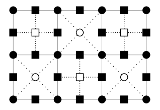
Figure 1: Filled circles and boxes respectively indicate the sites of $\Lambda_{1}$ and $\Lambda_{2}$. Open circles and boxes respectively indicate the sites of $\Omega_{2}$ and $\Omega_{1}$.

For each $x,y\in\Lambda$ and $u\in\Omega$, we set

$$t_{x,y}=\begin{cases}t\ \ &|x-y|=\frac{1}{2}\\ 0\ \ &\text{otherwise},\end{cases}\quad\quad J_{x,u}=\begin{cases}J\ \ &u\in\Omega_{1},|x-u|=\frac{1}{2}\text{\ or\ }u\in\Omega_{2},|x-u|=\frac{1}{\sqrt{2}}\\ 0\ \ &\text{otherwise},\end{cases}$$ (1.29)

where $t\neq 0$. The conditions (C.1)–(C.4) are satisfied. In this example, we simply assume (C.5). First, let us consider the case where $J>0$. Then (C.6) is satisfied. Because $|\Lambda_{2}|=2|\Lambda_{1}|$ and $|\Omega_{1}|=|\Omega_{2}|=|\Lambda_{1}|/2$, the ground state has total spin $S=|\Lambda_{1}|/2=N/8$. Similarly, if $J<0$, then (C.7) is fulfilled and $S=|\Lambda_{1}|/2=N/8$.

Example 3

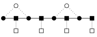
Figure 2: Filled circles and boxes respectively indicate the sites of $\Lambda_{1}$ and $\Lambda_{2}$. Open circles and boxes respectively indicate the sites of $\Omega_{2}$ and $\Omega_{1}$.

In this example, let us consider a chain given by Figure 2. We set

$$t_{x,y}=\begin{cases}t\ \ &|x-y|=\frac{1}{2}\\ 0\ \ &\text{otherwise},\end{cases}\quad\quad J_{x,u}=\begin{cases}J\ \ &u\in\Omega_{1},|x-u|=\frac{1}{2}\text{\ or\ }u\in\Omega_{2},|x-u|=\frac{1}{\sqrt{2}}\\ 0\ \ &\text{otherwise},\end{cases}$$ (1.30)

where $t\neq 0$. With regard to $g_{x,y}$, we simply assume (C.5). Then we readily confirm that $|\Lambda_{1}|=|\Lambda_{2}|=|\Lambda|/2$ and $|\Omega_{1}|=|\Lambda|/2,|\Omega_{2}|=|\Lambda|/4$. Hence, if $J\neq 0$, then the ground state has total spin $S=|\Lambda|/8=N/14$, i.e., the value of $S$ is independent of the sign of $J$.

1.4 Organization

The organization of the present paper is as follows: In Section 2, we present the basics of order preserving operator inequalities. These inequalities are essential to express the idea of the spin reflection positivity, mathematically. Section 3 is devoted to the proof of the uniqueness of the ground state. In Section 4, we give the expression for the total spin of the ground state. In Section 5, we summarize this work and provide discussions. The appendices contain some auxiliary technical statements that are of independent interest.

2 Hilbert cones and their associated operator inequalities

2.1 Basic definitions

In this section, we will briefly review fundamental properties of Hilbert cones and their associated operator inequalities as a preliminary.

Let $\mathcal{X}$ be a complex Hilbert space. We denote by $\mathscr{B}(\mathcal{X})$ the Banach space of all bounded operators on $\mathcal{X}$.

Definition 2.1.

A Hilbert cone, $\mathcal{C}$ in $\mathcal{X}$, is a closed convex cone obeying

• $\langle u,v\rangle\geq 0$ for all $u,v\in\mathcal{C}$;

• for all $w\in\mathcal{X}$, there exist $u,u^{\prime},v,v^{\prime}\in\mathcal{C}$ such that $w=u-v+i(u^{\prime}-v^{\prime})$ and $\langle u,v\rangle=\langle u^{\prime},v^{\prime}\rangle=0.$

A vector $u\in\mathcal{C}$ is said to be positive w.r.t. $\mathcal{C}$. We write this as $u\geq 0$ w.r.t. $\mathcal{C}$. A vector $v\in\mathcal{X}$ is called strictly positive w.r.t. $\mathcal{C}$, whenever $\langle v,u\rangle>0$ for all $u\in\mathcal{C}\setminus\{0\}$. We write this as $v>0$ w.r.t. $\mathcal{C}$.

The following operator inequalities will play a major role in the present paper.

Definition 2.2.

Let $A\in\mathscr{B}(\mathcal{X})$.

• $A$ is positivity preserving if $A\mathcal{C}\subseteq\mathcal{C}$. We write this as $A\unrhd 0\ \text{w.r.t.}\ \mathcal{C}$.

• $A$ is positivity improving if, for all $u\in\mathcal{C}\setminus\{0\},\ Au>0\ \text{w.r.t.}\ \mathcal{C}$. We write this as $A\rhd 0\ \text{w.r.t.}\ \mathcal{C}$.

Remark that the notations of the operator inequalities are borrowed from [13].

We readily confirm the following lemma:

Lemma 2.3.

Let $A,B\in\mathscr{B}(\mathcal{X})$. Suppose that $A,B\unrhd 0\ \text{w.r.t.}\ \mathcal{C}$. We have the following:

• If $a,b\geq 0$, then $aA+bB\unrhd 0\ \text{w.r.t.}\ \mathcal{C}$;

• $AB\unrhd 0\ \text{w.r.t.}\ \mathcal{C}$.

Proof.

For proof, see, e.g., [13, 15]. ∎

Let $\mathcal{X}_{\mathbb{R}}$ be the real subspace of $\mathcal{X}$ generated by $\mathcal{C}$. From Definition 2.1, for all $x\in\mathcal{X}_{\mathbb{R}}$, there exist $x_{+},x_{-}\in\mathcal{C}$ such that $x=x_{+}-x_{-}$ and $\langle x_{+},x_{-}\rangle=0$. If $A\in\mathscr{B}(\mathcal{X})$ satisfies $A\mathcal{X}_{\mathbb{R}}\subseteq\mathcal{X}_{\mathbb{R}}$, then we say that $A$ preserves the reality w.r.t. $\mathcal{C}$.

Definition 2.4.

Let $A,B\in\mathscr{B}(\mathcal{X})$ be reality preserving w.r.t. $\mathcal{C}$. If $A-B\unrhd 0$, then we write this as $A\unrhd B\ \text{w.r.t.}\ \mathcal{C}$.

Below, we provide two fundamental lemmas of the operator inequalities for later use.

Lemma 2.5.

Let $A,B,C,D\in\mathscr{B}(\mathcal{X})$. Suppose $A\unrhd B\unrhd 0\ \text{w.r.t.}\ \mathcal{C}$ and $C\unrhd D\unrhd 0\ \text{w.r.t.}\ \mathcal{C}$. Then we have $AC\unrhd BD\unrhd 0\ \text{w.r.t.}\ \mathcal{C}$

Proof.

For proof, see, e.g., [13, 15]. ∎

Lemma 2.6.

Let $A,B$ be self-adjoint operators on $\mathcal{X}$. Assume that $A$ is bounded from below and that $B\in\mathscr{B}(\mathcal{X})$. Furthermore, suppose that $e^{-tA}\unrhd 0\ \text{w.r.t.}\ \mathcal{C}$ for all $t\geq 0$ and $B\unrhd 0\ \text{w.r.t.}\ \mathcal{C}$. Then we have $e^{-t(A-B)}\unrhd e^{-tA}\ \text{w.r.t.}\ \mathcal{C}$ for all $t\geq 0$.

Proof.

Because $B\unrhd 0\ \text{w.r.t.}\ \mathcal{C}$, we have $e^{tB}=\sum_{n=0}^{\infty}\frac{t^{n}}{n!}B^{n}\unrhd 1\ \text{w.r.t.}\ \mathcal{C}$ for all $t\geq 0$. By the Trotter product formula [28, Theorem S. 20], for all $t\geq 0$, we obtain

$$e^{-t(A-B)}=\lim_{n\to\infty}\left(e^{-\frac{t}{n}A}e^{\frac{t}{n}B}\right)^{n}\unrhd e^{-tA}\ \text{w.r.t.}\ \mathcal{C}.$$ (2.1)

∎

Definition 2.7.

Let $A$ be a self-adjoint operator on $\mathcal{X}$, bounded from below. The semigroup $\{e^{-tA}\}_{t\geq 0}$ is said to be ergodic w.r.t. $\mathcal{C}$, if the following (i) and (ii) are satisfied:

• $e^{-tA}\unrhd 0$ w.r.t. $\mathcal{C}$ for all $t\geq 0$;

• for each $u,v\in\mathcal{C}\setminus\{0\}$, there is a $t\geq 0$ such that $\langle u,e^{-tA}v\rangle>0$. Note that $t$ could depend on $u$ and $v$.

The following lemma immediately follows from the definitions:

Lemma 2.8.

Let $A$ be a self-adjoint operator on $\mathcal{X}$, bounded from below. If $e^{-tA}\rhd 0$ w.r.t. $\mathcal{C}$ for all $t>0$, then $\{e^{-tA}\}_{t\geq 0}$ is ergodic w.r.t. $\mathcal{C}$.

The basic result here is:

Theorem 2.9 (Perron-Frobenius-Faris).

Let $A$ be a self-adjoint operator, bounded from below. Assume that $E(A)=\inf\mathrm{spec}(A)$ is an eigenvalue of $A$, where $\mathrm{spec}(A)$ indicates the spectrum of $A$. Let $\mathcal{V}$ be the eigenspace corresponding to $E(A)$. If $\{e^{-tA}\}_{t\geq 0}$ is ergodic w.r.t. $\mathcal{C}$, then $\dim\mathcal{V}=1$ and $\mathcal{V}$ is spanned by a strictly positive vector w.r.t. $\mathcal{C}$.

Proof.

See [5].∎

2.2 Operator inequalities in $\mathscr{I}_{2}(\mathcal{X})$

Let $\mathscr{I}_{2}(\mathcal{X})$ be the set of all Hilbert-Schmidt operators on $\mathcal{X}$: $\mathscr{I}_{2}(\mathcal{X})=\{\xi\in\mathscr{B}(\mathcal{X})\,|\,\mathrm{Tr}[\xi^{*}\xi]<\infty\}$. In what follows, we regard $\mathscr{I}_{2}(\mathcal{X})$ as a Hilbert space equipped with the inner product $\langle\xi,\eta\rangle_{2}=\mathrm{Tr}[\xi^{*}\eta],\ \xi,\eta\in\mathscr{I}_{2}(\mathcal{X})$. We often abbreviate the inner product by omitting the subscript $2$ if no confusion arises.

Let $\vartheta$ be an antiunitary operator on $\mathcal{X}$. We define the map $\Psi_{\vartheta}:\mathcal{X}\otimes\mathcal{X}\longrightarrow\mathscr{I}_{2}(\mathcal{X})$ by

$$\Psi_{\vartheta}(\phi\otimes\vartheta\psi)=|\phi\rangle\langle\psi|,\quad\phi,\psi\in\mathcal{X}.$$ (2.2)

Since $\Psi_{\vartheta}$ is a unitary operator, we can identify $\mathcal{X}\otimes\mathcal{X}$ with $\mathscr{I}_{2}(\mathcal{X})$, naturally. We write this identification as

$$\mathcal{X}\otimes\mathcal{X}\underset{\Psi_{\vartheta}}{=}\mathscr{I}_{2}(\mathcal{X}).$$ (2.3)

Occasionally, we abbreviate (2.3) by omitting the subscript $\Psi_{\vartheta}$ if no confusion arises.

Given $A\in\mathscr{B}(\mathcal{X})$, we define the left multiplication operator, $\mathcal{L}(A)$, and the right multiplication operator, $\mathcal{R}(A)$, as follows:

$$\mathcal{L}(A)\xi=A\xi,\ \ \mathcal{R}(A)\xi=\xi A,\ \ \xi\in\mathscr{I}_{2}(\mathcal{X}).$$ (2.4)

Trivially, $\mathcal{L}(A)$ and $\mathcal{R}(A)$ are bounded operators on $\mathscr{I}_{2}(\mathcal{X})$. In addition, we readily confirm that

$$\mathcal{L}(A)\mathcal{L}(B)=\mathcal{L}(AB),\ \ \ \mathcal{R}(A)\mathcal{R}(B)=\mathcal{R}(BA).$$ (2.5)

Under the identification (2.3), we have

$$A\otimes 1=\mathcal{L}(A),\ \ \ 1\otimes A=\mathcal{R}(\vartheta A^{*}\vartheta).$$ (2.6)

Let

$$\mathscr{I}_{2,+}(\mathcal{X})=\{\xi\in\mathscr{I}_{2}(\mathcal{X})\,|\,\xi\geq 0\},$$ (2.7)

where the inequality in the right hand side of (2.7) indicates the standard operator inequality. It is well-known that $\mathscr{I}_{2,+}(\mathcal{X})$ is a Hilbert cone in $\mathscr{I}_{2}(\mathcal{X})$, see, e.g., [15, Proposition 2.5]. Using this fact, we can introduce a Hilbert cone in $\mathcal{X}\otimes\mathcal{X}$ by $\mathcal{C}=\Psi_{\vartheta}^{-1}(\mathscr{I}_{2,+}(\mathcal{X}))$. Taking the identification (2.3) into account, we have the following identification:

$$\mathcal{C}=\mathscr{I}_{2,+}(\mathcal{X}).$$ (2.8)

Proposition 2.10.

Let $A\in\mathscr{B}(\mathcal{X})$. Then we have $\mathcal{L}(A)\mathcal{R}(A^{*})\unrhd 0\ \text{w.r.t.}\ \mathscr{I}_{2,+}(\mathcal{X})$. Hence, under the identification (2.3), we have $A\otimes\vartheta A\vartheta\unrhd 0$ w.r.t. $\mathcal{C}$.

Proof.

Take $\xi,\nu\in\mathscr{I}_{2,+}(\mathcal{X})$, arbitrarily. Then there exist sequences of positive numbers, $\{\xi_{n}\}_{n}$ and $\{\nu_{n}\}_{n}$, and complete orthonormal systems(CONSs) $\{x_{n}\}_{n}$ and $\{y_{n}\}_{n}$ in $\mathcal{X}$ such that $\xi=\sum_{n}\xi_{n}|x_{n}\rangle\langle x_{n}|$ and $\nu=\sum_{n}\nu_{n}|y_{n}\rangle\langle y_{n}|$ hold. Because

$$\mathcal{L}(A)\mathcal{R}(A^{*})\nu=\sum_{n}\nu_{n}|Ay_{n}\rangle\langle Ay_{n}|,$$ (2.9)

we have

$$\langle\xi,\mathcal{L}(A)\mathcal{R}(A^{*})\nu\rangle =\sum_{m,n}\xi_{m}\nu_{n}|\langle x_{m},Ay_{n}\rangle|^{2}\geq 0.$$ (2.10)

Hence, we have $\mathcal{L}(A)\mathcal{R}(A^{*})\unrhd 0\ \text{w.r.t.}\ \mathscr{I}_{2,+}(\mathcal{X})$.∎

3 The uniqueness of ground states

3.1 The main result in Section 3

The goal of this section is to prove the first part of Theorem 1.2, that is,

Theorem 3.1.

Assume (C). Suppose that $U_{{\rm eff}}$ is positive semi-definite. Then we obtain the following (i) and (ii):

• The ground state of $H$ is unique.

• We denote by $\psi$ the ground state of $H$. Then $\psi$ satisfies the following:

  $$\gamma_{x}\gamma_{y}\langle\psi,s_{x}^{+}s_{y}^{-}\psi\rangle>0,\ \ \ \gamma_{u}\gamma_{v}\mathrm{sgn}J_{x,u}\mathrm{sgn}J_{y,v}\langle\psi,S_{u}^{+}S_{v}^{-}\psi\rangle>0$$ (3.1)

  for every $x,y\in\Lambda$ and $u,v\in\Omega$.

The proof of Theorem 3.1 will be provided in Subsection 3.6. Our basic strategy for proving Theorem 3.1 is to make use of Theorem 2.9. To realize the strategy, we employ the method of order preserving operator inequalities presented in Section 2.

3.2 Preliminaries

3.2.1 Useful identifications

Let $X=(x_{1},\dots,x_{n})\in\Lambda^{n}$, where $x_{1},\dots,x_{n}$ are mutually different. For such an $X$, let us define a vector in $\bigwedge^{n}\ell^{2}(\Lambda)$ by

$$e_{X}^{c}=\delta_{x_{1}}\wedge\cdots\wedge\delta_{x_{n}},$$ (3.2)

where $\delta_{x}$ is a vector in $\ell^{2}(\Lambda)$ defined by $\delta_{x}(y)=\delta_{x,y}$. Because $\{\delta_{x}\}_{x\in\Lambda}$ is a CONS in $\ell^{2}(\Lambda)$, $\{e_{X}^{c}\}_{X}$ is a CONS of $\mathcal{F}_{F}(\ell^{2}(\Lambda))$. Similarly, for $U=(u_{1},\dots,u_{n})\in\Omega^{n}$, let

$$e^{f}_{U}=\delta_{u_{1}}\wedge\cdots\wedge\delta_{u_{n}}.$$ (3.3)

Then $\{e^{f}_{U}\}_{U}$ is a CONS of $\mathcal{F}_{\rm F}(\ell^{2}(\Omega))$. Trivially, $\{e^{c}_{X_{\uparrow}}\otimes e^{c}_{X_{\downarrow}}\}_{X_{\uparrow},X_{\downarrow}}$ and $\{e^{f}_{U_{\uparrow}}\otimes e^{f}_{U_{\downarrow}}\}_{U_{\uparrow},U_{\downarrow}}$ are canonical CONSs in $\mathcal{H}_{\rm c}$ and $\mathcal{H}_{\rm f}$, respectively. Hence, a canonical CONS in $\mathcal{H}_{\rm c}\otimes\mathcal{H}_{\rm f}$ is given by $\{e^{c}_{X_{\uparrow}}\otimes e^{c}_{X_{\downarrow}}\otimes e^{f}_{U_{\uparrow}}\otimes e^{f}_{U_{\downarrow}}\}_{X_{\uparrow},X_{\downarrow},U_{\uparrow},U_{\downarrow}}$.

In what follows, we will freely use the following identification:

$$\mathcal{H}_{\rm c}\otimes\mathcal{H}_{\rm f}=\mathcal{F}\otimes\mathcal{F},$$ (3.4)

where $\mathcal{F}=\mathcal{F}_{\rm F}(\ell^{2}(\Lambda))\otimes\mathcal{F}_{\rm F}(\ell^{2}(\Omega))=\mathcal{F}_{\rm F}(\ell^{2}(\Lambda)\oplus\ell^{2}(\Omega))$. (Here, the identification $\mathcal{F}_{\rm F}(\ell^{2}(\Lambda))\otimes\mathcal{F}_{\rm F}(\ell^{2}(\Omega))=\mathcal{F}_{\rm F}(\ell^{2}(\Lambda)\oplus\ell^{2}(\Omega))$ is due to the footnote including (1.7) in Subsection 1.2.) Note that this identification is implemented by the unitary operator $\tau$ given by

$$\tau e^{c}_{X_{\uparrow}}\otimes e^{c}_{X_{\downarrow}}\otimes e^{f}_{U_{\uparrow}}\otimes e^{f}_{U_{\downarrow}}=e^{c}_{X_{\uparrow}}\otimes e^{f}_{U_{\uparrow}}\otimes e^{c}_{X_{\downarrow}}\otimes e^{f}_{U_{\downarrow}}.$$ (3.5)

Next, we define the antiunitary operator $\vartheta:\mathcal{F}\longrightarrow\mathcal{F}$ by

$$\vartheta\left(\sum_{X,U}c(X,U)e^{c}_{X}\otimes e^{f}_{U}\right)=\sum_{X,U}\overline{c(X,U)}e^{c}_{X}\otimes e^{f}_{U},\ \ c(X,U)\in\mathbb{C}.$$ (3.6)

With this choice of $\vartheta$, we can identify $\mathcal{F}\otimes\mathcal{F}$ with $\mathscr{I}_{2}(\mathcal{F})$ by using (2.3).

To sum, we obtain the following:

$$\mathcal{H}_{\rm c}\otimes\mathcal{H}_{\rm f}\underset{\tau}{=}\mathcal{F}\otimes\mathcal{F}\underset{\Psi_{\vartheta}}{=}\mathscr{I}_{2}(\mathcal{F}).$$ (3.7)

As we will see in the following sections, the above identifications play an important role.

Recall that $N=|\Lambda|+|\Omega|$. Let $\mathcal{F}_{N}=\bigwedge^{N/2}\left(\ell^{2}(\Lambda)\oplus\ell^{2}(\Omega)\right)$. Then, due to the footnote including (1.7) in Subsection 1.2, $\mathcal{L}_{N}$ defined by (1.17) can be expressed as

$$\mathcal{L}_{N}=\mathcal{F}_{N}\otimes\mathcal{F}_{N}.$$ (3.8)

Moreover, taking (3.7) into account, we have the following identification:

$$\mathcal{L}_{N}=\mathscr{I}_{2}(\mathcal{F}_{N}).$$ (3.9)

Let $\mathsf{c}_{x}$ and $\mathsf{f}_{u}$ be the annihilation operators on $\mathcal{F}$ such that $\{\mathsf{c}_{x},\mathsf{c}_{y}^{*}\}=\delta_{x,y}\ (x,y\in\Lambda)$, $\{\mathsf{f}_{u},\mathsf{f}_{v}^{*}\}=\delta_{u,v}\ (u,v\in\Omega)$ and $\{\mathsf{c}_{x},{\sf f}_{u}\}=0=\{{\sf c}_{x},{\sf f}_{u}^{*}\}\ (x\in\Lambda,u\in\Omega)$. Note that $c_{x\sigma}$ and $f_{u\sigma}$ can be rewritten as

$$c_{x\uparrow}=\mathsf{c}_{x}\otimes 1,\ \ f_{u\uparrow}=\mathsf{f}_{u}\otimes 1,\ \ c_{x\downarrow}=(-1)^{\mathsf{N}}\otimes\mathsf{c}_{x},\ \ f_{u\downarrow}=(-1)^{\mathsf{N}}\otimes\mathsf{f}_{u},$$ (3.10)

where $\mathsf{N}$ is the number operator given by $\mathsf{N}=\sum_{x\in\Lambda}\mathsf{n}_{x}^{c}+\sum_{u\in\Omega}\mathsf{n}_{u}^{f}$ with $\mathsf{n}_{x}^{c}=\mathsf{c}_{x}^{*}\mathsf{c}_{x}$ and $\mathsf{n}_{u}^{f}=\mathsf{f}_{u}^{*}\mathsf{f}_{u}$. Using (2.6), we obtain the fundamental identifications:

$$c_{x\uparrow}=\mathcal{L}(\mathsf{c}_{x}),\ \ c_{x\downarrow}=\mathcal{L}\big{(}(-1)^{\mathsf{N}}\big{)}\mathcal{R}(\mathsf{c}_{x}^{*}),\ \ f_{u\uparrow}=\mathcal{L}(\mathsf{f}_{u}),\ \ f_{u\downarrow}=\mathcal{L}\big{(}(-1)^{\mathsf{N}}\big{)}\mathcal{R}(\mathsf{f}_{u}^{*}).$$ (3.11)

From these formulas, we can freely produce useful formulas. For instance,

$$n_{x\uparrow}^{c}=\mathcal{L}(\mathsf{n}_{x}^{c}),\ \ n^{c}_{x\downarrow}=\mathcal{R}(\mathsf{n}_{x}^{c}),\ \ n^{f}_{u\uparrow}=\mathcal{L}(\mathsf{n}_{u}^{f}),\ \ n^{f}_{u\downarrow}=\mathcal{R}(\mathsf{n}_{u}^{f}).$$ (3.12)

3.2.2 Basic Hilbert cones

As Theorem 2.9 suggests, Hilbert cones are important in order to prove the uniqueness of the ground state of $H$. The aim of this subsection is to introduce basic Hilbert cones which are essential to the proof of Theorem 3.1.

We define the Hilbert cone $\mathcal{P}$ in $\mathcal{H}_{\rm ph}$ by

$$\mathcal{P}=L_{+}^{2}(\mathbb{R}^{|\Lambda|}),$$ (3.13)

where $L_{+}^{2}(\mathbb{R}^{|\Lambda|})=\{f\in L^{2}(\mathbb{R}^{|\Lambda|})\,|\,f({\bm{q}})\geq 0\text{ a.e. ${\bm{q}}$}\}.$ Note that the number operator $N_{\rm p}$ can be identified with the Hamiltonian of the harmonic oscillators:

$$N_{\rm p}=\sum_{x\in\Lambda}\frac{1}{2}\big{(}-\Delta_{q_{x}}+q_{x}^{2}-1\big{)},$$ (3.14)

where $\Delta_{q_{x}}$ is the Laplacian. As is well-known, it holds that

$$e^{-\beta\omega_{0}N_{\rm p}}\rhd 0$$ (3.15)

w.r.t. $\mathcal{P}$ for all $\beta>0$. This property will be repeatedly used in the following sections.

Using the identification (3.8), we introduce a Hilbert cone, $\mathcal{L}_{N,+}$, of $\mathcal{L}_{N}$ by

$$\mathcal{L}_{N,+}=\mathscr{I}_{2}(\mathcal{F}_{N})_{+}=\{\psi\in\mathcal{L}_{N}\,|\,\Psi_{\vartheta}(\psi)\geq 0\},$$ (3.16)

where the inequality in (3.16) means the standard operator inequality.

Define

$$Q_{0} =\prod_{u\in\Omega}\left[n_{u\uparrow}^{f}n_{u\downarrow}^{f}+\big{(}1-n_{u\uparrow}^{f}\big{)}\big{(}1-n_{u\downarrow}^{f}\big{)}\right].$$ (3.17)

Then $Q_{0}$ is an orthogonal projection on $\mathcal{L}_{N}=\mathscr{I}_{2}(\mathcal{F}_{N})$.

Lemma 3.2.

$Q_{0}\mathcal{L}_{N,+}$ is a Hilbert cone in $Q_{0}\mathcal{L}_{N}$.

Proof.

Using (3.12), we find

$$n_{u\uparrow}^{f}n_{u\downarrow}^{f} =\mathcal{L}(\mathsf{n}_{u}^{f})\mathcal{R}(\mathsf{n}_{u}^{f}),\ \ \big{(}1-n_{u\uparrow}^{f}\big{)}\big{(}1-n_{u\downarrow}^{f}\big{)}=\mathcal{L}(1-\mathsf{n}_{u}^{f})\mathcal{R}(1-\mathsf{n}_{u}^{f}).$$ (3.18)

Thus, from Proposition 2.10, $n_{u\uparrow}^{f}n_{u\downarrow}^{f}\unrhd 0$ and $\big{(}1-n_{u\uparrow}^{f}\big{)}\big{(}1-n_{u\downarrow}^{f}\big{)}\unrhd 0\ \text{w.r.t.}\ \mathcal{L}_{N,+}$ hold, which imply $Q_{0}\unrhd 0\ \text{w.r.t.}\ \mathcal{L}_{N,+}$. Since $\mathcal{L}_{N,+}$ is a Hilbert cone in $\mathcal{L}_{N}$ and $Q_{0}\unrhd 0\ \text{w.r.t.}\ \mathcal{L}_{N,+}$, we readily confirm that $Q_{0}\mathcal{L}_{N,+}$ is a Hilbert cone in $Q_{0}\mathcal{L}_{N}$.∎

Next, we define

$$\mathcal{Q} =\overline{\mathrm{coni}}\{\psi\otimes f\in Q_{0}\mathcal{L}_{N}\otimes\mathcal{H}_{\rm ph}\,|\,\psi\in Q_{0}\mathcal{L}_{N,+},f\in\mathcal{P}\},$$ (3.19)

where $\overline{\mathrm{coni}}\,X$ is the closure of the conical hull of $X$. The following proposition is crucial in the present paper.

Proposition 3.3.

$\mathcal{Q}$ is a Hilbert cone in $Q_{0}\mathcal{L}_{N}\otimes\mathcal{H}_{\rm ph}$.

Proof.

See Appendix D.∎

The following basic lemma is often useful.

Lemma 3.4.

Let $A$ be a bounded operator on $Q_{0}\mathcal{L}_{N}\otimes\mathcal{H}_{\rm ph}$. Let $B$ be a self-adjoint operator on $Q_{0}\mathcal{L}_{N}\otimes\mathcal{H}_{\rm ph}$, bounded from below. Assume that $e^{-tB}\unrhd 0\ \text{w.r.t.}\ \mathcal{Q}$ for any $t\geq 0$. We have the following:

• If $A$ satisfies $\langle\phi\otimes f,A\psi\otimes g\rangle\geq 0$ for all $\phi,\psi\in Q_{0}\mathcal{L}_{N,+}$ and $f,g\in\mathcal{P}$, then we have $A\unrhd 0\ \text{w.r.t.}\ \mathcal{Q}$.

• If $A$ satisfies $\langle\phi\otimes f,A\psi\otimes g\rangle>0$ for all $\phi,\psi\in Q_{0}\mathcal{L}_{N,+}\setminus\{0\}$ and $f,g\in\mathcal{P}\setminus\{0\}$, then we have $A\rhd 0\ \text{w.r.t.}\ \mathcal{Q}$.

• Assume that $e^{-tB}\unrhd 0$ w.r.t. $\mathcal{Q}$ for all $t\geq 0$. In addition, assume that, for all $\phi,\psi\in Q_{0}\mathcal{L}_{N,+}\setminus\{0\}$ and $f,g\in\mathcal{P}\setminus\{0\}$, there exists a $t\geq 0$ such that $\langle\phi\otimes f,e^{-tB}\psi\otimes g\rangle>0$. Then $\{e^{-tB}\}_{t\geq 0}$ is ergodic w.r.t. $\mathcal{Q}$.

Proof.

(i) From the definition of $\mathcal{Q}$, for any $u,v\in\mathcal{Q}$, there exist $\psi_{n}\otimes f_{n}$ and $\phi_{n}\otimes g_{n}\in\mathcal{Q}$ satisfying

$$u=\sum_{n\geq 1}\psi_{n}\otimes f_{n},\ \ v=\sum_{n\geq 1}\phi_{n}\otimes g_{n}.$$ (3.20)

Using these expressions, we obtain $\langle u,Av\rangle=\sum_{m,n\geq 1}\langle\psi_{m}\otimes f_{m},A\phi_{n}\otimes g_{n}\rangle\geq 0,$ which implies that $A\unrhd 0\ \text{w.r.t.}\ \mathcal{Q}$.

(ii) Let $u,v\in\mathcal{Q}\setminus\{0\}$. Then $u$ and $v$ can be expressed as (3.20). Because $u$ and $v$ are non-zero, there exist $k,l\in\mathbb{N}$ such that $\psi_{k}\otimes f_{k}\neq 0$ and $\phi_{l}\otimes g_{l}\neq 0$. Hence, we obtain $\langle u,Av\rangle=\sum_{m,n\geq 1}\langle\psi_{m}\otimes f_{m},A\phi_{n}\otimes g_{n}\rangle\geq\langle\psi_{k}\otimes f_{k},A\phi_{l}\otimes g_{l}\rangle>0,$ which implies that $A\rhd 0\ \text{w.r.t.}\ \mathcal{Q}$.

(iii) Let $u,v\in\mathcal{Q}\setminus\{0\}$. We continue to employ the expressions (3.20). Because $u$ and $v$ are non-zero, there exist $k,l\in\mathbb{N}$ such that $\psi_{k}\otimes f_{k}\neq 0$ and $\phi_{l}\otimes g_{l}\neq 0$. By the assumption, there exists a $t\geq 0$ such that $\langle\psi_{k}\otimes f_{k},e^{-tB}\phi_{l}\otimes g_{l}\rangle>0$. Since $e^{-tB}\unrhd 0\ \text{w.r.t.}\ \mathcal{Q}$, it holds that $\langle u,e^{-tB}v\rangle\geq\langle\psi_{k}\otimes f_{k},e^{-tB}\phi_{l}\otimes g_{l}\rangle>0$. Hence, $\{e^{-tB}\}_{t\geq 0}$ is ergodic w.r.t. $\mathcal{Q}$.∎

In what follows, we use the following identification:

$$Q_{0}\mathcal{L}_{N}\otimes\mathcal{H}_{\rm ph}=\int^{\oplus}_{\mathbb{R}^{|\Lambda|}}Q_{0}\mathcal{L}_{N}d{\bm{q}},$$ (3.21)

where the right hand side of (3.21) is the constant fiber direct integral [27, Section XIII.16].

Lemma 3.5.

Let $A\in\mathscr{B}(Q_{0}\mathcal{L}_{N}\otimes\mathcal{H}_{\rm ph})$ be a decomposable operator:

$$A=\int_{\mathbb{R}^{|\Lambda|}}^{\oplus}A(\bm{q})\,d\bm{q}.$$ (3.22)

If $A(\bm{q})\unrhd 0\ \text{w.r.t.}\ Q_{0}\mathcal{L}_{N,+}$ for a.e. ${\bm{q}}$, then we have $A\unrhd 0\ \text{w.r.t.}\ \mathcal{Q}$.

Proof.

Take $\phi,\psi\in Q_{0}\mathcal{L}_{N,+}$ and $f,g\in\mathcal{P}$, arbitrarily. Since $A(\bm{q})\unrhd 0\ \text{w.r.t.}\ Q_{0}\mathcal{L}_{N,+}$ and $f({\bm{q}}),g({\bm{q}})\geq 0$ a.e., we have

$$\left\langle\phi\otimes f,A\psi\otimes g\right\rangle=\int_{\mathbb{R}^{|\Lambda|}}f(\bm{q})g(\bm{q})\left\langle\phi,A(\bm{q})\psi\right\rangle\,d\bm{q}\geq 0.$$ (3.23)

By Lemma 3.4, we conclude that $A\unrhd 0\ \text{w.r.t.}\ \mathcal{Q}$. ∎

Lemma 3.6.

Let $A\in\mathscr{B}(\mathcal{L}_{N})$. Assume the following:

• $A$ commutes with $Q_{0}$.

• $A\unrhd 0$ w.r.t. $\mathcal{L}_{N,+}$ where $\mathcal{L}_{N,+}$ is given by (3.16).

Then we have $A\restriction Q_{0}\mathcal{L}_{N}\unrhd 0\ \text{w.r.t.}\ Q_{0}\mathcal{L}_{N,+}$, where $A\restriction Q_{0}\mathcal{L}_{N}$ is the restriction of $A$ to $Q_{0}\mathcal{L}_{N}$.

Proof.

Since $Q_{0}\unrhd 0\ \text{w.r.t.}\ \mathcal{L}_{N,+}$, we see $Q_{0}AQ_{0}\unrhd 0\ \text{w.r.t.}\ \mathcal{L}_{N,+}$. Hence, for any $\phi,\psi\in\mathcal{L}_{N,+}$, $\langle\phi,Q_{0}AQ_{0}\psi\rangle=\langle Q_{0}\phi,AQ_{0}\psi\rangle\geq 0$ holds. Thus, we have $A\unrhd 0\ \text{w.r.t.}\ Q_{0}\mathcal{L}_{N,+}$.∎

Lemma 3.7.

Let $A,B\in\mathscr{B}(\mathcal{F}_{N})$. Assume that $A\otimes 1+1\otimes\vartheta A\vartheta$ and $B\otimes\vartheta B\vartheta$ commute with $Q_{0}$. Then we have

$$\exp\{(A\otimes 1+1\otimes\vartheta A\vartheta)\restriction Q_{0}\mathcal{L}_{N}\} \unrhd 0\ \text{w.r.t.}\ Q_{0}\mathcal{L}_{N,+},$$ (3.24)

$$B\otimes\vartheta B\vartheta\restriction Q_{0}\mathcal{L}_{N} \unrhd 0\ \text{w.r.t.}\ Q_{0}\mathcal{L}_{N,+}.$$ (3.25)

Proof.

Using Proposition 2.10, we have

$$e^{A\otimes 1+1\otimes\vartheta A\vartheta}=e^{A}\otimes\vartheta e^{A}\vartheta\unrhd 0\ \text{w.r.t.}\ \mathcal{L}_{N,+},$$ (3.26)

$$B\otimes\vartheta B\vartheta\unrhd 0\ \text{w.r.t.}\ \mathcal{L}_{N,+}.$$ (3.27)

Thus, applying Lemma 3.6, we obtain the desired results. ∎

Lemma 3.8.

Let $A\in\mathscr{B}(Q_{0}\mathcal{L}_{N})$. Assume that $A\unrhd 0\ \text{w.r.t.}\ Q_{0}\mathcal{L}_{N,+}$. Then we have $A\otimes 1\unrhd 0\ \text{w.r.t.}\ \mathcal{Q}$,

Proof.

For any $\phi,\psi\in Q_{0}\mathcal{L}_{N,+}$ and $f,g\in\mathcal{P}$, we observe that

$$\langle\phi\otimes f,A\otimes 1\psi\otimes g\rangle=\langle\phi,A\psi\rangle\langle f,g\rangle\geq 0.$$ (3.28)

Hence, by applying Lemma 3.4, we conclude that $A\otimes 1\unrhd 0\ \text{w.r.t.}\ \mathcal{Q}$.∎

Lemma 3.9.

Let $A\in\mathscr{B}(Q_{0}\mathcal{L}_{N}\otimes\mathcal{H}_{\rm ph})$. Assume $A\unrhd 0\ \text{w.r.t.}\ \mathcal{Q}$. Then we have $e^{A}\unrhd 0\ \text{w.r.t.}\ \mathcal{Q}$.

Proof.

By the assumption, we obtain $A^{n}\unrhd 0\ \text{w.r.t.}\ \mathcal{Q},n=0,1,\ldots$. Thus, we find $e^{A}=\sum_{n=0}^{\infty}\frac{1}{n!}A^{n}\unrhd 0\ \text{w.r.t.}\ \mathcal{Q}.$ ∎

3.3 Basic transformations

In order to properly apply the theory given in Section 2, we introduce a useful transformation; the definition of $\mathcal{U}$, i.e., (3.50) and Corollary 3.13 are fundamental results in this subsection.

We begin with the following lemma.

Lemma 3.10.

There exists a unitary operator $U$ on $\mathcal{L}_{N}$ satisfying

$$U^{*}c_{x\uparrow}U=c_{x\uparrow},\quad U^{*}f_{u\uparrow}U=f_{u\uparrow},\quad U^{*}c_{x\downarrow}U=\gamma_{x}c_{x\downarrow}^{*},\quad U^{*}f_{u\downarrow}U=\gamma_{u}\mathrm{sgn}J_{x,u}f_{u\downarrow}^{*},$$ (3.29)

where

$$\gamma_{z}=\begin{cases}-1\ \ &(z\in\Lambda_{1}\ or\ z\in\Omega_{1})\\ 1\ \ &(z\in\Lambda_{2}\ or\ z\in\Omega_{2}),\end{cases}$$ (3.30)

and $\mathrm{sgn}J_{x,u}$ is determined by the assumption (C.2).

Proof.

Let $U_{1}$ be the unitary operator on $\mathcal{H}_{\rm c}$ such that

$$U_{1}^{*}c_{x\uparrow}U_{1}=c_{x\uparrow},\quad U_{1}^{*}c_{x\downarrow}U_{1}=\gamma_{x}c_{x\downarrow}^{*}.$$ (3.31)

Note that $U_{1}$ is the standard hole-particle transformation on $\mathcal{H}_{\rm c}$.

By (C.2), for any $u\in\Omega$, there exists an $x_{u}\in\Lambda$ satisfying $J_{x_{u},u}\neq 0$. Note that $\mathrm{sgn}J_{x_{u},u}$ is independent of the choice of $x_{u}$. Let $U_{2}$ be the unitary operator on $\mathcal{H}_{\rm f}$ such that

$$U_{2}^{*}f_{u\uparrow}U_{2}=f_{u\uparrow},\quad U_{2}^{*}f_{u\downarrow}U_{2}=\gamma_{u}\mathrm{sgn}J_{x_{u},u}f_{u\downarrow}^{*}.$$ (3.32)

Choosing $U=U_{1}\otimes U_{2}$, we readily confirm that $U$ satisfies the desired properties in (3.30). ∎

For each $x\in\Lambda$, define self-adjoint operators, $p_{x}$ and $q_{x}$, by

$$p_{x}=\frac{i}{\sqrt{2}}(\overline{b_{x}^{*}-b_{x}}),\ \ \ q_{x}=\frac{1}{\sqrt{2}}(\overline{b_{x}^{*}+b_{x}}),$$ (3.33)

where $\overline{A}$ is the closure of $A$. As is well-known, these operators satisfy the standard commutation relation: $[q_{x},p_{y}]=i\delta_{x,y}$.

Lemma 3.11.

We set

$$L_{c}=-i\frac{\sqrt{2}}{\omega_{0}}\sum_{x,y\in\Lambda}g_{x,y}n_{x}^{c}p_{y}.$$ (3.34)

The unitary operator $e^{L_{c}}$ is called the Lang-Firsov transformation which was first introduced in [9]. Let $N_{\rm p}$ be the phonon number operator: $N_{\rm p}=\sum_{x\in\Lambda}b_{x}^{*}b_{x}$. Then

$$e^{i\frac{\pi}{2}N_{\rm p}}e^{L_{c}}He^{-L_{c}}e^{-i\frac{\pi}{2}N_{\rm p}}$$

$$=-T_{\uparrow}^{+}-T_{\downarrow}^{+}+\sum_{x\in\Lambda,u\in\Omega}J_{x,u}{\bm{s}}_{x}\cdot{\bm{S}}_{u}+\mathbb{U}+\omega_{0}N_{\rm p}-\omega_{0}^{-1}g^{2}|\Lambda|$$ (3.35)

holds, where $T_{\sigma}^{\pm},\mathbb{U}$ and $g$ are defined respectively by

• $\displaystyle T_{\sigma}^{\pm}=\sum_{x,y\in\Lambda}t_{x,y}c_{x\sigma}^{*}c_{y\sigma}\exp\left(\pm i\Phi_{x,y}\right)$ with $\Phi_{x,y}=\frac{\sqrt{2}}{\omega_{0}}\sum_{z\in\Lambda}(g_{xz}-g_{yz})q_{z};$

• $\displaystyle\mathbb{U}=\sum_{x,y\in\Lambda}U_{\mathrm{eff},xy}(n_{x}^{c}-1)(n_{y}^{c}-1)$ with $U_{{\rm eff},xy}$ given by (1.19);

• $g=\sum_{x\in\Lambda}g_{x,y}$. Note that $g$ is independent of $y$ due to (C.5).

Proof.

Let $\mathbb{T}=\displaystyle\sum_{x,y\in\Lambda}\sum_{\sigma=\uparrow,\downarrow}t_{x,y}c_{x\sigma}c_{y\sigma}$. Applying properties of basic operators in Appendix A, we have

$$e^{i\frac{\pi}{2}N_{\rm p}}e^{L_{c}}\mathbb{T}e^{-L_{c}}e^{-i\frac{\pi}{2}N_{\rm p}} =-T_{\uparrow}^{+}-T_{\downarrow}^{+},$$ (3.36)

$$e^{i\frac{\pi}{2}N_{\rm p}}e^{L_{c}}\Bigg{(}\sum_{x\in\Lambda,u\in\Omega}J_{x,u}{\bm{s}}_{x}\cdot{\bm{S}}_{u}\Bigg{)}e^{-L_{c}}e^{-i\frac{\pi}{2}N_{\rm p}} =\sum_{x\in\Lambda,u\in\Omega}J_{x,u}{\bm{s}}_{x}\cdot{\bm{S}}_{u},$$ (3.37)

$$e^{i\frac{\pi}{2}N_{\rm p}}e^{L_{c}}\Bigg{\{}\sum_{x,y\in\Lambda}U_{x,y}(n_{x}^{c}-1)(n_{y}^{c}-1)\Bigg{\}}e^{-L_{c}}e^{-i\frac{\pi}{2}N_{\rm p}} =\sum_{x,y\in\Lambda}U_{x,y}(n_{x}^{c}-1)(n_{y}^{c}-1),$$ (3.38)

$$e^{L_{c}}\Bigg{\{}\sum_{x,y\in\Lambda}g_{x,y}n_{x}^{c}(b_{y}^{*}+b_{y})\Bigg{\}}e^{-L_{c}} =\sum_{x,y\in\Lambda}g_{x,y}n_{x}^{c}(b_{y}^{*}+b_{y})-\frac{2}{\omega_{0}}\sum_{x,y,z\in\Lambda}g_{x,z}g_{y,z}n_{x}^{c}n_{y}^{c},$$ (3.39)

$$e^{L_{c}}N_{\rm p}e^{-L_{c}} =N_{\rm p}-\frac{1}{\omega_{0}}\sum_{x,y\in\Lambda}g_{x,y}n_{x}^{c}(b_{y}^{*}+b_{y})+\omega_{0}^{-2}\sum_{x,y,z\in\Lambda}g_{x,z}g_{y,z}n_{x}^{c}n_{y}^{c}.$$ (3.40)

Combining (3.39) and (3.40), we find

$$e^{i\frac{\pi}{2}N_{\rm p}}e^{L_{c}}\Bigg{\{}\sum_{x,y\in\Lambda}g_{x,y}n_{x}^{c}(b_{y}^{*}+b_{y})+\omega_{0}N_{\rm p}\Bigg{\}}e^{-L_{c}}e^{-i\frac{\pi}{2}N_{\rm p}}$$

$$=\omega_{0}N_{\rm p}-\sum_{x,y\in\Lambda}V_{x,y}n_{x}^{c}n_{y}^{c}$$

$$=\omega_{0}N_{\rm p}-\sum_{x,y\in\Lambda}V_{x,y}(n_{x}^{c}-1)(n_{y}^{c}-1)-\sum_{x,y\in\Lambda}V_{x,y}(n_{x}^{c}+n_{y}^{c})+\sum_{x,y\in\Lambda}V_{x,y}$$

$$=\omega_{0}N_{\rm p}-\sum_{x,y\in\Lambda}V_{x,y}(n_{x}^{c}-1)(n_{y}^{c}-1)-\omega_{0}^{-1}\sum_{x,y,z\in\Lambda}g_{x,z}g_{y,z}(n_{x}^{c}+n_{y}^{c})+\omega_{0}^{-1}\sum_{x,y,z\in\Lambda}g_{x,z}g_{y,z}$$

$$=\omega_{0}N_{\rm p}-\sum_{x,y\in\Lambda}V_{x,y}(n_{x}^{c}-1)(n_{y}^{c}-1)-\omega_{0}^{-1}g\sum_{x,z\in\Lambda}g_{x,z}n_{x}^{c}-\omega_{0}^{-1}g\sum_{y,z\in\Lambda}g_{y,z}n_{y}^{c}+\omega_{0}^{-1}g^{2}|\Lambda|$$

$$=\omega_{0}N_{\rm p}-\sum_{x,y\in\Lambda}V_{x,y}(n_{x}^{c}-1)(n_{y}^{c}-1)-2\omega_{0}^{-1}g^{2}\sum_{x\in\Lambda}n_{x}^{c}+\omega_{0}^{-1}g^{2}|\Lambda|$$

$$=\omega_{0}N_{\rm p}-\sum_{x,y\in\Lambda}V_{x,y}(n_{x}^{c}-1)(n_{y}^{c}-1)-\omega_{0}^{-1}g^{2}|\Lambda|,$$ (3.41)

where $V_{x,y}=\omega_{0}^{-1}\sum_{z\in\Lambda}g_{x,z}g_{y,z}$. Therefore, we finally obtain

$$e^{i\frac{\pi}{2}N_{\rm p}}e^{L_{c}}He^{-L_{c}}e^{-i\frac{\pi}{2}N_{\rm p}}$$

$$=-T_{\uparrow}^{+}-T_{\downarrow}^{+}+\sum_{x\in\Lambda,u\in\Omega}J_{x,u}{\bm{s}}_{x}\cdot{\bm{S}}_{u}+\mathbb{U}+\omega_{0}N_{\rm p}-\omega_{0}^{-1}g^{2}|\Lambda|.$$ (3.42)

∎

Lemma 3.12.

Set

$$H^{\prime}=-T_{\uparrow}^{+}-T_{\downarrow}^{-}+\sum_{x\in\Lambda,u\in\Omega}J_{x,u}{\bm{s}}_{x}\cdot{\bm{S}}_{u}+\mathbb{U}.$$ (3.43)

Then we have

$$U^{*}H^{\prime}U=R-\frac{1}{2}\sum_{x\in\Lambda,u\in\Omega}|J_{x,u}|\left(c_{x\uparrow}^{*}f_{u\uparrow}c_{x\downarrow}^{*}f_{u\downarrow}+f_{u\uparrow}^{*}c_{x\uparrow}f_{u\downarrow}^{*}c_{x\downarrow}\right)-\tilde{\mathbb{U}},$$ (3.44)

where

$$R =-T_{\uparrow}^{+}-T_{\downarrow}^{-}+\frac{1}{4}\sum_{x\in\Lambda,u\in\Omega}J_{x,u}(n_{x}^{c}-1)(n_{u}^{f}-1)+\sum_{x,y\in\Lambda}U_{\mathrm{eff},x,y}(n_{x\uparrow}^{c}n_{y\uparrow}^{c}+n_{x\downarrow}^{c}n_{y\downarrow}^{c}),$$ (3.45)

$$\tilde{\mathbb{U}} =2\sum_{x,y\in\Lambda}U_{\mathrm{eff},x,y}n_{x\uparrow}^{c}n_{y\downarrow}^{c}.$$ (3.46)

Proof.

By using (C.1) and (C.3), we have

$$U^{*}(T_{\uparrow}^{+}+T_{\downarrow}^{+})U =T_{\uparrow}^{+}+\sum_{x,y\in\Lambda}t_{x,y}\gamma_{x}\gamma_{y}c_{x\downarrow}c_{y\downarrow}^{*}\exp(i\Phi_{x,y})$$

$$=T_{\uparrow}^{+}-\sum_{x,y\in\Lambda}t_{x,y}c_{x\downarrow}c_{y\downarrow}^{*}\exp(i\Phi_{x,y})$$

$$=T_{\uparrow}^{+}+\sum_{x,y\in\Lambda}t_{x,y}c_{y\downarrow}^{*}c_{x\downarrow}\exp(-i\Phi_{y,x})$$

$$=T_{\uparrow}^{+}+T_{\downarrow}^{-},$$ (3.47)

$$U^{*}\mathbb{U}U =\sum_{x,y\in\Lambda}U_{\mathrm{eff},x,y}(n_{x\uparrow}^{c}-n_{x\downarrow}^{c})(n_{y\uparrow}^{c}-n_{y\downarrow}^{c})$$

$$=\sum_{x,y\in\Lambda}U_{\mathrm{eff},x,y}(n_{x\uparrow}^{c}n_{y\uparrow}^{c}+n_{x\downarrow}^{c}n_{y\downarrow}^{c})-2\sum_{x,y\in\Lambda}U_{\mathrm{eff},x,y}n_{x\uparrow}^{c}n_{y\downarrow}^{c},$$ (3.48)

and

$$U^{*}\sum_{x\in\Lambda,u\in\Omega}J_{x,u}{\bm{s}}_{x}\cdot{\bm{S}}_{u}U$$

$$=\sum_{x\in\Lambda,u\in\Omega}J_{x,u}U^{*}\Big{(}\frac{1}{2}s_{x}^{+}S_{u}^{-}+\frac{1}{2}s_{x}^{-}S_{u}^{+}+s_{x}^{(3)}S_{u}^{(3)}\Big{)}U$$

$$=\sum_{x\in\Lambda,u\in\Omega}J_{x,u}U^{*}\Big{\{}\frac{1}{2}c_{x\uparrow}^{*}c_{x\downarrow}f_{u\downarrow}^{*}f_{u\uparrow}+\frac{1}{2}c_{x\downarrow}^{*}c_{x\uparrow}f_{u\uparrow}^{*}f_{u\downarrow}+\frac{1}{4}(n_{x\uparrow}^{c}-n_{x\downarrow}^{c})(n_{u\uparrow}^{f}-n_{u\downarrow}^{f})\Big{\}}U$$

$$=-\frac{1}{2}\sum_{x\in\Lambda,u\in\Omega}|J_{x,u}|\left(c_{x\uparrow}^{*}f_{u\uparrow}c_{x\downarrow}^{*}f_{u\downarrow}+f_{u\uparrow}^{*}c_{x\uparrow}f_{u\downarrow}^{*}c_{x\downarrow}\right)+\frac{1}{4}\sum_{x\in\Lambda,u\in\Omega}J_{x,u}(n_{x}^{c}-1)(n_{u}^{f}-1).$$ (3.49)

Combining (3.47) and (3.49), we conclude (3.44). ∎

Define

$$\mathcal{U}=e^{-L_{c}}e^{-i\frac{\pi}{2}N_{\rm p}}U.$$ (3.50)

Note that

$$\mathcal{U}^{*}P_{0}\mathcal{U}=Q_{0}.$$ (3.51)

Hence, $\mathcal{U}^{*}H\mathcal{U}$ acts on $Q_{0}\mathcal{L}_{N}\otimes\mathcal{H}_{\rm ph}$. Applying Lemmas 3.11 and 3.12, we obtain the following:

Corollary 3.13.

Let

$$\mathbb{J}=\frac{1}{2}\sum_{x\in\Lambda,u\in\Omega}|J_{x,u}|\left(c_{x\uparrow}^{*}f_{u\uparrow}c_{x\downarrow}^{*}f_{u\downarrow}+f_{u\uparrow}^{*}c_{x\uparrow}f_{u\downarrow}^{*}c_{x\downarrow}\right).$$ (3.52)

We have

$$\mathcal{U}^{*}H\mathcal{U}=R-\mathbb{J}-\tilde{\mathbb{U}}+\omega_{0}N_{\rm p}-\omega_{0}^{-1}g^{2}|\Lambda|.$$ (3.53)

3.4 Positivity preserving property of $e^{-\beta\mathcal{U}^{*}H\mathcal{U}}$

The goal in this subsection is to prove the following proposition:

Proposition 3.14.

Suppose that $U_{\mathrm{eff}}$ is positive semi-definite. For all $\beta\geq 0$, one has $e^{-\beta\mathcal{U}^{*}H\mathcal{U}}\unrhd 0$ w.r.t. $\mathcal{Q}$.

A role of Proposition 3.14 is as follows: We wish to employ Theorem 2.9 (the Perron-Frobenius-Faris theorem) to prove the the uniqueness of the ground state of $H$. Proposition 3.14 is a basic input in order to apply Theorem 2.9. The proof of Proposition 3.14 will be given in the end of this subsection.

Before we proceed to the proof of Proposition 3.14, we remark that the following: By using arguments similar to those of the proof of Proposition 3.14, we obtain

Lemma 3.15.

Suppose that $U_{\mathrm{eff}}$ is positive semi-definite. For all $\beta\geq 0$, one has $e^{-\beta(R-\frac{1}{2}\mathbb{J}+\omega_{0}N_{\rm p})}\unrhd 0$ w.r.t. $\mathcal{Q}$.

Note that Lemma 3.15 will be repeatedly used in Subsection 3.6.

Now, we return to the proof of Proposition 3.14.

Lemma 3.16.

For each $x,y\in\Lambda$ and $\bm{q}=(q_{z})_{z\in\Lambda}\in\mathbb{R}^{|\Lambda|}$, define

$$R(\bm{q}) =-\sum_{\begin{subarray}{c}x,y\in\Lambda\end{subarray}}t_{x,y}c_{x\uparrow}^{*}c_{y\uparrow}\exp\left(i\Phi_{x,y}(\bm{q})\right)-\sum_{\begin{subarray}{c}x,y\in\Lambda\end{subarray}}t_{x,y}c_{x\downarrow}^{*}c_{y\downarrow}\exp\left(-i\Phi_{x,y}(\bm{q})\right)$$

$$\quad+\frac{1}{4}\sum_{x\in\Lambda,u\in\Omega}J_{x,u}(n_{x}^{c}-1)(n_{u}^{f}-1)+\sum_{x,y\in\Lambda}U_{\mathrm{eff},x,y}(n_{x\uparrow}^{c}n_{y\uparrow}^{c}+n_{x\downarrow}^{c}n_{y\downarrow}^{c}),$$ (3.54)

where $\Phi_{x,y}(\bm{q})=\frac{\sqrt{2}}{\omega_{0}}\sum_{z\in\Lambda}(g_{xz}-g_{yz})q_{z}.$ Then we have $e^{-\beta R(\bm{q})}\unrhd 0\ \text{w.r.t.}\ Q_{0}\mathcal{L}_{N,+}$ for any $\bm{q}\in\Lambda\in\mathbb{R}^{|\Lambda|}$ and $\beta\geq 0$.

Proof.

By the definition of $Q_{0}$, $n_{u\uparrow}^{f}=n_{u\downarrow}^{f}$ holds on $Q_{0}\mathcal{L}_{N}$. Hence, by (3.12),

$$\sum_{x\in\Lambda,u\in\Omega}J_{x,u}(n_{x}^{c}-1)(n_{u}^{f}-1)+4\sum_{x,y\in\Lambda}U_{\mathrm{eff},x,y}(n_{x\uparrow}^{c}n_{y\uparrow}^{c}+n_{x\downarrow}^{c}n_{y\downarrow}^{c})$$

$$=\sum_{x\in\Lambda,u\in\Omega}J_{x,u}\left(n_{x}^{c}n_{u}^{f}-n_{x}^{c}-n_{u}^{f}+1\right)+4\sum_{x,y\in\Lambda}U_{\mathrm{eff},x,y}(n_{x\uparrow}^{c}n_{y\uparrow}^{c}+n_{x\downarrow}^{c}n_{y\downarrow}^{c})$$

$$=\sum_{x\in\Lambda,u\in\Omega}J_{x,u}\left(2n_{x\uparrow}^{c}n_{u\uparrow}^{f}+2n_{x\downarrow}^{c}n_{u\downarrow}^{f}-n_{x\uparrow}^{c}-n_{u\uparrow}^{f}-n_{x\downarrow}^{c}-n_{u\downarrow}^{f}+1\right)+4\sum_{x,y\in\Lambda}U_{\mathrm{eff},x,y}(n_{x\uparrow}^{c}n_{y\uparrow}^{c}+n_{x\downarrow}^{c}n_{y\downarrow}^{c})$$

$$=\sum_{x\in\Lambda,u\in\Omega}J_{x,u}\left(2n_{x\uparrow}^{c}n_{u\uparrow}^{f}-n_{x\uparrow}^{c}-n_{u\uparrow}^{f}+\frac{1}{2}\right)+4\sum_{x,y\in\Lambda}U_{\mathrm{eff},x,y}n_{x\uparrow}^{c}n_{y\uparrow}^{c}$$

$$\quad\quad+\sum_{x\in\Lambda,u\in\Omega}J_{x,u}\left(2n_{x\downarrow}^{c}n_{u\downarrow}^{f}-n_{x\downarrow}^{c}-n_{u\downarrow}^{f}+\frac{1}{2}\right)+4\sum_{x,y\in\Lambda}U_{\mathrm{eff},x,y}n_{x\downarrow}^{c}n_{y\downarrow}^{c}$$

$$=\mathcal{L}\left(\mathsf{J_{n}}\right)+\mathcal{R}\left(\vartheta\mathsf{J_{n}}\vartheta\right)$$ (3.55)

on $Q_{0}\mathcal{L}_{N}$, where $\mathsf{J_{n}}=\sum_{x\in\Lambda,u\in\Omega}J_{x,u}\left(2\mathsf{n}_{x}^{c}\mathsf{n}_{u}^{f}-\mathsf{n}_{x}^{c}-\mathsf{n}_{u}^{f}+\frac{1}{2}\right)+4\sum_{x,y\in\Lambda}U_{\mathrm{eff},x,y}\mathsf{n}_{x}^{c}\mathsf{n}_{y}^{c}$. We set

$$\mathsf{J_{c}}({\bm{q}})=-\sum_{x,y\in\Lambda}t_{x,y}\mathsf{c}_{x}^{*}\mathsf{c}_{y}\exp(i\Phi_{x,y}(\bm{q})).$$ (3.56)

Then using (3.55), we find that

$$R(\bm{q}) =\mathcal{L}\left(\mathsf{J_{c}}({\bm{q}})\right)+\mathcal{R}\left(\vartheta\mathsf{J_{c}}({\bm{q}})\vartheta\right)+\frac{1}{4}\mathcal{L}\left(\mathsf{J_{n}}\right)+\frac{1}{4}\mathcal{R}\left(\vartheta\mathsf{J_{n}}\vartheta\right)$$ (3.57)

holds on $Q_{0}\mathcal{L}_{N}$. Thus, we can write $R({\bm{q}})$ as $R({\bm{q}})=\mathsf{R}({\bm{q}})\otimes 1+1\otimes\vartheta\mathsf{R}({\bm{q}})\vartheta$ with

$$\mathsf{R}({\bm{q}})=\mathsf{J_{c}}({\bm{q}})+\frac{1}{4}\mathsf{J_{n}}.$$ (3.58)

Using this expression and Lemma 3.7, we can conclude that $e^{-\beta R(\bm{q})}\unrhd 0\ \text{w.r.t.}\ Q_{0}\mathcal{L}_{N,+}$ for each $\bm{q}\in\Lambda\in\mathbb{R}^{|\Lambda|}$ and $\beta\geq 0$.∎

Proof of Proposition 3.14

By Lemmas 3.5 and 3.16, we have

$$e^{-\beta R}=\int_{\mathbb{R}^{|\Lambda|}}^{\oplus}e^{-\beta R(\bm{q})}\,d\bm{q}\unrhd 0\ \text{w.r.t.}\ \mathcal{Q}.$$ (3.59)

Next, we will show that

$$\tilde{\mathbb{U}}\unrhd 0\ \text{w.r.t.}\ \mathcal{Q}.$$ (3.60)

Note that $\tilde{\mathbb{U}}$ commutes with $Q_{0}$. Hence, taking Lemmas 3.6 and 3.8 into account, it suffices to prove that $\tilde{\mathbb{U}}\unrhd 0\ \text{w.r.t.}\ \mathcal{L}_{N,+}$. Using the identifications (3.10), we can express $\tilde{\mathbb{U}}$ as $\tilde{\mathbb{U}}=2\sum_{x,y\in\Lambda}U_{\mathrm{eff},x,y}\mathsf{n}_{x}^{c}\otimes\vartheta\mathsf{n}_{y}^{c}\vartheta$. Hence, by Proposition 2.10, we conclude that $\tilde{\mathbb{U}}\unrhd 0\ \text{w.r.t.}\ \mathcal{Q}$.

Recall the definition of $\mathbb{J}$, i.e., (3.52). Using arguments similar to those in the proof of (3.60), we can show

$$\mathbb{J}\unrhd 0\ \text{w.r.t.}\ \mathcal{Q}.$$ (3.61)

Hence, by applying Lemma 3.9, we readily confirm that

$$\exp\left[\frac{\beta}{n}(\mathbb{J}+\tilde{\mathbb{U}})\right] \unrhd 0\ \text{w.r.t.}\ \mathcal{Q}$$ (3.62)

for all $\beta\geq 0$ and $n\in\mathbb{N}$. By the Trotter product formula [28, Theorem S.20], we have

$$\exp\left[-\beta\mathcal{U}^{*}H\mathcal{U}\right] =\exp\left[-\beta R+\beta\mathbb{J}+\beta\tilde{\mathbb{U}}-\beta\omega_{0}N_{\rm p}+\beta\omega_{0}^{-1}g^{2}|\Lambda|\right]$$

$$=e^{\beta\omega_{0}^{-1}g^{2}|\Lambda|}{\rm s}\text{-}\lim_{n\to\infty}\left\{\exp\left[-\frac{\beta}{n}R\right]\exp\left[\frac{\beta}{n}(\mathbb{J}+\tilde{\mathbb{U}})\right]\exp\left[-\frac{\beta}{n}\omega_{0}N_{\rm p}\right]\right\}^{n}.$$ (3.63)

Using (3.15), (3.59) and (3.62), we see that the right hand side of (3.63) is positivity preserving w.r.t. $\mathcal{Q}$ for all $\beta\geq 0$.∎

3.5 Useful operator inequalities

For later use, we will prove some operator inequalities here.

Let

$$F =\{(x,u)\in\Lambda\times\Omega\,|\,J_{x,u}\neq 0\},$$ (3.64)

$$F_{x} =\{u\in\Omega\,|\,J_{x,u}\neq 0\}.$$ (3.65)

Lemma 3.17.

We have the following equalities:

• $$N=2\sum_{u\in\Omega}n_{u\uparrow}^{f}n_{u\downarrow}^{f}+\sum_{x\in\Lambda}\sum_{u\in F_{x}}|F_{x}|^{-1}(n_{x\uparrow}^{c}+n_{x\downarrow}^{c})n_{u\uparrow}^{f}n_{u\downarrow}^{f}+\sum_{x\in\Lambda}\sum_{u\in F_{x}}|F_{x}|^{-1}(n_{x\uparrow}^{c}+n_{x\downarrow}^{c})(1-n_{u\uparrow}^{f})(1-n_{u\downarrow}^{f}).$$ (3.66)

• $$n_{x\uparrow}^{c}(1-n_{u\uparrow}^{f})n_{x\downarrow}^{c}(1-n_{u\downarrow}^{f})+(1-n_{x\uparrow}^{c})n_{u\uparrow}^{f}(1-n_{x\downarrow}^{c})n_{u\downarrow}^{f}+(n_{x\uparrow}^{c}+n_{x\downarrow}^{c})n_{u\uparrow}^{f}n_{u\downarrow}^{f}=n_{x\uparrow}^{c}n_{x\downarrow}^{c}+n_{u\uparrow}^{f}n_{u\downarrow}^{f}.$$ (3.67)

• $$n_{x\uparrow}^{c}(1-n_{u\uparrow}^{f})n_{x\downarrow}^{c}(1-n_{u\downarrow}^{f})+(1-n_{x\uparrow}^{c})n_{u\uparrow}^{f}(1-n_{x\downarrow}^{c})n_{u\downarrow}^{f}+(n_{x\uparrow}^{c}+n_{x\downarrow}^{c})(1-n_{u\uparrow}^{f})(1-n_{u\downarrow}^{f})+1$$

  $$=(1+n_{x\uparrow}^{c})(1+n_{x\downarrow}^{c})(1-n_{u\uparrow}^{f})(1-n_{u\downarrow}^{f})+n_{u\uparrow}^{f}n_{u\downarrow}^{f}+(1-n_{x\uparrow}^{c})n_{u\uparrow}^{f}(1-n_{x\downarrow}^{c})n_{u\downarrow}^{f}.$$ (3.68)

Proof.

By the definition of $Q_{0}$, i.e., (3.17), we have

$$n_{u\uparrow}^{f} =n_{u\downarrow}^{f},$$ (3.69)

$$1 =n_{u\uparrow}^{f}n_{u\downarrow}^{f}+(1-n_{u\uparrow}^{f})(1-n_{u\downarrow}^{f})$$ (3.70)

on $Q_{0}\mathcal{L}_{N}$.

(i) Recalling that $N_{\rm e}=N$ on $Q_{0}\mathcal{L}_{N}$, we obtain

$$N =N_{\rm e}$$

$$=\sum_{x\in\Lambda}(n_{x\uparrow}^{c}+n_{x\downarrow}^{c})+\sum_{u\in\Omega}(n_{u\uparrow}^{f}+n_{u\downarrow}^{f})$$

$$=\sum_{x\in\Lambda}\sum_{u\in F_{x}}|F_{x}|^{-1}(n_{x\uparrow}^{c}+n_{x\downarrow}^{c})\big{\{}n_{u\uparrow}^{f}n_{u\downarrow}^{f}+(1-n_{u\uparrow}^{f})(1-n_{u\downarrow}^{f})\big{\}}+2\sum_{u\in\Omega}n_{u\uparrow}^{f}n_{u\downarrow}^{f}$$

$$=\mbox{the right hand side of (\ref{eq:4.3})}.$$ (3.71)

In the third equality, we have used (3.69) and (3.70).

(ii) We observe

$$n_{x\uparrow}^{c}(1-n_{u\uparrow}^{f})n_{x\downarrow}^{c}(1-n_{u\downarrow}^{f})+(1-n_{x\uparrow}^{c})n_{u\uparrow}^{f}(1-n_{x\downarrow}^{c})n_{u\downarrow}^{f}+(n_{x\uparrow}^{c}+n_{x\downarrow}^{c})n_{u\uparrow}^{f}n_{u\downarrow}^{f}$$

$$=n_{x\uparrow}^{c}(1-n_{u\uparrow}^{f})n_{x\downarrow}^{c}(1-n_{u\downarrow}^{f})+(1+n_{x\uparrow}^{c}n_{x\downarrow}^{c})n_{u\uparrow}^{f}n_{u\downarrow}^{f}$$

$$\overset{\eqref{eq:4.4}}{=}n_{x\uparrow}^{c}n_{x\downarrow}^{c}+n_{u\uparrow}^{f}n_{u\downarrow}^{f}.$$ (3.72)

(iii) We have

$$n_{x\uparrow}^{c}(1-n_{u\uparrow}^{f})n_{x\downarrow}^{c}(1-n_{u\downarrow}^{f})+(1-n_{x\uparrow}^{c})n_{u\uparrow}^{f}(1-n_{x\downarrow}^{c})n_{u\downarrow}^{f}+(n_{x\uparrow}^{c}+n_{x\downarrow}^{c})(1-n_{u\uparrow}^{f})(1-n_{u\downarrow}^{f})+1$$

$$\overset{\eqref{eq:4.4}}{=}(1+n_{x\uparrow}^{c}+n_{x\downarrow}^{c}+n_{x\uparrow}^{c}n_{x\downarrow}^{c})(1-n_{u\uparrow}^{f})(1-n_{u\downarrow}^{f})+n_{u\uparrow}^{f}n_{u\downarrow}^{f}+(1-n_{x\uparrow}^{c})n_{u\uparrow}^{f}(1-n_{x\downarrow}^{c})n_{u\downarrow}^{f}$$

$$=(1+n_{x\uparrow}^{c})(1+n_{x\downarrow}^{c})(1-n_{u\uparrow}^{f})(1-n_{u\downarrow}^{f})+n_{u\uparrow}^{f}n_{u\downarrow}^{f}+(1-n_{x\uparrow}^{c})n_{u\uparrow}^{f}(1-n_{x\downarrow}^{c})n_{u\downarrow}^{f}.$$ (3.73)

∎

The following proposition is essential for the proof of Theorem 3.1:

Proposition 3.18.

One obtains

$$\frac{8}{J^{2}}\big{\{}J(|\Lambda|+|\Omega|)+\mathbb{J}\big{\}}^{2}\unrhd\sum_{x\in\Lambda}n_{x\uparrow}^{c}n_{x\downarrow}^{c}+\sum_{u\in\Omega}n_{u\uparrow}^{f}n_{u\downarrow}^{f}\ \text{w.r.t.}\ \mathcal{Q},$$ (3.74)

where $J=\min_{(x,u)\in F}|J_{x,u}|$.

Proof.

Let $V_{x,u}=c_{x\uparrow}^{*}f_{u\uparrow}c_{x\downarrow}^{*}f_{u\downarrow}$. Then we have

$$V_{x,u}V_{x,u}^{*}+V_{x,u}^{*}V_{x,u}=n_{x\uparrow}^{c}(1-n_{u\uparrow}^{f})n_{x\downarrow}^{c}(1-n_{u\downarrow}^{f})+(1-n_{x\uparrow}^{c})n_{u\uparrow}^{f}(1-n_{x\downarrow}^{c})n_{u\downarrow}^{f}.$$ (3.75)

Because of Lemmas 3.7 and 3.8, it holds that $V_{x,u}\unrhd 0$ and $V_{x,u}^{*}\unrhd 0\ \text{w.r.t.}\ \mathcal{Q}$. Hence, we find

$$\mathbb{J}^{2} \unrhd\frac{1}{4}\sum_{x\in\Lambda,u\in\Omega}|J_{x,u}|^{2}\left(V_{x,u}+V_{x,u}^{*}\right)^{2}$$

$$\unrhd\frac{J^{2}}{4}\sum_{(x,u)\in F}\left(V_{x,u}V_{x,u}^{*}+V_{x,u}^{*}V_{x,u}\right)$$

$$\overset{\eqref{EqVcf}}{=}\frac{J^{2}}{4}\sum_{(x,u)\in F}\Big{\{}n_{x\uparrow}^{c}(1-n_{u\uparrow}^{f})n_{x\downarrow}^{c}(1-n_{u\downarrow}^{f})+(1-n_{x\uparrow}^{c})n_{u\uparrow}^{f}(1-n_{x\downarrow}^{c})n_{u\downarrow}^{f}\Big{\}}\ \text{w.r.t.}\ \mathcal{Q}.$$ (3.76)

Using $\sum_{(x,u)\in F}=\sum_{x\in\Lambda}\sum_{u\in F_{x}}$ and recalling that $N=|\Lambda|+|\Omega|$, we obtain

$$2\sum_{(x,u)\in F}\Big{\{}n_{x\uparrow}^{c}(1-n_{u\uparrow}^{f})n_{x\downarrow}^{c}(1-n_{u\downarrow}^{f})+(1-n_{x\uparrow}^{c})n_{u\uparrow}^{f}(1-n_{x\downarrow}^{c})n_{u\downarrow}^{f}\Big{\}}+2(|\Lambda|+|\Omega|)$$

$$\overset{\eqref{eq:4.3}}{=}2\sum_{(x,u)\in F}\Big{\{}n_{x\uparrow}^{c}(1-n_{u\uparrow}^{f})n_{x\downarrow}^{c}(1-n_{u\downarrow}^{f})+(1-n_{x\uparrow}^{c})n_{u\uparrow}^{f}(1-n_{x\downarrow}^{c})n_{u\downarrow}^{f}\Big{\}}+|\Lambda|+|\Omega|+2\sum_{u\in\Omega}n_{u\uparrow}^{f}n_{u\downarrow}^{f}+$$

$$\quad\quad+\sum_{x\in\Lambda}\sum_{u\in F_{x}}|F_{x}|^{-1}(n_{x\uparrow}^{c}+n_{x\downarrow}^{c})n_{u\uparrow}^{f}n_{u\downarrow}^{f}+\sum_{x\in\Lambda}\sum_{u\in F_{x}}|F_{x}|^{-1}(n_{x\uparrow}^{c}+n_{x\downarrow}^{c})(1-n_{u\uparrow}^{f})(1-n_{u\downarrow}^{f})$$

$$\overset{\eqref{eq:4.1}}{\unrhd}\sum_{x\in\Lambda}\sum_{u\in F_{x}}|F_{x}|^{-1}\left(n_{x\uparrow}^{c}n_{x\downarrow}^{c}+n_{u\uparrow}^{f}n_{u\downarrow}^{f}\right)+|\Lambda|+2\sum_{u\in\Omega}n_{u\uparrow}^{f}n_{u\downarrow}^{f}+\sum_{x\in\Lambda}\sum_{u\in F_{x}}|F_{x}|^{-1}(n_{x\uparrow}^{c}+n_{x\downarrow}^{c})(1-n_{u\uparrow}^{f})(1-n_{u\downarrow}^{f})+$$

$$\quad\quad+\sum_{(x,u)\in F}\Big{\{}n_{x\uparrow}^{c}(1-n_{u\uparrow}^{f})n_{x\downarrow}^{c}(1-n_{u\downarrow}^{f})+(1-n_{x\uparrow}^{c})n_{u\uparrow}^{f}(1-n_{x\downarrow}^{c})n_{u\downarrow}^{f}\Big{\}}$$

$$\unrhd\sum_{x\in\Lambda}n_{x\uparrow}^{c}n_{x\downarrow}^{c}+\sum_{u\in\Omega}n_{u\uparrow}^{f}n_{u\downarrow}^{f}+$$

$$\quad+\sum_{x\in\Lambda}\sum_{u\in F_{x}}|F_{x}|^{-1}\Big{\{}(n_{x\uparrow}^{c}+n_{x\downarrow}^{c})(1-n_{u\uparrow}^{f})(1-n_{u\downarrow}^{f})+n_{x\uparrow}^{c}(1-n_{u\uparrow}^{f})n_{x\downarrow}^{c}(1-n_{u\downarrow}^{f})+(1-n_{x\uparrow}^{c})n_{u\uparrow}^{f}(1-n_{x\downarrow}^{c})n_{u\downarrow}^{f}+1\Big{\}}$$

$$\overset{\eqref{eq:4.2}}{=}\sum_{x\in\Lambda}n_{x\uparrow}^{c}n_{x\downarrow}^{c}+\sum_{u\in\Omega}n_{u\uparrow}^{f}n_{u\downarrow}^{f}+$$

$$\quad+\sum_{x\in\Lambda}\sum_{u\in F_{x}}|F_{x}|^{-1}\Big{\{}(1+n_{x\uparrow}^{c})(1+n_{x\downarrow}^{c})(1-n_{u\uparrow}^{f})(1-n_{u\downarrow}^{f})+n_{u\uparrow}^{f}n_{u\downarrow}^{f}+(1-n_{x\uparrow}^{c})n_{u\uparrow}^{f}(1-n_{x\downarrow}^{c})n_{u\downarrow}^{f}\Big{\}}$$

$$\unrhd\sum_{x\in\Lambda}n_{x\uparrow}^{c}n_{x\downarrow}^{c}+\sum_{u\in\Omega}n_{u\uparrow}^{f}n_{u\downarrow}^{f}\ \text{w.r.t.}\ \mathcal{Q}.$$ (3.77)

Hence, we get

$$\frac{8}{J^{2}}\big{\{}J(|\Lambda|+|\Omega|)+\mathbb{J}\big{\}}^{2}\unrhd\frac{8}{J^{2}}\mathbb{J}^{2}+2(|\Lambda|+|\Omega|)\unrhd\sum_{x\in\Lambda}n_{x\uparrow}^{c}n_{x\downarrow}^{c}+\sum_{u\in\Omega}n_{u\uparrow}^{f}n_{u\downarrow}^{f}\ \text{w.r.t.}\ \mathcal{Q},$$ (3.78)

where we have used the fact $\mathbb{J}\unrhd 0\ \text{w.r.t.}\ \mathcal{Q}$ in the first inequality.∎

3.6 Proof of Theorem 3.1

For later use, we introduce a useful complete orthonormal system (CONS) in $\mathcal{H}_{\rm c}\otimes\mathcal{H}_{\rm f}$ as follows: Let $|0\rangle_{c}$ be the Fock vacuum in $\mathcal{H}_{\rm c}$: $|0\rangle_{c}=(1,0,\ldots)$. Similarly, let $|0\rangle_{f}$ be the Fock vacuum in $\mathcal{H}_{\rm f}$. Set $|0\rangle=|0\rangle_{c}\otimes|0\rangle_{f}$. Note that $c_{x\sigma}|0\rangle_{c}=0$ and $f_{u\sigma}|0\rangle_{f}=0$. Define $\mathcal{S}_{c}=\{0,1\}^{\Lambda}$ and $\mathcal{S}_{f}=\{0,1\}^{\Omega}$. For ${\bm{\sigma}}_{c}=\{\sigma_{c,x}\}_{x\in\Lambda}\in\mathcal{S}_{c}$, we define

$${\bm{c}}^{*}_{\uparrow}({\bm{\sigma}}_{c})=\prod^{\prime}_{x\in\Lambda}(c_{x\uparrow}^{*})^{\sigma_{{\rm c},x}},\ \ \ {\bm{c}}^{*}_{\downarrow}({\bm{\sigma}}_{c})=\prod^{\prime}_{x\in\Lambda}(c_{x\downarrow}^{*})^{\sigma_{{\rm c},x}},$$ (3.79)

where $\prod_{x\in\Lambda}^{\prime}$ indicates the ordered product according to an arbitrarily fixed order in $\Lambda$. Similarly, for ${\bm{\sigma}}_{f}=\{\sigma_{f,u}\}_{u\in\Omega}\in\mathcal{S}_{f}$, we define ${\bm{f}}_{\uparrow}^{*}({{\bm{\sigma}}_{f}})$ and ${\bm{f}}_{\downarrow}^{*}({\bm{\sigma}}_{f})$. Needless to say, we fix an arbitrarily fixed order in $\Omega$ to define ${\bm{f}}_{\uparrow}^{*}({{\bm{\sigma}}_{f}})$ and ${\bm{f}}_{\downarrow}^{*}({\bm{\sigma}}_{f})$. Given ${\bm{\sigma}}_{c},{\bm{\sigma}}_{c}^{\prime}\in\mathcal{S}_{c}$ and ${\bm{\sigma}}_{f},{\bm{\sigma}}_{f}^{\prime}\in\mathcal{S}_{f}$, let

$$\big{|}{\bm{\sigma}}_{c},{\bm{\sigma}}_{c}^{\prime},{\bm{\sigma}}_{f},{\bm{\sigma}}_{f}^{\prime}\big{\rangle}={\bm{c}}_{\uparrow}^{*}({\bm{\sigma}}_{c}){\bm{c}}_{\downarrow}^{*}({\bm{\sigma}}_{c}^{\prime}){\bm{f}}_{\uparrow}({\bm{\sigma}}_{f}){\bm{f}}_{\downarrow}^{*}({\bm{\sigma}}_{f}^{\prime})|0\rangle\in\mathcal{H}_{\rm c}\otimes\mathcal{H}_{\rm f}.$$ (3.80)

For ${\bm{\sigma}}_{c}\in\mathcal{S}_{c}$ and ${\bm{\sigma}}_{f}\in\mathcal{S}_{f}$, we set $|{\bm{\sigma}}_{c}|=\sum_{x\in\Lambda}\sigma_{c,x}$ and $|{\bm{\sigma}}_{f}|=\sum_{u\in\Omega}\sigma_{f,u}.$ Note that

$$\big{\{}\big{|}{\bm{\sigma}}_{c},{\bm{\sigma}}_{c}^{\prime},{\bm{\sigma}}_{f},{\bm{\sigma}}_{f}^{\prime}\big{\rangle}\,|\,{\bm{\sigma}}_{c},{\bm{\sigma}}_{c}^{\prime}\in\mathcal{S}_{c},\ {\bm{\sigma}}_{f},{\bm{\sigma}}_{f}^{\prime}\in\mathcal{S}_{f},\ |{\bm{\sigma}}_{c}|+|{\bm{\sigma}}_{f}|=N/2,\ |{\bm{\sigma}}^{\prime}_{c}|+|{\bm{\sigma}}^{\prime}_{f}|=N/2\big{\}}$$ (3.81)

is a CONS of $\mathcal{L}_{N}$. Taking this into consideration, we define

$$\bm{\mathcal{S}}_{N}=\{({\bm{\sigma}}_{c},{\bm{\sigma}}_{f})\in\mathcal{S}_{c}\times\mathcal{S}_{f}\,|\,|{\bm{\sigma}}_{c}|+|{\bm{\sigma}}_{f}|=N/2\}.$$ (3.82)

Lemma 3.19.

Let $({\bm{\sigma}}_{c},{\bm{\sigma}}_{f}),({\bm{\sigma}}^{\prime}_{c},{\bm{\sigma}}^{\prime}_{f})\in\bm{\mathcal{S}}_{N}$. Let $g,h\in\mathcal{P}\setminus\{0\}$. Set

$$S(t) =\left\langle{\bm{\sigma}}_{c},{\bm{\sigma}}_{c},{\bm{\sigma}}_{f},{\bm{\sigma}}_{f},g\left|e^{-t\left(R-\frac{1}{2}\mathbb{J}+\omega_{0}N_{\rm p}\right)}\right|{\bm{\sigma}}_{c}^{\prime},{\bm{\sigma}}_{c}^{\prime},{\bm{\sigma}}_{f}^{\prime},{\bm{\sigma}}_{f}^{\prime},h\right\rangle,\ \ 0<t<1,$$ (3.83)

where $\big{|}{\bm{\sigma}}_{c},{\bm{\sigma}}_{c},{\bm{\sigma}}_{f},{\bm{\sigma}}_{f},g\big{\rangle}=\big{|}{\bm{\sigma}}_{c},{\bm{\sigma}}_{c},{\bm{\sigma}}_{f},{\bm{\sigma}}_{f}\big{\rangle}\otimes g$.

Assume either

• there exist $x,y\in\Lambda$ such that $t_{x,y}\neq 0$ and $\big{|}{\bm{\sigma}}_{c},{\bm{\sigma}}_{c},{\bm{\sigma}}_{f},{\bm{\sigma}}_{f}\big{\rangle}=c_{x\uparrow}^{*}c_{y\uparrow}c_{x\downarrow}^{*}c_{y\downarrow}\big{|}{\bm{\sigma}}_{c}^{\prime},{\bm{\sigma}}_{c}^{\prime},{\bm{\sigma}}_{f}^{\prime},{\bm{\sigma}}_{f}^{\prime}\big{\rangle},$

or

• there exist $x\in\Lambda,u\in\Omega$ such that $J_{x,u}\neq 0$ and $\big{|}{\bm{\sigma}}_{c},{\bm{\sigma}}_{c},{\bm{\sigma}}_{f},{\bm{\sigma}}_{f}\big{\rangle}=(c_{x\uparrow}^{*}f_{u\uparrow}c_{x\downarrow}^{*}f_{u\downarrow}+f_{u\uparrow}^{*}c_{x\uparrow}f_{u\downarrow}^{*}c_{x\downarrow})\big{|}{\bm{\sigma}}_{c}^{\prime},{\bm{\sigma}}_{c}^{\prime},{\bm{\sigma}}_{f}^{\prime},{\bm{\sigma}}_{f}^{\prime}\big{\rangle}.$

Then there exists a $\gamma(g,h)>0$ depending on $g$ and $h$ such that if $0<t<\gamma(g,h)$, then $S(t)>0$ holds.

Proof.

See Appendix C.∎

As we will see below, Lemma 3.19 plays an important role in the proof of Theorem 3.1. To properly use Lemma 3.19, the following lemma is needed.

Lemma 3.20.

For each $({\bm{\sigma}}_{c},{\bm{\sigma}}_{f}),({\bm{\sigma}}_{c}^{\prime},{\bm{\sigma}}_{f}^{\prime})\in\bm{\mathcal{S}}_{N}$, there exist $({\bm{\sigma}}_{c,1},{\bm{\sigma}}_{f,1}),\ldots,({\bm{\sigma}}_{c,n},{\bm{\sigma}}_{f,n})\in\bm{\mathcal{S}}_{N},x_{1}\ldots,x_{n+1},y_{1},\ldots,y_{n+1}\in\Lambda$ and $u_{1},\ldots,u_{n+1}\in\Omega$ such that any one of the following conditions holds for each $j=0,1,\ldots,n$:

• $t_{x_{j+1},y_{j+1}}\neq 0$ and

  $$\big{|}{\bm{\sigma}}_{c,j},{\bm{\sigma}}_{c,j},{\bm{\sigma}}_{f,j},{\bm{\sigma}}_{f,j}\big{\rangle}=c_{x_{j+1}\uparrow}^{*}c_{y_{j+1}\uparrow}c_{x_{j+1}\downarrow}^{*}c_{y_{j+1}\downarrow}\big{|}{\bm{\sigma}}_{c,j+1},{\bm{\sigma}}_{c,j+1},{\bm{\sigma}}_{f,j+1},{\bm{\sigma}}_{f,j+1}\big{\rangle};$$ (3.84)

• $J_{x_{j+1},u_{j+1}}\neq 0$ and

  $$\big{|}{\bm{\sigma}}_{c,j},{\bm{\sigma}}_{c,j},{\bm{\sigma}}_{f,j},{\bm{\sigma}}_{f,j}\big{\rangle}=c_{x_{j+1}\uparrow}^{*}f_{u_{j+1}\uparrow}c_{x_{j+1}\downarrow}^{*}f_{u_{j+1}\downarrow}\big{|}{\bm{\sigma}}_{c,j+1},{\bm{\sigma}}_{c,j+1},{\bm{\sigma}}_{f,j+1},{\bm{\sigma}}_{f,j+1}\big{\rangle};$$ (3.85)

• $J_{x_{j+1},u_{j+1}}\neq 0$ and

  $$\big{|}{\bm{\sigma}}_{c,j},{\bm{\sigma}}_{c,j},{\bm{\sigma}}_{f,j},{\bm{\sigma}}_{f,j}\big{\rangle}=f_{u_{j+1}\uparrow}^{*}c_{x_{j+1}\uparrow}f_{u_{j+1}\downarrow}^{*}c_{x_{j+1}\downarrow}\big{|}{\bm{\sigma}}_{c,j+1},{\bm{\sigma}}_{c,j+1},{\bm{\sigma}}_{f,j+1},{\bm{\sigma}}_{f,j+1}\big{\rangle}.$$ (3.86)

In the above, we have used the following notations: ${\bm{\sigma}}_{c,0}={\bm{\sigma}}_{c},{\bm{\sigma}}_{f,0}={\bm{\sigma}}_{f},{\bm{\sigma}}_{c,n+1}={\bm{\sigma}}_{c}^{\prime},{\bm{\sigma}}_{f,n+1}^{\prime}={\bm{\sigma}}_{f}^{\prime}$.

Proof.

For readers’ convenience, we provide a sketch of the proof. We divide the proof into two steps.

Step 1. Choose ${\bm{\sigma}}_{c},{\bm{\sigma}}_{c}^{\prime}\in\mathcal{S}_{c}$ with $\sum_{x\in\Lambda}\sigma_{c,x}=\sum_{x\in\Lambda}\sigma_{c,x}^{\prime}=|\Lambda|/2$. Because the graph $(\Lambda,E)$ is connected by the assumption (C.1), we can prove the following: There exist ${\bm{\sigma}}_{c,1},\ldots,{\bm{\sigma}}_{c,n}\in\mathcal{S}_{c},x_{1}\ldots,x_{n+1},y_{1},\ldots,y_{n+1}\in\Lambda$ such that following (a) and (b) hold for each $j=0,\ldots,n$:

• $t_{x_{j+1},y_{j+1}}\neq 0$;

• $\big{|}{\bm{\sigma}}_{c,j},{\bm{\sigma}}_{c,j}\big{\rangle}=c_{x_{j+1}\uparrow}^{*}c_{y_{j+1}\uparrow}c_{x_{j+1}\downarrow}^{*}c_{y_{j+1}\downarrow}\big{|}{\bm{\sigma}}_{c,j+1},{\bm{\sigma}}_{c,j+1}\big{\rangle}.$

As for the proof, see, e.g., [6, 14, 29].

Step 2. Let $\Xi=\Lambda\cup\Omega$ and let $E^{\prime}=\{\{x,y\}\subset\Xi\,|\,t_{x,y}\neq 0\}\cup\{\{x,u\}\subset\Xi\,|\,J_{x,u}\neq 0\}$. By using the assumptions (C.1) and (C.4), the extended graph $(\Xi,E^{\prime})$ is connected. Thus, the assertion in Lemma 3.20 follows from the property stated in Step 1. ∎

The following lemma is necessary for the proof of Theorem 3.1.

Lemma 3.21.

Let $n\in\mathbb{N}$ and $\beta>0$. For each $j=1,\dots,n+1$, let $\{G_{j}(s)\}_{s\geq 0}$ be a family of bounded self-adjoint operators on $L^{2}(\mathbb{R}^{|\Lambda|})$. Assume the following:

• $G_{j}(s)\unrhd 0\ \text{w.r.t.}\ \mathcal{P}$ for all $s\geq 0$ and $j=1,\dots,n+1$.

• For any given $g,h\in\mathcal{P}\setminus\{0\}$ and $j=1,\ldots,n$, there exists a $\gamma_{j}(g,h)>0$ such that if $0<s<\gamma_{j}(g,h)$, then $\langle g,G_{j}(s)h\rangle>0$ holds.

• For any given $g,h\in\mathcal{P}\setminus\{0\}$, there exists a $\gamma_{n+1}>0$, independent of $g$ and $h$, such that if $0<s<\gamma_{n+1}$, then $\langle g,G_{n+1}(s)h\rangle>0$ holds.

Then, for any given $g,h\in\mathcal{P}\setminus\{0\}$ and $\beta>0$, there exist positive numbers $s_{1},\ldots,s_{n}$ with $\sum_{j=1}^{n}s_{j}<\beta$ such that

$$\langle g,G_{1}(s_{1})G_{2}(s_{2})\cdots G_{n}(s_{n})G_{n+1}(s)^{k}h\rangle>0.$$ (3.87)

holds for any $k\in\mathbb{N}$ and $0<s<\gamma_{n+1}$.

Proof.

If $0<s_{1}<\min\{\gamma_{1}(g,h),\beta/n\}$, then $\langle g,G_{1}(s_{1})h\rangle>0$ holds due to the condition (ii). Hence, using (i), we conclude that $G_{1}(s_{1})g\in\mathcal{P}\setminus\{0\}$. For $j=2,\ldots,n$, choose $s_{j}$ such that $0<s_{j}<\min\{\gamma_{j}(G_{j-1}(s_{j-1})\cdots G_{1}(s_{1})g,h),\beta/n\}$. Then $\langle g,G_{1}(s_{1})\cdots G_{j}(s_{j})h\rangle>0$ holds, which implies that $G_{j}(s_{j})\cdots G_{1}(s_{1})g\in\mathcal{P}\setminus\{0\}$. By induction on $j$, there are positive numbers $s_{1},\ldots,s_{n}$ with $\sum_{j=1}^{n}s_{j}<\beta$ such that $G_{n}(s_{n})\cdots G_{1}(s_{1})g\in\mathcal{P}\setminus\{0\}$ holds. Because of the condition (iii), it holds that $G_{n+1}(s)\rhd 0\ \text{w.r.t.}\ \mathcal{P}$, if $0<s<\gamma_{n+1}$. Hence, we have $G_{n+1}(s)^{k}\rhd 0\ \text{w.r.t.}\ \mathcal{P}$. Therefore, for any $k\in\mathbb{N}$, $\langle g,G_{1}(s_{1})G_{2}(s_{2})\cdots G_{n}(s_{n})G_{n+1}(s)^{k}h\rangle>0$ holds, provided that $0<s<\gamma_{n+1}$. ∎

To apply Lemma 3.21 in the proof of Theorem 3.1, the following lemma is useful.

Lemma 3.22.

Let ${\bm{\sigma}}\in\bm{\mathcal{S}}_{N}$ and $g,h\in\mathcal{P}\setminus\{0\}$. Set $\alpha=2\sum_{x,y\in\Lambda}|t_{x,y}|+\sum_{x\in\Lambda,u\in\Omega}|J_{x,u}|+2\sum_{x,y\in\Lambda}|U_{\mathrm{eff},x,y}|+\frac{1}{2}\|\mathbb{J}\|$. If $0<t<e^{-\alpha}$, then we have

$$\langle{\bm{\sigma}},{\bm{\sigma}},g|e^{-t(R-\frac{1}{2}\mathbb{J}+\omega_{0}N_{\rm p})}|{\bm{\sigma}},{\bm{\sigma}},h\rangle>0.$$ (3.88)

Proof.

By using the Duhamel formula, we have

$$\langle{\bm{\sigma}},{\bm{\sigma}},g|e^{-t(R-\frac{1}{2}\mathbb{J}+\omega_{0}N_{\rm p})}|{\bm{\sigma}},{\bm{\sigma}},h\rangle$$

$$=\left\langle g,e^{-t\omega_{0}N_{\rm p}}h\right\rangle$$

$$\hskip 28.45274pt+\sum_{n\geq 1}(-t)^{n}\int_{0\leq s_{1}\leq\cdots\leq s_{m}\leq 1}\left\langle{\bm{\sigma}},{\bm{\sigma}},g\Big{|}e^{-s_{1}t\omega_{0}N_{\rm p}}\left(R-\frac{1}{2}\mathbb{J}\right)\cdots\left(R-\frac{1}{2}\mathbb{J}\right)e^{-(1-s_{n})t\omega_{0}N_{\rm p}}\Big{|}{\bm{\sigma}},{\bm{\sigma}},h\right\rangle\,ds_{n}\cdots ds_{1}$$

$$\geq\left\langle g,e^{-t\omega_{0}N_{\rm p}}h\right\rangle-\sum_{n\geq 1}\frac{t^{n}}{n!}\left(2\sum_{x,y\in\Lambda}|t_{x,y}|+\sum_{x\in\Lambda,u\in\Omega}|J_{x,u}|+2\sum_{x,y\in\Lambda}|U_{\mathrm{eff},x,y}|+\frac{1}{2}\|\mathbb{J}\|\right)^{n}\left\langle g,e^{-t\omega_{0}N_{\rm p}}h\right\rangle$$

$$\geq\left\langle g,e^{-t\omega_{0}N_{\rm p}}h\right\rangle-t\sum_{n\geq 1}\frac{\alpha^{n}}{n!}\left\langle g,e^{-t\omega_{0}N_{\rm p}}h\right\rangle$$

$$\geq\left(1-te^{\alpha}\right)\left\langle g,e^{-t\omega_{0}N_{\rm p}}h\right\rangle,$$ (3.89)

where in the first inequality, we have used (C18). Because $e^{-t\omega_{0}N_{\rm p}}\rhd 0$ w.r.t. $\mathcal{P}$, we have $\langle g,e^{-t\omega_{0}N_{\rm p}}h\rangle>0$. Hence, the right hand side of (3.89) is strictly positive. ∎

Theorem 3.23.

Suppose that $U_{\mathrm{eff}}$ is positive semi-definite. Define $\widehat{H}=\mathcal{U}^{*}H\mathcal{U}+\omega_{0}^{-1}g^{2}|\Lambda|-\frac{1}{2}JN$. Then we obtain $e^{-\beta\widehat{H}}\rhd 0\ \text{w.r.t.}\ \mathcal{Q}$ for all $\beta>0$.

Proof.

By applying Corollary 3.13, we have the following expression:

$$\widehat{H}=R-\mathbb{J}-\tilde{\mathbb{U}}+\omega_{0}N_{\rm p}-\frac{1}{2}JN.$$ (3.90)

Choose $\psi,\phi\in Q_{0}\mathcal{L}_{N,+}\setminus\{0\}$ and $g,h\in\mathcal{P}\setminus\{0\}$, arbitrarily. Because $\mathrm{Tr}[\Psi_{\vartheta}(\psi)]>0$ and $\mathrm{Tr}[\Psi_{\vartheta}(\phi)]>0$, we see that there exist $({\bm{\sigma}}_{c},{\bm{\sigma}}_{f}),({\bm{\sigma}}_{c}^{\prime},{\bm{\sigma}}_{f}^{\prime})\in\bm{\mathcal{S}}_{N}$ satisfying $\langle\psi|{\bm{\sigma}}_{c},{\bm{\sigma}}_{c},{\bm{\sigma}}_{f},{\bm{\sigma}}_{f}\rangle\neq 0$ and $\langle\phi|{\bm{\sigma}}_{c}^{\prime},{\bm{\sigma}}_{c}^{\prime},{\bm{\sigma}}_{f}^{\prime},{\bm{\sigma}}_{f}^{\prime}\rangle\neq 0$. With this in mind, we set $\psi_{\bm{\sigma}}=\langle\psi|{\bm{\sigma}}_{c},{\bm{\sigma}}_{c},{\bm{\sigma}}_{f},{\bm{\sigma}}_{f}\rangle$ and $\phi_{\bm{\sigma}^{\prime}}=\langle\phi|{\bm{\sigma}}_{c}^{\prime},{\bm{\sigma}}_{c}^{\prime},{\bm{\sigma}}_{f}^{\prime},{\bm{\sigma}}_{f}^{\prime}\rangle$. Since $\psi,\phi\in Q_{0}\mathcal{L}_{N,+}$, it holds that $\psi_{\bm{\sigma}}>0$ and $\phi_{{\bm{\sigma}}^{\prime}}>0$. By the Duhamel formula, we have

$$\left\langle\psi\otimes g,e^{-\beta\widehat{H}}\phi\otimes h\right\rangle$$

$$=\sum_{m\geq 0}2^{-m}\int_{0\leq s_{1}\leq\cdots\leq s_{m}\leq\beta}\left\langle\psi\otimes g,e^{-s_{1}(R-\frac{1}{2}\mathbb{J}+\omega_{0}N_{\rm p})}(X+2\tilde{\mathbb{U}})\cdots(X+2\tilde{\mathbb{U}})e^{-(\beta-s_{m})(R-\frac{1}{2}\mathbb{J}+\omega_{0}N_{\rm p})}\phi\otimes h\right\rangle\,ds_{m}\cdots ds_{1},$$ (3.91)

where $X=JN+\mathbb{J}$. In the proof of Proposition 3.14, we have already proved that $\tilde{\mathbb{U}}\unrhd 0$ and $X\unrhd 0\ \text{w.r.t.}\ \mathcal{Q}$. In addition, by using arguments similar to those of the proof of Proposition 3.14, we can show that $e^{-s(R-\frac{1}{2}\mathbb{J}+\omega_{0}N_{\rm p})}\unrhd 0\ \text{w.r.t.}\ \mathcal{Q}$ for each $s\geq 0$. Therefore, we obtain that

$$\left\langle\psi\otimes g,e^{-s_{1}(R-\frac{1}{2}\mathbb{J}+\omega_{0}N_{\rm p})}Y_{1}\cdots Y_{n-1}e^{-(\beta-s_{n})(R-\frac{1}{2}\mathbb{J}+\omega_{0}N_{\rm p})}\phi\otimes h\right\rangle\geq 0$$ (3.92)

holds, provided that $0\leq s_{1}\leq\cdots\leq s_{n}\leq\beta$, where $Y_{i}=X\ \mathrm{or}\ 2\tilde{\mathbb{U}}$. Hence, we obtain the following lower bound:

$$\left\langle\psi\otimes g,e^{-\beta\widehat{H}}\phi\otimes h\right\rangle$$

$$\geq 2^{-m}\int_{0\leq s_{1}\leq\cdots\leq s_{m}\leq\beta}\left\langle\psi\otimes g,e^{-s_{1}(R-\frac{1}{2}\mathbb{J}+\omega_{0}N_{\rm p})}X\cdots Xe^{-(\beta-s_{m})(R-\frac{1}{2}\mathbb{J}+\omega_{0}N_{\rm p})}\phi\otimes h\right\rangle\,ds_{m}\cdots ds_{1}.$$ (3.93)

Because the integrand of the right hand side of (3.93) is continuous in $s_{1},\dots,s_{m}$ with $0\leq s_{1}\leq\cdots\leq\beta$, it suffices to prove that there exist $m\in\mathbb{N}$ and $s_{1},\ldots,s_{m}\in\mathbb{R}$ with $0\leq s_{1}\leq\cdots\leq s_{m}\leq\beta$ satisfying

$$\left\langle\psi\otimes g,e^{-s_{1}(R-\frac{1}{2}\mathbb{J}+\omega_{0}N_{\rm p})}X\cdots Xe^{-(\beta-s_{m})(R-\frac{1}{2}\mathbb{J}+\omega_{0}N_{\rm p})}\phi\otimes h\right\rangle>0.$$ (3.94)

To prove (3.94), we first derive a useful operator inequality: By applying Proposition 3.18, we see that, for each $({\bm{\sigma}},{\bm{\sigma}}^{\prime})\in\bm{\mathcal{S}}_{N}$,

$$\left(\frac{8}{J^{2}}\right)^{\frac{N}{2}}X^{N} \unrhd\left(\sum_{x\in\Lambda}n_{x\uparrow}^{c}n_{x\downarrow}^{c}+\sum_{u\in\Omega}n_{u\uparrow}^{f}n_{u\downarrow}^{f}\right)^{\frac{N}{2}}$$

$$\unrhd\left(\sum_{x\in\Lambda}n_{x\uparrow}^{c}n_{x\downarrow}^{c}\right)^{\frac{|\Lambda|}{2}}\left(\sum_{u\in\Omega}n_{u\uparrow}n_{u\downarrow}\right)^{\frac{|\Omega|}{2}}$$

$$\unrhd\prod_{x\in\Lambda}(n_{x\uparrow}^{c}n_{x\downarrow}^{c})^{\sigma_{x}}\prod_{u\in\Omega}(n_{u\uparrow}^{f}n_{u\downarrow}^{f})^{\sigma_{u}^{\prime}}$$

$$=\left|{\bm{\sigma}},{\bm{\sigma}},{\bm{\sigma}}^{\prime},{\bm{\sigma}}^{\prime}\right\rangle\left\langle{\bm{\sigma}},{\bm{\sigma}},{\bm{\sigma}}^{\prime},{\bm{\sigma}}^{\prime}\right|\ \text{w.r.t.}\ \mathcal{Q}.$$ (3.95)

The inequality (3.95) is essential for the proof as we will see below.

Fix $k\in\mathbb{N}$, arbitrarily. Set $m=N(n+2+k)$ and define a function $F$ by

$$F(s_{1},\ldots,s_{m})=\left(\frac{8}{J^{2}}\right)^{\frac{m}{2}}\left\langle\psi\otimes g,e^{-s_{1}(R-\frac{1}{2}\mathbb{J}+\omega_{0}N_{\rm p})}X\cdots Xe^{-(\beta-s_{m})(R-\frac{1}{2}\mathbb{J}+\omega_{0}N_{\rm p})}\phi\otimes h\right\rangle.$$ (3.96)

Let $\{({\bm{\sigma}}_{c,1},{\bm{\sigma}}_{f,1}),\dots,({\bm{\sigma}}_{c,1},{\bm{\sigma}}_{f,n})\}\subseteq\bm{\mathcal{S}}_{N}$ be a sequence given in Lemma 3.20. Recall that this sequence “connects” $({\bm{\sigma}}_{c},{\bm{\sigma}}_{f})$ and $({\bm{\sigma}}_{c}^{\prime}{},{\bm{\sigma}}_{f}^{\prime}{})$ as stated in Lemma 3.20. For notational simplicity, we set $|{\bm{\sigma}}_{0}\rangle=|{\bm{\sigma}}_{c},{\bm{\sigma}}_{c},{\bm{\sigma}}_{f},{\bm{\sigma}}_{f}\rangle,|{\bm{\sigma}}_{j}\rangle=|{\bm{\sigma}}_{c,j},{\bm{\sigma}}_{c,j},{\bm{\sigma}}_{f,j},{\bm{\sigma}}_{f,j}\rangle,\ j=1,\dots,n$, and $|{\bm{\sigma}}_{n+1}\rangle=|{\bm{\sigma}}_{c}^{\prime}{},{\bm{\sigma}}_{c}^{\prime}{},{\bm{\sigma}}_{f}^{\prime}{},{\bm{\sigma}}_{f}^{\prime}{}\rangle$. Choose strictly positive numbers $t_{1},\dots,t_{n+1}$ such that $0<\varepsilon<\beta$, where $\varepsilon=\sum_{j=1}^{n+1}t_{j}$. We have

$$F\left(\underbrace{0,\ldots,0}_{N},\underbrace{t_{1},\ldots,t_{1}}_{N},\underbrace{t_{1}+t_{2},\ldots,t_{1}+t_{2}}_{N},\ldots,\varepsilon,\ldots,\varepsilon,\varepsilon+\frac{\beta-\varepsilon}{k},\ldots,\varepsilon+\frac{\beta-\varepsilon}{k},\ldots,\beta,\ldots,\beta\right)$$

$$=\left\langle\psi\otimes g,\left(\frac{8}{J^{2}}\right)^{\frac{N}{2}}X^{N}e^{-t_{1}(R-\frac{1}{2}\mathbb{J}+\omega_{0}N_{\rm p})}\cdots e^{-t_{n+1}(R-\frac{1}{2}\mathbb{J}+\omega_{0}N_{\rm p})}\left(\frac{8}{J^{2}}\right)^{\frac{N}{2}}X^{N}\phi\otimes h\right\rangle$$

$$\overset{\eqref{LowerOp}}{\geq}\bigg{<}\psi\otimes g,\prod_{j=0}^{n}\left(|{\bm{\sigma}}_{j}\rangle\langle{\bm{\sigma}}_{j}|e^{-t_{j+1}(R-\frac{1}{2}\mathbb{J}+\omega_{0}N_{\rm p})}\right)\left(|{\bm{\sigma}}_{n+1}\rangle\langle{\bm{\sigma}}_{n+1}|e^{-\frac{\beta-\varepsilon}{k}(R-\frac{1}{2}\mathbb{J}+\omega_{0}N_{\rm p})}\right)^{k}|{\bm{\sigma}}_{n+1}\rangle\langle{\bm{\sigma}}_{n+1}|\phi\otimes h\bigg{>}$$

$$=\psi_{\bm{\sigma}}\phi_{{\bm{\sigma}}^{\prime}}\left\langle{\bm{\sigma}}_{0},g\left|\prod_{j=0}^{n}\left(|{\bm{\sigma}}_{j}\rangle\langle{\bm{\sigma}}_{j}|e^{-t_{j+1}(R-\frac{1}{2}\mathbb{J}+\omega_{0}N_{\rm p})}\right)\left(|{\bm{\sigma}}_{n+1}\rangle\langle{\bm{\sigma}}_{n+1}|e^{-\frac{\beta-\varepsilon}{k}(R-\frac{1}{2}\mathbb{J}+\omega_{0}N_{\rm p})}\right)^{k}|{\bm{\sigma}}_{n+1}\rangle\langle{\bm{\sigma}}_{n+1}|\right|{\bm{\sigma}}_{n+1},h\right\rangle,$$ (3.97)

where in the first inequality, we used the inequality (3.95); in addition, we have used the fact that each $|{\bm{\sigma}}_{j}\rangle$ is positive w.r.t. $Q_{0}\mathcal{L}_{N,+}.$

Let $K_{t}({\bm{q}},{\bm{q}}^{\prime}{})$ be the kernel operator of $e^{-t(R-\frac{1}{2}\mathbb{J}+\omega_{0}N_{\rm p})}$ given in Proposition B.4. In terms of $K_{t}({\bm{q}},{\bm{q}}^{\prime}{})$, we have the following expressions:

$$\langle{\bm{\sigma}}_{j-1},g|e^{-t(R-\frac{1}{2}\mathbb{J}+\omega_{0}N_{\rm p})}|{\bm{\sigma}}_{j},h\rangle =\int g(\bm{q})h(\bm{q}^{\prime})\langle{\bm{\sigma}}_{j-1}|K_{t}(\bm{q},\bm{q}^{\prime})|{\bm{\sigma}}_{j}\rangle d\bm{q}d\bm{q}^{\prime},\ \ j=1,\dots,n+1,$$ (3.98)

$$\langle{\bm{\sigma}}_{n+1},g|e^{-t(R-\frac{1}{2}\mathbb{J}+\omega_{0}N_{\rm p})}|{\bm{\sigma}}_{n+1},h\rangle =\int g(\bm{q})h(\bm{q}^{\prime})\langle{\bm{\sigma}}_{n+1}|K_{t}(\bm{q},\bm{q}^{\prime})|{\bm{\sigma}}_{n+1}\rangle d\bm{q}d\bm{q}^{\prime}.$$ (3.99)

With this mind, we define $K_{j}(t)\in\mathscr{B}(L^{2}(\mathbb{R}^{|\Lambda|}))$ by

$$\left\langle g,K_{j}(t)h\right\rangle =\mbox{the right hand side of \eqref{Kernel1}},\ \ j=1,\dots,n+1,$$ (3.100)

$$\left\langle g,K_{n+2}(t)h\right\rangle =\mbox{the right hand side of \eqref{Kernel2}}.$$ (3.101)

Note that $K_{t}({\bm{q}},{\bm{q}}^{\prime}{})\unrhd 0$ w.r.t. $Q_{0}\mathcal{L}_{N,+}$ holds due to Proposition B.4. Hence, we have $\langle{\bm{\sigma}}_{j-1}|K_{t}(\bm{q},\bm{q}^{\prime})|{\bm{\sigma}}_{j}\rangle\geq 0$ and $\langle{\bm{\sigma}}_{n+1}|K_{t}(\bm{q},\bm{q}^{\prime})|{\bm{\sigma}}_{n+1}\rangle\geq 0$ for a.e. ${\bm{q}},{\bm{q}}^{\prime}{}$, which imply that $K_{j}(t)\unrhd 0$ w.r.t. $\mathcal{P}$ for all $t\geq 0$ and $j=1,\dots,n+2$. Rewriting the right hand side of (3.97) by using $K_{j}(t)$, we get

$$F\left(0,\ldots,0,t_{1},\ldots,t_{1},\ldots,\varepsilon,\ldots,\varepsilon,\varepsilon+\frac{\beta-\varepsilon}{k},\ldots,\varepsilon+\frac{\beta-\varepsilon}{k},\ldots,\beta,\ldots,\beta\right)$$

$$\geq\psi_{\bm{\sigma}}\phi_{{\bm{\sigma}}^{\prime}}\left\langle g,K_{1}(t_{1})K_{2}(t_{2})\cdots K_{n+1}(t_{n+1})K_{n+2}\left(\frac{\beta-\varepsilon}{k}\right)^{k}h\right\rangle.$$ (3.102)

By Lemmas 3.19 and 3.20, we see that for any $g,h\in\mathcal{P}\setminus\{0\}$, $\langle g,K_{j}(t)h\rangle>0$ holds, provided that $0<t<\gamma(g,h)$. Because $\varepsilon<\beta$, there exists a $k\in\mathbb{N}$ such that $\frac{\beta-\varepsilon}{k}<e^{-\alpha}$. In the remainder of the proof, we assume that $k$ satisfies this inequality. We are aiming to apply Lemma 3.21 with the correspondence $G_{j}(t)=K_{j}(t)$. For this purpose, we have to check the assumptions (i)-(iii) of Lemma 3.21. We readily check (i) and (ii); by using Lemma 3.22, we can confirm that the assumption (iii) is satisfied. Hence, from Lemma 3.21, there exist $t_{1},\ldots,t_{n+1}>0$ with $\sum_{j=1}^{n+1}t_{j}<\beta$ such that $\langle g,K_{1}(t_{1})\cdots K_{n+1}(t_{n+1})K_{n+2}\left(\frac{\beta-\varepsilon}{k}\right)^{k}h\rangle>0$ holds. Hence, by (3.102) , we have

$$F\left(0,\ldots,0,t_{1},\ldots,t_{1},\ldots,\varepsilon,\ldots,\varepsilon,\varepsilon+\frac{\beta-\varepsilon}{k},\ldots,\varepsilon+\frac{\beta-\varepsilon}{k},\ldots,\beta,\ldots,\beta\right)>0.$$ (3.103)

Therefore, for any $\psi\otimes g,\phi\otimes h\in\mathcal{Q}\setminus\{0\}$, $\langle\psi\otimes g,e^{-\beta\widehat{H}}\phi\otimes h\rangle>0$ holds. By using Lemma 3.4 (ii), we finally conclude that $e^{-\beta\widehat{H}}\rhd 0\ \text{w.r.t.}\ \mathcal{Q}$ for all $\beta>0$.∎

Proof of Theorem 3.1

Applying Theorems 2.9 and 3.23, we immediately obtain (i). In addition, the ground state, $\psi$, can be chosen such that $\psi>0\ \text{w.r.t.}\ \mathcal{U}\mathcal{Q}$. Put $\phi=\mathcal{U}^{*}\psi$. Trivially, $\phi>0\ \text{w.r.t.}\ \mathcal{Q}$ holds. By the definition of $\mathcal{U}$, i.e., (3.50), we find that

$$\gamma_{x}\gamma_{y}\mathcal{U}^{*}s_{x}^{+}s_{y}^{-}\mathcal{U} =\gamma_{x}\gamma_{y}U^{*}s_{x}^{+}s_{y}^{-}U=c_{x\uparrow}^{*}c_{y\uparrow}c_{x\downarrow}^{*}c_{y\downarrow}\unrhd 0\ \text{w.r.t.}\ \mathcal{Q},$$ (3.104)

$$\gamma_{u}\gamma_{v}\mathrm{sgn}J_{x,u}\mathrm{sgn}J_{y,v}\mathcal{U}^{*}S_{u}^{+}S_{v}^{-}\mathcal{U} =\gamma_{u}\gamma_{v}\mathrm{sgn}J_{x,u}\mathrm{sgn}J_{y,v}U^{*}S_{u}^{+}S_{v}^{-}U=f_{u\uparrow}^{*}f_{v\uparrow}f_{u\downarrow}^{*}f_{v\downarrow}\unrhd 0\ \text{w.r.t.}\ \mathcal{Q}.$$ (3.105)

Because $c_{x\uparrow}^{*}c_{y\uparrow}c_{x\downarrow}^{*}c_{y\downarrow}\phi\neq 0$ and $f_{u\uparrow}^{*}f_{v\uparrow}f_{u\downarrow}^{*}f_{v\downarrow}\phi\neq 0$, we have

$$\gamma_{x}\gamma_{y}\langle\psi,s_{x}^{+}s_{y}^{-}\psi\rangle =\gamma_{x}\gamma_{y}\langle\phi,\mathcal{U}^{*}s_{x}^{+}s_{y}^{-}\mathcal{U}\phi\rangle$$

$$=\langle\phi,c_{x\uparrow}^{*}c_{y\uparrow}c_{x\downarrow}^{*}c_{y\downarrow}\phi\rangle>0,$$ (3.106)

$$\gamma_{u}\gamma_{v}\mathrm{sgn}J_{x,u}\mathrm{sgn}J_{y,v}\langle\psi,S_{u}^{+}S_{v}^{-}\psi\rangle =\gamma_{u}\gamma_{v}\mathrm{sgn}J_{x,u}\mathrm{sgn}J_{y,v}\langle\phi,\mathcal{U}^{*}S_{u}^{+}S_{v}^{-}\mathcal{U}\phi\rangle$$

$$=\langle\phi,f_{u\uparrow}^{*}f_{v\uparrow}f_{u\downarrow}^{*}f_{v\downarrow}\phi\rangle>0.$$ (3.107)

This completes the proof of Theorem 3.1. ∎

4 The total spin of the ground state

4.1 The main result in Section 4

We already proved the uniqueness of the ground state of $H$ in Theorem 3.1. Our goal in this section is to prove the following theorem.

Theorem 4.1.

Assume (C). Assume that $U_{\mathrm{eff}}$ is positive semi-definite. Then we have the following (i) and (ii):

• If (C.6) holds, then the ground state of $H$ has total spin $S=\frac{1}{2}\big{|}|\Lambda_{1}|+|\Omega_{1}|-|\Lambda_{2}|-|\Omega_{2}|\big{|}$.

• If (C.7) holds, then the ground state of $H$ has total spin $S=\frac{1}{2}\big{|}|\Lambda_{1}|+|\Omega_{2}|-|\Lambda_{2}|-|\Omega_{1}|\big{|}$.

4.2 Strategy

Here, we briefly explain our strategy of the proof of (i) of Theorem 4.1. As for (ii) of Theorem 4.1, we will provide a proof in Subsection 4.5.

Recall the definition of $P_{0}$, i.e., (1.12). The following proposition plays a key role in the remainder of this section.

Proposition 4.2.

Let $\mathcal{X}$ be any one of $P_{0}\mathcal{L}_{N},\ \mathcal{L}_{N}$ and $P_{0}\mathcal{L}_{N}\otimes\mathcal{H}_{\rm ph}$. Let $\mathcal{C}$ be a Hilbert cone in $\mathcal{X}$. Consider positive self-adjoint operators $\mathsf{H}_{0}$ and $\mathsf{H}$ acting on $\mathcal{X}$. Assume the following:

• $\mathsf{H}_{0}$ and $\mathsf{H}$ commute with the total spin operators $S_{\rm tot}^{(3)},S_{\rm tot}^{(+)}$ and $S_{\rm tot}^{(-)}$.

• $\{e^{-\beta\mathsf{H}_{0}}\}_{\beta\geq 0}$ and $\{e^{-\beta\mathsf{H}}\}_{\beta\geq 0}$ are ergodic w.r.t. $\mathcal{C}$. Hence, the ground state of each of $\mathsf{H}_{0}$ and $\mathsf{H}$ is unique and strictly positive w.r.t. $\mathcal{C}$ due to Theorem 2.9.

We denote by $S_{0}$ (resp. $S$) the total spin of the ground state of $\mathsf{H}_{0}$ (resp. $\mathsf{H}$). Then we have $S_{0}=S$.

Proof.

Let $\psi_{0}$ (resp. $\psi$) be the unique ground state of $\mathsf{H}_{0}$ (resp. $\mathsf{H}$). By the assumption (ii), $\psi_{0}$ and $\psi$ are strictly positive w.r.t. $\mathcal{C}$. Because ${\bm{S}}_{\rm tot}^{2}$ is self-adjoint, we have

$$S_{0}(S_{0}+1)\langle\psi_{0},\psi\rangle=\langle{\bm{S}}_{\rm tot}^{2}\psi_{0},\psi\rangle=\langle\psi_{0},{\bm{S}}_{\rm tot}^{2}\psi\rangle=S(S+1)\langle\psi_{0},\psi\rangle.$$ (4.1)

Because $\langle\psi_{0},\psi\rangle>0$, we conclude that $S_{0}=S$. ∎

Note that the method of nonzero overlap between ground states has been extensively used in many-electron systems, see, e.g., [22, 30, 31, 32]. In [17], this method is further extended and applied to electron-phonon interacting systems. Proposition 4.2 is a mathematically abstracted form of the method, which is essentially proved in [17].

We divide the proof of Theorem 4.1 into two steps:

Step 1:

Define a self-adjoint operator on $\mathcal{L}_{N}$ by

$$K_{1} =\frac{1}{2}\sum_{x,y\in\Lambda}|t_{x,y}|^{2}({\bm{s}}_{x}^{+}\cdot{\bm{s}}_{y}^{-}+{\bm{s}}_{x}^{-}\cdot{\bm{s}}_{y}^{+})+\sum_{x\in\Lambda,u\in\Omega}|J_{x,u}|^{2}({\bm{s}}_{x}^{+}\cdot{\bm{S}}_{u}^{-}+{\bm{s}}_{x}^{-}\cdot{\bm{S}}_{u}^{+})$$

$$\quad+\sum_{x\in\Lambda}\left(n_{x\uparrow}^{c}-\frac{1}{2}\right)\left(n_{x\downarrow}^{c}-\frac{1}{2}\right)+\sum_{u\in\Omega}\left(n_{u\uparrow}^{f}-\frac{1}{2}\right)\left(n_{u\downarrow}^{f}-\frac{1}{2}\right).$$ (4.2)

First, we wish to examine the ground state properties of the restricted Hamiltonian:

$${\bm{K}}=K_{1}\restriction P_{0}\mathcal{L}_{N}.$$ (4.3)

Note that

$$U^{*}{\bm{K}}U=U^{*}K_{1}U\restriction Q_{0}\mathcal{L}_{N},$$ (4.4)

where $U$ is given by Lemma 3.10.

In Subsection 4.3, we will prove the following proposition as a basic input.

Proposition 4.3.

Assume (C) and (C.6). We have

$$e^{-\beta U^{*}{\bm{K}}U}\rhd 0\ \text{w.r.t.}\ Q_{0}\mathcal{L}_{N,+}$$ (4.5)

for every $\beta>0$. Hence, the ground state of ${\bm{K}}$ is unique. Furthermore, the ground state of ${\bm{K}}$ has total spin $S=\frac{1}{2}\big{|}|\Lambda_{1}|+|\Omega_{1}|-|\Lambda_{2}|-|\Omega_{2}|\big{|}$.

Remark 4.4.

The readers would guess that since the form of ${\bm{K}}$ is similar to that of the Heisenberg Hamiltonian, $H_{\rm Heis}$, magnetic properties of the ground state of ${\bm{K}}$ are readily confirmed by the Marshall-Lieb-Mattis theorem [11, 12]. On the contrary, because the Hilbert space on which ${\bm{K}}$ acts is different from the one on which $H_{\rm Heis}$ acts, we cannot directly apply the Marshall-Lieb-Mattis theorem to ${\bm{K}}$. In Subsection 4.3, we will explain how to overcome this difficulty.

Step 2:

In Subsection 4.4, we will prove (i) of Theorem 4.1 by using Theorem 3.23 and Proposition 4.3. As we will see, a variant of Proposition 4.2 is essential for the proof.

4.3 Step 1: Proof of Proposition 4.3

Recall the definition of $\mathcal{L}_{N,+}:\mathcal{L}_{N,+}=\{\psi\in\mathcal{L}_{N}\,|\,\Psi_{\vartheta}(\psi)\geq 0\}$. As a first step, we prepare an abstract lemma:

Lemma 4.5.

For $A_{1},\ldots,A_{n}\in\mathscr{B}(\mathcal{F}_{N})$ and $c_{n}\in\mathbb{C}$, we have

$$\exp\left[\sum_{k=1}^{n}\left(1+|c_{k}|^{2}A_{k}\otimes\vartheta A_{k}\vartheta\right)\right]\unrhd\exp\left[\sum_{k=1}^{n}\left(c_{k}A_{k}\otimes 1+c_{k}^{*}1\otimes\vartheta A_{k}\vartheta\right)\right]\ \text{w.r.t.}\ \mathcal{L}_{N,+}.$$ (4.6)

Proof.

For each $m\in\mathbb{N}$, one obtains, by applying Proposition 2.10,

$$\left(\frac{1}{\sqrt{m}}-\frac{c_{k}}{\sqrt{m}}A_{k}\right)\otimes\vartheta\left(\frac{1}{\sqrt{m}}-\frac{c_{k}^{*}}{\sqrt{m}}A_{k}\right)\vartheta\unrhd 0\ \text{w.r.t.}\ \mathcal{L}_{N,+},$$ (4.7)

which implies

$$\exp\left[\left(\frac{1}{\sqrt{m}}-\frac{c_{k}}{\sqrt{m}}A_{k}\right)\otimes\vartheta\left(\frac{1}{\sqrt{m}}-\frac{c_{k}^{*}}{\sqrt{m}}A_{k}\right)\vartheta\right]\unrhd 1\ \text{w.r.t.}\ \mathcal{L}_{N,+}.$$ (4.8)

In addition, by using Proposition 2.10 again, we have

$$\exp\left[\frac{c_{k}}{m}A_{k}\otimes 1+\frac{c_{k}^{*}}{m}1\otimes\vartheta A_{k}\vartheta\right]=\exp\left[\frac{c_{k}}{m}A_{k}\right]\otimes\vartheta\exp\left[\frac{c_{k}}{m}A_{k}\right]\vartheta\unrhd 0\ \text{w.r.t.}\ \mathcal{L}_{N,+}.$$ (4.9)

Hence,

$$\exp\left[\frac{1}{m}+\frac{|c_{k}|^{2}}{m}A_{k}\otimes\vartheta A_{k}\vartheta\right] =\exp\left[\left(\frac{1}{\sqrt{m}}-\frac{c_{k}}{\sqrt{m}}A_{k}\right)\otimes\vartheta\left(\frac{1}{\sqrt{m}}-\frac{c_{k}^{*}}{\sqrt{m}}A_{k}\right)\vartheta\right]\exp\left[\frac{c_{k}}{m}A_{k}\otimes 1+\frac{c_{k}^{*}}{m}1\otimes\vartheta A_{k}\vartheta\right]$$

$$\unrhd\exp\left[\frac{c_{k}}{m}A_{k}\otimes 1+\frac{c_{k}^{*}}{m}1\otimes\vartheta A_{k}\vartheta\right]\ \text{w.r.t.}\ \mathcal{L}_{N,+}.$$ (4.10)

Therefore, by applying the Trotter product formula, one finds

$$\exp\left[\sum_{k=1}^{n}\left(c_{k}A_{k}\otimes 1+c_{k}^{*}1\otimes\vartheta A_{k}\vartheta\right)\right] =\lim_{m\to\infty}\left(\prod_{k=1}^{n}e^{\frac{1}{m}\left(c_{k}A_{k}\otimes 1+c_{k}^{*}1\otimes\vartheta A_{k}\vartheta\right)}\right)^{m}$$

$$\unlhd\lim_{m\to\infty}\left(\prod_{k=1}^{n}\exp\left[\frac{1}{m}+\frac{|c_{k}|^{2}}{m}A_{k}\otimes\vartheta A_{k}\vartheta\right]\right)^{m}$$

$$=\exp\left[\sum_{k=1}^{n}\left(1+|c_{k}|^{2}A_{k}\otimes\vartheta A_{k}\vartheta\right)\right]\ \text{w.r.t.}\ \mathcal{L}_{N,+}.$$ (4.11)

∎

As an application of Lemma 4.5, we obtain:

Lemma 4.6.

Assume (C) and (C.6). Define

$$H_{\mathrm{H}} =-\sum_{x,y\in\Lambda}t_{x,y}(c_{x\uparrow}^{*}c_{y\uparrow}+c_{x\downarrow}^{*}c_{y\downarrow})-\sum_{x\in\Lambda,u\in\Omega}J_{x,u}\left(c_{x\uparrow}^{*}f_{u\uparrow}+c_{x\downarrow}^{*}f_{u\downarrow}+f_{u\uparrow}^{*}c_{x\uparrow}+f_{u\downarrow}^{*}c_{x\downarrow}\right)$$

$$\quad+\sum_{x\in\Lambda}\left(n_{x\uparrow}^{c}-\frac{1}{2}\right)\left(n_{x\downarrow}^{c}-\frac{1}{2}\right)+\sum_{u\in\Omega}\left(n_{u\uparrow}^{f}-\frac{1}{2}\right)\left(n_{u\downarrow}^{f}-\frac{1}{2}\right).$$ (4.12)

Then we have

$$e^{-\beta U^{*}K_{1}U}e^{|\Lambda|^{2}+|\Lambda||\Omega|}\unrhd e^{-\beta U^{*}H_{\mathrm{H}}U}\rhd 0\ \text{w.r.t.}\ \mathcal{L}_{N,+}$$ (4.13)

for all $\beta>0$. Hence, the ground state of $K_{1}$ is unique. Furthermore the ground state of $K_{1}$ has total spin $S=\frac{1}{2}\big{|}|\Lambda_{1}|+|\Omega_{1}|-|\Lambda_{2}|-|\Omega_{2}|\big{|}$.

Proof.

First, we observe

$$U^{*}H_{\mathrm{H}}U =-\sum_{x,y\in\Lambda}t_{x,y}(c_{x\uparrow}^{*}c_{y\uparrow}+c_{x\downarrow}^{*}c_{y\downarrow})-\sum_{x\in\Lambda,u\in\Omega}J_{x,u}\left(c_{x\uparrow}^{*}f_{u\uparrow}+f_{u\downarrow}^{*}c_{x\downarrow}+f_{u\uparrow}^{*}c_{x\uparrow}+c_{x\downarrow}^{*}f_{u\downarrow}\right)$$

$$\quad-\sum_{x\in\Lambda}\left(n_{x\uparrow}^{c}-\frac{1}{2}\right)\left(n_{x\downarrow}^{c}-\frac{1}{2}\right)-\sum_{u\in\Omega}\left(n_{u\uparrow}^{f}-\frac{1}{2}\right)\left(n_{u\downarrow}^{f}-\frac{1}{2}\right)$$ (4.14)

and

$$U^{*}K_{1}U =-\sum_{x,y\in\Lambda}|t_{x,y}|^{2}c_{x\uparrow}^{*}c_{y\uparrow}c_{x\downarrow}^{*}c_{y\downarrow}-\sum_{x\in\Lambda,u\in\Omega}|J_{x,u}|^{2}(c_{x\uparrow}^{*}f_{u\uparrow}c_{x\downarrow}^{*}f_{u\downarrow}+f_{u\uparrow}^{*}c_{x\uparrow}f_{u\downarrow}^{*}c_{x\downarrow})$$

$$\quad-\sum_{x\in\Lambda}\left(n_{x\uparrow}^{c}-\frac{1}{2}\right)\left(n_{x\downarrow}^{c}-\frac{1}{2}\right)-\sum_{u\in\Omega}\left(n_{u\uparrow}^{f}-\frac{1}{2}\right)\left(n_{u\downarrow}^{f}-\frac{1}{2}\right).$$ (4.15)

Without loss of generality, we may assume $\beta=1$. Using (3.10) and (4.14), we can apply Lemma 4.5 to $U^{*}H_{\mathrm{H}}U$ and obtain

$$\exp\left[-U^{*}H_{\mathrm{H}}U\right]$$

$$=\exp\left[\sum_{x,y\in\Lambda}t_{x,y}(c_{x\uparrow}^{*}c_{y\uparrow}+c_{x\downarrow}^{*}c_{y\downarrow})+\sum_{x\in\Lambda,u\in\Omega}J_{x,u}\left(c_{x\uparrow}^{*}f_{u\uparrow}+f_{u\downarrow}^{*}c_{x\downarrow}+f_{u\uparrow}^{*}c_{x\uparrow}+c_{x\downarrow}^{*}f_{u\downarrow}\right)\right.$$

$$\hskip 168.0pt+\left.\sum_{x\in\Lambda}\left(n_{x\uparrow}^{c}-\frac{1}{2}\right)\left(n_{x\downarrow}^{c}-\frac{1}{2}\right)+\sum_{u\in\Omega}\left(n_{u\uparrow}^{f}-\frac{1}{2}\right)\left(n_{u\downarrow}^{f}-\frac{1}{2}\right)\right]$$

$$\unlhd\exp\left[\sum_{x,y\in\Lambda}\left(1+|t_{x,y}|^{2}c_{x\uparrow}^{*}c_{y\uparrow}c_{x\downarrow}^{*}c_{y\downarrow}\right)+\sum_{x\in\Lambda,u\in\Omega}\big{\{}1+|J_{x,u}|^{2}\left(c_{x\uparrow}^{*}f_{u\uparrow}c_{x\downarrow}^{*}f_{u\downarrow}+f_{u\uparrow}^{*}c_{x\uparrow}f_{u\downarrow}^{*}c_{x\downarrow}\right)\big{\}}\right.$$

$$\hskip 168.0pt+\left.\sum_{x\in\Lambda}\left(n_{x\uparrow}^{c}-\frac{1}{2}\right)\left(n_{x\downarrow}^{c}-\frac{1}{2}\right)+\sum_{u\in\Omega}\left(n_{u\uparrow}^{f}-\frac{1}{2}\right)\left(n_{u\downarrow}^{f}-\frac{1}{2}\right)\right]$$

$$=\exp\left[-U^{*}K_{1}U\right]e^{|\Lambda|^{2}+|\Lambda||\Omega|}\ \ \text{w.r.t.}\ \ \mathcal{L}_{N,+},$$ (4.16)

where in the second equality, we have used (4.15). Because $H_{\rm H}$ is a Hubbard Hamiltonian on the connected bipartite lattice $\Lambda\cup\Omega$, we can apply a generalized version of Lieb’s theorem presented in [14, 17] to $H_{\rm H}$. Thus, we find that $e^{-\beta U^{*}H_{\mathrm{H}}U}\rhd 0\ \text{w.r.t.}\ \mathcal{L}_{N,+}$ for all $\beta>0$. Combining this fact with (4.16), we obtain the inequality (4.13).

In order to specify the value of the total spin of the ground state, we recall Lieb’s theorem for readers’ convenience: Lieb’s theorem claims that with a bipartite lattice and a half-filled band, the ground state of the repulsive Hubbard model has total spin

$$S=\frac{1}{2}\big{|}|A|-|B|\big{|},$$ (4.17)

where $|A|$ (resp. $|B|$) is the number of sites in the $A$-sublattice (resp. $B$-sublattice), see [10] for details. Because $H_{\mathrm{H}}$ is a Hubbard Hamiltonian on the bipartite lattice with $A=\Lambda_{1}\sqcup\Omega_{1}$ and $B=\Lambda_{2}\sqcup\Omega_{2}$, the ground state of $H_{\mathrm{H}}$ has total spin $S=\frac{1}{2}\big{|}|\Lambda_{1}|+|\Omega_{1}|-|\Lambda_{2}|-|\Omega_{2}|\big{|}$. Hence, due to Proposition 4.2, the ground state of $K_{1}$ has total spin $S=\frac{1}{2}\big{|}|\Lambda_{1}|+|\Omega_{1}|-|\Lambda_{2}|-|\Omega_{2}|\big{|}$ as well. ∎

To complete the proof of Proposition 4.3, the following lemma is useful:

Lemma 4.7.

Let $H_{0}$ be a self-adjoint operator acting in $\mathcal{L}_{N}$. Assume that

• $e^{-\beta H_{0}}\rhd 0$ w.r.t. $\mathcal{L}_{N,+}$ for all $\beta>0$;

• $H_{0}$ commutes with $Q_{0}$.

Then we obtain $\exp(-\beta H_{0}\restriction Q_{0}\mathcal{L}_{N})\rhd 0$ w.r.t. $Q_{0}\mathcal{L}_{N,+}$ for all $\beta>0$.

Proof.

Take $Q_{0}\varphi_{1},Q_{0}\varphi_{2}\in Q_{0}\mathcal{L}_{N,+}\setminus\{0\}$, arbitrarily. Because $Q_{0}\unrhd 0$ w.r.t. $\mathcal{L}_{N,+}$, we have $Q_{0}\varphi_{1}\geq 0$ and $Q_{0}\varphi_{2}\geq 0$ w.r.t. $\mathcal{L}_{N,+}$ as vectors in $\mathcal{L}_{N}$. Using this, we have

$$\big{\langle}Q_{0}\varphi_{1},e^{-\beta H_{0}\restriction Q_{0}\mathcal{L}_{N}}Q_{0}\varphi_{2}\big{\rangle}_{Q_{0}\mathcal{L}_{N}}=\big{\langle}Q_{0}\varphi_{1},e^{-\beta H_{0}}Q_{0}\varphi_{2}\big{\rangle}_{\mathcal{L}_{N}}>0,$$ (4.18)

where in the first equality, we have used the assumption (ii), and in the first inequality, we have used the assumption (i). This completes the proof. ∎

Proof of Proposition 4.3

Taking (4.4) into consideration, we can apply Lemma 4.7 with $H_{0}=U^{*}K_{1}U$ and obtain (4.5). Hence, the ground state, $\varphi_{\rm g}$, of ${\bm{K}}$ is unique and strictly positive w.r.t. $UQ_{0}\mathcal{L}_{N,+}$. Let $\psi$ be the ground state of $K_{1}$. By Lemma 4.6, $\psi$ has total spin $S=\frac{1}{2}\big{|}|\Lambda_{1}|+|\Omega_{1}|-|\Lambda_{2}|-|\Omega_{2}|\big{|}$. Because $K_{1}$ commutes with $P_{0}$, $P_{0}\psi$ is the ground state of ${\bm{K}}$. Hence, due to the uniqueness, $\varphi_{\rm g}$ and $P_{0}\psi$ are identical. In addition, since ${\bm{S}}_{\rm tot}^{2}$ commutes with $P_{0}$, the total spin of $P_{0}\psi$ coincides with that of $\psi$. ∎

4.4 Step 2: Proof of (i) of Theorem 4.1

Set

$$L_{2}=\bm{K}+\omega_{0}N_{\rm p}.$$ (4.19)

Trivially, $L_{2}$ is self-adjoint on $\mathrm{dom}(N_{\rm p})$ and bounded from below. Recall the definition of $\mathcal{Q}$, i.e., (3.19).

Lemma 4.8.

Assume (C) and (C.6). Then we have

$$\exp\left[-\beta U^{*}L_{2}U\right]\rhd 0\ \text{w.r.t.}\ \mathcal{Q}$$ (4.20)

for any $\beta>0$. Hence, the ground state of $L_{2}$ is unique. In addition, the ground state of $L_{2}$ has total spin $S=\frac{1}{2}\big{|}|\Lambda_{1}|+|\Omega_{1}|-|\Lambda_{2}|-|\Omega_{2}|\big{|}$.

Proof.

Since $\bm{K}$ commutes with $N_{\rm p}$ and $\exp(-\beta N_{\rm p})\rhd 0\ \text{w.r.t.}\ \mathcal{P}$ for any $\beta>0$, we have

$$\exp\left[-\beta U^{*}L_{2}U\right]=\exp\left[-\beta U^{*}\bm{K}U\right]e^{-\beta\omega_{0}N_{\rm p}}\rhd 0\ \text{w.r.t.}\ \mathcal{Q},$$ (4.21)

where we have used (3.15) and (4.5). Let $\psi$ be the ground state of $\bm{K}$ and let $\eta_{0}$ be the bosonic Fock vacuum in $\mathcal{H}_{\rm ph}$. Trivially, the vector $\psi\otimes\eta_{0}$ is the ground state of $L_{2}$. Since the vector $\psi$ has total spin $S=\frac{1}{2}\big{|}|\Lambda_{1}|+|\Omega_{1}|-|\Lambda_{2}|-|\Omega_{2}|\big{|}$ due to Proposition 4.3, $\psi\otimes\eta_{0}$ has the same total spin. ∎

The following lemma is a variant of Proposition 4.2.

Lemma 4.9.

We set $\mathcal{X}=Q_{0}\mathcal{L}_{N}\otimes\mathcal{H}_{\rm ph}$. Let $A$ and $B$ be positive self-adjoint operators on $\mathcal{X}$. Let $V_{1}$ and $V_{2}$ be unitary operators on $\mathcal{X}$. We assume the following:

• $A$ and $B$ commute with the total spin operators $S_{\rm tot}^{(3)},S_{\rm tot}^{(+)}$ and $S_{\rm tot}^{(-)}$.

• Let $V=V_{1}V_{2}$. $\{e^{-\beta V^{*}AV}\}_{\beta\geq 0}$ and $\{e^{-\beta V_{2}^{*}BV_{2}}\}_{\beta\geq 0}$ are ergodic w.r.t. $\mathcal{Q}$. Hence, the ground state of each of $V^{*}AV$ and $V_{2}^{*}BV_{2}$ is unique and strictly positive w.r.t. $\mathcal{Q}$ due to Theorem 2.9.

• $V_{1}$ commutes with $\bm{S}_{\rm{}tot}^{2}$.

We denote by $S_{A}$ (resp. $S_{B}$) the total spin of the ground state of $A$ (resp. $B$). Then we have $S_{A}=S_{B}$.

Proof.

We denote by $\psi_{A}$ (resp. $\psi_{B}$) the ground state of $V^{*}AV$ (resp. $V_{2}^{*}BV_{2}$). By the assumption (ii), $\psi_{A}$ and $\psi_{B}$ are strictly positive w.r.t. $\mathcal{Q}$. Because $V\psi_{A}$ (resp. $V_{2}\psi_{B}$) is the ground state of $A$ (resp. $B$), we have

$$\bm{S}_{\rm{}tot}^{2}V\psi_{A} =S_{A}(S_{A}+1)V\psi_{A},$$ (4.22)

$$\bm{S}_{\rm{}tot}^{2}V_{2}\psi_{B} =S_{B}(S_{B}+1)V_{2}\psi_{B}.$$ (4.23)

Applying the assumption (iii), we readily confirm that $\bm{S}_{\rm tot}^{2}V_{2}\psi_{A}=S_{A}(S_{A}+1)V_{2}\psi_{A}$. Using the strict positivity of $\psi_{A}$ and $\psi_{B}$, we have $\langle V_{2}\psi_{A},V_{2}\psi_{B}\rangle=\langle\psi_{A},\psi_{B}\rangle>0$. Therefore, by applying the method of nonzero overlap between the ground states, we have

$$S_{A}(S_{A}+1)\langle V_{2}\psi_{A},V_{2}\psi_{B}\rangle=\langle{\bm{S}}_{\rm tot}^{2}V_{2}\psi_{A},V_{2}\psi_{B}\rangle=\langle V_{2}\psi_{A},{\bm{S}}_{\rm tot}^{2}V_{2}\psi_{B}\rangle=S_{B}(S_{B}+1)\langle V_{2}\psi_{A},V_{2}\psi_{B}\rangle,$$ (4.24)

which implies that $S_{A}=S_{B}$. ∎

Completion of the proof of (i) of Theorem 4.1

Taking Theorem 3.23 and Lemma 4.8 into consideration, we can apply Lemma 4.9 with $V_{1}=e^{-L_{c}}e^{-i\frac{\pi}{2}N_{\mathrm{p}}}$, $V_{2}=U$, $V=V_{1}V_{2}=\mathcal{U}$, $A=H$ and $B=L_{2}$. ∎

4.5 Proof of (ii) of Theorem 4.1

The idea of proof of (ii) of Theorem 4.1 is parallel to that of the proof of (i). Therefore, we will provide a sketch only.

Corresponding to $K_{1}$ and $H_{\mathrm{H}}$ in the previous subsections, we consider the following Hamiltonians:

$$K^{\prime} =\frac{1}{2}\sum_{x,y\in\Lambda}|t_{x,y}|^{2}({\bm{s}}_{x}^{+}\cdot{\bm{s}}_{y}^{-}+{\bm{s}}_{x}^{-}\cdot{\bm{s}}_{y}^{+})+\sum_{x\in\Lambda_{1},u\in\Omega_{1}}({\bm{s}}_{x}^{+}\cdot{\bm{S}}_{u}^{-}+{\bm{s}}_{x}^{-}\cdot{\bm{S}}_{u}^{+})$$

$$\quad+\sum_{x\in\Lambda_{2},u\in\Omega_{2}}({\bm{s}}_{x}^{+}\cdot{\bm{S}}_{u}^{-}+{\bm{s}}_{x}^{-}\cdot{\bm{S}}_{u}^{+})+\sum_{x\in\Lambda}\left(n_{x\uparrow}^{c}-\frac{1}{2}\right)\left(n_{x\downarrow}^{c}-\frac{1}{2}\right)+\sum_{u\in\Omega}\left(n_{u\uparrow}^{f}-\frac{1}{2}\right)\left(n_{u\downarrow}^{f}-\frac{1}{2}\right).$$ (4.25)

and

$$H_{\mathrm{H}}^{\prime} =\sum_{x,y\in\Lambda}\sum_{\sigma=\uparrow,\downarrow}t_{x,y}c_{x\sigma}^{*}c_{y\sigma}+\sum_{x\in\Lambda_{1},u\in\Omega_{1}}\sum_{\sigma=\uparrow,\downarrow}(c_{x\sigma}^{*}f_{u\sigma}+f_{u\sigma}^{*}c_{x\sigma})$$

$$\quad+\sum_{x\in\Lambda_{2},u\in\Omega_{2}}\sum_{\sigma=\uparrow,\downarrow}(c_{x\sigma}^{*}f_{u\sigma}+f_{u\sigma}^{*}c_{x\sigma})+\sum_{x\in\Lambda}\left(n_{x\uparrow}^{c}-\frac{1}{2}\right)\left(n_{x\downarrow}^{c}-\frac{1}{2}\right)+\sum_{u\in\Omega}\left(n_{u\uparrow}^{f}-\frac{1}{2}\right)\left(n_{u\downarrow}^{f}-\frac{1}{2}\right).$$ (4.26)

The following lemma corresponds to Lemma 4.6:

Lemma 4.10.

Assume (C) and (C.7). We have

$$e^{-U^{*}K^{\prime}U}e^{|\Lambda|^{2}+2|\Lambda_{1}||\Omega_{1}|+2|\Lambda_{2}||\Omega_{2}|}\unrhd e^{-U^{*}H_{\mathrm{H}}^{\prime}U}\rhd 0\ \text{w.r.t.}\ \mathcal{L}_{N,+}$$ (4.27)

Hence, the ground state of $K^{\prime}$ is unique. Furthermore, the ground state of $K^{\prime}$ has total spin $S=\frac{1}{2}\big{|}|\Lambda_{1}|+|\Omega_{2}|-|\Lambda_{2}|-|\Omega_{1}|\big{|}$.

Proof.

The basic idea of proof is similar to that of the proof of Lemma 4.6.

Because $J_{x,u}\leq 0$, it holds that $\mathrm{sgn}J_{x,u}=-1$. Hence, the unitary operator $U$ in Lemma 3.10 satisfies

$$U^{*}c_{x\uparrow}U=c_{x\uparrow},\quad U^{*}f_{u\uparrow}U=f_{u\uparrow},\quad U^{*}c_{x\downarrow}U=\gamma_{x}c_{x\downarrow}^{*},\quad U^{*}f_{u\downarrow}U=-\gamma_{u}f_{u\downarrow}^{*}.$$ (4.28)

Hence, we obtain

$$U^{*}K^{\prime}U =-\sum_{x,y\in\Lambda}|t_{x,y}|^{2}c_{x\uparrow}^{*}c_{y\uparrow}c_{x\downarrow}^{*}c_{y\downarrow}-\sum_{x\in\Lambda_{1},u\in\Omega_{1}}(c_{x\uparrow}^{*}f_{u\uparrow}c_{x\downarrow}^{*}f_{u\downarrow}+f_{u\uparrow}^{*}c_{x\uparrow}f_{u\downarrow}^{*}c_{x\downarrow})$$

$$\quad-\sum_{x\in\Lambda_{2},u\in\Omega_{2}}(c_{x\uparrow}^{*}f_{u\uparrow}c_{x\downarrow}^{*}f_{u\downarrow}+f_{u\uparrow}^{*}c_{x\uparrow}f_{u\downarrow}^{*}c_{x\downarrow})-\sum_{x\in\Lambda}\left(n_{x\uparrow}^{c}-\frac{1}{2}\right)\left(n_{x\downarrow}^{c}-\frac{1}{2}\right)-\sum_{u\in\Omega}\left(n_{u\uparrow}^{f}-\frac{1}{2}\right)\left(n_{u\downarrow}^{f}-\frac{1}{2}\right)$$ (4.29)

and

$$U^{*}H_{\mathrm{H}}^{\prime}U =\sum_{x,y\in\Lambda}\sum_{\sigma=\uparrow,\downarrow}t_{x,y}c_{x\sigma}^{*}c_{y\sigma}+\sum_{x\in\Lambda_{1},u\in\Omega_{1}}\sum_{\sigma=\uparrow,\downarrow}(c_{x\sigma}^{*}f_{u\sigma}+f_{u\sigma}^{*}c_{x\sigma})$$

$$\quad+\sum_{x\in\Lambda_{2},u\in\Omega_{2}}\sum_{\sigma=\uparrow,\downarrow}(c_{x\sigma}^{*}f_{u\sigma}+f_{u\sigma}^{*}c_{x\sigma})-\sum_{x\in\Lambda}\left(n_{x\uparrow}^{c}-\frac{1}{2}\right)\left(n_{x\downarrow}^{c}-\frac{1}{2}\right)-\sum_{u\in\Omega}\left(n_{u\uparrow}^{f}-\frac{1}{2}\right)\left(n_{u\downarrow}^{f}-\frac{1}{2}\right).$$ (4.30)

Using (3.10) and (4.30), we can apply Lemma 4.5 to $U^{*}H^{\prime}_{\mathrm{H}}U$ and obtain

$$\exp[-U^{*}H_{\mathrm{H}}^{\prime}U] \unlhd\exp\Big{[}-U^{*}K^{\prime}U+|\Lambda|^{2}+2|\Lambda_{1}||\Omega_{1}|+2|\Lambda_{2}||\Omega_{2}|\Big{]}\ \ \ \text{w.r.t.}\ \ \mathcal{L}_{N,+}.$$ (4.31)

Because $H_{\mathrm{H}}^{\prime}$ is a Hubbard Hamiltonian on the bipartite lattice with $A=\Lambda_{1}\sqcup\Omega_{2}$ and $B=\Lambda_{2}\sqcup\Omega_{1}$, the property $\exp[-U^{*}H_{\mathrm{H}}^{\prime}U]\rhd 0$ is already proved in [14, 17]. Combining this with (4.31), we obtain (4.27). Furthermore, because of (4.17), the ground state of $H^{\prime}_{\rm H}$ has total spin $S=\frac{1}{2}\big{|}|\Lambda_{1}|+|\Omega_{2}|-|\Lambda_{2}|-|\Omega_{1}|\big{|}$. Hence, by applying Proposition 4.2, we conclude that the ground state of $K^{\prime}$ has total spin $S=\frac{1}{2}\big{|}|\Lambda_{1}|+|\Omega_{2}|-|\Lambda_{2}|-|\Omega_{1}|\big{|}$, too. ∎

The following proposition corresponds to Proposition 4.3:

Proposition 4.11.

Assume (C) and (C.7). Set $\bm{K}^{\prime}=K^{\prime}\restriction P_{0}\mathcal{L}_{N}$. One obtains that

$$e^{-U^{*}{\bm{K}}^{\prime}U}\rhd 0\ \text{w.r.t.}\ Q_{0}\mathcal{L}_{N,+}.$$ (4.32)

Hence, the ground state of ${\bm{K}}^{\prime}$ is unique. In addition, the ground state of ${\bm{K}}^{\prime}$ has total spin $S=\frac{1}{2}\big{|}|\Lambda_{1}|+|\Omega_{2}|-|\Lambda_{2}|-|\Omega_{1}|\big{|}$.

Proof.

By using the arguments similar to those of the proof of Proposition 4.3, we can prove Proposition 4.11. ∎

Using a method of proof similar to that applied to Lemma 4.8, we obtain the following:

Lemma 4.12.

Assume (C) and (C.7). Set $L_{2}^{\prime}=\bm{K}^{\prime}+\omega_{0}N_{\mathrm{p}}.$ Then we have

$$e^{-U^{*}L_{2}^{\prime}U}\rhd 0\ \text{w.r.t.}\ \mathcal{Q}.$$ (4.33)

Hence, the ground state of $L_{2}^{\prime}$ is unique. In addition, the ground state of $L_{2}^{\prime}$ has total spin $S=\frac{1}{2}\big{|}|\Lambda_{1}|+|\Omega_{2}|-|\Lambda_{2}|-|\Omega_{1}|\big{|}$.

Completion of the proof of (ii) of Theorem 4.1

Taking Theorem 3.23 and Lemma 4.12 into consideration, we can apply Lemma 4.9 with $V_{1}=e^{-L_{c}}e^{-i\frac{\pi}{2}N_{\mathrm{p}}}$, $V_{2}=U$, $V=V_{1}V_{2}=\mathcal{U}$, $A=H$ and $B=L_{2}^{\prime}$. ∎

5 Discussion

In the present paper, we proved that the ground state of the KLM with the electron-phonon interaction, ${\bf H}$, is unique and it has total spin $S$ given by (1.21). Note that the value of $S$ is equal to that of the total spin of the ground state of the antiferromagnetic Heisenberg model, $H_{\rm Heis}$, on the coupled lattice $\Lambda\sqcup\Omega$. This is not just a coincidence; the reason behind this agreement is examined in detail in [17]; in the context of the theory established in [17], $H_{\rm Heis}$, ${\bf H}$, ${\bf H}_{\rm QED}$ and $\mathbf{H}_{\rm fp}$ belong to the Marshall-Lieb-Mattis stability class, $\mathscr{U}_{\rm MLM}$, on $\Lambda\sqcup\Omega$. Here, recall that $\mathbf{H}_{\rm QED}$ and $\mathbf{H}_{\rm fp}$ are defined in Remarks 1.5 and 1.6, respectively. Every Hamiltonian in $\mathscr{U}_{\rm MLM}$ was proved to have the common total spin $S$ in the ground state; in addition, it was shown that $\mathscr{U}_{\rm MLM}$ contains at least a countably infinite number of Hamiltonians. Within $\mathscr{U}_{\rm MLM}$, we can consider the KLM with additional interactions which are more complicated than the electron-phonon and electron-photon interactions examined in this paper; a simple example is the combination of the two interactions:

$$\mathbf{H}_{\rm ep,ep}= -\sum_{x,y\in\Lambda}\sum_{\sigma=\uparrow,\downarrow}t_{x,y}\exp\Bigg{\{}i\int_{C_{xy}}dr\cdot A(r)\Bigg{\}}c_{xs}^{*}c_{ys}+\sum_{x\in\Lambda,u\in\Omega}J_{x,u}{\bm{s}}_{x}\cdot{\bm{S}}_{u}+$$

$$+\sum_{x,y\in\Lambda}U_{x,y}(n_{x}^{c}-1)(n_{y}^{c}-1)+\sum_{x,y\in\Lambda}g_{x,y}n_{x}^{c}(b_{y}^{*}+b_{y})+$$

$$+\sum_{k\in V^{*}}\sum_{\lambda=1,2}\omega(k)a(k,\lambda)^{*}a(k,\lambda)+\omega_{0}\sum_{x\in\Lambda}b_{x}^{*}b_{x}.$$ (5.1)

Acknowledgements

T.M. was supported by JSPS KAKENHI Grant Numbers 18K03315, 20KK0304. We are grateful to the anonymous referee for the constructive comments and suggestions, which helped considerably to improve the presentation of the manuscript.

A Basic properties of the Lang-Firsov transformation

In this appendix, we review some basic properties of the Lang-Firsov transformation.

For each $\theta\in\mathbb{R}$, we have

$$e^{i\theta N_{\rm p}}b_{x}e^{-i\theta N_{\rm p}}=e^{-i\theta}b_{x}.$$ (A1)

Hence,

$$e^{i\frac{\pi}{2}N_{\rm p}}q_{x}e^{-i\frac{\pi}{2}N_{\rm p}}=p_{x},\quad e^{i\frac{\pi}{2}N_{\rm p}}p_{x}e^{-i\frac{\pi}{2}N_{\rm p}}=-q_{x},$$ (A2)

where $p_{x}$ and $q_{x}$ are defined by (3.33).

Next, we set

$$L_{c}=-i\frac{\sqrt{2}}{\omega_{0}}\sum_{x,y\in\Lambda}g_{x,y}n_{x}^{c}p_{y}.$$ (A3)

Then we readily confirm that

$$e^{L_{c}}c_{x\sigma}e^{-L_{c}} =\exp\left(i\frac{\sqrt{2}}{\omega_{0}}\sum_{y\in\Lambda}g_{x,y}p_{y}\right)c_{x\sigma},$$ (A4)

$$e^{L_{c}}f_{u\sigma}e^{-L_{c}} =f_{u\sigma},$$ (A5)

$$e^{L_{c}}b_{x}e^{-L_{c}} =b_{x}-\frac{1}{\omega_{0}}\sum_{y\in\Lambda}g_{y,x}n_{y}^{c}.$$ (A6)

B Feynman-Kac formulas for kernel operators

B.1 Strong product integrations

As a preliminary, we briefly review strong product integrations (for details, see [4]).

Let $M_{n}(\mathbb{C})$ be the space of $n\times n$ matrices with complex entries. Let $A(\cdot):[0,a]\to M_{n}(\mathbb{C})$ be continuous. Let $P=\{s_{0},s_{1},\dots,s_{n}\}$ be a partition of $[0,a]$ and $\mu(P)=\max_{j}\{s_{j}-s_{j-1}\}$. The strong product integration of $A$ is defined by

$$\prod_{0}^{a}e^{A(s)ds}:=\lim_{\mu(P)\to 0}e^{A(s_{1})(s_{1}-s_{0})}e^{A(s_{2})(s_{2}-s_{1})}\cdots e^{A(s_{n})(s_{n}-s_{n-1})}.$$ (B1)

Note that the limit is independent of any partition $P$. The following estimate will be useful:

$$\Bigg{\|}\prod_{0}^{a}e^{A(s)ds}-1-\int_{0}^{a}dsA(s)\Bigg{\|}\leq e^{\int_{0}^{a}ds\|A(s)\|}-1-\int_{0}^{a}ds\|A(s)\|.$$ (B2)

As for the proof of (B2), see [4].

B.2 Kernel operators

Under identification (3.21), each $\psi\in Q_{0}\mathcal{L}_{N}\otimes\mathcal{H}_{\rm ph}$ can be expressed as $\psi=\int_{\mathbb{R}^{|\Lambda|}}^{\oplus}\psi(\bm{q})\,d\bm{q}$, where $\psi(\bm{q})\in Q_{0}\mathcal{L}_{N}$ for a.e. $\bm{q}$.

Definition B.1.

Let $A$ be a bounded linear operator on $Q_{0}\mathcal{L}_{N}\otimes\mathcal{H}_{\rm ph}$. If there exists a $\mathscr{B}(Q_{0}\mathcal{L}_{N})$-valued map $(\bm{q},\bm{q}^{\prime})\mapsto K(\bm{q},\bm{q}^{\prime})$ such that

$$(A\psi)(\bm{q})=\int_{\mathbb{R}^{|\Lambda|}}K(\bm{q},\bm{q}^{\prime})\psi(\bm{q}^{\prime})d\bm{q}^{\prime}\ \ \mbox{$\forall\psi\in Q_{0}\mathcal{L}_{N}\otimes\mathcal{H}_{\rm ph}$ },$$ (B3)

then we say that $A$ has a kernel operator $K$. We denote by $A(\bm{q},\bm{q}^{\prime})$ the kernel operator of $A$ if it exists. Trivially, it holds that

$$\langle\varphi,A\psi\rangle=\int_{\mathbb{R}^{|\Lambda|}\times\mathbb{R}^{|\Lambda|}}d\bm{q}d\bm{q}^{\prime}\big{\langle}\varphi(\bm{q}),A(\bm{q},\bm{q}^{\prime})\psi(\bm{q}^{\prime})\big{\rangle}_{Q_{0}\mathcal{L}_{N}}.$$ (B4)

The following lemma is often useful.

Lemma B.2.

Let $A$ be a bounded linear operator on $Q_{0}\mathcal{L}_{N}\otimes\mathcal{H}_{\rm ph}$. Suppose that $A$ has a kernel operator. If $A\unrhd 0$ w.r.t. $\mathcal{Q}$, then $A(\bm{q},\bm{q}^{\prime})\unrhd 0$ w.r.t. $Q_{0}\mathcal{L}_{N,+}$ for a.e. $\bm{q},\bm{q}^{\prime}$.

Proof.

Let $\phi,\psi\in Q_{0}\mathcal{L}_{N,+}$ and let $f,g\in\mathcal{P}$. Since $\phi\otimes f\geq 0$ and $\psi\otimes g\geq 0$  w.r.t. $\mathcal{Q}$, we have

$$0\leq\langle\phi\otimes f,A\psi\otimes g\rangle=\int_{\mathbb{R}^{|\Lambda|}\times\mathbb{R}^{|\Lambda|}}f(\bm{q})g(\bm{q})\langle\phi,A(\bm{q},\bm{q}^{\prime})\psi\rangle_{Q_{0}\mathcal{L}_{N}}.$$ (B5)

Because $f$ and $g$ are arbitrary, we find that $\langle\phi,A(\bm{q},\bm{q}^{\prime})\psi\rangle_{Q_{0}\mathcal{L}_{N}}\geq 0$. Since $\phi$ and $\psi$ are arbitrary, we conclude the desired assertion in the lemma. ∎

B.3 Feynman-Kac formulas for kernel operators

In this subsection, we will express kernel operators of $\exp\{-\beta(R+\omega_{0}N_{\mathrm{p}})\}$ and $\exp\{-\beta(R-\frac{1}{2}\mathbb{J}+\omega_{0}N_{\mathrm{p}})\}$ in terms of functional integral representation. To this end, we recall some basic facts concerning the Wiener process (see [25] for details). Let $(A,\mathcal{M},P)$ be the probability space for the $|\Lambda|$-dimensional Brownian bridge $\{{\bm{\alpha}}(s)\,|\,0\leq s\leq 1\}=\{\{\alpha_{x}(s)\}_{x\in\Lambda}\,|\,0\leq s\leq 1\}$, i.e., the Gaussian process with covariance

$$\int_{A}\alpha_{x}(s)\alpha_{y}(t)\,dP=\delta_{xy}s(1-t)$$ (B6)

for $0\leq s\leq t\leq 1$ and $x,y\in\Lambda$. Define, for each $\bm{q},\bm{q}^{\prime}\in\mathbb{R}^{|\Lambda|}$,

$$\bm{\omega}(s)=(1-\beta^{-1}s)\bm{q}+\beta^{-1}s\bm{q}^{\prime}+\sqrt{\beta}{\bm{\alpha}}(\beta^{-1}s).$$ (B7)

The conditional Wiener measure $d\mu_{\bm{q},\bm{q}^{\prime};\beta}$ is given by

$$d\mu_{\bm{q},\bm{q}^{\prime};\beta}=P_{\beta}(\bm{q},\bm{q}^{\prime})dP,$$ (B8)

where $P_{\beta}(\bm{q},\bm{q}^{\prime})=(2\pi\beta)^{-|\Lambda|/2}\exp\big{(}-\frac{1}{2\beta}|\bm{q}-\bm{q}^{\prime}|^{2}\big{)}$.

For each ${\bm{\varphi}}\in A$, $\bm{\omega}({\bm{\varphi}})$ indicates a function $s\mapsto\bm{\omega}(s)({\bm{\varphi}})$, the sample path $\bm{\omega}(\cdot)({\bm{\varphi}})$ associated with ${\bm{\varphi}}$. Let

$$G_{\beta}(\bm{\omega}({\bm{\varphi}}))=\prod_{0}^{\beta}e^{-\omega_{0}^{-1}\mathsf{R}(\bm{\omega}(s)({\bm{\varphi}}))\,ds},$$ (B9)

where the right hand side of (B9) is a strong product integration (see (B1)) and $\mathsf{R}({\bm{q}})$ is defined by (3.58). Because $\bm{\omega}(s)({\bm{\varphi}})$ is continuous in $s$ for all ${\bm{\varphi}}\in A$, the right hand side of (B9) exists.

Proposition B.3.

$e^{-\omega_{0}^{-1}\beta(R+\omega_{0}N_{\rm p})}$ has a kernel operator given by

$$e^{-\omega_{0}^{-1}\beta(R+\omega_{0}N_{\rm p})}(\bm{q},\bm{q}^{\prime})= \int d\mu_{\bm{q},\bm{q}^{\prime};\beta}\,\mathcal{L}\Big{[}G_{\beta}(\bm{\omega})\Big{]}\mathcal{R}\Big{[}G_{\beta}(\bm{\omega})^{*}\,\Big{]}\,e^{-\int_{0}^{\beta}ds\,V(\bm{\omega}(s))},$$ (B10)

where $V(\bm{q})=\frac{1}{2}\sum_{x\in\Lambda}(q_{x}^{2}-1)$.

Proof.

See [15, Proposition 3.7]. Note that, in [15], $\phi_{x}$ and $\pi_{x}$ are defined by $\phi_{x}=\frac{1}{\sqrt{2\omega_{0}}}\overline{(b_{x}^{*}+b_{x})}$ and $\pi_{x}=i\sqrt{\frac{\omega_{0}}{2}}\overline{(b_{x}^{*}-b_{x})}$, respectively, which are slightly different from (3.33). This is the reason why we need the factor $\omega_{0}^{-1}$ in the right hand side of (B9) and in the left hand side of (B10). ∎

Next, we will express a kernel operator of $e^{-\omega_{0}^{-1}\beta(R-\frac{1}{2}\mathbb{J}+\omega_{0}N_{\rm p})}$ in terms of the Wiener process. Note that because $\bm{\omega}(s)({\bm{\varphi}})$ is continuous in $s$ for all ${\bm{\varphi}}\in A$, the following strong product integration exists:

$$\prod_{0}^{\beta}e^{-\omega_{0}^{-1}(R(\bm{\omega}(s)({\bm{\varphi}}))-\frac{1}{2}\mathbb{J})ds}.$$ (B11)

Proposition B.4.

$e^{-\omega_{0}^{-1}\beta(R-\frac{1}{2}\mathbb{J}+\omega_{0}N_{\rm p})}$ has a kernel operator given by

$$e^{-\omega_{0}^{-1}\beta(R-\frac{1}{2}\mathbb{J}+\omega_{0}N_{\rm p})}(\bm{q},\bm{q}^{\prime})= \int d\mu_{\bm{q},\bm{q}^{\prime};\beta}\,\bigg{[}\prod_{0}^{\beta}e^{-\omega_{0}^{-1}(R(\bm{\omega}(s))-\frac{1}{2}\mathbb{J})ds}\bigg{]}\,e^{-\int_{0}^{\beta}ds\,V(\bm{\omega}(s))}.$$ (B12)

In addition, $e^{-\beta(R-\frac{1}{2}\mathbb{J}+\omega_{0}N_{\rm p})}(\bm{q},\bm{q}^{\prime})\unrhd 0$ w.r.t. $Q_{0}\mathcal{L}_{N,+}$ for a.e. $\bm{q},\bm{q}^{\prime}$.

Proof.

First, recall the following fact [25, Theorem 4.8]:

$$\Big{\langle}f_{0},e^{-\beta N_{\mathrm{p}}/n}f_{1}e^{-\beta N_{\mathrm{p}}/n}f_{2}\cdots f_{n}\Big{\rangle}_{L^{2}(\mathbb{R}^{|\Lambda|})}$$

$$= \int_{\mathbb{R}^{|\Lambda|}\times\mathbb{R}^{|\Lambda|}}d\bm{q}d\bm{q}^{\prime}\int d\mu_{\bm{q},\bm{q}^{\prime};\beta}f_{0}(\bm{q})^{*}f_{1}\big{(}\bm{\omega}(\tfrac{\beta}{n})\big{)}f_{2}\big{(}\bm{\omega}(\tfrac{2\beta}{n})\big{)}\cdots f_{n-1}\big{(}\bm{\omega}(\tfrac{(n-1)\beta}{n})\big{)}f_{n}(\bm{q}^{\prime})\,e^{-\int_{0}^{\beta}dsV(\bm{\omega}(s))}$$ (B13)

for $f_{0},f_{n}\in L^{2}(\mathbb{R}^{|\Lambda|})$ and $f_{1},\dots,f_{n-1}\in L^{\infty}(\mathbb{R}^{|\Lambda|})$. By using (B13) and the Trotter–Kato product formula, we have

$$\big{\langle}\varphi,e^{-\omega^{-1}_{0}\beta(R-\frac{1}{2}\mathbb{J}+\omega_{0}N_{\rm p})}\psi\big{\rangle}= \lim_{n\to\infty}\Big{\langle}\varphi,\Big{(}e^{-\beta N_{\mathrm{p}}/n}e^{-\omega_{0}^{-1}\beta(R-\frac{1}{2}\mathbb{J})/n}\Big{)}^{n}\psi\Big{\rangle}$$

$$= \lim_{n\to\infty}\int_{\mathbb{R}^{|\Lambda|}\times\mathbb{R}^{|\Lambda|}}d\bm{q}d\bm{q}^{\prime}\int d\mu_{\bm{q},\bm{q}^{\prime};\beta}e^{-\int_{0}^{\beta}dsV(\bm{\omega}(s))}$$

$$\times\Big{\langle}\varphi(\bm{q}),e^{-\tfrac{\beta}{n}\omega_{0}^{-1}\big{(}R(\bm{\omega}(\tfrac{\beta}{n}))-\frac{1}{2}\mathbb{J}\big{)}}e^{-\tfrac{\beta}{n}\omega_{0}^{-1}\big{(}R(\bm{\omega}(\tfrac{2\beta}{n}))-\frac{1}{2}\mathbb{J}\big{)}}\cdots e^{-\tfrac{\beta}{n}\omega_{0}^{-1}\big{(}R(\bm{\omega}(\tfrac{2\beta}{n}))-\frac{1}{2}\mathbb{J}\big{)}}\psi(\bm{q}^{\prime})\Big{\rangle}_{Q_{0}\mathcal{L}_{N}}.$$ (B14)

By applying the dominated convergence theorem and using (B1), we obtain (B12). By the fact $e^{-\beta(R-\frac{1}{2}\mathbb{J}+\omega_{0}N_{\rm p})}\unrhd 0$ w.r.t. $\mathcal{Q}$ and Lemma B.2, we conclude that the kernel operator $e^{-\beta(R-\frac{1}{2}\mathbb{J}+\omega_{0}N_{\rm p})}(\bm{q},\bm{q}^{\prime})$ preserves the positivity w.r.t. $Q_{0}\mathcal{L}_{N,+}$ for a.e. $\bm{q},\bm{q}^{\prime}$. ∎

C Proof of Lemma 3.19

To prove the Lemma 3.19, we need some preliminaries.

Let $({\bm{\sigma}}_{c},{\bm{\sigma}}_{f}),({\bm{\sigma}}_{c}^{\prime},{\bm{\sigma}}_{f}^{\prime})\in\bm{\mathcal{S}}_{N}$. Assume that there exist $x,y\in\Lambda$ such that $t_{x,y}\neq 0$ and $\big{|}{\bm{\sigma}}_{c},{\bm{\sigma}}_{c},{\bm{\sigma}}_{f},{\bm{\sigma}}_{f}\big{\rangle}=c_{x\uparrow}^{*}c_{y\uparrow}c_{x\downarrow}^{*}c_{y\downarrow}\big{|}{\bm{\sigma}}_{c}^{\prime},{\bm{\sigma}}_{c}^{\prime},{\bm{\sigma}}_{f}^{\prime},{\bm{\sigma}}_{f}^{\prime}\big{\rangle}.$ Let $g,h\in\mathcal{Q}\setminus\{0\}$. Using the Feynman-Kac formula(Proposition B.3), we have

$$\left\langle{\bm{\sigma}}_{c},{\bm{\sigma}}_{c},{\bm{\sigma}}_{f},{\bm{\sigma}}_{f},g\left|e^{-\omega_{0}^{-1}t(R+\omega_{0}N_{\mathrm{p}})}\right|{\bm{\sigma}}_{c}^{\prime},{\bm{\sigma}}_{c}^{\prime},{\bm{\sigma}}_{f}^{\prime},{\bm{\sigma}}_{f}^{\prime},h\right\rangle$$

$$= \int d{\bm{q}}d{\bm{q}}^{\prime}{}g({\bm{q}})h({\bm{q}}^{\prime}{})\int_{A}d\mu_{{\bm{q}},{\bm{q}}^{\prime}{};t}e^{-\int_{0}^{t}dsV({\bm{\omega}}(s))}\bigg{|}\Big{\langle}{\bm{\sigma}}_{c},{\bm{\sigma}}_{f}\Big{|}G_{t}({\bm{\omega}})\Big{|}{\bm{\sigma}}_{c}^{\prime}{},{\bm{\sigma}}_{f}^{\prime}{}\Big{\rangle}\bigg{|}^{2},$$ (C1)

where $G_{t}({\bm{\omega}})$ is defined by (B9).

Our aim is to estimate the right hand side of (C1) from below. For this purpose, we recall some facts from [15]: For a given $z\in\Lambda$, we set

$$a_{z}(\{x,y\})=\sqrt{2}\omega_{0}^{-1}(g_{xz}-g_{yz}).$$ (C2)

Let

$$\mathcal{Y}=\Big{\{}({\bm{q}},{\bm{q}}^{\prime}{})\in\mathbb{R}^{|\Lambda|}\times\mathbb{R}^{|\Lambda|}\,\Big{|}\,\mbox{$\sum_{z\in\Lambda}a_{z}(\{x,y\})(q_{z}-q_{z}^{\prime}{})\in 2\pi\mathbb{Z}$}\Big{\}}.$$ (C3)

Next, let

$$W_{t}=\big{\{}{\bm{\varphi}}\in A\,\big{|}\,|{\bm{\omega}}(s)({\bm{\varphi}})-(1-t^{-1}s){\bm{q}}-t^{-1}s{\bm{q}}^{\prime}{}|\leq t^{1/4}\ \mbox{ for all $s\in[0,t]$}\big{\}}.$$ (C4)

Note that $\mu_{{\bm{q}},{\bm{q}}^{\prime}{};t}(W_{t})>0$ holds for each ${\bm{q}},{\bm{q}}^{\prime}{}\in\mathcal{Y}^{c}$, the complement of $\mathcal{Y}$. In [15, Appendix C], we have proved the following:

Lemma C.1.

For each ${\bm{q}},{\bm{q}}^{\prime}{}\in\mathcal{Y}^{c}$ and ${\bm{\varphi}}\in W_{t}$, there exist strictly positive numbers $a,b,c$ such that

$$\bigg{|}\Big{\langle}{\bm{\sigma}}_{c},{\bm{\sigma}}_{f}\Big{|}G_{t}({\bm{\omega}}({\bm{\varphi}}))\Big{|}{\bm{\sigma}}_{c}^{\prime}{},{\bm{\sigma}}_{f}^{\prime}{}\Big{\rangle}\bigg{|}\geq a|t_{x,y}|\xi_{xy}t-bt^{5/4}-ct^{2},$$ (C5)

where

$$\xi_{xy}=2\bigg{|}\frac{\sin\theta_{xy}}{\theta_{xy}}\bigg{|},\ \ \ \theta_{xy}=\frac{1}{2}\sum_{z\in\Lambda}a_{z}(\{x,y\})(q_{z}^{\prime}{}-q_{z}).$$ (C6)

Note that $\xi_{xy}>0$ holds for all ${\bm{q}},{\bm{q}}^{\prime}{}\in\mathcal{Y}^{c}$.

Proof.

We first recall an important bound from [15, Lemma C. 1]: Let $(\bm{q},\bm{q}^{\prime})\in\mathcal{Y}^{c}$. There exist $t_{0}>0$ and $C>0$ such that, for all $t\in(0,t_{0})$ and ${\bm{\varphi}}\in W_{t}$, it holds that

$$\Bigg{|}t^{-1}\int_{0}^{t}ds\exp\Big{\{}i\Phi_{x,y}\big{(}\bm{\omega}(s)({\bm{\varphi}})\big{)}\Big{\}}\Bigg{|}\geq\xi_{xy}-Ct^{1/4}.$$ (C7)

Hence, we obtain

$$\Bigg{|}\Big{\langle}{\bm{\sigma}}_{c},{\bm{\sigma}}_{f}\Big{|}\int_{0}^{t}ds\,\mathsf{J}_{\rm c}\big{(}\bm{\omega}(s)({\bm{\varphi}})\big{)}\Big{|}{\bm{\sigma}}_{c}^{\prime}{},{\bm{\sigma}}_{f}^{\prime}{}\Big{\rangle}\Bigg{|}\geq|t_{x,y}|\xi_{xy}t-|t_{x,y}|Ct^{5/4},$$ (C8)

where $\mathsf{J}_{\rm c}(\bm{q})$ is defined by (3.56).

By applying (B2), we find that

$$\Bigg{|}\Big{\langle}{\bm{\sigma}}_{c},{\bm{\sigma}}_{f}\Big{|}\Bigg{[}G_{t}\big{(}\bm{\omega}(s)({\bm{\varphi}})\big{)}-\int_{0}^{t}ds\,\mathsf{J}_{\rm c}\big{(}\bm{\omega}(s)({\bm{\varphi}})\big{)}\Bigg{]}\Big{|}{\bm{\sigma}}_{c}^{\prime}{},{\bm{\sigma}}_{f}^{\prime}{}\Big{\rangle}\Bigg{|}$$

$$= \Bigg{|}\Big{\langle}{\bm{\sigma}}_{c},{\bm{\sigma}}_{f}\Big{|}\Bigg{[}G_{t}\big{(}\bm{\omega}(s)({\bm{\varphi}})\big{)}-1-\int_{0}^{t}ds\,\mathsf{R}\big{(}\bm{\omega}(s)({\bm{\varphi}})\big{)}\Bigg{]}\Big{|}{\bm{\sigma}}_{c}^{\prime}{},{\bm{\sigma}}_{f}^{\prime}{}\Big{\rangle}\Bigg{|}$$

$$\leq \bigg{(}\int_{0}^{t}ds\,\big{\|}\mathsf{R}\big{(}\bm{\omega}(s)({\bm{\varphi}})\big{)}\big{\|}\bigg{)}^{2}$$

$$\leq {\rm Const.}\ t^{2}.$$ (C9)

In the first equality, we have used the facts $\langle{\bm{\sigma}}_{c},{\bm{\sigma}}_{f}|{\bm{\sigma}}_{c}^{\prime}{},{\bm{\sigma}}_{f}^{\prime}{}\rangle=0$ and $\langle{\bm{\sigma}}_{c},{\bm{\sigma}}_{f}|\mathsf{R}({\bm{q}})|{\bm{\sigma}}_{c}^{\prime}{},{\bm{\sigma}}_{f}^{\prime}{}\rangle=\langle{\bm{\sigma}}_{c},{\bm{\sigma}}_{f}|\mathsf{J}_{\rm c}({\bm{q}})|{\bm{\sigma}}_{c}^{\prime}{},{\bm{\sigma}}_{f}^{\prime}{}\rangle$.

Combining (C8) and (C9), we obtain the desired assertion in the lemma. ∎

Lemma C.2.

Let $({\bm{\sigma}}_{c},{\bm{\sigma}}_{f}),({\bm{\sigma}}_{c}^{\prime},{\bm{\sigma}}_{f}^{\prime})\in\bm{\mathcal{S}}_{N}$. Assume that there exist $x,y\in\Lambda$ such that $t_{x,y}\neq 0$ and $\big{|}{\bm{\sigma}}_{c},{\bm{\sigma}}_{c},{\bm{\sigma}}_{f},{\bm{\sigma}}_{f}\big{\rangle}=c_{x\uparrow}^{*}c_{y\uparrow}c_{x\downarrow}^{*}c_{y\downarrow}\big{|}{\bm{\sigma}}_{c}^{\prime},{\bm{\sigma}}_{c}^{\prime},{\bm{\sigma}}_{f}^{\prime},{\bm{\sigma}}_{f}^{\prime}\big{\rangle}.$ For any $g,h\in\mathcal{Q}\setminus\{0\}$, there exists a $\gamma(g,h)>0$ depending on $g$ and $h$ such that if $0<t<\gamma(g,h)$, then

$$\left\langle{\bm{\sigma}}_{c},{\bm{\sigma}}_{c},{\bm{\sigma}}_{f},{\bm{\sigma}}_{f},g\left|e^{-t(R+\omega_{0}N_{\mathrm{p}})}\right|{\bm{\sigma}}_{c}^{\prime},{\bm{\sigma}}_{c}^{\prime},{\bm{\sigma}}_{f}^{\prime},{\bm{\sigma}}_{f}^{\prime},h\right\rangle>0$$ (C10)

holds.

Proof.

For a given $\varepsilon>0$, we set

$$\mathcal{Y}_{\varepsilon}=\big{\{}({\bm{q}},{\bm{q}}^{\prime}{})\,|\,\mathrm{dist}\big{(}({\bm{q}},{\bm{q}}^{\prime}{});\mathcal{Y}\big{)}<\varepsilon\big{\}},$$ (C11)

where $\mathrm{dist}\big{(}({\bm{q}},{\bm{q}}^{\prime}{});\mathcal{Y}\big{)}=\inf\{|({\bm{q}},{\bm{q}}^{\prime})-{\bm{y}}|\,|\,{\bm{y}}\in\mathcal{Y}\}$, the distance between $({\bm{q}},{\bm{q}}^{\prime})$ and $\mathcal{Y}$. Since $g$ and $h$ are nonzero, there exist compact sets, $K_{g}$ and $K_{h}$, with nonzero Lebesgue measures such that $K_{g}\subseteq\mathrm{supp}g$ and $K_{h}\subseteq\mathrm{supp}h$. Therefore, $\mathcal{Y}^{c}_{\varepsilon}\cap(K_{g}\times K_{h})$ is a compact set with nonzero Lebesgue measure, provided that $\varepsilon$ is small enough. With this setting, let $\tilde{\xi}_{xy}=\min_{({\bm{q}},{\bm{q}}^{\prime}{})\in\mathcal{Y}^{c}_{\varepsilon}\cap(K_{g}\times K_{h})}\xi_{xy}$. Note that $\tilde{\xi}_{xy}$ is strictly positive. Hence, there exists a $\gamma>0$ such that if $0<t<\gamma$, then $a|t_{x,y}|\tilde{\xi}_{xy}t-bt^{5/4}-ct^{2}>0$. Combining this with (C5), we get

$$\mbox{the right hand side of (\ref{FKF})}\geq C(a|t_{x,y}|\tilde{\xi}_{xy}t-bt^{5/4}-ct^{2})>0,$$ (C12)

provided that $0<t<\gamma$, where

$$C=\int_{\mathcal{Y}^{c}_{\varepsilon}\cap(K_{g}\times K_{h})}d{\bm{q}}d{\bm{q}}^{\prime}{}g({\bm{q}})h({\bm{q}}^{\prime}{})\int_{W_{t}}d\mu_{{\bm{q}},{\bm{q}}^{\prime}{};t}e^{-\int_{0}^{t}dsV({\bm{\omega}}(s))}>0.$$ (C13)

By construction, $\gamma$ depends on $g$ and $h$. ∎

Proof of Lemma 3.19

For notational simplicity, we set $|{\bm{\sigma}}\rangle=|{\bm{\sigma}}_{c},{\bm{\sigma}}_{c},{\bm{\sigma}}_{f},{\bm{\sigma}}_{f}\rangle$ and $|{\bm{\sigma}}^{\prime}\rangle=|{\bm{\sigma}}_{c}^{\prime},{\bm{\sigma}}_{c}^{\prime},{\bm{\sigma}}_{f}^{\prime},{\bm{\sigma}}_{f}^{\prime}\rangle$.

Assume first that (i) holds. Because $e^{-t(R+\omega_{0}N_{\rm p})}\unrhd 0\ \text{w.r.t.}\ \mathcal{Q}$ for all $t\geq 0$ and $\mathbb{J}\unrhd 0$ w.r.t. $\mathcal{Q}$, we have, by Lemma 2.6,

$$e^{-t(R-\frac{1}{2}\mathbb{J}+\omega_{0}N_{\rm p})}\unrhd e^{-t(R+\omega_{0}N_{\rm p})}\unrhd 0$$ (C14)

w.r.t. $\mathcal{Q}$ for all $t\geq 0$. Combining this with Lemma C.2, we obtain

$$S(t)\geq\left\langle{\bm{\sigma}},g\left|e^{-t(R+\omega_{0}N_{\mathrm{p}})}\right|{\bm{\sigma}}^{\prime},h\right\rangle>0,$$ (C15)

provided that $0<t<\gamma(g,h)$.

Next, assume that (ii) holds. Applying the Duhamel formula, we have

$$S(t) =\left\langle{\bm{\sigma}},g\left|e^{-t\left(R-\frac{1}{2}\mathbb{J}+\omega_{0}N_{\rm p}\right)}\right|{\bm{\sigma}}^{\prime},h\right\rangle$$

$$=\sum_{n\geq 0}\int_{0\leq s_{1}\leq\cdots\leq s_{n}\leq 1}\left<{\bm{\sigma}},g\left|e^{-s_{1}t\omega_{0}N_{\rm p}}\left\{-t(R-\frac{1}{2}\mathbb{J})\right\}\cdots\left\{-t(R-\frac{1}{2}\mathbb{J})\right\}e^{-(1-s_{n})t\omega_{0}N_{\rm p}}\right|{\bm{\sigma}}^{\prime},h\right>\,ds_{n}\cdots ds_{1}.$$ (C16)

Since $\langle{\bm{\sigma}},g\left|e^{-st\omega_{0}N_{\rm p}}Re^{-(1-s)t\omega_{0}N_{\rm p}}\right|{\bm{\sigma}}^{\prime},h\rangle=0$, we have

$$\int_{0}^{1}\left\langle{\bm{\sigma}},g\left|e^{-st\omega_{0}N_{\rm p}}\left\{-t(R-\frac{1}{2}\mathbb{J})\right\}e^{-(1-s)t\omega_{0}N_{\rm p}}\right|{\bm{\sigma}}^{\prime},h\right\rangle\,ds$$

$$=\frac{t}{2}\int_{0}^{1}\left\langle{\bm{\sigma}},g\left|e^{-st\omega_{0}N_{\rm p}}\mathbb{J}e^{-(1-s)t\omega_{0}N_{\rm p}}\right|{\bm{\sigma}}^{\prime},h\right\rangle\,ds$$

$$=\frac{t|J_{x,u}|}{4}\int_{0}^{1}\left\langle{\bm{\sigma}},g\left|e^{-st\omega_{0}N_{\rm p}}(c_{x\uparrow}^{*}f_{u\uparrow}c_{x\downarrow}^{*}f_{u\downarrow}+f_{u\uparrow}^{*}c_{x\uparrow}f_{u\downarrow}^{*}c_{x\downarrow})e^{-(1-s)t\omega_{0}N_{\rm p}}\right|{\bm{\sigma}}^{\prime},h\right\rangle\,ds$$

$$=\frac{t|J_{x,u}|}{4}\left\langle g,e^{-t\omega_{0}N_{\rm p}}h\right\rangle.$$ (C17)

Because $e^{-t\omega_{0}N_{\rm p}}\unrhd 0$ w.r.t. $\mathcal{P}$ for all $t\geq 0$, it holds that

$$\big{|}\big{(}e^{-t\omega_{0}N_{\rm p}}f\big{)}({\bm{q}})\big{|}\leq(e^{-t\omega_{0}N_{\rm p}}|f|)({\bm{q}})$$ (C18)

for all $f\in L^{2}(\mathbb{R}^{|\Lambda|})$. Applying this bound, we have

$$\left|\sum_{n\geq 2}\int\left<{\bm{\sigma}},g\left|e^{-s_{1}t\omega_{0}N_{\rm p}}\left\{-t(R-\frac{1}{2}\mathbb{J})\right\}\cdots\left\{-t(R-\frac{1}{2}\mathbb{J})\right\}e^{-(1-s_{n})t\omega_{0}N_{\rm p}}\right|{\bm{\sigma}}^{\prime},h\right>\,ds_{n}\cdots ds_{1}\right|$$

$$\leq t^{2}\sum_{n\geq 2}\frac{1}{n!}\left(2\sum_{x,y\in\Lambda}|t_{x,y}|+\sum_{x\in\Lambda,u\in\Omega}|J_{x,u}|+2\sum_{x,y\in\Lambda}|U_{\mathrm{eff},x,y}|+\frac{1}{2}\|\mathbb{J}\|\right)^{n}\left\langle g,e^{-t\omega_{0}N_{\rm p}}h\right\rangle$$

$$\leq t^{2}e^{\alpha}\left\langle g,e^{-t\omega_{0}N_{\rm p}}h\right\rangle,$$ (C19)

where $\alpha=2\sum_{x,y\in\Lambda}|t_{x,y}|+\sum_{x\in\Lambda,u\in\Omega}|J_{x,u}|+2\sum_{x,y\in\Lambda}|U_{\mathrm{eff},x,y}|+\frac{1}{2}\|\mathbb{J}\|.$ Inserting the above bounds into (C16), we find that

$$S(t)\geq\frac{t|J_{x,u}|}{4}\left\langle g,e^{-t\omega_{0}N_{\rm p}}h\right\rangle-t^{2}e^{\alpha}\left\langle g,e^{-t\omega_{0}N_{\rm p}}h\right\rangle=\left\langle g,e^{-t\omega_{0}N_{\rm p}}h\right\rangle t\left(\frac{|J_{x,u}|}{4}-e^{\alpha}t\right)>0,$$ (C20)

provided that $t<|J_{x,u}|e^{-\alpha}/4$. This completes the proof of Lemma 3.19. ∎

D Proof of Proposition 3.3

In Appendix D, we will prove Proposition 3.3. For this purpose, let $(M,\Sigma,\mu)$ be a $\sigma$-finite measure space. We assume that $L^{2}(M)$ is separable. Let $\mathcal{X}$ be a separable Hilbert space, and let $\mathcal{C}\subset\mathcal{X}$ be a Hilbert cone.

Define

$$\mathcal{A} =\left\{\left.\int_{M}^{\oplus}F(x)\,d\mu(x)\in\mathcal{X}\otimes L^{2}(M)\,\right|\,F(x)\in\mathcal{C}\ \mbox{$\mu$-a.e.}\right\}.$$ (D1)

As is well-known, $\mathcal{A}$ is a Hilbert cone in $\mathcal{X}\otimes L^{2}(M)$, see, e.g., [1] and [15, Proof of Proposition 4.2].

Proposition D.1.

One obtains

$$\mathcal{A}=\overline{\mathrm{coni}}\{\phi\otimes f\in\mathcal{X}\otimes L^{2}(M)\,|\,\phi\in\mathcal{C},f\in L_{+}^{2}(M)\},$$ (D2)

where $L_{+}^{2}(M)$ is a canonical Hilbert cone in $L^{2}(M):\ L^{2}_{+}(M)=\{f\in L^{2}(M),\,|\,f(x)\geq 0\ \mbox{$\mu$-a.e.}\}$.

Proof.

First, we recall a useful fact: Let $\mathcal{R}$ be a convex cone in $\mathcal{X}$. Then the dual cone of $\mathcal{R}$ is defined by $\mathcal{R}^{\dagger}=\{\phi\in\mathcal{X}\,|\,\langle\phi,\psi\rangle\geq 0\ \forall\psi\in\mathcal{R}\}$. We say that $\mathcal{R}$ is self-dual, if $\mathcal{R}=\mathcal{R}^{\dagger}$. Note that $\mathcal{R}$ is a self-dual cone, if and only if, $\mathcal{R}$ is a Hilbert cone [1, 2].

We denote by $\mathcal{A}_{0}$ the right hand side of (D2). Let $\phi\in\mathcal{C}$ and $f\in L_{+}^{2}(M)$. Trivially, $\phi\otimes f\in\mathcal{A}_{0}$. Because $f(x)\phi\in\mathcal{C}$ $\mu$-a.e., we have $\phi\otimes f=\int_{M}^{\oplus}f(x)\phi\,d\mu(x)\in\mathcal{A}$, which implies $\mathcal{A}_{0}\subseteq\mathcal{A}$. Therefore, $\mathcal{A}_{0}^{\dagger}\supseteq\mathcal{A}^{\dagger}=\mathcal{A}$ holds, where we have used the above fact.

It suffices to prove $\mathcal{A}_{0}^{\dagger}\subseteq\mathcal{A}$. Let $\psi\in\mathcal{A}_{0}^{\dagger}$. For any $\phi\in\mathcal{C}$ and $f\in L^{2}_{+}(M)$, we have $\langle\psi,\phi\otimes f\rangle=\int_{M}\langle\psi(x),\phi\rangle f(x)\,d\mu(x)\geq 0$. Since $\int_{M}\mathrm{Im}\langle\psi(x),\phi\rangle f(x)\,d\mu(x)=0$ for any $f\in L_{+}^{2}(M)$, we conclude $\mathrm{Im}\langle\psi(x),\phi\rangle=0\ \mu$-a.e.. Next, we claim that $\mathrm{Re}\langle\psi(x),\phi\rangle\geq 0$. To this end, suppose $\mu(\{x\in M\,|\,\mathrm{Re}\langle\psi(x),\phi\rangle<0\})>0$. Because $M$ is $\sigma$-finite, there exists a subset $D\subset\{x\in M\,|\,\mathrm{Re}\langle\psi(x),\phi\rangle<0\}$ with $0<\mu(D)<\infty$. Let $\chi_{D}$ be the indicator function of the set $D$. Because $\chi_{D}\in L_{+}^{2}(M)$, we have $\langle\psi,\phi\otimes\chi_{D}\rangle=\int_{D}\mathrm{Re}\langle\psi(x),\phi\rangle\,d\mu(x)<0$. This contradicts with the property $\langle\psi,\phi\otimes\chi_{D}\rangle\geq 0$, which follows from the fact that $\phi\otimes\chi_{D}\in\mathcal{A}_{0}$. Hence, $\mathrm{Re}\langle\psi(x),\phi\rangle\geq 0$ holds for $\mu$-a.e. $x$. Therefore, we finally conclude that $\psi(x)\in\mathcal{C}\ \mu$-a.e. and $\mathcal{A}_{0}^{\dagger}\subseteq\mathcal{A}$.∎

Proof of Proposition 3.3

Apply Proposition D.1 with $\mathcal{X}=Q_{0}\mathcal{L}_{N},\mathcal{C}=Q_{0}\mathcal{L}_{N,+},M=\mathbb{R}^{|\Lambda|}$ and $\mu$ the Lebesgue measure on $\mathbb{R}^{|\Lambda|}$.∎

References

- [1] W. Bös. Direct integrals on selfdual cones and standard forms of von Neumann algebras. Inventiones Mathematicae, 37(3):241–251, Oct. 1976.
- [2] O. Bratteli and D. W. Robinson. Operator Algebras and Quantum Statistical Mechanics 1:- and -Algebras. Symmetry Groups. Decomposition of States. Springer Berlin Heidelberg, 1987.
- [3] S. Capponi and F. F. Assaad. Spin and charge dynamics of the ferromagnetic and antiferromagnetic two-dimensional half-filled Kondo lattice model. Physical Review B, 63(15), Mar. 2001.
- [4] J. D. Dollard and C. N. Friedman. Product Integration with Application to Differential Equations. Cambridge University Press, Dec. 1984.
- [5] W. G. Faris. Invariant Cones and Uniqueness of the Ground State for Fermion Systems. Journal of Mathematical Physics, 13(8):1285–1290, Aug. 1972.
- [6] J. K. Freericks and E. H. Lieb. Ground state of a general electron-phonon Hamiltonian is a spin singlet. Physical Review B, 51(5):2812–2821, Feb. 1995.
- [7] A. Giuliani, V. Mastropietro, and M. Porta. Lattice quantum electrodynamics for graphene. Annals of Physics, 327(2):461–511, Feb. 2012.
- [8] K. Kubo and T. Kishi. Rigorous bounds on the susceptibilities of the Hubbard model. Physical Review B, 41(7):4866–4868, Mar. 1990.
- [9] I. G. Lang and Y. A. Firsov. Kinetic Theory of Semiconductors with Low Mobility. Journal of Experimental and Theoretical Physics, 16(5):1301–1312, May 1963.
- [10] E. H. Lieb. Two theorems on the Hubbard model. Physical Review Letters, 62(10):1201–1204, Mar. 1989.
- [11] E. H. Lieb and D. C. Mattis. Ordering Energy Levels of Interacting Spin Systems. Journal of Mathematical Physics, 3(4):749–751, July 1962.
- [12] W. Marshall. Antiferromagnetism. Proceedings of the Royal Society of London. Series A. Mathematical and Physical Sciences, 232(1188):48–68, Oct. 1955.
- [13] Y. Miura. On order of operators preserving selfdual cones in standard forms. Far East Journal of Mathematical Science, 8(1):1–9, June 2003.
- [14] T. Miyao. Ground State Properties of the SSH Model. Journal of Statistical Physics, 149(3):519–550, Sept. 2012.
- [15] T. Miyao. Rigorous Results Concerning the Holstein–Hubbard Model. Annales Henri Poincaré, 18(1):193–232, June 2016.
- [16] T. Miyao. Ground State Properties of the Holstein–Hubbard Model. Annales Henri Poincaré, 19(8):2543–2555, May 2018.
- [17] T. Miyao. Stability of Ferromagnetism in Many-Electron Systems. Journal of Statistical Physics, 176(5):1211–1271, 2019.
- [18] K. Osterwalder and R. Schrader. Axioms for Euclidean Green's functions. Communications in Mathematical Physics, 31(2):83–112, June 1973.
- [19] K. Osterwalder and R. Schrader. Axioms for Euclidean Green's functions II. Communications in Mathematical Physics, 42(3):281–305, Oct. 1975.
- [20] R. Peters and T. Pruschke. Magnetic phases in the correlated Kondo-lattice model. Physical Review B, 76(24), Dec. 2007.
- [21] C. Santos and W. Nolting. Ferromagnetism in the Kondo-lattice model. Physical Review B, 65(14), Mar. 2002.
- [22] S.-Q. Shen. Total spin and antiferromagnetic correlation in the Kondo model. Physical Review B, 53(21):14252–14261, June 1996.
- [23] S.-Q. Shen. Strongly Correlated Electron Systems: Spin-Reflection Positivity and Some Rigorous Results. International Journal of Modern Physics B, 12(07n08):709–779, Mar. 1998.
- [24] S.-Q. Shen, Z.-M. Qiu, and G.-S. Tian. Ferrimagnetic long-range order of the Hubbard model. Physical Review Letters, 72(8):1280–1282, Feb. 1994.
- [25] B. Simon. Functional integration and quantum physics. 2nd ed. AMS Chelsea Publishing, 2005.
- [26] B. Simon and M. Reed. Methods of Modern Mathematical Physics, Vol II: Fourier Analysis, Self-Adjointness. Academic Press, 1975.
- [27] B. Simon and M. Reed. Methods of Modern Mathematical Physics, Vol IV: Analysis of Operators. Academic Press, 1978.
- [28] B. Simon and M. Reed. Methods of Modern Mathematical Physics, Vol I: Functional Analysis: Revised and Enlarged Edition. Academic Press, 1981.
- [29] H. Tasaki. Physics and Mathematics of Quantum Many-Body Systems. Springer International Publishing, 2020.
- [30] G.-S. Tian. Lieb's Spin-Reflection-Positivity Method and Its Applications to Strongly Correlated Electron Systems. Journal of Statistical Physics, 116(1-4):629–680, Aug. 2004.
- [31] H. Tsunetsugu. Rigorous results for half-filled Kondo lattices. Physical Review B, 55(5):3042–3045, Feb. 1997.
- [32] H. Tsunetsugu, M. Sigrist, and K. Ueda. The ground-state phase diagram of the one-dimensional Kondo lattice model. Reviews of Modern Physics, 69(3):809–864, July 1997.
- [33] T. Yanagisawa and Y. Shimoi. Ground State of the Kondo-Hubbard Model at Half Filling. Physical Review Letters, 74(24):4939–4942, June 1995.
- [34] H. Yoshida and H. Katsura. Rigorous results on the ground state of the attractive SU() Hubbard model. arXiv, 2011.02296, 2020.