Primal or Dual Terminal Constraints in Economic MPC? – Comparison and Insights

Abstract

This chapter compares different formulations for Economic nonlinear Model Predictive Control (EMPC) which are all based on an established dissipativity assumption on the underlying Optimal Control Problem (OCP). This includes schemes with and without stabilizing terminal constraints, respectively, or with stabilizing terminal costs. We recall that a recently proposed approach based on gradient correcting terminal penalties implies a terminal constraint on the adjoints of the OCP. We analyze the feasibility implications of these dual/adjoint terminal constraints and we compare our findings to approaches with and without primal terminal constraints. Moreover, we suggest a conceptual framework for approximation of the minimal stabilizing horizon length. Finally, we illustrate our findings considering a chemical reactor as an example.

I The Dissipativity Route to Optimal Control and MPC

Since the late 2000s, there has been substantial interest in so-called Economic nonlinear Model Predictive Control (EMPC). Early works include [30, 26], recent overviews can be found in [10, 3, 14]. Indeed the underlying idea of EMPC is appealing as it refers to receding-horizon control based on Optimal Control Problems (OCPs) comprising generic stage costs, i.e., more general than the typical tracking objectives. In this context, beginning with [8, 2] a dissipativity notion for OCPs received considerable attention. Indeed numerous key insights have been obtained via the dissipativity route.

Dissipativity is closely related to optimal operation at steady state [29], under suitable conditions they are equivalent. In its strict form dissipativity also implies the so-called turnpike property of OCPs. These properties are a classical notion in optimal control. They refer to similarity properties of OCPs parametric in the initial condition and the horizon length, whereby the optimal solutions stay close to the optimal steady state during the middle part of the horizon and the time spent close to the turnpike grows with increasing horizon length. Early observations of this phenomenon can be traced back to John von Neumann and the 1930/40s [33]. The term as such was coined in [9]; it has received widespread attention in economics [27, 6]. Remarkably early in the development of EMPC, the key role of turnpike properties for such schemes had been observed [30]. However, it took until [20] a first stability proof directly leveraged their potential. Turnpikes are also of interest for generic OCPs in finite and infinite dimensions, see [32, 24, 13].

Strict dissipativity and turnpike properties of OCPs are—under suitable technical assumptions—equivalent [16, 21]. The turnpike property also allows to show recursive feasibility of EMPC without terminal constraints [11, 14]. Dissipativity can be used to build quadratic tracking costs for MPC [42, 43, 44, 7] yielding approximate economic optimality. It is also related to a positive-definite Gauss-Newton-like Hessian approximation for EMPC [39].

Strict dissipativity of an OCP allows deriving sufficient stability conditions with terminal constraints [2, 8, 1] and without them [11, 20, 40, 19]. Dissipativity and turnpike concepts can be extended to time-varying cases [41, 45, 23] and to OCPs with discrete controls [17]. Finally, there exists a close relation between dissipativity notions of OCPs and infinite-horizon optimal control problems [15].

This substantial cardinality of results obtained along the dissipativity route to EMPC and OCPs might be surprising at first glance. However, taking into account the history of system-theoretic dissipativity notions—in particular the foundational works of Jan Willems [36, 37, 35]—the close relation between both topics is far from astounding.

Yet, this chapter does not attempt a full-fledged introduction to EMPC, and the interested reader is referred to the recent overviews [10, 3, 14]. Neither will it give a comprehensive overview of dissipativity notions. Instead, here, we focus on a comparison of EMPC schemes with and without terminal constraints. In general, one can distinguish three main classes of dissipativity-based stability approaches:

• schemes relying on terminal $\{$equality, inequality$\}$ constraints and corresponding terminal penalties, see e.g. [8, 2, 1];

• schemes using neither terminal constraints nor penalties, e.g. [20, 11];

• schemes avoiding primal terminal constraints and instead using gradient correcting terminal penalties (which imply a dual terminal constraint) [40, 19].

Specifically, this chapter compares the three schemes above with respect to different aspects such as the structure of the optimality conditions, primal and dual feasibility properties, and the required length of the stabilizing horizon.

The remainder of this chapter is structured as follows: In Section II we recall the EMPC schemes to be compared and the corresponding stability results. In Section III we analyze the schemes with respect to different properties. We also derive formal optimization problems, which upon solving, certify the length of the stabilizing horizon. Section IV will present results of a comparative numerical case study. The chapter closes with conclusions and outlook in Section V.

II Economic MPC Revisited

In this chapter, we consider EMPC schemes based on the following family of OCPs

$$V_{N}(\hat{x}_{i})\doteq\min_{\boldsymbol{x},\boldsymbol{u}}\ \ \sum_{k=0}^{N-1}\ell(x_{k},u_{k})+V_{\mathrm{f}}(x_{N})$$ (1a)

subject to $$x_{0}=\hat{x}_{i},$$ (1b)

$$x_{k+1}=f(x_{k},u_{k}), k\in\mathbb{I}_{[0,N-1]},$$ (1c)

$$g(x_{k},u_{k})\leq 0, k\in\mathbb{I}_{[0,N]},$$ (1d)

$$x_{N}\in\mathbb{X}_{\mathrm{f}},$$ (1e)

where we use the shorthand notation $\mathbb{I}_{[a,b]}:=\{a,\ldots,b\}$, $a,b$ integers. The constraint set for $z\doteq[x~{}u]^{\top}\in\mathbb{R}^{n_{x}+n_{u}}$ is defined as

$$\mathbb{Z}=\{z\in\mathbb{R}^{n_{x}+n_{u}}\,|\,g_{j}(z)\leq 0,\,j\in\mathbb{I}_{[1,n_{g}]}\},$$ (2)

where $\mathbb{Z}$ is assumed to be compact. To avoid cumbersome technicalities, we assume that the problem data of (1) is sufficiently smooth, i.e., at least twice differentiable, and that the minimum exists. The superscript $\cdot^{\star}$ denotes optimal solutions. Occasionally, we denote the optimal solutions as

$$\mathbf{u}^{\star}(\hat{x}_{i}) \doteq\begin{bmatrix}u^{\star}_{0}(\hat{x}_{i})^{\top}&\dots&u^{\star}_{N-1}(\hat{x}_{i})^{\top}\end{bmatrix}^{\top},$$

$$\mathbf{x}^{\star}(\hat{x}_{i}) \doteq\begin{bmatrix}x^{\star}_{0}(\hat{x}_{i})^{\top}&\dots&x^{\star}_{N}(\hat{x}_{i})^{\top}\end{bmatrix}^{\top},$$

whenever no confusion about the initial condition can arise, we will drop it. We use the shorthand notation $g(x,u)=[g_{1}(x,u),\dots,g_{n_{g}}(x,u)]^{\top}$. Finally, $V_{N}:\hat{x}_{i}\to\mathbb{R}$ denotes the optimal value function of (1).

As usual in NMPC and EMPC, the receding horizon solution to (1) implies the following closed-loop dynamics

$$\hat{x}_{i+1}=f(\hat{x}_{i},\kappa(\hat{x}_{i})),\quad\hat{x}_{0}\in\mathbb{X}_{0},i\in\mathbb{N},$$ (3)

where the superscript $\hat{\cdot}$ distinguishes actual system variables from their predictions and the MPC feedback $\kappa:\mathbb{X}\to\mathbb{U}$ is defined as usual:

$$\kappa(\hat{x})\doteq u^{\star}_{0}(\hat{x}).$$

II-A Dissipativity-based Stability Results

Recall the following standard definition: a function $\alpha:\mathbb{R}_{0}^{+}\to\mathbb{R}_{0}^{+}$ is said to belong to class $\mathcal{K}$, if it is continuous, strictly increasing, and $\alpha(0)=0$. We begin by recalling a dissipativity notion for OCPs.

Definition 1 (Strict dissipativity)

1. System (1c) is said to be dissipative with respect to the steady-state pair $\begin{bmatrix}\bar{x}&\bar{u}\end{bmatrix}^{\top}\in\mathbb{Z}$, if there exists a non-negative function $S:\mathbb{X}\to\mathbb{R}$ such that for all $\begin{bmatrix}\bar{x}&\bar{u}\end{bmatrix}^{\top}\in\mathbb{Z}$

   $$S(f(x,u))-S(x)\leq\ell(x,u)-\ell(\bar{x},\bar{u}).$$ (4a)

2. If, additionally, there exists $\alpha_{\ell}\in\mathcal{K}$ such that

   $$S(f(x,u))-S(x)\leq-\alpha_{\ell}\left(\left\|(x,u)-(\bar{x},\bar{u})\right\|\right)+\ell(x,u)-\ell(\bar{x},\bar{u}).$$ (4b)

   then (1c) is said to be strictly dissipative with respect to $\begin{bmatrix}\bar{x}&\bar{u}\end{bmatrix}^{\top}\in\mathbb{Z}$.

3. If, for all $N\in\mathbb{N}$ and all $x_{0}\in\mathbb{X}_{0}$, the dissipation inequalities (4) hold along any optimal pair of (1), then OCP (1) is said to be (strictly) dissipative with respect to $(\bar{x},\bar{u})$. $\hfill\square$

It is worth to be remarked that $\ell$ in (4) is the stage cost of (1). Moreover, we define the so-called supply rate $s:\mathbb{Z}\to\mathbb{R}$ as

$$s(x,u)\doteq\ell(x,u)-\ell(\bar{x},\bar{u}),$$

while we denote $S$ in (4) as a storage function. We then see that (4) are indeed dissipation inequalities [28, 36, 38].

Finally, we note that in the literature on EMPC different variants of the dissipation inequality (4b) are considered; i.e., in the early works [2, 29, 20] strictness is required only in $x$, while more recent works consider strictness in $x$ and $u$, see [14, Rem. 3.1] and [11, 16, 21].

Notice that the strict dissipation inequality (4b) implies that $(\bar{x},\bar{u})$ is the unique globally optimal solution to the following Steady-state Optimization Problem (SOP)

$$\min_{x,~{}u}~{}\ell(x,u)\quad\text{subject to }\quad x=f(x,u)\text{ and }\begin{bmatrix}x&u\end{bmatrix}^{\top}\in\mathbb{Z}.$$ (5)

As we will assume strict dissipativity throughout this chapter, the unique globally optimal solution to (5) is denoted by superscript $\bar{\cdot}$. Moreover, the optimal Lagrange multiplier vector of the equality constraint $x=f(x,u)$ is denoted as $\bar{\lambda}\in\mathbb{R}^{n_{x}}$ (assuming it is unique).

Subsequently, we compare three different EMPC schemes (i)—(iii) based on (1) which differ in terms of the terminal penalty $V_{\mathrm{f}}$ and the terminal constraint $\mathbb{X}_{\mathrm{f}}$. These schemes are defined as follows:

• $V_{\mathrm{f}}(x)=0$     and   $\mathbb{X}_{\mathrm{f}}=\{\bar{x}\}$;

• $V_{\mathrm{f}}(x)=0$     and   $\mathbb{X}_{\mathrm{f}}=\mathbb{R}^{n_{x}}$;

• $V_{\mathrm{f}}(x)=\bar{\lambda}^{\top}x$   and   $\mathbb{X}_{\mathrm{f}}=\mathbb{R}^{n_{x}}$.

Note that in the third scheme the optimal Lagrange multiplier vector $\bar{\lambda}$ of (5) is used in the terminal penalty definition. Moreover, we remark that we consider these three schemes, as their stability proofs rely on dissipativity of OCP (1) while explicit knowledge of a storage function is not required.

Asymptotic Stability via Terminal Constraints

We begin our comparison by recalling conditions under which the EMPC scheme defined by (1) yields $\{$practical, asymptotic$\}$ stability of the closed-loop system (3).

Assumption 1 (Dissipativity)

OCP (1) is strictly dissipative with respect to $\begin{bmatrix}\bar{x}&\bar{u}\end{bmatrix}^{\top}\in\mathbb{Z}$ in the sense of Definition 1 (iii).

In [2] the following result analyzing the EMPC scheme (1) for $V_{\mathrm{f}}(x)=0$ and $\mathbb{X}_{\mathrm{f}}=\{\bar{x}\}$ has been presented.

Theorem 1 (Asymptotic stability of EMPC with terminal constraints)

Let Assumption 1 hold. Suppose that $V_{\mathrm{f}}(x)=0$ and $\mathbb{X}_{\mathrm{f}}=\{\bar{x}\}$ in (1). Moreover, suppose that $S$ and $V_{N}$ are continuous at $x=\bar{x}$.

Then, for all initial conditions $\hat{x}_{0}$ for which OCP (1) is feasible, it remains feasible for $i\geq 0$, and the closed-loop system (3) is asymptotically stable at $\bar{x}$.

This result, and its precursor in [8], are appealing as no knowledge about the storage function $S$ is required. However, knowledge about the optimal steady-state is required to formulate the terminal equality constraint $\mathbb{X}_{\mathrm{f}}=\{\bar{x}\}$. Indeed, a dissipativity-based scheme with terminal inequality constraints, which requires knowledge of a storage function, has been proposed in [1].

Practical Asymptotic Stability without Terminal Constraints and Penalties

Consequently, and similarly to conventional tracking NMPC schemes, the extension to the case without terminal constraints ($\mathbb{X}_{\mathrm{f}}=\mathbb{R}^{n_{x}}$) has been of considerable interest. This has been done in [20, 14, 25] using further assumptions. To this end, we consider a set of initial conditions $\mathbb{X}_{0}\subset\mathbb{R}^{n_{x}}$.

Assumption 2 (Reachability and local controllability)

1. For all $x_{0}\in\mathbb{X}_{0}$, there exists an infinite-horizon admissible input $u(\cdot;x_{0})$, and constants $c\in(0,\,\infty)$, $\rho\in[0,1)$, such that

   $$\|(x(k;x_{0},u(\cdot;x_{0})),u(k;x_{0}))-(\bar{x},\bar{u})\|\leq c\rho^{k},$$

   i.e., the steady state $\bar{x}$ is exponentially reachable.

2. The Jacobian linearization $(A,B)$ of system (1c) at $\begin{bmatrix}\bar{x}&\bar{u}\end{bmatrix}^{\top}\in\textrm{int}{\mathcal{\,}}{\mathbb{Z}}$ is $n_{x}$-step reachable.

3. The optimal steady state satisfies $(\bar{x},\bar{u})\in\textrm{int}{\mathcal{\,}}{\mathbb{Z}}$.

In [20, 14] the following result analyzing the EMPC scheme (1) for $V_{\mathrm{f}}(x)=0$ and $\mathbb{X}_{\mathrm{f}}=\mathbb{R}^{n_{x}}$ has been presented. It uses the notion of a class $\mathcal{K}\mathcal{L}$ function. A function $\gamma:\mathbb{R}_{0}^{+}\to\mathbb{R}_{0}^{+}$ is said to belong to class $\mathcal{L}$ if continuous, strictly decreasing, and $\lim_{s\to\infty}\gamma(s)=0$. A function $\beta:\mathbb{R}_{0}^{+}\times\mathbb{R}_{0}^{+}\to\mathbb{R}_{0}^{+}$ is said to belong to class $\mathcal{K}\mathcal{L}$ if it is of class $\mathcal{K}$ in its first argument and of class $\mathcal{L}$ in its second argument.

Theorem 2 (Practical stability of EMPC without terminal constraints)

Let Assumptions 1 and 2 hold. Suppose that $\mathbb{Z}$ is compact and that $V_{\mathrm{f}}(x)=0$ and $\mathbb{X}_{\mathrm{f}}=\mathbb{R}^{n_{x}}$ in (1). Then the closed-loop system (3) has the following properties:

1. If $x_{0}\in\mathbb{X}_{0}$ and $N\in\mathbb{N}$ is sufficiently large, then OCP (1) is feasible for all $i\in\mathbb{N}$.

2. There exist $\gamma(N)\in\mathbb{R}^{+}$ and $\beta\in\mathcal{K}\mathcal{L}$ such that, for all $x_{0}\in\mathbb{X}_{0}$, the closed-loop trajectories generated by (3) satisfy

   $$\|x_{i}-\bar{x}\|\leq\max\{\beta(\|x_{0}-\bar{x}\|,\,t),\,\gamma(N)\}.$$

The proof of this result is based on the fact that the dissipativity property of OCP (1) implies a turnpike property of the underlying OCP (1); it can be found in [14]. The original versions in [22, 20] do not entail the recursive feasibility statement. Under additional continuity assumptions on $S$ and on the optimal value function one can show that the size of the neighborhood—i.e. $\gamma(N)$ in (ii)—converges to $0$ as $N\to\infty$, cf. [14, Lem. 4.1 and Thm. 4.1]. Similar results can also be established for the continuous-time case [11].

We remark that the size of the practically stabilized neighborhood of $\bar{x}$ might be quite large—especially for short horizons. We will illustrate this via an example in Section IV; further ones can be found in [40, 14]. Moreover, comparison of Theorem 1 and Theorem 2 reveals a gap: while with terminal constraints $\mathbb{X}_{\mathrm{f}}=\{\bar{x}\}$, strict dissipativity implies asymptotic stability of the EMPC loop, without terminal constraints merely practical stability is attained.

Asymptotic Stability via Gradient Correction

We turn towards the question of how this gap can be closed. In [40, 19] we analyzed EMPC using $V_{\mathrm{f}}(x)=\bar{\lambda}^{\top}x$ and $\mathbb{X}_{\mathrm{f}}=\mathbb{R}^{n_{x}}$.

In order to state the core stability result concisely we first recall a specific linear-quadratic approximation of OCP (1). To this end and similar to [19], we consider the following Lagrangian of OCP (1)

$$L_{0} \doteq\lambda_{0}^{\top}(x_{0}-\hat{x}_{i}), \quad k =0,$$ (6a)

$$L_{k} \doteq\ell(x_{k},u_{k})+\lambda_{k+1}^{\top}(f(x_{k},u_{k})-x_{k+1})+\mu_{k}^{\top}g(x_{k},u_{k}), \quad k \in\mathbb{I}_{[0,N-1]},$$ (6b)

$$L_{N} \doteq V_{\mathrm{f}}(x_{N})+\mu_{N}^{\top}g(x_{N},u_{N}), \quad k =N.$$ (6c)

Accordingly we have the Lagrangian of SOP (5) as

$$\bar{L}\doteq\ell(x,u)+\lambda^{\top}(f(x,u)-x)+\mu^{\top}g(x,u).$$ (7)

In correspondence with this Lagrangian, we denote the optimal dual variables of SOP (5) as $\bar{\lambda},\bar{\mu}\geq 0$. The optimal adjoint and multiplier trajectories of OCP (1) are written as $\lambda^{\star}(\cdot;\hat{x}_{i})$ and $\mu^{\star}(\cdot;\hat{x}_{i})\geq 0$. Subsequently, we consider the following linear time invariant LQ-OCP

$$\min_{\boldsymbol{x},\boldsymbol{u}}\ \ \sum_{k=0}^{N-1}\textstyle{\frac{1}{2}}\begin{bmatrix}x_{k}\\ u_{k}\end{bmatrix}^{\top}W\begin{bmatrix}x_{k}\\ u_{k}\end{bmatrix}+w^{\top}z_{k}+\frac{1}{2}x_{N}^{\top}P_{N}x_{N}+x_{N}^{\top}p_{N}$$ (8a)

s.t. $$x_{0}=\hat{x}_{0},$$ (8b)

$$x_{k+1}=Ax_{k}+Bu_{k},\quad k\in\mathbb{I}_{[0,N-1]},$$ (8c)

$$Cx_{k}+Du_{k}-g(\bar{z}^{\star})\leq 0,\quad k\in\mathbb{I}_{[0,N]}.$$ (8d)

where the linear dynamics and path constraints are defined via the Jacobians $$A=f_{x} B=f_{u} C=g_{x} D=g_{u}$$, , , , and the quadratic objective is given by

$$W=\begin{bmatrix}Q\phantom{{}^{\top}}&S\\ S^{\top}&R\end{bmatrix},\qquad w=\begin{bmatrix}q\\ r\end{bmatrix},$$

with

$$Q=\bar{L}_{xx}, S=\bar{L}_{xu}, R=\bar{L}_{uu}, q=\ell_{x}, r=\ell_{u}, P_{N}=V_{\mathrm{f},xx}, p_{N}=V_{\mathrm{f},x},$$

where the functions and derivatives above are all evaluated at the primal-dual optimal solution of the SOP (5), i.e., at $\bar{x}=0,\bar{u}=0,\bar{\lambda},\bar{\mu}=0$. Observe that $\bar{\mu}=0$ corresponds to Assumption 2 (iii) and that $\bar{x}=0,\bar{u}=0$ is assumed without loss of generality. However, in general $\bar{\lambda}\neq 0$, as detailed in [19, 40]. Moreover, we denote the optimal primal and dual variables of the LQ-OCP (8) by

$$\mathbf{u}_{LQ}^{\star}(\hat{x}_{i}) \doteq\begin{bmatrix}u_{LQ,0}^{\star}(\hat{x}_{i})^{\top}&\dots&u_{LQ,N-1}^{\star}(\hat{x}_{i})^{\top}\end{bmatrix}^{\top},$$

$$\mathbf{\xi}_{LQ}^{\star}(\hat{x}_{i}) \doteq\begin{bmatrix}\xi_{LQ,0}^{\star}(\hat{x}_{i})^{\top}&\dots&\xi_{LQ,N}^{\star}(\hat{x}_{i})^{\top}\end{bmatrix}^{\top}, \quad\xi\in\{x,\lambda,\mu\}.$$

Assumption 3 (Local approximation and stabilization properties)

• The SOP (5) is such that the optimal dual variable $\bar{\lambda}$ is unique.

• There exists a horizon length $N<\infty$ such that the receding horizon feedback generated by the LQ-OCP (8) stabilizes the linearized system $(A,~{}B)$ at some point $(\tilde{x},\tilde{u})$ which may differ from $(\bar{x},\bar{u})$.

• The primal and dual optimal solutions of OCP (1) and LQ-OCP (8) satisfy

  $$\|\mathbf{\xi}_{LQ}^{\star}(\hat{x}_{i})-\mathbf{\xi}^{\star}(\hat{x}_{i})\|=O\left(\|\hat{x}_{i}\|^{2}\right),\qquad\xi\in\{x,u,\lambda,\mu\}.$$

Part (i) of the above assumption is an implicit requirement of Linear Independence Constraint Qualification (LICQ) in (5), while Part (ii) is essential for our latter developments as it allows the assessment of asymptotic stability. Finally, Part (iii) can be read as a regularity property of the OCP (1). In [19, Prop. 1] we have discussed that this can be enforced, for example, via strict complementarity.

In [19] the following result analyzing the EMPC scheme (1) for $V_{\mathrm{f}}(x)=\bar{\lambda}^{\top}x$ and $\mathbb{X}_{\mathrm{f}}=\mathbb{R}^{n_{x}}$ has been presented. The continuous-time counterpart can be found in [40].

Theorem 3 (Asymptotic stability of EMPC with linear terminal penalty)

Let Assumptions 1, 2 and 3 hold. Suppose that $\mathbb{Z}$ is compact and that $V_{\mathrm{f}}(x)=\bar{\lambda}^{\top}x$ and $\mathbb{X}_{\mathrm{f}}=\mathbb{R}^{n_{x}}$ in (1). Then, if $x_{0}\in\mathbb{X}_{0}$, the closed-loop system (3), there exists a sufficiently large finite horizon $N\in\mathbb{N}$, such that:

1. OCP (1) is feasible for all $i\in\mathbb{N}$.

2. $\bar{x}$ is an exponentially stable equilibrium of the closed-loop system (3).

Leaving the technicalities of Assumption 3 aside, it is fair to ask what inner mechanisms yield that the linear end penalty $V_{\mathrm{f}}(x)=\bar{\lambda}^{\top}x$ makes the difference between practical and asymptotic stability? Moreover, a comparison of the results of Theorems 1, 2 and 3 is clearly in order. We will comment on both aspects below.

III Comparison

We begin our comparison of the three EMPC schemes with an observation: neither Theorems 1 nor Theorem 2 use any sort of statement on dual variables—i.e., Lagrange multipliers $\mu$ and adjoints $\lambda$. Indeed, a close inspection of the proofs of Theorem 1 [2] and of Theorem 2 [20, 14], confirms that they are solely based on primal variables. Actually, despite the crucial nature of optimization for NMPC [22, 31], the vast majority of NMPC proofs does not involve any information on dual variables. However, as documented in [14, 40] the proof of Theorem 3 relies heavily on dual variables.

III-A Discrete-time Euler-Lagrange Equations

Based on this observation, we begin our comparison of the three EMPC schemes, by detailing the first-order Necessary Conditions of Optimality (NCO), i.e., the KKT conditions of OCP (1) which we present in the form of discrete-time Euler-Lagrange equations [5].

The overall Lagrangian of OCP (1) reads as

$$\mathcal{L}\doteq\sum_{k=0}^{N}L_{k},$$

with $L_{k}$ from (6). The first-order NCO are given by $\nabla\mathcal{L}=0$, which entails

$$\mathcal{L}_{\lambda}=0 \quad\Rightarrow x_{k+1} =f(x_{k},u_{k}), x_{0}=\hat{x}_{i},$$ (9a)

$$\mathcal{L}_{x}=0 \quad\Rightarrow \lambda_{k} =f_{x}^{\top}\lambda_{k+1}+\ell_{x}+g_{x}^{\top}\mu,$$ (9b)

$$\mathcal{L}_{u}=0 \quad\Rightarrow 0 =f_{u}^{\top}\lambda_{k}+\ell_{u}+g_{u}^{\top}\mu.$$ (9c)

The reader familiar with the Euler-Lagrange equations might have noticed that (9) misses a crucial piece, i.e., the terminal constraints on either the primal state $$x_{N} \lambda_{N} V_{\mathrm{f}} \mathbb{X}_{\mathrm{f}} k=N \mu_{N}=0$$ or the dual (adjoint) variable . Depending on the specific choice for and , and assuming that the constraint (1d) is not active at —which implies —, these terminal constraints read:

$$\begin{array}[]{lllll}\text{(i)\phantom{ii} }~{}x_{N}=\bar{x},&\lambda_{N}\in\mathbb{R}^{n_{x}},{}&\text{ if }V_{\mathrm{f}}(x_{N})=0&\text{ and }~{}\mathbb{X}_{\mathrm{f}}=\bar{x};\\ \text{(ii)\phantom{i} }~{}x_{N}\in\mathbb{R}^{n_{x}},&\lambda_{N}=0,{}&\text{ if }V_{\mathrm{f}}(x_{N})=0&\text{ and }~{}\mathbb{X}_{\mathrm{f}}=\mathbb{R}^{n_{x}};\\ \text{(iii) }~{}x_{N}\in\mathbb{R}^{n_{x}},&\lambda_{N}=\bar{\lambda},{}&\text{ if }V_{\mathrm{f}}(x_{N})=\bar{\lambda}^{\top}x_{N}&\text{ and }~{}\mathbb{X}_{\mathrm{f}}=\mathbb{R}^{n_{x}}.\end{array}$$ (9d)

Before proceeding, we remark that the full KKT conditions would also comprise primal feasibility, dual feasibility and complementarity constraints. We do not detail those here, as the discrete-time Euler-Lagrange equations (9) provide sufficient structure for our analysis, and all left-out optimality conditions coincide for the three problem formulations.

Comparing the three EMPC schemes (i)–(iii) at hand, the first insight is obtained from (9d): the only difference in the optimality conditions is the boundary constraint. We comment on the implications of this fact next.

III-B Primal Feasibility and Boundary Conditions of the NCO

In case of Scheme (i), the NCO comprise the primal terminal constraint (primal boundary condition) $x_{N}=\bar{x}$. In fact, for any $\hat{x}_{0}\in\mathbb{X}_{0}$ finite-time reachability of $\bar{x}$ must be given in order for (1) to be feasible. In other words, feasibility of $x_{N}=\bar{x}$ is a necessary condition for OCP (1) to admit optimal solutions.

In case of Schemes (ii) and (iii), the NCO (9) comprise dual boundary conditions $\lambda_{N}=0$, respectively, $\lambda_{N}=\bar{\lambda}$. The crucial difference between primal and dual boundary conditions is that the existence of an optimal solution certifies that the latter are feasible. In terms of logical implications—and provided that OCP (1) viewed as an NLP satisfies LICQ and the assumption on continuity of problem data—we have that

$$\text{primal feasibility of OCP \eqref{eq:original_ocp}}\quad\Rightarrow\\ \quad\text{existence of optimal solutions in OCP \eqref{eq:original_ocp}}\quad\Rightarrow\\ \quad\text{dual feasibility of NCO \eqref{eq:NCO}}.$$

Let

$$\mathbb{F}_{\mathbb{X}_{\mathrm{f}}}^{V_{\mathrm{f}}}(x_{0},N)\subseteq\mathbb{Z}\times\dots\times\mathbb{Z}\subseteq\mathbb{R}^{N\cdot(n_{u}+n_{x}+1)}$$

denote the feasible set of OCP (1) parametrized by the initial condition $x_{0}$ and the horizon length $N$, where the subscript $\cdot_{\mathbb{X}_{\mathrm{f}}}$ refers to the considered terminal constraint and the superscript $\cdot^{V_{\mathrm{f}}}$ highlights the terminal penalty. In terms of feasible sets, the differences between the three considered schemes and thus the implications of their respective primal and dual boundary constraints can be expressed as follows

$$\mathbb{F}_{\bar{x}}^{0}(x_{0},N)\subseteq\mathbb{F}_{\mathbb{R}^{n_{x}}}^{0}(x_{0},N)\equiv\mathbb{F}_{\mathbb{R}^{n_{x}}}^{\bar{\lambda}^{\top}x}(x_{0},N),\qquad\forall\,x_{0}\in\mathbb{X}_{0},\forall\,N\in\mathbb{N}.$$

The first set relation follows from the fact that any feasible solution of Scheme (i) is also feasible in Schemes (ii) and (iii), but the opposite is not true. The second set relation is also evident, since Schemes (ii) and (iii) differ only in the objective function and not in the primal constraints.

III-C Invariance of $\bar{x}$ under EMPC

The next aspect we address in terms of comparing Schemes (i) – (iii) is related to the invariance of $\bar{x}$ under the EMPC feedback, which, as we shall see, also crucially depends on the boundary constraints (9d).

The invariance of $\bar{x}$ under the EMPC feedback can be analyzed turning to the NCO (9) which entail

$$x_{k+1} =f(x_{k},u_{k}),$$

$$\lambda_{k} =f_{x}^{\top}\lambda_{k+1}+\ell_{x}+g_{x}^{\top}\mu,$$

$$0 =f_{u}^{\top}\lambda_{k}+\ell_{u}+g_{u}^{\top}\mu.$$

Recall that the SOP (5) implies the (partial) KKT optimality conditions

$$\bar{x} =f(\bar{x},\bar{u}),$$ (10a)

$$\bar{\lambda} =f_{x}^{\top}\bar{\lambda}+\ell_{x}+g_{x}^{\top}\bar{\mu},$$ (10b)

$$0 =f_{u}^{\top}\bar{\lambda}+\ell_{u}+g_{u}^{\top}\bar{\mu},$$ (10c)

for which due to Assumption 1 $\bar{x},\bar{u},\bar{\lambda},\bar{\mu}=0$ is the unique solution. Note that $\bar{\mu}=0$ follows from $(\bar{x},\bar{u})\in\textrm{int}{\mathcal{\,}}{\mathbb{Z}}$. In other words, the KKT conditions of SOP (5) coincide with the steady state version of the NCO (9). As we will see this observation, which is also sketched in Figure 1, is crucial in analyzing invariance of $\bar{x}$ under the EMPC feedback. We mention that, to the best of our knowledge, the first usages of this observation appear to be [32, 40].

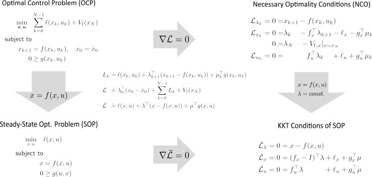
Figure 1: Relation of OCP and the corresponding Euler-Lagrange Equations with the SOP and the corresponding KKT conditions.

Invariance of $\bar{x}$ means

$$\bar{x}=f(\bar{x},\kappa_{\mathbb{X}_{f}}^{V_{\mathrm{f}}}(\bar{x})).$$ (11)

This invariance holds if and only if, for the considered EMPC scheme

$$\kappa_{\mathbb{X}_{f}}^{V_{\mathrm{f}}}(\bar{x})=\bar{u}.$$

Here, instead of providing fully detailed proofs, we focus on the crucial system-theoretic aspects.

Assumption 3 suggests to consider the NCO of the LQ approximation (8). Taking $(\bar{x},\bar{u})\in\textrm{int}{\mathcal{\,}}{\mathbb{Z}}$ into account those NCO entail

$$\bar{x} =A\bar{x}+B\bar{u},$$

$$\lambda_{k} =A^{\top}\lambda_{k+1}+Q\bar{x}+q,$$

$$0 =B^{\top}\lambda_{k}+R\bar{u}+r.$$

Assuming that $\det R\not=0$ and neglecting the first equation, we obtain

$$\lambda_{k} =\phantom{-}A^{\top}\lambda_{k+1}+Q\bar{x}+q,$$ (12a)

$$\bar{u} =-R^{-1}\left(B^{\top}\lambda_{k}+r\right).$$ (12b)

This in turn can be read as a linear uncontrolled system (12a) with a linear output equation (12b). Importantly, uniqueness of the steady state adjoint $\bar{\lambda}$ and controllability of $(A,B)$ ($\Leftrightarrow$ observability of $(A^{\top},B^{\top})$) imply that $\lambda_{k}=\lambda_{k+1}=\bar{\lambda}$ is the only solution (12), see [19]. This shows that the closed-loop invariance condition (11) holds at $\bar{x}$ if and only if the optimal adjoint satisfies $\lambda^{\star}_{0}(\bar{x})=\bar{\lambda}$, i.e., if the state initial condition is $\bar{x}$ then that adjoint at time $0$ is $\bar{\lambda}$.

Now, consider the boundary conditions of the adjoint $\lambda$ as given in (9d). We start with case (ii), i.e., $V_{\mathrm{f}}(x_{N})=0$, $\mathbb{X}_{\mathrm{f}}=\mathbb{R}^{n_{x}}$ and have $\lambda_{N}=0$. This implies

$$\lambda_{k}=A^{\top}\lambda_{k+1}+Q\bar{x}+q,\qquad\lambda_{N}=0.$$

If $\lambda_{0}=\bar{\lambda}$ would hold then the linearity of the adjoint dynamics implies for all $k\in\mathbb{I}_{[0,N]}$ that $\lambda_{k}\equiv\bar{\lambda}$. This, however, contradicts the boundary constraint $\lambda_{N}=0$. Hence the adjoint has to leave the optimal steady state value directly in the first time-step. A formal proof of the above considerations can be found in [19]. Moreover, we remark without further elaboration that in the continuous-time case, the mismatch between dual terminal constraint at $\lambda_{N}=0$ leads to a small-scale periodic orbit which appears in closed loop, cf. [40]. Finally, in case of singular OCPs with $\det\bar{L}_{uu}=\det R=0$ the NCOs do not directly allow to infer the controls. One can arrive at one of two cases:

• For sufficiently long horizons, the open-loop optimal solution reach the optimal steady state $(\bar{x},\bar{u})$ exactly. In this case, one says that the turnpike at $(\bar{x},\bar{u})$ is exact. Moreover, one can show even with $\lambda_{N}=0$ (i.e. no terminal penalty) invariance of $\bar{x}$ under the EMPC feedback law and thus also asymptotic stability is attained. We refer to [12] for a detailed analysis of the continuous-time case.

• Despite the OCP being singular, for all finite horizons, the open-loop optimal solution get only close to the optimal steady state $(\bar{x},\bar{u})$, i.e., the turnpike is not exact but approximate [11]. Without any terminal penalty or primal terminal constraint, one cannot expect to achieve asymptotic stability in this case.

In case (iii), i.e., $V_{\mathrm{f}}(x_{N})=\bar{\lambda}^{\top}x_{N}$, $\mathbb{X}_{\mathrm{f}}=\mathbb{R}^{n_{x}}$ we arrive at

$$\lambda_{k} =\phantom{-}A^{\top}\lambda_{k+1}+Q\bar{x}+q,\quad\lambda_{N}=\bar{\lambda},$$

$$\bar{u} =-R^{-1}\left(B^{\top}\lambda_{k}+r\right).$$

In this case, the boundary condition $\lambda_{N}=\bar{\lambda}$ prevents the adjoint from leaving $\bar{\lambda}$.

Finally, for scheme (i), i.e., $V_{\mathrm{f}}(x_{N})=0$, $\mathbb{X}_{\mathrm{f}}=\{\bar{x}\}$, there is no boundary constraint for the adjoint. Here invariance of $\bar{x}$ is directly enforced by the primal terminal constraint $x_{N}=\bar{x}$. Slightly simplifying, one may state that the local curvature implied by the strict dissipation inequality (4b) makes staying at $\bar{x}$ cheaper than leaving and returning. Moreover, one can also draw upon the stability result from Theorem 1 to conclude that the invariance condition (11) holds, which in our setting implies that the adjoint is also at steady state $\bar{\lambda}$.

III-D Bounds on the Stabilizing Horizon Length

The next aspect we are interested in analyzing is the minimal stabilizing horizon length induced by the differences in Schemes (i) – (iii).

To this end, recall Assumption 2 (i), which requires exponential reachability of $\bar{x}$ from all $x_{0}\in\mathbb{X}_{0}$. This also means that the set $\mathbb{X}_{0}$ is controlled forward invariant. Put differently, for all $x_{0}\in\mathbb{X}_{0}$, there exist infinite-horizon controls such that the solutions stay in $\mathbb{X}_{0}$ for all times.

Similarly to the feasible sets $\mathbb{F}_{\bar{x}}^{0}(N,x)$, $\mathbb{F}_{\mathbb{R}^{n_{x}}}^{0}(N,x)$ and $\mathbb{F}_{\mathbb{R}^{n_{x}}}^{\bar{\lambda}^{\top}x}(N,x)$ we use super- and sub-scripts to distinguish the EMPC feedback laws $\kappa_{\bar{x}}^{0}(N,x)$, $\kappa_{\mathbb{R}^{n_{x}}}^{0}(N,x)$ and $\kappa_{\mathbb{R}^{n_{x}}}^{\bar{\lambda}^{\top}x}(N,x)$ for the three EMPC schemes. Moreover, using the arguments $N,x$ we highlight the dependence of the feedback on the horizon length $N$.

In case of Scheme (i), the computation of the minimal stabilizing horizon length can be formalized via the folllowing bi-level optimization problem

$$N^{0}_{\bar{x}}=\min_{N\in\mathbb{N}} ~{}N$$ (13a)

subject to $$\quad\mathbb{F}_{\bar{x}}^{0}(N,x)\not=\emptyset, \quad\forall\,x \in\mathbb{X}_{0},$$ (13b)

$$\quad f(x,\kappa_{\bar{x}}^{0}(N,x))\in\mathbb{X}_{0}, \quad\forall\,x \in\mathbb{X}_{0}.$$ (13c)

The first constraint (13b) encodes the observation that for Scheme (i) feasibility implies closed-loop stability of $\bar{x}$. The second constraint (13c) encodes that for any NMPC scheme to be stabilizing the set $\mathbb{X}_{0}$ is indeed rendered forward invariant by the NMPC feedback. The latter constraint implies a bi-level optimization nature of the problem: in order to solve (14) / (15), one needs to simulate the closed EMPC loop to obtain the feedback in (13c).

Note that this constraint will not be (strongly) active in case of a terminal point constraint. This can be seen from the fact that leaving (13c) out will not change the value of $N^{0}_{\bar{x}}$. The reason is that, provided the problem was feasible at the previous time step, the point-wise terminal constraint makes it immediate to construct a feasible guess for the NMPC problem (1). Therefore, (13) can be rewritten equivalently as a single-level optimization problem. Here we include this constraint to simplify a comparison of the three NMPC schemes.

Notice that the problem above, if solved to global optimality, provides the true minimal stabilizing horizon length for Scheme (i). Yet, solving it is complicated by the fact that $\mathbb{F}_{\bar{x}}^{0}(N,x_{0})\not=\emptyset,\ \forall\,x_{0}\in\mathbb{X}_{0}$ is an infinite dimensional constraint. Moreover, as long as one does not tighten exponential reachablity to finite-time reachability of $\bar{x}$ from all $x_{0}\in\mathbb{X}_{0}$, the optimal solution to (13) might be $N^{0}_{\bar{x}}=\infty$.

The straightforward counterparts to (13) for Schemes (ii) and (iii) read

$$N_{\mathbb{R}^{n_{x}}}^{0}=\min_{N\in\mathbb{N}} ~{}N$$ (14a)

subject to $$\quad\mathbb{F}_{\mathbb{R}^{n_{x}}}^{0}(N,x)\not=\emptyset, \quad\forall\,x \in\mathbb{X}_{0},$$ (14b)

$$\quad f(x,\kappa_{\mathbb{R}^{n_{x}}}^{0}(N,x))\in\mathbb{X}_{0}, \quad\forall\,x \in\mathbb{X}_{0},$$ (14c)

respectively,

$$N_{\mathbb{R}^{n_{x}}}^{\bar{\lambda}^{\top}x}=\min_{N\in\mathbb{N}} ~{}N$$ (15a)

subject to $$\quad\mathbb{F}_{\mathbb{R}^{n_{x}}}^{\bar{\lambda}^{\top}x}(N,x)\not=\emptyset, \quad\forall\,x \in\mathbb{X}_{0},$$ (15b)

$$\quad f(x,\kappa_{\mathbb{R}^{n_{x}}}^{\bar{\lambda}^{\top}x}(N,x))\in\mathbb{X}_{0}, \quad\forall\,x \in\mathbb{X}_{0}.$$ (15c)

If, in all problems (13)–(15), the forward invariance constraints (13c)–(15c) are inactive—which is indeed the case for (13c) or if there are no state constraints implied by $\mathbb{Z}$—, the following relation is easily derived:

$$N_{\mathbb{R}^{n_{x}}}^{0}=N_{\mathbb{R}^{n_{x}}}^{\bar{\lambda}^{\top}x}\leq N^{0}_{\bar{x}}.$$

At first sight, this relation appears to be a rigorous advantage of Schemes (ii) and (iii). However, for those schemes there is, to the best of our knowledge, no general guarantee that recursive feasibility alone implies asymptotic properties. As a matter of fact, Scheme (ii) only admits practical asymptotic stability properties. Hence for Schemes (ii) and (iii) the horizon length computed via (14) or (15) constitutes a lower bound on the minimal stabilizing horizon length of the underlying schemes. Finally, we remark that while for (13) the invariance constraint (13c) is inactive, in (14) and (15) the feasibility set constraints (14b) and (15b) are inactive. The reason is that Assumption 2(i) implies that $\mathbb{X}_{0}$ is a controlled forward invariant set. In turn, this directly implies that for all $x\in\mathbb{X}_{0}$ and any $N\in\mathbb{N}^{+}$ the feasibility sets in (14b) and (15b) are non-empty as there are no primal terminal constraints in the underlying OCPs. However, inactivity of these constraints does not provide a handle to overcome the bi-level optimization nature of (14) and (15). Hence we turn towards an approximation procedure.

Computational Approximation

To approximate the solution to (13), we fix a set of initial conditions

$$\tilde{\mathbb{X}}_{0}\doteq\{x_{0}^{j},\quad j=1,\dots,M\}.$$

For all samples $x_{0}^{j}$, we solve the minimum-time problem

$$N_{\bar{x}}^{0}(x_{0}^{j})\doteq\min_{\boldsymbol{x},\boldsymbol{u},N}\ \ N$$ (16a)

subject to $$x_{0}=x_{0}^{j},$$ (16b)

$$x_{k+1}=f(x_{k},u_{k}), k\in\mathbb{I}_{[0,N-1]},$$ (16c)

$$g(x_{k},u_{k})\leq 0, k\in\mathbb{I}_{[0,N]},$$ (16d)

$$x_{N}=\bar{x}.$$ (16e)

By virtue of Bellman’s optimality principle, the minimum-time problem defined above allows one to conclude the behaviour of the closed-loop with primal terminal constraint. Whenever no solution to this problem is found, we define $N_{\bar{x}}^{0}(x_{0}^{j})\doteq\infty$. Eventually, an approximation of (13) is given by

$$N_{\bar{x}}^{0}\approx\max_{x_{0}^{j}\in\tilde{\mathbb{X}}_{0}}~{}N_{\bar{x}}^{0}(x_{0}^{j}),$$

provided that the samples $x_{0}^{j}$ are sufficiently dense and cover a sufficiently large subset of the x-projection of $\mathbb{Z}$. Observe that additional information is contained in the tuples $(x_{0}^{j},N_{\bar{x}}(x_{0}^{j}))$: large values of $N_{\bar{x}}(x_{0}^{j})$ indicate that reaching $\bar{x}$ from $x_{0}^{j}$ is difficult.

The conceptual counterpart to (16) for Schemes (ii) and (iii) is a forward simulation of the closed loop with $\dagger=\{0,\bar{\lambda}^{\top}x\}$ and

$$N_{\mathbb{R}^{n_{x}}}^{\dagger}(x_{0}^{j})\doteq\min_{N} ~{}~{}N$$ (17a)

subject to $$x_{0}=x_{0}^{j},$$ (17b)

$$x_{k+1}=f(x_{k},\kappa_{\mathbb{R}^{n_{x}}}^{\dagger}(N,x_{k})), k\in\mathbb{I}_{[0,N_{\mathrm{cl}}]},$$ (17c)

$$x_{N_{\mathrm{cl}}}\in\mathcal{B}_{\rho}(\bar{x}),$$ (17d)

where $\mathcal{B}_{\rho}$ denotes a ball of radius $\rho$ and $N_{\mathrm{cl}}$ denotes the closed-loop simulation horizon which should ideally be infinite, but can in practice only be finite. Obviously, the above problem requires one to solve a large number of OCPs when simulating the closed-loop. Moreover, one has to rigorously define the radius $\rho$, i.e., the accuracy by which the optimal steady-state should be attained. This approximation procedure leads to

$$N_{\mathbb{R}^{n_{x}}}^{\dagger}\approx\max_{x_{0}^{j}\in\tilde{\mathbb{X}}_{0}}~{}N_{\mathbb{R}^{n_{x}}}^{\dagger}(x_{0}^{j}),\qquad\dagger=\{0,\bar{\lambda}^{\top}x\}.$$

IV Simulation Example

We consider a system with state $x=\begin{bmatrix}x_{\mathrm{A}}&x_{\mathrm{B}}\end{bmatrix}^{\top}\in[0,1]^{2}$, control $u\in[0,20]$, stage cost and dynamics

$$\ell(x,u) =-2ux_{\mathrm{B}}+0.5u+0.1(u-12)^{2},$$ (18a)

$$f(x,u) =\begin{bmatrix}x_{\mathrm{A}}+0.01\,u\,(1-x_{\mathrm{A}})-0.12\,x_{\mathrm{A}}\\ x_{\mathrm{B}}+0.01\,u\,x_{\mathrm{B}}+0.12\,x_{\mathrm{A}}\end{bmatrix}.$$ (18b)

This example has also been considered in [19]. The optimal steady state is $\bar{x}^{\star}=[0.5,0.5]^{\top}$, $\bar{u}^{\star}=12$ with $\bar{\lambda}^{\star}=[-100,-200]^{\top}$.

We computed the stabilizing horizon length for the three economic NMPC variants and observed that for the two schemes without terminal constraints in case $V_{\mathrm{f}}(x)=\bar{\lambda}^{\top}x$ we obtain stability with $N=1$ for any $\rho>0$, while for $V_{\mathrm{f}}(x)=0$ the stabilizing horizon length is independent of the initial condition but depends on $\rho$ as displayed in Figure 2 (right). For the formulation with the terminal constraint $x_{N}=\bar{x}$, the stabilizing horizon length depends on the initial condition, as some initial conditions are potentially infeasible. We display the stability regions for several choices of $N$ in Figure 2 (left) and observe that for $N\geq 7$ stability is obtained for all feasible initial states. These results are also summarized in Table I.

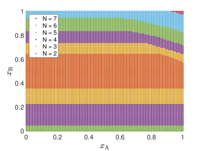
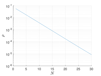
Figure 2: Stabilizing horizon length. Left graph: $N_{\bar{x}}^{0}$ as a function of the initial state. Right graph: $\rho$ as a function of $N$ for scheme (ii).

TABLE I: Numerical approximation results of the minimal stabilizing horizon length for (18).

EMPC		Minimal stabilizing	Eventual deviation
		horizon length for $x_{0}\in\tilde{\mathbb{X}}_{0}$	from $\bar{x}$
(i) $V_{\mathrm{f}}(x)=0$	$\mathbb{X}_{\mathrm{f}}=\{\bar{x}\}$	$N=7$	$0$
(ii) $V_{\mathrm{f}}(x)=0$	$\mathbb{X}_{\mathrm{f}}=\mathbb{R}^{n_{x}}$	$N\geq 1$	$<7.6\cdot 10^{-2}\ e^{-0.29N}$
(iii) $V_{\mathrm{f}}(x)=\bar{\lambda}^{\top}x$	$\mathbb{X}_{\mathrm{f}}=\mathbb{R}^{n_{x}}$	$N=1$	$0$

V Summary and Outlook

This chapter has compared three established schemes for economic NMPC

• $V_{\mathrm{f}}(x)=0$     and   $\mathbb{X}_{\mathrm{f}}=\{\bar{x}\}$;

• $V_{\mathrm{f}}(x)=0$     and   $\mathbb{X}_{\mathrm{f}}=\mathbb{R}^{n_{x}}$;

• $V_{\mathrm{f}}(x)=\bar{\lambda}^{\top}x$   and   $\mathbb{X}_{\mathrm{f}}=\mathbb{R}^{n_{x}}$;

with respect to different aspects:

• the role of primal and dual terminal constraints;

• the characteristics of the feasible set;

• the length of the stabilizing horizon.

On the considered example, the stabilizing horizon length improves from $N=7$ to $N=1$ from scheme (i) to scheme (iii). Hence, it turns out that the simple linear end penalty $V_{\mathrm{f}}(x)=\bar{\lambda}^{\top}x$ does not only help with respect to convergence to the optimal steady state, but also with respect to feasibility of the OCP for short horizon. Indeed, the numerical analysis of Section IV indicates that the effect of this terminal constraint on the minimal stabilizing horizon length is substantial as compared to the scheme with terminal constraint.

Notably, the results of [19] and [18] have also shown that optimal steady-state adjoint $\bar{\lambda}$ does not need to be known a-priori. In case of accurate models it can be inferred from open-loop predictions [19] and in case of model deficiencies it can be estimated from plant data [18]. However, a formal proof of supremacy in terms of closed-loop performance is currently not available. Moreover, the analysis of Section IV should be validated also on more challenging examples. Finally, we remark that the time-varying counterpart for the scheme with $V_{\mathrm{f}}(x)=\bar{\lambda}^{\top}x$ is still to be explored. Moreover, the preliminary analysis in terms of stabilizing horizon lengths for the different schemes could be extended using viability kernel concepts, see e.g. [4].

References

- [1] R. Amrit, J.B. Rawlings, and D. Angeli. Economic optimization using model predictive control with a terminal cost. Annual Reviews in Control, 35(2):178 – 186, 2011.
- [2] D. Angeli, R. Amrit, and J.B. Rawlings. On average performance and stability of economic model predictive control. IEEE Trans. Automat. Contr., 57(7):1615–1626, 2012.
- [3] D. Angeli and M.A. Müller. Economic model predictive control: Some design tools and analysis techniques. In Handbook of Model Predictive Control, pages 145–167. Springer, 2019.
- [4] A. Boccia, L. Grüne, and K. Worthmann. Stability and feasibility of state constrained MPC without stabilizing terminal constraints. Syst. Contr. Lett., 72:14–21, 2014.
- [5] A.E. Bryson. Dynamic Optimization. Addison-Wesley, Menlo Park, California, 1999.
- [6] D.A. Carlson, A. Haurie, and A. Leizarowitz. Infinite Horizon Optimal Control: Deterministic and Stochastic Systems. Springer Verlag, 1991.
- [7] J. De Schutter, M. Zanon, and M. Diehl. TuneMPC - A Tool for Economic Tuning of Tracking (N)MPC Problems. IEEE Control Systems Letters, 4(4):910–915, 2020.
- [8] M. Diehl, R. Amrit, and J.B. Rawlings. A Lyapunov function for economic optimizing model predictive control. IEEE Trans. Automat. Contr., 56(3):703–707, 2011.
- [9] R. Dorfman, P.A. Samuelson, and R.M. Solow. Linear Programming and Economic Analysis. McGraw-Hill, New York, 1958.
- [10] M. Ellis, H. Durand, and P.D. Christofides. A tutorial review of economic model predictive control methods. Journal of Process Control, 24(8):1156–1178, 2014.
- [11] T. Faulwasser and D. Bonvin. On the design of economic NMPC based on approximate turnpike properties. In Proc. of 54th IEEE Conference on Decision and Control, pages 4964 – 4970, Osaka, Japan, December 15-18 2015.
- [12] T. Faulwasser and D. Bonvin. Exact turnpike properties and economic NMPC. European Journal of Control, 35:34–41, May 2017.
- [13] T. Faulwasser, L. Grüne, J.-P. Humaloja, and M. Schaller. The interval turnpike property for adjoints. Pure and Applied Functional Analysis, 2020. Accepted.
- [14] T. Faulwasser, L. Grüne, and M. Müller. Economic nonlinear model predictive control: Stability, optimality and performance. Foundations and Trends in Systems and Control, 5(1):1–98, 2018.
- [15] T. Faulwasser and C.M. Kellett. On continuous-time infinite horizon optimal control – Dissipativity, stability and transversality. 2020. arxiv: 2001.09601.
- [16] T. Faulwasser, M. Korda, C.N. Jones, and D. Bonvin. On turnpike and dissipativity properties of continuous-time optimal control problems. Automatica, 81:297–304, April 2017.
- [17] T. Faulwasser and A. Murray. Turnpike properties in discrete-time mixed integer optimal control. IEEE Control Systems Letters, 2020. arxiv: 2002.02049.
- [18] T. Faulwasser and G. Pannocchia. Towards a unifying framework blending real-time optimization and economic model predictive control. Industrial and Chemical Engineering Research, 58(30):13583–13598, 2019.
- [19] T. Faulwasser and M. Zanon. Asymptotic stability of economic NMPC: The importance of adjoints. IFAC-PapersOnLine, 51(20):157–168, 2018.
- [20] L. Grüne. Economic receding horizon control without terminal constraints. Automatica, 49(3):725–734, 2013.
- [21] L. Grüne and M.A. Müller. On the relation between strict dissipativity and turnpike properties. Sys. Contr. Lett., 90:45 – 53, 2016.
- [22] L. Grüne and J. Pannek. Nonlinear Model Predictive Control: Theory and Algorithms. Communication and Control Engineering. Springer Verlag, 2nd edition edition, 2017.
- [23] L. Grüne, S. Pirkelmann, and M. Stieler. Strict dissipativity implies turnpike behavior for time-varying discrete time optimal control problems. In Control Systems and Mathematical Methods in Economics, pages 195–218. Springer, 2018.
- [24] L. Grüne, M. Schaller, and A. Schiela. Exponential sensitivity and turnpike analysis for linear quadratic optimal control of general evolution equations. Journal of Differential Equations, 2019.
- [25] L. Grüne and M. Stieler. A Lyapunov function for economic MPC without terminal conditions. In Proceedings of the 53rd IEEE Conference on Decision and Control, pages 2740–2745, December 2014.
- [26] J.V. Kadam and W. Marquardt. Integration of economical optimization and control for intentionally transient process operation. In R. Findeisen, F. Allgöwer, and L.T. Biegler, editors, Assessment and Future Directions of Nonlinear Model Predictive Control, volume 358 of Lecture Notes in Control and Information Sciences, pages 419–434. Springer Berlin Heidelberg, 2007.
- [27] L.W. McKenzie. Turnpike theory. Econometrica: Journal of the Econometric Society, 44(5):841–865, 1976.
- [28] P. Moylan. Dissipative Systems and Stability. http://www.pmoylan.org, 2014.
- [29] M.A. Müller, D. Angeli, and F. Allgöwer. On necessity and robustness of dissipativity in economic model predictive control. IEEE Trans. Automat. Contr., 60(6):1671–1676, 2015.
- [30] J. Rawlings and R. Amrit. Optimizing process economic performance using model predictive control. In L. Magni, D. Raimondo, and F. Allgöwer, editors, Nonlinear Model Predictive Control - Towards New Challenging Applications, volume 384 of Lecture Notes in Control and Information Sciences, pages 119–138. Springer Berlin, 2009.
- [31] J.B. Rawlings, D.Q. Mayne, and M. Diehl. Model Predictive Control: Theory, Computation, and Design. Nob Hill Publishing, Madison, WI, 2017.
- [32] E. Trélat and E. Zuazua. The turnpike property in finite-dimensional nonlinear optimal control. Journal of Differential Equations, 258(1):81–114, 2015.
- [33] J. von Neumann. Über ein ökonomisches Gleichungssystem und eine Verallgemeinerung des Brouwerschen Fixpunktsatzes. In K. Menger, editor, Ergebnisse eines Mathematischen Seminars. 1938.
- [34] L. Weiss. Controllability, realization and stability of discrete-time systems. SIAM Journal on Control, 10(2):230–251, 1972.
- [35] J.C. Willems. Least squares stationary optimal control and the algebraic riccati equation. IEEE Trans. Aut. Contr., 16(6):621–634, 1971.
- [36] J.C. Willems. Dissipative dynamical systems part i: General theory. Archive for Rational Mechanics and Analysis, 45(5):321–351, 1972.
- [37] J.C. Willems. Dissipative dynamical systems part ii: Linear systems with quadratic supply rates. Archive for Rational Mechanics and Analysis, 45(5):352–393, 1972.
- [38] J.C. Willems. Dissipative dynamical systems. European Journal of Control, 13(2-3):134–151, 2007.
- [39] M. Zanon. A Gauss-Newton-Like Hessian Approximation for Economic NMPC. IEEE Trans. Aut. Contr. (submitted) available at https://arxiv.org/abs/2007.13519.
- [40] M. Zanon and T. Faulwasser. Economic MPC without terminal constraints: Gradient-correcting end penalties enforce stability. Journal of Process Control, 63:1–14, 3 2018.
- [41] M. Zanon, S. Gros, and M. Diehl. A Lyapunov Function for Periodic Economic Optimizing Model Predictive Control. In Proceedings of the 52nd Conference on Decision and Control (CDC), pages 5107–5112, 2013.
- [42] M. Zanon, S. Gros, and M. Diehl. Indefinite linear MPC and approximated economic MPC for nonlinear systems. Journal of Process Control, 24(8):1273–1281, 2014.
- [43] M. Zanon, S. Gros, and M. Diehl. A tracking MPC formulation that is locally equivalent to economic MPC. Journal of Process Control, 45:30–42, 2016.
- [44] M. Zanon, S. Gros, and M. Diehl. A Periodic Tracking MPC that is Locally Equivalent to Periodic Economic MPC. In Proceedings of the 2017 IFAC World Congress, volume 50, pages 10711–10716, 2017.
- [45] M. Zanon, L. Grüne, and M. Diehl. Periodic optimal control, dissipativity and MPC. IEEE Trans. Aut. Contr., 62(6):2943–2949, 2017.