Cost of quantum entanglement simplified

Abstract

Quantum entanglement is a key physical resource in quantum information processing that allows for performing basic quantum tasks such as teleportation and quantum key distribution, which are impossible in the classical world. Ever since the rise of quantum information theory, it has been an open problem to quantify entanglement in an information-theoretically meaningful way. In particular, every previously defined entanglement measure bearing a precise information-theoretic meaning is not known to be efficiently computable, or if it is efficiently computable, then it is not known to have a precise information-theoretic meaning. In this paper, we meet this challenge by introducing an entanglement measure that has a precise information-theoretic meaning as the exact cost required to prepare an entangled state when two distant parties are allowed to perform quantum operations that completely preserve the positivity of the partial transpose. Additionally, this entanglement measure is efficiently computable by means of a semi-definite program, and it bears a number of useful properties such as additivity and faithfulness. Our results bring key insights into the fundamental entanglement structure of arbitrary quantum states, and they can be used directly to assess and quantify the entanglement produced in quantum-physical experiments.

LABEL:FirstPage1 LABEL:LastPage#110

Introduction.—Quantum entanglement is a fundamental property of quantum states that has no classical analog. As famously remarked by Schrödinger Schrödinger (1935), it is “the characteristic trait of quantum mechanics, the one that enforces its entire departure from classical lines of thought.” Einstein, Podolsky, and Rosen were confounded by entanglement Einstein et al. (1935), and based on this, proposed a theory alternative to quantum mechanics, which was later ruled out by a theoretical proposal of Bell Bell (1964) and experimental confirmations of Bell’s test Aspect et al. (1981); Hensen et al. (2015); Giustina et al. (2015); Shalm et al. (2015).

The aforementioned early work on understanding entanglement ended up being foundational for the modern field of quantum information science Nielsen and Chuang (2000); Wilde (2017), whose goal is to harness the strange properties of quantum states for information processing tasks that are not possible in the classical world. Due to seminal work by Bennett et al., we now understand quantum entanglement to be the enabling fuel for a variety of quantum protocols such as teleportation Bennett et al. (1993), dense coding Bennett and Wiesner (1992), and quantum key distribution Bennett and Brassard (1984); Ekert (1991).

In the fundamental protocols mentioned above, it is required for the entangled states being consumed to be in a pure form, known as maximally entangled states. However, in experimental practice, quantum states do not come in this pure variety, but instead are produced as mixtures of pure states. As such, a key goal of the resource theory of entanglement Bennett et al. (1996a) is to understand how well mixed quantum states can be converted to pure maximally entangled states and vice versa, by means of “free” physical operations that do not increase entanglement. Motivated by the “distant laboratories paradigm,” in which the two parties holding shares of a quantum state are spatially separated, one set of physical operations that is reasonable to allow for free consists of those that can be implemented by local operations and classical communication (LOCC). The characterization of entanglement as a resource in practical settings is also rooted in this distant laboratories paradigm.

There are two primary operational ways for quantifying entanglement in a two-party quantum state $\rho_{AB}$: the first is known as distillable entanglement Bennett et al. (1996a) and the second is known as entanglement cost Bennett et al. (1996a); Hayden et al. (2001). In the first approach, one is interested to know the largest rate at which maximally entangled states can be distilled by means of LOCC from the state $\rho_{AB}$. In the second, one is interested to know the smallest rate at which maximally entangled states are required to prepare the state $\rho_{AB}$ by means of LOCC. There are a number of technical variations of each task that have been considered Bennett et al. (1996a); Terhal and Horodecki (2000); Hayden et al. (2001); Buscemi and Datta (2011), involving one or multiple copies of the state $\rho_{AB}$, or for the task to be accomplished exactly or with some error tolerance. So far, beyond the case of pure states Bennett et al. (1996b), it has been a great challenge since the publication of the seminal work in Bennett et al. (1996a) to characterize the distillability and cost of quantum entanglement. Much of the progress during the past two decades has to do with finding alternative entanglement measures that bound entanglement distillability or cost, while possessing properties that are generally agreed upon to be reasonable Vedral and Plenio (1998); Rains (1999, 2001); Vidal and Werner (2002); Christandl and Winter (2004); Plenio (2005); Plenio and Virmani (2007); Horodecki et al. (2009); Wang and Duan (2016, 2017). Even many of the measures that have been defined are known to be difficult to compute Huang (2014).

Due to the aforementioned challenges associated with mixed-state entanglement and the set LOCC in general Chitambar et al. (2014), researchers have looked in other directions in order to understand the nature of entanglement. One approach was pioneered in Rains (2001), with the introduction of another set of free operations that “completely preserve the positivity of the partial transpose” Chitambar et al. (2017) (we explain the precise meaning of this term later). This set (abbreviated by C-PPT-P) has been considered in prior work Eggeling et al. (2001); Audenaert et al. (2003); Horodecki et al. (2002); Plenio (2005); Wang and Duan (2017) on entanglement theory for at least two reasons:

1. The mathematical structure of LOCC is difficult to work with and so enlarging the set to a more mathematically tractable set allows for providing bounds on what one could accomplish with LOCC. That is, such free operations provide accessible estimates of the capabilities of LOCC in entanglement manipulation.

2. The free states that correspond to this enlarged set, known as positive partial transpose (PPT) states, in any case do not have any useful entanglement on their own (in the sense that it is impossible to distill maximally entangled states from them at a non-trivial rate via LOCC).

As observed in Rains (2001), an advantage of the set C-PPT-P over LOCC is that performing optimizations over it allows for incorporating the tools of semi-definite programming.

One key problem that has remained open for many years now is to characterize the exact entanglement cost of a quantum state $\rho_{AB}$ when C-PPT-P operations are allowed for free, which is equal to the minimum rate at which entanglement is required to prepare many perfect and identical copies of $\rho_{AB}$ by means of these free operations. The optimal rate is known as the PPT exact entanglement cost. The problem was formalized in Audenaert et al. (2003), where some bounds on this quantity were given and some partial solutions were presented. The problem was considered further in Matthews and Winter (2008), which however focused mainly on transformations of pure entangled states.

In this paper, we determine the PPT exact entanglement cost of an arbitrary two-party quantum state, thus closing a longstanding investigation in entanglement theory. We find that the solution is given by a new entanglement measure, which we call $\kappa$-entanglement. The $\kappa$-entanglement can be calculated by means of a semi-definite program Boyd and Vandenberghe (2004), implying that it can be efficiently calculated in time polynomial in the dimension of the state on which it is being evaluated Khachiyan (1980); Arora et al. (2005); Arora and Kale (2007); Arora et al. (2012); Lee et al. (2015). These two properties single out the $\kappa$-entanglement as the first entanglement measure that has a concrete information-theoretic meaning while being efficiently calculable. The $\kappa$-entanglement also bears a number of desirable properties, including additivity, normalization, and faithfulness, which we expand upon later. It is neither convex nor monogamous Terhal (2004), which calls into question whether it is truly necessary for an entanglement measure to satisfy either of these properties.

Our results on $\kappa$-entanglement of quantum states bring new insights regarding the structure of quantum entanglement as a physical resource. For one, they demonstrate that entanglement can be quantified in a precise and physically relevant operational scenario. Furthermore, they call into question whether properties such as monogamy or convexity are really required for entanglement measures, in light of the fact that $\kappa$-entanglement does not have these properties while at the same time having the aforementioned operational meaning.

We now begin the more technical part of our paper by giving some background, defining the PPT exact entanglement cost and $\kappa$-entanglement of a quantum state, and justifying how these quantities are equal. We note here that all mathematical proofs of the various statements and properties summarized in this paper are given in the Supplementary Material Wang and Wilde (2020), which also includes the following references not mentioned in the main text Nielsen (1999); Hayashi (2006); Yue and Chitambar (2018); Horodecki and Horodecki (1999); Watrous (2018); Furrer et al. (2011); Ishizaka (2004); Coffman et al. (2000); Koashi and Winter (2004); Dell’Antonio (1967); Reed and Simon (1978); Gour and Scandolo (2019); Wang and Wilde (2018); Brandao (2005).

Let us first recall some basic elements of quantum information. A two-party or bipartite quantum state $\rho_{AB}$ is a unit trace, positive semi-definite operator acting on a tensor-product Hilbert space $\mathcal{H}_{A}\otimes\mathcal{H}_{B}$. We say that Alice possesses system $A$ and Bob system $B$, and we imagine that Alice and Bob are located in distant laboratories. Such a state is separable Werner (1989) if there exists a probability distribution $p_{X}$ and sets of states $\left\{\sigma_{A}^{x}\right\}_{x}$ and $\{\tau_{B}^{x}\}_{x}$ such that

$$\rho_{AB}=\sum_{x}p_{X}(x)\sigma_{A}^{x}\otimes\tau_{B}^{x}.$$ (1)

If $\rho_{AB}$ cannot be written in the above way, then it is entangled Werner (1989).

It is a difficult (NP-hard) computational problem to decide whether an arbitrary quantum state is separable or entangled Gurvits (2003); Gharibian (2010). As such, researchers have sought out simpler, “one-way” criteria to classify entanglement of quantum states. Possibly the simplest such criterion is the positive partial transpose criterion Peres (1996); Horodecki et al. (1996). To define this, recall that the partial transpose, with respect to a given orthonormal basis $\{|i\rangle_{B}\}_{i}$, is defined as the following linear map:

$$T_{B}(X_{AB}):=\sum_{i,j}\left(I_{A}\otimes|i\rangle\langle j|_{B}\right)X_{AB}\left(I_{A}\otimes|i\rangle\langle j|_{B}\right),$$ (2)

which we also write as $X_{AB}^{T_{B}}\equiv T_{B}(X_{AB})$. An operator $X_{AB}$ has positive partial transpose (PPT) if $T_{B}(X_{AB})$ is positive semi-definite. By inspecting definitions, we conclude that if a bipartite state is separable, then it is a PPT state. By contrapositive, we conclude that a bipartite state is entangled if it has a negative partial transpose. The PPT criterion is one-way in the sense that there exist entangled PPT states Horodecki et al. (1998).

A quantum channel is a completely positive trace-preserving map, and a bipartite quantum channel $\mathcal{N}_{AB\rightarrow A^{\prime}B^{\prime}}$ accepts input systems $A$ and $B$ and outputs $A^{\prime}$ and $B^{\prime}$, where one party Alice possesses $A$ and $A^{\prime}$ and another party Bob possesses $B$ and $B^{\prime}$. A bipartite quantum channel $\mathcal{N}_{AB\rightarrow A^{\prime}B^{\prime}}$ is completely positive-partial-transpose preserving Rains (2001), abbreviated as C-PPT-P, if the map $T_{B^{\prime}}\circ\mathcal{N}_{AB\rightarrow A^{\prime}B^{\prime}}\circ T_{B}$ is completely positive.

In the resource theory of NPT (non-positive partial transpose) entanglement, the free operations allowed are C-PPT-P bipartite channels and the free states are PPT states, and one of the main goals is to determine if one bipartite state can be converted to another either exactly or approximately by means of the free operations. The particular task of interest to us here is the PPT exact entanglement cost.

One-shot exact entanglement cost.—We begin by defining the one-shot PPT exact entanglement cost of a bipartite state $\rho_{AB}$ as the logarithm of the minimum Schmidt rank of a maximally entangled state that is required to prepare $\rho_{AB}$ by means of a C-PPT-P channel:

$$E_{\operatorname{PPT}}^{(1)}(\rho_{AB}):=\log_{2}\inf_{d\in\mathbb{N},\Lambda\in\operatorname{PPT}}\left\{d:\rho_{AB}=\Lambda_{\hat{A}\hat{B}\rightarrow AB}(\Phi_{\hat{A}\hat{B}}^{d})\right\},$$

where $\Lambda\in\operatorname{PPT}$ is a shorthand for $\Lambda$ being a C-PPT-P bipartite channel and the maximally entangled state $\Phi_{\hat{A}\hat{B}}^{d}$ is defined as

$$\Phi_{\hat{A}\hat{B}}^{d}:=\frac{1}{d}\sum_{i,j}|i\rangle\langle j|_{\hat{A}}\otimes|i\rangle\langle j|_{\hat{B}},$$ (3)

with $\{|i\rangle_{\hat{A}}\}_{i}$ and $\{|i\rangle_{\hat{B}}\}_{i}$ orthonormal bases. The (asymptotic) PPT exact entanglement cost of $\rho_{AB}$ is defined as

$$E_{\operatorname{PPT}}(\rho_{AB}):=\limsup_{n\rightarrow\infty}\frac{1}{n}E_{\operatorname{PPT}}^{(1)}(\rho_{AB}^{\otimes n}).$$ (4)

By building on earlier results from Audenaert et al. (2003); Matthews and Winter (2008), our first result is for the one-shot PPT exact entanglement cost:

Proposition 1

For a given bipartite quantum state $\rho_{AB}$, its one-shot PPT exact entanglement cost is given by

$$E_{\operatorname{PPT}}^{(1)}(\rho_{AB})=\\ \inf\left\{\begin{array}[c]{c}\log_{2}m:G_{AB}\geq 0,\ \operatorname{Tr}[G_{AB}]=1,\\ -\left(m-1\right)G_{AB}^{T_{B}}\leq\rho_{AB}^{T_{B}}\leq\left(m+1\right)G_{AB}^{T_{B}},m\in\mathbb{N}\end{array}\right\}.$$ (5)

The proof of this result involves an achievability and optimality part. The achievability part constructs the channel $\Lambda_{\hat{A}\hat{B}\rightarrow AB}\in\operatorname{PPT}$ as the following measure-prepare procedure:

$$\Lambda_{\hat{A}\hat{B}\rightarrow AB}(\omega_{\hat{A}\hat{B}}):=\rho_{AB}\operatorname{Tr}[\Phi_{\hat{A}\hat{B}}^{m}\omega_{\hat{A}\hat{B}}]\\ +G_{AB}\operatorname{Tr}[\left(I_{\hat{A}\hat{B}}-\Phi_{\hat{A}\hat{B}}^{m}\right)\omega_{\hat{A}\hat{B}}],$$ (6)

for $G_{AB}$ a quantum state satisfying $-\left(m-1\right)G_{AB}^{T_{B}}\leq\rho_{AB}^{T_{B}}\leq\left(m+1\right)G_{AB}^{T_{B}}$. That $\Lambda_{\hat{A}\hat{B}\rightarrow AB}$ is a quantum channel follows immediately from its construction, and that $\Lambda_{\hat{A}\hat{B}\rightarrow AB}\in\operatorname{PPT}$ follows from the constraint on $G_{AB}$. For the optimality part, we exploit the symmetry of the maximally entangled state $\Phi_{\hat{A}\hat{B}}^{d}$, that it is invariant under the unitary channel $\left(U\otimes\overline{U}\right)\left(\cdot\right)\left(U\otimes\overline{U}\right)^{{\dagger}}$ for an arbitrary unitary $U$, in order to constrain the set of channels that we have to consider for the PPT exact entanglement cost. Then by applying the constraint that $\Lambda_{\hat{A}\hat{B}\rightarrow AB}\in\operatorname{PPT}$, it follows that the constructed channel is optimal.

$\kappa$-entanglement.—The bottleneck of solving the PPT entanglement cost of a general bipartite state lies in determining the regularization of the one-shot cost, which involves evaluating the limit of a series of optimization problems. To overcome this difficulty, we introduce an efficiently computable entanglement measure, called $\kappa$-entanglement, defined as

$$E_{\kappa}(\rho_{AB}):=\log_{2}\inf_{S_{AB}\geq 0}\left\{\operatorname{Tr}[S_{AB}]:-S_{AB}^{T_{B}}\leq\rho_{AB}^{T_{B}}\leq S_{AB}^{T_{B}}\right\}.$$

In particular, $E_{\kappa}$ can be computed by means of a semi-definite program (SDP) Vandenberghe and Boyd (1996) (see Section B.2 of Wang and Wilde (2020) for details). SDPs can be computed efficiently by polynomial-time algorithms Khachiyan (1980); Arora et al. (2005); Arora and Kale (2007); Arora et al. (2012); Lee et al. (2015) and are often applied in quantum information (e.g., Fletcher et al. (2007); Watrous (2009); Leung and Matthews (2015); Lami et al. (2018); Fang et al. (2020); Wang (2018); Wang et al. (2020, 2019)). The CVX software Grant and Boyd (2008) allows one to compute SDPs in practice.

By observing that $\kappa$-entanglement is a relaxation of the one-shot cost in Proposition 1 up to small corrections, we arrive at the following bounds on the one-shot exact entanglement cost:

Proposition 2

For a bipartite state $\rho_{AB}$, we have

$$\log_{2}\!\left(2^{E_{\kappa}(\rho_{AB})}-1\right)\leq E_{\operatorname{PPT}}^{(1)}(\rho_{AB})\leq\log_{2}\!\left(2^{E_{\kappa}(\rho_{AB})}+2\right).$$ (7)

This result gives a tight and efficiently computable bound for the one-shot PPT exact entanglement cost in terms of $\kappa$-entanglement. A rigorous proof can be found in Wang and Wilde (2020). Thus, the inequality in Proposition 2 demonstrates that the $\kappa$-entanglement is closely related to the one-shot PPT exact entanglement cost, and as both the operational quantity $E_{\operatorname{PPT}}^{(1)}(\rho_{AB})$ and the entanglement measure $E_{\kappa}(\rho_{AB})$ become larger, the gap between them disappears.

In addition to being efficiently calculable by means of a semi-definite program, the $\kappa$-entanglement possesses several properties desirable for an entanglement measure, including monotonicity under selective C-PPT-P operations, additivity, faithfulness, and normalization. We elaborate on each of these briefly now. The monotonicity is the following inequality:

$$E_{\kappa}(\rho_{AB})\geq\sum_{x:p(x)>0}p(x)E_{\kappa}(\rho_{A^{\prime}B^{\prime}}^{x}),$$ (8)

where $p(x):=\operatorname{Tr}[\mathcal{P}_{AB\rightarrow A^{\prime}B^{\prime}}^{x}(\rho_{AB})]$, the set $\{\mathcal{P}_{AB\rightarrow A^{\prime}B^{\prime}}^{x}\}_{x}$ consists of completely positive, trace non-increasing, C-PPT-P maps such that $\sum_{x}\mathcal{P}_{AB\rightarrow A^{\prime}B^{\prime}}^{x}$ is trace preserving, and $\rho_{A^{\prime}B^{\prime}}^{x}:=\mathcal{P}_{AB\rightarrow A^{\prime}B^{\prime}}^{x}(\rho_{AB})/p(x)$. The inequality in (8) asserts that $\kappa$-entanglement does not increase on average under the action of selective C-PPT-P operations, which include selective LOCC operations as a special case. Additivity is the following statement, which is critical for establishing one of the key results of our paper:

$$E_{\kappa}(\omega_{A_{1}A_{2}:B_{1}B_{2}})=E_{\kappa}(\rho_{A_{1}B_{1}})+E_{\kappa}(\theta_{A_{2}B_{2}}),$$ (9)

where $\omega_{A_{1}A_{2}:B_{1}B_{2}}:=\rho_{A_{1}B_{1}}\otimes\theta_{A_{2}B_{2}}$ and $\rho_{A_{1}B_{1}}$ and $\theta_{A_{2}B_{2}}$ are quantum states. Faithfulness is that $E_{\kappa}(\rho_{AB})=0$ if and only if $\rho_{AB}$ is a PPT state. Finally, normalization is that $E_{\kappa}(\Phi_{AB}^{d})=\log_{2}d$ for $\Phi_{AB}^{d}$ a maximally entangled state of the form in (3). Proofs of the properties above are provided in Wang and Wilde (2020).

Exact entanglement cost.—The PPT exact entanglement cost ${E_{\operatorname{PPT}}}$ has been a longstanding open question since it was first introduced in Audenaert et al. (2003). The previously best known upper and lower bounds Audenaert et al. (2003) are tight for general Werner states, but they are not tight in general. The difficulty of determining ${E_{\operatorname{PPT}}}$ comes from the fact that the one-shot cost is not an SDP, and its regularization makes the problem more intractable. However, by utilizing the techniques of semi-definite optimization and relaxation, we prove that the asymptotic exact entanglement cost of a state $\rho_{AB}$ is given by ${E_{\kappa}}(\rho_{AB})$. Specifically, by exploiting (7), the definition of PPT exact entanglement cost in (4), and the additivity of $\kappa$-entanglement in (9), we arrive at one of our core contributions:

Theorem 1

The PPT exact entanglement cost of an arbitrary bipartite state $\rho_{AB}$ is given by

$$E_{\operatorname{PPT}}(\rho_{AB})=E_{\kappa}(\rho_{AB}).$$ (10)

This result has two important consequences. First, it demonstrates that $\kappa$-entanglement precisely determines the PPT exact entanglement cost of an arbitrary quantum state. Notably, this is the first time that an entanglement measure for general bipartite states has been proven not only to possess a direct operational meaning but also to be efficiently computable, thus solving a question that has remained open since the inception of entanglement theory over two decades ago. Second, note that ${E_{\kappa}}$ is additive (cf., Eq. (9)), so that Theorem 1 implies that the PPT exact entanglement cost is additive in general:

$${E_{\operatorname{PPT}}}(\rho_{AB}\otimes\omega_{A^{\prime}B^{\prime}})={E_{\operatorname{PPT}}}(\rho_{AB})+{E_{\operatorname{PPT}}}(\omega_{A^{\prime}B^{\prime}}).$$ (11)

Based on Theorem 1, we further show that the PPT exact entanglement cost violates the convexity and monogamy inequalities, which gives insight to the fundamental structure of entanglement. Recall that for an entanglement measure $E$, convexity is the following statement:

$$E(\overline{\rho}_{AB})\leq\sum_{z}p(z)E(\rho_{AB}^{z}),$$ (12)

where $p(z)$ is a probability distribution, $\left\{\rho_{AB}^{z}\right\}_{z}$ is a set of states, and $\overline{\rho}_{AB}:=\sum_{z}p(z)\rho_{AB}^{z}$. This is not true for the PPT exact entanglement cost. In particular, let us choose the two-qubit states $\rho_{1}:=\Phi_{2}$, $\rho_{2}:=\frac{1}{2}(|00\rangle\!\langle 00|+|11\rangle\!\langle 11|)$, and their average $\rho:=\frac{1}{2}(\rho_{1}+\rho_{2})$. By direct calculation, we find that ${E_{\operatorname{PPT}}}(\rho_{1})=1$, ${E_{\kappa}}(\rho_{2})=0$, and ${E_{\kappa}}(\rho)=\log_{2}\frac{3}{2}$, from which we conclude that

$${E_{\kappa}}(\rho)>\frac{1}{2}({E_{\kappa}}(\rho_{1})+{E_{\kappa}}(\rho_{2})),$$ (13)

This implies the following:

Proposition 3 (No convexity)

The PPT exact entanglement cost is not generally convex.

As a consequence of the finding above, the exact entanglement cost of preparing the average of two states $\rho_{1}$ and $\rho_{2}$ can sometimes be strictly larger than the average exact entanglement cost of preparing each state separately. Convexity is sometimes associated with the loss of entanglement under the discarding of classical information. However, this is only sensible for entanglement measures that obey what is known as the “flags” property Horodecki (2005); Plenio (2005); Horodecki et al. (2009). Note that the $\kappa$-entanglement does not possess this property (if it were to, then it would be convex). We stress here that the $\kappa$-entanglement is monotone under LOCC, as indicated in (8), which implies that it does not increase when Alice and Bob discard local registers in their possession. Since local registers of course can be classical registers, we conclude that $\kappa$-entanglement does not increase under the loss of classical information in this sense. The lack of convexity for $\kappa$-entanglement simply means that in some cases, the cost of preparing the average of two states can exceed the average cost of preparing the individual states. See Plenio (2005) for further discussions about this point.

Monogamy of an entanglement measure $E$ is as follows Terhal (2004):

$$E(\rho_{A:BC})\geq E(\rho_{A:B})+E(\rho_{A:C}),$$ (14)

where $\rho_{ABC}$ is a tripartite state. It captures the idea that the sum of the entanglement that Alice shares individually with Bob and Charlie when they are all in separate laboratories cannot exceed the entanglement that she has with them when Bob and Charlie are in the same laboratory. Here, by utilizing $\kappa$-entanglement, we show that $E_{\operatorname{PPT}}(\psi_{AB})+E_{\operatorname{PPT}}(\psi_{AC})>E_{\operatorname{PPT}}(\psi_{A(BC)})$ for the tripartite state ${|\psi\rangle}_{ABC}=\frac{1}{2}(|000\rangle_{ABC}+|011\rangle_{ABC}+\sqrt{2}|110\rangle_{ABC})$. Thus, we have the following:

Proposition 4 (No monogamy)

The PPT exact entanglement cost is not generally monogamous.

In some literature on entanglement (see, e.g., Plenio (2005)), the properties of convexity and monogamy were thought to be essential features of entanglement, but the fact that $\kappa$-entanglement is neither convex nor monogamous, while having a clear-cut operational meaning, calls into question whether these properties are really necessary for an entanglement measure. See Plenio (2005); Gour and Guo (2018) for other discussions questioning the necessity of these two properties.

As another implication of our results, we find by example that exact PPT entanglement manipulation is irreversible. In particular, this example together with several classes of examples in Section E of Wang and Wilde (2020) imply that ${E_{\operatorname{PPT}}}$ is generally not equal to the logarithmic negativity $E_{N}$ Vidal and Werner (2002); Plenio (2005). Consider the following rank-two state supported on the $3\times 3$ antisymmetric subspace Wang and Duan (2017):

$$\rho^{v}_{AB}=\frac{1}{2}(|v_{1}\rangle\!\langle v_{1}|_{AB}+|v_{2}\rangle\!\langle v_{2}|_{AB})$$ (15)

with

$$|v_{1}\rangle_{AB} :=(|01\rangle_{AB}-|10\rangle_{AB})/{\sqrt{2}},$$ (16)

$$|v_{2}\rangle_{AB} :=(|02\rangle_{AB}-|20\rangle_{AB})/{\sqrt{2}}.$$ (17)

For the state $\rho^{v}_{AB}$, it holds that

$$E_{N}(\rho^{v}_{AB})=\log_{2}\!\left(1+{1}/{\sqrt{2}}\right)<{E_{\operatorname{PPT}}}(\rho^{v}_{AB})=1\\ <\log_{2}Z(\rho^{v}_{AB})=\log_{2}\!\left(1+{13}/{4\sqrt{2}}\right),$$ (18)

where $\log_{2}Z(\rho_{AB})$ is the previous upper bound on ${E_{\operatorname{PPT}}}$ from Audenaert et al. (2003). The strict inequalities above also imply that the previously best known lower and upper bounds from Audenaert et al. (2003) are not tight. Since the logarithmic negativity is known to be an upper bound on PPT exact distillable entanglement Horodecki et al. (2000); Vidal and Werner (2002), we conclude that exact PPT entanglement manipulation is irreversible.

Conclusions.—We have shown that the PPT exact entanglement cost is equal to the $\kappa$-entanglement, a single-letter, efficiently computable entanglement measure. Our results constitute a significant development for entanglement theory, representing the first time that an entanglement measure has been proven to be not only efficiently computable but also to possess a direct information-theoretic meaning. Prior to our work, every other entanglement measure introduced previously possesses only one of these two properties, and thus they were either not accessible computationally or not information-theoretically meaningful. Our work closes this outstanding theoretical gap, because our entanglement measure can be calculated efficiently by semi-definite programming and it has an operational meaning as the cost of maximally entangled states needed to prepare a state. This unique feature improves our understanding of the fundamental structure and power of entanglement.

Furthermore, we have shown that the $\kappa$-entanglement (or exact PPT entanglement cost) possesses properties such as additivity, monotonicity, faithfulness, normalization, non-convexity, and non-monogamy. These results give insight into the structure of quantum entanglement that have not previously been observed in a general operational setting and bring a significant simplification to entanglement theory. In particular, most prior discussions about the structure and properties of entanglement are based on entanglement measures. However, none of these measures, with the exception of the regularized relative entropy of entanglement, possesses a direct operational meaning. Thus, the connection made by Theorem 1 allows for the study of the structure of entanglement via an entanglement measure possessing a direct operational meaning. Given that $E_{\kappa}={E_{\operatorname{PPT}}}$ is neither convex nor monogamous, this raises questions of whether these properties should really be required or necessary for measures of entanglement, in contrast to the discussions put forward in Terhal (2004); Horodecki et al. (2009) based on intuition.

Our results may also shed light on the open question of whether distillable entanglement is convex Shor et al. (2001), but this remains the topic of future work. In the multi-partite setting, it is known that a version of distillable entanglement is not convex Shor et al. (2003).

Acknowledgements: We are grateful to Renato Renner and Andreas Winter for insightful discussions. Part of this work was done when XW was at the University of Maryland. MMW acknowledges support from the National Science Foundation under Award Nos. 1350397 and 1907615.

Supplemental Material:
The cost of quantum entanglement simplified

This supplementary material provides a more detailed analysis and proofs of the results stated in the main text. On occasion, we reiterate some of the steps in the main text in order to make the supplementary material more clear and self contained.

Appendix A One-shot PPT exact entanglement cost

Let $\Omega$ represent a set of free channels. Examples of interest include the set of LOCC channels or the set of completely-PPT-preserving channels. The one-shot exact entanglement cost of a bipartite state $\rho_{AB}$, under the $\Omega$ channels, is defined as

$$E^{(1)}_{\Omega}(\rho_{AB})=\inf_{d\in\mathbb{N},\Lambda\in\Omega}\left\{\log_{2}d:\rho_{AB}=\Lambda_{\hat{A}\hat{B}\to AB}(\Phi^{d}_{\hat{A}\hat{B}})\right\},$$ (S1)

where $\mathbb{N}:=\{1,2,3,\ldots\}$ and $\Phi^{d}_{\hat{A}\hat{B}}=[1/d]\sum_{i,j=1}^{d}|ii\rangle\!\langle jj|_{\hat{A}\hat{B}}$ represents the standard maximally entangled state of Schmidt rank $d$. The exact entanglement cost of a bipartite state $\rho_{AB}$, under the $\Omega$ channels, is defined as

$$E_{\Omega}(\rho_{AB})=\limsup_{n\to\infty}\frac{1}{n}E^{(1)}_{\Omega}(\rho_{AB}^{\otimes n}).$$ (S2)

The exact entanglement cost under LOCC channels was previously considered in Nielsen (1999); Terhal and Horodecki (2000); Hayashi (2006); Yue and Chitambar (2018), while the exact entanglement cost under completely-PPT-preserving channels was considered in Audenaert et al. (2003); Matthews and Winter (2008).

The reason for the appearance of the limit superior in (S2) is as follows. The definition in (S2) involves the sequence $\{E_{n}\}_{n}$ of non-negative reals $E_{n}:=\frac{1}{n}E_{\operatorname{PPT}}^{(1)}(\rho_{AB}^{\otimes n})$. The limit of this sequence does not necessarily exist a priori, but the limit inferior and limit superior always exist for any sequence. Thus, we should decide which of these two possibilities is appropriate for the entanglement cost problem. It is sensible that the asymptotic cost should be sufficient to cover the entanglement needs of all but finitely many terms in the sequence. Given this requirement, the limit superior is the appropriate limiting notion here. However, as we shall see in what follows, when the set $\Omega$ is the set of completely-PPT-preserving channels, the limit superior and limit inferior are actually equal and given by the $\kappa$-entanglement (defined in the main text and later on in Definition 1).

In Audenaert et al. (2003), the following bounds were given for ${E_{\operatorname{PPT}}}$:

$$E_{N}(\rho_{AB})\leq{E_{\operatorname{PPT}}}(\rho_{AB})\leq\log_{2}Z(\rho_{AB}),$$ (S3)

the lower bound being the logarithmic negativity Vidal and Werner (2002); Plenio (2005), defined as

$$E_{N}(\rho_{AB})\coloneqq\log_{2}\left\|\rho_{AB}^{T_{B}}\right\|_{1},$$ (S4)

and the upper bound defined in terms of

$$Z(\rho_{AB})\coloneqq\left\|\rho_{AB}^{T_{B}}\right\|_{1}+\dim(\rho_{AB})\max\{0,-\lambda_{\min}(|\rho_{AB}^{T_{B}}|^{T_{B}})\}.$$ (S5)

Due to the presence of the dimension factor $\dim(\rho_{AB})$, the upper bound in (S3) clearly only applies in the case that $\rho_{AB}$ is finite-dimensional.

In what follows, we first recast $E^{(1)}_{{\operatorname{PPT}}}(\rho_{AB})$ as an optimization problem, by building on previous developments in Audenaert et al. (2003); Matthews and Winter (2008). After that, we bound $E^{(1)}_{{\operatorname{PPT}}}(\rho_{AB})$ in terms of $E_{\kappa}$, by observing that $E_{\kappa}$ is a relaxation of the optimization problem for $E^{(1)}_{{\operatorname{PPT}}}(\rho_{AB})$. We then finally prove that $E_{{\operatorname{PPT}}}(\rho_{AB})$ is equal to $E_{\kappa}$.

Proposition 5

Let $\rho_{AB}$ be a bipartite state acting on a separable Hilbert space. Then the one-shot exact PPT-entanglement cost $E_{\operatorname{PPT}}^{(1)}(\rho_{AB})$ is given by the following optimization:

$$E_{\operatorname{PPT}}^{(1)}(\rho_{AB})=\inf_{m\in\mathbb{N}}\left\{\log_{2}m:-\left(m-1\right)G_{AB}^{T_{B}}\leq\rho_{AB}^{T_{B}}\leq\left(m+1\right)G_{AB}^{T_{B}},\ G_{AB}\geq 0,\ \operatorname{Tr}G_{AB}=1\right\}.$$ (S6)

Proof. The achievability part features a construction of a completely-PPT-preserving channel $\mathcal{P}_{\hat{A}\hat{B}\rightarrow AB}$ such that $\mathcal{P}_{\hat{A}\hat{B}\rightarrow AB}(\Phi_{\hat{A}\hat{B}}^{m})=\rho_{AB}$, and then the converse part demonstrates that the constructed channel is essentially the only form that is needed to consider for the one-shot exact PPT-entanglement cost task. The achievability part directly employs some insights of Audenaert et al. (2003), while the converse part directly employs insights of Matthews and Winter (2008). In what follows, we give a proof for the sake of completeness.

Let $m\geq 1$ be a positive integer and $G_{AB}$ a density operator such that the following inequalities hold

$$-\left(m-1\right)G_{AB}^{T_{B}}\leq\rho_{AB}^{T_{B}}\leq\left(m+1\right)G_{AB}^{T_{B}}.$$ (S7)

Note that the inequalities in (S7) imply the following inequality

$$-\left(m-1\right)G_{AB}^{T_{B}}\leq\left(m+1\right)G_{AB}^{T_{B}}\quad\Longleftrightarrow\quad 0\leq\left(m+1\right)G_{AB}^{T_{B}}+\left(m-1\right)G_{AB}^{T_{B}}=mG_{AB}^{T_{B}},$$ (S8)

which in turn implies that $G_{AB}^{T_{B}}\geq 0$, so that $G_{AB}$ is a PPT state.

Then we take the completely-PPT-preserving channel $\mathcal{P}_{\hat{A}\hat{B}\rightarrow AB}$ to be as follows:

$$\mathcal{P}_{\hat{A}\hat{B}\rightarrow AB}(X_{\hat{A}\hat{B}})=\rho_{AB}\operatorname{Tr}[\Phi_{\hat{A}\hat{B}}^{m}X_{\hat{A}\hat{B}}]+G_{AB}\operatorname{Tr}[({\mathds{1}}_{\hat{A}\hat{B}}-\Phi_{\hat{A}\hat{B}}^{m})X_{\hat{A}\hat{B}}].$$ (S9)

The action of $\mathcal{P}_{\hat{A}\hat{B}\rightarrow AB}$ can be understood as a measure-prepare channel (and is thus a channel): first perform the measurement $\{\Phi_{\hat{A}\hat{B}}^{m},{\mathds{1}}_{\hat{A}\hat{B}}-\Phi_{\hat{A}\hat{B}}^{m}\}$, and if the outcome $\Phi_{\hat{A}\hat{B}}^{m}$ occurs, prepare the state $\rho_{AB}$, and otherwise, prepare the state $G_{AB}$. To see that the channel $\mathcal{P}_{\hat{A}\hat{B}\rightarrow AB}$ is a completely-PPT-preserving channel, we now verify that the map $T_{B}\circ\mathcal{P}_{\hat{A}\hat{B}\rightarrow AB}\circ T_{\hat{B}}$ is completely positive. Let $Y_{R_{A}\hat{A}\hat{B}R_{B}}$ be a positive semi-definite operator with $R_{A}$ isomorphic to $\hat{A}$ and $R_{B}$ isomorphic to $\hat{B}$. Then consider that

$$(T_{B}\circ\mathcal{P}_{\hat{A}\hat{B}\rightarrow AB}\circ T_{\hat{B}})(Y_{R_{A}\hat{A}\hat{B}R_{B}})$$

$$=\rho_{AB}^{T_{B}}\operatorname{Tr}_{\hat{A}\hat{B}}[\Phi_{\hat{A}\hat{B}}^{m}Y_{R_{A}\hat{A}\hat{B}R_{B}}^{T_{\hat{B}}}]+G_{AB}^{T_{B}}\operatorname{Tr}_{\hat{A}\hat{B}}[({\mathds{1}}_{\hat{A}\hat{B}}-\Phi_{\hat{A}\hat{B}}^{m})Y_{R_{A}\hat{A}\hat{B}R_{B}}^{T_{\hat{B}}}]$$ (S10)

$$=\rho_{AB}^{T_{B}}\operatorname{Tr}_{\hat{A}\hat{B}}[(\Phi_{\hat{A}\hat{B}}^{m})^{T_{\hat{B}}}Y_{R_{A}\hat{A}\hat{B}R_{B}}]+G_{AB}^{T_{B}}\operatorname{Tr}_{\hat{A}\hat{B}}[({\mathds{1}}_{\hat{A}\hat{B}}-\Phi_{\hat{A}\hat{B}}^{m})^{T_{\hat{B}}}Y_{R_{A}\hat{A}\hat{B}R_{B}}]$$ (S11)

$$=\frac{\rho_{AB}^{T_{B}}}{m}\operatorname{Tr}_{\hat{A}\hat{B}}[F_{\hat{A}\hat{B}}Y_{R_{A}\hat{A}\hat{B}R_{B}}]+G_{AB}^{T_{B}}\operatorname{Tr}_{\hat{A}\hat{B}}[({\mathds{1}}_{\hat{A}\hat{B}}-F_{\hat{A}\hat{B}}/m)Y_{R_{A}\hat{A}\hat{B}R_{B}}]$$ (S12)

$$=\frac{\rho_{AB}^{T_{B}}}{m}\operatorname{Tr}_{\hat{A}\hat{B}}[F_{\hat{A}\hat{B}}Y_{R_{A}\hat{A}\hat{B}R_{B}}]+\frac{G_{AB}^{T_{B}}}{m}\operatorname{Tr}_{\hat{A}\hat{B}}[(m{\mathds{1}}_{\hat{A}\hat{B}}-F_{\hat{A}\hat{B}})Y_{R_{A}\hat{A}\hat{B}R_{B}}]$$ (S13)

$$=\frac{\rho_{AB}^{T_{B}}}{m}\operatorname{Tr}_{\hat{A}\hat{B}}[(\Pi_{\hat{A}\hat{B}}^{\mathcal{S}}-\Pi_{\hat{A}\hat{B}}^{\mathcal{A}})Y_{R_{A}\hat{A}\hat{B}R_{B}}]$$

$$\qquad+\frac{G_{AB}^{T_{B}}}{m}\operatorname{Tr}_{\hat{A}\hat{B}}[(m(\Pi_{\hat{A}\hat{B}}^{\mathcal{S}}+\Pi_{\hat{A}\hat{B}}^{\mathcal{A}})-(\Pi_{\hat{A}\hat{B}}^{\mathcal{S}}-\Pi_{\hat{A}\hat{B}}^{\mathcal{A}}))Y_{R_{A}\hat{A}\hat{B}R_{B}}]$$ (S14)

$$=\frac{1}{m}\left[\rho_{AB}^{T_{B}}+\left(m-1\right)G_{AB}^{T_{B}}\right]\operatorname{Tr}_{\hat{A}\hat{B}}[\Pi_{\hat{A}\hat{B}}^{\mathcal{S}}Y_{R_{A}\hat{A}\hat{B}R_{B}}]$$

$$\qquad+\frac{1}{m}\left[\left(m+1\right)G_{AB}^{T_{B}}-\rho_{AB}^{T_{B}}\right]\operatorname{Tr}_{\hat{A}\hat{B}}[\Pi_{\hat{A}\hat{B}}^{\mathcal{A}}Y_{R_{A}\hat{A}\hat{B}R_{B}}].$$ (S15)

The third equality follows because the partial transpose of $\Phi_{\hat{A}\hat{B}}^{m}$ is proportional to the unitary flip or swap operator $F_{\hat{A}\hat{B}}$. The fifth equality follows by recalling the definition of the projections onto the symmetric and antisymmetric subspaces respectively as

$$\Pi_{\hat{A}\hat{B}}^{\mathcal{S}}=\frac{{\mathds{1}}_{\hat{A}\hat{B}}+F_{\hat{A}\hat{B}}}{2},\qquad\Pi_{\hat{A}\hat{B}}^{\mathcal{A}}=\frac{{\mathds{1}}_{\hat{A}\hat{B}}-F_{\hat{A}\hat{B}}}{2}.$$ (S16)

As a consequence of the condition in (S7), it follows that $T_{B}\circ\mathcal{P}_{\hat{A}\hat{B}\rightarrow AB}\circ T_{\hat{B}}$ is completely positive, so that $\mathcal{P}_{\hat{A}\hat{B}\rightarrow AB}$ is a completely-PPT-preserving channel as claimed. In fact, we can see that $T_{B}\circ\mathcal{P}_{\hat{A}\hat{B}\rightarrow AB}\circ T_{\hat{B}}$ is a measure-prepare channel: first perform the measurement $\{\Pi_{\hat{A}\hat{B}}^{\mathcal{S}},\Pi_{\hat{A}\hat{B}}^{\mathcal{A}}\}$ and if the outcome $\Pi_{\hat{A}\hat{B}}^{\mathcal{S}}$ occurs, prepare the state $\frac{1}{m}[\rho_{AB}^{T_{B}}+\left(m-1\right)G_{AB}^{T_{B}}]$, and otherwise, prepare the state $\frac{1}{m}[\left(m+1\right)G_{AB}^{T_{B}}-\rho_{AB}^{T_{B}}]$. Thus, it follows that $\mathcal{P}_{\hat{A}\hat{B}\rightarrow AB}$ accomplishes the one-shot exact PPT-entanglement cost task, in the sense that

$$\mathcal{P}_{\hat{A}\hat{B}\rightarrow AB}(\Phi_{\hat{A}\hat{B}}^{m})=\rho_{AB}.$$ (S17)

By taking an infimum over all $m$ and density operators $G_{AB}$ such that (S7) holds, it follows that the quantity on the right-hand side of (S6) is greater than or equal to $E_{\operatorname{PPT}}^{(1)}(\rho_{AB})$.

Now we prove the opposite inequality. Let $\mathcal{P}_{\hat{A}\hat{B}\rightarrow AB}$ denote an arbitrary completely-PPT-preserving channel such that

$$\mathcal{P}_{\hat{A}\hat{B}\rightarrow AB}(\Phi_{\hat{A}\hat{B}}^{m})=\rho_{AB}.$$ (S18)

Let $\mathcal{T}_{\hat{A}\hat{B}}$ denote the following isotropic twirling channel Werner (1989); Horodecki and Horodecki (1999); Watrous (2018):

$$\mathcal{T}_{\hat{A}\hat{B}}(X_{\hat{A}\hat{B}}) =\int dU\ (U_{\hat{A}}\otimes\overline{U}_{\hat{B}})X_{\hat{A}\hat{B}}(U_{\hat{A}}\otimes\overline{U}_{\hat{B}})^{{\dagger}}$$ (S19)

$$=\Phi_{\hat{A}\hat{B}}^{m}\operatorname{Tr}[\Phi_{\hat{A}\hat{B}}^{m}X_{\hat{A}\hat{B}}]+\frac{{\mathds{1}}_{\hat{A}\hat{B}}-\Phi_{\hat{A}\hat{B}}^{m}}{m^{2}-1}\operatorname{Tr}[({\mathds{1}}_{\hat{A}\hat{B}}-\Phi_{\hat{A}\hat{B}}^{m})X_{\hat{A}\hat{B}}].$$ (S20)

The channel $\mathcal{T}_{\hat{A}\hat{B}}$ is an LOCC channel, and thus is completely-PPT-preserving. Furthermore, due to the fact that $\mathcal{T}_{\hat{A}\hat{B}}(\Phi_{\hat{A}\hat{B}}^{m})=\Phi_{\hat{A}\hat{B}}^{m}$, it follows that

$$(\mathcal{P}_{\hat{A}\hat{B}\rightarrow AB}\circ\mathcal{T}_{\hat{A}\hat{B}})(\Phi_{\hat{A}\hat{B}}^{m})=\rho_{AB}.$$ (S21)

Thus, for any completely-PPT-preserving channel $\mathcal{P}_{\hat{A}\hat{B}\rightarrow AB}$ such that (S18) holds, there exists another channel $\mathcal{P}_{\hat{A}\hat{B}\rightarrow AB}^{\prime}\coloneqq\mathcal{P}_{\hat{A}\hat{B}\rightarrow AB}\circ\mathcal{T}_{\hat{A}\hat{B}}$ achieving the same performance, and so it suffices to focus on the channel $\mathcal{P}_{\hat{A}\hat{B}\rightarrow AB}^{\prime}$ in order to establish an expression for the one-shot exact PPT-entanglement cost. Then, consider that, for any input state $\tau_{\hat{A}\hat{B}}$, we have that

$$\mathcal{P}_{\hat{A}\hat{B}\rightarrow AB}^{\prime}(\tau_{\hat{A}\hat{B}})$$

$$=\mathcal{P}_{\hat{A}\hat{B}\rightarrow AB}\!\left(\Phi_{\hat{A}\hat{B}}^{m}\operatorname{Tr}[\Phi_{\hat{A}\hat{B}}^{m}\tau_{\hat{A}\hat{B}}]+\frac{{\mathds{1}}_{\hat{A}\hat{B}}-\Phi_{\hat{A}\hat{B}}^{m}}{m^{2}-1}\operatorname{Tr}[({\mathds{1}}_{\hat{A}\hat{B}}-\Phi_{\hat{A}\hat{B}}^{m})\tau_{\hat{A}\hat{B}}]\right)$$ (S22)

$$=\mathcal{P}_{\hat{A}\hat{B}\rightarrow AB}(\Phi_{\hat{A}\hat{B}}^{m})\operatorname{Tr}[\Phi_{\hat{A}\hat{B}}^{m}\tau_{\hat{A}\hat{B}}]+\mathcal{P}_{\hat{A}\hat{B}\rightarrow AB}\!\left(\frac{{\mathds{1}}_{\hat{A}\hat{B}}-\Phi_{\hat{A}\hat{B}}^{m}}{m^{2}-1}\right)\operatorname{Tr}[({\mathds{1}}_{\hat{A}\hat{B}}-\Phi_{\hat{A}\hat{B}}^{m})\tau_{\hat{A}\hat{B}}]$$ (S23)

$$=\rho_{AB}\operatorname{Tr}[\Phi_{\hat{A}\hat{B}}^{m}\tau_{\hat{A}\hat{B}}]+G_{AB}\operatorname{Tr}[({\mathds{1}}_{\hat{A}\hat{B}}-\Phi_{\hat{A}\hat{B}}^{m})\tau_{\hat{A}\hat{B}}],$$ (S24)

where we have set

$$G_{AB}=\mathcal{P}_{\hat{A}\hat{B}\rightarrow AB}\!\left(\frac{{\mathds{1}}_{\hat{A}\hat{B}}-\Phi_{\hat{A}\hat{B}}^{m}}{m^{2}-1}\right).$$ (S25)

In order for $\mathcal{P}_{\hat{A}\hat{B}\rightarrow AB}^{\prime}$ to be completely-PPT-preserving, it is necessary that $T_{B}\circ\mathcal{P}_{\hat{A}\hat{B}\rightarrow AB}\circ T_{\hat{B}}$ is completely positive. Going through the same calculations as above, we see that it is necessary for the following operator to be positive semi-definite for an arbitrary positive semi-definite $Y_{R_{A}\hat{A}\hat{B}R_{B}}$:

$$\frac{1}{m}\left(\left[\rho_{AB}^{T_{B}}+\left(m-1\right)G_{AB}^{T_{B}}\right]\operatorname{Tr}_{\hat{A}\hat{B}}[\Pi_{\hat{A}\hat{B}}^{\mathcal{S}}Y_{R_{A}\hat{A}\hat{B}R_{B}}]+\left[\left(m+1\right)G_{AB}^{T_{B}}-\rho_{AB}^{T_{B}}\right]\operatorname{Tr}_{\hat{A}\hat{B}}[\Pi_{\hat{A}\hat{B}}^{\mathcal{A}}Y_{R_{A}\hat{A}\hat{B}R_{B}}]\right).$$ (S26)

However, since $\Pi_{\hat{A}\hat{B}}^{\mathcal{S}}$ and $\Pi_{\hat{A}\hat{B}}^{\mathcal{A}}$ project onto orthogonal subspaces, this is possible only if the condition in (S7) holds for $G_{AB}$ given in (S25). Thus, it follows that the quantity on the right-hand side of (S6) is less than or equal to $E_{\operatorname{PPT}}^{(1)}(\rho_{AB})$.   

Appendix B $\kappa$-entanglement bounds the one-shot PPT exact entanglement cost

B.1 $\kappa$-entanglement measure

Let us first recall the definition of $\kappa$-entanglement.

Definition 1 ($\kappa$-entanglement measure)

Let $\rho_{AB}$ be a bipartite state acting on a separable Hilbert space. The $\kappa$-entanglement measure is defined as follows:

$$E_{\kappa}(\rho_{AB})\coloneqq\inf\{\log_{2}\operatorname{Tr}[S_{AB}]:-S_{AB}^{T_{B}}\leq\rho_{AB}^{T_{B}}\leq S_{AB}^{T_{B}},\,S_{AB}\geq 0\}.$$ (S27)

It is obvious from the definition of ${E_{\operatorname{PPT}}^{(1)}}(\rho_{AB})$ that it is equal to zero if $\rho_{AB}$ is a PPT state. As we show later on in Proposition 10, the $\kappa$-entanglement $E_{\kappa}(\rho_{AB})$ of a state $\rho_{AB}$ is non-negative and equal to zero if and only if $\rho_{AB}$ is a PPT state. Thus, it follows that ${E_{\operatorname{PPT}}^{(1)}}(\rho_{AB})=E_{\kappa}(\rho_{AB})=0$ if $\rho_{AB}$ is a PPT state.

The following proposition is helpful in estimating ${E_{\operatorname{PPT}}^{(1)}}(\rho_{AB})$ in the case that $\rho_{AB}$ is not a PPT state. Due to the aforementioned fact that $E_{\kappa}(\rho_{AB})\geq 0$, the lower bound is meaningful even in the trivial case in which $\rho_{AB}$ is a PPT state, in the sense that the lower bound is equal to $-\infty$.

Proposition 6

Let $\rho_{AB}$ be a bipartite state acting on a separable Hilbert space. Then

$$\log_{2}(2^{E_{\kappa}(\rho_{AB})}-1)\leq{E_{\operatorname{PPT}}^{(1)}}(\rho_{AB})\leq\log_{2}(2^{E_{\kappa}(\rho_{AB})}+2).$$ (S28)

Proof. To begin with, note that the bounds trivially hold in the case that $\rho_{AB}$ is a PPT state, with the lower bound being equal to $-\infty$. Thus, we can focus exclusively on the case of an NPT (non-PPT) state such that $E_{\kappa}(\rho_{AB})>0$ and ${E_{\operatorname{PPT}}^{(1)}}(\rho_{AB})\geq\log_{2}(2)=1$. (This point is more important for the proof of the upper bound in (S28).)

The proof of this lemma utilizes basic concepts from optimization theory. Let us first prove the first inequality in (S28). The key idea is to relax the bilinear optimization problem in (S6) to a semi-definite optimization problem. When doing so, we find the following:

$${E_{\operatorname{PPT}}^{(1)}}(\rho_{AB})$$

$$=\inf\{\log_{2}m:-(m-1)G_{AB}^{T_{B}}\leq\rho_{AB}^{T_{B}}\leq(m+1)G_{AB}^{T_{B}},\,G_{AB}\geq 0,\,\operatorname{Tr}G_{AB}=1,m\in\mathbb{N}\}$$ (S29)

$$\geq\inf\{\log_{2}\mu:-(\mu-1)G_{AB}^{T_{B}}\leq\rho_{AB}^{T_{B}}\leq(\mu+1)G_{AB}^{T_{B}},\,G_{AB}\geq 0,\,\operatorname{Tr}G_{AB}=1,\mu\geq 1\}$$ (S30)

$$\geq\inf\{\log_{2}\mu:-(\mu+1)G_{AB}^{T_{B}}\leq\rho_{AB}^{T_{B}}\leq(\mu+1)G_{AB}^{T_{B}},\,G_{AB}\geq 0,\,\operatorname{Tr}G_{AB}=1,\mu\geq 1\}$$ (S31)

$$\geq\inf\{\log_{2}(\operatorname{Tr}S_{AB}-1):-S_{AB}^{T_{B}}\leq\rho_{AB}^{T_{B}}\leq S_{AB}^{T_{B}},\,S_{AB}\geq 0\}$$ (S32)

$$=\log_{2}(2^{E_{\kappa}(\rho_{AB})}-1).$$ (S33)

The first inequality follows by removing the integer constraint, so that the optimization is then over a larger set. The second inequality follows by relaxing the constraint $-(\mu-1)G_{AB}^{T_{B}}\leq\rho_{AB}^{T_{B}}$ to $-\left(\mu+1\right)G_{AB}^{T_{B}}\leq\rho_{AB}^{T_{B}}$, which is possible because $\mu\geq 1$ and

$$-(\mu-1)G_{AB}^{T_{B}}\leq\rho_{AB}^{T_{B}}\leq(\mu+1)G_{AB}^{T_{B}} \quad\Rightarrow\quad-(\mu-1)G_{AB}^{T_{B}}\leq(\mu+1)G_{AB}^{T_{B}}$$ (S34)

$$\quad\Rightarrow\quad G_{AB}^{T_{B}}\geq 0.$$ (S35)

The third inequality follows by setting $S_{AB}=(\mu+1)G_{AB}$ and noting that $\mu=\operatorname{Tr}[S_{AB}]-1$, as well as the fact that the set $\{S_{AB}\geq 0\}$ is larger than the set $\{(\mu+1)G_{AB}:G_{AB}\geq 0,\operatorname{Tr}[G_{AB}]=1,\mu\geq 1\}$. The last equality follows from the definition of $E_{\kappa}(\rho_{AB})$.

The upper bound is a consequence of the following chain of inequalities:

$$E_{\text{PPT}}^{(1)}(\rho_{AB})$$

$$=\inf\left\{\log_{2}m:-\left(m-1\right)G_{AB}^{T_{B}}\leq\rho_{AB}^{T_{B}}\leq\left(m+1\right)G_{AB}^{T_{B}},\ G_{AB}\geq 0,\ \operatorname{Tr}G_{AB}=1,\ m\in\mathbb{N},m\geq 2\right\}$$

$$\leq\inf\left\{\log_{2}m:-\left(m-1\right)G_{AB}^{T_{B}}\leq\rho_{AB}^{T_{B}}\leq\left(m-1\right)G_{AB}^{T_{B}},\ G_{AB}\geq 0,\ \operatorname{Tr}G_{AB}=1,\ m\in\mathbb{N},m\geq 2\right\}$$

$$=\inf\left\{\log_{2}\left\lfloor\mu\right\rfloor:-\left(\left\lfloor\mu\right\rfloor-1\right)G_{AB}^{T_{B}}\leq\rho_{AB}^{T_{B}}\leq\left(\left\lfloor\mu\right\rfloor-1\right)G_{AB}^{T_{B}},\ G_{AB}\geq 0,\ \operatorname{Tr}G_{AB}=1,\ \mu\geq 2\right\}$$

$$\leq\inf\left\{\log_{2}\left\lfloor\mu\right\rfloor:-\left(\mu-2\right)G_{AB}^{T_{B}}\leq\rho_{AB}^{T_{B}}\leq\left(\mu-2\right)G_{AB}^{T_{B}},\ G_{AB}\geq 0,\ \operatorname{Tr}G_{AB}=1,\ \mu\geq 2\right\}$$

$$\leq\inf\left\{\log_{2}\mu:-\left(\mu-2\right)G_{AB}^{T_{B}}\leq\rho_{AB}^{T_{B}}\leq\left(\mu-2\right)G_{AB}^{T_{B}},\ G_{AB}\geq 0,\ \operatorname{Tr}G_{AB}=1,\ \mu\geq 2\right\}$$

$$=\inf\left\{\log_{2}(\operatorname{Tr}[S_{AB}]+2):-S_{AB}^{T_{B}}\leq\rho_{AB}^{T_{B}}\leq S_{AB}^{T_{B}},\ S_{AB}\geq 0\right\}$$

$$=\inf\left\{\log_{2}\!\left(2^{E_{\kappa}(\rho_{AB})}+2\right):-S_{AB}^{T_{B}}\leq\rho_{AB}^{T_{B}}\leq S_{AB}^{T_{B}},\ S_{AB}\geq 0\right\}.$$ (S36)

The first equality follows from the definition and the fact that we are focusing on an NPT state, for which it is not possible to have the optimal value be equal to $m=1$. For the first inequality, consider that the operator inequality $\left(m-1\right)G_{AB}^{T_{B}}\leq\left(m+1\right)G_{AB}^{T_{B}}$ holds so that the following implication holds

$$\rho_{AB}^{T_{B}}\leq\left(m-1\right)G_{AB}^{T_{B}}\qquad\Longrightarrow\qquad\rho_{AB}^{T_{B}}\leq\left(m+1\right)G_{AB}^{T_{B}}.$$ (S37)

Thus, the optimization in the first line is over a larger set than the optimization in the second line. The second equality follows by allowing the optimization to be over all $\mu\in\mathbb{R}$ such that $\mu\geq 1$, but then taking the floor in the constraints on $\mu$ and in the objective function. The second inequality follows from reasoning similar to that given to justify the first inequality. In this case, $-(\left\lfloor\mu\right\rfloor-1)\leq-(\mu-2)$ and $\mu-2\leq\left\lfloor\mu\right\rfloor-1$, so that the set over which we are optimizing becomes smaller. The third inequality follows because $\left\lfloor\mu\right\rfloor\leq\mu$ in the objective function. The penultimate equality follows because we can set $S_{AB}=\left(\mu-2\right)G_{AB}$, so that $\mu=\operatorname{Tr}[S_{AB}]+2$ and because the sets $\{\left(\mu-2\right)G_{AB}:\mu\geq 2,G_{AB}\geq 0,\operatorname{Tr}[G_{AB}]=1\}$ and $\{S_{AB}\geq 0\}$ are the same. The final equality follows from the definition of $\kappa$-entanglement.   

Remark S2

We note that the original proof of the upper bound in (S28), as given in Wang and Wilde (2018), was incomplete. It was subsequently revised in (Gour and Scandolo, 2019, Lemma V.8). For completeness, we have presented the proof given above, which adopts some ideas from the revision given in (Gour and Scandolo, 2019, Lemma V.8).

B.2 Semi-definite programming

The $\kappa$-entanglement $E_{\kappa}(\rho_{AB})$ of a bipartite state $\rho_{AB}$ can be computed by means of a semi-definite program (SDP) Vandenberghe and Boyd (1996). Semi-definite optimization is a subfield of convex optimization concerned with the optimization of a linear objective function over the intersection of the cone of positive semi-definite matrices with an affine space. Most interior-point methods for linear programming have been generalized to SDPs (e.g., Khachiyan (1980)), which have polynomial worst-case complexity and have excellent performance in practice. Note that the CVX software Grant and Boyd (2008) allows one to compute SDPs in practice.

In the following, we briefly introduce the basics of semi-definite programming, and we base our presentation on Watrous (2018).

Definition 2

A semi-definite program (SDP) is defined by a triplet $\{\Psi,C,D\}$, where $C$ and $D$ are Hermitian operators and $\Psi$ is a Hermiticity-preserving map.

Primal problem

$$\inf\quad \operatorname{Tr}[{D}{Y}]$$

subject to: $$\Psi(Y)\geq C,$$

$$Y\geq 0.$$

Dual problem

$$\sup\quad \operatorname{Tr}[{C}{X}]$$

subject to: $$\Psi^{\dagger}(X)\leq D,$$

$$X\geq 0.$$

where $\Psi^{\dagger}$ is the dual map to $\Psi$ (i.e., it satisfies $\operatorname{Tr}[Y^{\dagger}\Psi^{\dagger}(X)]=\operatorname{Tr}[(\Psi(Y))^{\dagger}X]$ for all linear operators $X$ and $Y$). Note that in many cases of interest, the optimization may not be explicitly written as the standard form above, but one can instead recast it into the above form.

Weak duality holds for all semi-definite programs, which states that the dual optimum never exceeds the primal optimum. The duality theory of SDP is fruitful and useful, and we refer to Watrous (2018) for more details.

By inspecting its definition, we see that the $\kappa$-entanglement of a bipartite state $\rho_{AB}$ can be computed by solving the following SDP:

$$\begin{split}\inf\ &\operatorname{Tr}[S_{AB}]\\ \text{s.t.}\ &-S_{AB}^{T_{B}}\leq\rho_{AB}^{T_{B}}\leq S_{AB}^{T_{B}},\\ &\,S_{AB}\geq 0.\end{split}$$ (S38)

Supposing that the optimal value of the above SDP is $s$, then $E_{\kappa}(\rho_{AB})=\log_{2}s$.

The Matlab codes for computing $E_{\kappa}$ are provided online.

Appendix C Properties of $\kappa$-entanglement

C.1 Monotonicity under completely-PPT-preserving channels

Throughout this work, we consider completely-PPT-preserving operations Rains (1999, 2001), defined as a bipartite operation $\mathcal{P}_{AB\to A^{\prime}B^{\prime}}$ (completely positive map) such that the map $T_{B^{\prime}}\circ\mathcal{P}_{AB\to A^{\prime}B^{\prime}}\circ T_{B}$ is also completely positive, where $T_{B}$ and $T_{B^{\prime}}$ denote the partial transpose map acting on the input system $B$ and the output system $B^{\prime}$, respectively. If $\mathcal{P}_{AB\to A^{\prime}B^{\prime}}$ is also trace preserving, such that it is a quantum channel, and $T_{B^{\prime}}\circ\mathcal{P}_{AB\to A^{\prime}B^{\prime}}\circ T_{B}$ is also completely positive, then we say that $\mathcal{P}_{AB\to A^{\prime}B^{\prime}}$ is a completely-PPT-preserving channel.

The most important property of the $\kappa$-entanglement measure is that it does not increase under the action of a completely-PPT-preserving channel. In fact, we prove a stronger statement, that $\kappa$-entanglement does not increase under selective completely-PPT-preserving operations. Note that an LOCC channel Bennett et al. (1996a); Chitambar et al. (2014), as considered in entanglement theory, is a special kind of completely-PPT-preserving channel, as observed in Rains (1999, 2001).

Theorem S3 (Monotonicity)

Let $\rho_{AB}$ be a quantum state acting on a separable Hilbert space, and let $\{\mathcal{P}_{AB\rightarrow A^{\prime}B^{\prime}}^{x}\}_{x}$ be a set of completely positive, trace non-increasing maps that are each completely PPT-preserving, such that the sum map $\sum_{x}\mathcal{P}_{AB\rightarrow A^{\prime}B^{\prime}}^{x}$ is quantum channel. Then the following entanglement monotonicity inequality holds

$$E_{\kappa}(\rho_{AB})\geq\sum_{x\,:\,p(x)>0}p(x)E_{\kappa}\!\left(\frac{\mathcal{P}_{AB\rightarrow A^{\prime}B^{\prime}}^{x}(\rho_{AB})}{p(x)}\right),$$ (S39)

where $p(x)\coloneqq\operatorname{Tr}[\mathcal{P}_{AB\rightarrow A^{\prime}B^{\prime}}^{x}(\rho_{AB})]$. In particular, for a completely-PPT-preserving quantum channel $\mathcal{P}_{AB\rightarrow A^{\prime}B^{\prime}}$, the following inequality holds

$$E_{\kappa}(\rho_{AB})\geq E_{\kappa}\!\left(\mathcal{P}_{AB\rightarrow A^{\prime}B^{\prime}}(\rho_{AB})\right).$$ (S40)

Proof. Let $S_{AB}$ be such that

$$S_{AB}\geq 0,\qquad-S_{AB}^{T_{B}}\leq\rho_{AB}^{T_{B}}\leq S_{AB}^{T_{B}}.$$ (S41)

Since $\mathcal{P}_{AB\rightarrow A^{\prime}B^{\prime}}^{x}$ is completely-PPT-preserving, we have that

$$-(T_{B^{\prime}}\circ\mathcal{P}_{AB\rightarrow A^{\prime}B^{\prime}}^{x}\circ T_{B})(S_{AB}^{T_{B}})\leq(T_{B^{\prime}}\circ\mathcal{P}_{AB\rightarrow A^{\prime}B^{\prime}}^{x}\circ T_{B})(\rho_{AB}^{T_{B}})\leq(T_{B^{\prime}}\circ\mathcal{P}_{AB\rightarrow A^{\prime}B^{\prime}}^{x}\circ T_{B})(S_{AB}^{T_{B}}),$$ (S42)

which reduces to the following for all $x$ such that $p(x)>0$:

$$-\frac{[\mathcal{P}_{AB\rightarrow A^{\prime}B^{\prime}}^{x}(S_{AB})]^{T_{B^{\prime}}}}{p(x)}\leq\frac{[\mathcal{P}_{AB\rightarrow A^{\prime}B^{\prime}}^{x}(\rho_{AB})]^{T_{B^{\prime}}}}{p(x)}\leq\frac{[\mathcal{P}_{AB\rightarrow A^{\prime}B^{\prime}}^{x}(S_{AB})]^{T_{B^{\prime}}}}{p(x)}.$$ (S43)

Furthermore, since $S_{AB}\geq 0$ and $\mathcal{P}_{AB\rightarrow A^{\prime}B^{\prime}}^{x}$ is completely positive, we conclude the following for all $x$ such that $p(x)>0$:

$$\frac{\mathcal{P}_{AB\rightarrow A^{\prime}B^{\prime}}^{x}(S_{AB})}{p(x)}\geq 0.$$ (S44)

Thus, the operator $\frac{\mathcal{P}_{AB\rightarrow A^{\prime}B^{\prime}}^{x}(S_{AB})}{p(x)}$ is feasible for $E_{\kappa}\!\left(\frac{\mathcal{P}_{AB\rightarrow A^{\prime}B^{\prime}}^{x}(\rho_{AB})}{p(x)}\right)$. Then we find that

$$\log_{2}\operatorname{Tr}[S_{AB}] =\log_{2}\sum_{x}\operatorname{Tr}\mathcal{P}_{AB\rightarrow A^{\prime}B^{\prime}}^{x}(S_{AB})$$ (S45)

$$=\log_{2}\sum_{x\,:\,p(x)>0}p(x)\operatorname{Tr}\!\left[\frac{\mathcal{P}_{AB\rightarrow A^{\prime}B^{\prime}}^{x}(S_{AB})}{p(x)}\right]$$ (S46)

$$\geq\sum_{x\,:\,p(x)>0}p(x)\log_{2}\operatorname{Tr}\!\left[\frac{\mathcal{P}_{AB\rightarrow A^{\prime}B^{\prime}}^{x}(S_{AB})}{p(x)}\right]$$ (S47)

$$\geq\sum_{x\,:\,p(x)>0}p(x)E_{\kappa}\!\left(\frac{\mathcal{P}_{AB\rightarrow A^{\prime}B^{\prime}}^{x}(\rho_{AB})}{p(x)}\right).$$ (S48)

The first equality follows from the assumption that the sum map $\sum_{x}\mathcal{P}_{AB\rightarrow A^{\prime}B^{\prime}}^{x}$ is trace preserving. The first inequality follows from concavity of the logarithm. The second inequality follows from the definition of $E_{\kappa}$ and the fact that $\frac{\mathcal{P}_{AB\rightarrow A^{\prime}B^{\prime}}^{x}(S_{AB})}{p(x)}$ satisfies (S43) and (S44). Since the inequality holds for an arbitrary $S_{AB}\geq 0$ satisfying (S41), we conclude the inequality in (S39).

The inequality in (S40) is a special case of that in (S39), in which the set $\{\mathcal{P}_{AB\rightarrow A^{\prime}B^{\prime}}^{x}\}_{x}$ is a singleton, consisting of a single completely-PPT-preserving quantum channel.   

C.2 Dual representation

The optimization problem dual to $E_{\kappa}(\rho_{AB})$ in Definition 1 is as follows:

$$E^{\text{dual}}_{\kappa}(\rho_{AB})\coloneqq\sup\{\log_{2}\operatorname{Tr}\rho_{AB}(V_{AB}-W_{AB}):V_{AB}+W_{AB}\leq{\mathds{1}}_{AB},\,V_{AB}^{T_{B}},\,W_{AB}^{T_{B}}\geq 0\}.$$ (S49)

We show a proof of this in Section C.2.1. By weak duality (Watrous, 2018, Section 1.2.2), we have for any bipartite state $\rho_{AB}$ acting on a separable Hilbert space that

$$E^{\text{dual}}_{\kappa}(\rho_{AB})\leq E_{\kappa}(\rho_{AB}).$$ (S50)

For all finite-dimensional states $\rho_{AB}$, strong duality holds, so that

$$E_{\kappa}(\rho_{AB})=E^{\text{dual}}_{\kappa}(\rho_{AB}).$$ (S51)

This follows as a consequence of Slater’s theorem and by choosing $V_{AB}={\mathds{1}}_{AB}/2$ and $W_{AB}={\mathds{1}}_{AB}/3$.

By employing the strong duality equality in (S51) for the finite-dimensional case, along with the approach from Furrer et al. (2011), we conclude that the following equality holds for all bipartite states $\rho_{AB}$ acting on a separable Hilbert space:

$$E_{\kappa}(\rho_{AB})=E^{\text{dual}}_{\kappa}(\rho_{AB}).$$ (S52)

We provide an explicit proof of (S52) in Section G.

C.2.1 Derivation of dual

Let us derive the dual form $\kappa$-entanglement in more detail. First we can rewrite the primal SDP for the $\kappa$-entanglement in the standard form in Definition 2 as

$$\inf_{Y\geq 0}\left\{\operatorname{Tr}[DY]:\Psi(Y)\geq C\right\},$$ (S53)

with

$$D=I,\quad Y=S_{AB},\quad\Psi(Y)=\begin{bmatrix}S_{AB}^{T_{B}}&0\\ 0&S_{AB}^{T_{B}}\end{bmatrix},\quad C=\begin{bmatrix}\rho_{AB}^{T_{B}}&0\\ 0&-\rho_{AB}^{T_{B}}\end{bmatrix}.$$ (S54)

Then setting

$$X=\begin{bmatrix}V_{AB}&0\\ 0&W_{AB}\end{bmatrix},$$ (S55)

with $V_{AB},W_{AB}\geq 0$, we find that

$$\operatorname{Tr}[\Psi(Y)X] =\operatorname{Tr}\left[\begin{bmatrix}S_{AB}^{T_{B}}&0\\ 0&S_{AB}^{T_{B}}\end{bmatrix}\begin{bmatrix}V_{AB}&0\\ 0&W_{AB}\end{bmatrix}\right]$$ (S56)

$$=\operatorname{Tr}[S_{AB}^{T_{B}}(V_{AB}+W_{AB})]$$ (S57)

$$=\operatorname{Tr}[S_{AB}(V_{AB}+W_{AB})^{T_{B}}],$$ (S58)

implying that

$$\Psi^{{\dagger}}(X)=(V_{AB}+W_{AB})^{T_{B}}.$$ (S59)

Then plugging into the standard form in Definition 2, we find that the dual is given by

$$\sup_{X\geq 0}\left\{\operatorname{Tr}[CX]:\Psi^{{\dagger}}(X)\leq D\right\}$$

$$=\sup_{V_{AB},W_{AB}\geq 0}\left\{\operatorname{Tr}[\rho_{AB}^{T_{B}}\left(V_{AB}-W_{AB}\right)]:(V_{AB}+W_{AB})^{T_{B}}\leq I_{AB}\right\}$$ (S60)

$$=\sup_{V_{AB},W_{AB}\geq 0}\left\{\operatorname{Tr}[\rho_{AB}\left(V_{AB}-W_{AB}\right)^{T_{B}}]:(V_{AB}+W_{AB})^{T_{B}}\leq I_{AB}\right\}$$ (S61)

$$=\sup_{V_{AB}^{T_{B}},W_{AB}^{T_{B}}\geq 0}\left\{\operatorname{Tr}[\rho_{AB}\left(V_{AB}-W_{AB}\right)]:V_{AB}+W_{AB}\leq I_{AB}\right\}.$$ (S62)

The last line follows from the substitutions $V_{AB}\rightarrow V_{AB}^{T_{B}}$ and $W_{AB}\rightarrow W_{AB}^{T_{B}}$. Thus,

$$E_{\kappa}^{\text{dual}}(\rho_{AB})=\log_{2}\sup_{V_{AB}^{T_{B}},W_{AB}^{T_{B}}\geq 0}\left\{\operatorname{Tr}[\rho_{AB}\left(V_{AB}-W_{AB}\right)]:V_{AB}+W_{AB}\leq I_{AB}\right\},$$ (S63)

as claimed.

C.3 $\kappa$-entanglement as witnessed entanglement

We note that the dual form of the $\kappa$-entanglement allows for understanding it in terms of witnessed entanglement, the latter being a concept discussed in Brandao (2005). Recall that an entanglement witness is a Hermitian operator $W_{AB}$ that satisfies $\operatorname{Tr}[W_{AB}\rho_{AB}]<0$ for an entangled state $\rho_{AB}$ and $\operatorname{Tr}[W_{AB}\sigma_{AB}]\geq 0$ for all separable states. The idea behind witnessed entanglement is to intersect the set of all witnesses with another set $\mathcal{C}$ (call the intersection $\mathcal{M}$) and then perform the following optimization:

$$\max\left\{0,-\inf_{W_{AB}\in\mathcal{M}}\operatorname{Tr}[W_{AB}\rho_{AB}]\right\}.$$ (S64)

As discussed in Brandao (2005), this approach allows for quantifying entanglement.

We can arrive at the conclusion that $\kappa$-entanglement is a particular kind of witnessed entanglement by exploiting the dual form and the equality presented in (S52) and more generally in Section G. Recalling the dual form given in (S61), we can write it as follows:

$$E_{\kappa}^{\text{dual}}(\rho_{AB})$$

$$=\log_{2}\sup\left\{\operatorname{Tr}[\left(K_{AB}-L_{AB}\right)^{T_{B}}\rho_{AB}]:\left(L_{AB}+K_{AB}\right)^{T_{B}}\leq I_{AB},\ K_{AB},L_{AB}\geq 0\right\}$$ (S65)

$$=\log_{2}\sup\left\{-\operatorname{Tr}[\left(L_{AB}-K_{AB}\right)^{T_{B}}\rho_{AB}]:\left(L_{AB}+K_{AB}\right)^{T_{B}}\leq I_{AB},\ K_{AB},L_{AB}\geq 0\right\}.$$ (S66)

$$=\log_{2}\left[-\inf\left\{\operatorname{Tr}[\left(L_{AB}-K_{AB}\right)^{T_{B}}\rho_{AB}]:\left(L_{AB}+K_{AB}\right)^{T_{B}}\leq I_{AB},\ K_{AB},L_{AB}\geq 0\right\}\right].$$ (S67)

Now setting $Z_{AB}$ and $Y_{AB}$ to be the following Hermitian operators:

$$Z_{AB}:=L_{AB}-K_{AB},\qquad Y_{AB}:=L_{AB}+K_{AB},$$ (S68)

we find that

$$\operatorname{Tr}[\left(L_{AB}-K_{AB}\right)^{T_{B}}\rho_{AB}] =\operatorname{Tr}[Z_{AB}^{T_{B}}\rho_{AB}],$$ (S69)

$$\left(L_{AB}+K_{AB}\right)^{T_{B}}\leq I_{AB}\quad \Longleftrightarrow\quad Y_{AB}^{T_{B}}\leq I_{AB},$$ (S70)

$$K_{AB},L_{AB}\geq 0\quad \Longleftrightarrow\quad Y_{AB}-Z_{AB}\geq 0,\ Z_{AB}+Y_{AB}\geq 0.$$ (S71)

Then we can rewrite the dual as

$$E_{\kappa}^{\text{dual}}(\rho_{AB})=\log_{2}\left[-\inf_{Z_{AB},Y_{AB}\in\text{Herm}}\left\{\operatorname{Tr}[Z_{AB}^{T_{B}}\rho_{AB}]:Y_{AB}^{T_{B}}\leq I_{AB},\ -Y_{AB}\leq Z_{AB}\leq Y_{AB}\right\}\right].$$ (S72)

We can then perform the final substitutions $Z_{AB}^{T_{B}}\rightarrow Z_{AB}$ and $Y_{AB}^{T_{B}}\rightarrow Y_{AB}$ in order to be fully consistent with the formulation in (S64). So then

$$E_{\kappa}^{\text{dual}}(\rho_{AB})=\log_{2}\left[-\inf_{Z_{AB},Y_{AB}\in\text{Herm}}\left\{\operatorname{Tr}[Z_{AB}\rho_{AB}]:Y_{AB}\leq I_{AB},\ -Y_{AB}^{T_{B}}\leq Z_{AB}^{T_{B}}\leq Y_{AB}^{T_{B}}\right\}\right].$$ (S73)

Defining the set

$$\mathcal{K}:=\left\{Z_{AB}:Z_{AB}\in\text{Herm},\ \exists Y_{AB}\in\text{Herm},\ Y_{AB}\leq I_{AB},\ -Y_{AB}^{T_{B}}\leq Z_{AB}^{T_{B}}\leq Y_{AB}^{T_{B}}\right\},$$ (S74)

we can write $E_{\kappa}^{\text{dual}}(\rho_{AB})$ as follows:

$$E_{\kappa}^{\text{dual}}(\rho_{AB})=\log_{2}\left[-\inf_{Z_{AB}\in\mathcal{K}}\operatorname{Tr}[Z_{AB}\rho_{AB}]\right]$$ (S75)

Note that

$$\inf_{Z_{AB}\in\mathcal{K}}\operatorname{Tr}[Z_{AB}\rho_{AB}]\leq-1$$ (S76)

because we can always pick $Z_{AB}=-I_{AB}$ and $Y_{AB}=I_{AB}$, and we get that $\operatorname{Tr}[Z_{AB}\rho_{AB}]=-1$ for these choices. So this implies that the expression inside the logarithm in (S75) is never smaller than one.

Any $Z_{AB}$ chosen from the set $\mathcal{K}$ leads to an entanglement witness after summing it with the identity. In this case, we have $\operatorname{Tr}[\left(Z_{AB}+I_{AB}\right)\rho_{AB}]\geq 0$ for PPT states. To see this, suppose that $\rho_{AB}$ is separable and thus PPT. Then we find for any $Z_{AB}\in\mathcal{K}$ that

$$\operatorname{Tr}[Z_{AB}\rho_{AB}] =\operatorname{Tr}[Z_{AB}^{T_{B}}\rho_{AB}^{T_{B}}]$$ (S77)

$$\geq-\operatorname{Tr}[Y_{AB}^{T_{B}}\rho_{AB}^{T_{B}}]$$ (S78)

$$=-\operatorname{Tr}[Y_{AB}\rho_{AB}]$$ (S79)

$$\geq-\operatorname{Tr}[I_{AB}\rho_{AB}]$$ (S80)

$$=-1,$$ (S81)

which implies that

$$\operatorname{Tr}[\left(Z_{AB}+I_{AB}\right)\rho_{AB}]\geq 0,$$ (S82)

for all PPT states. The first inequality follows from the assumption that $\rho_{AB}^{T_{B}}\geq 0$ and the last from the assumption that $\rho_{AB}\geq 0$. Thus, every $Z_{AB}\in\mathcal{K}$ summed with the identity is an entanglement witness. Additionally, by employing the faithfulness of $\kappa$-entanglement (discussed later in Proposition 10), we conclude that for every NPT state, there exists $Z_{AB}\in\mathcal{K}$ such that $\operatorname{Tr}[\left(Z_{AB}+I_{AB}\right)\rho_{AB}]<0$. So the development above establishes a link between $\kappa$-entanglement and the theory of entanglement witnesses.

C.4 Additivity

Both the primal and dual SDPs for $E_{\kappa}$ are important, as the combination of them allows for proving the following additivity of $E_{\kappa}$ with respect to tensor-product states.

Proposition 7 (Additivity)

For any two bipartite states $\rho_{AB}$ and $\omega_{A^{\prime}B^{\prime}}$ acting on separable Hilbert spaces, the following additivity identity holds

$$E_{\kappa}(\rho_{AB}\otimes\omega_{A^{\prime}B^{\prime}})=E_{\kappa}(\rho_{AB})+E_{\kappa}(\omega_{A^{\prime}B^{\prime}}).$$ (S83)

where the bipartition on the left-hand side is understood as $AA^{\prime}|BB^{\prime}$.

Proof. From Definition 1, we can write $E_{\kappa}(\rho_{AB})$ as

$$E_{\kappa}(\rho_{AB})=\inf\{\log_{2}\operatorname{Tr}S_{AB}:-S^{T_{B}}_{AB}\leq\rho_{AB}^{T_{B}}\leq S^{T_{B}}_{AB},\,S_{AB}\geq 0\}.$$ (S84)

Let $S_{AB}$ be an arbitrary operator satisfying $-S^{T_{B}}_{AB}\leq\rho_{AB}^{T_{B}}\leq S^{T_{B}}_{AB},\,S_{AB}\geq 0$, and let $R_{A^{\prime}B^{\prime}}$ be an arbitrary operator satisfying $-R^{T_{B^{\prime}}}_{A^{\prime}B^{\prime}}\leq\omega_{A^{\prime}B^{\prime}}^{T_{B^{\prime}}}\leq R^{T_{B^{\prime}}}_{A^{\prime}B^{\prime}},\,R_{A^{\prime}B^{\prime}}\geq 0$. From these inequalities, we conclude that

$$0 \leq(S^{T_{B}}_{AB}+\rho_{AB}^{T_{B}})\otimes(R^{T_{B^{\prime}}}_{A^{\prime}B^{\prime}}+\omega_{A^{\prime}B^{\prime}}^{T_{B^{\prime}}})$$

$$=S^{T_{B}}_{AB}\otimes R^{T_{B^{\prime}}}_{A^{\prime}B^{\prime}}+\rho^{T_{B}}_{AB}\otimes R^{T_{B^{\prime}}}_{A^{\prime}B^{\prime}}+S^{T_{B}}_{AB}\otimes\omega^{T_{B^{\prime}}}_{A^{\prime}B^{\prime}}+\rho^{T_{B}}_{AB}\otimes\omega^{T_{B^{\prime}}}_{A^{\prime}B^{\prime}},$$ (S85)

$$0 \leq(S^{T_{B}}_{AB}-\rho_{AB}^{T_{B}})\otimes(R^{T_{B^{\prime}}}_{A^{\prime}B^{\prime}}-\omega_{A^{\prime}B^{\prime}}^{T_{B^{\prime}}})$$

$$=S^{T_{B}}_{AB}\otimes R^{T_{B^{\prime}}}_{A^{\prime}B^{\prime}}-\rho^{T_{B}}_{AB}\otimes R^{T_{B^{\prime}}}_{A^{\prime}B^{\prime}}-S^{T_{B}}_{AB}\otimes\omega^{T_{B^{\prime}}}_{A^{\prime}B^{\prime}}+\rho^{T_{B}}_{AB}\otimes\omega^{T_{B^{\prime}}}_{A^{\prime}B^{\prime}}.$$ (S86)

Adding (S85) and (S86), we conclude that

$$-(S_{AB}\otimes R_{A^{\prime}B^{\prime}})^{T_{BB^{\prime}}}\leq(\rho_{AB}\otimes\omega_{A^{\prime}B^{\prime}})^{T_{BB^{\prime}}}.$$ (S87)

Furthermore, we conclude that

$$0 \leq(S^{T_{B}}_{AB}+\rho_{AB}^{T_{B}})\otimes(R^{T_{B^{\prime}}}_{A^{\prime}B^{\prime}}-\omega_{A^{\prime}B^{\prime}}^{T_{B^{\prime}}})$$

$$=S^{T_{B}}_{AB}\otimes R^{T_{B^{\prime}}}_{A^{\prime}B^{\prime}}+\rho^{T_{B}}_{AB}\otimes R^{T_{B^{\prime}}}_{A^{\prime}B^{\prime}}-S^{T_{B}}_{AB}\otimes\omega^{T_{B^{\prime}}}_{A^{\prime}B^{\prime}}-\rho^{T_{B}}_{AB}\otimes\omega^{T_{B^{\prime}}}_{A^{\prime}B^{\prime}},$$ (S88)

$$0 \leq(S^{T_{B}}_{AB}-\rho_{AB}^{T_{B}})\otimes(R^{T_{B^{\prime}}}_{A^{\prime}B^{\prime}}+\omega_{A^{\prime}B^{\prime}}^{T_{B^{\prime}}})$$

$$=S^{T_{B}}_{AB}\otimes R^{T_{B^{\prime}}}_{A^{\prime}B^{\prime}}-\rho^{T_{B}}_{AB}\otimes R^{T_{B^{\prime}}}_{A^{\prime}B^{\prime}}+S^{T_{B}}_{AB}\otimes\omega^{T_{B^{\prime}}}_{A^{\prime}B^{\prime}}-\rho^{T_{B}}_{AB}\otimes\omega^{T_{B^{\prime}}}_{A^{\prime}B^{\prime}}.$$ (S89)

Adding (S88) and (S89), we conclude that

$$(\rho_{AB}\otimes\omega_{A^{\prime}B^{\prime}})^{T_{BB^{\prime}}}\leq(S_{AB}\otimes R_{A^{\prime}B^{\prime}})^{T_{BB^{\prime}}}.$$ (S90)

Then it follows that

$$-(S_{AB}\otimes R_{A^{\prime}B^{\prime}})^{T_{BB^{\prime}}}\leq(\rho_{AB}\otimes\omega_{A^{\prime}B^{\prime}})^{T_{BB^{\prime}}}\leq(S_{AB}\otimes R_{A^{\prime}B^{\prime}})^{T_{BB^{\prime}}},\,S_{AB}\otimes R_{A^{\prime}B^{\prime}}\geq 0,$$ (S91)

so that

$$E_{\kappa}(\rho_{AB}\otimes\omega_{A^{\prime}B^{\prime}})\leq\log_{2}\operatorname{Tr}S_{AB}\otimes R_{A^{\prime}B^{\prime}}=\log_{2}\operatorname{Tr}S_{AB}+\log_{2}\operatorname{Tr}R_{A^{\prime}B^{\prime}}.$$ (S92)

Since the inequality holds for all $S_{AB}$ and $R_{A^{\prime}B^{\prime}}$ satisfying the constraints above, we conclude that

$$E_{\kappa}(\rho_{AB}\otimes\omega_{A^{\prime}B^{\prime}})\leq E_{\kappa}(\rho_{AB})+E_{\kappa}(\omega_{A^{\prime}B^{\prime}}).$$ (S93)

To see the super-additivity of $E_{\kappa}$, i.e., the opposite inequality, let $\{V^{1}_{AB},W^{1}_{AB}\}$ and $\{V^{2}_{A^{\prime}B^{\prime}},W^{2}_{A^{\prime}B^{\prime}}\}$ be arbitrary operators satisfying the conditions in (S49) for $\rho_{AB}$ and $\omega_{A^{\prime}B^{\prime}}$, respectively. Now we choose

$$R_{ABA^{\prime}B^{\prime}} =V^{1}_{AB}\otimes V^{2}_{A^{\prime}B^{\prime}}+W^{1}_{AB}\otimes W^{2}_{A^{\prime}B^{\prime}},$$ (S94)

$$S_{ABA^{\prime}B^{\prime}} =V^{1}_{AB}\otimes W^{2}_{A^{\prime}B^{\prime}}+W^{1}_{AB}\otimes V^{2}_{A^{\prime}B^{\prime}}.$$ (S95)

One can verify from (S49) that

$$R_{ABA^{\prime}B^{\prime}}^{T_{BB^{\prime}}},\,S_{ABA^{\prime}B^{\prime}}^{T_{BB^{\prime}}} \geq 0,$$ (S96)

$$R_{ABA^{\prime}B^{\prime}}+S_{ABA^{\prime}B^{\prime}} =(V^{1}_{AB}+W^{1}_{AB})\otimes(V^{2}_{AB}+W^{2}_{AB})\leq{\mathds{1}}_{ABA^{\prime}B^{\prime}},$$ (S97)

which implies that $\{R_{ABA^{\prime}B^{\prime}},S_{ABA^{\prime}B^{\prime}}\}$ is a feasible solution to (S49) for $E_{\kappa}(\rho_{AB}\otimes\omega_{A^{\prime}B^{\prime}})$. Thus, we have that

$$E^{\text{dual}}_{\kappa}(\rho_{AB}\otimes\omega_{A^{\prime}B^{\prime}}) \geq\log_{2}\operatorname{Tr}(\rho_{AB}\otimes\omega_{A^{\prime}B^{\prime}})(R_{ABA^{\prime}B^{\prime}}-S_{ABA^{\prime}B^{\prime}})$$ (S98)

$$=\log_{2}[\operatorname{Tr}\rho_{AB}(V^{1}_{AB}-W^{1}_{AB})\cdot\operatorname{Tr}\omega_{A^{\prime}B^{\prime}}(V^{2}_{A^{\prime}B^{\prime}}-W^{2}_{A^{\prime}B^{\prime}})]$$ (S99)

$$=\log_{2}(\operatorname{Tr}\rho_{AB}(V^{1}_{AB}-W^{1}_{AB}))+\log_{2}(\operatorname{Tr}\omega_{A^{\prime}B^{\prime}}(V^{2}_{A^{\prime}B^{\prime}}-W^{2}_{A^{\prime}B^{\prime}})).$$ (S100)

Since the inequality has been shown for arbitrary $\{V^{1}_{AB},W^{1}_{AB}\}$ and $\{V^{2}_{A^{\prime}B^{\prime}},W^{2}_{A^{\prime}B^{\prime}}\}$ satisfying the conditions in (S49) for $\rho_{AB}$ and $\omega_{A^{\prime}B^{\prime}}$, respectively, we conclude that

$$E^{\text{dual}}_{\kappa}(\rho_{AB}\otimes\omega_{A^{\prime}B^{\prime}})\geq E^{\text{dual}}_{\kappa}(\rho_{AB})+E^{\text{dual}}_{\kappa}(\omega_{A^{\prime}B^{\prime}}).$$ (S101)

Applying (S93), (S101), (S52), and the more general equality in Section G, we conclude (S83).   

C.5 Relation to logarithmic negativity

The following proposition establishes an inequality relating $E_{\kappa}$ to the logarithmic negativity Vidal and Werner (2002); Plenio (2005), defined as in (S4).

Proposition 8

Let $\rho_{AB}$ be a bipartite state acting on a separable Hilbert space. Then

$$E_{\kappa}(\rho_{AB})\geq E_{N}(\rho_{AB}).$$ (S102)

If $\rho_{AB}$ satisfies the condition $|\rho_{AB}^{T_{B}}|^{T_{B}}\geq 0$, then

$$E_{\kappa}(\rho_{AB})=E_{N}(\rho_{AB}).$$ (S103)

Proof. Consider from the dual formulation of $E_{\kappa}(\rho_{AB})$ in (S49) that

$$E^{\text{dual}}_{\kappa}(\rho_{AB})=\sup\log_{2}\{\operatorname{Tr}\rho_{AB}(V_{AB}-W_{AB}):V_{AB}+W_{AB}\leq{\mathds{1}}_{AB},\ \ V_{AB}^{T_{B}},\ W_{AB}^{T_{B}}\geq 0\}.$$ (S104)

Using the fact that the transpose map is its own adjoint, we have that

$$E^{\text{dual}}_{\kappa}(\rho_{AB})=\sup\log_{2}\{\operatorname{Tr}\rho_{AB}^{T_{B}}(V_{AB}^{T_{B}}-W_{AB}^{T_{B}}):V_{AB}+W_{AB}\leq{\mathds{1}}_{AB},\ \ V_{AB}^{T_{B}},\ W_{AB}^{T_{B}}\geq 0\}.$$ (S105)

Then by a substitution, we can write this as

$$E^{\text{dual}}_{\kappa}(\rho_{AB})=\sup\log_{2}\{\operatorname{Tr}\rho_{AB}^{T_{B}}(V_{AB}-W_{AB}):V_{AB}^{T_{B}}+W_{AB}^{T_{B}}\leq{\mathds{1}}_{AB},\ \ V_{AB},\ W_{AB}\geq 0\}.$$ (S106)

Consider a decomposition of $\rho_{AB}^{T_{B}}$ into its positive and negative part

$$\rho_{AB}^{T_{B}}=P_{AB}-N_{AB}.$$ (S107)

Let $\Pi_{AB}^{P}$ be the projection onto the positive part, and let $\Pi_{AB}^{N}$ be the projection onto the negative part. Consider that

$$\left|\rho_{AB}^{T_{B}}\right|=P_{AB}+N_{AB}.$$ (S108)

Then we can pick $V_{AB}=\Pi_{AB}^{P}\geq 0$ and $W_{AB}=\Pi_{AB}^{N}\geq 0$ in (S106), to find that

$$\operatorname{Tr}\rho_{AB}^{T_{B}}(\Pi_{AB}^{P}-\Pi_{AB}^{N}) =\operatorname{Tr}\left(P_{AB}-N_{AB}\right)(\Pi_{AB}^{P}-\Pi_{AB}^{N})$$ (S109)

$$=\operatorname{Tr}P_{AB}\Pi_{AB}^{P}+N_{AB}\Pi_{AB}^{N}$$ (S110)

$$=\operatorname{Tr}P_{AB}+N_{AB}$$ (S111)

$$=\operatorname{Tr}\left|\rho_{AB}^{T_{B}}\right|=\left\|\rho_{AB}^{T_{B}}\right\|_{1}.$$ (S112)

Furthermore, we have for this choice that

$$V_{AB}^{T_{B}}+W_{AB}^{T_{B}} =\left(\Pi_{AB}^{P}\right)^{T_{B}}+\left(\Pi_{AB}^{N}\right)^{T_{B}}$$ (S113)

$$=\left(\Pi_{AB}^{P}+\Pi_{AB}^{N}\right)^{T_{B}}={\mathds{1}}_{AB}^{T_{B}}={\mathds{1}}_{AB}.$$ (S114)

So this implies the inequality in (S102), after combining with (S50).

If $\rho_{AB}$ satisfies the condition $|\rho_{AB}^{T_{B}}|^{T_{B}}\geq 0$, then we pick $S_{AB}=|\rho_{AB}^{T_{B}}|$ in (S27) and conclude that

$$E_{\kappa}(\rho_{AB})\leq E_{N}(\rho_{AB}).$$ (S115)

Combining with (S102) gives (S103) for this special case.   

C.6 Normalization, faithfulness, no convexity, no monogamy

In this section, we prove that $E_{\kappa}$ is normalized on maximally entangled states, and for finite-dimensional states, that it achieves its largest value on maximally entangled states. We also show that $E_{\kappa}$ is faithful, in the sense that it is non-negative and equal to zero if and only if the state is a PPT state. Finally, we provide simple examples that demonstrate that $E_{\kappa}$ is neither convex nor monogamous.

Proposition 9 (Normalization)

Let $\Phi_{AB}^{M}$ be a maximally entangled state of Schmidt rank $M$. Then

$$E_{\kappa}(\Phi_{AB}^{M})=\log_{2}M.$$ (S116)

Furthermore, for any bipartite state $\rho_{AB}$, the following bound holds

$$E_{\kappa}(\rho_{AB})\leq\log_{2}\min\{d_{A},d_{B}\},$$ (S117)

where $d_{A}$ and $d_{B}$ denote the dimensions of systems $A$ and $B$, respectively.

Proof. Consider that $\Phi_{AB}^{M}$ satisfies the condition $\left|(\Phi_{AB}^{M})^{T_{B}}\right|^{T_{B}}\geq 0$ because

$$\left|(\Phi_{AB}^{M})^{T_{B}}\right|^{T_{B}}=\frac{1}{M}\left|F_{AB}\right|^{T_{B}}=\frac{1}{M}\left({\mathds{1}}_{AB}\right)^{T_{B}}=\frac{1}{M}{\mathds{1}}_{AB}\geq 0,$$ (S118)

where $F_{AB}$ is the unitary swap operator, such that $F_{AB}=\Pi_{AB}^{\mathcal{S}}-\Pi_{AB}^{\mathcal{A}}$, with $\Pi_{AB}^{\mathcal{S}}$ and $\Pi_{AB}^{\mathcal{A}}$ the respective projectors onto the symmetric and antisymmetric subspaces. Thus, by Proposition 8, it follows that

$$E_{\kappa}(\Phi_{AB}^{M}) =E_{N}(\Phi_{AB}^{M})=\log_{2}\left\|(\Phi_{AB}^{M})^{T_{B}}\right\|_{1}=\log_{2}\operatorname{Tr}\left|(\Phi_{AB}^{M})^{T_{B}}\right|$$ (S119)

$$=\log_{2}\operatorname{Tr}\frac{1}{M}\left|F_{AB}\right|=\log_{2}\frac{1}{M}\operatorname{Tr}{\mathds{1}}_{AB}=\log_{2}M,$$ (S120)

demonstrating (S116).

To see (S117), let us suppose without loss of generality that $d_{A}\leq d_{B}$. Given the bipartite state $\rho_{AB}$, Bob can first locally prepare a state $\rho_{AB}$ and teleport the $A$ system to Alice using a maximally entangled state $\Phi^{d_{A}}$ shared with Alice, which implies that there exists a completely-PPT-preserving channel that converts $\Phi^{d_{A}}$ to $\rho_{AB}$. Therefore, by the monotonicity of $E_{\kappa}$ with respect to completely-PPT-preserving channels (Theorem S3), we find that

$$\log_{2}d_{A}={E_{\kappa}}(\Phi^{d_{A}})\geq{E_{\kappa}}(\rho_{AB}).$$ (S121)

This concludes the proof.   

Proposition 10 (Faithfulness)

For a state $\rho_{AB}$ acting on a separable Hilbert space, we have that $E_{\kappa}(\rho_{AB})\geq 0$ and $E_{\kappa}(\rho_{AB})=0$ if and only if $\rho_{AB}^{T_{B}}\geq 0$.

Proof. To see that $E_{\kappa}(\rho_{AB})\geq 0$, take $V_{AB}={\mathds{1}}_{AB}$ and $W_{AB}=0$ in (S49), so that $E_{\kappa}^{\text{dual}}(\rho_{AB})\geq 0$. Then we conclude that $E_{\kappa}(\rho_{AB})\geq 0$ from the weak duality inequality in (S50).

Now suppose that $\rho_{AB}^{T_{B}}\geq 0$. Then we can set $S_{AB}=\rho_{AB}$ in (S27), so that the conditions $-S_{AB}^{T_{B}}\leq\rho_{AB}^{T_{B}}\leq S_{AB}^{T_{B}}$ and $S_{AB}\geq 0$ are satisfied. Then $\operatorname{Tr}S_{AB}=1$, so that $E_{\kappa}(\rho_{AB})\leq 0$. Combining with the fact that $E_{\kappa}(\rho_{AB})\geq 0$ for all states, we conclude that $E_{\kappa}(\rho_{AB})=0$ if $\rho_{AB}^{T_{B}}\geq 0$.

Finally, suppose that $E_{\kappa}(\rho_{AB})=0$. Then, by Proposition 8, $E_{N}(\rho_{AB})=0$, so that $\left\|\rho_{AB}^{T_{B}}\right\|_{1}=1$. Decomposing $\rho_{AB}^{T_{B}}$ into positive and negative parts as $\rho_{AB}^{T_{B}}=P-N$ (such that $P,N\geq 0$ and $PN=0$), we have that $1=\operatorname{Tr}\rho_{AB}=\operatorname{Tr}\rho_{AB}^{T_{B}}=\operatorname{Tr}P-\operatorname{Tr}N$. But we also have by assumption that $1=\left\|\rho_{AB}^{T_{B}}\right\|_{1}=\operatorname{Tr}P+\operatorname{Tr}N$. Subtracting these equations gives $\operatorname{Tr}N=0$, which implies that $N=0$. From this, we conclude that $\rho_{AB}^{T_{B}}=P\geq 0$.   

Proposition 11 (No convexity)

The $\kappa$-entanglement measure is not generally convex.

Proof. Due to Proposition 8 and the fact that $|\rho_{AB}^{T_{B}}|^{T_{B}}\geq 0$ holds for any two-qubit state Ishizaka (2004), the non-convexity of ${E_{\kappa}}$ boils down to finding a two-qubit example for which the logarithmic negativity is not convex. In particular, let us choose the two-qubit states $\rho_{1}=\Phi_{2}$, $\rho_{2}=\frac{1}{2}(|00\rangle\!\langle 00|+|11\rangle\!\langle 11|)$, and their average $\rho=\frac{1}{2}(\rho_{1}+\rho_{2})$. By direct calculation, we obtain

$${E_{\kappa}}(\rho_{1}) =E_{N}(\rho_{1})=1,$$ (S122)

$${E_{\kappa}}(\rho_{2}) =E_{N}(\rho_{2})=0,$$ (S123)

$${E_{\kappa}}(\rho) =E_{N}(\rho)=\log_{2}\frac{3}{2}.$$ (S124)

Therefore, we have

$${E_{\kappa}}(\rho)>\frac{1}{2}({E_{\kappa}}(\rho_{1})+{E_{\kappa}}(\rho_{2})),$$ (S125)

which concludes the proof.   

An entanglement measure $E$ is monogamous Coffman et al. (2000); Terhal (2004); Koashi and Winter (2004) if the following inequality holds for all tripartite states $\rho_{ABC}$:

$$E(\rho_{AB})+E(\rho_{AC})\leq E(\rho_{A(BC)}),$$ (S126)

where the entanglement in $E(\rho_{A(BC)})$ is understood to be with respect to the bipartite cut between systems $A$ and $BC$. It is known that some entanglement measures satisfy the monogamy inequality above Coffman et al. (2000); Koashi and Winter (2004). However, the $\kappa$-entanglement measure is not monogamous, as we show by example in what follows.

Proposition 12 (No monogamy)

The $\kappa$-entanglement measure is not generally monogamous.

Proof. Consider a state ${|\psi\rangle}{\langle\psi|}_{ABC}$ of three qubits, where

$${|\psi\rangle}_{ABC}=\frac{1}{2}(|000\rangle_{ABC}+|011\rangle_{ABC}+\sqrt{2}|110\rangle_{ABC}).$$ (S127)

Due to the fact that $|\psi\rangle_{ABC}$ can be written as

$$|\psi\rangle_{ABC}=[|0\rangle_{A}\otimes|\Phi\rangle_{BC}+|1\rangle_{A}\otimes|10\rangle_{BC}]/\sqrt{2},$$ (S128)

where $|\Phi\rangle_{BC}=[|00\rangle_{BC}+|11\rangle_{BC}]/\sqrt{2}$ and $|\Phi\rangle_{BC}$ is orthogonal to $|10\rangle_{BC}$, this state is locally equivalent to $|\Phi\rangle_{AB}\otimes|0\rangle_{C}$ with respect to the bipartite cut $A|BC$. By direct calculation, one then finds that

$${E_{\kappa}}(\psi_{A(BC)}) ={E_{\kappa}}(\Phi_{AB})=E_{N}(\Phi_{AB})=1,$$ (S129)

$${E_{\kappa}}(\psi_{AB}) =E_{N}(\psi_{AB})=\log_{2}\frac{3}{2},$$ (S130)

$${E_{\kappa}}(\psi_{AC}) =E_{N}(\psi_{AC})=\log_{2}\frac{3}{2},$$ (S131)

which implies that

$${E_{\kappa}}(\psi_{AB})+{E_{\kappa}}(\psi_{AC})>{E_{\kappa}}(\psi_{A(BC)}).$$ (S132)

This concludes the proof.   

Appendix D $\kappa$-entanglement measure is equal to the exact PPT-entanglement cost

Theorem S4

Let $\rho_{AB}$ be a bipartite state acting on a separable Hilbert space. Then the exact PPT-entanglement cost of $\rho_{AB}$ is given by

$${E_{\operatorname{PPT}}}(\rho_{AB})=E_{\kappa}(\rho_{AB}).$$ (S133)

Proof. The main idea behind the proof is to employ the one-shot bound in Proposition 6 and then the additivity relation from Proposition 7. Consider that

$${E_{\operatorname{PPT}}}(\rho_{AB}) =\limsup_{n\to\infty}\frac{1}{n}{E_{\operatorname{PPT}}^{(1)}}(\rho_{AB}^{\otimes n})$$ (S134)

$$\leq\limsup_{n\to\infty}\frac{1}{n}\log(2^{E_{\kappa}(\rho_{AB}^{\otimes n})}+2)$$ (S135)

$$=\limsup_{n\to\infty}\frac{1}{n}\log(2^{nE_{\kappa}(\rho_{AB})}+2)$$ (S136)

$$=E_{\kappa}(\rho_{AB}).$$ (S137)

By a similar method, it is easy to show that ${E_{\operatorname{PPT}}}(\rho_{AB})\geq E_{\kappa}(\rho_{AB})$.   

Appendix E Irreversibility of exact PPT entanglement manipulation

The following example indicates the irreversibility of exact PPT entanglement manipulation, and it also implies that ${E_{\operatorname{PPT}}}=E_{\kappa}$ is generally not equal to the logarithmic negativity $E_{N}$. Consider the following rank-two state supported on the $3\times 3$ antisymmetric subspace Wang and Duan (2017):

$$\rho^{v}_{AB}:=\frac{1}{2}(|v_{1}\rangle\!\langle v_{1}|_{AB}+|v_{2}\rangle\!\langle v_{2}|_{AB})$$ (S138)

with

$$|v_{1}\rangle_{AB} :=(|01\rangle_{AB}-|10\rangle_{AB})/{\sqrt{2}},$$ (S139)

$$|v_{2}\rangle_{AB} :=(|02\rangle_{AB}-|20\rangle_{AB})/{\sqrt{2}}.$$ (S140)

For the state $\rho^{v}_{AB}$, the following holds

$$R_{\max}(\rho^{v}_{AB}) =E_{N}(\rho^{v}_{AB})=\log_{2}\!\left(1+\frac{1}{\sqrt{2}}\right)$$ (S141)

$$<{E_{\operatorname{PPT}}}(\rho^{v}_{AB})=E_{\kappa}(\rho^{v}_{AB})=1$$ (S142)

$$<\log_{2}Z(\rho^{v}_{AB})=\log_{2}\!\left(1+\frac{13}{4\sqrt{2}}\right),$$ (S143)

where $R_{\max}(\rho_{v})$ denotes the max-Rains relative entropy Wang and Duan (2016). The strict inequalities in (S143) also imply that both the lower and upper bounds from (S3), i.e., from Audenaert et al. (2003), are generally not tight.

Appendix F Separations between $E_{\kappa}$ and $E_{N}$

In this section, we show that $E_{\kappa}$ is generally not equal to $E_{N}$. To do so, we employ numerical analysis of several classes of concrete examples. The codes for these numerical experiments are available online and the SDPs are computed using the CVX software Grant and Boyd (2008).

Example 1: Let us consider the following class of rank-two two-qutrit states:

$$\sigma_{p}=p|v_{1}\rangle\!\langle v_{1}|+(1-p)|v_{2}\rangle\!\langle v_{2}|,$$ (S144)

with $|v_{1}\rangle={1}/{\sqrt{2}}(|01\rangle-|10\rangle),|v_{2}\rangle={1}/{\sqrt{2}}(|02\rangle-|20\rangle)$. We show that $E_{{\operatorname{PPT}}}(\sigma_{p})=E_{\kappa}(\sigma_{p})>E_{N}(\sigma_{p})$ for $0<p<1$ by the numerical comparison in Figure 1.

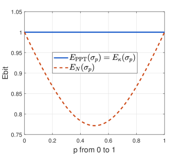
Figure 1: $\kappa$-entanglement and logarithmic negativity of $\sigma_{p}$

Example 2: Let us consider the following class of rank-three two-qutrit states:

$$\omega_{p}=\frac{p}{2}|u_{1}\rangle\!\langle u_{1}|+\frac{1-p}{2}|u_{2}\rangle\!\langle u_{2}|+\frac{1}{2}|u_{3}\rangle\!\langle u_{3}|,$$ (S145)

with $|u_{1}\rangle=|000\rangle$, $|u_{2}\rangle={1}/{\sqrt{2}}(|02\rangle+|20\rangle)$, and $|u_{3}\rangle={1}/{\sqrt{2}}(|12\rangle+|21\rangle)$. The numerical comparison is presented in Figure 2.

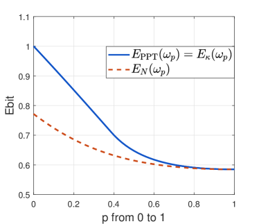
Figure 2: $\kappa$-entanglement and logarithmic negativity of $\omega_{p}$

Example 3: Let us consider the following class of full-rank two-qutrit states:

$$\tau_{p}=\frac{3p}{4}|w_{1}\rangle\!\langle w_{1}|+\frac{3(1-p)}{4}|w_{2}\rangle\!\langle w_{2}|+\frac{I/9}{4},$$ (S146)

with $|w_{1}\rangle={1}/{\sqrt{3}}(|00\rangle+|12\rangle+|21\rangle)$, $|w_{2}\rangle={1}/{\sqrt{2}}(|02\rangle+|20\rangle)$. The numerical comparison is presented in Figure 3.

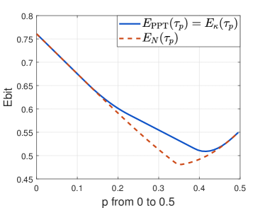
Figure 3: $\kappa$-entanglement and logarithmic negativity of $\tau_{p}$

Appendix G Equality of $E_{\kappa}$ and $E^{\text{dual}}_{\kappa}$ for states acting on separable Hilbert spaces

In this section, we prove that

$$E_{\kappa}(\rho_{AB})=E_{\kappa}^{\text{dual}}(\rho_{AB}),$$ (S147)

for a state $\rho_{AB}$ acting on a separable Hilbert space. To begin with, let us recall that the following inequality always holds from weak duality

$$E_{\kappa}(\rho_{AB})\geq E_{\kappa}^{\text{dual}}(\rho_{AB}).$$ (S148)

So our goal is to prove the opposite inequality. We suppose throughout that $E_{\kappa}^{\text{dual}}(\rho_{AB})<\infty$. Otherwise, the desired equality in (S147) is trivially true. We also suppose that $\rho_{AB}$ has full support. Otherwise, it is finite-dimensional and the desired equality in (S147) is trivially true, or it has only finitely many zero entries, in which case it is isomorphic to a state with full support.

To this end, consider sequences $\{\Pi_{A}^{k}\}_{k}$ and $\{\Pi_{B}^{k}\}_{k}$ of projectors weakly converging to the identities ${\mathds{1}}_{A}$ and ${\mathds{1}}_{B}$ and such that $\Pi_{A}^{k}\leq\Pi_{A}^{k^{\prime}}$ and $\Pi_{B}^{k}\leq\Pi_{B}^{k^{\prime}}$ for $k^{\prime}\geq k$. Furthermore, we suppose that $[\Pi_{B}^{k}]^{T_{B}}=\Pi_{B}^{k}$ for all $k$. Then define

$$\rho_{AB}^{k}\coloneqq\left(\Pi_{A}^{k}\otimes\Pi_{B}^{k}\right)\rho_{AB}\left(\Pi_{A}^{k}\otimes\Pi_{B}^{k}\right).$$ (S149)

It follows that Dell’Antonio (1967)

$$\lim_{k\rightarrow\infty}\left\|\rho_{AB}-\rho_{AB}^{k}\right\|_{1}=0.$$ (S150)

We now prove that

$$E_{\kappa}^{\text{dual}}(\rho_{AB})\geq E_{\kappa}^{\text{dual}}(\rho_{AB}^{k})$$ (S151)

for all $k$. Let $A^{k}$ and $B^{k}$ denote the subspaces onto which $\Pi_{A}^{k}$ and $\Pi_{B}^{k}$ project. Let $V_{A^{k}B^{k}}^{k}$ and $W_{A^{k}B^{k}}^{k}$ be arbitrary operators satisfying $V_{AB}^{k}+W_{AB}^{k}\leq{\mathds{1}}_{A^{k}B^{k}}=\left(\Pi_{A}^{k}\otimes\Pi_{B}^{k}\right)$, $[V_{A^{k}B^{k}}^{k}]^{T_{B}},[W_{A^{k}B^{k}}^{k}]^{T_{B}}\geq 0$. Set

$$\overline{V}_{AB}^{k} \coloneqq\left(\Pi_{A}^{k}\otimes\Pi_{B}^{k}\right)V_{A^{k}B^{k}}^{k}\left(\Pi_{A}^{k}\otimes\Pi_{B}^{k}\right),$$ (S152)

$$\overline{W}_{AB}^{k} \coloneqq\left(\Pi_{A}^{k}\otimes\Pi_{B}^{k}\right)W_{A^{k}B^{k}}^{k}\left(\Pi_{A}^{k}\otimes\Pi_{B}^{k}\right),$$ (S153)

and note that

$$\overline{V}_{AB}^{k}+\overline{W}_{AB}^{k} \leq{\mathds{1}}_{AB},$$ (S154)

$$[\overline{V}_{AB}^{k}]^{T_{B}},[\overline{W}_{AB}^{k}]^{T_{B}} \geq 0.$$ (S155)

Then

$$\operatorname{Tr}\rho_{AB}^{k}(V_{A^{k}B^{k}}^{k}-W_{A^{k}B^{k}}^{k}) =\operatorname{Tr}\left(\Pi_{A}^{k}\otimes\Pi_{B}^{k}\right)\rho_{AB}\left(\Pi_{A}^{k}\otimes\Pi_{B}^{k}\right)(V_{A^{k}B^{k}}^{k}-W_{A^{k}B^{k}}^{k})$$ (S156)

$$=\operatorname{Tr}\rho_{AB}\left(\Pi_{A}^{k}\otimes\Pi_{B}^{k}\right)(V_{A^{k}B^{k}}^{k}-W_{A^{k}B^{k}}^{k})\left(\Pi_{A}^{k}\otimes\Pi_{B}^{k}\right)$$ (S157)

$$=\operatorname{Tr}\rho_{AB}(\overline{V}_{AB}^{k}-\overline{W}_{AB}^{k})$$ (S158)

$$\leq E_{\kappa}^{\text{dual}}(\rho_{AB}).$$ (S159)

Since the inequality holds for arbitrary $V_{A^{k}B^{k}}^{k}$ and $W_{A^{k}B^{k}}^{k}$ satisfying the conditions above, we conclude the inequality in (S151).

Thus, we conclude that

$$E_{\kappa}^{\text{dual}}(\rho_{AB})\geq\limsup_{k\rightarrow\infty}E_{\kappa}^{\text{dual}}(\rho_{AB}^{k}).$$ (S160)

Now let us suppose that $E_{\kappa}^{\text{dual}}(\rho_{AB})<\infty$. Then for all $V_{AB}$ and $W_{AB}$ satisfying $V_{AB}+W_{AB}\leq{\mathds{1}}_{AB}$, $[V_{AB}]^{T_{B}},[W_{AB}]^{T_{B}}\geq 0$, as well as $\operatorname{Tr}\rho_{AB}(V_{AB}-W_{AB})\geq 0$, we have that

$$\operatorname{Tr}\rho_{AB}(V_{AB}-W_{AB})<\infty.$$ (S161)

Since $\rho_{AB}$ has full support, this means that

$$\left\|V_{AB}-W_{AB}\right\|_{\infty}<\infty.$$ (S162)

Considering that from Hölder’s inequality

$$\left|\operatorname{Tr}(\rho_{AB}-\rho_{AB}^{k})(V_{AB}-W_{AB})\right|\leq\left\|\rho_{AB}-\rho_{AB}^{k}\right\|_{1}\left\|V_{AB}-W_{AB}\right\|_{\infty},$$ (S163)

and setting

$$V_{AB}^{k} \coloneqq\left(\Pi_{A}^{k}\otimes\Pi_{B}^{k}\right)V_{AB}\left(\Pi_{A}^{k}\otimes\Pi_{B}^{k}\right),$$ (S164)

$$W_{AB}^{k} \coloneqq\left(\Pi_{A}^{k}\otimes\Pi_{B}^{k}\right)W_{AB}\left(\Pi_{A}^{k}\otimes\Pi_{B}^{k}\right),$$ (S165)

we conclude that

$$\operatorname{Tr}\rho_{AB}(V_{AB}-W_{AB}) \leq\liminf_{k\rightarrow\infty}\operatorname{Tr}\rho_{AB}^{k}(V_{AB}-W_{AB})$$ (S166)

$$=\liminf_{k\rightarrow\infty}\operatorname{Tr}\rho_{AB}^{k}(V_{AB}^{k}-W_{AB}^{k})$$ (S167)

$$\leq\liminf_{k\rightarrow\infty}\sup_{V^{k},W^{k}}\operatorname{Tr}\rho_{AB}^{k}(V_{AB}^{k}-W_{AB}^{k})$$ (S168)

$$=\liminf_{k\rightarrow\infty}E_{\kappa}^{\text{dual}}(\rho_{AB}^{k}).$$ (S169)

Since the inequality holds for arbitrary $V_{AB}$ and $W_{AB}$ satisfying the above conditions, we conclude that

$$E_{\kappa}^{\text{dual}}(\rho_{AB})\leq\liminf_{k\rightarrow\infty}E_{\kappa}^{\text{dual}}(\rho_{AB}^{k}).$$ (S170)

Putting together (S160) and (S170), we conclude that

$$E_{\kappa}^{\text{dual}}(\rho_{AB})=\lim_{k\rightarrow\infty}E_{\kappa}^{\text{dual}}(\rho_{AB}^{k}).$$ (S171)

From strong duality for the finite-dimensional case, we have for all $k$ that

$$E_{\kappa}^{\text{dual}}(\rho_{AB}^{k})=E_{\kappa}(\rho_{AB}^{k}),$$ (S172)

and thus that

$$\lim_{k\rightarrow\infty}E_{\kappa}^{\text{dual}}(\rho_{AB}^{k})=\lim_{k\rightarrow\infty}E_{\kappa}(\rho_{AB}^{k}).$$ (S173)

It thus remains to prove that

$$\lim_{k\rightarrow\infty}E_{\kappa}(\rho_{AB}^{k})=E_{\kappa}(\rho_{AB}).$$ (S174)

We first prove that

$$E_{\kappa}(\rho_{AB})\geq\limsup_{k\rightarrow\infty}E_{\kappa}(\rho_{AB}^{k}).$$ (S175)

Let $S_{AB}$ be an arbitrary operator satisfying

$$S_{AB}\geq 0,\qquad-S_{AB}^{T_{B}}\leq\rho_{AB}^{T_{B}}\leq S_{AB}^{T_{B}}.$$ (S176)

Then, defining $S_{AB}^{k}=\left(\Pi_{A}^{k}\otimes\Pi_{B}^{k}\right)S_{AB}\left(\Pi_{A}^{k}\otimes\Pi_{B}^{k}\right)$, we have that

$$S_{AB}^{k}\geq 0,\qquad-[S_{AB}^{k}]^{T_{B}}\leq[\rho_{AB}^{k}]^{T_{B}}\leq[S_{AB}^{k}]^{T_{B}}.$$ (S177)

Then

$$\log_{2}\operatorname{Tr}S_{AB}\geq\log_{2}\operatorname{Tr}S_{AB}^{k}\geq E_{\kappa}(\rho_{AB}^{k}).$$ (S178)

Since the inequality holds for all $S_{AB}$ satisfying (S176), we conclude that

$$E_{\kappa}(\rho_{AB})\geq E_{\kappa}(\rho_{AB}^{k})$$ (S179)

for all $k$, and thus (S175) holds.

The rest of the proof follows Furrer et al. (2011) closely. Since the condition $\Pi_{A}^{k}\leq\Pi_{A}^{k^{\prime}}$ and $\Pi_{B}^{k}\leq\Pi_{B}^{k^{\prime}}$ for $k^{\prime}\geq k$ holds, in fact the same sequence of steps as above allows for concluding that

$$E_{\kappa}(\rho_{AB}^{k^{\prime}})\geq E_{\kappa}(\rho_{AB}^{k}),$$ (S180)

meaning that the sequence is monotone non-decreasing with $k$. Thus, we can define

$$\mu\coloneqq\lim_{k\rightarrow\infty}E_{\kappa}(\rho_{AB}^{k})\in\mathbb{R}^{+},$$ (S181)

and note from the above that

$$\mu\leq E_{\kappa}(\rho_{AB}).$$ (S182)

For each $k$, let $S_{AB}^{k}$ denote an optimal operator such that $E_{\kappa}(\rho_{AB}^{k})=\log_{2}\operatorname{Tr}S_{AB}^{k}$. From the fact that $S_{AB}^{k}\geq 0$, and $\operatorname{Tr}S_{AB}^{k}\leq 2^{\mu}$, we conclude that $\{S_{AB}^{k}\}_{k}$ is a bounded sequence in the trace class operators. Since the trace class operators form the dual space of the compact operators $\mathcal{K}(\mathcal{H}_{AB})$ Reed and Simon (1978), we can apply the Banach–Alaoglu theorem Reed and Simon (1978) to find a subsequence $\{S_{AB}^{k}\}_{k\in\Gamma}$ with a weak^∗ limit $\widetilde{S}_{AB}$ in the trace class operators such that $\widetilde{S}_{AB}\geq 0$ and $\operatorname{Tr}[\widetilde{S}_{AB}]\leq 2^{\mu}$. Furthermore, the sequences $[\rho_{AB}^{k}]^{T_{B}}+[S_{AB}^{k}]^{T_{B}}$ and $[S_{AB}^{k}]^{T_{B}}-[\rho_{AB}^{k}]^{T_{B}}$ converge in the weak operator topology to $\rho_{AB}^{T_{B}}+\widetilde{S}_{AB}^{T_{B}}$ and $\widetilde{S}_{AB}^{T_{B}}-\rho_{AB}^{T_{B}}$, respectively, and we can then conclude that $\rho_{AB}^{T_{B}}+\widetilde{S}_{AB}^{T_{B}},\widetilde{S}_{AB}^{T_{B}}-\rho_{AB}^{T_{B}}\geq 0$. But this means that

$$E_{\kappa}(\rho_{AB})\leq\log_{2}\operatorname{Tr}\widetilde{S}_{AB}\leq\mu,$$ (S183)

which implies that

$$E_{\kappa}(\rho_{AB})\leq\liminf_{k\rightarrow\infty}E_{\kappa}(\rho_{AB}^{k}).$$ (S184)

Putting together (S175) and (S184), we conclude that

$$E_{\kappa}(\rho_{AB})=\lim_{k\rightarrow\infty}E_{\kappa}(\rho_{AB}^{k}).$$ (S185)

Finally, putting together (S171), (S173), and (S185), we conclude (S147).

References

Schrödinger (1935)Erwin Schrödinger, “Discussion of probability relations between separated systems,” Proceedings of the
Cambridge Philosophical Society 31, 555–563 (1935).
Einstein et al. (1935)Albert Einstein, Boris Podolsky, and Nathan Rosen, “Can
quantum-mechanical description of physical reality be considered complete?” Physical Review 47, 777–780 (1935).
Bell (1964)John Stewart Bell, “On
the Einstein-Podolsky-Rosen paradox,” Physics 1, 195–200 (1964).
Aspect et al. (1981)Alain Aspect, Philippe Grangier, and Gérard Roger, “Experimental
tests of realistic local theories via Bell’s theorem,” Physical Review Letters 47, 460–463 (1981).
Hensen et al. (2015)B. Hensen, H. Bernien,
A. E. Dreau, A. Reiserer, N. Kalb, M. S. Blok, J. Ruitenberg, R. F. L. Vermeulen, R. N. Schouten, C. Abellan, W. Amaya,
V. Pruneri, M. W. Mitchell, M. Markham, D. J. Twitchen, D. Elkouss, S. Wehner, T. H. Taminiau, and R. Hanson, “Loophole-free Bell inequality violation using electron spins separated by
1.3 kilometres,” Nature 526, 682–686 (2015), arXiv:1508.05949.
Giustina et al. (2015)Marissa Giustina, Marijn A. M. Versteegh, Sören Wengerowsky, Johannes Handsteiner, Armin Hochrainer, Kevin Phelan, Fabian Steinlechner, Johannes Kofler, Jan-Åke Larsson, Carlos Abellán, Waldimar Amaya, Valerio Pruneri, Morgan W. Mitchell, Jörn Beyer, Thomas Gerrits,
Adriana E. Lita, Lynden K. Shalm, Sae Woo Nam, Thomas Scheidl, Rupert Ursin, Bernhard Wittmann, and Anton Zeilinger, “Significant-loophole-free test of Bell’s
theorem with entangled photons,” Physical Review Letters 115, 250401 (2015), arXiv:1511.03190.
Shalm et al. (2015)Lynden K. Shalm, Evan Meyer-Scott, Bradley G. Christensen, Peter Bierhorst, Michael A. Wayne, Martin J. Stevens, Thomas Gerrits, Scott Glancy,
Deny R. Hamel, Michael S. Allman, Kevin J. Coakley, Shellee D. Dyer, Carson Hodge, Adriana E. Lita, Varun B. Verma, Camilla Lambrocco, Edward Tortorici, Alan L. Migdall, Yanbao Zhang, Daniel R. Kumor, William H. Farr, Francesco Marsili, Matthew D. Shaw, Jeffrey A. Stern, Carlos Abellán, Waldimar Amaya, Valerio Pruneri, Thomas Jennewein, Morgan W. Mitchell, Paul G. Kwiat, Joshua C. Bienfang, Richard P. Mirin, Emanuel Knill, and Sae Woo Nam, “Strong loophole-free test of local realism,” Physical Review Letters 115, 250402 (2015), arXiv:1511.03189.
Nielsen and Chuang (2000)Michael A. Nielsen and Isaac L. Chuang, Quantum
Computation and Quantum Information (Cambridge
University Press, 2000).
Wilde (2017)Mark M. Wilde, Quantum Information
Theory, 2nd ed. (Cambridge
University Press, 2017) arXiv:1106.1445.
Bennett et al. (1993)Charles H. Bennett, Gilles Brassard, Claude Crépeau, Richard Jozsa, Asher Peres, and William K. Wootters, “Teleporting an
unknown quantum state via dual classical and Einstein-Podolsky-Rosen
channels,” Physical Review Letters 70, 1895–1899 (1993).
Bennett and Wiesner (1992)Charles H. Bennett and Stephen J. Wiesner, “Communication via one- and two-particle operators on
Einstein-Podolsky-Rosen states,” Physical Review Letters 69, 2881–2884 (1992).
Bennett and Brassard (1984)Charles H. Bennett and Gilles Brassard, “Quantum cryptography: Public key distribution and coin tossing,” in Proceedings of IEEE International
Conference on Computers Systems and Signal Processing (Bangalore, India, 1984) pp. 175–179.
Bennett et al. (1996a)Charles H. Bennett, David P. DiVincenzo, John A. Smolin, and William K. Wootters, “Mixed-state entanglement and quantum error correction,” Physical Review A 54, 3824–3851 (1996a), arXiv:quant-ph/9604024.
Terhal and Horodecki (2000)Barbara M. Terhal and Paweł Horodecki, “Schmidt number for density matrices,” Physical Review A 61, 040301 (2000), arXiv:quant-ph/9911117.
Bennett et al. (1996b)Charles H. Bennett, Herbert J. Bernstein, Sandu Popescu, and Benjamin Schumacher, “Concentrating partial entanglement by local operations,” Physical Review A 53, 2046–2052 (1996b), arXiv:quant-ph/9511030.
Vedral and Plenio (1998)Vlatko Vedral and Martin B. Plenio, “Entanglement
measures and purification procedures,” Physical Review A 57, 1619–1633 (1998), arXiv:quant-ph/9707035.
Rains (2001)Eric M. Rains, “A semidefinite
program for distillable entanglement,” IEEE Transactions on Information Theory 47, 2921–2933 (2001), arXiv:quant-ph/0008047.
Vidal and Werner (2002)Guifre Vidal and Reinhard F. Werner, “Computable
measure of entanglement,” Physical Review A 65, 032314 (2002), arXiv:quant-ph/0102117.
Christandl and Winter (2004)Matthias Christandl and Andreas Winter, ““Squashed entanglement”: an additive entanglement measure,” Journal of Mathematical
Physics 45, 829–840
(2004), arXiv:quant-ph/0308088.
Plenio (2005)Martin B. Plenio, “Logarithmic negativity: A full entanglement monotone that is not convex,” Physical Review Letters 95, 090503 (2005), arXiv:quant-ph/0505071.
Plenio and Virmani (2007)Martin B. Plenio and Shashank S. Virmani, “An
introduction to entanglement measures,” Quantum Information and Computation 7, 1–51 (2007), arXiv:quant-ph/0504163.
Horodecki et al. (2009)Ryszard Horodecki, Paweł Horodecki, Michał Horodecki, and Karol Horodecki, “Quantum
entanglement,” Reviews of Modern Physics 81, 865–942 (2009), arXiv:quant-ph/0702225.
Wang and Duan (2016)Xin Wang and Runyao Duan, “An improved
semidefinite programming upper bound on distillable entanglement,” Physical Review
A 94, 050301 (2016), arXiv:1601.07940.
Wang and Duan (2017)Xin Wang and Runyao Duan, “Irreversibility of
asymptotic entanglement manipulation under quantum operations completely
preserving positivity of partial transpose,” Physical Review Letters 119, 180506 (2017), arXiv:1606.09421.
Huang (2014)Yichen Huang, “Computing quantum
discord is NP-complete,” New Journal of Physics 16, 33027 (2014).
Chitambar et al. (2014)Eric Chitambar, Debbie Leung, Laura Mančinska, Maris Ozols, and Andreas Winter, “Everything you
always wanted to know about LOCC (but were afraid to ask),” Communications in Mathematical Physics 328, 303–326 (2014), arXiv:1210.4583.
Chitambar et al. (2017)Eric Chitambar, Julio I. de Vicente, Mark W. Girard, and Gilad Gour, “Entanglement
manipulation and distillability beyond LOCC,” (2017), arXiv:1711.03835.
Eggeling et al. (2001)Tilo Eggeling, Karl Gerd H. Vollbrecht, Reinhard F. Werner, and Michael M. Wolf, “Distillability via
protocols respecting the positivity of partial transpose,” Physical Review Letters 87, 257902 (2001), arXiv:quant-ph/0104095.
Audenaert et al. (2003)Koenraad Audenaert, Martin B. Plenio, and Jens Eisert, “Entanglement cost under positive-partial-transpose-preserving operations,” Physical Review Letters 90, 027901 (2003), arXiv:quant-ph/0207146.
Horodecki et al. (2002)Michał Horodecki, Jonathan Oppenheim, and Ryszard Horodecki, “Are the laws of entanglement theory thermodynamical?” Physical Review Letters 89, 240403 (2002), arXiv:quant-ph/0207177.
Matthews and Winter (2008)William Matthews and Andreas Winter, “Pure-state
transformations and catalysis under operations that completely preserve
positivity of partial transpose,” Physical Review A 78, 012317 (2008), arXiv:0801.4322.
Boyd and Vandenberghe (2004)Stephen Boyd and Lieven Vandenberghe, Convex
Optimization (Cambridge University Press, The Edinburgh Building, Cambridge, CB2 8RU, UK, 2004).
Khachiyan (1980)Leonid G. Khachiyan, “Polynomial algorithms in linear programming,” USSR Computational Mathematics and
Mathematical Physics 20, 53–72 (1980).
Arora et al. (2005)Sanjeev Arora, Elad Hazan,
and Satyen Kale, “Fast algorithms for
approximate semidefinite programming using the multiplicative weights update
method,” in 46th Annual IEEE
Symposium on Foundations of Computer Science (2005) pp. 339–348.
Arora et al. (2012)Sanjeev Arora, Elad Hazan, and Satyen Kale, “The multiplicative weights
update method: a meta-algorithm and applications,” Theory
of Computing 8, 121–164
(2012).
Lee et al. (2015)Yin Tat Lee, Aaron Sidford, and Sam Chiu Wai Wong, “A faster cutting plane
method and its implications for combinatorial and convex optimization,” in IEEE 56th Annual Symposium
on the Foundations of Computer Science (2015) pp. 1049–1065, arXiv:1508.04874.
Terhal (2004)Barbara M. Terhal, “Is
entanglement monogamous?” IBM Journal of Research and Development 48, 71–78 (2004), arXiv:quant-ph/0307120.
Wang and Wilde (2020)Xin Wang and Mark M. Wilde, “Supplementary
Material for ‘Cost of quantum entanglement simplified’,” (2020).
Hayashi (2006)Masahito Hayashi, Quantum
Information: An Introduction (Springer, 2006).
Yue and Chitambar (2018)Qiuling Yue and Eric Chitambar, “The
zero-error entanglement cost is highly non-additive,” (2018), arXiv:1808.10516.
Horodecki and Horodecki (1999)Michał Horodecki and Paweł Horodecki, “Reduction criterion of separability and limits for a class
of distillation protocols,” Physical Review A 59, 4206–4216 (1999), arXiv:quant-ph/9708015.
Watrous (2018)John Watrous, The Theory of Quantum
Information (Cambridge University Press, 2018).
Ishizaka (2004)Satoshi Ishizaka, “Binegativity
and geometry of entangled states in two qubits,” Physical Review A 69, 020301 (2004), arXiv:quant-ph/0308056.
Coffman et al. (2000)Valerie Coffman, Joydip Kundu,
and William K. Wootters, “Distributed
entanglement,” Physical Review A 61, 052306 (2000), arXiv:quant-ph/9907047.
Koashi and Winter (2004)Masato Koashi and Andreas Winter, “Monogamy of
quantum entanglement and other correlations,” Physical Review A 69, 022309 (2004), arXiv:quant-ph/0310037.
Reed and Simon (1978)M. Reed and B. Simon, Methods of Modern Mathematical
Physics, Vol. I: Functional Analysis (Academic Press, New York, 1978).
Gour and Scandolo (2019)Gilad Gour and Carlo Maria Scandolo, “The
entanglement of a bipartite channel,” (2019), arXiv:1907.02552v3.
Wang and Wilde (2018)Xin Wang and Mark M. Wilde, “Exact
entanglement cost of quantum states and channels under PPT-preserving
operations,” (2018), arXiv:1809.09592v1.
Brandao (2005)Fernando G. S. L. Brandao, “Quantifying entanglement with witness operators,” Physical Review A 72, 022310 (2005), arXiv:quant-ph/0503152.
Werner (1989)Reinhard F. Werner, “Quantum states with Einstein-Podolsky-Rosen correlations admitting a
hidden-variable model,” Physical Review A 40, 4277–4281 (1989).
Gurvits (2003)Leonid Gurvits, “Classical
deterministic complexity of Edmonds’ problem and quantum entanglement,” in Proceedings of the
thirty-fifth annual ACM symposium on Theory of computing (2003) pp. 10–19, arXiv:quant-ph/0303055.
Gharibian (2010)Sevag Gharibian, “Strong
NP-hardness of the quantum separability problem,” Quantum Information and
Computation 10, 343–360
(2010), arXiv:0810.4507.
Horodecki et al. (1996)Michał Horodecki, Paweł Horodecki, and Ryszard Horodecki, “Separability of mixed states: necessary and sufficient conditions,” Physics Letters A 223, 1–8 (1996), arXiv:quant-ph/9605038.
Horodecki et al. (1998)Michał Horodecki, Paweł Horodecki, and Ryszard Horodecki, “Mixed-state entanglement and distillation: Is there a “bound” entanglement
in nature?” Physical Review Letters 80, 5239–5242 (1998), arXiv:quant-ph/9801069.
Vandenberghe and Boyd (1996)Lieven Vandenberghe and Stephen Boyd, “Semidefinite Programming,” SIAM Review 38, 49–95 (1996).
Fletcher et al. (2007)Andrew S. Fletcher, Peter W. Shor, and Moe Z. Win, “Optimum quantum error recovery using semidefinite programming,” Physical Review A 75, 012338 (2007), arXiv:quant-ph/0606035.
Horodecki (2005)Michal Horodecki, “Simplifying
monotonicity conditions for entanglement measures,” Open Systems & Information
Dynamics 12, 231–237
(2005), arXiv:quant-ph/0412210.
Gour and Guo (2018)Gilad Gour and Yu Guo, “Monogamy of entanglement
without inequalities,” Quantum 2, 81 (2018), arXiv:1710.03295.
Horodecki et al. (2000)Michał Horodecki, Paweł Horodecki, and Ryszard Horodecki, “Asymptotic manipulations of entanglement can exhibit genuine
irreversibility,” Physical Review Letters 84, 4260–4263 (2000), arXiv:quant-ph/9912076.
Shor et al. (2001)Peter W. Shor, John A. Smolin, and Barbara M. Terhal, “Nonadditivity of bipartite distillable entanglement follows from a
conjecture on bound entangled Werner states,” Physical Review Letters 86, 2681–2684 (2001), arXiv:quant-ph/0010054.
Shor et al. (2003)Peter W. Shor, John A. Smolin, and Ashish V. Thapliyal, “Superactivation of bound entanglement,” Physical Review Letters 90, 107901 (2003), arXiv:quant-ph/0005117.