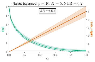
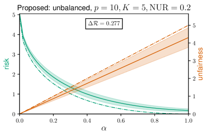
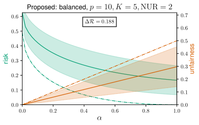
\startlocaldefs\endlocaldefs

and

A minimax framework for quantifying risk-fairness trade-off in regression

Evgenii Chzhenlabel=e1]evgenii.chzhen@universite-paris-saclay.fr [    Nicolas Schreuderlabel=e2]nicolas.schreuder@ensae.fr [ Université Paris-Saclay, CNRS, Laboratoire de mathématiques d’Orsay
Università di Genova, MaLGa, DIBRIS
Institut Polytechnique de Paris, ENSAE, CREST
Abstract

We propose a theoretical framework for the problem of learning a real-valued function which meets fairness requirements. This framework is built upon the notion of α𝛼\alpha-relative (fairness) improvement of the regression function which we introduce using the theory of optimal transport. Setting α=0𝛼0\alpha=0 corresponds to the regression problem under the Demographic Parity constraint, while α=1𝛼1\alpha=1 corresponds to the classical regression problem without any constraints. For α(0,1)𝛼01\alpha\in(0,1) the proposed framework allows to continuously interpolate between these two extreme cases and to study partially fair predictors. Within this framework we precisely quantify the cost in risk induced by the introduction of the fairness constraint. We put forward a statistical minimax setup and derive a general problem-dependent lower bound on the risk of any estimator satisfying α𝛼\alpha-relative improvement constraint. We illustrate our framework on a model of linear regression with Gaussian design and systematic group-dependent bias, deriving matching (up to absolute constants) upper and lower bounds on the minimax risk under the introduced constraint. We provide a general post-processing strategy which enjoys fairness, risk guarantees and can be applied on top of any black-box algorithm. Finally, we perform a simulation study of the linear model and numerical experiments of benchmark data, validating our theoretical contributions.

Algorithmic fairness,
risk-fairness trade-off,
regressions,
Demographic Parity,
least-squares,
optimal transport,
minimax analysis,
statistical learning,
keywords:

1 Introduction

Data driven algorithms are deployed in almost all areas of modern daily life and it becomes increasingly more important to adequately address the fundamental issue of historical biases present in the data (Barocas, Hardt and Narayanan, 2019). The goal of algorithmic fairness is to bridge the gap between the statistical theory of decision making and the understanding of justice, equality, and diversity. The literature on fairness is broad and its volume increases day by day, we refer the reader to (Mehrabi et al., 2019, Barocas, Hardt and Narayanan, 2019) for a general introduction on the subject and to (Oneto and Chiappa, 2020, del Barrio, Gordaliza and Loubes, 2020) for reviews of the most recent theoretical advances.

Basically, the mathematical definitions of fairness can be divided into two groups (Dwork et al., 2012): individual fairness and group fairness. The former notion reflects the principle that similar individuals must be treated similarly, which translates into Lipschitz type constraints on possible prediction rules. The latter defines fairness on population level via (conditional) statistical independence of a prediction from a sensitive attribute (e.g., gender, ethnicity). A popular formalization of such notion is through the Demographic Parity constraint, initially introduced in the context of binary classification (Calders, Kamiran and Pechenizkiy, 2009). Despite of some limitations (Hardt, Price and Srebro, 2016), the concept of Demographic Parity is natural and suitable for a range of applied problems (Köeppen, Yoshida and Ohnishi, 2014, Zink and Rose, 2019).

In this work we study the regression problem of learning a real-valued prediction function, which complies with an approximate notion of Demographic Parity while minimizing expected squared loss.

Unlike its classification counterpart, the problem of fair regression has received far less attention in the literature. However, as argued by Agarwal, Dudik and Wu (2019), classifiers only provide binary decisions, while in practice final decisions are taken by humans based on predictions from the machine. In this case a continuous prediction is more informative than a binary one and justifies the need for studying fairness in the regression framework.

Notation. For any univariate probability measure μ𝜇\mu we denote by Fμsubscript𝐹𝜇F_{\mu} (resp. Fμ1superscriptsubscript𝐹𝜇1F_{\mu}^{-1}) the cumulative distribution function (resp. the quantile function) of μ𝜇\mu. For two random variables U𝑈U and V𝑉V we denote by Law(UV=v)Lawconditional𝑈𝑉𝑣\operatorname{Law}(U\mid V{=}v) the conditional distribution of the random variable UV=vconditional𝑈𝑉𝑣U\mid V{=}v and we write U=dVsuperscript𝑑𝑈𝑉U\stackrel{{\scriptstyle d}}{{=}}V to denote their equality in distribution. For any integer K1𝐾1K\geq 1, we denote by ΔK1superscriptΔ𝐾1\Delta^{K-1} the probability simplex in Ksuperscript𝐾\mathbb{R}^{K} and we write [K]={1,,K}delimited-[]𝐾1𝐾[K]=\{1,\dots,K\}. For any a,b𝑎𝑏a,b\in\mathbb{R} we denote by ab𝑎𝑏a\vee b (resp. ab𝑎𝑏a\wedge b) the maximum (resp. the minimum) between a,b𝑎𝑏a,b. We denote by 𝒫2(d)subscript𝒫2superscript𝑑\mathcal{P}_{2}(\mathbb{R}^{d}) the space of probability measures on dsuperscript𝑑\mathbb{R}^{d} with finite second-order moment.

2 Problem statement and contributions

We study the regression problem when a sensitive attribute is available. The statistician observes triplets (𝑿1,S1,Y1),,(𝑿n,Sn,Yn)p×[K]×subscript𝑿1subscript𝑆1subscript𝑌1subscript𝑿𝑛subscript𝑆𝑛subscript𝑌𝑛superscript𝑝delimited-[]𝐾(\boldsymbol{X}_{1},S_{1},Y_{1}),\ldots,(\boldsymbol{X}_{n},S_{n},Y_{n})\in\mathbb{R}^{p}\times[K]\times\mathbb{R}, which are connected by the following regression-type relation

Yi=f(𝑿i,Si)+ξi,i[n],formulae-sequencesubscript𝑌𝑖superscript𝑓subscript𝑿𝑖subscript𝑆𝑖subscript𝜉𝑖𝑖delimited-[]𝑛\displaystyle Y_{i}=f^{*}(\boldsymbol{X}_{i},S_{i})+\xi_{i}\enspace,\qquad i\in[n]\enspace, (1)

where ξisubscript𝜉𝑖\xi_{i}\in\mathbb{R} is such that 𝐄[ξi𝑿i]=0𝐄delimited-[]conditionalsubscript𝜉𝑖subscript𝑿𝑖0\mathbf{E}[\xi_{i}\mid\boldsymbol{X}_{i}]=0 and f:p×[K]:superscript𝑓superscript𝑝delimited-[]𝐾f^{*}:\mathbb{R}^{p}\times[K]\to\mathbb{R} is the regression function. Here for each i[n]𝑖delimited-[]𝑛i\in[n], 𝑿isubscript𝑿𝑖\boldsymbol{X}_{i} is a feature vector taking values in psuperscript𝑝\mathbb{R}^{p}, Sisubscript𝑆𝑖S_{i} is a sensitive attribute taking values in [K]delimited-[]𝐾[K], and Yisubscript𝑌𝑖Y_{i} is a real-valued dependent variable. A prediction is any measurable function of the form f:p×[K]:𝑓superscript𝑝delimited-[]𝐾f:\mathbb{R}^{p}\times[K]\to\mathbb{R}. We define the risk of a prediction function f𝑓f via the 2subscript2\ell_{2} distance111The extension to qsubscript𝑞\ell_{q} losses is provided in Appendix G. to the regression function fsuperscript𝑓f^{*} as

(f):=ff22:=s=1Kws𝔼[(f(𝑿,S)f(𝑿,S))2S=s],assign𝑓superscriptsubscriptnorm𝑓superscript𝑓22assignsuperscriptsubscript𝑠1𝐾subscript𝑤𝑠𝔼delimited-[]conditionalsuperscript𝑓𝑿𝑆superscript𝑓𝑿𝑆2𝑆𝑠\displaystyle\mathcal{R}(f)\vcentcolon=\|f-f^{*}\|_{2}^{2}\vcentcolon=\sum_{s=1}^{K}w_{s}\mathbb{E}\left[(f(\boldsymbol{X},S)-f^{*}(\boldsymbol{X},S))^{2}\mid S=s\right]\enspace, (Risk measure)

where 𝔼[S=s]\mathbb{E}[\cdot\mid S{=}s] is the expectation w.r.t. the distribution of the features 𝑿𝑿\boldsymbol{X} in the group S=s𝑆𝑠S=s and 𝒘=(w1,,wK)ΔK1𝒘superscriptsubscript𝑤1subscript𝑤𝐾topsuperscriptΔ𝐾1\boldsymbol{w}=(w_{1},\ldots,w_{K})^{\top}\in\Delta^{K-1} is a probability vector, which weights the group-wise risks.

For any s[K]𝑠delimited-[]𝐾s\in[K] define νssubscriptsuperscript𝜈𝑠\nu^{*}_{s} as Law(f(𝑿,S)S=s)Lawconditionalsuperscript𝑓𝑿𝑆𝑆𝑠\operatorname{Law}(f^{*}(\boldsymbol{X},S)\mid S{=}s) – the distribution of the optimal prediction inside the group S=s𝑆𝑠S=s. Throughout this work we make the following assumption on those measures, which is, for instance, satisfied in linear regression with Gaussian design.

Assumption 2.1.

Measures {νs}s[K]subscriptsubscriptsuperscript𝜈𝑠𝑠delimited-[]𝐾\{\nu^{*}_{s}\}_{s\in[K]} are non-atomic with finite second moments.

2.1 Regression with fairness constraints

Any predictor f𝑓f induces a group-wise distribution of the predicted outcomes Law(f(𝑿,S)S=s)Lawconditional𝑓𝑿𝑆𝑆𝑠\operatorname{Law}(f(\boldsymbol{X},S)\mid S{=}s) for s[K]𝑠delimited-[]𝐾s\in[K]. The high-level idea of group fairness notions is to bound or diminish an eventual discrepancy between these distributions.

We define the unfairness of a predictor f𝑓f as the sum of the weighted distances between {Law(f(𝑿,S)S=s)}s[K]subscriptLawconditional𝑓𝑿𝑆𝑆𝑠𝑠delimited-[]𝐾\{\operatorname{Law}(f(\boldsymbol{X},S)\mid S{=}s)\}_{s\in[K]} and their common barycenter w.r.t. the Wasserstein-2 distance222See Appendix A.1 for a reminder on Wasserstein distances.:

𝒰(f):=minν𝒫2()s=1Kws𝖶22(Law(f(𝑿,S)S=s),ν).assign𝒰𝑓subscript𝜈subscript𝒫2superscriptsubscript𝑠1𝐾subscript𝑤𝑠superscriptsubscript𝖶22Lawconditional𝑓𝑿𝑆𝑆𝑠𝜈\displaystyle\mathcal{U}(f)\vcentcolon=\min_{\nu\in\mathcal{P}_{2}(\mathbb{R})}\sum_{s=1}^{K}w_{s}\mathsf{W}_{2}^{2}\big{(}\operatorname{Law}(f(\boldsymbol{X},S)\mid S{=}s),\,\nu\big{)}\enspace. (Unfairness measure)

In particular, since the Wasserstein-2 distance is a metric on the space probability distributions with finite second-order moment 𝒫2(d)subscript𝒫2superscript𝑑\mathcal{P}_{2}(\mathbb{R}^{d}), a predictor f𝑓f is such that 𝒰(f)=0𝒰𝑓0\mathcal{U}(f)=0 if and only if it satisfies the Demographic Parity (DP) constraint defined as

(f(𝑿,S)S=s\displaystyle\big{(}f(\boldsymbol{X},S)\mid S=s=^d(f(X, S) ∣S = s’),  ∀s, s’ ∈[K]  .UNKNOWNUNKNOWN{} (DP)

Exact DP is not necessarily desirable in practice and it is common in the literature to consider relaxations of this constraint. In this work we introduce the α𝛼\alpha-Relative Improvement (α𝛼\alpha-RI) constraint – a novel DP relaxation based on our unfairness measure. We say that a predictor f𝑓f satisfies the α𝛼\alpha-RI constraint for some α[0,1]𝛼01\alpha\in[0,1] if its unfairness is at most an α𝛼\alpha fraction of the unfairness of the regression function fsuperscript𝑓f^{*}, that is, 𝒰(f)α𝒰(f)𝒰𝑓𝛼𝒰superscript𝑓\mathcal{U}(f)\leq\alpha\,\mathcal{U}(f^{*}). Importantly, the fairness requirement is stated relatively to the unfairness of the regression function fsuperscript𝑓f^{*}, which allows to make a more informed choice of α𝛼\alpha.

Formally, for a fixed α[0,1]𝛼01\alpha\in[0,1], the goal of a statistician in our framework is to build an estimator f^^𝑓\hat{f} using data, which enjoys two guarantees (with high probability)

α-RI guarantee:𝒰(f^)α𝒰(f)andRisk guarantee:(f^)rn,α,f.formulae-sequenceα-RI guarantee:𝒰^𝑓𝛼𝒰superscript𝑓andRisk guarantee:^𝑓subscript𝑟𝑛𝛼superscript𝑓\displaystyle\textbf{$\alpha$-RI guarantee:}\quad\mathcal{U}(\hat{f})\leq\alpha\,\mathcal{U}(f^{*})\qquad\text{and}\qquad\textbf{Risk guarantee:}\quad\mathcal{R}(\hat{f})\leq r_{n,\alpha,f^{*}}\enspace.

The former ensures that f^^𝑓\hat{f} satisfies the α𝛼\alpha-RI constraint. In the latter guarantee we seek the sequence rn,α,fsubscript𝑟𝑛𝛼superscript𝑓r_{n,\alpha,f^{*}} being as small as possible in order to quantify two effects: the introduction of the α𝛼\alpha-RI fairness constraint and the statistical estimation. We note that rn,α,fsubscript𝑟𝑛𝛼superscript𝑓r_{n,\alpha,f^{*}} depends on the sample size n𝑛n, the fairness parameter α𝛼\alpha, as well as the regression function fsuperscript𝑓f^{*} to be estimated, we clarify the reason for this dependency later in the text.

2.2 Contributions

The first natural question that we address is: assuming that the underlying distribution of XSconditional𝑋𝑆X\mid S and the regression function fsuperscript𝑓f^{*} are known, which prediction rule fαsuperscriptsubscript𝑓𝛼f_{\alpha}^{*} minimizes the expected squared loss under the α𝛼\alpha-RI constraint 𝒰(fα)α𝒰(f)𝒰subscriptsuperscript𝑓𝛼𝛼𝒰superscript𝑓\mathcal{U}(f^{*}_{\alpha})\leq\alpha\,\mathcal{U}(f^{*})? To answer this question we shift the discussion to the population level and define a collection {fα}α[0,1]subscriptsubscriptsuperscript𝑓𝛼𝛼01\{f^{*}_{\alpha}\}_{\alpha\in[0,1]} of oracle α𝛼\alpha-RI indexed by the parameter α𝛼\alpha as

fαargmin{(f):𝒰(f)α𝒰(f)},α[0,1].formulae-sequencesubscriptsuperscript𝑓𝛼argmin:𝑓𝒰𝑓𝛼𝒰superscript𝑓for-all𝛼01\displaystyle f^{*}_{\alpha}\in\operatorname*{arg\,min}\left\{\mathcal{R}(f)\,:\,\mathcal{U}(f)\leq\alpha\,\mathcal{U}(f^{*})\right\}\enspace,\qquad\forall\alpha\in[0,1]\enspace. (Oracle α𝛼\alpha-RI)

For α=0𝛼0\alpha=0 the predictor f0subscriptsuperscript𝑓0f^{*}_{0} corresponds to the optimal fair predictor in the sense of DP while for α=1𝛼1\alpha=1 the corresponding predictor f1subscriptsuperscript𝑓1f^{*}_{1} coincides with the regression function fsuperscript𝑓f^{*}. Those two extreme cases have been previously studied but, up to our knowledge, nothing is known about those “partially fair” predictors. Our study of the family {fα}α[0,1]subscriptsubscriptsuperscript𝑓𝛼𝛼01\{f^{*}_{\alpha}\}_{\alpha\in[0,1]} serves as a basis for our statistical framework and analysis. It also reveals the intrinsic interplay of the fairness constraint with the risk measure.

The contributions of this work can be roughly split into three interconnected groups:

  1. 1.

    We provide a theoretical study of the family of oracle α𝛼\alpha-RI {fα}α[0,1]subscriptsubscriptsuperscript𝑓𝛼𝛼01\{f^{*}_{\alpha}\}_{\alpha\in[0,1]} on the population level;

  2. 2.

    We introduce a minimax statistical framework and derive a general problem-dependent minimax lower bound for the problem of regression under the α𝛼\alpha-RI constraint;

  3. 3.

    We derive minimax optimal rate of convergence for the statistical model of linear regression with systematic group-dependent bias and Gaussian design under the α𝛼\alpha-RI constraint.

Properties of oracle αα\alpha-RI {fα}α[0,1]subscriptsubscriptsuperscriptfαα01\{f^{*}_{\alpha}\}_{\alpha\in[0,1]}.

Refer to caption
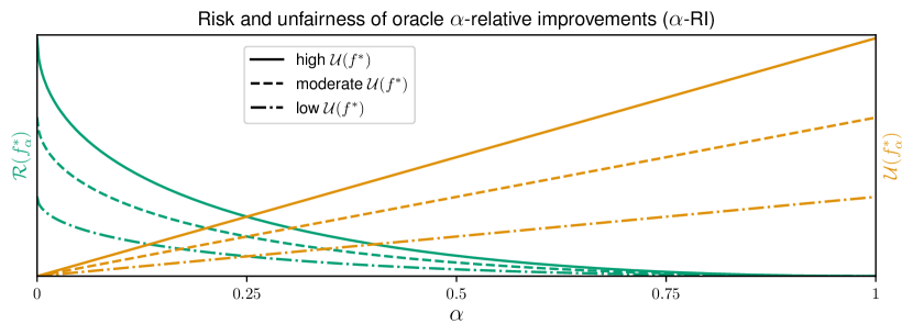
Figure 1: Risk \mathcal{R} and unfairness 𝒰𝒰\mathcal{U} of α𝛼\alpha-RI oracles {fα}α[0,1]subscriptsubscriptsuperscript𝑓𝛼𝛼01\{f^{*}_{\alpha}\}_{\alpha\in[0,1]}. Green curves (decreasing, convex) correspond to the risk, while orange curves (increasing, linear) correspond to the unfairness. Each pair of curves (solid, dashed, dashed dotted) corresponds to three regimes: high, moderate, and low unfairness of the regression function fsuperscript𝑓f^{*} respectively.

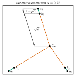
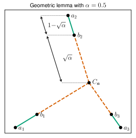
It has been shown that, under the squared loss, the optimal fair predictor f0subscriptsuperscript𝑓0f^{*}_{0} can be obtained as the solution of a Wasserstein-2 barycenter problem (Le Gouic, Loubes and Rigollet, 2020, Chzhen et al., 2020a). In Section 4 we study the whole family {fα}α[0,1]subscriptsubscriptsuperscript𝑓𝛼𝛼01\{f^{*}_{\alpha}\}_{\alpha\in[0,1]} for arbitrary choice of α[0,1]𝛼01\alpha\in[0,1]. To provide complete characterization of {fα}α[0,1]subscriptsubscriptsuperscript𝑓𝛼𝛼01\{f^{*}_{\alpha}\}_{\alpha\in[0,1]} we derive Lemma 4.3, which could be of independent interest. This result can be summarized as follows: given a fixed collection of points a1,,aKsubscript𝑎1subscript𝑎𝐾a_{1},\ldots,a_{K} in an abstract metric space (𝒳,d)𝒳𝑑(\mathcal{X},d), if one walks along the (constant speed) geodesics starting from assubscript𝑎𝑠a_{s} and leading to their (weighted) barycenter until it reaches a proportion α𝛼\alpha of the full path, then these intermediate points b1,,bKsubscript𝑏1subscript𝑏𝐾b_{1},\ldots,b_{K} minimize the weighted distance to the initial points while being α𝛼\alpha-closer to their own barycenter. This abstract result enables us to characterize explicitly oracle α𝛼\alpha-RI {fα}α[0,1]subscriptsubscriptsuperscript𝑓𝛼𝛼01\{f^{*}_{\alpha}\}_{\alpha\in[0,1]}. In particular, we show that the family of oracle α𝛼\alpha-RI {fα}α[0,1]subscriptsubscriptsuperscript𝑓𝛼𝛼01\{f^{*}_{\alpha}\}_{\alpha\in[0,1]} admits a simple structure: for any α[0,1]𝛼01\alpha\in[0,1] the prediction fαsubscriptsuperscript𝑓𝛼f^{*}_{\alpha} is the point-wise convex combination of the regression function ff1superscript𝑓subscriptsuperscript𝑓1f^{*}\equiv f^{*}_{1} and the optimal fair predictor f0subscriptsuperscript𝑓0f^{*}_{0}, that is,

fα(𝒙,s)=αf1(𝒙,s)+(1α)f0(𝒙,s),(𝒙,s)p×[K].formulae-sequencesubscriptsuperscript𝑓𝛼𝒙𝑠𝛼subscriptsuperscript𝑓1𝒙𝑠1𝛼superscriptsubscript𝑓0𝒙𝑠for-all𝒙𝑠superscript𝑝delimited-[]𝐾\displaystyle f^{*}_{\alpha}(\boldsymbol{x},s)=\sqrt{\alpha}f^{*}_{1}(\boldsymbol{x},s)+(1{-}\sqrt{\alpha})f_{0}^{*}(\boldsymbol{x},s),\qquad\forall\,(\boldsymbol{x},s)\in\mathbb{R}^{p}\times[K]\enspace.

The final contribution of Section 4 is the quantification of the risk-fairness trade-off on the population level. In particular, Lemma 4.5 establishes that for every α[0,1]𝛼01\alpha\in[0,1] it holds that

(fα)=(1α)2(f0)and𝒰(fα)=α𝒰(f).formulae-sequencesubscriptsuperscript𝑓𝛼superscript1𝛼2subscriptsuperscript𝑓0and𝒰subscriptsuperscript𝑓𝛼𝛼𝒰superscript𝑓\displaystyle\mathcal{R}(f^{*}_{\alpha})=(1{-}\sqrt{\alpha})^{2}\mathcal{R}(f^{*}_{0})\quad\text{and}\quad\mathcal{U}(f^{*}_{\alpha})=\alpha\,\mathcal{U}(f^{*})\enspace.

Observe that f0subscriptsuperscript𝑓0f^{*}_{0}, which is the optimal fair predictor in terms of DP, has the highest risk and the lowest unfairness, while the situation is reversed for f1fsubscriptsuperscript𝑓1superscript𝑓f^{*}_{1}\equiv f^{*} – the risk is the lowest and the unfairness is the highest. Since the function α(1α)2𝛼superscript1𝛼2\alpha\to(1{-}\sqrt{\alpha})^{2} grows rapidly in the vicinity of zero, even a mild relaxation of the exact fairness constraint (α=0)𝛼0(\alpha=0) yields a noticeable improvement in terms of the risk while having a low unfairness inflation. For instance, the risk of f1/2subscriptsuperscript𝑓12f^{*}_{\nicefrac{{1}}{{2}}} is only around 8.5%percent8.58.5\% of the risk of f0subscriptsuperscript𝑓0f^{*}_{0}, while its fairness is two times better than that of fsuperscript𝑓f^{*}. This observation is illustrated in Figure 1.

Minimax framework. In order to quantify the statistical price of fairness, in Section 5 we propose a minimax framework and in Section 5.1 we derive a general problem-dependent lower bound on the minimax risk of estimators satisfying the α𝛼\alpha-RI constraint. Statistical study of the model in Eq. (1) typically requires additional assumptions to provide meaningful statistical guarantees. Classically, one chooses a set \mathcal{F} of possible candidates for the regression function fsuperscript𝑓f^{*} (e.g., linear functions) and, possibly, introduces additional conditions on nuisance parameters of the model via some set ΘΘ\Theta (e.g., variance of the noise). The goal of our lower bound is to understand fundamental limits of the problem of prediction under α𝛼\alpha-RI constraint in arbitrary statistical model for Eq. (1). To this end, we show in Theorem 5.3 that any estimator f^^𝑓\hat{f} satisfying the α𝛼\alpha-RI constraint with high probability must incur

(f^)δn(,Θ)(1α)2𝒰(f),^𝑓subscript𝛿𝑛Θsuperscript1𝛼2𝒰superscript𝑓\displaystyle\mathcal{R}(\hat{f})\geq\delta_{n}(\mathcal{F},\Theta)\vee(1{-}\sqrt{\alpha})^{2}\mathcal{U}({f^{*}})\enspace,

where δn(,Θ)subscript𝛿𝑛Θ\delta_{n}(\mathcal{F},\Theta) is the rate one would obtain without restricting the set of possible estimators.

Application to linear model. The goal of Section 6 is to demonstrate that the general problem-dependent lower bound does indeed yield minimax optimal rates. To this end, we apply our machinery to the problem of linear regression with systematic bias formalized by the following linear model

Yi=𝑿i,𝜷+bSi+ξi,i=1,,n,formulae-sequencesubscript𝑌𝑖subscript𝑿𝑖superscript𝜷superscriptsubscript𝑏subscript𝑆𝑖subscript𝜉𝑖𝑖1𝑛\displaystyle Y_{i}=\left\langle\boldsymbol{X}_{i},\boldsymbol{\beta}^{*}\right\rangle+b_{S_{i}}^{*}+\xi_{i},\quad i=1,\dots,n\enspace,

where the ξisubscript𝜉𝑖\xi_{i}’s are i.i.d. zero mean Gaussian with variance σ2superscript𝜎2\sigma^{2} and the p𝑝p-dimensional covariates {𝑿i}i=1nsuperscriptsubscriptsubscript𝑿𝑖𝑖1𝑛\{\boldsymbol{X}_{i}\}_{i=1}^{n} are i.i.d. Gaussian random vectors. We propose an estimator f^^𝑓\hat{f} which, with probability at least 1δ1𝛿1-\delta, satisfies 𝒰(f^)α𝒰(f)𝒰^𝑓𝛼𝒰superscript𝑓\mathcal{U}(\hat{f})\leq\alpha\,\mathcal{U}(f^{*}) and achieves the following minimax optimal rate

(f^){σ2(p+Kn+log(1/δ)n)}{(1α)2𝒰(f)}.asymptotically-equals^𝑓superscript𝜎2𝑝𝐾𝑛1𝛿𝑛superscript1𝛼2𝒰superscript𝑓\displaystyle\mathcal{R}(\hat{f})\asymp\left\{\sigma^{2}\left({\frac{p+K}{n}}+{\frac{\log(\nicefrac{{1}}{{\delta}})}{n}}\right)\right\}\bigvee\bigg{\{}(1{-}\sqrt{\alpha})^{2}\mathcal{U}(f^{*})\bigg{\}}\enspace.

Finally, we conduct a simulation study of the proposed estimator f^^𝑓\hat{f} and compare its performance with more straightforward approaches in terms of unfairness and risk.

Ad-hoc procedure and experiments on CRIME dataset. The estimator that will be developed in the context of linear model with systematic bias relies heavily on the linear model and Gaussian features assumption. Thus, in Section 7, we propose a general post-processing estimator, which enjoys fairness and risk guarantees. Unlike the case of linear model, the optimality of these guarantees remains open. In Section 8, we provide empirical study of estimators from Sections 6 and 7, validating our theoretical claims numerically.

3 Prior and related works

Until very recently, contributions on fair regression were almost exclusively focused on the practical incorporation of proxy fairness constraints in classical learning methods, such as random forest, ridge regression, kernel based methods to name a few (Calders et al., 2013, Komiyama and Shimao, 2017, Berk et al., 2017, Pérez-Suay et al., 2017, Raff, Sylvester and Mills, 2018, Fitzsimons et al., 2018). Several works empirically study the impact of (relaxed) fairness constraints on the risk (Bertsimas, Farias and Trichakis, 2012, Zliobaite, 2015, Haas, 2019, Wick, Panda and Tristan, 2019, Zafar et al., 2017). Yet, the problem of precisely quantifying the effect of such constraints on the risk has not been tackled.

More recently, statistical and learning guarantees for fair regression were derived (Agarwal, Dudik and Wu, 2019, Le Gouic, Loubes and Rigollet, 2020, Chzhen et al., 2020a, Chiappa et al., 2020, Fitzsimons et al., 2019, Plečko and Meinshausen, 2020, Chzhen et al., 2020b). The closest works to our contribution are that of Le Gouic, Loubes and Rigollet (2020), Chzhen et al. (2020a), Chiappa et al. (2020), who draw a connection between the problem of exactly fair regression of demographic parity and the multi-marginal optimal transport formulation (Gangbo and Święch, 1998, Agueh and Carlier, 2011).

As already mentioned in the previous section, considering predictors which satisfy the DP constraint incurs an unavoidable price in terms of the risk. Depending on the application at hand, this price might or might not be reasonable. However, since the notion of DP is completely fairness driven, it does not allow to quantify the price of considering “fairer” predictions than the regression function fsuperscript𝑓f^{*}. For this reason, several contributions relax this constraint, forcing a milder fairness requirement. A natural idea is to define a functional 𝒰𝒰\mathcal{U} which quantifies the violation of the DP constraint and to declare a prediction approximately fair if this functional does not exceed a user pre-specified threshold. In recent years a large variety of such relaxations has been proposed: correlation based (Baharlouei et al., 2019, Mary, Calauzènes and El Karoui, 2019, Komiyama et al., 2018); Kolmogorov-Smirnov distance (Agarwal, Dudik and Wu, 2019); Mutual information (Steinberg et al., 2020, Steinberg, Reid and O’Callaghan, 2020); Total Variation distance (Oneto, Donini and Pontil, 2020, Oneto et al., 2020); Equality of means and higher moment matching (Raff, Sylvester and Mills, 2018, Fitzsimons et al., 2019, Calders et al., 2013, Berk et al., 2017, Olfat et al., 2020, Donini et al., 2018); Maximum Mean Discrepancy (Quadrianto and Sharmanska, 2017, Madras et al., 2018); Wasserstein distance (Chiappa et al., 2020, Le Gouic, Loubes and Rigollet, 2020, Chzhen et al., 2020a, Gordaliza et al., 2019).

3.1 Other notions of unfairness

The most common relaxations of the Demographic Parity constraint are based on the Total Variation (TV) and the Kolmogorov-Smirnov (KS) distances (Agarwal, Dudik and Wu, 2019, Oneto, Donini and Pontil, 2020, Agarwal et al., 2018, Chzhen et al., 2020b). There are various ways to use the TV or KS in order to build a functional 𝒰𝒰\mathcal{U}, which quantifies the violation of the DP constraint. To compare those measures of discrepancy with the one that we introduce in our work, we define 𝒰TVsubscript𝒰TV\mathcal{U}_{\operatorname{TV}} and 𝒰KSsubscript𝒰KS\mathcal{U}_{\operatorname{KS}} as follows

TV unfairness: 𝒰TV(f):=s[K]TV(Law(f(𝑿,S)S=s),Law(f(𝑿,S))),assignsubscript𝒰TV𝑓subscript𝑠delimited-[]𝐾TVLawconditional𝑓𝑿𝑆𝑆𝑠Law𝑓𝑿𝑆\displaystyle\mathcal{U}_{\operatorname{TV}}(f)\vcentcolon=\sum_{s\in[K]}\operatorname{TV}\left(\operatorname{Law}(f(\boldsymbol{X},S)\mid S=s),\,\operatorname{Law}(f(\boldsymbol{X},S))\right)\enspace,
KS unfairness: 𝒰KS(f):=s[K]KS(Law(f(𝑿,S)S=s),Law(f(𝑿,S))).assignsubscript𝒰KS𝑓subscript𝑠delimited-[]𝐾KSLawconditional𝑓𝑿𝑆𝑆𝑠Law𝑓𝑿𝑆\displaystyle\mathcal{U}_{\operatorname{KS}}(f)\vcentcolon=\sum_{s\in[K]}\operatorname{KS}\left(\operatorname{Law}(f(\boldsymbol{X},S)\mid S=s),\,\operatorname{Law}(f(\boldsymbol{X},S))\right)\enspace.

Using these notions, one wishes to study those predictors f𝑓f which satisfy relaxed fairness constraint 𝒰(f)εsubscript𝒰𝑓𝜀\mathcal{U}_{\square}(f)\leq\varepsilon, where \square is KSKS\operatorname{KS} or TVTV\operatorname{TV} and ε0𝜀0\varepsilon\geq 0 is a user specified parameter. Note that since both KSKS\operatorname{KS} and TVTV\operatorname{TV} are metrics, setting ε=0𝜀0\varepsilon=0 is equivalent to the DP constraint. Meanwhile, for ε>0𝜀0\varepsilon>0 these formulations allow some slack. It is known that the TV distance is rather strong and extremely sensitive to small changes in distributions which is the major drawback of the TV unfairness. This limitation can be addressed by the KS unfairness due to an obvious relation 𝒰KS(f)𝒰TV(f)subscript𝒰KS𝑓subscript𝒰TV𝑓\mathcal{U}_{\operatorname{KS}}(f)\leq\mathcal{U}_{\operatorname{TV}}(f).

In our work we argue that the introduced notion of unfairness 𝒰𝒰\mathcal{U} is better suited for the problem of regression with squared loss under fairness constraint. Indeed, we prove in Lemma 4.5 that 𝒰𝒰\mathcal{U} can be naturally connected to the squared risk and allows to give a precise quantification of the risk-fairness trade-off. This result is the major advantage of 𝒰𝒰\mathcal{U} over both 𝒰KSsubscript𝒰KS\mathcal{U}_{\operatorname{KS}} and 𝒰TVsubscript𝒰TV\mathcal{U}_{\operatorname{TV}}. Nevertheless, it is still interesting to understand whether a more popular KSKS\operatorname{KS} unfairness can be related to 𝒰𝒰\mathcal{U} that we introduce. In Appendix we prove the following connection.

Proposition 3.1.

Fix some predictor f:p×[K]:𝑓superscript𝑝delimited-[]𝐾f:\mathbb{R}^{p}\times[K]\to\mathbb{R}. Assume that Law(f(𝐗,S)S=s)𝒫2()Lawconditional𝑓𝐗𝑆𝑆𝑠subscript𝒫2\operatorname{Law}(f(\boldsymbol{X},S)\mid S{=}s)\in\mathcal{P}_{2}(\mathbb{R}) and it admits density bounded by Cf,s>0subscript𝐶𝑓𝑠0C_{f,s}>0 for all s[K]𝑠delimited-[]𝐾s\in[K], then333One can erase 1/𝐰subscriptnorm1𝐰\|\nicefrac{{1}}{{\boldsymbol{w}}}\|_{\infty} from the bound introducing these weights into the definition of 𝒰KS(f)subscript𝒰KS𝑓\mathcal{U}_{\operatorname{KS}}(f).

𝒰KS(f)1/𝒘8C¯f𝒰1/4(f),subscript𝒰KS𝑓subscriptnorm1𝒘8subscript¯𝐶𝑓superscript𝒰14𝑓\displaystyle\mathcal{U}_{\operatorname{KS}}(f)\leq\|\nicefrac{{1}}{{\boldsymbol{w}}}\|_{\infty}\sqrt{8\bar{C}_{f}}\cdot\mathcal{U}^{1/4}(f)\enspace,

where C¯f=s=1KwsCf,ssubscript¯𝐶𝑓superscriptsubscript𝑠1𝐾subscript𝑤𝑠subscript𝐶𝑓𝑠\bar{C}_{f}=\sum_{s=1}^{K}w_{s}C_{f,s} and 1/𝐰=(1/w1,,1/wK)1𝐰superscript1subscript𝑤11subscript𝑤𝐾top\nicefrac{{1}}{{\boldsymbol{w}}}=(\nicefrac{{1}}{{w_{1}}},\ldots,\nicefrac{{1}}{{w_{K}}})^{\top}.

The latter result indicates that if one can control the unfairness 𝒰𝒰\mathcal{U} introduced in this work, one also has some control over the KSKS\operatorname{KS} unfairness. Note that the leading constant of the previous bound depends on the predictor f𝑓f. More precisely, this constant corresponds to the upper bound on the density of f(𝑿,S)𝑓𝑿𝑆f(\boldsymbol{X},S).

Another advantage of the introduced unfairness measure, and, in particular, the notion of α𝛼\alpha-relative improvement is the fact that the parameter α𝛼\alpha has a clear practical interpretation, while the interpretation of ε𝜀\varepsilon is not intuitive. Of course, using 𝒰KSsubscript𝒰KS\mathcal{U}_{\operatorname{KS}} or 𝒰TVsubscript𝒰TV\mathcal{U}_{\operatorname{TV}} one can also define unfairness of a predictor f𝑓f relatively to the regression function fsuperscript𝑓f^{*}. However, the interpretation of KSKS\operatorname{KS} or TVTV\operatorname{TV} unfairness relative to the unfairness of the Bayes rule is less meaningful. Indeed, intuitively, if a prediction function f:p×[K]:𝑓superscript𝑝delimited-[]𝐾f:\mathbb{R}^{p}\times[K]\to\mathbb{R} introduces some group-wise disparities, then cf𝑐𝑓c\cdot f for c1much-greater-than𝑐1c\gg 1 should be even further amplifying these disparities. Yet, for all c>0𝑐0c>0 we have 𝒰KS/TV(cf)=𝒰KS/TV(f)subscript𝒰KSTV𝑐𝑓subscript𝒰KSTV𝑓\mathcal{U}_{\operatorname{KS}/\operatorname{TV}}(c\cdot f)=\mathcal{U}_{\operatorname{KS}/\operatorname{TV}}(f), while the introduced notion of unfairness satisfies 𝒰(cf)=c2𝒰(f)𝒰𝑐𝑓superscript𝑐2𝒰𝑓\mathcal{U}(c\cdot f)=c^{2}\mathcal{U}(f) for all c>0𝑐0c>0. Due to completely different geometries induced by \mathcal{R} in the space of functions and by 𝒰KS/TVsubscript𝒰KSTV\mathcal{U}_{\operatorname{KS}{/}\operatorname{TV}} in the space of distributions, precise theoretical study of such formulations is notoriously complicated if possible.

3.2 Optimal transport and fair regression

The use of optimal transport tools in the study of fairness is relatively recent. Initially, contributions in this direction were mainly dealing with the problem of binary classification (Gordaliza et al., 2019, Jiang et al., 2020). Later on, the tools of the optimal transport theory migrated to the setup of fair regression (Chiappa et al., 2020, Chzhen et al., 2020a, Le Gouic, Loubes and Rigollet, 2020). The main theoretical motivation to consider 𝒰𝒰\mathcal{U} instead of the KS and TV unfairnesses lies in the following recent result.

Theorem 3.2 (Le Gouic, Loubes and Rigollet (2020), Chzhen et al. (2020a)).

Let Assumption 2.1 be satisfied, then

min{(f):(f(𝑿,S)S=s)=d(f(𝑿,S)S=s)s,s[K]}=𝒰(f).:𝑓formulae-sequencesuperscript𝑑conditional𝑓𝑿𝑆𝑆𝑠conditional𝑓𝑿𝑆𝑆superscript𝑠for-all𝑠superscript𝑠delimited-[]𝐾𝒰superscript𝑓\displaystyle\min\left\{\mathcal{R}(f)\,:\,\big{(}f(\boldsymbol{X},S)\mid S=s\big{)}\leavevmode\mathrel{\mathop{=}\limits^{d}}\big{(}f(\boldsymbol{X},S)\mid S=s^{\prime}\big{)}\,\,\forall s,s^{\prime}\in[K]\right\}=\mathcal{U}(f^{*})\enspace. (2)

Moreover, the distribution of the minimizer of the problem on the l.h.s. is given by

argminν𝒫2()s=1Kws𝖶22(Law(f(𝑿,S)S=s),ν).subscriptargmin𝜈subscript𝒫2superscriptsubscript𝑠1𝐾subscript𝑤𝑠superscriptsubscript𝖶22Lawconditionalsuperscript𝑓𝑿𝑆𝑆𝑠𝜈\displaystyle\operatorname*{arg\,min}_{\nu\in\mathcal{P}_{2}(\mathbb{R})}\sum_{s=1}^{K}w_{s}\mathsf{W}_{2}^{2}\left(\operatorname{Law}(f^{*}(\boldsymbol{X},S)\mid S{=}s),\,\nu\right)\enspace.

An important consequence of Theorem 3.2 is that it puts the risk \mathcal{R} and the unfairness 𝒰𝒰\mathcal{U} – two conflicting quantities – on the same scale. In particular, it allows to measure both fairness and risk using the same unit measurements, hence, study the trade-off between the two. In order to build our framework, we remark that since 𝖶2subscript𝖶2\mathsf{W}_{2} is a metric then the problem on the l.h.s. of Eq. (2) can be equivalently written as min{(f):𝒰(f)0×𝒰(f)}:𝑓𝒰𝑓0𝒰superscript𝑓\min\left\{\mathcal{R}(f)\,:\,\mathcal{U}(f)\leq 0\times\mathcal{U}(f^{*})\right\}. Moreover, one can observe that the regression function fmin{(f):𝒰(f)1×𝒰(f)}superscript𝑓:𝑓𝒰𝑓1𝒰superscript𝑓f^{*}\in\min\left\{\mathcal{R}(f)\,:\,\mathcal{U}(f)\leq 1\times\mathcal{U}(f^{*})\right\}. Thus, a natural relaxation of the above formulation is the introduced notion of α𝛼\alpha-relative improvement, which interpolates between the exactly fair predictor f0subscriptsuperscript𝑓0f^{*}_{0} and the regression function f1fsubscriptsuperscript𝑓1superscript𝑓f^{*}_{1}\equiv f^{*}. In this retrospect, the result of Le Gouic, Loubes and Rigollet (2020), Chzhen et al. (2020a) provides characterization of f0subscriptsuperscript𝑓0f^{*}_{0} but says nothing about the whole family of oracle α𝛼\alpha-RI {fα}α[0,1]subscriptsubscriptsuperscript𝑓𝛼𝛼01\{f^{*}_{\alpha}\}_{\alpha\in[0,1]}.

4 Oracle α𝛼\alpha-relative improvement

This section is devoted to the study of the α𝛼\alpha-relative improvement fαsubscriptsuperscript𝑓𝛼f^{*}_{\alpha} on population level, that is, in this section we study

fαargmin{(f):𝒰(f)α𝒰(f)},α[0,1].formulae-sequencesubscriptsuperscript𝑓𝛼argmin:𝑓𝒰𝑓𝛼𝒰superscript𝑓for-all𝛼01\displaystyle f^{*}_{\alpha}\in\operatorname*{arg\,min}\left\{\mathcal{R}(f)\,:\,\mathcal{U}(f)\leq\alpha\,\mathcal{U}(f^{*})\right\}\enspace,\qquad\forall\alpha\in[0,1]\enspace. (3)

The next result establishes a closed form solution to the minimization Problem (3) under Assumption 2.1 for any value of α[0,1]𝛼01\alpha\in[0,1].

Proposition 4.1.

Let Assumption 2.1 be satisfied, then for all α[0,1]𝛼01\alpha\in[0,1] and all (𝐱,s)p×[K]𝐱𝑠superscript𝑝delimited-[]𝐾(\boldsymbol{x},s)\in\mathbb{R}^{p}\times[K] (up to a set of null measure) it holds that

fα(𝒙,s)superscriptsubscript𝑓𝛼𝒙𝑠\displaystyle f_{\alpha}^{*}(\boldsymbol{x},s) =αf(𝒙,s)+(1α)s=1KwsFνs1Fνsf(𝒙,s)absent𝛼superscript𝑓𝒙𝑠1𝛼superscriptsubscriptsuperscript𝑠1𝐾subscript𝑤superscript𝑠superscriptsubscript𝐹subscriptsuperscript𝜈superscript𝑠1subscript𝐹subscriptsuperscript𝜈𝑠superscript𝑓𝒙𝑠\displaystyle=\sqrt{\alpha}f^{*}(\boldsymbol{x},s)+\big{(}1{-}\sqrt{\alpha}\big{)}\sum_{s^{\prime}=1}^{K}w_{s^{\prime}}F_{\nu^{*}_{s^{\prime}}}^{-1}\circ F_{\nu^{*}_{s}}\circ f^{*}(\boldsymbol{x},s)
=αf1(𝒙,s)+(1α)f0(𝒙,s).absent𝛼subscriptsuperscript𝑓1𝒙𝑠1𝛼superscriptsubscript𝑓0𝒙𝑠\displaystyle=\sqrt{\alpha}f^{*}_{1}(\boldsymbol{x},s)+(1{-}\sqrt{\alpha})f_{0}^{*}(\boldsymbol{x},s)\enspace.

Recall that f=f1superscript𝑓subscriptsuperscript𝑓1f^{*}=f^{*}_{1}, hence the α𝛼\alpha-relative improvement fαsubscriptsuperscript𝑓𝛼f^{*}_{\alpha} is the point-wise convex combination of exactly fair prediction f0subscriptsuperscript𝑓0f^{*}_{0} and the regression function f1subscriptsuperscript𝑓1f^{*}_{1}. Besides, setting α=0𝛼0\alpha=0 we recover the result of Chzhen et al. (2020a), Le Gouic, Loubes and Rigollet (2020) as a particular case of our framework.

[Uncaptioned image]
[Uncaptioned image][Uncaptioned image]
Figure 2: Impact of the weights 𝒘ΔK1𝒘superscriptΔ𝐾1\boldsymbol{w}\in\Delta^{K-1} on the distribution of f0subscriptsuperscript𝑓0f^{*}_{0}

Let Assumption 2.1 be satisfied, then the set of oracle α𝛼\alpha-RI {fα}α[0,1]subscriptsubscriptsuperscript𝑓𝛼𝛼01\{f^{*}_{\alpha}\}_{\alpha\in[0,1]} satisfies the following properties.

  1. 1.

    Risk and fairness monotonicity: if αα𝛼superscript𝛼\alpha\leq\alpha^{\prime}, then (fα)(fα)superscriptsubscript𝑓𝛼subscriptsuperscript𝑓superscript𝛼\mathcal{R}(f_{\alpha}^{*})\geq\mathcal{R}(f^{*}_{\alpha^{\prime}}) and 𝒰(fα)𝒰(fα)𝒰subscriptsuperscript𝑓𝛼𝒰subscriptsuperscript𝑓superscript𝛼\mathcal{U}(f^{*}_{\alpha})\leq\mathcal{U}(f^{*}_{\alpha^{\prime}}).

  2. 2.

    Point-wise convexity: for all α,α[0,1]𝛼superscript𝛼01\alpha,\alpha^{\prime}\in[0,1] and all τ[0,1]𝜏01\tau\in[0,1] it holds that τfα+(1τ)fα{fα}α[0,1]𝜏subscriptsuperscript𝑓𝛼1𝜏subscriptsuperscript𝑓superscript𝛼subscriptsubscriptsuperscript𝑓𝛼𝛼01\tau f^{*}_{\alpha}+(1-\tau)f^{*}_{\alpha^{\prime}}\in\{f^{*}_{\alpha}\}_{\alpha\in[0,1]}. Moreover τfα+(1τ)fα=fα¯𝜏subscriptsuperscript𝑓𝛼1𝜏subscriptsuperscript𝑓superscript𝛼subscriptsuperscript𝑓¯𝛼\tau f^{*}_{\alpha}+(1-\tau)f^{*}_{\alpha^{\prime}}=f^{*}_{\bar{\alpha}} with α¯=(τα+(1τ)α)2¯𝛼superscript𝜏𝛼1𝜏superscript𝛼2\bar{\alpha}=(\tau\sqrt{\alpha}+(1-\tau)\sqrt{\alpha^{\prime}})^{2}.

  3. 3.

    Order preservation: for all s[K],𝒙,𝒙pformulae-sequence𝑠delimited-[]𝐾𝒙superscript𝒙superscript𝑝s\in[K],\boldsymbol{x},\boldsymbol{x}^{\prime}\in\mathbb{R}^{p}, if f(𝒙,s)f(𝒙,s)superscript𝑓𝒙𝑠superscript𝑓superscript𝒙𝑠f^{*}(\boldsymbol{x},s)\geq f^{*}(\boldsymbol{x}^{\prime},s), then for all α[0,1]𝛼01\alpha\in[0,1] it holds that fα(𝒙,s)fα(𝒙,s)subscriptsuperscript𝑓𝛼𝒙𝑠subscriptsuperscript𝑓𝛼superscript𝒙𝑠f^{*}_{\alpha}(\boldsymbol{x},s)\geq f^{*}_{\alpha}(\boldsymbol{x}^{\prime},s).

  4. 4.

    Average stability: let μssubscriptsuperscript𝜇𝑠\mu^{*}_{s} be the expected value of νssubscriptsuperscript𝜈𝑠\nu^{*}_{s}. For all α[0,1]𝛼01\alpha\in[0,1] and all 𝒘=(w1,,wK)ΔK1superscript𝒘superscriptsuperscriptsubscript𝑤1superscriptsubscript𝑤𝐾topsuperscriptΔ𝐾1\boldsymbol{w}^{\prime}=(w_{1}^{\prime},\ldots,w_{K}^{\prime})^{\top}\in\Delta^{K-1} it holds that

    s=1Kws𝔼[fα(𝑿,S)S=s]=α(s=1Kwsμs)+(1α)(s=1Kwsμs).superscriptsubscript𝑠1𝐾superscriptsubscript𝑤𝑠𝔼delimited-[]conditionalsubscriptsuperscript𝑓𝛼𝑿𝑆𝑆𝑠𝛼superscriptsubscript𝑠1𝐾superscriptsubscript𝑤𝑠subscriptsuperscript𝜇𝑠1𝛼superscriptsubscript𝑠1𝐾subscript𝑤𝑠superscriptsubscript𝜇𝑠\displaystyle\sum_{s=1}^{K}w_{s}^{\prime}\mathbb{E}[f^{*}_{\alpha}(\boldsymbol{X},S)\mid S=s]=\sqrt{\alpha}\left(\sum_{s=1}^{K}w_{s}^{\prime}\mu^{*}_{s}\right)+(1{-}\sqrt{\alpha})\left(\sum_{s=1}^{K}w_{s}\mu_{s}^{*}\right)\enspace.

    In particular, setting 𝒘=𝒘superscript𝒘𝒘\boldsymbol{w}^{\prime}=\boldsymbol{w}, we get for all α[0,1]𝛼01\alpha\in[0,1] the average stability:

    s=1Kws𝔼[fα(𝑿,S)S=s]=s=1Kws𝔼[f(𝑿,S)S=s].superscriptsubscript𝑠1𝐾subscript𝑤𝑠𝔼delimited-[]conditionalsubscriptsuperscript𝑓𝛼𝑿𝑆𝑆𝑠superscriptsubscript𝑠1𝐾subscript𝑤𝑠𝔼delimited-[]conditionalsuperscript𝑓𝑿𝑆𝑆𝑠\displaystyle\sum_{s=1}^{K}w_{s}\mathbb{E}[f^{*}_{\alpha}(\boldsymbol{X},S)\mid S=s]=\sum_{s=1}^{K}w_{s}\mathbb{E}[f^{*}(\boldsymbol{X},S)\mid S=s]\enspace.

The first property is intuitive and does not require the result of Proposition 4.1. The second property can be directly derived using the expression of fαsubscriptsuperscript𝑓𝛼f^{*}_{\alpha} and it describes additional algebraic structure of the family {fα}α[0,1]subscriptsubscriptsuperscript𝑓𝛼𝛼01\{f^{*}_{\alpha}\}_{\alpha\in[0,1]} . The third group-wise order preserving property of fαsubscriptsuperscript𝑓𝛼f^{*}_{\alpha} is particularly attractive. Its proof is straightforward after the observation that Fνssubscript𝐹superscriptsubscript𝜈𝑠F_{\nu_{s}^{*}} and s=1KwsFνs1superscriptsubscriptsuperscript𝑠1𝐾subscript𝑤superscript𝑠subscriptsuperscript𝐹1subscriptsuperscript𝜈superscript𝑠\sum_{s^{\prime}=1}^{K}w_{s^{\prime}}F^{-1}_{\nu^{*}_{s^{\prime}}} are non-decreasing functions and the fact that the composition of two non-decreasing functions is non-decreasing. For the special case of α=0𝛼0\alpha=0, this observation has already been made in (Chzhen et al., 2020a) and a practical algorithm that follows the group-wise order preservation property was proposed by Plečko and Meinshausen (2020). In the context of classification Lipton, Chouldechova and McAuley (2018) refer to this property as “rational ordering”. In words, this property says: given any two individuals 𝒙,𝒙p𝒙superscript𝒙superscript𝑝\boldsymbol{x},\boldsymbol{x}^{\prime}\in\mathbb{R}^{p} from the same sensitive group s[K]𝑠delimited-[]𝐾s\in[K], if the optimal prediction f(𝒙,s)superscript𝑓𝒙𝑠f^{*}(\boldsymbol{x},s) for 𝒙𝒙\boldsymbol{x} is larger than that for 𝒙superscript𝒙\boldsymbol{x}^{\prime}, then across all levels α𝛼\alpha of fairness parameter the oracle α𝛼\alpha-RI fαsubscriptsuperscript𝑓𝛼f^{*}_{\alpha} is not changing this order. The last property of average stability admits an interesting interpretation. Let us interpret f:p×𝒮+:𝑓superscript𝑝𝒮subscriptf:\mathbb{R}^{p}\times\mathcal{S}\to\mathbb{R}_{+} as a salary assignment function (making it naturally positive). In that case setting 𝒘=𝒘=(1/K,,1/K)superscript𝒘𝒘superscript1𝐾1𝐾top\boldsymbol{w}^{\prime}=\boldsymbol{w}=(\nicefrac{{1}}{{K}},\ldots,\nicefrac{{1}}{{K}})^{\top}, we can interpret 𝔼[f(𝑿,S)S=s]𝔼delimited-[]conditionalsuperscript𝑓𝑿𝑆𝑆𝑠\mathbb{E}[f^{*}(\boldsymbol{X},S)\mid S=s] as the average amount of money allocated for salaries within group s𝒮𝑠𝒮s\in\mathcal{S}. Thus, in this context, the average stability property states that by enforcing fairness improvement property with equally distributed weights across groups 𝒘=(1/K,,1/K)𝒘superscript1𝐾1𝐾top\boldsymbol{w}=(\nicefrac{{1}}{{K}},\ldots,\nicefrac{{1}}{{K}})^{\top}, we do not need to augment the budget allocated for these salaries. The proof of the last property is also rather straightforward: for every s𝒮𝑠𝒮s\in\mathcal{S} define the mean of the distribution νssubscriptsuperscript𝜈𝑠\nu^{*}_{s} as ms:=𝔼[f(𝑿,S)S=s]assignsuperscriptsubscript𝑚𝑠𝔼delimited-[]conditionalsuperscript𝑓𝑿𝑆𝑆𝑠m_{s}^{*}\vcentcolon=\mathbb{E}[f^{*}(\boldsymbol{X},S)\mid S=s], then

𝔼[fα(𝑿,S)S=s]𝔼delimited-[]conditionalsuperscriptsubscript𝑓𝛼𝑿𝑆𝑆𝑠\displaystyle\mathbb{E}[f_{\alpha}^{*}(\boldsymbol{X},S)\mid S=s] =αms+(1α)s=1Kws𝔼[Fνs1Fνsf(𝑿,S)S=s].absent𝛼subscriptsuperscript𝑚𝑠1𝛼superscriptsubscriptsuperscript𝑠1𝐾subscript𝑤superscript𝑠𝔼delimited-[]conditionalsuperscriptsubscript𝐹subscriptsuperscript𝜈superscript𝑠1subscript𝐹subscriptsuperscript𝜈𝑠superscript𝑓𝑿𝑆𝑆𝑠\displaystyle=\sqrt{\alpha}m^{*}_{s}+\big{(}1{-}\sqrt{\alpha}\big{)}\sum_{s^{\prime}=1}^{K}w_{s^{\prime}}\mathbb{E}\left[F_{\nu^{*}_{s^{\prime}}}^{-1}\circ F_{\nu^{*}_{s}}\circ f^{*}(\boldsymbol{X},S)\mid S=s\right]\enspace.

To conclude, it suffices to notice that under Assumption 2.1 the random variable (Fνs1Fνsf(𝑿,S)S=s)conditionalsuperscriptsubscript𝐹subscriptsuperscript𝜈superscript𝑠1subscript𝐹subscriptsuperscript𝜈𝑠superscript𝑓𝑿𝑆𝑆𝑠(F_{\nu^{*}_{s^{\prime}}}^{-1}\circ F_{\nu^{*}_{s}}\circ f^{*}(\boldsymbol{X},S)\mid S=s) is distributed according to νssubscriptsuperscript𝜈superscript𝑠\nu^{*}_{s^{\prime}}.

4.1 Influence of the choice of weights

Note that the considered framework permits the statistician to pick different 𝒘ΔK1𝒘superscriptΔ𝐾1\boldsymbol{w}\in\Delta^{K-1}. To study this additional level of flexibility and freedom, we provide in this section the intuition for three natural choices:

  • Proportional: ws=(S=s)subscript𝑤𝑠𝑆𝑠w_{s}=\mathbb{P}(S=s);

  • Inverse: ws1/(S=s)similar-tosubscript𝑤𝑠1𝑆𝑠w_{s}\sim 1/\mathbb{P}(S=s);

  • Equal weights: ws=1Ksubscript𝑤𝑠1𝐾w_{s}=\tfrac{1}{K}.

Since all of the α𝛼\alpha-RI prediction functions can be obtained as convex combination of f0subscriptsuperscript𝑓0f^{*}_{0} and the Bayes rule, it is sufficient to understand the underlying principle behind f0subscriptsuperscript𝑓0f^{*}_{0}. We focus on the case of two groups (K=2𝐾2K=2), with the first group representing the minority ((S=1)(S=2))much-less-than𝑆1𝑆2(\mathbb{P}(S=1)\ll\mathbb{P}(S=2)). As already mentioned, the Bayes optimal prediction fsuperscript𝑓f^{*} induces two distributions ν1subscriptsuperscript𝜈1\nu^{*}_{1} and ν2subscriptsuperscript𝜈2\nu^{*}_{2} (e.g., distribution of salaries for minority and majority sub-populations). We schematically illustrate these distributions on top left plot of Fig. 4.

The choice of ws=(S=s)subscript𝑤𝑠𝑆𝑠w_{s}=\mathbb{P}(S=s) (bottom left on Fig. 4) leads to equalization of minority to majority—that is, the situation of the majority group is modified only slightly, while the minority gets pushed towards the majority; the choice ws1/(S=s)similar-tosubscript𝑤𝑠1𝑆𝑠w_{s}\sim 1/\mathbb{P}(S=s) (bottom right on Fig. 4) leads to an inverse situation—majority is equalized to minority; the choice ws=1/Ksubscript𝑤𝑠1𝐾w_{s}=1/K (top right on Fig. 4) leads to a “middle ground” compromise, where both the majority and the minority are pushed toward their barycenter. The actual choice of the weights clearly depends on the given application and the social aspects of thereof. We hope that the provided intuition in conjunction with domain expertise can help the practitioner to make a more informed choice for the weights.

4.2 An abstract geometric lemma

The proof of Proposition 4.1 relies on an abstract geometric result, Lemma 4.3, which might be interesting on its own. First, let us introduce the following definition, which asks for existence of finitely supported barycenters in a metric space (𝒳,d)𝒳𝑑(\mathcal{X},d).

Definition 4.2 (Barycenter property).

We say that a metric space (𝒳,d)𝒳𝑑(\mathcal{X},d) satisfies the barycenter property if for any weights 𝐰ΔK1𝐰superscriptΔ𝐾1\boldsymbol{w}\in\Delta^{K-1} and tuple 𝐚=(a1,,aK)𝒳K𝐚subscript𝑎1subscript𝑎𝐾superscript𝒳𝐾\boldsymbol{a}=(a_{1},\ldots,a_{K})\in\mathcal{X}^{K} there exists a barycenter

C𝒂𝒘argminC𝒳s=1Kwsd2(as,C).subscript𝐶subscript𝒂𝒘subscriptargmin𝐶𝒳superscriptsubscript𝑠1𝐾subscript𝑤𝑠superscript𝑑2subscript𝑎𝑠𝐶\displaystyle C_{\boldsymbol{a}_{\boldsymbol{w}}}\in\operatorname*{arg\,min}_{C\in\mathcal{X}}\sum_{s=1}^{K}w_{s}d^{2}(a_{s},C)\enspace.

Moreover, for any tuple 𝐚=(a1,,aK)𝒳K𝐚subscript𝑎1subscript𝑎𝐾superscript𝒳𝐾\boldsymbol{a}=(a_{1},\ldots,a_{K})\in\mathcal{X}^{K} we denote444When there is no ambiguity in the weights 𝐰𝐰\boldsymbol{w} we simply write C𝐚subscript𝐶𝐚C_{\boldsymbol{a}}. by C𝐚𝐰subscript𝐶subscript𝐚𝐰C_{\boldsymbol{a}_{\boldsymbol{w}}} a barycenter of 𝐚𝐚\boldsymbol{a} weighted by 𝐰ΔK1𝐰superscriptΔ𝐾1\boldsymbol{w}\in\Delta^{K-1}.

Refer to caption
Refer to caption
Refer to caption
Figure 3: Illustration of Lemma 4.3 for (𝒳,d)=(2,2)(\mathcal{X},d)=(\mathbb{R}^{2},\|\cdot\|_{2}) and α{0.25,0.5,0.75}𝛼0.250.50.75\alpha\in\{0.25,0.5,0.75\}. The initial points a1,a2,a3subscript𝑎1subscript𝑎2subscript𝑎3a_{1},a_{2},a_{3} are the vertices of an isosceles triangle. The weights are set as follows: w1=0.1subscript𝑤10.1w_{1}=0.1, w2=0.4subscript𝑤20.4w_{2}=0.4 and w3=0.5subscript𝑤30.5w_{3}=0.5.
Lemma 4.3 (Abstract geometric lemma).

Let (𝒳,d)𝒳𝑑(\mathcal{X},d) be a metric space satisfying the q𝑞q-barycenter property. Let 𝐚=(a1,,aK)𝒳K𝐚subscript𝑎1subscript𝑎𝐾superscript𝒳𝐾\boldsymbol{a}=(a_{1},\ldots,a_{K})\in\mathcal{X}^{K}, 𝐰=(w1,,wK)ΔK1𝐰superscriptsubscript𝑤1subscript𝑤𝐾topsuperscriptΔ𝐾1\boldsymbol{w}=(w_{1},\ldots,w_{K})^{\top}\in\Delta^{K-1} and let C𝐚subscript𝐶𝐚C_{\boldsymbol{a}} be a barycenter of 𝐚𝐚\boldsymbol{a} with respect to weights 𝐰𝐰\boldsymbol{w}. For a fixed α[0,1]𝛼01\alpha\in[0,1] assume that there exists 𝐛=(b1,,bK)𝒳K𝐛subscript𝑏1subscript𝑏𝐾superscript𝒳𝐾\boldsymbol{b}=(b_{1},\ldots,b_{K})\in\mathcal{X}^{K} which satisfies

d(as,C𝒂)=d(as,bs)+d(bs,C𝒂),𝑑subscript𝑎𝑠subscript𝐶𝒂𝑑subscript𝑎𝑠subscript𝑏𝑠𝑑subscript𝑏𝑠subscript𝐶𝒂\displaystyle d(a_{s},C_{\boldsymbol{a}})=d(a_{s},b_{s})+d(b_{s},C_{\boldsymbol{a}})\enspace,\qquad s=1,,K,𝑠1𝐾\displaystyle s=1,\dots,K\enspace, (P1subscript𝑃1P_{1})
d(bs,as)=(1α1/2)d(as,C𝒂),𝑑subscript𝑏𝑠subscript𝑎𝑠1superscript𝛼12𝑑subscript𝑎𝑠subscript𝐶𝒂\displaystyle d(b_{s},a_{s})=\big{(}1{-}\alpha^{\nicefrac{{1}}{{2}}}\big{)}d(a_{s},C_{\boldsymbol{a}})\enspace,\qquad s=1,,K.𝑠1𝐾\displaystyle s=1,\dots,K\enspace. (P2subscript𝑃2P_{2})

Then, 𝐛𝐛\boldsymbol{b} is a solution of

inf𝒃𝒳K{s=1Kwsd2(bs,as):s=1Kwsd2(bs,C𝒃)αs=1Kwsd2(as,C𝒂)}.subscriptinfimum𝒃superscript𝒳𝐾conditional-setsuperscriptsubscript𝑠1𝐾subscript𝑤𝑠superscript𝑑2subscript𝑏𝑠subscript𝑎𝑠superscriptsubscript𝑠1𝐾subscript𝑤𝑠superscript𝑑2subscript𝑏𝑠subscript𝐶𝒃𝛼superscriptsubscript𝑠1𝐾subscript𝑤𝑠superscript𝑑2subscript𝑎𝑠subscript𝐶𝒂\displaystyle\inf_{\boldsymbol{b}\in\mathcal{X}^{K}}\left\{\sum_{s=1}^{K}w_{s}d^{2}(b_{s},a_{s})\,:\,\sum_{s=1}^{K}w_{s}d^{2}(b_{s},C_{\boldsymbol{b}})\leq{\alpha}\sum_{s=1}^{K}w_{s}d^{2}(a_{s},C_{\boldsymbol{a}})\right\}\enspace. (4)
Remark 4.4.

Property (P1subscript𝑃1P_{1}) essentially requires that each bisubscript𝑏𝑖b_{i} lies on the geodesic between aisubscript𝑎𝑖a_{i} and C𝐚subscript𝐶𝐚C_{\boldsymbol{a}} while Property (P2subscript𝑃2P_{2}) specifies the location of bisubscript𝑏𝑖b_{i} on this geodesic: bisubscript𝑏𝑖b_{i} should be (1α1/q)1superscript𝛼1𝑞(1{-}\alpha^{\nicefrac{{1}}{{q}}}) times closer to aisubscript𝑎𝑖a_{i}, than C𝐚subscript𝐶𝐚C_{\boldsymbol{a}} to aisubscript𝑎𝑖a_{i}. An illustration provided on Figure 3 describes these properties in Euclidean geometry. For general case, the straight lines should be replaced by geodesics. In Appendix G we extend our framework to qsubscript𝑞\ell_{q}-risks and provides an extension of Lemma 4.3 to handle losses other than 2subscript2\ell_{2}.

The setting of Lemma 4.3 is quite general and only requires existence of barycenters (also known as the Fréchet means) for any finite weighted combination of points in accordance with Definition 4.2. For our purposes, Lemma 4.3 will be applied to the metric space (𝒳,d)=(𝒫2(),𝖶2)𝒳𝑑subscript𝒫2subscript𝖶2(\mathcal{X},d)=(\mathcal{P}_{2}(\mathbb{R}),\mathsf{W}_{2}). We refer to (Agueh and Carlier, 2011, Le Gouic and Loubes, 2017) who investigate and prove the existence of Wasserstein barycenters of random probabilities defined on geodesic spaces.

Proof of Lemma 4.3.

Fix some 𝒂=(a1,,aK)𝒳K𝒂subscript𝑎1subscript𝑎𝐾superscript𝒳𝐾\boldsymbol{a}=(a_{1},\ldots,a_{K})\in\mathcal{X}^{K}, 𝒘=(w1,,wK)ΔK1𝒘superscriptsubscript𝑤1subscript𝑤𝐾topsuperscriptΔ𝐾1\boldsymbol{w}=(w_{1},\ldots,w_{K})^{\top}\in\Delta^{K-1} and let C𝒂subscript𝐶𝒂C_{\boldsymbol{a}} be a barycenter of 𝒂𝒂\boldsymbol{a} with respect to weights 𝒘𝒘\boldsymbol{w}. Fix α[0,1]𝛼01\alpha\in[0,1] and any 𝒃=(b1,,bK)𝒳K𝒃subscript𝑏1subscript𝑏𝐾superscript𝒳𝐾\boldsymbol{b}=(b_{1},\ldots,b_{K})\in\mathcal{X}^{K} which satisfies properties (P1subscript𝑃1P_{1})–(P2subscript𝑃2P_{2}). Let 𝒃k=(b1k,,bKk)𝒳Ksubscript𝒃𝑘superscriptsubscript𝑏1𝑘superscriptsubscript𝑏𝐾𝑘superscript𝒳𝐾\boldsymbol{b}_{k}=(b_{1}^{k},\ldots,b_{K}^{k})\in\mathcal{X}^{K} be a minimizing sequence of the problem (4) and for any 𝒃=(b1,,bK)𝒳Ksuperscript𝒃superscriptsubscript𝑏1subscriptsuperscript𝑏𝐾superscript𝒳𝐾\boldsymbol{b}^{\prime}=(b_{1}^{\prime},\ldots,b^{\prime}_{K})\in\mathcal{X}^{K} denote by G(𝒃)=s=1Kwsd2(bs,as)𝐺superscript𝒃superscriptsubscript𝑠1𝐾subscript𝑤𝑠superscript𝑑2superscriptsubscript𝑏𝑠subscript𝑎𝑠G(\boldsymbol{b}^{\prime})=\sum_{s=1}^{K}w_{s}d^{2}(b_{s}^{\prime},a_{s}) the objective function of the problem (4). Then, by the definition of a minimizing sequence, the following two properties hold

limkG(𝒃k)=inf𝒃𝒳K{G(𝒃):s=1Kwsd2(bs,C𝒃)αs=1Kwsd2(as,C𝒂)},subscript𝑘𝐺subscript𝒃𝑘subscriptinfimum𝒃superscript𝒳𝐾conditional-set𝐺𝒃superscriptsubscript𝑠1𝐾subscript𝑤𝑠superscript𝑑2subscript𝑏𝑠subscript𝐶𝒃𝛼superscriptsubscript𝑠1𝐾subscript𝑤𝑠superscript𝑑2subscript𝑎𝑠subscript𝐶𝒂\displaystyle\lim_{k\rightarrow\infty}G(\boldsymbol{b}_{k})=\inf_{\boldsymbol{b}\in\mathcal{X}^{K}}\left\{G(\boldsymbol{b})\,:\,\sum_{s=1}^{K}w_{s}d^{2}(b_{s},C_{\boldsymbol{b}})\leq{\alpha}\sum_{s=1}^{K}w_{s}d^{2}(a_{s},C_{\boldsymbol{a}})\right\}\enspace, (5)
s=1Kwsd2(bsk,C𝒃k)αs=1Kwsd2(as,C𝒂),k.formulae-sequencesuperscriptsubscript𝑠1𝐾subscript𝑤𝑠superscript𝑑2subscriptsuperscript𝑏𝑘𝑠subscript𝐶subscript𝒃𝑘𝛼superscriptsubscript𝑠1𝐾subscript𝑤𝑠superscript𝑑2subscript𝑎𝑠subscript𝐶𝒂for-all𝑘\displaystyle\sum_{s=1}^{K}w_{s}d^{2}(b^{k}_{s},C_{\boldsymbol{b}_{k}})\leq\alpha\sum_{s=1}^{K}w_{s}d^{2}(a_{s},C_{\boldsymbol{a}})\enspace,\quad\forall k\in\mathbb{N}\enspace. (6)

Furthermore, using properties (P1subscript𝑃1P_{1})–(P2subscript𝑃2P_{2}) we deduce that

s=1Kwsd2(bs,C𝒃)=(a)s=1Kwsd2(bs,C𝒂)superscript𝑎superscriptsubscript𝑠1𝐾subscript𝑤𝑠superscript𝑑2subscript𝑏𝑠subscript𝐶𝒃superscriptsubscript𝑠1𝐾subscript𝑤𝑠superscript𝑑2subscript𝑏𝑠subscript𝐶𝒂\displaystyle\sum_{s=1}^{K}w_{s}d^{2}(b_{s},C_{\boldsymbol{b}})\stackrel{{\scriptstyle(a)}}{{=}}\sum_{s=1}^{K}w_{s}d^{2}(b_{s},C_{\boldsymbol{a}}) =(P1)s=1Kws(d(as,C𝒂)d(as,bs))2superscriptitalic-(P1italic-)absentsuperscriptsubscript𝑠1𝐾subscript𝑤𝑠superscript𝑑subscript𝑎𝑠subscript𝐶𝒂𝑑subscript𝑎𝑠subscript𝑏𝑠2\displaystyle\stackrel{{\scriptstyle\eqref{eq:prop_1}}}{{=}}\sum_{s=1}^{K}w_{s}\left(d(a_{s},C_{\boldsymbol{a}})-d(a_{s},b_{s})\right)^{2}
=(P2)αs=1Kwsd2(as,C𝒂),superscriptitalic-(P2italic-)absent𝛼superscriptsubscript𝑠1𝐾subscript𝑤𝑠superscript𝑑2subscript𝑎𝑠subscript𝐶𝒂\displaystyle\stackrel{{\scriptstyle\eqref{eq:prop_2}}}{{=}}\alpha\sum_{s=1}^{K}w_{s}d^{2}(a_{s},C_{\boldsymbol{a}})\enspace,

where (a)𝑎(a) follows from Lemma B.3 in appendix. Therefore, 𝒃=(b1,,bs)𝒳K𝒃subscript𝑏1subscript𝑏𝑠superscript𝒳𝐾\boldsymbol{b}=(b_{1},\ldots,b_{s})\in\mathcal{X}^{K} is feasible for the problem (4). By Lemma B.2 it holds for all k𝑘k\in\mathbb{N} that

{s=1Kwsd2(as,C𝒃k)}1/2superscriptsuperscriptsubscript𝑠1𝐾subscript𝑤𝑠superscript𝑑2subscript𝑎𝑠subscript𝐶subscript𝒃𝑘12\displaystyle\left\{\sum_{s=1}^{K}w_{s}d^{2}(a_{s},C_{\boldsymbol{b}_{k}})\right\}^{\nicefrac{{1}}{{2}}} {s=1Kwsd2(as,bsk)}1/2+{s=1Kwsd2(bsk,C𝒃k)}1/2absentsuperscriptsuperscriptsubscript𝑠1𝐾subscript𝑤𝑠superscript𝑑2subscript𝑎𝑠subscriptsuperscript𝑏𝑘𝑠12superscriptsuperscriptsubscript𝑠1𝐾subscript𝑤𝑠superscript𝑑2subscriptsuperscript𝑏𝑘𝑠subscript𝐶subscript𝒃𝑘12\displaystyle\leq\left\{\sum_{s=1}^{K}w_{s}d^{2}(a_{s},b^{k}_{s})\right\}^{\nicefrac{{1}}{{2}}}+\left\{\sum_{s=1}^{K}w_{s}d^{2}(b^{k}_{s},C_{\boldsymbol{b}_{k}})\right\}^{\nicefrac{{1}}{{2}}}
=G1/2(𝒃k)+{s=1Kwsd2(bsk,C𝒃k)}1/2.absentsuperscript𝐺12subscript𝒃𝑘superscriptsuperscriptsubscript𝑠1𝐾subscript𝑤𝑠superscript𝑑2subscriptsuperscript𝑏𝑘𝑠subscript𝐶subscript𝒃𝑘12\displaystyle={G^{\nicefrac{{1}}{{2}}}(\boldsymbol{b}_{k})}+\left\{\sum_{s=1}^{K}w_{s}d^{2}(b^{k}_{s},C_{\boldsymbol{b}_{k}})\right\}^{\nicefrac{{1}}{{2}}}\enspace.

We continue using the definition of C𝒂subscript𝐶𝒂C_{\boldsymbol{a}} and Eq. (6) to obtain for all k𝑘k\in\mathbb{N}

{s=1Kwsd2(as,C𝒂)}1/2{s=1Kwsd2(as,C𝒃k)}1/2G1/2(𝒃k)+α1/2{s=1Kwsd2(as,C𝒂)}1/2,superscriptsuperscriptsubscript𝑠1𝐾subscript𝑤𝑠superscript𝑑2subscript𝑎𝑠subscript𝐶𝒂12superscriptsuperscriptsubscript𝑠1𝐾subscript𝑤𝑠superscript𝑑2subscript𝑎𝑠subscript𝐶subscript𝒃𝑘12superscript𝐺12subscript𝒃𝑘superscript𝛼12superscriptsuperscriptsubscript𝑠1𝐾subscript𝑤𝑠superscript𝑑2subscript𝑎𝑠subscript𝐶𝒂12\displaystyle\left\{\sum_{s=1}^{K}w_{s}d^{2}(a_{s},C_{\boldsymbol{a}})\right\}^{\nicefrac{{1}}{{2}}}\leq\left\{\sum_{s=1}^{K}w_{s}d^{2}(a_{s},C_{\boldsymbol{b}_{k}})\right\}^{\nicefrac{{1}}{{2}}}\leq{G^{\nicefrac{{1}}{{2}}}(\boldsymbol{b}_{k})}{+}{\alpha}^{\nicefrac{{1}}{{2}}}\left\{\sum_{s=1}^{K}w_{s}d^{2}(a_{s},C_{\boldsymbol{a}})\right\}^{\nicefrac{{1}}{{2}}}\enspace,

which after rearranging implies that

(1α1/2){s=1Kwsd2(as,C𝒂)}1/2G1/2(𝒃k),k.formulae-sequence1superscript𝛼12superscriptsuperscriptsubscript𝑠1𝐾subscript𝑤𝑠superscript𝑑2subscript𝑎𝑠subscript𝐶𝒂12superscript𝐺12subscript𝒃𝑘for-all𝑘\displaystyle(1{-}{\alpha}^{\nicefrac{{1}}{{2}}})\left\{\sum_{s=1}^{K}w_{s}d^{2}(a_{s},C_{\boldsymbol{a}})\right\}^{\nicefrac{{1}}{{2}}}\leq{G^{\nicefrac{{1}}{{2}}}(\boldsymbol{b}_{k})},\qquad\forall k\in\mathbb{N}\enspace.

Finally, using property (P2subscript𝑃2P_{2}) we deduce that G(𝒃)G(𝒃k)𝐺𝒃𝐺subscript𝒃𝑘G(\boldsymbol{b})\leq G(\boldsymbol{b}_{k}) for all k𝑘k\in\mathbb{N}. Recall that we have already shown that 𝒃𝒃\boldsymbol{b} is feasible for the problem (4), hence taking the limit w.r.t. to k𝑘k concludes the proof of Lemma 4.3.

The complete proof of Proposition 4.1 is omitted in the main body. We only provide a short intuition.

Sketch of the proof.

The idea of the proof is to apply Lemma 4.3 with (𝒳,d)=(𝒫2(),𝖶2)𝒳𝑑subscript𝒫2subscript𝖶2(\mathcal{X},d)=(\mathcal{P}_{2}(\mathbb{R}),\mathsf{W}_{2}) and with measures as:=νsassignsubscript𝑎𝑠superscriptsubscript𝜈𝑠a_{s}\vcentcolon=\nu_{s}^{*}, which belong to 𝒫2()subscript𝒫2\mathcal{P}_{2}(\mathbb{R}) due to Assumption 2.1. Then, we need to construct measures 𝒃=(b1,,bK)𝒫2K()𝒃superscriptsubscript𝑏1subscript𝑏𝐾topsuperscriptsubscript𝒫2𝐾\boldsymbol{b}=(b_{1},\ldots,b_{K})^{\top}\in\mathcal{P}_{2}^{K}(\mathbb{R}), which satisfy the properties (P1subscript𝑃1P_{1})–(P2subscript𝑃2P_{2}). To this end, let γssubscript𝛾𝑠\gamma_{s} be the (constant-speed) geodesic between assubscript𝑎𝑠a_{s} and C𝒂subscript𝐶𝒂C_{\boldsymbol{a}} i.e., γs(0)=assubscript𝛾𝑠0subscript𝑎𝑠\gamma_{s}(0)=a_{s}, γs(1)=C𝒂subscript𝛾𝑠1subscript𝐶𝒂\gamma_{s}(1)=C_{\boldsymbol{a}}. We define bs:=γs(1α)assignsubscript𝑏𝑠subscript𝛾𝑠1𝛼b_{s}\vcentcolon=\gamma_{s}(1{-}\sqrt{\alpha}) for s[K]𝑠delimited-[]𝐾s\in[K], similarly to the intuition provided by Figure 3. One can verify that that 𝒃=(bs)s[K]𝒃subscriptsubscript𝑏𝑠𝑠delimited-[]𝐾\boldsymbol{b}=(b_{s})_{s\in[K]} satisfies (P1subscript𝑃1P_{1}) and (P2subscript𝑃2P_{2}). Then, by Lemma 4.3 we know that 𝒃𝒃\boldsymbol{b} solves the minimization problem in Eq. (4). For the final part of the proof we propagate the optimality of 𝒃𝒃\boldsymbol{b} in the space of distributions to the optimality of fαsubscriptsuperscript𝑓𝛼f^{*}_{\alpha} in the space of predictions using the assumption that 𝒂𝒂\boldsymbol{a} admits a density and an explicit construction of the geodesic γssubscript𝛾𝑠\gamma_{s}. ∎

4.3 Risk-fairness trade-off on the population level

The next key result of our framework establishes the risk-fairness trade-off provided by the parameter α[0,1]𝛼01\alpha\in[0,1] on the population level. In particular, it establishes a simple user-friendly relation between the risk and unfairness of α𝛼\alpha-relative improvement. Note that such a result is not available neither for 𝒰TVsubscript𝒰TV\mathcal{U}_{\operatorname{TV}} nor for 𝒰KSsubscript𝒰KS\mathcal{U}_{\operatorname{KS}}, due to fundamentally different geometries of the squared risk and the aforementioned distances.

Lemma 4.5.

Let Assumption 2.1 be satisfied, then for any α[0,1]𝛼01\alpha\in[0,1] it holds that

(fα)=(1α)2(f0)=(1α)2𝒰(f).subscriptsuperscript𝑓𝛼superscript1𝛼2subscriptsuperscript𝑓0superscript1𝛼2𝒰superscript𝑓\displaystyle\mathcal{R}(f^{*}_{\alpha})=(1{-}\sqrt{\alpha})^{2}\mathcal{R}(f^{*}_{0})=(1{-}\sqrt{\alpha})^{2}\mathcal{U}(f^{*})\enspace. (7)
Proof.

Proposition 4.1 gives the following explicit expression for the best α𝛼\alpha-improvement of fsuperscript𝑓f^{*}:

fα(𝒙,s)=αf(𝒙,s)+(1α)f0(𝒙,s).superscriptsubscript𝑓𝛼𝒙𝑠𝛼superscript𝑓𝒙𝑠1𝛼superscriptsubscript𝑓0𝒙𝑠\displaystyle f_{\alpha}^{*}(\boldsymbol{x},s)=\sqrt{\alpha}f^{*}(\boldsymbol{x},s)+(1{-}\sqrt{\alpha})f_{0}^{*}(\boldsymbol{x},s)\enspace.

Plugging it in the risk gives

(fα)=fαf22=(1α)2f0f22=(1α)2(f0).superscriptsubscript𝑓𝛼superscriptsubscriptdelimited-∥∥superscriptsubscript𝑓𝛼superscript𝑓22superscript1𝛼2superscriptsubscriptdelimited-∥∥superscriptsubscript𝑓0superscript𝑓22superscript1𝛼2superscriptsubscript𝑓0\displaystyle\mathcal{R}(f_{\alpha}^{*})=\lVert f_{\alpha}^{*}-f^{*}\rVert_{2}^{2}=(1{-}\sqrt{\alpha})^{2}\lVert f_{0}^{*}-f^{*}\rVert_{2}^{2}=(1{-}\sqrt{\alpha})^{2}\mathcal{R}(f_{0}^{*})\enspace.

This proves the first equality. Given the definition of f0superscriptsubscript𝑓0f_{0}^{*}, the second equality is exactly the result stated in Theorem 3.2. ∎

Recall that thanks to Theorem 3.2 we have (f0)=𝒰(f)subscriptsuperscript𝑓0𝒰superscript𝑓\mathcal{R}(f^{*}_{0})=\mathcal{U}(f^{*}). Hence, the α𝛼\alpha-relative improvement fαsubscriptsuperscript𝑓𝛼f^{*}_{\alpha} enjoys the following two properties

(fα)=(1α)2(f0)and𝒰(fα)=α𝒰(f).formulae-sequencesubscriptsuperscript𝑓𝛼superscript1𝛼2subscriptsuperscript𝑓0and𝒰subscriptsuperscript𝑓𝛼𝛼𝒰superscript𝑓\displaystyle\mathcal{R}(f^{*}_{\alpha})=(1{-}\sqrt{\alpha})^{2}\mathcal{R}(f^{*}_{0})\quad\text{and}\quad\mathcal{U}(f^{*}_{\alpha})=\alpha\,\mathcal{U}(f^{*})\enspace.

For instance, if α=1/2𝛼12\alpha=1/2, that is, we want to half the unfairness of fsuperscript𝑓f^{*}, it incurs the risk which is equal to 8.5%absentpercent8.5\approx 8.5\% of the risk of exactly fair predictor f0subscriptsuperscript𝑓0f^{*}_{0}. We illustrate this general behaviour in Figure 1 (Section 2), where the risk and the unfairness of fαsubscriptsuperscript𝑓𝛼f^{*}_{\alpha} are shown for different levels of 𝒰(f)𝒰superscript𝑓\mathcal{U}(f^{*}). A striking observation we can make from this plot is that, letting α𝛼\alpha vary between 00 and 111, the risk of fαsubscriptsuperscript𝑓𝛼f^{*}_{\alpha} growth rapidly in the vicinity of zero, while it behaves almost linearly in a large neighbourhood of one. That is, one can find a prediction f𝑓f whose unfairness 𝒰(f)𝒰𝑓\mathcal{U}(f) is smaller than that of fsuperscript𝑓f^{*} by a constant multiplicative factor, without a large increase in risk.

4.4 Pareto efficiency: a systematic way to select α𝛼\alpha
Refer to caption
Refer to caption
Refer to caption
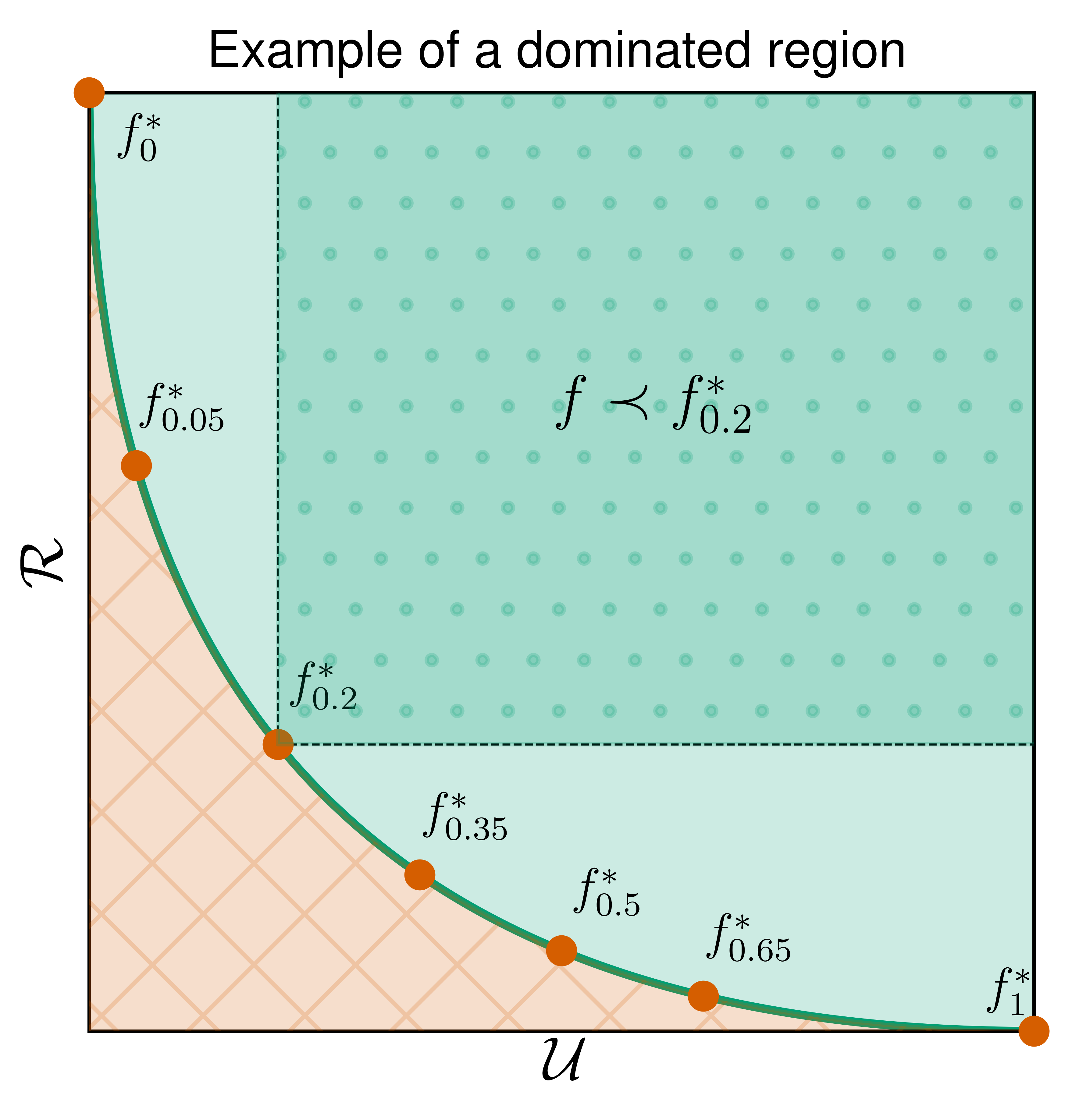
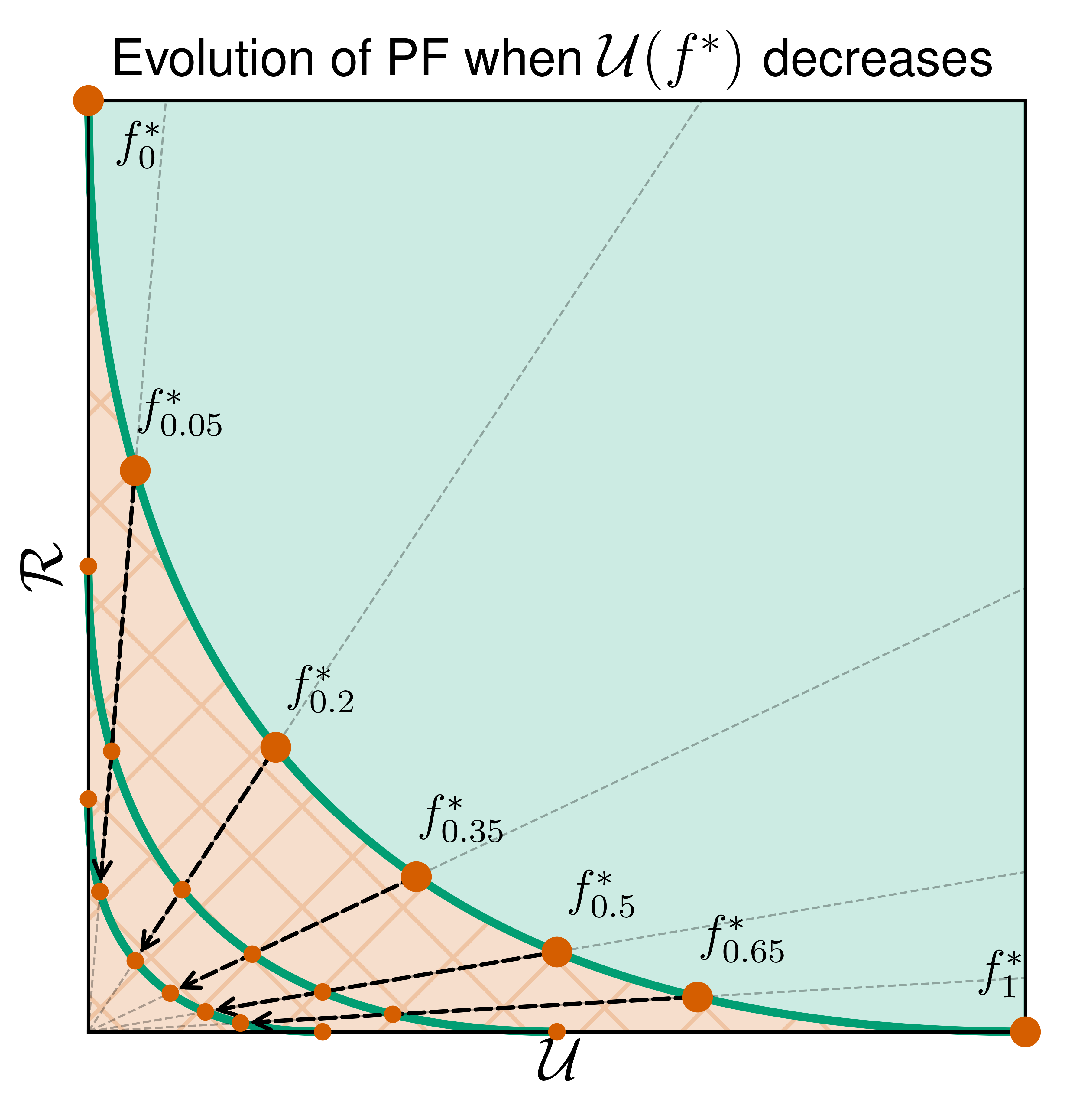
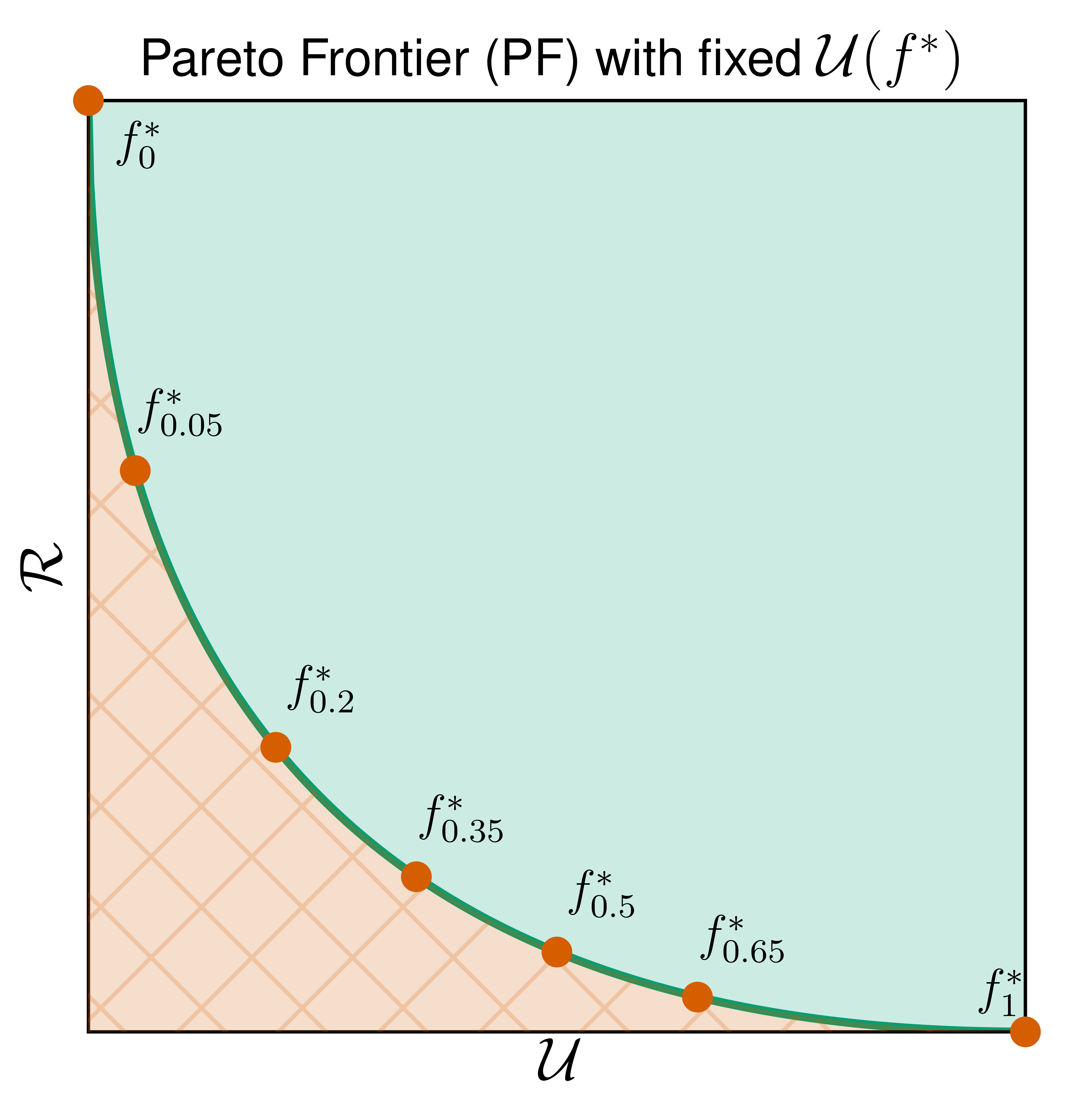
Figure 4: Illustration of Pareto frontiers and Pareto dominance. Left: Orange (hatched) part is not realisable by any prediction f𝑓f; Each point of green (not hatched) part is realizable by some prediction f𝑓f; The curve that separates the two is the Pareto frontier. Center: The darker green (dotted) rectangle in the upper right corner is the set of predictors dominated by f0.2subscriptsuperscript𝑓0.2f^{*}_{0.2}. Right: Evolution of the Pareto frontier when 𝒰(f)𝒰superscript𝑓\mathcal{U}(f^{*}) decreases.

Even though the parameter α[0,1]𝛼01\alpha\in[0,1] has a clear interpretation in our framework, one still might have to figure out which α𝛼\alpha to pick in practice. The ultimate theoretical goal is to find a prediction f𝑓f which simultaneously minimizes the risk \mathcal{R} and the unfairness 𝒰𝒰\mathcal{U}. Yet, unless fsuperscript𝑓f^{*} satisfies 𝒰(f)=0𝒰superscript𝑓0\mathcal{U}(f^{*})=0, this goal is unreachable and some trade-offs must be examined. A standard approach to study such multi-criteria optimization problems is via the notion of Pareto dominance and Pareto efficiency (Osborne and Rubinstein, 1994). In words, the idea of Pareto analysis is to restrict the attention of a practitioner to some set of “good” predictors, termed Pareto frontier of the multi-criteria optimization problem, instead of considering all possible predictions. In this section, we show that the set of oracle α𝛼\alpha-RI {fα}α[0,1]subscriptsubscriptsuperscript𝑓𝛼𝛼01\{f^{*}_{\alpha}\}_{\alpha\in[0,1]} is the Pareto frontier of the multi-criteria minimization problem with target functions f(f)maps-to𝑓𝑓f\mapsto\mathcal{R}(f) and f𝒰(f)maps-to𝑓𝒰𝑓f\mapsto\mathcal{U}(f).

Let us first introduce the terminology of the Pareto analysis specified for our setup. We say that a prediction f𝑓f Pareto dominates a prediction fsuperscript𝑓f^{\prime} if one of the following holds

  • (f)(f)𝑓superscript𝑓\mathcal{R}(f)\leq\mathcal{R}(f^{\prime}) and 𝒰(f)<𝒰(f)𝒰𝑓𝒰superscript𝑓\mathcal{U}(f)<\mathcal{U}(f^{\prime});

  • (f)<(f)𝑓superscript𝑓\mathcal{R}(f)<\mathcal{R}(f^{\prime}) and 𝒰(f)𝒰(f)𝒰𝑓𝒰superscript𝑓\mathcal{U}(f)\leq\mathcal{U}(f^{\prime}).

To denote the fact that fsuperscript𝑓f^{\prime} is dominated by f𝑓f we write ffprecedessuperscript𝑓𝑓f^{\prime}\prec f. Moreover, we say that fsuperscript𝑓f^{\prime} and f𝑓f are comparable if either ffprecedessuperscript𝑓𝑓f^{\prime}\prec f or ffprecedes𝑓superscript𝑓f\prec f^{\prime}. Intuitively, whenever ffprecedessuperscript𝑓𝑓f^{\prime}\prec f, the prediction f𝑓f is strictly preferable, since it is at least as good as fsuperscript𝑓f^{\prime} for both criteria and it is strictly better for at least one of them.

Note that not every two predictions are actually comparable, that is, the relation precedes\prec only defines a partial-order. It is a known fact that partially ordered sets can be partitioned into well-ordered chains, that is, every pair within the chain is comparable and the restriction of precedes\prec on this chain defines an order relation. In this set-theoretic terminology, a prediction f𝑓f is Pareto efficient if it is maximal within some chain in the sense of the partial order precedes\prec. In other words, a prediction f𝑓f is Pareto efficient if it is not dominated by any other prediction. The set of all Pareto efficient predictions is called the Pareto frontier and is denoted by PFPF\operatorname{PF}.

Note that it would be more accurate to say that fsuperscript𝑓f^{\prime} \mathbb{P}-Pareto dominates f𝑓f and fsuperscript𝑓f^{\prime} is \mathbb{P}-Pareto efficient, since the above definitions are acting on the level of population and they do depend on the underlying distribution. We omit this notation for simplicity. In general, an analytic description of the Pareto frontier PFPF\operatorname{PF} is not necessarily feasible. However, in our case, thanks to the analysis of the previous section, we can precisely describe the Pareto frontier of this problem.

Proposition 4.6.

Let Assumption 2.1 be satisfied. Then, the Pareto frontier for the multi-criteria minimization problem with objective functions (f)𝑓\mathcal{R}(f) and 𝒰(f)𝒰𝑓\mathcal{U}(f) is given by {fα}α[0,1]subscriptsubscriptsuperscript𝑓𝛼𝛼01\{f^{*}_{\alpha}\}_{\alpha\in[0,1]}.

Proof.

On the one hand, by definition of fαsubscriptsuperscript𝑓𝛼f^{*}_{\alpha} it holds that {fα}α[0,1]PFsubscriptsubscriptsuperscript𝑓𝛼𝛼01PF\{f^{*}_{\alpha}\}_{\alpha\in[0,1]}\subset\operatorname{PF}. On the other hand, let fPF𝑓PFf\in\operatorname{PF} with 𝒰(f)0𝒰𝑓0\mathcal{U}(f)\neq 0 and let αf:=𝒰(f)/𝒰(f)assignsubscript𝛼𝑓𝒰𝑓𝒰superscript𝑓\alpha_{f}\vcentcolon=\mathcal{U}(f)/\mathcal{U}(f^{*}). Then by the definition of αfsubscript𝛼𝑓\alpha_{f} it holds that 𝒰(f)=αf𝒰(f)𝒰𝑓subscript𝛼𝑓𝒰superscript𝑓\mathcal{U}(f)=\alpha_{f}\,\mathcal{U}(f^{*}). Furthermore, by definition of fαfsubscriptsuperscript𝑓subscript𝛼𝑓f^{*}_{\alpha_{f}} it holds that (fαf)(f)subscriptsuperscript𝑓subscript𝛼𝑓𝑓\mathcal{R}(f^{*}_{\alpha_{f}})\leq\mathcal{R}(f) and by Lemma 4.5 it holds that 𝒰(fαf)=αf𝒰(f)𝒰subscriptsuperscript𝑓subscript𝛼𝑓subscript𝛼𝑓𝒰superscript𝑓\mathcal{U}(f^{*}_{\alpha_{f}})=\alpha_{f}\,\mathcal{U}(f^{*}). Finally, since f𝑓f is Pareto efficient it holds that (f)(fαf)𝑓subscriptsuperscript𝑓subscript𝛼𝑓\mathcal{R}(f)\leq\mathcal{R}(f^{*}_{\alpha_{f}}). If fPF𝑓PFf\in\operatorname{PF} is such that 𝒰(f)=0𝒰𝑓0\mathcal{U}(f)=0, then it is as good as f0subscriptsuperscript𝑓0f^{*}_{0} in the sense of Pareto. The proof is concluded555To be more precise, one needs to introduce the equivalence relation similar-to\sim defined as ffsimilar-to𝑓superscript𝑓f\sim f^{\prime} iff (f)=(f)𝑓superscript𝑓\mathcal{R}(f)=\mathcal{R}(f^{\prime}) and 𝒰(f)=𝒰(f)𝒰𝑓𝒰superscript𝑓\mathcal{U}(f)=\mathcal{U}(f^{\prime}) and to perform the exact same proof on the quotient space. For the sake of presentation we omit this benign technicality.. ∎

Note that any predictor f𝑓f defines a point (𝒰(f),(f))𝒰𝑓𝑓(\mathcal{U}(f),\mathcal{R}(f)) in the coordinate system (𝒰,)𝒰(\mathcal{U},\mathcal{R}). The left plot of Figure 4 illustrates the Pareto frontier and those values of (𝒰,)𝒰(\mathcal{U},\mathcal{R}) that are attainable by some prediction f𝑓f. We remark that the convexity of the Pareto frontiers curve is due to the specific trade-off provided by the parameter α𝛼\alpha. For a general multi-criteria optimization problem this convexity is not ensured. The right plot of Figure 4 demonstrates the evolution of the Pareto frontier when 𝒰(f)𝒰superscript𝑓\mathcal{U}(f^{*}) decreases.

Finally, Proposition 4.6 provides simple practical guidelines for the study of the trade-off given by α𝛼\alpha. Note that since thanks to Lemma 4.5 it holds that (f0)=𝒰(f)subscriptsuperscript𝑓0𝒰superscript𝑓\mathcal{R}(f^{*}_{0})=\mathcal{U}(f^{*}) and 𝒰(f1)=𝒰(f)𝒰subscriptsuperscript𝑓1𝒰superscript𝑓\mathcal{U}(f^{*}_{1})=\mathcal{U}(f^{*}), then the practitioner needs to estimate only one quantity 𝒰(f)𝒰superscript𝑓\mathcal{U}(f^{*}) and trace the curve of Pareto frontier in order to establish the desired trade-off for the problem at hand.

4.5 Relation with fairness regularized problem

In this section we present one of the possible applications of the Pareto interpretation of the α𝛼\alpha-relative improvements. For each λ0𝜆0\lambda\geq 0, define (un)fairness regularized minimizer as

f,λargminf:p×[K]{(f)+λ𝒰(f)}.superscript𝑓𝜆subscriptargmin:𝑓superscript𝑝delimited-[]𝐾𝑓𝜆𝒰𝑓\displaystyle f^{*,\lambda}\in\operatorname*{arg\,min}_{f:\mathbb{R}^{p}\times[K]\to\mathbb{R}}\left\{\mathcal{R}(f)+\lambda\cdot\mathcal{U}(f)\right\}\enspace.

Note that the level sets of f(f)+λ𝒰(f)maps-to𝑓𝑓𝜆𝒰𝑓f\mapsto\mathcal{R}(f)+\lambda\cdot\mathcal{U}(f) induce an affine function in the coordinates (,𝒰)𝒰(\mathcal{R},\mathcal{U}). This simple observation allows to establish the connection between minimizers of the penalized objective and α𝛼\alpha-relative improvements—minimizers of the constrained problem.

Proposition 4.7.

Let Assumption 2.1 be satisfied. Then, for any λ0𝜆0\lambda\geq 0 it holds that

f,λfα(λ)withα(λ)=(1+λ)2.formulae-sequencesuperscript𝑓𝜆subscriptsuperscript𝑓𝛼𝜆with𝛼𝜆superscript1𝜆2\displaystyle f^{*,\lambda}\equiv f^{*}_{\alpha(\lambda)}\qquad\text{with}\qquad\alpha(\lambda)={(1+\lambda)^{-2}}\enspace.

As a sanity check, we observe that for λ=0𝜆0\lambda=0 we recover the Bayes optimal prediction ff1f,0superscript𝑓subscriptsuperscript𝑓1superscript𝑓0f^{*}\equiv f^{*}_{1}\equiv f^{*,0} and with λ𝜆\lambda approaching ++\infty, we obtain the expression for the fair optimal prediction f,+f0superscript𝑓subscriptsuperscript𝑓0f^{*,+\infty}\equiv f^{*}_{0}.

5 Minimax setup

While the previous section was dealing with the general framework on the population level, the goal of this section is to put forward a minimax setup for the statistical problem of regression with the introduced fairness constraints.

Let (𝑿1,S1,Y1),,(𝑿n,Sn,Yn)subscript𝑿1subscript𝑆1subscript𝑌1subscript𝑿𝑛subscript𝑆𝑛subscript𝑌𝑛(\boldsymbol{X}_{1},S_{1},Y_{1}),\ldots,(\boldsymbol{X}_{n},S_{n},Y_{n}) be i.i.d. sample with joint distribution 𝐏(f,𝜽)subscript𝐏superscript𝑓𝜽\mathbf{P}_{(f^{*},\boldsymbol{\theta})}, where the pair (f,𝜽)×Θsuperscript𝑓𝜽Θ(f^{*},\boldsymbol{\theta})\in\mathcal{F}\times\Theta for some class \mathcal{F} and ΘΘ\Theta. In this notation fsuperscript𝑓f^{*} is the regression function and 𝜽𝜽\boldsymbol{\theta} is a nuisance parameter. For example \mathcal{F} can be the set of all affine or Lipschitz continuous functions and ΘΘ\Theta defines additional assumptions on the model in Eq. (1) (see Section 6 for a concrete example). For a given fairness parameter α[0,1]𝛼01\alpha\in[0,1] and a given confidence parameter t>0𝑡0t>0, the goal of the statistician is to construct an estimator666As usual, an estimator f^^𝑓\hat{f} is a measurable mapping of data to the space of predictions. f^^𝑓\hat{f}, which simultaneously satisfies the following two properties

  1. 1.

    Uniform fairness guarantee:

    (f,𝜽)×Θ𝐏(f,𝜽)(𝒰(f^)α𝒰(f))1t,formulae-sequencefor-allsuperscript𝑓𝜽Θsubscript𝐏superscript𝑓𝜽𝒰^𝑓𝛼𝒰superscript𝑓1𝑡\displaystyle\forall(f^{*},\boldsymbol{\theta})\in\mathcal{F}\times\Theta\quad\mathbf{P}_{(f^{*},\boldsymbol{\theta})}\left(\mathcal{U}(\hat{f})\leq\alpha\,\mathcal{U}(f^{*})\right)\geq 1-t\enspace, (8)
  2. 2.

    Uniform risk guarantee:

    (f,𝜽)×Θ𝐏(f,𝜽)((f^)rn,α,f(,Θ,t))1t.formulae-sequencefor-allsuperscript𝑓𝜽Θsubscript𝐏superscript𝑓𝜽^𝑓subscript𝑟𝑛𝛼superscript𝑓Θ𝑡1𝑡\displaystyle\forall(f^{*},\boldsymbol{\theta})\in\mathcal{F}\times\Theta\quad\mathbf{P}_{(f^{*},\boldsymbol{\theta})}\left(\mathcal{R}(\hat{f})\leq r_{n,\alpha,f^{*}}(\mathcal{F},\Theta,t)\right)\geq 1-t\enspace. (9)

Eq. (8) states that the constructed estimator satisfies the fairness requirement with high probability uniformly over the class ×ΘΘ\mathcal{F}\times\Theta. Meanwhile, in Eq. (9) we seek for the smallest rate rn,α,f(,Θ,t)subscript𝑟𝑛𝛼superscript𝑓Θ𝑡r_{n,\alpha,f^{*}}(\mathcal{F},\Theta,t) to quantify the statistical price of being α𝛼\alpha-relatively fair. Note that rn,α,f(,Θ,t)subscript𝑟𝑛𝛼superscript𝑓Θ𝑡r_{n,\alpha,f^{*}}(\mathcal{F},\Theta,t) depends explicitly on fsuperscript𝑓f^{*}. This is explained by the fact that the fairness of f^^𝑓\hat{f} is measured relatively to fsuperscript𝑓f^{*}, hence the price of this constraint also depends on the initial unfairness level of the regression function fsuperscript𝑓f^{*}.

The actual construction of the estimator f^^𝑓\hat{f} is problem dependent and the proving that it satisfies Eqs. (8)–(9) requires a careful case-by-case study. In Section 6 we provide an example of such analysis for a simple statistical model of linear regression with systematic group-dependent bias.

5.1 Generic lower bound

While the upper bounds of Eqs. (8)–(9) require a problem dependent analysis, a general problem dependent lower bound can be derived. In this section we develop such lower bound. Let us first introduce some useful definitions.

Assumption 5.1 (Unconstrained rate).

For a fixed confidence level t(0,1)𝑡01t\in(0,1) and a class (,Θ)Θ(\mathcal{F},\Theta), there exists a positive sequence δn(,Θ,t)subscript𝛿𝑛Θ𝑡\delta_{n}(\mathcal{F},\Theta,t) such that

inff^sup(f,𝜽)×Θ𝐏(f,𝜽)((f^)δn(,Θ,t))t,subscriptinfimum^𝑓subscriptsupremumsuperscript𝑓𝜽Θsubscript𝐏superscript𝑓𝜽^𝑓subscript𝛿𝑛Θ𝑡𝑡\displaystyle\inf_{\hat{f}}\sup_{(f^{*},\boldsymbol{\theta})\in\mathcal{F}\times\Theta}\mathbf{P}_{(f^{*},\boldsymbol{\theta})}\left(\mathcal{R}(\hat{f})\geq\delta_{n}(\mathcal{F},\Theta,t)\right)\geq t\enspace,

where the infimum is taken over all estimators.

Assumption 5.1 can be used with any sequence δn(,Θ,t)subscript𝛿𝑛Θ𝑡\delta_{n}(\mathcal{F},\Theta,t), however, we implicitly assume that δn(,Θ,t)subscript𝛿𝑛Θ𝑡\delta_{n}(\mathcal{F},\Theta,t) corresponds to the minimax optimal rate of estimation of fsuperscript𝑓f^{*} by any estimator (without constraints) in expected squared loss.

Definition 5.2 (Valid estimators).

For some α[0,1]𝛼01\alpha\in[0,1] and confidence level t(0,1)superscript𝑡01t^{\prime}\in(0,1) we say that an estimator f^^𝑓\hat{f} is (α,t)𝛼superscript𝑡(\alpha,t^{\prime})-valid w.r.t. the class (,Θ)Θ(\mathcal{F},\Theta) if

inf(f,𝜽)×Θ𝐏(f,𝜽)(𝒰(f^)α𝒰(f))1t.subscriptinfimumsuperscript𝑓𝜽Θsubscript𝐏superscript𝑓𝜽𝒰^𝑓𝛼𝒰superscript𝑓1superscript𝑡\displaystyle\inf_{{(f^{*},\boldsymbol{\theta})}\in\mathcal{F}\times\Theta}\mathbf{P}_{(f^{*},\boldsymbol{\theta})}\left(\mathcal{U}(\hat{f})\leq\alpha\,\mathcal{U}({f^{*}})\right)\geq 1-t^{\prime}\enspace.

The set of all (α,t)𝛼superscript𝑡(\alpha,t^{\prime})-valid estimators w.r.t. the class (,Θ)Θ(\mathcal{F},\Theta) is denoted by ^(α,t)subscript^𝛼superscript𝑡\widehat{\mathcal{F}}_{(\alpha,t^{\prime})}.

Definition 5.2 characterizes estimators which satisfy the α𝛼\alpha-RI constraint at least with constant probability uniformly over the class (,Θ)Θ(\mathcal{F},\Theta).

Equipped with Assumption 5.1 and Definition 5.2 we are in position to state the main result of this section, which establishes the statistical risk-fairness trade-off. As we will see in Section 6, supported by appropriate upper bounds, Theorem 5.3 yields optimal rates of convergence up to a multiplicative factor.

Theorem 5.3.

Let Assumption 2.1 be satisfied. Let δn(,Θ,t)subscript𝛿𝑛Θ𝑡\delta_{n}(\mathcal{F},\Theta,t) be a sequence that satisfies Assumption 5.1. Then

inff^^(α,t)sup(f,𝜽)×Θ𝐏(f,𝜽)(1/2(f^)δn1/2(,Θ,t)(1α)𝒰1/2(f))t(1t).subscriptinfimum^𝑓subscript^𝛼superscript𝑡subscriptsupremumsuperscript𝑓𝜽Θsubscript𝐏superscript𝑓𝜽superscript12^𝑓superscriptsubscript𝛿𝑛12Θ𝑡1𝛼superscript𝒰12superscript𝑓𝑡1superscript𝑡\displaystyle\inf_{\hat{f}\in\widehat{\mathcal{F}}_{(\alpha,t^{\prime})}}\sup_{{(f^{*},\boldsymbol{\theta})}\in\mathcal{F}\times\Theta}\mathbf{P}_{{(f^{*},\boldsymbol{\theta})}}\left(\mathcal{R}^{\nicefrac{{1}}{{2}}}(\hat{f})\geq\delta_{n}^{\nicefrac{{1}}{{2}}}(\mathcal{F},\Theta,t)\vee(1{-}\sqrt{\alpha})\mathcal{U}^{\nicefrac{{1}}{{2}}}({f^{*}})\right)\geq t\wedge(1-t^{\prime})\enspace.

Drawing an analogy with Lemma 4.5, the two terms of the derived bound have natural interpretations: the first term δn(,Θ,t)subscript𝛿𝑛Θ𝑡\delta_{n}(\mathcal{F},\Theta,t) is the price of statistical estimation; the second term (1α)2𝒰(f)superscript1𝛼2𝒰superscript𝑓(1{-}\sqrt{\alpha})^{2}\mathcal{U}({f^{*}}) is the price of fairness. Consequently, the rate rn,α,f(,Θ,t)subscript𝑟𝑛𝛼superscript𝑓Θ𝑡r_{n,\alpha,f^{*}}(\mathcal{F},\Theta,t) in Eq. (9) is lower bounded (up to a multiplicative constant factor) by δn1/2(,Θ,t)(1α)𝒰1/2(f)superscriptsubscript𝛿𝑛12Θ𝑡1𝛼superscript𝒰12superscript𝑓\delta_{n}^{\nicefrac{{1}}{{2}}}(\mathcal{F},\Theta,t)\vee(1{-}\sqrt{\alpha})\mathcal{U}^{\nicefrac{{1}}{{2}}}({f^{*}}). The confidence parameter on the r.h.s. of the bound is t(1t)𝑡1superscript𝑡t\wedge(1-t^{\prime}). The reasonable choice of tsuperscript𝑡t^{\prime} is in the vicinity of zero, which corresponds to estimators satisfying the fairness constraint with high probability. Finally, observe that this bound is not conventional in the sense of classical statistics, where the bound would converge to zero with the growth of sample size. This behavior is not surprising, since the infimum is taken w.r.t. to (α,t)𝛼superscript𝑡(\alpha,t^{\prime})-valid estimators and not w.r.t. all possible estimators. One can draw an analogy of the obtained bound with recent results in robust statistics (Chen, Gao and Ren, 2016, 2018), where the minimax rate converges to a function of the proportion of outliers, which might be different from zero.

6 Application to linear model with systematic bias

Additional notation. We denote by 2\|\cdot\|_{2} and by n=(1/n)2\|\cdot\|_{n}=(\nicefrac{{1}}{{\sqrt{n}}})\|\cdot\|_{2} the Euclidean and the normalized Euclidean norm. The standard scalar product is denoted by ,\left\langle\cdot,\cdot\right\rangle. We denote by 𝟏psubscript1𝑝\boldsymbol{1}_{p} the vector of all ones of size p𝑝p. For square matrix 𝐀n×n,n1formulae-sequence𝐀superscript𝑛𝑛𝑛1\mathbf{A}\in\mathbb{R}^{n\times n},n\geq 1, we write 𝐀0succeeds𝐀0\mathbf{A}\succ 0 if 𝐀𝐀\mathbf{A} is symmetric positive-definite.

The goal of this part is to provide an example of a complete statistical analysis for a regression problem under the α𝛼\alpha-RI constraint. In particular, we show how to apply the plug-and-play results of Section 5.1 in order to derive minimax rate optimal bounds under the α𝛼\alpha-RI constraint. To this end we apply the developed theory to the following model of linear regression with systematic group-dependent bias

Y=𝑿,𝜷+bS+ξ,𝑌𝑿superscript𝜷superscriptsubscript𝑏𝑆𝜉\displaystyle Y=\left\langle\boldsymbol{X},\boldsymbol{\beta}^{*}\right\rangle+b_{S}^{*}+\xi\enspace, (10)

where 𝑿𝒩(𝟎,𝚺)similar-to𝑿𝒩0𝚺\boldsymbol{X}\sim\mathcal{N}(\boldsymbol{0},\mathbf{\Sigma}) is a feature vector independent from the sensitive attribute S𝑆S with 𝚺0succeeds𝚺0\mathbf{\Sigma}\succ 0; ξ𝒩(0,σ2)similar-to𝜉𝒩0superscript𝜎2\xi\sim\mathcal{N}({0},\sigma^{2}) is an additive independent noise; and the vector 𝒃=(b1,,bK)superscript𝒃superscriptsubscript𝑏1superscriptsubscript𝑏𝐾\boldsymbol{b}^{*}=(b_{1}^{*},\ldots,b_{K}^{*}) is the vector of systematic bias. We assume that the noise level σ𝜎\sigma is known to the statistician. Note that in this case the regression function fsuperscript𝑓f^{*} is given by the expression f(𝒙,s)=𝒙,𝜷+bssuperscript𝑓𝒙𝑠𝒙superscript𝜷superscriptsubscript𝑏𝑠f^{*}(\boldsymbol{x},s)=\left\langle\boldsymbol{x},\boldsymbol{\beta}^{*}\right\rangle+b_{s}^{*} and Assumption 2.1 is satisfied. We assume that the observations are

𝒀s=𝐗s𝜷+bs𝟏ns+𝝃s,s=1,,K,formulae-sequencesubscript𝒀𝑠subscript𝐗𝑠superscript𝜷superscriptsubscript𝑏𝑠subscript1subscript𝑛𝑠subscript𝝃𝑠𝑠1𝐾\displaystyle\boldsymbol{Y}_{s}=\mathbf{X}_{s}\boldsymbol{\beta}^{*}+b_{s}^{*}\boldsymbol{1}_{n_{s}}+\boldsymbol{\xi}_{s},\quad s=1,\ldots,K\enspace, (11)

with 𝒀s,𝝃snssubscript𝒀𝑠subscript𝝃𝑠superscriptsubscript𝑛𝑠\boldsymbol{Y}_{s},\boldsymbol{\xi}_{s}\in\mathbb{R}^{n_{s}}, 𝐗sns×psubscript𝐗𝑠superscriptsubscript𝑛𝑠𝑝\mathbf{X}_{s}\in\mathbb{R}^{n_{s}\times p}, and 𝟏nssubscript1subscript𝑛𝑠\boldsymbol{1}_{n_{s}} is the vector of all ones of size nssubscript𝑛𝑠n_{s}. The rows of 𝐗ssubscript𝐗𝑠\mathbf{X}_{s} are i.i.d. realization of 𝑿𝑿\boldsymbol{X}, the components of 𝝃ssubscript𝝃𝑠\boldsymbol{\xi}_{s} are i.i.d. from 𝒩(0,σ2)𝒩0superscript𝜎2\mathcal{N}(0,\sigma^{2}). Additionally, we set n=n1++nK𝑛subscript𝑛1subscript𝑛𝐾n=n_{1}+\ldots+n_{K} and ws=ns/nsubscript𝑤𝑠subscript𝑛𝑠𝑛w_{s}=\nicefrac{{n_{s}}}{{n}}. The risk of f:p×[K]:𝑓superscript𝑝delimited-[]𝐾f:\mathbb{R}^{p}\times[K]\to\mathbb{R} is then defined as

(f)=s=1Kws𝔼(𝑿,𝜷+bsf(𝑿,s))2.𝑓superscriptsubscript𝑠1𝐾subscript𝑤𝑠𝔼superscript𝑿superscript𝜷superscriptsubscript𝑏𝑠𝑓𝑿𝑠2\displaystyle\mathcal{R}(f)=\sum_{s=1}^{K}w_{s}\mathbb{E}\left(\left\langle\boldsymbol{X},\boldsymbol{\beta}^{*}\right\rangle+b_{s}^{*}-f(\boldsymbol{X},s)\right)^{2}\enspace.
Remark 6.1.

We set ws=ns/nsubscript𝑤𝑠subscript𝑛𝑠𝑛w_{s}=\nicefrac{{n_{s}}}{{n}} instead of ws=(S=s)subscript𝑤𝑠𝑆𝑠w_{s}=\mathbb{P}(S=s) to simplify the presentation and proofs of the main results. Note that if S1,,Snsubscript𝑆1subscript𝑆𝑛S_{1},\ldots,S_{n} is an i.i.d. sample, then ns=i=1n𝕀{Si=s}subscript𝑛𝑠superscriptsubscript𝑖1𝑛𝕀subscript𝑆𝑖𝑠n_{s}=\sum_{i=1}^{n}\mathbb{I}{\left\{S_{i}=s\right\}} and 𝐄[ns/n]=(S=s)𝐄delimited-[]subscript𝑛𝑠𝑛𝑆𝑠\mathbf{E}[\nicefrac{{n_{s}}}{{n}}]=\mathbb{P}(S=s), that is our choice of weights essentially corresponds to the scenario of i.i.d. sampling of sensitive attribute.

Using the terminology of Section 5.1 the joint distribution of data sample 𝐏(f,𝜽)subscript𝐏superscript𝑓𝜽\mathbf{P}_{(f^{*},\boldsymbol{\theta})} is uniquely defined by (𝜷,𝒃)superscript𝜷superscript𝒃(\boldsymbol{\beta}^{*},\boldsymbol{b}^{*}) and (𝚺,σ)𝚺𝜎(\mathbf{\Sigma},\sigma). That is, (𝜷,𝒃)superscript𝜷superscript𝒃(\boldsymbol{\beta}^{*},\boldsymbol{b}^{*}) defines the regression function fsuperscript𝑓f^{*} and (𝚺,σ)𝚺𝜎(\mathbf{\Sigma},\sigma) is the nuisance parameter 𝜽𝜽\boldsymbol{\theta}. To simplify the notation we write 𝐏(𝜷,𝒃)subscript𝐏superscript𝜷superscript𝒃\mathbf{P}_{(\boldsymbol{\beta}^{*},\boldsymbol{b}^{*})} instead of 𝐏(𝜷,𝒃,𝚺,σ)subscript𝐏superscript𝜷superscript𝒃𝚺𝜎\mathbf{P}_{(\boldsymbol{\beta}^{*},\boldsymbol{b}^{*},\mathbf{\Sigma},\sigma)}.

The following result is the application of Proposition 4.1 to the model in Eq. (10).

Proposition 6.2.

For all α[0,1]𝛼01\alpha\in[0,1], the α𝛼\alpha-relative improvement of fsuperscript𝑓f^{*} is given for all (𝐱,s)p×[K]𝐱𝑠superscript𝑝delimited-[]𝐾(\boldsymbol{x},s)\in\mathbb{R}^{p}\times[K] by

fα(𝒙,s)=𝒙,𝜷+αbs+(1α)s=1Kwsbs.subscriptsuperscript𝑓𝛼𝒙𝑠𝒙superscript𝜷𝛼superscriptsubscript𝑏𝑠1𝛼superscriptsubscript𝑠1𝐾subscript𝑤𝑠superscriptsubscript𝑏𝑠\displaystyle f^{*}_{\alpha}(\boldsymbol{x},s)=\left\langle\boldsymbol{x},\boldsymbol{\beta}^{*}\right\rangle+\sqrt{\alpha}b_{s}^{*}+(1{-}\sqrt{\alpha})\sum_{s=1}^{K}w_{s}b_{s}^{*}\enspace.

In order to build an estimator f^^𝑓\hat{f}, which improves the fairness of fsuperscript𝑓f^{*}, while providing minimal risk among such predictions, we first estimate parameters of model in Eq. (10) using least-squares estimators

(𝜷^,𝒃^)argmin(𝜷,𝒃)p×Ks=1Kws𝒀s𝐗s𝜷bs𝟏nsns2.bold-^𝜷bold-^𝒃subscriptargmin𝜷𝒃superscript𝑝superscript𝐾superscriptsubscript𝑠1𝐾subscript𝑤𝑠superscriptsubscriptdelimited-∥∥subscript𝒀𝑠subscript𝐗𝑠𝜷subscript𝑏𝑠subscript1subscript𝑛𝑠subscript𝑛𝑠2\displaystyle({\boldsymbol{\hat{\beta}}},\boldsymbol{\hat{b}})\in\operatorname*{arg\,min}_{(\boldsymbol{\beta},\boldsymbol{b})\in\mathbb{R}^{p}\times\mathbb{R}^{K}}\sum_{s=1}^{K}w_{s}\left\lVert\boldsymbol{Y}_{s}-\mathbf{X}_{s}\boldsymbol{\beta}-b_{s}\boldsymbol{1}_{n_{s}}\right\rVert_{n_{s}}^{2}\enspace. (12)

Based on the above quantities we then define a family of linear estimators f^τsubscript^𝑓𝜏\hat{f}_{\tau} parametrized by τ[0,1]𝜏01\tau\in[0,1] as

f^τ(𝒙,s)=𝒙,𝜷^+τb^s+(1τ)s=1Kwsb^s,(𝒙,s)p×[K].formulae-sequencesubscript^𝑓𝜏𝒙𝑠𝒙bold-^𝜷𝜏subscript^𝑏𝑠1𝜏superscriptsubscript𝑠1𝐾subscript𝑤𝑠subscript^𝑏𝑠𝒙𝑠superscript𝑝delimited-[]𝐾\displaystyle\hat{f}_{\tau}(\boldsymbol{x},s)=\langle\boldsymbol{x},{\boldsymbol{\hat{\beta}}}\rangle+\sqrt{\tau}\hat{b}_{s}+(1{-}\sqrt{\tau})\sum_{s=1}^{K}w_{s}\hat{b}_{s}\,\,,\qquad(\boldsymbol{x},s)\in\mathbb{R}^{p}\times[K]\enspace. (13)

We would like to find a value of τ=τn(α)𝜏subscript𝜏𝑛𝛼\tau=\tau_{n}(\alpha) such that Eqs. (8)–(9) are satisfied. Note that the choice of τ=α𝜏𝛼\tau=\alpha would not yield the desired fairness guarantee stated in Eq. (8). As it will be shown later, τ𝜏\tau should be smaller than α𝛼\alpha, in order to account for finite sample effects and derive high confidence fairness guarantee. The next result shows that under the model in Eq. (10), the unfairness of f^τsubscript^𝑓𝜏\hat{f}_{\tau} can be computed in a data-driven manner, which is crucial for the consequent choice of τ𝜏\tau.

Lemma 6.3.

For any τ[0,1]𝜏01\tau\in[0,1], the unfairness of f^τsubscript^𝑓𝜏\hat{f}_{\tau} is given by

𝒰(f^τ)=τs=1Kws(b^ss=1Kwsb^s)2almost surely.𝒰subscript^𝑓𝜏𝜏superscriptsubscript𝑠1𝐾subscript𝑤𝑠superscriptsubscript^𝑏𝑠superscriptsubscriptsuperscript𝑠1𝐾subscript𝑤superscript𝑠subscript^𝑏superscript𝑠2almost surely\displaystyle\mathcal{U}(\hat{f}_{\tau})=\tau\sum_{s=1}^{K}w_{s}\left(\hat{b}_{s}-\sum_{s^{\prime}=1}^{K}w_{s^{\prime}}\hat{b}_{s^{\prime}}\right)^{2}\qquad\text{almost surely}\enspace.

Apart from being computable in practice, Lemma 6.3 provides an intuitive result that 𝒰(f^τ)𝒰subscript^𝑓𝜏\mathcal{U}(\hat{f}_{\tau}) is the variance of the bias term 𝒃^bold-^𝒃\boldsymbol{\hat{b}}.

6.1 Upper bound

Linear regression is one of the most well-studied problems of statistics (Nemirovski, 2000, Tsybakov, 2003, Györfi et al., 2006, Mourtada, 2019, Catoni, 2004, Hsu, Kakade and Zhang, 2012, Audibert and Catoni, 2011). In the context of fairness, linear regression is considered in (Calders et al., 2013, Berk et al., 2017, Donini et al., 2018), where the fairness constraint is formulated via the approximate equality of group-wise means. In this section we establish a statistical guarantee on the risk and fairness of f^τsubscript^𝑓𝜏\hat{f}_{\tau} for an appropriate data-driven choice of τ𝜏\tau. Our theoretical analysis in this part is inspired by that of Hsu, Kakade and Zhang (2012), who derived high probability bounds on least squares estimator for linear regression with random design.

The following rate plays a crucial rule in the analysis of this section

δn(p,K,t)=8(pn+Kn)+16(pn+Kn)tn+32tn.subscript𝛿𝑛𝑝𝐾𝑡8𝑝𝑛𝐾𝑛16𝑝𝑛𝐾𝑛𝑡𝑛32𝑡𝑛\displaystyle\delta_{n}(p,K,t)=8\left(\frac{p}{n}+\frac{K}{n}\right)+16\left(\sqrt{\frac{p}{n}}+\sqrt{\frac{K}{n}}\right)\sqrt{\frac{t}{n}}+\frac{32t}{n}\enspace.

Not taking into account the confidence parameter t>0𝑡0t>0, δn(p,K,t)(p+K)/nasymptotically-equalssubscript𝛿𝑛𝑝𝐾𝑡𝑝𝐾𝑛\delta_{n}(p,K,t)\asymp{(p+K)}/{n} up to a constant multiplicative factor, which as it is shown in Theorem 6.5 is the minimax optimal rate for the model in Eq. (10) without the fairness constraint.

Theorem 6.4 (Fairness and risk upper bound).

Define

τ^={α(1+σδn1/2(p,K,t)𝒰1/2(f^1)σδn1/2(p,K,t))2 if 𝒰1/2(f^1)>σδn1/2(p,K,t)0, otherwise.^𝜏cases𝛼superscript1𝜎subscriptsuperscript𝛿12𝑛𝑝𝐾𝑡superscript𝒰12subscript^𝑓1𝜎subscriptsuperscript𝛿12𝑛𝑝𝐾𝑡2 if superscript𝒰12subscript^𝑓1𝜎subscriptsuperscript𝛿12𝑛𝑝𝐾𝑡0 otherwise\displaystyle\hat{\tau}=\begin{cases}\alpha\left(1+\frac{\sigma{\delta^{\nicefrac{{1}}{{2}}}_{n}(p,K,t)}}{{\mathcal{U}^{\nicefrac{{1}}{{2}}}(\hat{f}_{1})}-\sigma{\delta^{\nicefrac{{1}}{{2}}}_{n}(p,K,t)}}\right)^{-2}&\text{ if }\quad{\mathcal{U}^{\nicefrac{{1}}{{2}}}(\hat{f}_{1})}>\sigma{\delta^{\nicefrac{{1}}{{2}}}_{n}(p,K,t)}\\ 0,&\text{ otherwise}\end{cases}\enspace.

Consider p,K,t0formulae-sequence𝑝𝐾𝑡0p,K\in\mathbb{N},t\geq 0 and define θ(p,K,t)=(4K+5t+6p)/(p+t)𝜃𝑝𝐾𝑡4𝐾5𝑡6𝑝𝑝𝑡\theta(p,K,t)=\nicefrac{{(4\sqrt{K}+5\sqrt{t}+6\sqrt{p})}}{{(\sqrt{p}+\sqrt{t})}}. Assume that n2(p+t)/(θ(p,K,t)θ2(p,K,t)3)𝑛2𝑝𝑡𝜃𝑝𝐾𝑡superscript𝜃2𝑝𝐾𝑡3\sqrt{n}\geq 2\nicefrac{{(\sqrt{p}+\sqrt{t})}}{{(\theta(p,K,t)-\sqrt{\theta^{2}(p,K,t)-3})}}. Then, for any α[0,1]𝛼01\alpha\in[0,1], with probability at least 14exp(t/2)14𝑡21-4\exp(-t/2) it holds that

𝒰(f^τ^)α𝒰(f)and1/2(f^τ^)2σ(1+α)δn1/2(p,K,t)+(1α)𝒰1/2(f).formulae-sequence𝒰subscript^𝑓^𝜏𝛼𝒰superscript𝑓andsuperscript12subscript^𝑓^𝜏2𝜎1𝛼subscriptsuperscript𝛿12𝑛𝑝𝐾𝑡1𝛼superscript𝒰12superscript𝑓\displaystyle\mathcal{U}(\hat{f}_{\hat{\tau}})\leq\alpha\,\mathcal{U}(f^{*})\quad\text{and}\quad\mathcal{R}^{\nicefrac{{1}}{{2}}}(\hat{f}_{\hat{\tau}})\leq 2\sigma(1{+}\sqrt{\alpha}){\delta^{\nicefrac{{1}}{{2}}}_{n}(p,K,t)}+(1{-}\sqrt{\alpha})\,\mathcal{U}^{\nicefrac{{1}}{{2}}}(f^{*})\enspace.

Theorem 6.4 simultaneously provides two results: first, it shows that the estimator f^τ^subscript^𝑓^𝜏\hat{f}_{\hat{\tau}} is (α,4et/2)𝛼4superscript𝑒𝑡2(\alpha,4e^{-t/2})-valid, that is, it satisfies the fairness constraint with high probability; second it provides the rate of convergence which consists of two parts. The first part of the rate, σδn1/2(p,K,t)𝜎superscriptsubscript𝛿𝑛12𝑝𝐾𝑡\sigma\delta_{n}^{\nicefrac{{1}}{{2}}}(p,K,t), is the price of statistical estimation of (𝜷,𝒃)superscript𝜷superscript𝒃(\boldsymbol{\beta}^{*},\boldsymbol{b}^{*}), while the second part, (1α)𝒰1/2(f)1𝛼superscript𝒰12superscript𝑓(1{-}\sqrt{\alpha})\mathcal{U}^{\nicefrac{{1}}{{2}}}(f^{*}), is the price one has to pay when introducing the α𝛼\alpha-RI fairness constraint. In order to achieve the fairness validity, we need to loosen the value of α𝛼\alpha to reflect the base level of unfairness, that is, τ^^𝜏\hat{\tau} is adjusted by 𝒰(f^1)𝒰subscript^𝑓1\mathcal{U}(\hat{f}_{1}). Let us point out that the bound of Theorem 6.4 slightly differs from the conditions required by Eqs. (8)–(9). In particular, it provides a joint guarantee on risk and fairness.

Let us remark that the previous result requires n𝑛n to be sufficiently large, similarly to the conditions in (Hsu, Kakade and Zhang, 2012, Audibert and Catoni, 2011). One can obtain a more explicit, but more restrictive bound on n𝑛n by finding sufficient conditions under which the assumption on n𝑛n is satisfied. For instance, rough computations show that it is sufficient to assume that n16K𝑛16𝐾\sqrt{n}\geq 16\sqrt{K} and n12.5(p+t)𝑛12.5𝑝𝑡\sqrt{n}\geq 12.5(\sqrt{p}+\sqrt{t}).

At last, we emphasize that the choice of τ^^𝜏\hat{\tau} requires the knowledge of the noise level σ𝜎\sigma, that is, this choice is not adaptive. However, our proof can effortlessly be extended to the case when only an upper bound σ¯¯𝜎\bar{\sigma} on the noise level σ𝜎\sigma is known. In this case σ𝜎\sigma should be replaced by σ¯¯𝜎\bar{\sigma} in the definition of τ^^𝜏\hat{\tau} and in the resulting rate. The question of adaptation to σ𝜎\sigma without any prior knowledge should be treated separately and is out of the scope of this work.
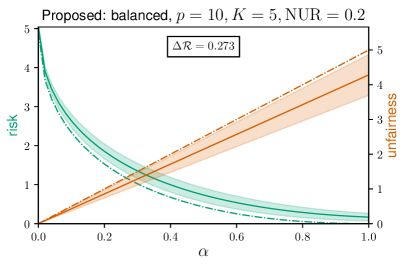
Refer to caption
Refer to caption
Refer to caption
Refer to caption
Figure 5: Dashed green and brown lines correspond to the risk and unfairness of fαsubscriptsuperscript𝑓𝛼f^{*}_{\alpha} respectively. Solid green and brown lines correspond to the average risk and unfairness of f^τ(α)subscript^𝑓𝜏𝛼\hat{f}_{\tau(\alpha)} and the shaded region shows three standard deviations over 505050 repetitions. On the left τ(α)=τ^𝜏𝛼^𝜏\tau(\alpha)=\hat{\tau} and on the risk τ(α)=α𝜏𝛼𝛼\tau(\alpha)=\alpha.

6.2 Lower bound

The goal of this section is to provide a lower bound, demonstrating that the result of Theorem 6.4 is minimax optimal up to a multiplicative constant factor. Recall that thanks to the general lower bound derived in Theorem 5.3 it is sufficient to prove a lower bound on the risk without constraining the set of possible estimators. Even though the problem of linear regression is well studied, to the best of our knowledge there is no known lower bound for the model in Eq. (10) which i) holds for the random design ii) is stated in probability iii) considers explicitly the confidence parameter t𝑡t. Next theorem establishes such lower bound.

Theorem 6.5.

For all n,p,K𝑛𝑝𝐾n,p,K\in\mathbb{N}, t0𝑡0t\geq 0, σ>0𝜎0\sigma>0 it holds that

inff^sup(𝜷,𝒃)p×K,𝚺0𝐏(𝜷,𝒃)((f^)σ2329n(p+K+32t)2)112et,subscriptinfimum^𝑓subscriptsupremumformulae-sequencesuperscript𝜷superscript𝒃superscript𝑝superscript𝐾succeeds𝚺0subscript𝐏superscript𝜷superscript𝒃^𝑓superscript𝜎23superscript29𝑛superscript𝑝𝐾32𝑡2112superscript𝑒𝑡\displaystyle\inf_{\hat{f}}\sup_{(\boldsymbol{\beta}^{*},\boldsymbol{b}^{*})\in\mathbb{R}^{p}\times\mathbb{R}^{K},\mathbf{\Sigma}\succ 0}\mathbf{P}_{(\boldsymbol{\beta}^{*},\boldsymbol{b}^{*})}\left(\mathcal{R}(\hat{f})\geq\frac{\sigma^{2}}{3\cdot 2^{9}n}(\sqrt{p+K}+\sqrt{32t})^{2}\right)\geq\frac{1}{12}e^{-t}\enspace,

where the infimum is taken w.r.t. all estimators.

The proof of Theorem 6.5 relies on standard information theoretic results. In particular, in order to prove optimal exponential concentration we follow similar strategy as that of Bellec (2017), Kerkyacharian et al. (2014) who derived optimal exponential concentrations in the context of density aggregation and binary classification. Theorem 6.5 combined with generic lower bound derived in Theorem 5.3 yields the following corollary.

Corollary 6.6.

Let δ¯n(p,K,t)=((p+K)/n+32t/n)2/(329)subscript¯𝛿𝑛𝑝𝐾𝑡superscript𝑝𝐾𝑛32𝑡𝑛23superscript29\bar{\delta}_{n}(p,K,t)=(\sqrt{\nicefrac{{(p+K)}}{{n}}}+\sqrt{\nicefrac{{32t}}{{n}}})^{2}/(3\cdot 2^{9}). For all n,p,K𝑛𝑝𝐾n,p,K\in\mathbb{N}, t0𝑡0t\geq 0, σ>0𝜎0\sigma>0, α[0,1]𝛼01\alpha\in[0,1] it holds for all t0𝑡0t\geq 0 and all t1et/12superscript𝑡1superscript𝑒𝑡12t^{\prime}\leq 1-\nicefrac{{e^{-t}}}{{12}} that

inff^^α,tsup(𝜷,𝒃)p×K,𝚺0𝐏(𝜷,𝒃)(1/2(f^)σδ¯n1/2(p,K,t)(1α)𝒰1/2(f))112et.subscriptinfimum^𝑓subscript^𝛼superscript𝑡subscriptsupremumformulae-sequencesuperscript𝜷superscript𝒃superscript𝑝superscript𝐾succeeds𝚺0subscript𝐏superscript𝜷superscript𝒃superscript12^𝑓𝜎subscriptsuperscript¯𝛿12𝑛𝑝𝐾𝑡1𝛼superscript𝒰12superscript𝑓112superscript𝑒𝑡\displaystyle\inf_{\hat{f}\in\widehat{\mathcal{F}}_{\alpha,t^{\prime}}}\sup_{(\boldsymbol{\beta}^{*},\boldsymbol{b}^{*})\in\mathbb{R}^{p}\times\mathbb{R}^{K},\mathbf{\Sigma}\succ 0}\mathbf{P}_{(\boldsymbol{\beta}^{*},\boldsymbol{b}^{*})}\left(\mathcal{R}^{\nicefrac{{1}}{{2}}}(\hat{f})\geq{\sigma}\bar{\delta}^{\nicefrac{{1}}{{2}}}_{n}(p,K,t)\vee(1{-}\sqrt{\alpha})\,\mathcal{U}^{\nicefrac{{1}}{{2}}}(f^{*})\right)\geq\frac{1}{12}e^{-t}\enspace.

Comparing the upper bound of Theorem 6.4 and the lower bound of Corollary 6.6 we conclude that the two obtained rates are the same up to a multiplicative constant factor. Hence confirming the tightness of the results derived in Section 5.1.

6.3 Simulation study

Refer to caption
Refer to caption
Refer to caption
Refer to caption
Figure 6: Dashed green and brown lines correspond to the risk and unfairness of fαsubscriptsuperscript𝑓𝛼f^{*}_{\alpha} respectively. Solid green and brown lines correspond to the average risk and unfairness of f^τ(α)subscript^𝑓𝜏𝛼\hat{f}_{\tau(\alpha)} and the shaded region shows three standard deviations over 505050 repetitions. On the left τ(α)=τ^𝜏𝛼^𝜏\tau(\alpha)=\hat{\tau} while on the right τ(α)=α𝜏𝛼𝛼\tau(\alpha)=\alpha.

In this section we perform simulation study to empirically validate our theoretical analysis777For our empirical validation and illustrations we have relied on the following python packages: scikit-learn (Pedregosa et al., 2011), numpy (Van Der Walt, Colbert and Varoquaux, 2011), matplotlib (Hunter, 2007), seaborn.. Before continuing let us discuss the notion of signal-to-unfairness ratio. Setting 𝜷=0superscript𝜷0\boldsymbol{\beta}^{*}=0 in the model (10), if the amplitudes of bssubscriptsuperscript𝑏𝑠b^{*}_{s} is much smaller than the noise level σ2superscript𝜎2\sigma^{2}, then the observations 𝒀ssubscript𝒀𝑠\boldsymbol{Y}_{s} are mainly composed of noise. While for the prediction problem it is not a problem, since our rates will scale with the noise level, it becomes important for the estimation of unfairness 𝒰(f)𝒰superscript𝑓\mathcal{U}(f^{*}). Motivated by this discussion, we define the noise-to-unfairness ratio as

NUR2:=σ2/𝒰(f).assignsuperscriptNUR2superscript𝜎2𝒰superscript𝑓\displaystyle\operatorname{NUR}^{2}\vcentcolon={\sigma^{2}}\big{/}{\mathcal{U}(f^{*})}\enspace.

The signal-to-unfairness ratio tells as how the level of unfairness compares to the noise level. The regime NUR1much-greater-thanNUR1\operatorname{NUR}\gg 1 means that the unfairness of the distributions is below the noise level, and it is statistically difficult to estimate it. In contrast, NUR1much-less-thanNUR1\operatorname{NUR}\ll 1 implies that the unfairness dominates the noise. Instead of varying 𝒰(f)𝒰superscript𝑓\mathcal{U}(f^{*}) and σ𝜎\sigma we fix σ𝜎\sigma and perform our study for different values of NURNUR\operatorname{NUR}.

We follow the following protocol. For some fixed K,n1,,nK,p,σ,NUR𝐾subscript𝑛1subscript𝑛𝐾𝑝𝜎NURK,n_{1},\ldots,n_{K},p,\sigma,\operatorname{NUR} we simulate the model in Eq. (11) with 𝚺=𝐈p𝚺subscript𝐈𝑝\mathbf{\Sigma}=\mathbf{I}_{p}. In all the experiments we set 𝜷=(1,,1)psuperscript𝜷superscript11topsuperscript𝑝\boldsymbol{\beta}^{*}=(1,\ldots,1)^{\top}\in\mathbb{R}^{p}. For 𝒃superscript𝒃\boldsymbol{b}^{*} we first define 𝒗=(1,1,1,1,)K𝒗superscript1111topsuperscript𝐾\boldsymbol{v}=(1,-1,1,-1,\ldots)^{\top}\in\mathbb{R}^{K} and set 𝒃=𝒗σ2/NURVarS(𝒗)superscript𝒃𝒗superscript𝜎2NURsubscriptVar𝑆𝒗\boldsymbol{b}^{*}=\boldsymbol{v}\sqrt{\nicefrac{{\sigma^{2}}}{{{\operatorname{NUR}\cdot\operatorname*{Var}_{S}(\boldsymbol{v})}}}}, where VarS(𝒗)subscriptVar𝑆𝒗\operatorname*{Var}_{S}(\boldsymbol{v}) is the variance of 𝒗𝒗\boldsymbol{v} with weights w1,,wKsubscript𝑤1subscript𝑤𝐾w_{1},\ldots,w_{K}. So that the unfairness of this model is exactly equal to σ2/NUR2superscript𝜎2superscriptNUR2\sigma^{2}/\operatorname{NUR}^{2}. On each simulation round of the model, we compute the estimator in Eq. (13) with two choices of parameter τ𝜏\tau:

  1. 1.

    Proposed: τ(α)=τ^𝜏𝛼^𝜏\tau(\alpha)=\hat{\tau} from Theorem 6.4;

  2. 2.

    Naive: τ(α)=α𝜏𝛼𝛼\tau(\alpha)=\alpha.

Remark 6.7.

While performing experiments we have noticed that setting τ^^𝜏\hat{\tau} with δn(p,K,t)subscript𝛿𝑛𝑝𝐾𝑡\delta_{n}(p,K,t) defined in Theorem 6.4 results in too pessimistic estimates in terms of unfairness, for this reason in all of our experiments we set δn(p,K,t)=(p/n)+(K/n)subscript𝛿𝑛𝑝𝐾𝑡𝑝𝑛𝐾𝑛\delta_{n}(p,K,t)=(\nicefrac{{p}}{{n}})+(\nicefrac{{K}}{{n}}), which is of the same order as that of Theorem 6.4.

Then, for each f^τ(α)subscript^𝑓𝜏𝛼\hat{f}_{\tau(\alpha)} we evaluate (f^τ(α))subscript^𝑓𝜏𝛼\mathcal{R}(\hat{f}_{\tau(\alpha)}) and 𝒰(f^τ(α))𝒰subscript^𝑓𝜏𝛼\mathcal{U}(\hat{f}_{\tau(\alpha)}). This procedure is repeated 505050 times, which results in 505050 values of (f^τ(α))subscript^𝑓𝜏𝛼\mathcal{R}(\hat{f}_{\tau(\alpha)}) and 𝒰(f^τ(α))𝒰subscript^𝑓𝜏𝛼\mathcal{U}(\hat{f}_{\tau(\alpha)}) for each α(0,1)𝛼01\alpha\in(0,1). For these 505050 values we compute mean and standard deviation. We considered p=10𝑝10p=10, K=5𝐾5K=5, σ=1𝜎1\sigma=1, and NUR{0.2,0.5,2}NUR0.20.52\operatorname{NUR}\in\{0.2,0.5,2\}. Furthermore, for the choice of n1,,nKsubscript𝑛1subscript𝑛𝐾n_{1},\ldots,n_{K} we study the following two regimes

  1. 1.

    Balanced: n1==n5=100subscript𝑛1subscript𝑛5100n_{1}=\ldots=n_{5}=100.

  2. 2.

    Unbalanced: n1=5,n2=45,n3=100,n4=100,n5=250formulae-sequencesubscript𝑛15formulae-sequencesubscript𝑛245formulae-sequencesubscript𝑛3100formulae-sequencesubscript𝑛4100subscript𝑛5250n_{1}=5,n_{2}=45,n_{3}=100,n_{4}=100,n_{5}=250.

The reason we consider two regimes is to confirm the theoretical findings of Theorem 6.4, which indicate that the rate is governed by n1++nKsubscript𝑛1subscript𝑛𝐾n_{1}+\ldots+n_{K} instead of the their individual values. Finally, for a given fairness parameter function ατ(α)maps-to𝛼𝜏𝛼\alpha\mapsto\tau(\alpha) we report cumulative risk increase over all α[0,1]𝛼01\alpha\in[0,1] defined as

Δ(τ):=01((f^τ(α))(fα))dα.assignΔ𝜏superscriptsubscript01subscript^𝑓𝜏𝛼subscriptsuperscript𝑓𝛼differential-d𝛼\displaystyle\Delta\mathcal{R}(\tau)\vcentcolon=\int_{0}^{1}\left(\mathcal{R}(\hat{f}_{\tau(\alpha)})-\mathcal{R}(f^{*}_{\alpha})\right)\,\,\mathrm{d}\alpha\enspace.

This quantity describes the cumulative risk loss of the rule τ(α)𝜏𝛼\tau(\alpha) across all the levels of fairness α𝛼\alpha compared to the best α𝛼\alpha-relative improvement fαsubscriptsuperscript𝑓𝛼f^{*}_{\alpha}.

On Figures 56 we draw the evolution of the risk and of the unfairness when α𝛼\alpha traverses the interval [0,1]01[0,1]. We also report Δ(τ)Δ𝜏\Delta\mathcal{R}(\tau) defined above. Inspecting the plots we can see that that the main disadvantage of the naive choice of τ=α𝜏𝛼\tau=\alpha is its poor fairness guarantee, that is, in almost half of the outcomes, the unfairness of f^αsubscript^𝑓𝛼\hat{f}_{\alpha} exceeded the prescribed value. In contrast, the proposed choice of τ(α)=τ^𝜏𝛼^𝜏\tau(\alpha)=\hat{\tau} consistently improves the unfairness of the regression function fsuperscript𝑓f^{*}, empirically validating our findings in Theorem 6.4. However, good fairness results come at the cost of consistently higher risk. One can also see that the effect of unbalanced distributions is negligible for the considered model (it only affects the variance of the result). This is explained by the definition of the risk, which weights the groups proportionally to their frequencies. Finally, observing the behavior of naive approach for NUR=0.2NUR0.2\operatorname{NUR}=0.2 and NUR=2NUR2\operatorname{NUR}=2 we note that in the latter case the unfairness of f^αsubscript^𝑓𝛼\hat{f}_{\alpha} starts to deviate from the true value (with consistently positive bias). Meanwhile, since the proposed choice τ(α)=τ^𝜏𝛼^𝜏\tau(\alpha)=\hat{\tau} is more conservative, the bias remains negative, that is, the unfairness of fsuperscript𝑓f^{*} is still improved.

7 Post-processing method without model

The previous section was concerned with illustrating the minimax setup, introduced in Section 5, with a concrete choice of parametric model. In practice, however, and especially for benchmark problems, parametric assumptions can hardly be verified; therefore, a more generic estimation algorithm, which does not rely on the modeling assumptions, is desirable.

In what follows, we propose a generic post-processing algorithm which can be applied on top of any black-box estimation procedure. Note that, due to the appealing structure of α𝛼\alpha-RI, we only need to estimate the two prediction functions: the Bayes rule fsuperscript𝑓f^{*} and the fair optimal f0subscriptsuperscript𝑓0f^{*}_{0}. Then, an estimator of fαsubscriptsuperscript𝑓𝛼f^{*}_{\alpha} can be built as a convex combination of the estimators of fsuperscript𝑓f^{*} and fsuperscript𝑓f^{*}. The literature on the estimation of the Bayes rule fsuperscript𝑓f^{*} is rather rich, thus, we only detail the estimation of f0subscriptsuperscript𝑓0f^{*}_{0}. Before proceeding, we introduce an additional bit of notation.

Additional notation. For any prediction function f:p×[K]:𝑓superscript𝑝delimited-[]𝐾f:\mathbb{R}^{p}\times[K]\to\mathbb{R}, any q[1,)𝑞1q\in[1,\infty), define

fqq:=s=1Kws𝔼[|f(𝑿,S)|qS=s]assignsuperscriptsubscriptdelimited-∥∥𝑓𝑞𝑞superscriptsubscript𝑠1𝐾subscript𝑤𝑠𝔼delimited-[]conditionalsuperscript𝑓𝑿𝑆𝑞𝑆𝑠\displaystyle\left\lVert f\right\rVert_{q}^{q}\vcentcolon=\sum_{s=1}^{K}w_{s}\mathbb{E}[|f(\boldsymbol{X},S)|^{q}\mid S=s]

and f:=s=1Kwsinf{b:(f(𝑿,S)<bS=s)=0}assignsubscriptdelimited-∥∥𝑓superscriptsubscript𝑠1𝐾subscript𝑤𝑠infimumconditional-set𝑏𝑓𝑿𝑆bra𝑏𝑆𝑠0\left\lVert f\right\rVert_{\infty}\vcentcolon=\sum_{s=1}^{K}w_{s}\inf\left\{b\in\mathbb{R}\,:\,\mathbb{P}(f(\boldsymbol{X},S)<b\mid S=s)=0\right\}.

7.1 The algorithm

For each sub-population s[K]𝑠delimited-[]𝐾s\in[K], let (𝑿1s,,𝑿2Nss)superscriptsubscript𝑿1𝑠superscriptsubscript𝑿2subscript𝑁𝑠𝑠(\boldsymbol{X}_{1}^{s},\ldots,\boldsymbol{X}_{2N_{s}}^{s}) be 2Ns2subscript𝑁𝑠2N_{s} i.i.d. feature vectors888For simplicity and without loss of generality, we assume that an even number of observations is available for every sensitive attribute. sampled from the distribution (𝑿S=s)conditional𝑿𝑆𝑠(\boldsymbol{X}\mid S=s), independently from (𝑿,S,Y)𝑿𝑆𝑌(\boldsymbol{X},S,Y) and from all other observations. Note that we explicitly allow ourselves to sample from each sensitive group separately. This is not restrictive, since an i.i.d. sample from \mathbb{P} can be converted into the considered sampling scheme by conditioning on the number of available observations from each group.

Let f:p×[K]:𝑓superscript𝑝delimited-[]𝐾f:\mathbb{R}^{p}\times[K]\to\mathbb{R} be a fixed prediction function. Our goal is to build a post-processing operator fΠ^(f):p×[K]:maps-to𝑓^Π𝑓superscript𝑝delimited-[]𝐾f\mapsto\hat{\Pi}(f):\mathbb{R}^{p}\times[K]\to\mathbb{R} such that the post-processing estimator Π^(f)^Π𝑓\hat{\Pi}(f) satisfies the Demographic Parity constraint and its closeness to f0subscriptsuperscript𝑓0f^{*}_{0} is controlled by that of f𝑓f to fsuperscript𝑓f^{*}. The rationale behind this goal is the representation of α𝛼\alpha -RI as a point-wise combination of fsuperscript𝑓f^{*} and f0subscriptsuperscript𝑓0f^{*}_{0}: if the considered function f𝑓f is a good estimator of fsuperscript𝑓f^{*} and Π^(f)^Π𝑓\hat{\Pi}(f) of f0subscriptsuperscript𝑓0f^{*}_{0}, then, as a trivial consequence of the triangle inequality, we can effectively estimate all of the {fα}α[0,1]subscriptsubscriptsuperscript𝑓𝛼𝛼01\{f^{*}_{\alpha}\}_{\alpha\in[0,1]}.

More formally, we want to build a (possibly randomized) operator Π^^Π\hat{\Pi} which satisfies, for every f:p×[K]:𝑓superscript𝑝delimited-[]𝐾f:\mathbb{R}^{p}\times[K]\to\mathbb{R}, q[1,+)𝑞1q\in[1,+\infty),

Law(Π^(f)(𝑿,S)S=s)=Law(Π^(f)(𝑿,S)S=s)s,s[K],formulae-sequenceLawconditional^Π𝑓𝑿𝑆𝑆𝑠Lawconditional^Π𝑓𝑿𝑆𝑆superscript𝑠for-all𝑠superscript𝑠delimited-[]𝐾\displaystyle\operatorname{Law}\left(\hat{\Pi}(f)(\boldsymbol{X},S)\mid S=s\right)=\operatorname{Law}\left(\hat{\Pi}(f)(\boldsymbol{X},S)\mid S=s^{\prime}\right)\qquad\forall s,s^{\prime}\in[K]\enspace,
𝐄Π^(f)f0qErrorq(f,f)+Remainder(N1,,NK),𝐄subscriptdelimited-∥∥^Π𝑓subscriptsuperscript𝑓0𝑞subscriptError𝑞𝑓superscript𝑓Remaindersubscript𝑁1subscript𝑁𝐾\displaystyle\mathbf{E}\left\lVert\hat{\Pi}(f)-f^{*}_{0}\right\rVert_{q}\leq\text{Error}_{q}(f,f^{*})+\text{Remainder}(N_{1},\ldots,N_{K})\enspace,

where Errorq(f,f)subscriptError𝑞𝑓superscript𝑓\text{Error}_{q}(f,f^{*}) represents the quality of the base estimator, which is supposed to be a good approximation of the Bayes rule fsuperscript𝑓f^{*}. Ideally, we want to have Errorq(f,f)=CffqsubscriptError𝑞𝑓superscript𝑓𝐶subscriptdelimited-∥∥𝑓superscript𝑓𝑞\text{Error}_{q}(f,f^{*})=C\cdot\left\lVert f-f^{*}\right\rVert_{q} for some C1𝐶1C\geq 1. We will achieve such a goal for q=1𝑞1q=1, while for q>1𝑞1q>1, the error term will be slightly different.

Remark 7.1.

Note that the first condition is stated with respect to the joint distribution of Π^(f)(𝐗,S)^Π𝑓𝐗𝑆\hat{\Pi}(f)(\boldsymbol{X},S), i.e., it involves all the randomness present in Π^(f)(𝐗,S)^Π𝑓𝐗𝑆\hat{\Pi}(f)(\boldsymbol{X},S).

Estimator construction. Let ζ,(ζis)i=1,,2Ns;s=1,,K𝜁subscriptsuperscriptsubscript𝜁𝑖𝑠formulae-sequence𝑖12subscript𝑁𝑠𝑠1𝐾\zeta,(\zeta_{i}^{s})_{i=1,\ldots,2N_{s};s=1,\ldots,K} be i.i.d. real valued random variables distributed uniformly on [σ,σ]𝜎𝜎[-\sigma,\sigma] for some σ>0𝜎0\sigma>0 to be specified. For each f:p×[K]:𝑓superscript𝑝delimited-[]𝐾f:\mathbb{R}^{p}\times[K]\to\mathbb{R}, each s[K]𝑠delimited-[]𝐾s\in[K] and i[2Ns]𝑖delimited-[]2subscript𝑁𝑠i\in[2N_{s}], define the following random variables

f~is:=f(𝑿is,s)+ζisandf~(𝒙,s):=f(𝒙,s)+ζ(𝒙,s)p×[K].formulae-sequenceassignsuperscriptsubscript~𝑓𝑖𝑠𝑓superscriptsubscript𝑿𝑖𝑠𝑠superscriptsubscript𝜁𝑖𝑠andformulae-sequenceassign~𝑓𝒙𝑠𝑓𝒙𝑠𝜁for-all𝒙𝑠superscript𝑝delimited-[]𝐾\displaystyle\tilde{f}_{i}^{s}\vcentcolon=f(\boldsymbol{X}_{i}^{s},s)+\zeta_{i}^{s}\quad\text{and}\quad\tilde{f}(\boldsymbol{x},s):=f(\boldsymbol{x},s)+\zeta\qquad\forall\,\,(\boldsymbol{x},s)\in\mathbb{R}^{p}\times[K]\enspace.

Using the above quantities, we build the following estimators: for all t𝑡t\in\mathbb{R}

F^1,νsf(t):=1Ns+1(i=1Ns𝕀{f~is<t}+Us(1+i=1Ns𝕀{f~is=t})),assignsubscript^𝐹1subscriptsuperscript𝜈𝑓𝑠𝑡1subscript𝑁𝑠1superscriptsubscript𝑖1subscript𝑁𝑠𝕀superscriptsubscript~𝑓𝑖𝑠𝑡superscript𝑈𝑠1superscriptsubscript𝑖1subscript𝑁𝑠𝕀superscriptsubscript~𝑓𝑖𝑠𝑡\displaystyle\hat{F}_{1,\nu^{f}_{s}}(t)\vcentcolon=\frac{1}{N_{s}{+}1}\left(\sum_{i=1}^{N_{s}}\mathbb{I}{\left\{\tilde{f}_{i}^{s}<t\right\}}+U^{s}\left(1{+}\sum_{i=1}^{N_{s}}\mathbb{I}{\left\{\tilde{f}_{i}^{s}=t\right\}}\right)\right)\enspace,
F^2,νsf(t):=1Nsi=Ns+12Ns𝕀{f~ist},assignsubscript^𝐹2subscriptsuperscript𝜈𝑓𝑠𝑡1subscript𝑁𝑠superscriptsubscript𝑖subscript𝑁𝑠12subscript𝑁𝑠𝕀superscriptsubscript~𝑓𝑖𝑠𝑡\displaystyle\hat{F}_{2,\nu^{f}_{s}}(t)\vcentcolon=\frac{1}{N_{s}}\sum_{i=N_{s}+1}^{2N_{s}}\mathbb{I}{\left\{\tilde{f}_{i}^{s}\leq t\right\}}\enspace,

where (Us)s[K]subscriptsuperscript𝑈𝑠𝑠delimited-[]𝐾(U^{s})_{s\in[K]} are i.i.d. random variables, distributed uniformly on [0,1]01[0,1] and independent from all the previously introduced random variables. Consequently, for each f:p×[K]:𝑓superscript𝑝delimited-[]𝐾f:\mathbb{R}^{p}\times[K]\to\mathbb{R} we define for all (𝒙,s)p×[K]𝒙𝑠superscript𝑝delimited-[]𝐾(\boldsymbol{x},s)\in\mathbb{R}^{p}\times[K]

Π^(f)(𝒙,s)=s=1KwsF^2,νsf1F^1,νsff~(𝒙,s).^Π𝑓𝒙𝑠superscriptsubscriptsuperscript𝑠1𝐾subscript𝑤superscript𝑠superscriptsubscript^𝐹2subscriptsuperscript𝜈𝑓superscript𝑠1subscript^𝐹1subscriptsuperscript𝜈𝑓𝑠~𝑓𝒙𝑠\displaystyle\hat{\Pi}(f)(\boldsymbol{x},s)=\sum_{s^{\prime}=1}^{K}w_{s^{\prime}}\hat{F}_{2,\nu^{f}_{s^{\prime}}}^{-1}\circ\hat{F}_{1,\nu^{f}_{s}}\circ\tilde{f}(\boldsymbol{x},s)\enspace. (14)

The form of our estimator was inspired by the explicit formula obtained for the fair optimal predictor f0superscriptsubscript𝑓0f_{0}^{*} (see Proposition 4.1). It can be seen as its empirical counterpart with additional randomization.

From now on our goal is to establish the desired guarantees on the operator Π^^Π\hat{\Pi}. A more in-depth study of this procedure is left for future works. We begin by providing an exact demographic parity guarantee.

Theorem 7.2 (Demographic parity guarantee).

For any f:p×[K]:𝑓superscript𝑝delimited-[]𝐾f:\mathbb{R}^{p}\times[K]\to\mathbb{R}, any joint distribution \mathbb{P} of (𝐗,S,Y)𝐗𝑆𝑌(\boldsymbol{X},S,Y) and any σ>0𝜎0\sigma>0, it holds that

Law(Π^(f)(𝑿,S)S=s)=Law(Π^(f)(𝑿,S)S=s)s,s[K].formulae-sequenceLawconditional^Π𝑓𝑿𝑆𝑆𝑠Lawconditional^Π𝑓𝑿𝑆𝑆superscript𝑠for-all𝑠superscript𝑠delimited-[]𝐾\displaystyle\operatorname{Law}\left(\hat{\Pi}(f)(\boldsymbol{X},S)\mid S=s\right)=\operatorname{Law}\left(\hat{\Pi}(f)(\boldsymbol{X},S)\mid S=s^{\prime}\right)\qquad\forall s,s^{\prime}\in[K]\enspace.

The above theorem may appear as “magical” at first sight as it holds under no assumption. To obtain such a result, we leverage distribution-free properties on rank and order statistics presented in Lemma LABEL:lem:inverse_with_noise in Appendix. This approach was inspired by the literature on conformal prediction (Vovk, Gammerman and Shafer, 2005, Lei and Wasserman, 2014, Lei et al., 2018, Barber et al., 2021) in which similar tools are used. Theorem 7.2 and the estimator in Eq. (14) improve upon the estimator of Chzhen et al. (2020a), for which only approximate fairness is established.

Since our fairness guarantee on its own is not necessarily informative (constant predictions trivially satisfy it), we complement it with a post-processing estimation bound to assess the predictive performance of our estimator. Unlike the previous result, which was assumption-free, we need an additional assumption stated below.

Assumption 7.3.

For all s[K]𝑠delimited-[]𝐾s\in[K], the measures νssuperscriptsubscript𝜈𝑠\nu_{s}^{*} are supported on an interval in \mathbb{R}, admit density w.r.t. Lebesgue measure which is lower and upper bounded by λ¯s>0subscript¯𝜆𝑠0\underline{\lambda}_{s}>0 and λ¯s>0subscript¯𝜆𝑠0\overline{\lambda}_{s}>0 respectively.

Note that the requirement of the existence of an upper-bounded density is not particularly restrictive. The most restrictive part of this assumption is the lower bound on this density. The reason we introduce it can be intuitively understood from asymptotic normality results on order statistics (see e.g., Van der Vaart, 2000, Section 21.2 and Corollary 21.5) which show that the limiting variance depends on the inverse density evaluated at the quantile that one wishes to estimate. In particular, it explodes when this density approaches zero. In our case, we actually need to estimate the whole quantile function (since f0subscriptsuperscript𝑓0f^{*}_{0} is based on it, see Prop. 4.1), hence we require that the density is uniformly lower bounded. It appears that the most important implication of the lower bounded density that we use is the λ¯s1superscriptsubscript¯𝜆𝑠1\underline{\lambda}_{s}^{-1}-Lipschitz continuity of the quantile function of νssubscriptsuperscript𝜈𝑠\nu^{*}_{s}. Due to this reason, it is certainly possible to relax the lower boundedness assumption by Hölder smoothness condition on the quantile function of νssubscriptsuperscript𝜈𝑠\nu^{*}_{s}. We leave this investigation for future works.

Theorem 7.4 (Estimation guarantee).

Let Assumptions 2.1 and 7.3 be satisfied, then for any base prediction rule f:p×[K]:𝑓superscript𝑝delimited-[]𝐾f:\mathbb{R}^{p}\times[K]\to\mathbb{R}, any σ(0,1)𝜎01\sigma\in(0,1) and any q[1,)𝑞1q\in[1,\infty), the proposed post-processing procedure satisfies

𝐄Π^(f)f0qC𝝀¯¯q(\displaystyle\mathbf{E}\lVert\hat{\Pi}(f)-f^{*}_{0}\rVert_{q}\leq C_{\overline{\underline{\boldsymbol{\lambda}}}}^{q}\bigg{(} ffq+min{ffq111/q+σ11/q,ff+σ}𝕀{q>1}subscriptdelimited-∥∥𝑓superscript𝑓𝑞superscriptsubscriptdelimited-∥∥𝑓superscript𝑓𝑞111𝑞superscript𝜎11𝑞subscriptdelimited-∥∥𝑓superscript𝑓𝜎𝕀𝑞1\displaystyle\left\lVert f-f^{*}\right\rVert_{q}{+}\min\left\{\left\lVert f-f^{*}\right\rVert_{q-1}^{1-\nicefrac{{1}}{{q}}}{+}\sigma^{1-\nicefrac{{1}}{{q}}},\,\left\lVert f-f^{*}\right\rVert_{\infty}{+}\sigma\right\}\mathbb{I}{\left\{q{>}1\right\}}
+{s=1KwsNs1/2}+{s=1KwsNsq/2}1/q+σ),\displaystyle+\left\{\sum_{s=1}^{K}w_{s}N_{s}^{-\nicefrac{{1}}{{2}}}\right\}+\left\{\sum_{s=1}^{K}w_{s}N_{s}^{-\nicefrac{{q}}{{2}}}\right\}^{\nicefrac{{1}}{{q}}}+\sigma\bigg{)}\enspace,

where C𝛌¯¯qsuperscriptsubscript𝐶¯¯𝛌𝑞C_{\overline{\underline{\boldsymbol{\lambda}}}}^{q} depends only on (λ¯s)s,(λ¯s)ssubscriptsubscript¯𝜆𝑠𝑠subscriptsubscript¯𝜆𝑠𝑠(\underline{\lambda}_{s})_{s},(\overline{\lambda}_{s})_{s} from Assumption 7.3 and q[1,)𝑞1q\in[1,\infty).

Note that for q=1𝑞1q=1 we get a “truly” post-processing guarantee—the quality of the post-processed prediction function in 1subscript1\ell_{1}-norm is controlled by the quality of the initial function in 1subscript1\ell_{1}-norm. For the case q>1𝑞1q>1, the bound slightly deteriorates and comprises two parts. One that involves a (q1)𝑞1(q{-}1)-norm to the power 11q11𝑞1-\tfrac{1}{q} and the other one involves a \infty-norm. Note that, following Stone (1977), it is always possible to build an estimator f𝑓f of fsuperscript𝑓f^{*} using an independent set of labeled data which is consistent in (q1)𝑞1(q{-}1)-norm. However, due to the presence of 11q11𝑞1-\tfrac{1}{q} in the exponent, the potential rate of convergence might be far from optimal. To this end, we included the term with \infty-norm. Indeed, under smoothness assumptions on fsuperscript𝑓f^{*} and extra conditions on 𝑿Ssubscriptconditional𝑿𝑆\mathbb{P}_{\boldsymbol{X}\mid S} it is possible to build estimators f𝑓f of fsuperscript𝑓f^{*} in \infty-norm only loosing an extra logarithmic factor (see e.g., Tsybakov, 2009) compared to the estimation in q<𝑞q<\infty norm. Furthermore we note that the constants in the above bound do not depend on the number of groups K𝐾K. The dependency on K𝐾K is implicit in the quality of estimation of fsuperscript𝑓f^{*} by f𝑓f and is explicit in the parametric part of the rate. As an example consider ws=(S=s)subscript𝑤𝑠𝑆𝑠w_{s}=\mathbb{P}(S=s), Ns=N(S=s)subscript𝑁𝑠𝑁𝑆𝑠N_{s}=N\cdot\mathbb{P}(S=s), and q=1𝑞1q=1. In that case the remainder term can be bounded by K/N𝐾𝑁\sqrt{\nicefrac{{K}}{{N}}}—the standard parametric rate.

8 Empirical study on real data

In this section we perform empirical study on the Communities and Crime dataset from UCI Machine Learning Repository999Data source: https://archive.ics.uci.edu/ml/datasets/communities+and+crime. We study the post-processing procedure described in Eq. (14) as well as the estimator from Eq. (13) that we designed in the context of linear regression with systematic bias in Section 6 (we refer to the latter estimator as BLS). The post-processing algorithm in Eq. (14) relies on some base estimator f𝑓f and we set f^α:=αf+(1α)Π^(f)assignsubscript^𝑓𝛼𝛼𝑓1𝛼^Π𝑓\hat{f}_{\alpha}\vcentcolon=\sqrt{\alpha}f+(1-\sqrt{\alpha})\hat{\Pi}(f). That is, for α=1𝛼1\alpha=1 we recover f^αfsubscript^𝑓𝛼𝑓\hat{f}_{\alpha}\equiv f—the base estimator itself. Thus, the BLS and each base estimator + post-processing induce a family of estimators parametrized by α[0,1]𝛼01\alpha\in[0,1]. In what follows we study these families of estimators.

8.1 Statistics about predictions

We split the dataset 𝒟𝒟\mathcal{D} into three disjoint parts: 𝒟trainsubscript𝒟train\mathcal{D}_{\operatorname{train}}, 𝒟unlabsubscript𝒟unlab\mathcal{D}_{\operatorname*{unlab}}, and 𝒟testsubscript𝒟test\mathcal{D}_{\operatorname{test}} (of sizes 50%,30%,20%percent50percent30percent2050\%,30\%,20\% respectively). The first, 𝒟trainsubscript𝒟train\mathcal{D}_{\operatorname{train}}, is used to fit an initial estimator f𝑓f of fsuperscript𝑓f^{*}; the second, 𝒟unlabsubscript𝒟unlab\mathcal{D}_{\operatorname*{unlab}}, is used to perform the post-processing Π^(f)^Π𝑓\hat{\Pi}(f) described in Eq. (14) (we set σ=106𝜎superscript106\sigma=10^{-6}); the last, 𝒟testsubscript𝒟test\mathcal{D}_{\operatorname{test}}, is used to compute various statistics related to the performance and fairness of estimators. For the estimator from Section 6 we use both 𝒟trainsubscript𝒟train\mathcal{D}_{\operatorname{train}} for the train, since it is a one-shot estimator, which does not require data splitting.

Let 𝒘ΔK1𝒘superscriptΔ𝐾1\boldsymbol{w}\in\Delta^{K-1} be a weight vector. For any predictor f:p×[K]:𝑓superscript𝑝delimited-[]𝐾f:\mathbb{R}^{p}\times[K]\rightarrow\mathbb{R}, we measure its performance with weighted mean-squared error on the test data

MSE^(f)=s=1Kws𝔼^[(Yf(𝑿,S))2S=s],^MSE𝑓superscriptsubscript𝑠1𝐾subscript𝑤𝑠^𝔼delimited-[]conditionalsuperscript𝑌𝑓𝑿𝑆2𝑆𝑠\displaystyle\widehat{\operatorname*{MSE}}(f)=\sum_{s=1}^{K}w_{s}\hat{\mathbb{E}}\left[(Y-f(\boldsymbol{X},S))^{2}\mid S=s\right]\enspace,

where 𝔼^^𝔼\hat{\mathbb{E}} is evaluated on 𝒟testsubscript𝒟test\mathcal{D}_{\operatorname{test}}. The unfairness estimator (see Appendix G for details on this estimator) of f:p×[K]:𝑓superscript𝑝delimited-[]𝐾f:\mathbb{R}^{p}\times[K]\rightarrow\mathbb{R} is defined as

𝒰^(f)=01minys=1Kws|F^νsf1(t)y|dt,^𝒰𝑓superscriptsubscript01subscript𝑦superscriptsubscript𝑠1𝐾subscript𝑤𝑠superscriptsubscript^𝐹superscriptsubscript𝜈𝑠𝑓1𝑡𝑦d𝑡\displaystyle\widehat{\mathcal{U}}(f)=\int_{0}^{1}\min_{y\in\mathbb{R}}\sum_{s=1}^{K}w_{s}\lvert\hat{F}_{\nu_{s}^{f}}^{-1}(t)-y\rvert\,\mathrm{d}t\enspace,

where F^νsf1()superscriptsubscript^𝐹superscriptsubscript𝜈𝑠𝑓1\hat{F}_{\nu_{s}^{f}}^{-1}(\cdot) is the generalized inverse of F^νsf(t):=1|𝒟tests|(𝑿,S,Y)𝒟tests𝕀{f(𝑿,S)t}assignsubscript^𝐹superscriptsubscript𝜈𝑠𝑓𝑡1superscriptsubscript𝒟test𝑠subscript𝑿𝑆𝑌superscriptsubscript𝒟test𝑠𝕀𝑓𝑿𝑆𝑡\hat{F}_{\nu_{s}^{f}}(t)\vcentcolon=\tfrac{1}{|\mathcal{D}_{\operatorname{test}}^{s}|}\sum_{(\boldsymbol{X},S,Y)\in\mathcal{D}_{\operatorname{test}}^{s}}\mathbb{I}{\left\{f(\boldsymbol{X},S)\leq t\right\}} with 𝒟tests={(𝑿,S,Y)𝒟test:S=s}superscriptsubscript𝒟test𝑠conditional-set𝑿𝑆𝑌subscript𝒟test𝑆𝑠\mathcal{D}_{\operatorname{test}}^{s}=\{(\boldsymbol{X},S,Y)\in\mathcal{D}_{\operatorname{test}}\,:\,S=s\}. Note that as long as the image measure of each {𝑿S=s}s[K]subscriptsubscriptconditional𝑿𝑆𝑠𝑠delimited-[]𝐾\{\mathbb{P}_{\boldsymbol{X}\mid S=s}\}_{s\in[K]} under f(,s)𝑓𝑠f(\cdot,s) is supported on an interval and its density is positive, 𝒰^(f)^𝒰𝑓\widehat{\mathcal{U}}(f) is a consistent estimator (conditionally on 𝒟train,𝒟unlab,fsubscript𝒟trainsubscript𝒟unlab𝑓\mathcal{D}_{\operatorname{train}},\mathcal{D}_{\operatorname*{unlab}},f) of 𝒰(f)𝒰𝑓\mathcal{U}(f) as a consequence of (Bobkov and Ledoux, 2019, Theorem 5.2) and Lemma G.6 (in Appendix G). Unless stated otherwise, we fix 𝒘=(1/K,,1/K)𝒘superscript1𝐾1𝐾top\boldsymbol{w}=(\nicefrac{{1}}{{K}},\ldots,\nicefrac{{1}}{{K}})^{\top}.

Refer to caption
Figure 7: Group-wise distribution of BLS from Eq. (13) for three values of α𝛼\alpha.

8.2 BLS estimator from Section 6

The BLS estimator from Section 6 strongly relies on the linear model with systematic bias. Nevertheless, it appears that after properly pre-processing the data, this estimator can actually yield reasonable performance both in terms of risk and unfairness. Given the linear model in Eq. (10), the data pre-processing is rather straightforward: we need to (at least) make sure that the group-wise means of the feature vectors are (approximately) zero. This is achieved by estimating these means on 𝒟trainsubscript𝒟train\mathcal{D}_{\operatorname{train}} and subtracting these estimated means from all the features on 𝒟testsubscript𝒟test\mathcal{D}_{\operatorname{test}}. After fitting the BLS estimator from Eq. (13), we display the histograms of group-wise distributions of the predicted values on Figure 7. As expected, the BLS estimator does not modify the shape of the group-wise distributions—it only changes their means, which are displayed by the triangles pointing downwards. It is interesting to note that such a simple method, with a proper data pre-processing step, can deliver a reasonable performance both in terms of risk and fairness. Nevertheless, if the equalization of the distributions (and not only means) is mandatory for the given application, one should consider instead the ad-hoc procedure that we study in the next section.
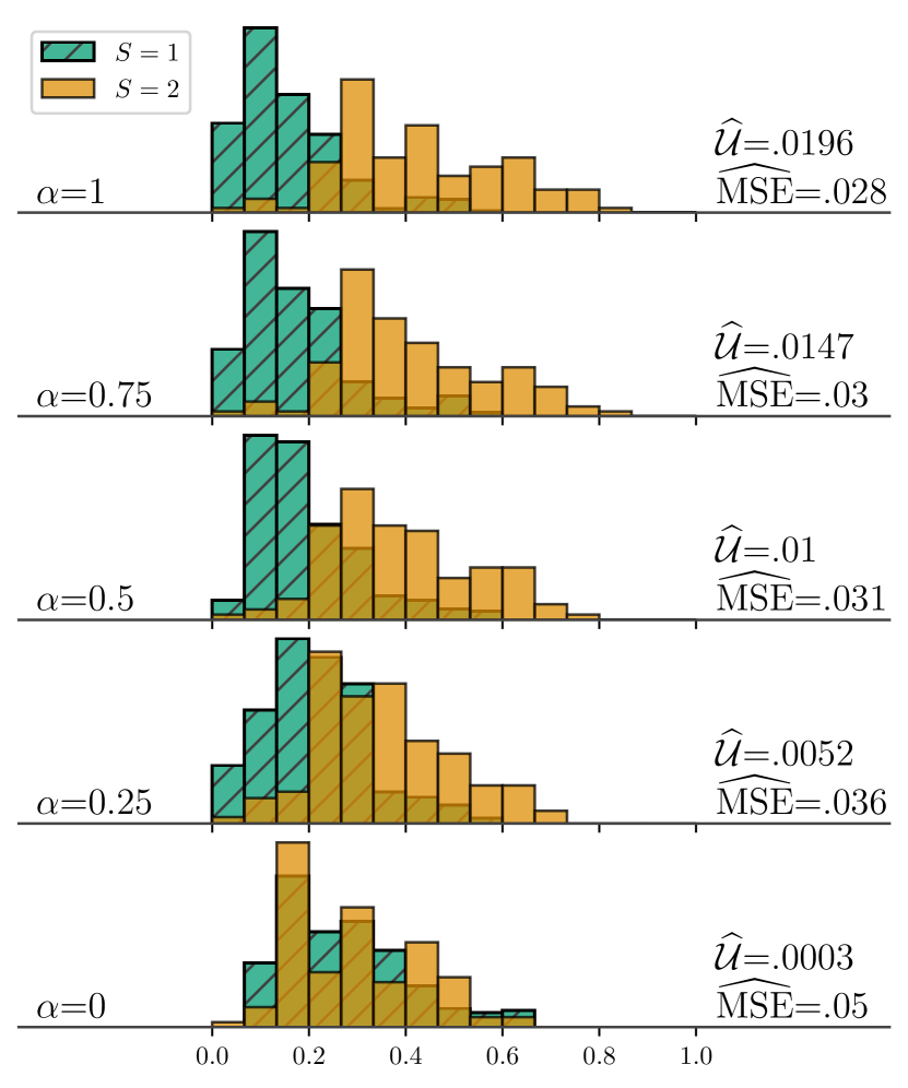
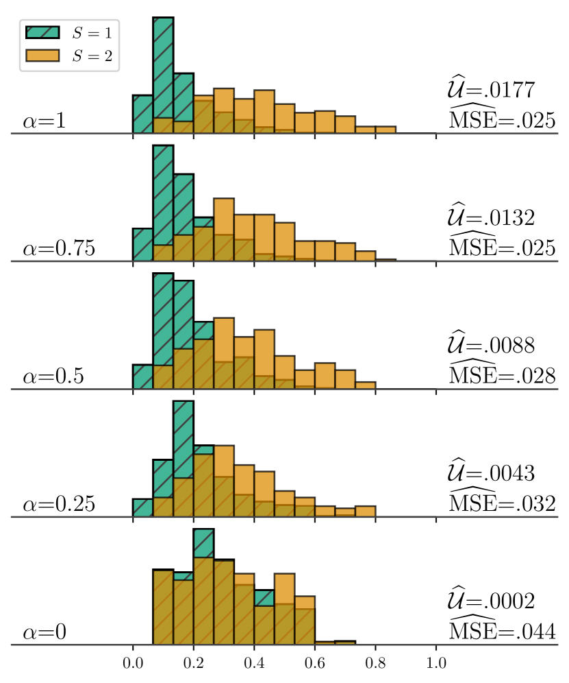
Refer to caption
(a) Evaluated on 𝒟testsubscript𝒟test\mathcal{D}_{\operatorname{test}}.
Refer to caption
(b) Evaluated on 𝒟unlabsubscript𝒟unlab\mathcal{D}_{\operatorname*{unlab}}.
Figure 8: Evolution of the empirical distributions of the post-processing method for different choices of α[0,1]𝛼01\alpha\in[0,1] coupled with the RF as the base estimator.

8.3 Ad-hoc estimator from Section 7.1: distribution equalization

We tested our post-processing procedure with two different base methods: random forest (RF) and k𝑘k-Nearest Neighbours (kNN)101010As before, we rely on scikit-learn package (Pedregosa et al., 2011) to implement those base methods.. We fitted each method on the training set 𝒟trainsubscript𝒟train\mathcal{D}_{\operatorname{train}} using 3-fold CV procedure to optimize hyper-parameters.

First, on Figure 8, we display the evolution of the group-wise distributions computed on 𝒟testsubscript𝒟test\mathcal{D}_{\operatorname{test}} (Fig. 8(a)) and on 𝒟unlabsubscript𝒟unlab\mathcal{D}_{\operatorname*{unlab}} (Fig. 8(b)) when α𝛼\alpha varies from 111 (no fairness adjustment) to 00 (estimation of fair optimal). Due to the form of the post-processing procedure, it is expected that the post-processing estimator achieves near perfect distribution matching when evaluated on the unlabeled data. This phenomenon is displayed on Fig. 8(b). Furthermore, on 𝒟testsubscript𝒟test\mathcal{D}_{\operatorname{test}}, which was never used during the training stage, the post-processing algorithm also displays a visually (and quantitatively, as indicated by risk and unfairness measures) superior performance.

8.4 The performance frontier

We repeat the splitting of the whole dataset 𝒟𝒟\mathcal{D} into the three sets for 100100100 times and, for each α[0,1]𝛼01\alpha\in[0,1], average the resulting unfairness and MSE. Then, for each method and each α[0,1]𝛼01\alpha\in[0,1] we obtain a point in the coordinates (MSE^,𝒰^)^MSE^𝒰(\widehat{\operatorname*{MSE}},\,\widehat{\mathcal{U}}) and the resulting curves (parametrized by α𝛼\alpha) are displayed in Figure 9. We note that the estimator BLS from Section 6 performs reasonably well and even dominates the post-processing based on the kNN in the regime of moderately low values α𝛼\alpha. At the same time, the post-processing coupled with the RF as the base method uniformly dominates both kNN+post-processing and BLS—model-based method of Section 6. Furthermore, on Figure 9(b) one can clearly see the main drawback of the BLS estimator—it fails to achieve a very low level of unfairness (as a point of reference compare the largest unfairness of RF and the smallest of BLS). Such a behaviour is not surprising since the Gaussian features assumption is probably violated and thus, the best we can hope for in general situation is the group-wise mean equalization.
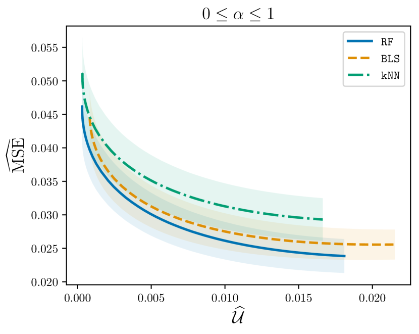
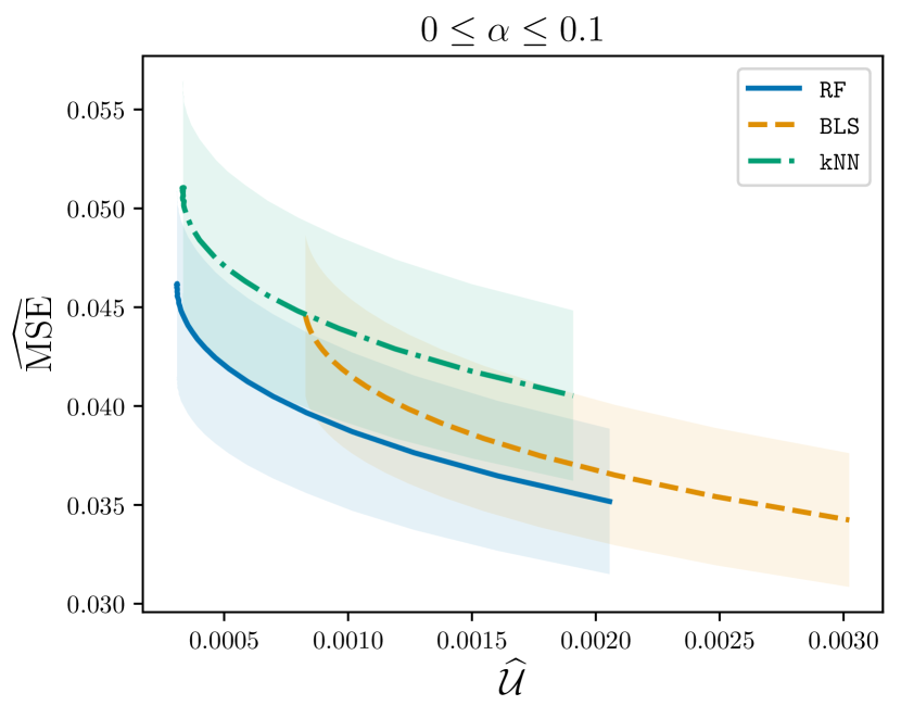
Refer to caption
(a) Performance frontier of three methods: RF+post-process; kNN+post-process; BLS from Eq. (13) for α[0,1]𝛼01\alpha\in[0,1].
Refer to caption
(b) Performance frontier of three methods: RF+post-process; kNN+post-process; BLS from Eq. (13) for α[0,0.1]𝛼00.1\alpha\in[0,0.1].
Figure 9: Performance frontiers of different families of estimators

8.5 Ad-hoc estimator from Section 7.1: verifying properties

Even though the ad-hoc procedure in Section 7.1 directly mimics the expression for the α𝛼\alpha-RI, it is actually a randomized prediction. Hence, as suggested by one of the reviewers, it is interesting to empirically verify the order-preservation and the mean stability properties announced in Section 4.

Order preservation. Note that, while the order preservation property was stated for the α𝛼\alpha-RI relevant to the Bayes optimal fsuperscript𝑓f^{*}, it should be understood relative to the base estimator for the post-processing procedure . To this end, we fit the post-processing operator Π^^Π\hat{\Pi} on 𝒟unlabsubscript𝒟unlab\mathcal{D}_{\operatorname*{unlab}} and, for three values of α𝛼\alpha, display

f(𝒙,s)vsf^α(𝒙,s)=αf(𝒙,s)+Π^(f)(𝒙,s)(𝒙,s)p×[K],formulae-sequence𝑓𝒙𝑠vssubscript^𝑓𝛼𝒙𝑠𝛼𝑓𝒙𝑠^Π𝑓𝒙𝑠𝒙𝑠superscript𝑝delimited-[]𝐾\displaystyle f(\boldsymbol{x},s)\qquad\text{vs}\qquad\hat{f}_{\alpha}(\boldsymbol{x},s)=\sqrt{\alpha}f(\boldsymbol{x},s)+\hat{\Pi}(f)(\boldsymbol{x},s)\qquad\qquad(\boldsymbol{x},s)\in\mathbb{R}^{p}\times[K]\enspace,

evaluated on (𝒙,s)𝒟test𝒙𝑠subscript𝒟test(\boldsymbol{x},s)\in\mathcal{D}_{\operatorname{test}}, where f𝑓f is a base-estimator trained on 𝒟trainsubscript𝒟train\mathcal{D}_{\operatorname{train}}. If the order preservation property holds, we expect to see a monotone curve for all α[0,1)𝛼01\alpha\in[0,1). Note that the curve for the reference value α=1𝛼1\alpha=1 corresponds to that of the identity mapping.
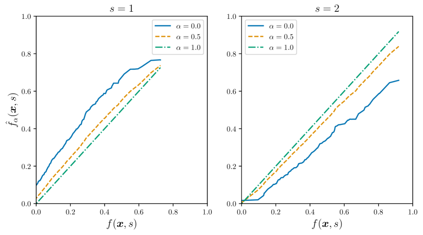
Refer to caption
Figure 10: Order preservation for the ad-hoc method
Refer to caption
Figure 11: Mean stability of the ad-hoc method

Figure 10 displays the obtained results. We observe, as expected, that the order-preservation property is approximately satisfied.

Mean stability. Concerning the mean stability, we display the following quantity

(1Ks=1K𝔼^[f^α(𝑿,S)S=s])/(1Ks=1K𝔼^[f(𝑿,S)S=s])α[0,1],1𝐾superscriptsubscript𝑠1𝐾^𝔼delimited-[]conditionalsubscript^𝑓𝛼𝑿𝑆𝑆𝑠1𝐾superscriptsubscript𝑠1𝐾^𝔼delimited-[]conditional𝑓𝑿𝑆𝑆𝑠𝛼01\displaystyle\left(\frac{1}{K}\sum_{s=1}^{K}\hat{\mathbb{E}}[\hat{f}_{\alpha}(\boldsymbol{X},S)\mid S=s]\right)\bigg{/}\left(\frac{1}{K}\sum_{s=1}^{K}\hat{\mathbb{E}}[f(\boldsymbol{X},S)\mid S=s]\right)\qquad\qquad\alpha\in[0,1]\enspace,

where 𝔼^^𝔼\hat{\mathbb{E}} is evaluated on 𝒟testsubscript𝒟test\mathcal{D}_{\operatorname{test}}. We evaluate this quantity 100100100 times to account for randomness that is present within f^αsubscript^𝑓𝛼\hat{f}_{\alpha}. Ideally, the above quantity should be equal to one for all α[0,1]𝛼01\alpha\in[0,1], which signifies that the mean stays stable along all the values of α[0,1]𝛼01\alpha\in[0,1]. We display these results on Figure 11 and observe that the mean stability property is indeed present with the standard deviation being at most 5%percent55\%.

9 Conclusion

In this work, we proposed a theoretical framework for rigorous analysis of regression problems under fairness requirements. Our framework allows to interpolate between regression under the Demographic Parity constraint and unconstrained regression, using a univariate parameter between zero and one. Within this framework we precisely quantified the risk-fairness trade-off and derived general plug-n-play lower bound. To demonstrate the generality of our results we provided minimax analysis of the linear model with systematic group-dependent bias. Finally, we have proposed a post-processing algorithm which enjoys strong theoretical guarantees and performed empirical validations both on simulated and benchmark data. For future work, it would be interesting to extend our analysis to other statistical models, providing estimators with high confidence fairness improvement.

References

  • Agarwal, Dudik and Wu (2019) {binproceedings}[author] \bauthor\bsnmAgarwal, \bfnmA.\binitsA., \bauthor\bsnmDudik, \bfnmM.\binitsM. and \bauthor\bsnmWu, \bfnmZ. S.\binitsZ. S. (\byear2019). \btitleFair Regression: Quantitative Definitions and Reduction-Based Algorithms. In \bbooktitleInternational Conference on Machine Learning. \endbibitem
  • Agarwal et al. (2018) {barticle}[author] \bauthor\bsnmAgarwal, \bfnmA.\binitsA., \bauthor\bsnmBeygelzimer, \bfnmA.\binitsA., \bauthor\bsnmDudík, \bfnmM.\binitsM., \bauthor\bsnmLangford, \bfnmJ.\binitsJ. and \bauthor\bsnmWallach, \bfnmH.\binitsH. (\byear2018). \btitleA reductions approach to fair classification. \bjournalInternational Conference on Machine Learning. \endbibitem
  • Agueh and Carlier (2011) {barticle}[author] \bauthor\bsnmAgueh, \bfnmM.\binitsM. and \bauthor\bsnmCarlier, \bfnmG.\binitsG. (\byear2011). \btitleBarycenters in the Wasserstein space. \bjournalSIAM Journal on Mathematical Analysis \bvolume43 \bpages904–924. \endbibitem
  • Audibert and Catoni (2011) {barticle}[author] \bauthor\bsnmAudibert, \bfnmJ. -Y. \binitsJ. and \bauthor\bsnmCatoni, \bfnmO.\binitsO. (\byear2011). \btitleRobust linear least squares regression. \bjournalThe Annals of Statistics \bvolume39 \bpages2766–2794. \endbibitem
  • Baharlouei et al. (2019) {barticle}[author] \bauthor\bsnmBaharlouei, \bfnmS.\binitsS., \bauthor\bsnmNouiehed, \bfnmM.\binitsM., \bauthor\bsnmBeirami, \bfnmA.\binitsA. and \bauthor\bsnmRazaviyayn, \bfnmM.\binitsM. (\byear2019). \btitleRényi Fair Inference. \bjournalarXiv preprint arXiv:1906.12005. \endbibitem
  • Barber et al. (2021) {barticle}[author] \bauthor\bsnmBarber, \bfnmR.\binitsR., \bauthor\bsnmCandes, \bfnmE.\binitsE., \bauthor\bsnmRamdas, \bfnmA.\binitsA. and \bauthor\bsnmTibshirani, \bfnmR.\binitsR. (\byear2021). \btitleThe limits of distribution-free conditional predictive inference. \bjournalInformation and Inference: A Journal of the IMA \bvolume10 \bpages455–482. \endbibitem
  • Barocas, Hardt and Narayanan (2019) {bbook}[author] \bauthor\bsnmBarocas, \bfnmSolon\binitsS., \bauthor\bsnmHardt, \bfnmMoritz\binitsM. and \bauthor\bsnmNarayanan, \bfnmArvind\binitsA. (\byear2019). \btitleFairness and Machine Learning. \bpublisherfairmlbook.org \bnotehttp://www.fairmlbook.org. \endbibitem
  • Bellec (2017) {barticle}[author] \bauthor\bsnmBellec, \bfnmP.\binitsP. (\byear2017). \btitleOptimal exponential bounds for aggregation of density estimators. \bjournalBernoulli \bvolume23 \bpages219–248. \endbibitem
  • Berk et al. (2017) {binproceedings}[author] \bauthor\bsnmBerk, \bfnmR.\binitsR., \bauthor\bsnmHeidari, \bfnmH.\binitsH., \bauthor\bsnmJabbari, \bfnmS.\binitsS., \bauthor\bsnmJoseph, \bfnmM.\binitsM., \bauthor\bsnmKearns, \bfnmM.\binitsM., \bauthor\bsnmMorgenstern, \bfnmJ.\binitsJ., \bauthor\bsnmNeel, \bfnmS.\binitsS. and \bauthor\bsnmRoth, \bfnmA.\binitsA. (\byear2017). \btitleA convex framework for fair regression. In \bbooktitleFairness, Accountability, and Transparency in Machine Learning. \endbibitem
  • Bertsimas, Farias and Trichakis (2012) {barticle}[author] \bauthor\bsnmBertsimas, \bfnmD.\binitsD., \bauthor\bsnmFarias, \bfnmV.\binitsV. and \bauthor\bsnmTrichakis, \bfnmN.\binitsN. (\byear2012). \btitleOn the efficiency-fairness trade-off. \bjournalManagement Science \bvolume58 \bpages2234–2250. \endbibitem
  • Bobkov and Ledoux (2019) {bbook}[author] \bauthor\bsnmBobkov, \bfnmS.\binitsS. and \bauthor\bsnmLedoux, \bfnmM.\binitsM. (\byear2019). \btitleOne-Dimensional Empirical Measures, Order Statistics, and Kantorovich Transport Distances. \bseriesMemoirs of the American Mathematical Society. \bpublisherAmerican Mathematical Society. \endbibitem
  • Calders, Kamiran and Pechenizkiy (2009) {binproceedings}[author] \bauthor\bsnmCalders, \bfnmT.\binitsT., \bauthor\bsnmKamiran, \bfnmF.\binitsF. and \bauthor\bsnmPechenizkiy, \bfnmM.\binitsM. (\byear2009). \btitleBuilding classifiers with independency constraints. In \bbooktitleIEEE international conference on Data mining. \endbibitem
  • Calders et al. (2013) {binproceedings}[author] \bauthor\bsnmCalders, \bfnmT.\binitsT., \bauthor\bsnmKarim, \bfnmA.\binitsA., \bauthor\bsnmKamiran, \bfnmF.\binitsF., \bauthor\bsnmAli, \bfnmW.\binitsW. and \bauthor\bsnmZhang, \bfnmX.\binitsX. (\byear2013). \btitleControlling attribute effect in linear regression. In \bbooktitleIEEE International Conference on Data Mining. \endbibitem
  • Catoni (2004) {bbook}[author] \bauthor\bsnmCatoni, \bfnmO.\binitsO. (\byear2004). \btitleStatistical learning theory and stochastic optimization. Ecole d’été de probabilités de Saint-Flour XXXI-2001. \bpublisherSpringer \bnoteCollection : Lecture notes in mathematics n°1851. \endbibitem
  • Chen, Gao and Ren (2016) {barticle}[author] \bauthor\bsnmChen, \bfnmM.\binitsM., \bauthor\bsnmGao, \bfnmC.\binitsC. and \bauthor\bsnmRen, \bfnmZ.\binitsZ. (\byear2016). \btitleA general decision theory for Huber’s ϵitalic-ϵ\epsilon-contamination model. \bjournalElectronic Journal of Statistics \bvolume10 \bpages3752–3774. \endbibitem
  • Chen, Gao and Ren (2018) {barticle}[author] \bauthor\bsnmChen, \bfnmM.\binitsM., \bauthor\bsnmGao, \bfnmC.\binitsC. and \bauthor\bsnmRen, \bfnmZ.\binitsZ. (\byear2018). \btitleRobust covariance and scatter matrix estimation under Huber’s contamination model. \bjournalThe Annals of Statistics \bvolume46 \bpages1932–1960. \endbibitem
  • Chiappa et al. (2020) {binproceedings}[author] \bauthor\bsnmChiappa, \bfnmS.\binitsS., \bauthor\bsnmJiang, \bfnmR.\binitsR., \bauthor\bsnmStepleton, \bfnmT.\binitsT., \bauthor\bsnmPacchiano, \bfnmA.\binitsA., \bauthor\bsnmJiang, \bfnmH.\binitsH. and \bauthor\bsnmAslanides, \bfnmJ.\binitsJ. (\byear2020). \btitleA general approach to fairness with optimal transport. In \bbooktitleAAAI. \endbibitem
  • Chzhen et al. (2020a) {barticle}[author] \bauthor\bsnmChzhen, \bfnmE.\binitsE., \bauthor\bsnmDenis, \bfnmC.\binitsC., \bauthor\bsnmHebiri, \bfnmM.\binitsM., \bauthor\bsnmOneto, \bfnmL.\binitsL. and \bauthor\bsnmPontil, \bfnmM.\binitsM. (\byear2020a). \btitleFair Regression with Wasserstein Barycenters. \bjournalAdvances in Neural Information Processing Systems. \endbibitem
  • Chzhen et al. (2020b) {barticle}[author] \bauthor\bsnmChzhen, \bfnmE.\binitsE., \bauthor\bsnmDenis, \bfnmC.\binitsC., \bauthor\bsnmHebiri, \bfnmM.\binitsM., \bauthor\bsnmOneto, \bfnmL.\binitsL. and \bauthor\bsnmPontil, \bfnmM.\binitsM. (\byear2020b). \btitleFair Regression via Plug-in Estimator and Recalibration With Statistical Guarantees. \bjournalAdvances in Neural Information Processing Systems. \endbibitem
  • del Barrio, Gordaliza and Loubes (2020) {barticle}[author] \bauthor\bparticledel \bsnmBarrio, \bfnmE.\binitsE., \bauthor\bsnmGordaliza, \bfnmP.\binitsP. and \bauthor\bsnmLoubes, \bfnmJ. -M. \binitsJ. (\byear2020). \btitleReview of Mathematical frameworks for Fairness in Machine Learning. \bjournalarXiv preprint arXiv:2005.13755. \endbibitem
  • Donini et al. (2018) {binproceedings}[author] \bauthor\bsnmDonini, \bfnmM.\binitsM., \bauthor\bsnmOneto, \bfnmL.\binitsL., \bauthor\bsnmBen-David, \bfnmS.\binitsS., \bauthor\bsnmShawe-Taylor, \bfnmJ. S.\binitsJ. S. and \bauthor\bsnmPontil, \bfnmM.\binitsM. (\byear2018). \btitleEmpirical risk minimization under fairness constraints. In \bbooktitleNeural Information Processing Systems. \endbibitem
  • Dwork et al. (2012) {binproceedings}[author] \bauthor\bsnmDwork, \bfnmC.\binitsC., \bauthor\bsnmHardt, \bfnmM.\binitsM., \bauthor\bsnmPitassi, \bfnmT.\binitsT., \bauthor\bsnmReingold, \bfnmO.\binitsO. and \bauthor\bsnmZemel, \bfnmR.\binitsR. (\byear2012). \btitleFairness through awareness. In \bbooktitleProceedings of the 3rd innovations in theoretical computer science conference \bpages214–226. \endbibitem
  • Fitzsimons et al. (2018) {barticle}[author] \bauthor\bsnmFitzsimons, \bfnmJ.\binitsJ., \bauthor\bsnmAli, \bfnmA. Al\binitsA. A., \bauthor\bsnmOsborne, \bfnmM.\binitsM. and \bauthor\bsnmRoberts, \bfnmS.\binitsS. (\byear2018). \btitleEquality Constrained Decision Trees: For the Algorithmic Enforcement of Group Fairness. \bjournalarXiv preprint arXiv:1810.05041. \endbibitem
  • Fitzsimons et al. (2019) {barticle}[author] \bauthor\bsnmFitzsimons, \bfnmJ.\binitsJ., \bauthor\bsnmAl Ali, \bfnmA.\binitsA., \bauthor\bsnmOsborne, \bfnmM.\binitsM. and \bauthor\bsnmRoberts, \bfnmS.\binitsS. (\byear2019). \btitleA general framework for fair regression. \bjournalEntropy \bvolume21 \bpages741. \endbibitem
  • Fréchet (1957) {barticle}[author] \bauthor\bsnmFréchet, \bfnmM.\binitsM. (\byear1957). \btitleSur la distance de deux lois de probabilité. \bjournalComtes Rendus Hebdomadaires des Seances de l’Academie des Sciences \bvolume244 \bpages689–692. \endbibitem
  • Gangbo and Święch (1998) {barticle}[author] \bauthor\bsnmGangbo, \bfnmW.\binitsW. and \bauthor\bsnmŚwięch, \bfnmA.\binitsA. (\byear1998). \btitleOptimal maps for the multidimensional Monge-Kantorovich problem. \bjournalCommunications on Pure and Applied Mathematics: A Journal Issued by the Courant Institute of Mathematical Sciences \bvolume51 \bpages23–45. \endbibitem
  • Gilbert (1952) {barticle}[author] \bauthor\bsnmGilbert, \bfnmE.\binitsE. (\byear1952). \btitleA comparison of signalling alphabets. \bjournalThe Bell system technical journal \bvolume31 \bpages504–522. \endbibitem
  • Gordaliza et al. (2019) {binproceedings}[author] \bauthor\bsnmGordaliza, \bfnmP.\binitsP., \bauthor\bsnmDel Barrio, \bfnmE.\binitsE., \bauthor\bsnmFabrice, \bfnmG.\binitsG. and \bauthor\bsnmLoubes, \bfnmJ. M.\binitsJ. M. (\byear2019). \btitleObtaining fairness using optimal transport theory. In \bbooktitleInternational Conference on Machine Learning. \endbibitem
  • Györfi et al. (2006) {bbook}[author] \bauthor\bsnmGyörfi, \bfnmL.\binitsL., \bauthor\bsnmKohler, \bfnmM.\binitsM., \bauthor\bsnmKrzyzak, \bfnmA.\binitsA. and \bauthor\bsnmWalk, \bfnmH.\binitsH. (\byear2006). \btitleA distribution-free theory of nonparametric regression. \bpublisherSpringer Science & Business Media. \endbibitem
  • Haas (2019) {barticle}[author] \bauthor\bsnmHaas, \bfnmC.\binitsC. (\byear2019). \btitleThe Price of Fairness-A Framework to Explore Trade-Offs in Algorithmic Fairness. \bjournalarXiv preprint arXiv. \endbibitem
  • Hardt, Price and Srebro (2016) {binproceedings}[author] \bauthor\bsnmHardt, \bfnmM.\binitsM., \bauthor\bsnmPrice, \bfnmE.\binitsE. and \bauthor\bsnmSrebro, \bfnmN.\binitsN. (\byear2016). \btitleEquality of opportunity in supervised learning. In \bbooktitleNeural Information Processing Systems. \endbibitem
  • Hsu, Kakade and Zhang (2012) {binproceedings}[author] \bauthor\bsnmHsu, \bfnmD.\binitsD., \bauthor\bsnmKakade, \bfnmS.\binitsS. and \bauthor\bsnmZhang, \bfnmT.\binitsT. (\byear2012). \btitleRandom design analysis of ridge regression. In \bbooktitleConference on learning theory \bpages9–1. \endbibitem
  • Hunter (2007) {barticle}[author] \bauthor\bsnmHunter, \bfnmJ. D.\binitsJ. D. (\byear2007). \btitleMatplotlib: A 2D graphics environment. \bjournalComputing in Science & Engineering \bvolume9 \bpages90–95. \endbibitem
  • Jiang et al. (2020) {barticle}[author] \bauthor\bsnmJiang, \bfnmR.\binitsR., \bauthor\bsnmPacchiano, \bfnmA.\binitsA., \bauthor\bsnmStepleton, \bfnmT.\binitsT., \bauthor\bsnmJiang, \bfnmH.\binitsH. and \bauthor\bsnmChiappa, \bfnmS.\binitsS. (\byear2020). \btitleWasserstein fair classification. \bjournalUncertainty in Artificial Intelligence Conference. \endbibitem
  • Kerkyacharian et al. (2014) {barticle}[author] \bauthor\bsnmKerkyacharian, \bfnmG.\binitsG., \bauthor\bsnmTsybakov, \bfnmA.\binitsA., \bauthor\bsnmTemlyakov, \bfnmV.\binitsV., \bauthor\bsnmPicard, \bfnmD.\binitsD. and \bauthor\bsnmKoltchinskii, \bfnmV.\binitsV. (\byear2014). \btitleOptimal exponential bounds on the accuracy of classification. \bjournalConstructive Approximation \bvolume39 \bpages421–444. \endbibitem
  • Kloeckner (2010) {barticle}[author] \bauthor\bsnmKloeckner, \bfnmB.\binitsB. (\byear2010). \btitleA geometric study of Wasserstein spaces: Euclidean spaces. \bjournalAnnali della Scuola Normale Superiore di Pisa-Classe di Scienze \bvolume9 \bpages297–323. \endbibitem
  • Komiyama and Shimao (2017) {barticle}[author] \bauthor\bsnmKomiyama, \bfnmJ.\binitsJ. and \bauthor\bsnmShimao, \bfnmH.\binitsH. (\byear2017). \btitleTwo-stage Algorithm for Fairness-aware Machine Learning. \bjournalarXiv preprint arXiv:1710.04924. \endbibitem
  • Komiyama et al. (2018) {binproceedings}[author] \bauthor\bsnmKomiyama, \bfnmJ.\binitsJ., \bauthor\bsnmTakeda, \bfnmA.\binitsA., \bauthor\bsnmHonda, \bfnmJ.\binitsJ. and \bauthor\bsnmShimao, \bfnmH.\binitsH. (\byear2018). \btitleNonconvex Optimization for Regression with Fairness Constraints. In \bbooktitleInternational Conference on Machine Learning. \endbibitem
  • Köeppen, Yoshida and Ohnishi (2014) {binproceedings}[author] \bauthor\bsnmKöeppen, \bfnmM.\binitsM., \bauthor\bsnmYoshida, \bfnmK.\binitsK. and \bauthor\bsnmOhnishi, \bfnmK.\binitsK. (\byear2014). \btitleEvolving Fair Linear Regression for the Representation of Human-Drawn Regression Lines. In \bbooktitle2014 International Conference on Intelligent Networking and Collaborative Systems \bpages296-303. \endbibitem
  • Laurent and Massart (2000) {barticle}[author] \bauthor\bsnmLaurent, \bfnmB.\binitsB. and \bauthor\bsnmMassart, \bfnmP.\binitsP. (\byear2000). \btitleAdaptive estimation of a quadratic functional by model selection. \bjournalAnnals of Statistics \bpages1302–1338. \endbibitem
  • Le Gouic and Loubes (2017) {barticle}[author] \bauthor\bsnmLe Gouic, \bfnmT.\binitsT. and \bauthor\bsnmLoubes, \bfnmJ. -M. \binitsJ. (\byear2017). \btitleExistence and consistency of Wasserstein barycenters. \bjournalProbability Theory and Related Fields \bvolume168 \bpages901–917. \endbibitem
  • Le Gouic, Loubes and Rigollet (2020) {barticle}[author] \bauthor\bsnmLe Gouic, \bfnmT.\binitsT., \bauthor\bsnmLoubes, \bfnmJ. -M. \binitsJ. and \bauthor\bsnmRigollet, \bfnmP.\binitsP. (\byear2020). \btitleProjection to Fairness in Statistical Learning. \bjournalarXiv preprint arXiv:2005.11720. \endbibitem
  • Lei and Wasserman (2014) {barticle}[author] \bauthor\bsnmLei, \bfnmJ.\binitsJ. and \bauthor\bsnmWasserman, \bfnmL.\binitsL. (\byear2014). \btitleDistribution-free prediction bands for non-parametric regression. \bjournalJournal of the Royal Statistical Society: Series B: Statistical Methodology \bpages71–96. \endbibitem
  • Lei et al. (2018) {barticle}[author] \bauthor\bsnmLei, \bfnmJ.\binitsJ., \bauthor\bsnmG’Sell, \bfnmM.\binitsM., \bauthor\bsnmRinaldo, \bfnmA.\binitsA., \bauthor\bsnmTibshirani, \bfnmR.\binitsR. and \bauthor\bsnmWasserman, \bfnmL.\binitsL. (\byear2018). \btitleDistribution-free predictive inference for regression. \bjournalJournal of the American Statistical Association \bvolume113 \bpages1094–1111. \endbibitem
  • Lipton, Chouldechova and McAuley (2018) {binproceedings}[author] \bauthor\bsnmLipton, \bfnmZ.\binitsZ., \bauthor\bsnmChouldechova, \bfnmA.\binitsA. and \bauthor\bsnmMcAuley, \bfnmJ.\binitsJ. (\byear2018). \btitleDoes mitigating ML’s impact disparity require treatment disparity? In \bbooktitleAdvances in Neural Information Processing Systems \bpages8136–8146. \endbibitem
  • Madras et al. (2018) {binproceedings}[author] \bauthor\bsnmMadras, \bfnmD.\binitsD., \bauthor\bsnmCreager, \bfnmE.\binitsE., \bauthor\bsnmPitassi, \bfnmT.\binitsT. and \bauthor\bsnmZemel, \bfnmR.\binitsR. (\byear2018). \btitleLearning Adversarially Fair and Transferable Representations. In \bbooktitleInternational Conference on Machine Learning \bpages3384–3393. \endbibitem
  • Mary, Calauzènes and El Karoui (2019) {binproceedings}[author] \bauthor\bsnmMary, \bfnmJ.\binitsJ., \bauthor\bsnmCalauzènes, \bfnmC.\binitsC. and \bauthor\bsnmEl Karoui, \bfnmN.\binitsN. (\byear2019). \btitleFairness-aware learning for continuous attributes and treatments. In \bbooktitleInternational Conference on Machine Learning \bpages4382–4391. \endbibitem
  • Mehrabi et al. (2019) {barticle}[author] \bauthor\bsnmMehrabi, \bfnmN.\binitsN., \bauthor\bsnmMorstatter, \bfnmF.\binitsF., \bauthor\bsnmSaxena, \bfnmN.\binitsN., \bauthor\bsnmLerman, \bfnmK.\binitsK. and \bauthor\bsnmGalstyan, \bfnmA.\binitsA. (\byear2019). \btitleA survey on bias and fairness in machine learning. \bjournalarXiv preprint arXiv:1908.09635. \endbibitem
  • Mourtada (2019) {barticle}[author] \bauthor\bsnmMourtada, \bfnmJ.\binitsJ. (\byear2019). \btitleExact minimax risk for linear least squares, and the lower tail of sample covariance matrices. \bjournalarXiv preprint arXiv:1912.10754. \endbibitem
  • Nemirovski (2000) {barticle}[author] \bauthor\bsnmNemirovski, \bfnmA.\binitsA. (\byear2000). \btitleTOPICS IN NON-PARAMETRIC STATISTICS. \bjournalLecture Notes in Mathematics \bvolume1738 \bpages86–282. \endbibitem
  • Olfat et al. (2020) {barticle}[author] \bauthor\bsnmOlfat, \bfnmM.\binitsM., \bauthor\bsnmSloan, \bfnmS.\binitsS., \bauthor\bsnmHespanhol, \bfnmP.\binitsP., \bauthor\bsnmPorter, \bfnmW.\binitsW., \bauthor\bsnmVasudevan, \bfnmR.\binitsR. and \bauthor\bsnmAswani, \bfnmA.\binitsA. (\byear2020). \btitleCovariance-Robust Dynamic Watermarking. \bjournalarXiv preprint arXiv:2003.13908. \endbibitem
  • Oneto and Chiappa (2020) {bincollection}[author] \bauthor\bsnmOneto, \bfnmL.\binitsL. and \bauthor\bsnmChiappa, \bfnmS.\binitsS. (\byear2020). \btitleFairness in Machine Learning. In \bbooktitleRecent Trends in Learning From Data \bpages155–196. \bpublisherSpringer. \endbibitem
  • Oneto, Donini and Pontil (2020) {binproceedings}[author] \bauthor\bsnmOneto, \bfnmLuca\binitsL., \bauthor\bsnmDonini, \bfnmMichele\binitsM. and \bauthor\bsnmPontil, \bfnmMassimiliano\binitsM. (\byear2020). \btitleGeneral fair empirical risk minimization. In \bbooktitle2020 International Joint Conference on Neural Networks (IJCNN) \bpages1–8. \bpublisherIEEE. \endbibitem
  • Oneto et al. (2020) {binproceedings}[author] \bauthor\bsnmOneto, \bfnmL.\binitsL., \bauthor\bsnmDonini, \bfnmM.\binitsM., \bauthor\bsnmPontil, \bfnmM.\binitsM. and \bauthor\bsnmMaurer, \bfnmA.\binitsA. (\byear2020). \btitleLearning Fair and Transferable Representations with Theoretical Guarantees. In \bbooktitle2020 IEEE 7th International Conference on Data Science and Advanced Analytics (DSAA) \bpages30–39. \bpublisherIEEE. \endbibitem
  • Osborne and Rubinstein (1994) {btechreport}[author] \bauthor\bsnmOsborne, \bfnmM.\binitsM. and \bauthor\bsnmRubinstein, \bfnmA.\binitsA. (\byear1994). \btitleA Course in Game Theory \btypeTechnical Report, \bpublisherThe MIT Press. \endbibitem
  • Pedregosa et al. (2011) {barticle}[author] \bauthor\bsnmPedregosa, \bfnmF.\binitsF., \bauthor\bsnmVaroquaux, \bfnmG.\binitsG., \bauthor\bsnmGramfort, \bfnmA.\binitsA., \bauthor\bsnmMichel, \bfnmV.\binitsV., \bauthor\bsnmThirion, \bfnmB.\binitsB., \bauthor\bsnmGrisel, \bfnmO.\binitsO., \bauthor\bsnmBlondel, \bfnmM.\binitsM., \bauthor\bsnmPrettenhofer, \bfnmP.\binitsP., \bauthor\bsnmWeiss, \bfnmR.\binitsR., \bauthor\bsnmDubourg, \bfnmV.\binitsV., \bauthor\bsnmVanderplas, \bfnmJ.\binitsJ., \bauthor\bsnmPassos, \bfnmA.\binitsA., \bauthor\bsnmCournapeau, \bfnmD.\binitsD., \bauthor\bsnmBrucher, \bfnmM.\binitsM., \bauthor\bsnmPerrot, \bfnmM.\binitsM. and \bauthor\bsnmDuchesnay, \bfnmE.\binitsE. (\byear2011). \btitleScikit-learn: Machine Learning in Python. \bjournalJournal of Machine Learning Research \bvolume12 \bpages2825–2830. \endbibitem
  • Pérez-Suay et al. (2017) {binproceedings}[author] \bauthor\bsnmPérez-Suay, \bfnmA.\binitsA., \bauthor\bsnmLaparra, \bfnmV.\binitsV., \bauthor\bsnmMateo-García, \bfnmG.\binitsG., \bauthor\bsnmMuñoz-Marí, \bfnmJ.\binitsJ., \bauthor\bsnmGómez-Chova, \bfnmL.\binitsL. and \bauthor\bsnmCamps-Valls, \bfnmG.\binitsG. (\byear2017). \btitleFair kernel learning. In \bbooktitleJoint European Conference on Machine Learning and Knowledge Discovery in Databases. \endbibitem
  • Plečko and Meinshausen (2020) {barticle}[author] \bauthor\bsnmPlečko, \bfnmD.\binitsD. and \bauthor\bsnmMeinshausen, \bfnmN.\binitsN. (\byear2020). \btitleFair data adaptation with quantile preservation. \bjournalJournal of Machine Learning Research \bvolume21 \bpages1–44. \endbibitem
  • Quadrianto and Sharmanska (2017) {binproceedings}[author] \bauthor\bsnmQuadrianto, \bfnmN.\binitsN. and \bauthor\bsnmSharmanska, \bfnmV.\binitsV. (\byear2017). \btitleRecycling privileged learning and distribution matching for fairness. In \bbooktitleAdvances in Neural Information Processing Systems \bpages677–688. \endbibitem
  • Raff, Sylvester and Mills (2018) {binproceedings}[author] \bauthor\bsnmRaff, \bfnmE.\binitsE., \bauthor\bsnmSylvester, \bfnmJ.\binitsJ. and \bauthor\bsnmMills, \bfnmS.\binitsS. (\byear2018). \btitleFair forests: Regularized tree induction to minimize model bias. In \bbooktitleAAAI/ACM Conference on AI, Ethics, and Society. \endbibitem
  • Rigollet and Hütter (2015) {barticle}[author] \bauthor\bsnmRigollet, \bfnmP.\binitsP. and \bauthor\bsnmHütter, \bfnmJ. -C. \binitsJ. (\byear2015). \btitleHigh dimensional statistics. \bjournalLecture notes for course 18S997. \endbibitem
  • Santambrogio (2015) {barticle}[author] \bauthor\bsnmSantambrogio, \bfnmF.\binitsF. (\byear2015). \btitleOptimal transport for applied mathematicians. \endbibitem
  • Steinberg, Reid and O’Callaghan (2020) {barticle}[author] \bauthor\bsnmSteinberg, \bfnmD.\binitsD., \bauthor\bsnmReid, \bfnmA.\binitsA. and \bauthor\bsnmO’Callaghan, \bfnmS.\binitsS. (\byear2020). \btitleFairness Measures for Regression via Probabilistic Classification. \bjournalarXiv preprint arXiv:2001.06089. \endbibitem
  • Steinberg et al. (2020) {barticle}[author] \bauthor\bsnmSteinberg, \bfnmD.\binitsD., \bauthor\bsnmReid, \bfnmA.\binitsA., \bauthor\bsnmO’Callaghan, \bfnmS.\binitsS., \bauthor\bsnmLattimore, \bfnmF.\binitsF., \bauthor\bsnmMcCalman, \bfnmL.\binitsL. and \bauthor\bsnmCaetano, \bfnmT.\binitsT. (\byear2020). \btitleFast Fair Regression via Efficient Approximations of Mutual Information. \bjournalarXiv preprint arXiv:2002.06200. \endbibitem
  • Stone (1977) {barticle}[author] \bauthor\bsnmStone, \bfnmC.\binitsC. (\byear1977). \btitleConsistent nonparametric regression. \bjournalAnn. Statist. \bpages595–620. \endbibitem
  • Tsybakov (2003) {bincollection}[author] \bauthor\bsnmTsybakov, \bfnmA.\binitsA. (\byear2003). \btitleOptimal rates of aggregation. In \bbooktitleLearning theory and kernel machines \bpages303–313. \bpublisherSpringer. \endbibitem
  • Tsybakov (2009) {bbook}[author] \bauthor\bsnmTsybakov, \bfnmA.\binitsA. (\byear2009). \btitleIntroduction to nonparametric estimation. \bseriesSpringer Series in Statistics. \bpublisherSpringer, \baddressNew York. \endbibitem
  • Van der Vaart (2000) {bbook}[author] \bauthor\bparticleVan der \bsnmVaart, \bfnmAad W\binitsA. W. (\byear2000). \btitleAsymptotic statistics \bvolume3. \bpublisherCambridge university press. \endbibitem
  • Van Der Walt, Colbert and Varoquaux (2011) {barticle}[author] \bauthor\bsnmVan Der Walt, \bfnmS.\binitsS., \bauthor\bsnmColbert, \bfnmC.\binitsC. and \bauthor\bsnmVaroquaux, \bfnmG.\binitsG. (\byear2011). \btitleThe NumPy array: a structure for efficient numerical computation. \bjournalComputing in Science & Engineering \bvolume13 \bpages22. \endbibitem
  • Varshamov (1957) {barticle}[author] \bauthor\bsnmVarshamov, \bfnmR.\binitsR. (\byear1957). \btitleEstimate of the number of signals in error correcting codes. \bjournalDokl. Akad. Nauk SSSR \bvolume117 \bpages739–-741. \endbibitem
  • Vershynin (2010) {barticle}[author] \bauthor\bsnmVershynin, \bfnmR.\binitsR. (\byear2010). \btitleIntroduction to the non-asymptotic analysis of random matrices. \bjournalarXiv preprint arXiv:1011.3027. \endbibitem
  • Villani (2003) {bbook}[author] \bauthor\bsnmVillani, \bfnmC.\binitsC. (\byear2003). \btitleTopics in Optimal Transportation. \bpublisherAmerican Mathematical Society. \endbibitem
  • Vovk, Gammerman and Shafer (2005) {bbook}[author] \bauthor\bsnmVovk, \bfnmV.\binitsV., \bauthor\bsnmGammerman, \bfnmA.\binitsA. and \bauthor\bsnmShafer, \bfnmG.\binitsG. (\byear2005). \btitleAlgorithmic learning in a random world. \bpublisherSpringer Science & Business Media. \endbibitem
  • Wick, Panda and Tristan (2019) {bincollection}[author] \bauthor\bsnmWick, \bfnmM.\binitsM., \bauthor\bsnmPanda, \bfnmS.\binitsS. and \bauthor\bsnmTristan, \bfnmJ. -B. \binitsJ. (\byear2019). \btitleUnlocking Fairness: a Trade-off Revisited. In \bbooktitleAdvances in Neural Information Processing Systems 32 \bpages8783–8792. \bpublisherCurran Associates, Inc. \endbibitem
  • Zafar et al. (2017) {binproceedings}[author] \bauthor\bsnmZafar, \bfnmM. B.\binitsM. B., \bauthor\bsnmValera, \bfnmI.\binitsI., \bauthor\bsnmGomez Rodriguez, \bfnmM.\binitsM. and \bauthor\bsnmGummadi, \bfnmK. P.\binitsK. P. (\byear2017). \btitleFairness beyond disparate treatment & disparate impact: Learning classification without disparate mistreatment. In \bbooktitleInternational Conference on World Wide Web. \endbibitem
  • Zink and Rose (2019) {barticle}[author] \bauthor\bsnmZink, \bfnmA.\binitsA. and \bauthor\bsnmRose, \bfnmS.\binitsS. (\byear2019). \btitleFair regression for health care spending. \bjournalBiometrics \bvolumen/a. \endbibitem
  • Zliobaite (2015) {barticle}[author] \bauthor\bsnmZliobaite, \bfnmI.\binitsI. (\byear2015). \btitleOn the relation between accuracy and fairness in binary classification. \bjournalarXiv preprint arXiv:1505.05723. \endbibitem

CONTENTS

\startcontents

[appendices] \printcontents[appendices]l1

Appendix A Reminder

A.1 The Wasserstein-2 distance

Additional notation. For any s[K]𝑠delimited-[]𝐾s\in[K], we denote by μ𝑿|ssubscript𝜇conditional𝑿𝑠\mu_{\boldsymbol{X}|s} the conditional distribution of the feature vector 𝑿𝑿\boldsymbol{X} knowing the attribute s𝑠s. For a probability measure μ𝜇\mu on psuperscript𝑝\mathbb{R}^{p} and a measurable function g:p:𝑔superscript𝑝g:\mathbb{R}^{p}\to\mathbb{R}, we denote by g#μ𝑔#𝜇g\#\mu the push-forward (image) measure. That is for all measurable set 𝒞𝒞\mathcal{C}\subset\mathbb{R} it holds that (g#μ)(𝒞):=μ{𝒙p:g(𝒙)𝒞}assign𝑔#𝜇𝒞𝜇conditional-set𝒙superscript𝑝𝑔𝒙𝒞(g\#\mu)(\mathcal{C})\vcentcolon=\mu\{\boldsymbol{x}\in\mathbb{R}^{p}\,:\,g(\boldsymbol{x})\in\mathcal{C}\}.

We recall basic results on the Wasserstein-2 distance on the real line. We recall that the Wasserstein-2 distance between probability distributions μ𝜇\mu and ν𝜈\nu in 𝒫2(d)subscript𝒫2superscript𝑑\mathcal{P}_{2}(\mathbb{R}^{d}), the space of measures on dsuperscript𝑑\mathbb{R}^{d} with finite second moment, is defined as

𝖶22(μ,ν)infπΓ(μ,ν){d×d𝒙𝒚22dπ(𝒙,𝒚)},superscriptsubscript𝖶22𝜇𝜈subscriptinfimum𝜋Γ𝜇𝜈subscriptsuperscript𝑑superscript𝑑superscriptsubscriptdelimited-∥∥𝒙𝒚22differential-d𝜋𝒙𝒚\displaystyle\mathsf{W}_{2}^{2}(\mu,\nu)\coloneqq\inf_{\pi\in\Gamma(\mu,\nu)}\left\{\int_{\mathbb{R}^{d}\times\mathbb{R}^{d}}\lVert\boldsymbol{x}-\boldsymbol{y}\rVert_{2}^{2}\,\mathrm{d}\pi(\boldsymbol{x},\boldsymbol{y})\right\}\enspace, (15)

where Γ(μ,ν)Γ𝜇𝜈\Gamma(\mu,\nu) denotes the collection of measures on d×dsuperscript𝑑superscript𝑑\mathbb{R}^{d}\times\mathbb{R}^{d} with marginals μ𝜇\mu and ν𝜈\nu. See (Santambrogio, 2015, Villani, 2003) for more details about Wasserstein distances and optimal transport.

The following lemma gives a closed form expression for the Wasserstein-2 distance between two univariate Gaussian distributions.

Lemma A.1 (Fréchet (1957)).

For any m0,m1,σ0,σ10formulae-sequencesubscript𝑚0subscript𝑚1subscript𝜎0subscript𝜎10m_{0},m_{1}\in\mathbb{R},\sigma_{0},\sigma_{1}\geq 0 it holds that

𝖶22(𝒩(m0,σ02),𝒩(m1,σ12))=(m0m1)2+(σ0σ1)2.superscriptsubscript𝖶22𝒩subscript𝑚0superscriptsubscript𝜎02𝒩subscript𝑚1superscriptsubscript𝜎12superscriptsubscript𝑚0subscript𝑚12superscriptsubscript𝜎0subscript𝜎12\displaystyle\mathsf{W}_{2}^{2}\Big{(}{\mathcal{N}(m_{0},\sigma_{0}^{2}),\,\mathcal{N}(m_{1},\sigma_{1}^{2})\Big{)}}=(m_{0}-m_{1})^{2}+(\sigma_{0}-\sigma_{1})^{2}\enspace.

The next lemma gives a closed form expression for the barycenter of K𝐾K univariate Gaussian distributions. It shows in particular that such barycenter is also a univariate Gaussian distribution.

Lemma A.2 (Agueh and Carlier (2011)).

Let 𝐰K𝐰superscript𝐾\boldsymbol{w}\in\mathbb{R}^{K} be a probability vector, then the solution of

minν𝒫2()s=1Kws𝖶22(𝒩(ms,σs2),ν),subscript𝜈subscript𝒫2superscriptsubscript𝑠1𝐾subscript𝑤𝑠superscriptsubscript𝖶22𝒩subscript𝑚𝑠superscriptsubscript𝜎𝑠2𝜈\displaystyle\min_{\nu\in\mathcal{P}_{2}(\mathbb{R})}\sum_{s=1}^{K}w_{s}\mathsf{W}_{2}^{2}\left(\mathcal{N}(m_{s},\sigma_{s}^{2}),\nu\right)\enspace,

is given by 𝒩(m¯,σ¯2)𝒩¯𝑚superscript¯𝜎2\mathcal{N}(\bar{m},\bar{\sigma}^{2}) with

m¯=s=1Kwsmsandσ¯=s=1Kwsσs.formulae-sequence¯𝑚superscriptsubscript𝑠1𝐾subscript𝑤𝑠subscript𝑚𝑠and¯𝜎superscriptsubscript𝑠1𝐾subscript𝑤𝑠subscript𝜎𝑠\displaystyle\bar{m}=\sum_{s=1}^{K}w_{s}m_{s}\quad\text{and}\quad\bar{\sigma}=\sum_{s=1}^{K}w_{s}\sigma_{s}\enspace.

Finally we state a lemma giving an explicit form for the transport map to the barycenter of probability distributions supported on the real line and the corresponding constant speed geodesics. See (Agueh and Carlier, 2011, Section 6.1).

Lemma A.3.

Let a1,,aKsubscript𝑎1subscript𝑎𝐾a_{1},\dots,a_{K} be non-atomic probability measures on the real line that have finite second moments, and let w1,,wKsubscript𝑤1subscript𝑤𝐾w_{1},\dots,w_{K} be positive reals that sum to 1. Denote by a¯¯𝑎\bar{a} a barycenter of those measures (w.r.t. to the Wasserstein-2 distance). For any s[K]𝑠delimited-[]𝐾s\in[K], the transport map from assubscript𝑎𝑠a_{s} to the barycenter a¯¯𝑎\bar{a} is given by

Tasa¯=(s=1KwsFs1Fs),subscript𝑇subscript𝑎𝑠¯𝑎superscriptsubscriptsuperscript𝑠1𝐾subscript𝑤superscript𝑠superscriptsubscript𝐹superscript𝑠1subscript𝐹𝑠\displaystyle T_{a_{s}\rightarrow\bar{a}}=\left(\sum_{s^{\prime}=1}^{K}w_{s^{\prime}}F_{s^{\prime}}^{-1}\circ F_{s}\right)\enspace,

where Fssubscript𝐹𝑠F_{s} is the cumulative distribution function of assubscript𝑎𝑠a_{s} and Fs1superscriptsubscript𝐹𝑠1F_{s}^{-1} denotes the generalized inverse of Fssubscript𝐹𝑠F_{s} defined as

Fs1(t)=inf{x:Fs(x)t}.superscriptsubscript𝐹𝑠1𝑡infimumconditional-set𝑥subscript𝐹𝑠𝑥𝑡\displaystyle F_{s}^{-1}(t)=\inf\{x:F_{s}(x)\geq t\}\enspace.

In particular, the constant speed geodesic γs()subscript𝛾𝑠\gamma_{s}(\cdot) from assubscript𝑎𝑠a_{s} to a¯¯𝑎\bar{a} is given by

γs(t)=((1t)Id+tTasa¯)#as,t[0,1].formulae-sequencesubscript𝛾𝑠𝑡1𝑡Id𝑡subscript𝑇subscript𝑎𝑠¯𝑎#subscript𝑎𝑠𝑡01\displaystyle\gamma_{s}(t)=((1-t)\operatorname*{Id}+tT_{a_{s}\rightarrow\bar{a}})\#a_{s},\quad t\in[0,1]\enspace.

A.2 Tail inequalities

The next result can be found in (Laurent and Massart, 2000, Lemma 1).

Lemma A.4.

Let ζ1,,ζpsubscript𝜁1subscript𝜁𝑝\zeta_{1},\ldots,\zeta_{p} be i.i.d. standard Gaussian random variables. Let 𝐚=(a1,,ap)𝐚superscriptsubscript𝑎1subscript𝑎𝑝top\boldsymbol{a}=(a_{1},\ldots,a_{p})^{\top} be component-wise non-negative, then

𝐏(j=1paj(ζj21)2𝒂2t+2𝒂t)exp(t),t0.formulae-sequence𝐏superscriptsubscript𝑗1𝑝subscript𝑎𝑗superscriptsubscript𝜁𝑗212subscriptdelimited-∥∥𝒂2𝑡2subscriptdelimited-∥∥𝒂𝑡𝑡for-all𝑡0\displaystyle\mathbf{P}\left(\sum_{j=1}^{p}a_{j}(\zeta_{j}^{2}-1)\geq 2\left\lVert\boldsymbol{a}\right\rVert_{2}\sqrt{t}+2\left\lVert\boldsymbol{a}\right\rVert_{\infty}t\right)\leq\exp(-t),\quad\forall t\geq 0\enspace.

In particular, setting 𝜻=(ζ1,,ζp)𝜻superscriptsubscript𝜁1subscript𝜁𝑝top\boldsymbol{\zeta}=(\zeta_{1},\ldots,\zeta_{p})^{\top} and applying the previous result with a1==ap=1subscript𝑎1subscript𝑎𝑝1a_{1}=\ldots=a_{p}=1 we get

𝐏(𝜻22p+2pt+2t)exp(t),t0formulae-sequence𝐏superscriptsubscriptnorm𝜻22𝑝2𝑝𝑡2𝑡𝑡for-all𝑡0\displaystyle\mathbf{P}\left(\|\boldsymbol{\zeta}\|_{2}^{2}\geq p+2\sqrt{pt}+2t\right)\leq\exp(-t),\quad\forall t\geq 0

We need one result from random matrix theory to control the smallest and largest singular values of a Gaussian matrix, see (Vershynin, 2010, Corollary 5.35).

Lemma A.5.

Let 𝐀𝐀\mathbf{A} be an N×m𝑁𝑚N\times m matrix whose entries are independent standard normal random variables. Then,

𝐏(σmin(𝐀)Nmt)𝐏(σmax(𝐀)N+m+t)exp(t2/2),t0.formulae-sequence𝐏subscript𝜎𝐀𝑁𝑚𝑡𝐏subscript𝜎𝐀𝑁𝑚𝑡superscript𝑡22for-all𝑡0\displaystyle\mathbf{P}\left(\sigma_{\min}(\mathbf{A})\leq\sqrt{N}-\sqrt{m}-t\right)\vee\mathbf{P}\left(\sigma_{\max}(\mathbf{A})\geq\sqrt{N}+\sqrt{m}+t\right)\leq\exp(-t^{2}/2),\quad\forall t\geq 0\enspace.

Appendix B Proofs for Section 4

B.1 Auxiliary results

The next result is taken from (Le Gouic, Loubes and Rigollet, 2020, Theorem 3).

Lemma B.1.

Let f:p×[K]:𝑓superscript𝑝delimited-[]𝐾f:\mathbb{R}^{p}\times[K]\to\mathbb{R} be any measurable function. Let Assumption 2.1 be satisfied, then

(f)s=1Kws𝖶22(f(,s)#μ𝑿|s,f(,s)#μ𝑿|s).𝑓superscriptsubscript𝑠1𝐾subscript𝑤𝑠superscriptsubscript𝖶22𝑓𝑠#subscript𝜇conditional𝑿𝑠superscript𝑓𝑠#subscript𝜇conditional𝑿𝑠\displaystyle\mathcal{R}(f)\geq\sum_{s=1}^{K}w_{s}\mathsf{W}_{2}^{2}\bigg{(}f(\cdot,s)\#\mu_{\boldsymbol{X}|s},f^{*}(\cdot,s)\#\mu_{\boldsymbol{X}|s}\bigg{)}\enspace.
Lemma B.2 (Minkowski’s inequality).

Let (𝒳,d)𝒳𝑑(\mathcal{X},d) be a metric space. Fix integers K2𝐾2K\geq 2, q[1,+)𝑞1q\in[1,+\infty), a weight vector 𝐰ΔK1𝐰superscriptΔ𝐾1\boldsymbol{w}\in\Delta^{K-1} and define the mapping d𝐰,q:𝒳K×𝒳K:subscript𝑑𝐰𝑞superscript𝒳𝐾superscript𝒳𝐾d_{\boldsymbol{w},q}:\mathcal{X}^{K}\times\mathcal{X}^{K}\to\mathbb{R} as

d𝒘,q(𝒂,𝒃)={s=1Kwsdq(as,bs)}1/q,for any 𝒂,𝒃𝒳K.subscript𝑑𝒘𝑞𝒂𝒃superscriptsuperscriptsubscript𝑠1𝐾subscript𝑤𝑠superscript𝑑𝑞subscript𝑎𝑠subscript𝑏𝑠1𝑞for any 𝒂,𝒃𝒳K\displaystyle d_{\boldsymbol{w},q}(\boldsymbol{a},\boldsymbol{b})=\left\{\sum_{s=1}^{K}w_{s}d^{q}(a_{s},b_{s})\right\}^{\nicefrac{{1}}{{q}}},\qquad\text{for any $\boldsymbol{a},\boldsymbol{b}\in\mathcal{X}^{K}$}\enspace.

Then, d𝐰,qsubscript𝑑𝐰𝑞d_{\boldsymbol{w},q} is a pseudo-metric on the product space 𝒳Ksuperscript𝒳𝐾\mathcal{X}^{K}.

Proof.

The mapping d𝒘,qsubscript𝑑𝒘𝑞d_{\boldsymbol{w},q} is clearly symmetric and non-negative. We only have to check the triangle inequality. Fix arbitrary 𝒂,𝒃,𝒄𝒳K𝒂𝒃𝒄superscript𝒳𝐾\boldsymbol{a},\boldsymbol{b},\boldsymbol{c}\in\mathcal{X}^{K}. Then, by triangular inequalities on the distance d𝑑d and Hölder’s inequality,

s=1Kwsdq(as,bs)superscriptsubscript𝑠1𝐾subscript𝑤𝑠superscript𝑑𝑞subscript𝑎𝑠subscript𝑏𝑠\displaystyle\sum_{s=1}^{K}w_{s}d^{q}(a_{s},b_{s}) s=1Kwsd(as,cs)dq1(as,bs)+s=1Kwsd(cs,bs)dq1(as,bs)absentsuperscriptsubscript𝑠1𝐾subscript𝑤𝑠𝑑subscript𝑎𝑠subscript𝑐𝑠superscript𝑑𝑞1subscript𝑎𝑠subscript𝑏𝑠superscriptsubscript𝑠1𝐾subscript𝑤𝑠𝑑subscript𝑐𝑠subscript𝑏𝑠superscript𝑑𝑞1subscript𝑎𝑠subscript𝑏𝑠\displaystyle\leq\sum_{s=1}^{K}w_{s}d(a_{s},c_{s})d^{q-1}(a_{s},b_{s})+\sum_{s=1}^{K}w_{s}d(c_{s},b_{s})d^{q-1}(a_{s},b_{s})
({s=1Kwsdq(as,cs)}1/q+{s=1Kwsdq(cs,bs)}1/q){s=1Kwsdq(as,bs)}11q.absentsuperscriptsuperscriptsubscript𝑠1𝐾subscript𝑤𝑠superscript𝑑𝑞subscript𝑎𝑠subscript𝑐𝑠1𝑞superscriptsuperscriptsubscript𝑠1𝐾subscript𝑤𝑠superscript𝑑𝑞subscript𝑐𝑠subscript𝑏𝑠1𝑞superscriptsuperscriptsubscript𝑠1𝐾subscript𝑤𝑠superscript𝑑𝑞subscript𝑎𝑠subscript𝑏𝑠11𝑞\displaystyle\leq\left(\left\{\sum_{s=1}^{K}w_{s}d^{q}(a_{s},c_{s})\right\}^{\nicefrac{{1}}{{q}}}+\left\{\sum_{s=1}^{K}w_{s}d^{q}(c_{s},b_{s})\right\}^{\nicefrac{{1}}{{q}}}\right)\left\{\sum_{s=1}^{K}w_{s}d^{q}(a_{s},b_{s})\right\}^{1-\frac{1}{q}}\enspace.

That is, after rearranging we obtain

d𝒘,q(𝒂,𝒃)={s=1Kwsdq(as,bs)}1/qsubscript𝑑𝒘𝑞𝒂𝒃superscriptsuperscriptsubscript𝑠1𝐾subscript𝑤𝑠superscript𝑑𝑞subscript𝑎𝑠subscript𝑏𝑠1𝑞\displaystyle d_{\boldsymbol{w},q}(\boldsymbol{a},\boldsymbol{b})=\left\{\sum_{s=1}^{K}w_{s}d^{q}(a_{s},b_{s})\right\}^{\nicefrac{{1}}{{q}}} {s=1Kwsdq(as,cs)}1/q+{s=1Kwsdq(cs,bs)}1/qabsentsuperscriptsuperscriptsubscript𝑠1𝐾subscript𝑤𝑠superscript𝑑𝑞subscript𝑎𝑠subscript𝑐𝑠1𝑞superscriptsuperscriptsubscript𝑠1𝐾subscript𝑤𝑠superscript𝑑𝑞subscript𝑐𝑠subscript𝑏𝑠1𝑞\displaystyle\leq\left\{\sum_{s=1}^{K}w_{s}d^{q}(a_{s},c_{s})\right\}^{\nicefrac{{1}}{{q}}}+\left\{\sum_{s=1}^{K}w_{s}d^{q}(c_{s},b_{s})\right\}^{\nicefrac{{1}}{{q}}}
=d𝒘,q(𝒂,𝒄)+d𝒘,q(𝒄,𝒃).absentsubscript𝑑𝒘𝑞𝒂𝒄subscript𝑑𝒘𝑞𝒄𝒃\displaystyle=d_{\boldsymbol{w},q}(\boldsymbol{a},\boldsymbol{c})+d_{\boldsymbol{w},q}(\boldsymbol{c},\boldsymbol{b})\enspace.

Lemma B.3.

Fix some q[1,+)𝑞1q\in[1,+\infty). Let 𝐚=(a1,,aK)𝒳K𝐚subscript𝑎1subscript𝑎𝐾superscript𝒳𝐾\boldsymbol{a}=(a_{1},\ldots,a_{K})\in\mathcal{X}^{K}, 𝐰=(w1,,wK)ΔK1𝐰superscriptsubscript𝑤1subscript𝑤𝐾topsuperscriptΔ𝐾1\boldsymbol{w}=(w_{1},\ldots,w_{K})^{\top}\in\Delta^{K-1}. Assume that 𝐛=(b1,,bK)𝒳K𝐛subscript𝑏1subscript𝑏𝐾superscript𝒳𝐾\boldsymbol{b}=(b_{1},\cdots,b_{K})\in\mathcal{X}^{K} satisfies (P1subscript𝑃1P_{1})–(P2subscript𝑃2P_{2}), then

{s=1Kwsdq(bs,C𝒃)}1/q={s=1Kwsdq(bs,C𝒂)}1/q.superscriptsuperscriptsubscript𝑠1𝐾subscript𝑤𝑠superscript𝑑𝑞subscript𝑏𝑠subscript𝐶𝒃1𝑞superscriptsuperscriptsubscript𝑠1𝐾subscript𝑤𝑠superscript𝑑𝑞subscript𝑏𝑠subscript𝐶𝒂1𝑞\displaystyle\left\{\sum_{s=1}^{K}w_{s}d^{q}(b_{s},C_{\boldsymbol{b}})\right\}^{\nicefrac{{1}}{{q}}}=\left\{\sum_{s=1}^{K}w_{s}d^{q}(b_{s},C_{\boldsymbol{a}})\right\}^{\nicefrac{{1}}{{q}}}\enspace.
Proof.

Let C𝒃subscript𝐶𝒃C_{\boldsymbol{b}} be a barycenter of (bs)s[K]subscriptsubscript𝑏𝑠𝑠delimited-[]𝐾(b_{s})_{s\in[K]} with weights (ws)s[K]subscriptsubscript𝑤𝑠𝑠delimited-[]𝐾(w_{s})_{s\in[K]}, then by Lemma B.2 it holds that

{s=1Kwsdq(as,C𝒃)}1/qsuperscriptsuperscriptsubscript𝑠1𝐾subscript𝑤𝑠superscript𝑑𝑞subscript𝑎𝑠subscript𝐶𝒃1𝑞\displaystyle\left\{\sum_{s=1}^{K}w_{s}d^{q}(a_{s},C_{\boldsymbol{b}})\right\}^{\nicefrac{{1}}{{q}}} {s=1Kwsdq(as,bs)}1/q+{s=1Kwsdq(bs,C𝒃)}1/q.absentsuperscriptsuperscriptsubscript𝑠1𝐾subscript𝑤𝑠superscript𝑑𝑞subscript𝑎𝑠subscript𝑏𝑠1𝑞superscriptsuperscriptsubscript𝑠1𝐾subscript𝑤𝑠superscript𝑑𝑞subscript𝑏𝑠subscript𝐶𝒃1𝑞\displaystyle\leq\left\{\sum_{s=1}^{K}w_{s}d^{q}(a_{s},b_{s})\right\}^{\nicefrac{{1}}{{q}}}+\left\{\sum_{s=1}^{K}w_{s}d^{q}(b_{s},C_{\boldsymbol{b}})\right\}^{\nicefrac{{1}}{{q}}}\enspace. (16)

The following chain of inequalities holds thanks to Eq. (16) and properties (P1subscript𝑃1P_{1})–(P2subscript𝑃2P_{2})

{s=1Kwsdq(bs,C𝒃)}1/qsuperscriptsuperscriptsubscript𝑠1𝐾subscript𝑤𝑠superscript𝑑𝑞subscript𝑏𝑠subscript𝐶𝒃1𝑞\displaystyle\left\{\sum_{s=1}^{K}w_{s}d^{q}(b_{s},C_{\boldsymbol{b}})\right\}^{\nicefrac{{1}}{{q}}} {s=1Kwsdq(as,C𝒃)}1/q{s=1Kwsdq(as,bs)}1/qabsentsuperscriptsuperscriptsubscript𝑠1𝐾subscript𝑤𝑠superscript𝑑𝑞subscript𝑎𝑠subscript𝐶𝒃1𝑞superscriptsuperscriptsubscript𝑠1𝐾subscript𝑤𝑠superscript𝑑𝑞subscript𝑎𝑠subscript𝑏𝑠1𝑞\displaystyle\geq\left\{\sum_{s=1}^{K}w_{s}d^{q}(a_{s},C_{\boldsymbol{b}})\right\}^{\nicefrac{{1}}{{q}}}-\left\{\sum_{s=1}^{K}w_{s}d^{q}(a_{s},b_{s})\right\}^{\nicefrac{{1}}{{q}}}
{s=1Kwsdq(as,C𝒂)}1/q{s=1Kwsdq(as,bs)}1/qabsentsuperscriptsuperscriptsubscript𝑠1𝐾subscript𝑤𝑠superscript𝑑𝑞subscript𝑎𝑠subscript𝐶𝒂1𝑞superscriptsuperscriptsubscript𝑠1𝐾subscript𝑤𝑠superscript𝑑𝑞subscript𝑎𝑠subscript𝑏𝑠1𝑞\displaystyle\geq\left\{\sum_{s=1}^{K}w_{s}d^{q}(a_{s},C_{\boldsymbol{a}})\right\}^{\nicefrac{{1}}{{q}}}-\left\{\sum_{s=1}^{K}w_{s}d^{q}(a_{s},b_{s})\right\}^{\nicefrac{{1}}{{q}}}
=1α1/q{s=1Kwsdq(bs,C𝒂)}1/q1α1/qα1/q{s=1Kwsdq(bs,C𝒂)}1/qabsent1superscript𝛼1𝑞superscriptsuperscriptsubscript𝑠1𝐾subscript𝑤𝑠superscript𝑑𝑞subscript𝑏𝑠subscript𝐶𝒂1𝑞1superscript𝛼1𝑞superscript𝛼1𝑞superscriptsuperscriptsubscript𝑠1𝐾subscript𝑤𝑠superscript𝑑𝑞subscript𝑏𝑠subscript𝐶𝒂1𝑞\displaystyle=\frac{1}{{\alpha}^{\nicefrac{{1}}{{q}}}}\left\{\sum_{s=1}^{K}w_{s}d^{q}(b_{s},C_{\boldsymbol{a}})\right\}^{\nicefrac{{1}}{{q}}}-\frac{1{-}{\alpha}^{\nicefrac{{1}}{{q}}}}{{\alpha}^{\nicefrac{{1}}{{q}}}}\left\{\sum_{s=1}^{K}w_{s}d^{q}(b_{s},C_{\boldsymbol{a}})\right\}^{\nicefrac{{1}}{{q}}}
={s=1Kwsdq(bs,C𝒂)}1/q.absentsuperscriptsuperscriptsubscript𝑠1𝐾subscript𝑤𝑠superscript𝑑𝑞subscript𝑏𝑠subscript𝐶𝒂1𝑞\displaystyle=\left\{\sum_{s=1}^{K}w_{s}d^{q}(b_{s},C_{\boldsymbol{a}})\right\}^{\nicefrac{{1}}{{q}}}\enspace.

The converse inequality follows from the definition of C𝒃subscript𝐶𝒃C_{\boldsymbol{b}}, which concludes the proof. ∎

B.2 Proof of Proposition 4.1

Let α[0,1]𝛼01\alpha\in[0,1]. For any s[K]𝑠delimited-[]𝐾s\in[K], define

assubscript𝑎𝑠\displaystyle a_{s} =f(,s)#μ𝑿|s=νs,absentsuperscript𝑓𝑠#subscript𝜇conditional𝑿𝑠superscriptsubscript𝜈𝑠\displaystyle=f^{*}(\cdot,s)\#\mu_{\boldsymbol{X}|s}=\nu_{s}^{*}\enspace, (17)

Let γssubscript𝛾𝑠\gamma_{s} be the (constant-speed) geodesic between assubscript𝑎𝑠a_{s} and C𝒂subscript𝐶𝒂C_{\boldsymbol{a}} i.e., γs(0)=assubscript𝛾𝑠0subscript𝑎𝑠\gamma_{s}(0)=a_{s}, γs(1)=C𝒂subscript𝛾𝑠1subscript𝐶𝒂\gamma_{s}(1)=C_{\boldsymbol{a}} and 𝖶2(γs(t1),γs(t2))=|t2t1|𝖶2(as,C𝒂)subscript𝖶2subscript𝛾𝑠subscript𝑡1subscript𝛾𝑠subscript𝑡2subscript𝑡2subscript𝑡1subscript𝖶2subscript𝑎𝑠subscript𝐶𝒂\mathsf{W}_{2}(\gamma_{s}(t_{1}),\gamma_{s}(t_{2}))=|t_{2}-t_{1}|\mathsf{W}_{2}(a_{s},C_{\boldsymbol{a}}) for any t1,t2[0,1]subscript𝑡1subscript𝑡201t_{1},t_{2}\in[0,1]. Note that the uniqueness of the geodesic come from the particular structure of the Wasserstein-2 space on the real line, see e.g., (Kloeckner, 2010, Section 2.2). We define bs:=γs(1α)assignsubscript𝑏𝑠subscript𝛾𝑠1𝛼b_{s}\vcentcolon=\gamma_{s}(1{-}\sqrt{\alpha}) for s[K]𝑠delimited-[]𝐾s\in[K]. Let us show that 𝒃=(bs)s[K]𝒃subscriptsubscript𝑏𝑠𝑠delimited-[]𝐾\boldsymbol{b}=(b_{s})_{s\in[K]} satisfies the properties (P1subscript𝑃1P_{1})–(P2subscript𝑃2P_{2}) of the Geometric Lemma 4.3 when considering 𝒂=(as)s[K]𝒂subscriptsubscript𝑎𝑠𝑠delimited-[]𝐾\boldsymbol{a}=(a_{s})_{s\in[K]} with the weights (ws)s[K]subscriptsubscript𝑤𝑠𝑠delimited-[]𝐾(w_{s})_{s\in[K]} and d𝖶2𝑑subscript𝖶2d\equiv\mathsf{W}_{2}. By construction of bs=γs(1α)subscript𝑏𝑠subscript𝛾𝑠1𝛼b_{s}=\gamma_{s}(1{-}\sqrt{\alpha}), we have

𝖶2(bs,C𝒂)=α𝖶2(as,C𝒂),subscript𝖶2subscript𝑏𝑠subscript𝐶𝒂𝛼subscript𝖶2subscript𝑎𝑠subscript𝐶𝒂\displaystyle\mathsf{W}_{2}(b_{s},C_{\boldsymbol{a}})=\sqrt{\alpha}\mathsf{W}_{2}(a_{s},C_{\boldsymbol{a}})\enspace, (18)
𝖶2(bs,as)=(1α)𝖶2(as,C𝒂).subscript𝖶2subscript𝑏𝑠subscript𝑎𝑠1𝛼subscript𝖶2subscript𝑎𝑠subscript𝐶𝒂\displaystyle\mathsf{W}_{2}(b_{s},a_{s})=(1{-}\sqrt{\alpha})\mathsf{W}_{2}(a_{s},C_{\boldsymbol{a}})\enspace. (19)

This shows that 𝒃=(bs)s[K]𝒃subscriptsubscript𝑏𝑠𝑠delimited-[]𝐾\boldsymbol{b}=(b_{s})_{s\in[K]} satisfies (P1subscript𝑃1P_{1}) and (P2subscript𝑃2P_{2}). Therefore, using Lemma 4.3 we get

s=1Kws𝖶22(bs,as)=inf𝒃𝒫2K(){s=1Kws𝖶22(bs,as):s=1KwsW22(bs,C𝒃)αs=1Kwsd2(as,C𝒂)}.superscriptsubscript𝑠1𝐾subscript𝑤𝑠superscriptsubscript𝖶22subscript𝑏𝑠subscript𝑎𝑠subscriptinfimum𝒃subscriptsuperscript𝒫𝐾2conditional-setsuperscriptsubscript𝑠1𝐾subscript𝑤𝑠superscriptsubscript𝖶22subscript𝑏𝑠subscript𝑎𝑠superscriptsubscript𝑠1𝐾subscript𝑤𝑠subscriptsuperscript𝑊22subscript𝑏𝑠subscript𝐶𝒃𝛼superscriptsubscript𝑠1𝐾subscript𝑤𝑠superscript𝑑2subscript𝑎𝑠subscript𝐶𝒂\displaystyle\sum_{s=1}^{K}w_{s}\mathsf{W}_{2}^{2}(b_{s},a_{s})=\inf_{\boldsymbol{b}\in\mathcal{P}^{K}_{2}(\mathbb{R})}\left\{\sum_{s=1}^{K}w_{s}\mathsf{W}_{2}^{2}(b_{s},a_{s})\,:\,\sum_{s=1}^{K}w_{s}W^{2}_{2}(b_{s},C_{\boldsymbol{b}}){\leq}{\alpha}\sum_{s=1}^{K}w_{s}d^{2}(a_{s},C_{\boldsymbol{a}})\right\}\enspace. (20)

Finally, thanks to the Assumption 2.1 which says that that as=νssubscript𝑎𝑠superscriptsubscript𝜈𝑠a_{s}=\nu_{s}^{*} is atomless the constant speed geodesic γssubscript𝛾𝑠\gamma_{s} between assubscript𝑎𝑠a_{s} and C𝒂subscript𝐶𝒂C_{\boldsymbol{a}} can be written as

γs(t)subscript𝛾𝑠𝑡\displaystyle\gamma_{s}(t) =((1t)Id+t(s=1KwsFas1Fas))#asabsent1𝑡Id𝑡superscriptsubscriptsuperscript𝑠1𝐾subscript𝑤superscript𝑠superscriptsubscript𝐹subscript𝑎superscript𝑠1subscript𝐹subscript𝑎𝑠#subscript𝑎𝑠\displaystyle=\left((1-t)\operatorname*{Id}+t\left(\sum_{s^{\prime}=1}^{K}w_{s^{\prime}}F_{a_{s^{\prime}}}^{-1}\circ F_{a_{s}}\right)\right)\#a_{s}
={((1t)Id+t(s=1KwsFas1Fas))f(,s)}#μ𝑿|s,t[0,1].formulae-sequenceabsent1𝑡Id𝑡superscriptsubscriptsuperscript𝑠1𝐾subscript𝑤superscript𝑠superscriptsubscript𝐹subscript𝑎superscript𝑠1subscript𝐹subscript𝑎𝑠superscript𝑓𝑠#subscript𝜇conditional𝑿𝑠𝑡01\displaystyle=\left\{\left((1-t)\operatorname*{Id}+t\left(\sum_{s^{\prime}=1}^{K}w_{s^{\prime}}F_{a_{s^{\prime}}}^{-1}\circ F_{a_{s}}\right)\right)\circ f^{*}(\cdot,s)\right\}\#\mu_{\boldsymbol{X}|s},\quad t\in[0,1]\enspace.

See Appendix A.1 for details about the first equality. Substituting t=1α𝑡1𝛼t=1{-}\sqrt{\alpha} to γssubscript𝛾𝑠\gamma_{s}, the expression for bssubscript𝑏𝑠b_{s} is

bs={(αId+(1α)(s=1KwsFas1Fas))f(,s)}#μ𝑿|s.subscript𝑏𝑠𝛼Id1𝛼superscriptsubscriptsuperscript𝑠1𝐾subscript𝑤superscript𝑠superscriptsubscript𝐹subscript𝑎superscript𝑠1subscript𝐹subscript𝑎𝑠superscript𝑓𝑠#subscript𝜇conditional𝑿𝑠\displaystyle b_{s}=\left\{\left(\sqrt{\alpha}\operatorname*{Id}+\big{(}1{-}\sqrt{\alpha}\big{)}\left(\sum_{s^{\prime}=1}^{K}w_{s^{\prime}}F_{a_{s^{\prime}}}^{-1}\circ F_{a_{s}}\right)\right)\circ f^{*}(\cdot,s)\right\}\#\mu_{\boldsymbol{X}|s}\enspace. (21)

We define fαsuperscriptsubscript𝑓𝛼f_{\alpha}^{*} for all (𝒙,s)p×[K]𝒙𝑠superscript𝑝delimited-[]𝐾(\boldsymbol{x},s)\in\mathbb{R}^{p}\times[K] as

fα(𝒙,s)=αf(𝒙,s)+(1α)s=1KwsFas1(Fas(f(𝒙,s))),superscriptsubscript𝑓𝛼𝒙𝑠𝛼superscript𝑓𝒙𝑠1𝛼superscriptsubscriptsuperscript𝑠1𝐾subscript𝑤superscript𝑠superscriptsubscript𝐹subscript𝑎superscript𝑠1subscript𝐹subscript𝑎𝑠superscript𝑓𝒙𝑠\displaystyle f_{\alpha}^{*}(\boldsymbol{x},s)=\sqrt{\alpha}f^{*}(\boldsymbol{x},s)+(1{-}\sqrt{\alpha})\sum_{s^{\prime}=1}^{K}w_{s^{\prime}}F_{a_{s^{\prime}}}^{-1}\left(F_{a_{s}}(f^{*}(\boldsymbol{x},s)\right))\enspace, (22)

then after Eq. (21) it holds that bs=fα(,s)#μ𝑿|ssubscript𝑏𝑠subscriptsuperscript𝑓𝛼𝑠#subscript𝜇conditional𝑿𝑠b_{s}=f^{*}_{\alpha}(\cdot,s)\#\mu_{\boldsymbol{X}|s} and

𝖶22(bs,as)=𝔼[(f(𝑿,S)fα(𝑿,S))2S=s].superscriptsubscript𝖶22subscript𝑏𝑠subscript𝑎𝑠𝔼delimited-[]conditionalsuperscriptsuperscript𝑓𝑿𝑆subscriptsuperscript𝑓𝛼𝑿𝑆2𝑆𝑠\displaystyle\mathsf{W}_{2}^{2}(b_{s},a_{s})=\mathbb{E}\left[(f^{*}(\boldsymbol{X},S)-f^{*}_{\alpha}(\boldsymbol{X},S))^{2}\mid S=s\right]\enspace. (23)

with 𝒰(fα)=α𝒰(f)𝒰subscriptsuperscript𝑓𝛼𝛼𝒰superscript𝑓\mathcal{U}(f^{*}_{\alpha})=\alpha\,\mathcal{U}(f^{*}). Moreover, Lemma B.1 implies that for any f𝑓f such that 𝒰(f)α𝒰(f)𝒰𝑓𝛼𝒰superscript𝑓\mathcal{U}(f)\leq\alpha\,\mathcal{U}(f^{*}) we have

𝔼(f(X,S)f(X,S))2s=1Kws𝖶22(bs,as)𝔼superscriptsuperscript𝑓𝑋𝑆𝑓𝑋𝑆2superscriptsubscript𝑠1𝐾subscript𝑤𝑠superscriptsubscript𝖶22subscript𝑏𝑠subscript𝑎𝑠\displaystyle\mathbb{E}(f^{*}(X,S)-f(X,S))^{2}\geq\sum_{s=1}^{K}w_{s}\mathsf{W}_{2}^{2}(b_{s},a_{s}) =s=1Kws𝔼[(f(𝑿,S)fα(𝑿,S))2S=s]absentsuperscriptsubscript𝑠1𝐾subscript𝑤𝑠𝔼delimited-[]conditionalsuperscriptsuperscript𝑓𝑿𝑆subscriptsuperscript𝑓𝛼𝑿𝑆2𝑆𝑠\displaystyle=\sum_{s=1}^{K}w_{s}\mathbb{E}\left[(f^{*}(\boldsymbol{X},S)-f^{*}_{\alpha}(\boldsymbol{X},S))^{2}\mid S=s\right]
=(fα).absentsubscriptsuperscript𝑓𝛼\displaystyle=\mathcal{R}(f^{*}_{\alpha})\enspace.

Thus, fαsubscriptsuperscript𝑓𝛼f^{*}_{\alpha} is the optimal fair prediction with α𝛼\alpha relative improvement. The proof is concluded.

B.3 Proof of Proposition 4.7

Proof.

For λ=0𝜆0\lambda=0, the statement trivially holds. Fix some λ(0,+)𝜆0\lambda\in(0,+\infty). Following the Pareto frontier interpretation, the minimum of the functional (f)+λ𝒰(f)𝑓𝜆𝒰𝑓\mathcal{R}(f)+\lambda\cdot\mathcal{U}(f) equals to some F0superscript𝐹0F^{*}\geq 0 if and only if, in the coordinates (,𝒰)𝒰(\mathcal{R},\mathcal{U}), the line {(,𝒰)2:+λ𝒰=F}conditional-set𝒰superscript2𝜆𝒰superscript𝐹\left\{(\mathcal{R},\mathcal{U})\in\mathbb{R}^{2}\,:\,\mathcal{R}+\lambda\cdot\mathcal{U}=F^{*}\right\} is tangent to the Pareto frontier curve {((1α)2,α)𝒰(f)}α[0,1]subscriptsuperscript1𝛼2𝛼𝒰superscript𝑓𝛼01\big{\{}((1{-}\sqrt{\alpha})^{2},\,\alpha)\cdot\mathcal{U}(f^{*})\big{\}}_{\alpha\in[0,1]}. Thus, writing this condition explicitly, it should hold that

λ=1𝒰(f)𝒰(f,λ).𝜆1𝒰superscript𝑓𝒰superscript𝑓𝜆\displaystyle-\lambda=1-\sqrt{\frac{\mathcal{U}(f^{*})}{\mathcal{U}(f^{*,\lambda})}}\enspace.

Hence, at the minimum f,λsuperscript𝑓𝜆f^{*,\lambda} of (f)+λ𝒰(f)𝑓𝜆𝒰𝑓\mathcal{R}(f)+\lambda\cdot\mathcal{U}(f) it holds that 𝒰(f,λ)=1(1+λ)2𝒰(f)𝒰superscript𝑓𝜆1superscript1𝜆2𝒰superscript𝑓\mathcal{U}(f^{*,\lambda})=\tfrac{1}{(1+\lambda)^{2}}\cdot\mathcal{U}(f^{*}). ∎

Appendix C Proof of Theorem 5.3

To ease the notation we write δnsubscript𝛿𝑛\delta_{n} instead of δn(,Θ,t)subscript𝛿𝑛Θ𝑡\delta_{n}(\mathcal{F},\Theta,t). We also define

Ψ(f^,(f,𝜽)):=𝐏(f,𝜽)(1/2(f^)δn1/2(1α)𝒰1/2(f)).assignΨ^𝑓superscript𝑓𝜽subscript𝐏superscript𝑓𝜽superscript12^𝑓superscriptsubscript𝛿𝑛121𝛼superscript𝒰12superscript𝑓\displaystyle\Psi(\hat{f},(f^{*},\boldsymbol{\theta}))\vcentcolon=\mathbf{P}_{(f^{*},\boldsymbol{\theta})}\left(\mathcal{R}^{\nicefrac{{1}}{{2}}}(\hat{f})\geq\delta_{n}^{\nicefrac{{1}}{{2}}}\vee(1{-}\sqrt{\alpha}){\mathcal{U}^{\nicefrac{{1}}{{2}}}({f^{*}})}\right)\enspace.

We split the proof according to two complementary cases.

Case 1: there exists (f,𝜽)×Θsuperscript𝑓𝜽Θ(f^{*},\boldsymbol{\theta})\in{\mathcal{F}}\times\Theta such that δn(1α)2𝒰(f)subscript𝛿𝑛superscript1𝛼2𝒰superscript𝑓\delta_{n}\leq(1{-}\sqrt{\alpha})^{2}\mathcal{U}({f^{*}}). In this case, for such couple (f,𝜽)×Θsuperscript𝑓𝜽Θ(f^{*},\boldsymbol{\theta})\in{\mathcal{F}}\times\Theta and for any estimator f^^(α,t)^𝑓subscript^𝛼superscript𝑡\hat{f}\in\widehat{\mathcal{F}}_{(\alpha,t^{\prime})} we have Case: q(1,)𝑞1q\in(1,\infty). At first we proceed similarly:

𝐄[|FA(A)FB(B)|q]𝐄[{𝐏(|BB~||AB|+|A~B~|(A,B))}q].𝐄delimited-[]superscriptsubscript𝐹𝐴𝐴subscript𝐹𝐵𝐵𝑞𝐄delimited-[]superscript𝐏𝐵~𝐵𝐴𝐵conditional~𝐴~𝐵𝐴𝐵𝑞\displaystyle\mathbf{E}[\left\lvert F_{A}(A)-F_{B}(B)\right\rvert^{q}]\leq\mathbf{E}\left[\left\{\mathbf{P}\left(\lvert B-\tilde{B}\rvert\leq\lvert A-B\rvert+\lvert\tilde{A}-\tilde{B}\rvert\mid(A,B)\right)\right\}^{q}\right]\enspace.

Furthermore, for any δ>0𝛿0\delta>0, we can deduce by Markov’s inequality

𝐏(|BB~||AB|+|A~B~|(A,B))𝐏𝐵~𝐵𝐴𝐵conditional~𝐴~𝐵𝐴𝐵\displaystyle\mathbf{P}\left(\lvert B-\tilde{B}\rvert\leq\lvert A-B\rvert+\lvert\tilde{A}-\tilde{B}\rvert\mid(A,B)\right) 𝐏(|BB~|δB)absent𝐏𝐵~𝐵conditional𝛿𝐵\displaystyle\leq\mathbf{P}(\lvert B-\tilde{B}\rvert\leq\delta\mid B)
+𝐏(δ|AB|+|A~B~|(A,B))𝐏𝛿𝐴𝐵conditional~𝐴~𝐵𝐴𝐵\displaystyle\phantom{\leq}+\mathbf{P}\left(\delta\leq\lvert A-B\rvert+\lvert\tilde{A}-\tilde{B}\rvert\mid(A,B)\right)
2CBδ+𝔼[(|AB|+|A~B~|)q1(A,B)]δq1.absent2subscript𝐶𝐵𝛿𝔼delimited-[]conditionalsuperscript𝐴𝐵~𝐴~𝐵𝑞1𝐴𝐵superscript𝛿𝑞1\displaystyle\leq 2C_{B}\delta+\frac{\mathbb{E}[(\lvert A-B\rvert+\lvert\tilde{A}-\tilde{B}\rvert)^{q-1}\mid(A,B)]}{\delta^{q-1}}\enspace.

Minimizing the above expression over δ>0𝛿0\delta>0 we deduce that

𝐏(|BB~||AB|+|A~B~|(A,B))CB1(1/q)Cq(𝔼[(|AB|+|A~B~|)q1(A,B)])1/q,𝐏𝐵~𝐵𝐴𝐵conditional~𝐴~𝐵𝐴𝐵superscriptsubscript𝐶𝐵11𝑞superscriptsubscript𝐶𝑞superscript𝔼delimited-[]conditionalsuperscript𝐴𝐵~𝐴~𝐵𝑞1𝐴𝐵1𝑞\displaystyle\mathbf{P}\left(\lvert B-\tilde{B}\rvert\leq\lvert A-B\rvert+\lvert\tilde{A}-\tilde{B}\rvert\mid(A,B)\right)\leq C_{B}^{1-(\nicefrac{{1}}{{q}})}C_{q}^{\prime}\left(\mathbb{E}[(\lvert A-B\rvert+\lvert\tilde{A}-\tilde{B}\rvert)^{q-1}\mid(A,B)]\right)^{\nicefrac{{1}}{{q}}}\enspace,

where Cq=q((q1)/2)1/qsuperscriptsubscript𝐶𝑞𝑞superscript𝑞121𝑞C_{q}^{\prime}=q(\nicefrac{{(q-1)}}{{2}})^{\nicefrac{{1}}{{q}}} Thus, the claimed bound:

𝐄[|FA(A)FB(B)|q]𝐄delimited-[]superscriptsubscript𝐹𝐴𝐴subscript𝐹𝐵𝐵𝑞\displaystyle\mathbf{E}[\left\lvert F_{A}(A)-F_{B}(B)\right\rvert^{q}] CBq1(Cq)q𝔼[(|AB|+|A~B~|)q1]CqCBq1𝔼|AB|q1.absentsuperscriptsubscript𝐶𝐵𝑞1superscriptsuperscriptsubscript𝐶𝑞𝑞𝔼delimited-[]superscript𝐴𝐵~𝐴~𝐵𝑞1subscript𝐶𝑞superscriptsubscript𝐶𝐵𝑞1𝔼superscript𝐴𝐵𝑞1\displaystyle\leq C_{B}^{q-1}(C_{q}^{\prime})^{q}\mathbb{E}[(\lvert A-B\rvert+\lvert\tilde{A}-\tilde{B}\rvert)^{q-1}]\leq C_{q}C_{B}^{q-1}\mathbb{E}\lvert A-B\rvert^{q-1}\enspace.

Case: |AB|M𝐴𝐵𝑀|A-B|\leq M almost surely. In this case the result follows from the following chain of inequalities:

𝐄[|FA(A)FB(B)|q]𝐄delimited-[]superscriptsubscript𝐹𝐴𝐴subscript𝐹𝐵𝐵𝑞\displaystyle\mathbf{E}[\left\lvert F_{A}(A)-F_{B}(B)\right\rvert^{q}] 𝐄[{𝐏(|BB~||AB|+|A~B~|(A,B))}q]absent𝐄delimited-[]superscript𝐏𝐵~𝐵𝐴𝐵conditional~𝐴~𝐵𝐴𝐵𝑞\displaystyle\leq\mathbf{E}\left[\left\{\mathbf{P}\left(\lvert B-\tilde{B}\rvert\leq\lvert A-B\rvert+\lvert\tilde{A}-\tilde{B}\rvert\mid(A,B)\right)\right\}^{q}\right]
𝐄[{𝐏(|BB~|2M(A,B))}q]4qCBqMq.absent𝐄delimited-[]superscript𝐏𝐵~𝐵conditional2𝑀𝐴𝐵𝑞superscript4𝑞superscriptsubscript𝐶𝐵𝑞superscript𝑀𝑞\displaystyle\leq\mathbf{E}\left[\left\{\mathbf{P}\left(\lvert B-\tilde{B}\rvert\leq 2M\mid(A,B)\right)\right\}^{q}\right]\leq 4^{q}C_{B}^{q}M^{q}\enspace.

The proof is concluded. ∎

Appendix F Relation between 𝒰KSsubscript𝒰KS\mathcal{U}_{\operatorname{KS}} and 𝒰𝒰\mathcal{U}

Lemma F.1.

Let μ,ν𝜇𝜈\mu,\nu be two univariate measures such that μ𝜇\mu admits a density w.r.t. the Lebesgue measure bounded by Cμsubscript𝐶𝜇C_{\mu}, then

KS(μ,ν)2Cμ𝖶1(μ,ν).KS𝜇𝜈2subscript𝐶𝜇subscript𝖶1𝜇𝜈\displaystyle\operatorname{KS}(\mu,\nu)\leq 2\sqrt{C_{\mu}\mathsf{W}_{1}(\mu,\nu)}\enspace.
Proposition F.2.

Fix some measurable f:p×[K]:𝑓superscript𝑝delimited-[]𝐾f:\mathbb{R}^{p}\times[K]\to\mathbb{R}. Assume that as=f(,s)#μs𝒫2()subscript𝑎𝑠𝑓𝑠#subscript𝜇𝑠subscript𝒫2a_{s}=f(\cdot,s)\#\mu_{s}\in\mathcal{P}_{2}(\mathbb{R}) and it admits density bounded by Cf,ssubscript𝐶𝑓𝑠C_{f,s} for all s[K]𝑠delimited-[]𝐾s\in[K], then

𝒰KS(f)1/𝒘8C¯f𝒰1/4(f),subscript𝒰KS𝑓subscriptnorm1𝒘8subscript¯𝐶𝑓superscript𝒰14𝑓\displaystyle\mathcal{U}_{\operatorname{KS}}(f)\leq\|\nicefrac{{1}}{{\boldsymbol{w}}}\|_{\infty}\sqrt{8\bar{C}_{f}}\cdot\mathcal{U}^{1/4}(f)\enspace,

where C¯f=s=1KwsCf,ssubscript¯𝐶𝑓superscriptsubscript𝑠1𝐾subscript𝑤𝑠subscript𝐶𝑓𝑠\bar{C}_{f}=\sum_{s=1}^{K}w_{s}C_{f,s}.

Proof.

We set as=Law(f(𝑿,S)S=s)subscript𝑎𝑠Lawconditional𝑓𝑿𝑆𝑆𝑠a_{s}=\operatorname{Law}(f(\boldsymbol{X},S)\mid S{=}s) and a=s=1Kwsas𝑎superscriptsubscript𝑠1𝐾subscript𝑤𝑠subscript𝑎𝑠a=\sum_{s=1}^{K}w_{s}a_{s}. Therefore, thanks to assumption of the proposition and Lemma F.1 we can write

𝒰KS(f):=s=1KKS(as,a)1/𝒘s=1KwsKS(as,a)21/𝒘s=1KwsCf,s1/2W11/2(as,a).assignsubscript𝒰KS𝑓superscriptsubscript𝑠1𝐾KSsubscript𝑎𝑠𝑎subscriptnorm1𝒘superscriptsubscript𝑠1𝐾subscript𝑤𝑠KSsubscript𝑎𝑠𝑎2subscriptnorm1𝒘superscriptsubscript𝑠1𝐾subscript𝑤𝑠superscriptsubscript𝐶𝑓𝑠12subscriptsuperscript𝑊121subscript𝑎𝑠𝑎\displaystyle\mathcal{U}_{\operatorname{KS}}(f)\vcentcolon=\sum_{s=1}^{K}\operatorname{KS}(a_{s},a)\leq\|\nicefrac{{1}}{{\boldsymbol{w}}}\|_{\infty}\sum_{s=1}^{K}w_{s}\operatorname{KS}(a_{s},a)\leq 2\|\nicefrac{{1}}{{\boldsymbol{w}}}\|_{\infty}\sum_{s=1}^{K}w_{s}C_{f,s}^{\nicefrac{{1}}{{2}}}W^{\nicefrac{{1}}{{2}}}_{1}(a_{s},a)\enspace.

Furthermore we can write for any measure ν𝒫2()𝜈subscript𝒫2\nu\in\mathcal{P}_{2}(\mathbb{R}) that

𝒰KS(f)subscript𝒰KS𝑓\displaystyle\mathcal{U}_{\operatorname{KS}}(f) (a)21/𝒘s=1KwsCf,s1/2{s=1Kws𝖶1(as,as)}1/2superscript𝑎absent2subscriptnorm1𝒘superscriptsubscript𝑠1𝐾subscript𝑤𝑠superscriptsubscript𝐶𝑓𝑠12superscriptsuperscriptsubscriptsuperscript𝑠1𝐾subscript𝑤superscript𝑠subscript𝖶1subscript𝑎𝑠subscript𝑎superscript𝑠12\displaystyle\stackrel{{\scriptstyle(a)}}{{\leq}}2\|\nicefrac{{1}}{{\boldsymbol{w}}}\|_{\infty}\sum_{s=1}^{K}w_{s}C_{f,s}^{\nicefrac{{1}}{{2}}}\left\{\sum_{s^{\prime}=1}^{K}w_{s^{\prime}}\mathsf{W}_{1}(a_{s},a_{s^{\prime}})\right\}^{\nicefrac{{1}}{{2}}}
(b)21/𝒘s=1KwsCf,s1/2{𝖶1(as,ν)+s=1Kws𝖶1(as,ν)}1/2.superscript𝑏absent2subscriptnorm1𝒘superscriptsubscript𝑠1𝐾subscript𝑤𝑠superscriptsubscript𝐶𝑓𝑠12superscriptsubscript𝖶1subscript𝑎𝑠𝜈superscriptsubscriptsuperscript𝑠1𝐾subscript𝑤superscript𝑠subscript𝖶1subscript𝑎superscript𝑠𝜈12\displaystyle\stackrel{{\scriptstyle(b)}}{{\leq}}2\|\nicefrac{{1}}{{\boldsymbol{w}}}\|_{\infty}\sum_{s=1}^{K}w_{s}C_{f,s}^{\nicefrac{{1}}{{2}}}\left\{\mathsf{W}_{1}(a_{s},\nu)+\sum_{s^{\prime}=1}^{K}w_{s^{\prime}}\mathsf{W}_{1}(a_{s^{\prime}},\nu)\right\}^{\nicefrac{{1}}{{2}}}\enspace.

In the above inequalities (a)𝑎(a) follows from the convexity of 𝖶1(as,)subscript𝖶1subscript𝑎𝑠\mathsf{W}_{1}(a_{s},\cdot) (see e.g.,  Bobkov and Ledoux, 2019, Section 4.1) and (b)𝑏(b) uses the triangle inequality. Applying the Cauchy–Schwarz inequality we obtain

𝒰KS(f)subscript𝒰KS𝑓\displaystyle\mathcal{U}_{\operatorname{KS}}(f) 21/𝒘{s=1KwsCf,s}1/2{s=1Kws(𝖶1(as,ν)+s=1Kws𝖶1(as,ν))}1/2absent2subscriptnorm1𝒘superscriptsuperscriptsubscript𝑠1𝐾subscript𝑤𝑠subscript𝐶𝑓𝑠12superscriptsuperscriptsubscript𝑠1𝐾subscript𝑤𝑠subscript𝖶1subscript𝑎𝑠𝜈superscriptsubscriptsuperscript𝑠1𝐾subscript𝑤superscript𝑠subscript𝖶1subscript𝑎superscript𝑠𝜈12\displaystyle\leq 2\|\nicefrac{{1}}{{\boldsymbol{w}}}\|_{\infty}\left\{\sum_{s=1}^{K}w_{s}C_{f,s}\right\}^{\nicefrac{{1}}{{2}}}\left\{\sum_{s=1}^{K}w_{s}\left(\mathsf{W}_{1}(a_{s},\nu)+\sum_{s^{\prime}=1}^{K}w_{s^{\prime}}\mathsf{W}_{1}(a_{s^{\prime}},\nu)\right)\right\}^{\nicefrac{{1}}{{2}}}
=23/21/𝒘{s=1KwsCf,s}1/2{s=1Kws𝖶1(as,ν)}1/2absentsuperscript232subscriptnorm1𝒘superscriptsuperscriptsubscript𝑠1𝐾subscript𝑤𝑠subscript𝐶𝑓𝑠12superscriptsuperscriptsubscript𝑠1𝐾subscript𝑤𝑠subscript𝖶1subscript𝑎𝑠𝜈12\displaystyle=2^{\nicefrac{{3}}{{2}}}\|\nicefrac{{1}}{{\boldsymbol{w}}}\|_{\infty}\left\{\sum_{s=1}^{K}w_{s}C_{f,s}\right\}^{\nicefrac{{1}}{{2}}}\left\{\sum_{s=1}^{K}w_{s}\mathsf{W}_{1}(a_{s},\nu)\right\}^{\nicefrac{{1}}{{2}}}
(c)23/21/𝒘{s=1KwsCf,s}1/2{s=1Kws𝖶12(as,ν)}1/4,superscript𝑐absentsuperscript232subscriptnorm1𝒘superscriptsuperscriptsubscript𝑠1𝐾subscript𝑤𝑠subscript𝐶𝑓𝑠12superscriptsuperscriptsubscript𝑠1𝐾subscript𝑤𝑠superscriptsubscript𝖶12subscript𝑎𝑠𝜈14\displaystyle\stackrel{{\scriptstyle(c)}}{{\leq}}2^{\nicefrac{{3}}{{2}}}\|\nicefrac{{1}}{{\boldsymbol{w}}}\|_{\infty}\left\{\sum_{s=1}^{K}w_{s}C_{f,s}\right\}^{\nicefrac{{1}}{{2}}}\left\{\sum_{s=1}^{K}w_{s}\mathsf{W}_{1}^{2}(a_{s},\nu)\right\}^{\nicefrac{{1}}{{4}}}\enspace,

where (c)𝑐(c) uses the Cauchy–Schwarz inequality one more time. Finally, setting ν𝜈\nu as the Wasserstein-2 barycenter of a1,,aKsubscript𝑎1subscript𝑎𝐾a_{1},\ldots,a_{K} and using the fact that 𝖶1(μ,ν)𝖶2(μ,ν)subscript𝖶1𝜇𝜈subscript𝖶2𝜇𝜈\mathsf{W}_{1}(\mu,\nu)\leq\mathsf{W}_{2}(\mu,\nu) we deduce that

𝒰KS(f)23/21/𝒘{s=1KwsCf,s}1/2𝒰1/4(f).subscript𝒰KS𝑓superscript232subscriptnorm1𝒘superscriptsuperscriptsubscript𝑠1𝐾subscript𝑤𝑠subscript𝐶𝑓𝑠12superscript𝒰14𝑓\displaystyle\mathcal{U}_{\operatorname{KS}}(f)\leq 2^{\nicefrac{{3}}{{2}}}\|\nicefrac{{1}}{{\boldsymbol{w}}}\|_{\infty}\left\{\sum_{s=1}^{K}w_{s}C_{f,s}\right\}^{\nicefrac{{1}}{{2}}}\mathcal{U}^{1/4}(f)\enspace.

The proof is concluded. ∎

Appendix G Extension to qsubscript𝑞{\ell_{q}} losses

In this section we provide an extension of the derived theory for the case of qsubscript𝑞\ell_{q} losses with q[1,+)𝑞1q\in[1,+\infty). In other words, instead of the 2subscript2\ell_{2}-based risk and unfairness we define

q(f)subscript𝑞𝑓\displaystyle\mathcal{R}_{q}(f) =s=1Kws𝔼[|f(𝑿,S)f(𝑿,S)|qS=s],absentsuperscriptsubscript𝑠1𝐾subscript𝑤𝑠𝔼delimited-[]conditionalsuperscript𝑓𝑿𝑆superscript𝑓𝑿𝑆𝑞𝑆𝑠\displaystyle=\sum_{s=1}^{K}w_{s}\mathbb{E}\left[\left\lvert f(\boldsymbol{X},S)-f^{*}(\boldsymbol{X},S)\right\rvert^{q}\mid S=s\right]\enspace,
𝒰q(f)subscript𝒰𝑞𝑓\displaystyle\mathcal{U}_{q}(f) =minν𝒫q()s=1Kws𝖶qq(Law(f(𝑿,S)S=s),ν).absentsubscript𝜈subscript𝒫𝑞superscriptsubscript𝑠1𝐾subscript𝑤𝑠superscriptsubscript𝖶𝑞𝑞Lawconditional𝑓𝑿𝑆𝑆𝑠𝜈\displaystyle=\min_{\nu\in\mathcal{P}_{q}(\mathbb{R})}\sum_{s=1}^{K}w_{s}\mathsf{W}_{q}^{q}\left(\operatorname{Law}(f(\boldsymbol{X},S)\mid S=s),\,\nu\right)\enspace.

In this section we will work under the following assumption, which is a straightforward adaptation of Assumption 2.1 to handle q[1,){2}𝑞12q\in[1,\infty)\setminus\{2\}.

Assumption G.1.

The measures {νs}s[K]subscriptsubscriptsuperscript𝜈𝑠𝑠delimited-[]𝐾\{\nu^{*}_{s}\}_{s\in[K]} are non-atomic and have finite q𝑞q-moments.

Theorem G.2 (q𝑞q-Optimal and the trade-off).

Fix some q[1,)𝑞1q\in[1,\infty) and let Assumption 2.1 be satisfied. Then, for any α[0,1]𝛼01\alpha\in[0,1], a fα,qsubscriptsuperscript𝑓𝛼𝑞f^{*}_{\alpha,q} solution of

minf:p×[K]{q(f):𝒰q(f)α𝒰q(f)},subscript:𝑓superscript𝑝delimited-[]𝐾:subscript𝑞𝑓subscript𝒰𝑞𝑓𝛼subscript𝒰𝑞superscript𝑓\displaystyle\min_{f:\mathbb{R}^{p}\times[K]\to\mathbb{R}}\left\{\mathcal{R}_{q}(f)\,:\,\mathcal{U}_{q}(f)\leq\alpha\cdot\mathcal{U}_{q}(f^{*})\right\}\enspace,

can be written for all (𝐱,s)p×[K]𝐱𝑠superscript𝑝delimited-[]𝐾(\boldsymbol{x},s)\in\mathbb{R}^{p}\times[K] as

fα,q(𝒙,s)=α1/qf(𝒙,s)+(1α1/q)argminy{s=1Kws|Fνs1Fνsf(𝒙,s)y|q}.subscriptsuperscript𝑓𝛼𝑞𝒙𝑠superscript𝛼1𝑞superscript𝑓𝒙𝑠1superscript𝛼1𝑞subscriptargmin𝑦superscriptsubscriptsuperscript𝑠1𝐾subscript𝑤superscript𝑠superscriptsubscriptsuperscript𝐹1subscriptsuperscript𝜈superscript𝑠subscript𝐹subscriptsuperscript𝜈𝑠superscript𝑓𝒙𝑠𝑦𝑞\displaystyle f^{*}_{\alpha,q}(\boldsymbol{x},s)=\alpha^{\nicefrac{{1}}{{q}}}f^{*}(\boldsymbol{x},s)+\left(1{-}\alpha^{\nicefrac{{1}}{{q}}}\right)\cdot\operatorname*{arg\,min}_{y\in\mathbb{R}}\left\{\sum_{s^{\prime}=1}^{K}w_{s^{\prime}}\left\lvert F^{-1}_{\nu^{*}_{s^{\prime}}}\circ F_{\nu^{*}_{s}}\circ f^{*}(\boldsymbol{x},s)-y\right\rvert^{q}\right\}\enspace. (58)

Furthermore, it holds that

q(fα,q)=(1α1/q)q𝒰q(f)and𝒰q(fα,q)=α𝒰q(f).formulae-sequencesubscript𝑞subscriptsuperscript𝑓𝛼𝑞superscript1superscript𝛼1𝑞𝑞subscript𝒰𝑞superscript𝑓andsubscript𝒰𝑞subscriptsuperscript𝑓𝛼𝑞𝛼subscript𝒰𝑞superscript𝑓\displaystyle\mathcal{R}_{q}(f^{*}_{\alpha,q})=\left(1-\alpha^{\nicefrac{{1}}{{q}}}\right)^{q}\cdot\mathcal{U}_{q}(f^{*})\qquad\text{and}\qquad\mathcal{U}_{q}(f^{*}_{\alpha,q})=\alpha\cdot\mathcal{U}_{q}(f^{*})\enspace.
Remark G.3.

Note that this result is a strict generalization of Proposition 4.1. Furthermore, it should be noted that for q=1𝑞1q=1 the optimization problem appearing in Eq. (58) (description of fα,1subscriptsuperscript𝑓𝛼1f^{*}_{\alpha,1}) does not necessarily admit a unique minimizer (whenever K𝐾K is even). Meanwhile, for q>1𝑞1q>1 the objective function is strictly convex and the minimizer is a singleton. We also observe that all the properties except the fourth one established in Section 4 still hold for fα,qsubscriptsuperscript𝑓𝛼𝑞f^{*}_{\alpha,q}. The fourth property—mean stability—is intrinsic to the case q=2𝑞2q=2, as the minimizer appearing in Eq. (58) admit a closed form expression. Note also that the ad-hoc procedure developed in Section 7.1 for q=2𝑞2q=2 can be straightforwardly extended to any q[1,)𝑞1q\in[1,\infty).

Proof of Theorem G.2.

The proof is almost identical to that of Proposition 4.1. Thus, we only develop the modifications that need to be introduced. In particular, as for the case of q=2𝑞2q=2, our goal is to apply Lemma G.5 below (instead of Lemma 4.3). To this end, we need a way to build geodesics in (𝒫q(),𝖶q)subscript𝒫𝑞subscript𝖶𝑞(\mathcal{P}_{q}(\mathbb{R}),\mathsf{W}_{q}) and suitable expressions for q𝑞q-barycenters. The first part (geodesics) is addressed by  (Santambrogio, 2015, Theorem 5.27) (instead of (Kloeckner, 2010, Section 2.2)) and gives identical description of geodesics for all q[1,)𝑞1q\in[1,\infty). A closed form expressions for q𝑞q-barycenters (𝒫q(),𝖶q)subscript𝒫𝑞subscript𝖶𝑞(\mathcal{P}_{q}(\mathbb{R}),\mathsf{W}_{q}) is derived in Lemma G.6 (used instead of Lemma A.3) which we prove below. ∎

Definition G.4 (q𝑞q-barycenter).

Fix some q[1,)𝑞1q\in[1,\infty). We say that a metric space (𝒳,d)𝒳𝑑(\mathcal{X},d) satisfies the q𝑞q-barycenter property if for any weights 𝐰ΔK1𝐰superscriptΔ𝐾1\boldsymbol{w}\in\Delta^{K-1} and tuple 𝐚=(a1,,aK)𝒳K𝐚subscript𝑎1subscript𝑎𝐾superscript𝒳𝐾\boldsymbol{a}=(a_{1},\ldots,a_{K})\in\mathcal{X}^{K} there exists a barycenter

C𝒂𝒘argminC𝒳s=1Kwsdq(as,C).subscript𝐶subscript𝒂𝒘subscriptargmin𝐶𝒳superscriptsubscript𝑠1𝐾subscript𝑤𝑠superscript𝑑𝑞subscript𝑎𝑠𝐶\displaystyle C_{\boldsymbol{a}_{\boldsymbol{w}}}\in\operatorname*{arg\,min}_{C\in\mathcal{X}}\sum_{s=1}^{K}w_{s}d^{q}(a_{s},C)\enspace.

Moreover, for any tuple 𝐚=(a1,,aK)𝒳K𝐚subscript𝑎1subscript𝑎𝐾superscript𝒳𝐾\boldsymbol{a}=(a_{1},\ldots,a_{K})\in\mathcal{X}^{K} we denote111111When there is no ambiguity in the weights 𝐰𝐰\boldsymbol{w} we simply write C𝐚subscript𝐶𝐚C_{\boldsymbol{a}}. by C𝐚𝐰subscript𝐶subscript𝐚𝐰C_{\boldsymbol{a}_{\boldsymbol{w}}} a barycenter of 𝐚𝐚\boldsymbol{a} weighted by 𝐰ΔK1𝐰superscriptΔ𝐾1\boldsymbol{w}\in\Delta^{K-1}.

Lemma G.5 (Abstract geometric lemma).

Fix some q[1,+)𝑞1q\in[1,+\infty). Let (𝒳,d)𝒳𝑑(\mathcal{X},d) be a metric space satisfying the q𝑞q-barycenter property. Let 𝐚=(a1,,aK)𝒳K𝐚subscript𝑎1subscript𝑎𝐾superscript𝒳𝐾\boldsymbol{a}=(a_{1},\ldots,a_{K})\in\mathcal{X}^{K}, 𝐰=(w1,,wK)ΔK1𝐰superscriptsubscript𝑤1subscript𝑤𝐾topsuperscriptΔ𝐾1\boldsymbol{w}=(w_{1},\ldots,w_{K})^{\top}\in\Delta^{K-1} and let C𝐚subscript𝐶𝐚C_{\boldsymbol{a}} be a q𝑞q-barycenter of 𝐚𝐚\boldsymbol{a} with respect to weights 𝐰𝐰\boldsymbol{w}. For a fixed α[0,1]𝛼01\alpha\in[0,1] assume that there exists 𝐛=(b1,,bK)𝒳K𝐛subscript𝑏1subscript𝑏𝐾superscript𝒳𝐾\boldsymbol{b}=(b_{1},\ldots,b_{K})\in\mathcal{X}^{K} which satisfies

d(as,C𝒂)=d(as,bs)+d(bs,C𝒂),𝑑subscript𝑎𝑠subscript𝐶𝒂𝑑subscript𝑎𝑠subscript𝑏𝑠𝑑subscript𝑏𝑠subscript𝐶𝒂\displaystyle d(a_{s},C_{\boldsymbol{a}})=d(a_{s},b_{s})+d(b_{s},C_{\boldsymbol{a}})\enspace,\qquad s=1,,K,𝑠1𝐾\displaystyle s=1,\dots,K\enspace, (P1qsuperscriptsubscript𝑃1𝑞P_{1}^{q})
d(bs,as)=(1α1/q)d(as,C𝒂),𝑑subscript𝑏𝑠subscript𝑎𝑠1superscript𝛼1𝑞𝑑subscript𝑎𝑠subscript𝐶𝒂\displaystyle d(b_{s},a_{s})=\big{(}1{-}\alpha^{\nicefrac{{1}}{{q}}}\big{)}d(a_{s},C_{\boldsymbol{a}})\enspace,\qquad s=1,,K.𝑠1𝐾\displaystyle s=1,\dots,K\enspace. (P2qsuperscriptsubscript𝑃2𝑞P_{2}^{q})

Then, 𝐛𝐛\boldsymbol{b} is a solution of

inf𝒃𝒳K{s=1Kwsdq(bs,as):s=1Kwsdq(bs,C𝒃)αs=1Kwsdq(as,C𝒂)}.subscriptinfimum𝒃superscript𝒳𝐾conditional-setsuperscriptsubscript𝑠1𝐾subscript𝑤𝑠superscript𝑑𝑞subscript𝑏𝑠subscript𝑎𝑠superscriptsubscript𝑠1𝐾subscript𝑤𝑠superscript𝑑𝑞subscript𝑏𝑠subscript𝐶𝒃𝛼superscriptsubscript𝑠1𝐾subscript𝑤𝑠superscript𝑑𝑞subscript𝑎𝑠subscript𝐶𝒂\displaystyle\inf_{\boldsymbol{b}\in\mathcal{X}^{K}}\left\{\sum_{s=1}^{K}w_{s}d^{q}(b_{s},a_{s})\,:\,\sum_{s=1}^{K}w_{s}d^{q}(b_{s},C_{\boldsymbol{b}})\leq{\alpha}\sum_{s=1}^{K}w_{s}d^{q}(a_{s},C_{\boldsymbol{a}})\right\}\enspace. (59)
Proof.

The proof is identical to that of Lemma 4.3. Formally, it amounts to replacing all occurrences of q=2𝑞2q=2 by general q[1,)𝑞1q\in[1,\infty). ∎

The next lemma is reminiscent to (Le Gouic and Loubes, 2017, Theorem 8), where the authors study the existence of q𝑞q-barycenters in rather general metric spaces. In our case, however, the underlying space is \mathbb{R} and hence a finer characterisation can be obtained.

Lemma G.6.

Let μ1,,μK𝒫q()subscript𝜇1subscript𝜇𝐾subscript𝒫𝑞\mu_{1},\ldots,\mu_{K}\in\mathcal{P}_{q}(\mathbb{R}) and 𝐰ΔK1𝐰superscriptΔ𝐾1\boldsymbol{w}\in\Delta^{K-1}. Assume that μ1,,μKsubscript𝜇1subscript𝜇𝐾\mu_{1},\ldots,\mu_{K} admit density w.r.t. the Lebesgue measure, then for any q[1,)𝑞1q\in[1,\infty) the quantile function Fν1subscriptsuperscript𝐹1superscript𝜈F^{-1}_{\nu^{*}} of a minimizer νsuperscript𝜈\nu^{*} of

νs=1Kws𝖶qq(μs,ν),maps-to𝜈superscriptsubscript𝑠1𝐾subscript𝑤𝑠superscriptsubscript𝖶𝑞𝑞subscript𝜇𝑠𝜈\displaystyle\nu\mapsto\sum_{s=1}^{K}w_{s}\mathsf{W}_{q}^{q}(\mu_{s},\nu)\enspace,

can be written for all t(0,1)𝑡01t\in(0,1) as

Fν1(t)argminys=1Kws|Fμs1(t)y|q.subscriptsuperscript𝐹1superscript𝜈𝑡subscriptargmin𝑦superscriptsubscript𝑠1𝐾subscript𝑤𝑠superscriptsuperscriptsubscript𝐹subscript𝜇𝑠1𝑡𝑦𝑞\displaystyle F^{-1}_{\nu^{*}}(t)\in\operatorname*{arg\,min}_{y\in\mathbb{R}}\sum_{s=1}^{K}w_{s}|F_{\mu_{s}}^{-1}(t)-y|^{q}\enspace.

Furthermore, for all s[K]𝑠delimited-[]𝐾s\in[K] the following mapping is an optimal transport map (in 𝖶qsubscript𝖶𝑞\mathsf{W}_{q} sense) from μssubscript𝜇𝑠\mu_{s} to νsuperscript𝜈\nu^{*}:

Tμsν(x)argminys=1Kws|Fμs1Fμs(x)y|qx.formulae-sequencesubscript𝑇maps-tosubscript𝜇𝑠superscript𝜈𝑥subscriptargmin𝑦superscriptsubscriptsuperscript𝑠1𝐾subscript𝑤superscript𝑠superscriptsubscriptsuperscript𝐹1subscript𝜇superscript𝑠subscript𝐹subscript𝜇𝑠𝑥𝑦𝑞for-all𝑥\displaystyle T_{\mu_{s}\mapsto\nu^{*}}(x)\in\operatorname*{arg\,min}_{y\in\mathbb{R}}\sum_{s^{\prime}=1}^{K}w_{s^{\prime}}\left\lvert F^{-1}_{\mu_{s^{\prime}}}\circ F_{\mu_{s}}(x)-y\right\rvert^{q}\qquad\forall x\in\mathbb{R}\enspace.
Proof.

It is clear that by definition Fν1superscriptsubscript𝐹superscript𝜈1F_{\nu^{*}}^{-1} is monotone non-decreasing, hence, given its domain, it is indeed a quantile function. Furthermore, note that ν𝒫q()superscript𝜈subscript𝒫𝑞\nu^{*}\in\mathcal{P}_{q}(\mathbb{R}). Indeed, for all s[K]𝑠delimited-[]𝐾s\in[K] we have by definition of Tμsνsubscript𝑇maps-tosubscript𝜇𝑠superscript𝜈T_{\mu_{s}\mapsto\nu^{*}}

|x|qdν(x)=|Tμsν(x)|qdμs(x)subscriptsuperscript𝑥𝑞differential-dsuperscript𝜈𝑥subscriptsuperscriptsubscript𝑇maps-tosubscript𝜇𝑠superscript𝜈𝑥𝑞differential-dsubscript𝜇𝑠𝑥\displaystyle\int_{\mathbb{R}}|x|^{q}\,\mathrm{d}\nu^{*}(x)=\int_{\mathbb{R}}|T_{\mu_{s}\mapsto\nu^{*}}(x)|^{q}\,\mathrm{d}\mu_{s}(x) 2qs[K]ws|Fμs1Fμs(x)|qdμs(x)absentsuperscript2𝑞subscriptsuperscript𝑠delimited-[]𝐾subscript𝑤superscript𝑠subscriptsuperscriptsubscriptsuperscript𝐹1subscript𝜇superscript𝑠subscript𝐹subscript𝜇𝑠𝑥𝑞differential-dsubscript𝜇𝑠𝑥\displaystyle\leq 2^{q}\sum_{s^{\prime}\in[K]}w_{s^{\prime}}\int_{\mathbb{R}}|F^{-1}_{\mu_{s^{\prime}}}\circ F_{\mu_{s}}(x)|^{q}\,\mathrm{d}\mu_{s}(x)
=2qs[K]ws|x|qdμs(x)<,absentsuperscript2𝑞subscriptsuperscript𝑠delimited-[]𝐾subscript𝑤superscript𝑠subscriptsuperscript𝑥𝑞differential-dsubscript𝜇superscript𝑠𝑥\displaystyle=2^{q}\sum_{s^{\prime}\in[K]}w_{s^{\prime}}\int_{\mathbb{R}}|x|^{q}\,\mathrm{d}\mu_{s^{\prime}}(x)<\infty\enspace,

since each μs𝒫q()subscript𝜇superscript𝑠subscript𝒫𝑞\mu_{s^{\prime}}\in\mathcal{P}_{q}(\mathbb{R}). Furthermore, using (Bobkov and Ledoux, 2019, Theorem 2.10), it holds for all ν𝒫q()𝜈subscript𝒫𝑞\nu\in\mathcal{P}_{q}(\mathbb{R}) that

s=1Kws𝖶qq(μs,ν)=s=1Kws01|Fμs1(t)Fν1(t)|qdtsuperscriptsubscript𝑠1𝐾subscript𝑤𝑠superscriptsubscript𝖶𝑞𝑞subscript𝜇𝑠𝜈superscriptsubscript𝑠1𝐾subscript𝑤𝑠superscriptsubscript01superscriptsuperscriptsubscript𝐹subscript𝜇𝑠1𝑡superscriptsubscript𝐹𝜈1𝑡𝑞differential-d𝑡\displaystyle\sum_{s=1}^{K}w_{s}\mathsf{W}_{q}^{q}(\mu_{s},\nu)=\sum_{s=1}^{K}w_{s}\int_{0}^{1}|F_{\mu_{s}}^{-1}(t)-F_{\nu}^{-1}(t)|^{q}\,\mathrm{d}t 01minys=1Kws|Fμs1(t)y|qdtabsentsuperscriptsubscript01subscript𝑦superscriptsubscript𝑠1𝐾subscript𝑤𝑠superscriptsuperscriptsubscript𝐹subscript𝜇𝑠1𝑡𝑦𝑞d𝑡\displaystyle\geq\int_{0}^{1}\min_{y}\sum_{s=1}^{K}w_{s}|F_{\mu_{s}}^{-1}(t)-y|^{q}\,\mathrm{d}t
=s=1Kws01|Fμs1(t)Fν1(t)|qdtabsentsuperscriptsubscript𝑠1𝐾subscript𝑤𝑠superscriptsubscript01superscriptsuperscriptsubscript𝐹subscript𝜇𝑠1𝑡superscriptsubscript𝐹superscript𝜈1𝑡𝑞differential-d𝑡\displaystyle=\sum_{s=1}^{K}w_{s}\int_{0}^{1}|F_{\mu_{s}}^{-1}(t)-F_{\nu^{*}}^{-1}(t)|^{q}\,\mathrm{d}t
=s=1Kws𝖶qq(μs,ν).absentsuperscriptsubscript𝑠1𝐾subscript𝑤𝑠superscriptsubscript𝖶𝑞𝑞subscript𝜇𝑠superscript𝜈\displaystyle=\sum_{s=1}^{K}w_{s}\mathsf{W}_{q}^{q}(\mu_{s},\nu^{*})\enspace.

The last assertion of the lemma follows from (Santambrogio, 2015, Theorem 5.27).

Appendix H Additional empirical results

Balanced
Oracle Proposed Naive
α𝛼\alpha (fα)subscriptsuperscript𝑓𝛼\mathcal{R}(f^{*}_{\alpha}) 𝒰(fα)𝒰subscriptsuperscript𝑓𝛼\mathcal{U}(f^{*}_{\alpha}) (f^τ^)subscript^𝑓^𝜏\mathcal{R}(\hat{f}_{\hat{\tau}}) 𝒰(f^τ^)𝒰subscript^𝑓^𝜏\mathcal{U}(\hat{f}_{\hat{\tau}}) (f^α)subscript^𝑓𝛼\mathcal{R}(\hat{f}_{\alpha}) 𝒰(f^α)𝒰subscript^𝑓𝛼\mathcal{U}(\hat{f}_{\alpha})
00 2.02.02.0 0.00.00.0 2.13±0.03plus-or-minus2.130.032.13\pm 0.03 0.0±0.0plus-or-minus0.00.00.0\pm 0.0 2.13±0.03plus-or-minus2.130.032.13\pm 0.03 0.0±0.0plus-or-minus0.00.00.0\pm 0.0
0.20.20.2 0.610.610.61 0.40.40.4 0.87±0.05plus-or-minus0.870.050.87\pm 0.05 0.31±0.02plus-or-minus0.310.020.31\pm 0.02 0.74±0.04plus-or-minus0.740.040.74\pm 0.04 0.40±0.03plus-or-minus0.400.030.40\pm 0.03
0.40.40.4 0.270.270.27 0.80.80.8 0.52±0.05plus-or-minus0.520.050.52\pm 0.05 0.62±0.05plus-or-minus0.620.050.62\pm 0.05 0.40±0.04plus-or-minus0.400.040.40\pm 0.04 0.81±0.05plus-or-minus0.810.050.81\pm 0.05
0.60.60.6 0.100.100.10 1.21.21.2 0.34±0.04plus-or-minus0.340.040.34\pm 0.04 0.93±0.07plus-or-minus0.930.070.93\pm 0.07 0.24±0.04plus-or-minus0.240.040.24\pm 0.04 1.21±0.08plus-or-minus1.210.081.21\pm 0.08
0.80.80.8 0.020.020.02 1.61.61.6 0.23±0.04plus-or-minus0.230.040.23\pm 0.04 1.25±0.09plus-or-minus1.250.091.25\pm 0.09 0.16±0.03plus-or-minus0.160.030.16\pm 0.03 1.61±0.11plus-or-minus1.610.111.61\pm 0.11
111 0.00.00.0 2.02.02.0 0.17±0.03plus-or-minus0.170.030.17\pm 0.03 1.56±0.12plus-or-minus1.560.121.56\pm 0.12 0.14±0.03plus-or-minus0.140.030.14\pm 0.03 2.02±0.14plus-or-minus2.020.142.02\pm 0.14
Table 1: Summary for p=10,K=5,NUR=0.5formulae-sequence𝑝10formulae-sequence𝐾5NUR0.5p=10,K=5,\operatorname{NUR}=0.5. We report the mean and the standard deviation.

Table 1 presents the numeric results for p=10𝑝10p=10, K=5𝐾5K=5, NUR=0.5NUR0.5\operatorname{NUR}=0.5 for estimator developed in Section 6 and in the context of the simulated data. We remark the striking drop in the risk for α=0.2𝛼0.2\alpha=0.2, indicating that a slight relaxation of the Demographic Parity constraint results in a significant improvement in terms of the risk. Of course, the justification of such a relaxation must be considered based on the application at hand.

H.1 Real data description

Communities and Crime dataset combines socio-economic data from the 1990 US Census, law enforcement data from the 1990 US LEMAS survey, and crime data from the 1995 FBI UCR. We removed columns with missing values as well as the only non-numerical variable, communityname. After this pre-processing step the dataset consists of 199419941994 observations characterized each by 101101101 (d=101)𝑑101(d=101) numeric variables. All variables were normalized into the interval [0,1]01[0,1]. The target variable measures the total number of violent crimes per 100100100K population. For a given observation/community, we define the sensitive variable (K=2)𝐾2(K=2) as the indicator that the percentage of population that is African American is above the average of this percentage over the whole dataset, similarly to Berk et al. (2017).

H.2 Ad-hoc estimator from Section 7.1: choices of weights

We tested three choices of weights which are described in Section 4.1. Figure 12 can be seen as an empirical counterpart to Figure 4 discussed in details Section 4.1. Overall, the conclusions about the choices of weights remain the same and the actual choice is ultimately left to the statistician and domain experts.

Refer to caption
(a) No fairness adjustment
Refer to caption
(b) ws=1Ksubscript𝑤𝑠1𝐾w_{s}=\tfrac{1}{K}
Refer to caption
(c) ws=(S=s)subscript𝑤𝑠𝑆𝑠w_{s}=\mathbb{P}(S=s)
Refer to caption
(d) ws=1/(S=s)subscript𝑤𝑠1𝑆𝑠w_{s}=1/\mathbb{P}(S=s)
Figure 12: Three main choices of weights for the post-processing method applied on top of the random forest base estimator.
\stopcontents

[appendices]