RMPflow: A Geometric Framework for
Generation of Multi-Task Motion Policies

Abstract

Generating robot motion for multiple tasks in dynamic environments is challenging, requiring an algorithm to respond reactively while accounting for complex nonlinear relationships between tasks. In this paper, we develop a novel policy synthesis algorithm, RMPflow, based on geometrically consistent transformations of Riemannian Motion Policies (RMPs). RMPs are a class of reactive motion policies that parameterize non-Euclidean behaviors as dynamical systems in intrinsically nonlinear task spaces. Given a set of RMPs designed for individual tasks, RMPflow can combine these policies to generate an expressive global policy, while simultaneously exploiting sparse structure for computational efficiency. We study the geometric properties of RMPflow and provide sufficient conditions for stability. Finally, we experimentally demonstrate that accounting for the natural Riemannian geometry of task policies can simplify classically difficult problems, such as planning through clutter on high-DOF manipulation systems.

Note to Practitioners

Requirements on safety and responsiveness for collaborative robots have driven a need for new ideas in control design that bridge between standard objectives in low-level control (such as trajectory tracking) and high-level behavioral objectives (such as collision avoidance) often relegated to planning systems. Modern results from geometric control, which promise stable controllers that can smoothly and safely transition between many behavioral tasks, therefore become highly relevant. However, for years this field has remained inaccessible due to its mathematical complexity. This paper aims to 1) make those ideas accessible to robotics and control experts by recasting them in a concrete algorithmic framework amenable to controller design, and 2) to additionally generalize them to better satisfy the specific needs of robotic behavior generation. Our experiments demonstrate that the resulting controllers can engender natural behavior that adapts instantaneously to changing surroundings with zero planning while performing manipulation tasks. The framework is gaining traction within the robotics community, finding increasing application in areas such as autonomous navigation, tactile servoing, and multi-agent systems. Future research will address learning these controllers from data to simplify that process of design and tuning, which at present can require experience.

I Introduction

In this work, we develop a new motion generation and control framework that enables globally stable controller design for non-Euclidean spaces (namely, spaces defined by non-constant Riemannian metrics with non-trivial curvature). Non-Euclidean geometries arise commonly in the natural world, in particular in the problem of obstacle avoidance. When obstacles are present, straight lines are no longer a reasonable definition of geodesics (shortest length paths). Rather, geodesics must naturally flow around these obstacles that, in effect, become holes in the space and block trajectories from passing. This behavior implies a form of non-Euclidean geometry because the space is naturally curved by the presence of obstacles.

The planning literature has made substantial progress in modeling non-Euclidean task-space behaviors, but at the expense of efficiency and reactivity. Starting with early differential geometric models of obstacle avoidance [1] and building toward modern planning algorithms and optimization techniques [2, 3, 4, 5, 6, 7, 8, 9], these algorithms can calculate highly nonlinear trajectories. However, they are often computationally intensive, sensitive to noise, and unresponsive to perturbation. In addition, the internal nonlinearities of robots due to kinematic constraints are sometimes simplified in the optimization. While fast approximation and replanning heuristics have been proposed, the above characteristics in their nature make them unsuitable for motion generation in dynamic situations.

At the same time, a separate thread of literature, emphasizing fast reactive responses over computationally expensive planning, developed efficient closed-loop control techniques such as operational space control [10]. But while these techniques account for internal geometries from the robot’s kinematic structure, they assume simple Euclidean geometry in task spaces [11, 12], thus failing to provide a complete treatment of external geometries. For example, the unified formulation of operational space control [11, 12] is implicitly built on a classical mechanics concept called Gauss’s principle of least constraint [13] which assumes each task space is Euclidean. Consequently obstacle avoidance, e.g., has to rely on extrinsic potential functions, leading to undesirable deceleration behavior when the robot is close to the obstacle. If somehow the non-Euclidean geometry can be intrinsically considered, then fast obstacle avoidance motion would naturally arise as traveling along the induced geodesics. The need for a holistic solution to motion generation and control has motivated a number of recent system architectures that tightly integrate planning and control [14, 15].

We improve upon these works by developing a new approach to synthesizing control policies that can intrinsically accommodate and leverage the modeling capacity of non-Euclidean robotics tasks. Taking inspiration from Geometric Control Theory [16], we design a novel recursive algorithm, RMPflow, which represents a class of nonlinear policies in terms of a recently proposed control-policy descriptor known as the Riemannian Motion Policy (RMP) [17]. RMPflow enables geometrically consistent fusion of many component policies defined in non-Euclidean task spaces that are related through a tree structure. In essence, RMPflow computes a robot’s desired acceleration by solving a high-dimensional weighted least-squared problem in which the weight matrices are nonlinear functions of the robot’s position and velocity (i.e., the system’s state). While solving a high-dimensional optimization problem seems computationally difficult at first glance, RMPflow avoids this pitfall by computing the policy through performing forward and backward message passing along the tree structure that relates different task spaces. As a result, the computation paths shared across different tasks can be leveraged to achieve efficiency. Algorithmically, we can view RMPflow as mimicking the Recursive Newton-Euler algorithm [18] in structure, but generalizing it beyond rigid-body systems to a broader class of highly nonlinear transformations and spaces.

In contrast to existing frameworks, our framework, through the use of nonlinear weight matrix functions, naturally models non-Euclidean task spaces with Riemannian metrics that are not only configuration dependent, but also velocity dependent. This allows RMPflow to consider, e.g., the direction a robot travels to define the importance weights in combing policies. For example, an obstacle, despite being close to the robot, can usually be ignored if robot is heading away from it. This new class of policies leads to an extension of Geometric Control Theory, building a new class of non-physical mechanical systems we call geometric dynamical systems (GDS).

While RMPflow offers extra flexibility in control design, one might naturally ask if it is even stable, as the use of weight function introduces additional feedback signals that could destroy the original stability of the component policies. The answer to this question is affirmative. We prove that RMPflow is Lyapunov-stable. Moreover, we show that the construction of RMPflow is coordinate-free. In particular, when using RMPflow, robots can be viewed each as different parameterizations of the same task space, defining a precise notion of behavioral consistency between robots. Additionally, under this framework, the implicit curvature arising from non-constant Riemannian metrics (which may be roughly viewed as configuration-velocity dependent inertia matrices in operational space control) produces nontrivial and intuitive policy contributions that are critical to guaranteeing stability and generalization across embodiments.

We demonstrate the properties of RMPflow in simulations and experiments. Our experimental results illustrate how these curvature terms can be impactful in practice, generating nonlinear geodesics that result in curving or orbiting around obstacles. Furthermore, we demonstrate the utility of our framework with a fully reactive real-world system implementation on multiple dual-arm manipulation problems.

An earlier conference version of this paper was published as [19] with more details in a corresponding technical report [20] which includes many specific examples of the RMPs used in the experiments (Appendix D). In addition to providng extra details to [19], this extended manuscript offers a new tutorial in Section III that discusses in depth the design rationale behind RMPflow and how RMPflow relates to and generalizes existing schemes. The design of RMPflow is highly inspired by the seminal work of RMPs [17] that promotes the concept of including geometric information in policy fusion. This paper and its former version [19] formalize the original intuition in [17] and further extend this idea to geometric mechanics and beyond. Increasingly RMPs and RMPflow have been applied broadly into robotic systems, finding applications in autonomous navigation [21, 22], manipulation systems [14], humanoid control [23], reactive logical task sequencing [24], tactile servoing [25], and multi-agent systems [26, 27]. And related work has begun exploring the learning of RMPs [28, 29].

II Motion Generation and Control

Motion generation and control can be formulated as the problem of transforming curves between the configuration space $\mathcal{C}$ to the task space $\mathcal{T}$. Specifically, let the configuration space $\mathcal{C}$ be a $d$-dimensional smooth manifold. A robot’s motion can be described as a curve $q:[0,\infty)\to\mathcal{C}$ such that the robot’s configuration at time $t$ is a point $q(t)\in\mathcal{C}$. Without loss of generality, suppose $\mathcal{C}$ has a global coordinate $\mathbf{q}:\mathcal{C}\to\mathbb{R}^{d}$, called the generalized coordinate; for brevity, we identify the curve $q$ with its coordinate expression $\mathbf{q}\circ q$ and write $\mathbf{q}(q(t))$ as $\mathbf{q}(t)\in\mathbb{R}^{d}$. A typical example of the generalized coordinate is the joint angles of a $d$-DOF (degrees-of-freedom) robot: we denote $\mathbf{q}(t)$ as the joint angles at time $t$ and ${\dot{\mathbf{q}}}(t)$, ${\ddot{\mathbf{q}}}(t)$ as the joint velocities and accelerations, respectively. To describe the tasks, we consider another manifold $\mathcal{T}$, the task space, which is related to the configuration space $\mathcal{C}$ through a smooth task map $\psi:\mathcal{C}\to\mathcal{T}$. The task space $\mathcal{T}$ can be the end-effector position/orientation [10, 30], or more generally can be a space that describes whole-body robot motion, e.g., in simultaneous tracking and collision avoidance [31, 32]. Under this setup, thus the goal of motion generation and control can be viewed as designing the curve $q$ (in a closed-loop manner) so that the transformed curve $\psi\circ q$ exhibits desired behaviors on the task space $\mathcal{T}$.

To simplify the exposition, below we suppose that the robot’s dynamics have been feedback linearized and restrict our attention to designing acceleration-based controllers. We remark that a torque-based setup can be similarly derived by redefining the pseudo-inverse in resolve in Section IV-D in terms of the inner product space induced by the robot’s physical inertia on $\mathcal{C}$ [11], so long as the system is fully actuated and the inverse dynamics can be modeled.

II-A Notation

For clarity, we use boldface to distinguish the coordinate-dependent representations from abstract objects; e.g. we write $q(t)\in\mathcal{C}$ and $\mathbf{q}(t)\in\mathbb{R}^{d}$. In addition, we will often omit the time- and input-dependency of objects unless necessary; e.g., we may write $q\in\mathcal{C}$ and $(\mathbf{q},{\dot{\mathbf{q}}},{\ddot{\mathbf{q}}})$. For derivatives, we use both symbols $\nabla$ and $\partial$, with a transpose relationship: for $\mathbf{x}\in\mathbb{R}^{m}$ and a differential map $\mathbf{y}:\mathbb{R}^{m}\to\mathbb{R}^{n}$, we write $\nabla_{\mathbf{x}}\mathbf{y}(\mathbf{x})=\partial_{\mathbf{x}}\mathbf{y}(\mathbf{x})^{\top}\in\mathbb{R}^{m\times n}$. This choice of notation allows us to write $\nabla_{\mathbf{y}}f(\mathbf{y})\in\mathbb{R}^{n}$ when $f$ is a scalar function and perform chain-rule $\partial_{x}f(\mathbf{y}(\mathbf{x}))=\partial_{\mathbf{y}}f(\mathbf{y})\partial_{\mathbf{x}}\mathbf{y}(\mathbf{x})$ in the usual way. For a matrix $\mathbf{M}\in\mathbb{R}^{m\times m}$, we denote $\mathbf{m}_{i}=(\mathbf{M})_{i}$ as its $i$th column and $M_{ij}=(\mathbf{M})_{ij}$ as its $(i,j)$ element. To compose a matrix from vector or scalar elements, we use $(\cdot)_{\cdot}^{\cdot}$ for vertical (or matrix) concatenation and $[\cdot]_{\cdot}^{\cdot}$ for horizontal concatenation. For example, we write $\mathbf{M}=[\mathbf{m}_{i}]_{i=1}^{m}=(M_{ij})_{i,j=1}^{m}$ and $\mathbf{M}^{\top}=(\mathbf{m}_{i}^{\top})_{i=1}^{m}=(M_{ji})_{i,j=1}^{m}$. We use $\mathbb{R}^{m\times m}_{+}$ and $\mathbb{R}^{m\times m}_{++}$ to denote the symmetric, positive semi-definite/definite matrices, respectively.

II-B Motion Policies and the Geometry of Motion

We model motion as a second-order differential equation of ${\ddot{\mathbf{q}}}=\pi(\mathbf{q},{\dot{\mathbf{q}}})$, where we call $\pi$ a motion policy and $(\mathbf{q},{\dot{\mathbf{q}}})$ the state. In contrast to an open-loop trajectory, which forms the basis of many motion planners, a motion policy expresses the entire continuous collection of its integral trajectories and therefore is robust to perturbations. Motion policies can model many adaptive behaviors, such as reactive obstacle avoidance [33, 14] or responses driven by planned Q-functions [34], and their second-order formulation enables rich behavior that cannot be realized by the velocity-based approach [35].

The geometry of motion has been considered by many planning and control algorithms. Geometrical modeling of task spaces is used in topological motion planning [3], and motion optimization has leveraged Hessian to exploit the natural geometry of costs [36, 5, 37, 38]. Ratliff et al. [2], e.g., use the workspace geometry inside a Gauss-Newton optimizer and generate natural obstacle-avoiding reaching motion through traveling along geodesics of curved spaces.

Geometry-aware motion policies were also developed in parallel by the control community. Operational space control is the best example [10]. Unlike the planning approaches, operational space control focuses on the internal geometry of the robot and considers only simple task-space geometry: it reshapes the workspace dynamics into a simple spring-mass-damper system with a constant inertia matrix, enforcing a form of Euclidean geometry in the task space. By contrast, pure potential-field approaches [39, 40, 41] fail to realize this idea of task-space geometry and lead to inconsistent behaviors across robots. Variants of operational space control have been proposed to consider different metrics [42, 11, 32], task hierarchies [31, 43], and non-stationary inputs [44].

While these algorithms have led to many advances, we argue that their isolated focuses on either the internal or the external geometry limit the performance. The planning approach fails to consider reactive dynamic behaviors; the control approach cannot model the effects of velocity dependent metrics, which are critical to generating sensible obstacle avoidance motions, as discussed in the introduction. While the benefits of velocity dependent metrics was recently explored using RMPs [17], a systematic understanding of its properties, like stability, is still an open question.

III From Operational Space Control to Geometric Control

We set the stage for our development of RMPflow and geometric dynamical systems (GDSs) in Section IV and V by first giving some background on the key tools central to this work. We will first give a tutorial on a controller design technique known as energy shaping and the geometric formulation of classical mechanics, both of which are commonly less familiar to robotics researchers. Then we will show how geometric control [16], which to a great extent developed independently of operational space control within a distinct community, nicely summarizes these two ideas and leads to constructive techniques of leveraging energy shaping in the context of geometric mechanics.

This section targets at readers more familiar with operational space control and introduces relevant geometric ideas in a way that we hope is more accessible than the traditional exposition of geometric control/mechanics which assumes a background in differential geometry. The material presented in this section primarily rehashes existing techniques from a perhaps unfamiliar community, restating them in a way designed to be more natural to researchers familar with operational space control.

To set the stage, we start with a simple example of controller design using these techniques where a robot must trade off competing tasks of reaching to a target, obstacle avoidance, speed regulation, and joint limit avoidance. We then incrementally present the underlying ideas: First we review classical operational space control wherein tasks are represented as hard constraints on the mechanical system. Next we show how energy shaping and the geometric mechanics formalism enable us to easily develop provably stable operational space controllers that simultaneously trade off many tasks. Finally, we end with a discussion of the limitations of these geometric control techniques that RMPflow and GDSs will address in Section IV and V.

III-A Motivating Example for Geometric Control

The goal of this tutorial is to build an understanding of geometric mechanics and how it is used in geometric control. As motivation, we present a basic example of how geometric control can be used for intuitive controller design. Geometric control is only the precursor to this paper’s main topic of RMPflow; its limitations are discussed in Section III-F.

In our example, we consider the problem of getting a manipulator to 1) reach toward a target while 2) avoiding an obstacle, 3) satisfying joint limits, and 4) regulating the speed of its body. With geometric control, this problem can be framed as building controllers in task spaces defined by differentiable maps from the robot’s configuration space $\mathcal{C}$. Specifically, the configuration space $\mathcal{C}$ is $d$ dimensional (each joint represents a dimension) and our task spaces of interest are: 1) the end-effector location $\mathbf{x}_{e}=\psi_{e}(\mathbf{q})$ (end-effector forward kinematics); 2) a collection of $n$ control points on the robot $\mathbf{x}_{i}=\psi_{i}(\mathbf{q})$ for $i=1,\ldots,n$ (body-point forward kinematics); 3) the scalar distance $z_{i}=d_{\mathrm{obs}}(\mathbf{x}_{i})$ between each of these control points and the obstacle; 4) a joint limit control space $\mathbf{u}=\psi_{\mathrm{jl}}(\mathbf{q})$. This final map is a map whose inverse $\mathbf{q}=\psi_{\mathrm{jl}}^{-1}(\mathbf{u})$ takes the entire unconstrained $\mathbb{R}^{d}$ and squishes each dimension so that $\psi_{\mathrm{jl}}^{-1}(\mathbb{R}^{d})$ fits within the joint limits. Sigmoids, for instance, work well for this inverse function, and $\psi_{\mathrm{jl}}$ is then just the inverse of that.

These maps create a tree structure (known as a transform tree in general, or what we will call the RMP-tree below), with $\mathbf{q}$ at the root, $\mathbf{u}$, $\mathbf{x}_{e}$ and $\mathbf{x}_{i}$ at depth 1, and $z_{i}$ at depth 2 as a child of $\mathbf{x}_{i}$. At each node of this transform tree, we place controllers with associated nonlinear priorities: 1) An end-effector attractor on $\mathbf{x}_{e}$ (with damping) pulling toward the goal $\mathbf{x}_{g}$, which increases in priority as the system approaches the target. 2) Obstacle avoidance controllers on $z_{i}$ pushing away from obstacles with priority increasing with obstacle proximity. 3) Damping controllers on each body point $\mathbf{x}_{i}$ with a constant priority to regulate speed. 4) A joint limit controller operating in $\mathbf{u}$ pulling toward a nominal configuration $\mathbf{u}_{0}=\psi_{jl}(\mathbf{q}_{0})$, for some nominal joint values $\mathbf{q}_{0}$, with increasing priority away from $\mathbf{u}_{0}$.

Note that for the joint limit space $\mathbf{u}$, since all of $\mathbb{R}^{d}$ is squished down to fit within the joint limits via $\mathbf{q}=\psi_{jl}^{-1}(\mathbf{u})$, even a controller that increases its priority and desired accelerations linearly in $\mathbf{u}$ will have a dramatic nonlinear increase near a joint limit due to the nonlinearities of $\psi_{jl}$. Furthermore, by adding obstacle controllers to just the single-dimensional $z_{i}$ distance spaces, their priorities act only along that one dimension toward the obstacle, enabling the body-point space $\mathbf{x}_{i}$ from which they stem to freely accommodate competing controllers acting orthogonally to those directions.

There are many good choices for these controllers and associated priority functions. Geometric control defines the rules for what is allowed and how to automatically combine the controllers at the configuration space $\mathcal{C}$, so that the resulting controller trades off the individual task priorities effectively and stabily. The rest of this tutorial is dedicated to the construction of these rules and the principles behind them, as well as a discussion of their limitations.

III-B Energy Shaping and Classical Operational Space Control

Energy shaping is a controller design technique: the designer first configures a virtual mechanical system by shaping its kinetic and potential energies to exhibit a certain behavior, and then drive the robot’s dynamics to mimic that virtual system. This scheme overall generates a control law with a well-defined Lyapunov function, given as the virtual system’s total energy, and therefore has provable stability.

For instance, the earliest form of operational space control [10] formulates a virtual system that places all mass at the end-effector. Behavior is then shaped by applying potential energy functions (regulated by a damper) to that virtual mass (e.g. by connecting the end-effector to a target using a virtual damped spring). Controlling the system to behave like that virtual system then generates a control law whose stability is governed by the total energy of that virtual point-mass system. In this context, the choice of virtual mechanical system (the point end-effector mass) represents a form of kinetic energy shaping, and the subsequent choice of potential energy applied to that point end-effector mass is known as potential energy shaping. This particular pattern of task-centric kinetic and potential energy shaping, is common throughout the operational space control literature.

A similar theme can be found in [11]. Here the virtual mechanical systems are designed by constraining an existing mechanical system (e.g. the robot’s original dynamics) to satisfy task constraints. This is achieved by designing controllers around a generalized form of Gauss’s principle of least constraint [13], so that virtual mechanical systems would behave in a sense as similarly as possible to the true robotic mechanical system while realizing the required task accelerations. In other words, the energies of the original mechanical system are reshaped to that given by the task constraints.

In essence, the early examples above follow the principle that faithful executions of the task enable a simplified stability analysis as long as the task space behavior is itself well-understood and stable. This style of analysis and controller design has been successful in practice. Nonetheless, it faces a limitation that the controllers cannot have more tasks than the number of DOF in the system. This restriction becomes particularly problematic when one wishes to introduce more complex auxiliary behaviors, such as collision avoidance where the number of tasks might scale with the number of obstacles and the number of control points on the robot’s body.

The rest of this section is dedicated to unify and then generalize the above ideas through the lens of geometric mechanics. The results developed therein will extend operational space control to handle more complex settings of many competing tasks through using weighted priorities that can change as a function of the robot’s configuration. However, we will eventually see in Section III-F that even this extension is still not quite sufficient for representing many common behaviors. The insights into sources of these limitations are the motivation of the development of RMPflow and geometric dynamical systems (GDSs).

III-C A Simple First Step toward Weighted Priorities

This section leverages Gauss’s principle of least constraint (different from the techniques mentioned briefly in Section III-B [11]) to illustrate the concept of energy shaping, which will be used more abstractly below to derive a simple technique for combining multiple task-space policies.

III-C1 Gauss’s Principle

Gauss’s principle of least constraint states that a nonlinearly constrained collection of particles evolves in a way that is most similar to its unconstrained evolution, as long as this notion of similarity is measured using the inertia-weighted squared error [12]. For example, let us consider $N$ particles: $\mathbf{x}_{i}\in\mathbb{R}^{3}$ with respective (positive) inertia $m_{i}\in\mathbb{R}_{+}$, for $i=1,\dots,N$. Then the acceleration ${\ddot{\mathbf{x}}}_{i}$ of the $i^{\mathrm{th}}$ particle under Gauss’s principle can be written as

$$\textstyle{\ddot{\mathbf{x}}}=\operatorname*{arg\,min}_{{\ddot{\mathbf{x}}}^{\prime}\in\mathcal{\mathcal{A}}}\frac{1}{2}\|{\ddot{\mathbf{x}}}^{d}-{\ddot{\mathbf{x}}}^{\prime}\|_{\mathbf{M}}^{2}$$ (1)

where $\mathcal{A}$ denotes the set of admissible constrained accelerations. To simplify the notation, we stacked the particle accelerations into a vector ${\ddot{\mathbf{x}}}=({\ddot{\mathbf{x}}}_{1};\dots;{\ddot{\mathbf{x}}}_{N})$ and construct a diagonal matrix $\mathbf{M}=\mathrm{diag}(m_{1}\mathbf{I},\ldots,m_{N}\mathbf{I})$, where $\mathbf{I}\in\mathbb{R}^{3\times 3}$ is the identity matrix.

III-C2 Kinematic Control-Point Design

Let us use the above idea to design a robot controller. If we define many kinematic control points $\mathbf{x}_{i}\in\mathbb{R}^{3},i=1,\ldots,N$ distributed across the robot’s body and calculate a desired acceleration at those points ${\ddot{\mathbf{x}}}_{i}^{d}$, a sensible way to trade off these different accelerations is through the following quadratic program (QP):

$$\textstyle\min_{{\ddot{\mathbf{x}}}_{i}}\sum_{i=1}^{N}\frac{m_{i}}{2}\|{\ddot{\mathbf{x}}}_{i}^{d}-{\ddot{\mathbf{x}}}_{i}\|^{2}\quad\mathrm{s.t.}\ \ {\ddot{\mathbf{x}}}_{i}=\mathbf{J}_{i}{\ddot{\mathbf{q}}}+{\dot{\mathbf{J}}}_{i}{\dot{\mathbf{q}}},$$ (2)

where each $m_{i}>0$ is the importance weight in the QP, $\mathbf{x}_{i}=\psi_{i}(\mathbf{q})$ is the forward kinematics map to the $i^{\mathrm{th}}$ control point and $\mathbf{J}_{i}=\partial_{\mathbf{q}_{i}}\psi_{i}$ is its Jacobian. This QP states that the system (subject to the kinematic constraints on how each control point can accelerate) should follow the desired accelerations if possible, while trading off different tasks using the priorities given by $m_{i}$ in the event they cannot be achieved exactly. (As mentioned we assumed the system has been feedback linearized so we focus on acceleration only.)

Comparing this QP to that given by Gauss’s principle in (1), we see the importance weight $m_{i}$ in (2) plays the same role as the inertia $m_{i}$ in (1) (motivating the use of the same symbol in both cases). Therefore, one can immediately see that its solution gives the constrained dynamics of a mechanical system defined by $N$ point particles of inertia $m_{i}$ with unconstrained accelerations ${\ddot{\mathbf{x}}}_{i}^{d}$ and acceleration constraints ${\ddot{\mathbf{x}}}_{i}=\mathbf{J}_{i}{\ddot{\mathbf{q}}}+{\dot{\mathbf{J}}}_{i}{\dot{\mathbf{q}}}$. In particular, if ${\ddot{\mathbf{x}}}_{i}^{d}=-m_{i}^{-1}\nabla\phi_{i}-\beta_{i}{\dot{\mathbf{x}}}_{i}$ for some non-negative potential function $\phi_{i}$ and constant $\beta_{i}$, we arrive at a mechanical system with total energy $\textstyle\sum_{i=1}^{N}\left(\frac{m_{i}}{2}\|{\dot{\mathbf{x}}}_{i}\|^{2}+\phi_{i}(\mathbf{x}_{i})\right)$. Controlling the robot system according to desired accelerations ${\ddot{\mathbf{q}}}^{*}$ given by solving (2) ensures that this total energy dissipates at a rate defined by the collective non-negative dissipation terms $\sum_{i}m_{i}\beta_{i}\|{\dot{\mathbf{x}}}_{i}\|^{2}$. This total energy, therefore, acts as a Lyapunov function.

This kinematic control-point design technique utilizes now more explicitly the methodology of energy shaping. In this case, we use Gauss’s principle to design a virtual mechanical system that strategically distributes point masses throughout the robot’s body at key control points (kinetic energy shaping). We then apply damped virtual potential functions to those masses to generate behavior (potential energy shaping). In combination, we see that the resulting system can be viewed as a QP which tries to achieve all tasks simultaneously the best it can. When an exact replication of all tasks is impossible, the QP uses the inertia values as importance weights to define how the system should trade off task errors.

III-D Abstract Task Spaces: Simplified Geometric Mechanics

The controller we just described demonstrates the core concept around energy shaping, but is limited by requiring that tasks be designed specifically on kinematic control-points distributed physically across the robot’s body. Usually task spaces are often more abstract than that, and generally we want to consider any task space that can be described as a nonlinear map from the configuration space.

Using abstract task spaces is common in trajectory optimization. For instance, [5] describes some abstract topological spaces for behavior creation which enable behaviors such as wrapping an arm around a pole and unwrapping it, and abstract models of workspace geometry are represented in [2, 45] by designing high-dimensional task spaces consisting of stacked (proximity weighted) local coordinate representations of surrounding obstacles conveying how obstacles shape the space around them. Likewise, similar abstract spaces are highly relevant for describing common objectives in operational space control problems. For instance, spaces of interest include one-dimensional spaces encoding distances to barrier constraints such as joint limits and obstacles, distances to targets, spaces of quaternions, and the joint space itself; all of these are more abstract than specific kinematic control-points. In order to generalize the ideas in the previous section to abstract task spaces we need better tools. Below we show the geometric mechanics and geometric control theory [16] provide the generalization that we need.

III-D1 Quick Review of Lagrangian Mechanics

Lagrangian mechanics is a reformulation of classical mechanics that derives the equations of motion by applying the Euler-Lagrange equation on the Lagrangian of the mechanical system [46]. Specifically, given a generalized inertia matrix $\mathbf{M}(\mathbf{q})$ and a potential function $\Phi(\mathbf{q})$, the Lagrangian is the difference between kinetic and potential energies:

$$\textstyle\mathcal{L}(\mathbf{q},{\dot{\mathbf{q}}})=\frac{1}{2}{\dot{\mathbf{q}}}^{\top}\mathbf{M}(\mathbf{q}){\dot{\mathbf{q}}}-\Phi(\mathbf{q}).$$ (3)

The Euler-Lagrange equation is given by

$$\textstyle\frac{d}{dt}\partial_{{\dot{\mathbf{q}}}}\mathcal{L}-\partial_{\mathbf{q}}\mathcal{L}=\tau_{\mathrm{ext}}$$ (4)

where $\tau_{\mathrm{ext}}$ is the external force applied on the system. Applying (4) to the Lagrangian (3) gives the equations of motion:

$$\mathbf{M}(\mathbf{q}){\ddot{\mathbf{q}}}+\mathbf{C}(\mathbf{q},{\dot{\mathbf{q}}}){\dot{\mathbf{q}}}+\nabla\Phi(\mathbf{q})=\tau_{\mathrm{ext}},$$ (5)

where $\mathbf{C}(\mathbf{q},{\dot{\mathbf{q}}}){\dot{\mathbf{q}}}=\dot{\mathbf{M}}(\mathbf{q},{\dot{\mathbf{q}}}){\dot{\mathbf{q}}}-\frac{d}{dt}\left(\frac{1}{2}{\dot{\mathbf{q}}}^{\top}\mathbf{M}(\mathbf{q}){\dot{\mathbf{q}}}\right)$. For convenience, we will define this term as

$$\textstyle\bm{\xi}_{\mathbf{M}}(\mathbf{q},{\dot{\mathbf{q}}})=\dot{\mathbf{M}}(\mathbf{q},{\dot{\mathbf{q}}}){\dot{\mathbf{q}}}-\frac{d}{dt}\left(\frac{1}{2}{\dot{\mathbf{q}}}^{\top}\mathbf{M}(\mathbf{q}){\dot{\mathbf{q}}}\right)$$ (6)

which will play an important role when we discuss about the geometry of implicit task spaces. (This definition is consistent with the curvature term in GDSs that we later generalize.)

III-D2 Ambient Geometric Mechanics

Geometric mechanics [16] is a reformulation of classical mechanics that builds on the observation that classical mechanical systems evolve as geodesics across a Riemannian manifold whose geometry is defined by the system’s inertia matrix. We can see what this means by exploring a simple example, which we will use to derive an operational space QP similar in form to (2).

Specifically let $\mathbf{x}=\psi(\mathbf{q})$ be an arbitrary differentiable task map $\psi:\mathbb{R}^{d}\rightarrow\mathbb{R}^{n}$ where $n\geq d$. The task map $\psi$ defines a $d$-dimensional sub-manifold $\mathcal{X}=\{\mathbf{x}:\mathbf{x}=\psi(\mathbf{q}),\mathbf{q}\in\mathcal{C}\}$ of the $n$-dimensional ambient Euclidean task space $R^{n}$. Without loss of generality, we suppose $\psi$ is full rank. (Reduced rank $\psi$ results in a similar geometry, with sub-manifold dimensionality matching the rank, but we would need to slightly modify the linear algebra used in the following discussion.) Then we can define a positive definite matrix $\mathbf{M}(\mathbf{q})=\mathbf{J}(\mathbf{q})^{\top}\mathbf{J}(\mathbf{q})$ that changes as a function of configuration, where $\mathbf{J}(\mathbf{q})=\partial_{\mathbf{q}}\phi(\mathbf{q})$ is the Jacobian of the task map.

Geometric mechanics states that we can think of $\mathbf{M}(\mathbf{q})$ as both the generalized inertia matrix of a mechanical system defining a dynamic behavior $\mathbf{M}(\mathbf{q}){\ddot{\mathbf{q}}}+\mathbf{C}(\mathbf{q},{\dot{\mathbf{q}}}){\dot{\mathbf{q}}}=\tau_{\mathrm{ext}}$ (see also Equation (5)), and equivalently as a Riemannian metric defining an inner product $\langle{\dot{\mathbf{q}}}_{1},{\dot{\mathbf{q}}}_{2}\rangle_{\mathbf{M}}={\dot{\mathbf{q}}}_{1}^{\top}\mathbf{M}(\mathbf{q}){\dot{\mathbf{q}}}_{2}$ on the tangent space (for our purposes, the space of velocities ${\dot{\mathbf{q}}}$ at a given $\mathbf{q}$) of the configuration space $\mathcal{C}$ (the manifold where $\mathbf{q}$ lives). In other words, the kinetic energy of the mechanical system is given by the norm of ${\dot{\mathbf{q}}}$ with respect to the inner product defined by the metric $\mathbf{M}(\mathbf{q})$:

$$\textstyle\mathcal{K}(\mathbf{q},{\dot{\mathbf{q}}})=\frac{1}{2}{\dot{\mathbf{q}}}^{\top}\mathbf{M}(\mathbf{q}){\dot{\mathbf{q}}}=\|{\dot{\mathbf{q}}}\|_{\mathbf{M}}^{2}=\langle{\dot{\mathbf{q}}},{\dot{\mathbf{q}}}\rangle_{\mathbf{M}}.$$ (7)

In this particular, case with $\mathbf{M}=\mathbf{J}^{\top}\mathbf{J}$, this kinetic energy is also equal to the Euclidean velocity in the task space

$$\textstyle\mathcal{K}(\mathbf{q},{\dot{\mathbf{q}}})=\frac{1}{2}{\dot{\mathbf{q}}}^{\top}\mathbf{M}(\mathbf{q}){\dot{\mathbf{q}}}=\frac{1}{2}{\dot{\mathbf{q}}}^{\top}\big{(}\mathbf{J}^{\top}\mathbf{J}\big{)}{\dot{\mathbf{q}}}=\frac{1}{2}\|{\dot{\mathbf{x}}}\|^{2}.$$ (8)

Note that these Euclidean velocities are vectors living in the tangent space of the ambient embedded manifold spanned by the columns of $\mathbf{J}(\mathbf{q})$, which can change with different $\mathbf{q}$. (This tanget space is a first-order Taylor approximation to the surface at a point $\mathbf{x}_{0}=\phi(\mathbf{q}_{0})\in\mathcal{X}$ for some $\mathbf{q}_{0}$ in the sense $\mathbf{x}\approx\mathbf{x}_{0}+\mathbf{J}(\mathbf{q}-\mathbf{q}_{0})$.) Importantly, the Euclidean inner product between velocities ${\dot{\mathbf{x}}}_{1},{\dot{\mathbf{x}}}_{2}$ in the task space $\mathbf{x}$ induces a generalized inner product between corresponding velocities ${\dot{\mathbf{q}}}_{1},{\dot{\mathbf{q}}}_{2}$ in the configuration space $\mathbf{q}$ in the sense ${\dot{\mathbf{x}}}_{1}^{\top}{\dot{\mathbf{x}}}_{2}={\dot{\mathbf{q}}}_{1}^{\top}\mathbf{M}{\dot{\mathbf{q}}}_{2}$, for ${\dot{\mathbf{x}}}_{1}=\mathbf{J}(\mathbf{q}){\dot{\mathbf{q}}}_{1}$ and ${\dot{\mathbf{x}}}_{2}=\mathbf{J}(\mathbf{q}){\dot{\mathbf{q}}}_{2}$. This connection between inner products offers a concrete connection between mechanics and geometry which we can exploit to link the system’s equations of motion to geodesics across $\mathcal{X}$.

III-D3 Force-Free Mechanical Systems

For systems without potential functions and external forces, we can get insights into the connection between dynamics and geodesics from the view point of Lagrangian mechanics as well. The Lagrangian (3) in this case simplifies to $\mathcal{L}=\frac{1}{2}{\dot{\mathbf{q}}}^{\top}\mathbf{M}(\mathbf{q}){\dot{\mathbf{q}}}-\Phi(\mathbf{q})=\frac{1}{2}{\dot{\mathbf{q}}}^{\top}\mathbf{M}(\mathbf{q}){\dot{\mathbf{q}}}$. The Euler-Lagrange equation in (4) is the first-order optimality condition of an action functional which measures the time integral of the Lagrangian across a trajectory, which takes a nice minimization form in this case

$$\textstyle\min_{\xi}\int_{a}^{b}\frac{1}{2}{\dot{\mathbf{q}}}^{\top}\mathbf{M}(\mathbf{q}){\dot{\mathbf{q}}}dt\ \ \Leftrightarrow\ \ \min_{\xi}\int_{a}^{b}\frac{1}{2}\|{\dot{\mathbf{x}}}\|^{2}dt,$$ (9)

where $\xi$ is a trajectory through the configuration space $\mathcal{C}$. One can show that an optimal trajectory to this length minimizion problem has a constant speed through the ambient space $\|{\dot{\mathbf{x}}}\|$. In other words, following the dynamics given by the Euler-Lagrangian equation will curve across the sub-manifold $\mathcal{X}$ along a trajectory that is as straight as possible without speeding up or slowing down.

Another way to characterize this statement is to say the system never accelerates tangentially to the sub-manifold $\mathcal{X}$, i.e. it has no component of acceleration parallel to the tangent space. The curve certainly must accelerate to avoid diverging from the sub-manifold $\mathcal{X}$, but that acceleration is always purely orthogonal to its tangent space. Since we know that $\mathbf{J}$ spans the tangent space, we can capture that sentiment fully in the following simple equation:

$$\mathbf{J}^{\top}{\ddot{\mathbf{x}}}=\mathbf{0}.$$ (10)

Plugging in ${\ddot{\mathbf{x}}}=\mathbf{J}{\ddot{\mathbf{q}}}+{\dot{\mathbf{J}}}{\dot{\mathbf{q}}}$ we get

$$\mathbf{J}^{\top}{\ddot{\mathbf{x}}}=\mathbf{J}^{\top}\left(\mathbf{J}{\ddot{\mathbf{q}}}+{\dot{\mathbf{J}}}{\dot{\mathbf{q}}}\right)=\mathbf{0}$$

$$\ \ \Leftrightarrow\left(\mathbf{J}^{\top}\mathbf{J}\right){\ddot{\mathbf{q}}}+\mathbf{J}^{\top}{\dot{\mathbf{J}}}{\dot{\mathbf{q}}}=\mathbf{0}.$$ (11)

Comparing (III-D3) to (5) (with zero potential and external forces), since we already know $\mathbf{J}^{\top}\mathbf{J}=\mathbf{M}(\mathbf{q})$, we can formally prove the connection between geodesics and classical mechanical dynamics if we can show that $\mathbf{J}^{\top}{\dot{\mathbf{J}}}{\dot{\mathbf{q}}}=\mathbf{C}(\mathbf{q},{\dot{\mathbf{q}}}){\dot{\mathbf{q}}}$. The required calculation is fairly involved, so we omit it here but note for those inclined that it is easiest to perform using tensor notation and the Einstein summation convention as is common in differential geometry. This equivalence also appears as by-product fo our RMPflow and GDS analysis, as we will revisit in Section VI-A as Lemma 1.

III-D4 Forced Mechanical Systems and Geometric Control

So far we have derived only the unforced behavior of this system as natural geodesic flow across the sub-manifold $\mathcal{X}$. To understand how desired accelerations contribute to the least squares properties of the system, we express (III-D3) in $\mathbf{x}$ by pushing them through the identity ${\ddot{\mathbf{x}}}=\mathbf{J}{\ddot{\mathbf{q}}}+{\dot{\mathbf{J}}}{\dot{\mathbf{q}}}$ and examine how arbitrary motion across the sub-manifold $\mathcal{X}$ decomposes. Combining the equations of motion in ${\ddot{\mathbf{x}}}$ with (III-D3), we have

$${\ddot{\mathbf{x}}} =\mathbf{J}{\ddot{\mathbf{q}}}+{\dot{\mathbf{J}}}{\dot{\mathbf{q}}}=-\mathbf{J}\big{(}\mathbf{J}^{\top}\mathbf{J}\big{)}^{-1}\mathbf{J}^{\top}{\dot{\mathbf{J}}}{\dot{\mathbf{q}}}+{\dot{\mathbf{J}}}{\dot{\mathbf{q}}}$$

$$=\left(\mathbf{I}-\mathbf{J}\big{(}\mathbf{J}^{\top}\mathbf{J}\big{)}^{-1}\mathbf{J}^{\top}\right){\dot{\mathbf{J}}}{\dot{\mathbf{q}}}$$

$$=\mathbf{P}_{\perp}{\dot{\mathbf{J}}}{\dot{\mathbf{q}}},$$ (12)

where in the final expression, the matrix $\mathbf{P}_{\perp}=\mathbf{I}-\mathbf{P}_{\!/\mkern-5.0mu/\!}$ with $\mathbf{P}_{\!/\mkern-5.0mu/\!}=\mathbf{J}\big{(}\mathbf{J}^{\top}\mathbf{J}\big{)}^{-1}\mathbf{J}^{\top}$ is the nullspace projection operator projecting onto the space orthogonal to the tangent space (spanned by the Jacobian $\mathbf{J}$). Note again these projections $\mathbf{P}_{\perp}$ and $\mathbf{P}_{\!/\mkern-5.0mu/\!}$ are functions of the configuration $\mathbf{q}$. Therefore these geodesics accelerate only orthogonally to the tangent space. This implies that any trajectory, traveling on the sub-manifold $\mathcal{X}$ but deviating from geodesics, would necessarily maintain an acceleration component parallel to the tangent space. Let us denote this extra acceleration as ${\ddot{\mathbf{x}}}_{\!/\mkern-5.0mu/\!}$. Importantly, any such trajectory must still accelerate exactly as (III-D4) in the orthogonal direction in order to stay moving along the sub-manifold $\mathcal{X}$. Therefore, we see that the overall acceleration of a trajectory on $\mathcal{X}$ can decomposed nicely into the geodesic acceleration and the tangential acceleration:

$${\ddot{\mathbf{x}}} =\mathbf{P}_{\perp}{\dot{\mathbf{J}}}{\dot{\mathbf{q}}}+\mathbf{P}_{{\!/\mkern-5.0mu/\!}}{\ddot{\mathbf{x}}}^{d},$$ (13)

where ${\ddot{\mathbf{x}}}^{d}$ is any vector of “desired” acceleration whose tangential component matches the tangential acceleration of the given trajectory, i.e. $\mathbf{P}_{\!/\mkern-5.0mu/\!}{\ddot{\mathbf{x}}}^{d}={\ddot{\mathbf{x}}}_{\!/\mkern-5.0mu/\!}$.

With this insight, now we show how the decomposition (13) is related to and generalizes (2). This is based on the observation that (13) is the same as the solution to the least-squared problem below:

$$\textstyle\min_{{\ddot{\mathbf{q}}}}\frac{1}{2}\|{\ddot{\mathbf{x}}}^{d}-{\ddot{\mathbf{x}}}\|^{2}\quad\mathrm{s.t.}\ \ {\ddot{\mathbf{x}}}=\mathbf{J}{\ddot{\mathbf{q}}}+{\dot{\mathbf{J}}}{\dot{\mathbf{q}}}.$$ (14)

This equivalence can be easily seen by resolving the constraint, setting the gradient of the resulting quadratic to zero, i.e.,

$$\mathbf{J}^{\top}\mathbf{J}{\ddot{\mathbf{q}}}+\mathbf{J}^{\top}{\dot{\mathbf{J}}}{\dot{\mathbf{q}}}=\mathbf{J}^{\top}{\ddot{\mathbf{x}}}^{d}$$ (15)

and re-expressing the optimal solution in ${\ddot{\mathbf{x}}}$. This relationship demonstrates that a QP very similar in structure to (2). Both express dynamics of the forced system as $\big{(}\mathbf{J}^{\top}\mathbf{J}\big{)}{\ddot{\mathbf{q}}}+\mathbf{J}^{\top}{\dot{\mathbf{J}}}{\dot{\mathbf{q}}}=\mathbf{J}^{\top}\mathbf{f}$ with $\mathbf{f}={\ddot{\mathbf{x}}}^{d}$ (task space coordinates were chosen specifically so that weights (equivalently inertia) would be $1$, so forces and accelerations have the same units—different task coordinates would result in constant weights, corresponding to a notion of constant mass in the ambient space).

III-D5 The Curvature Terms

As a side note, the above discussion offers insight into the term $\mathbf{C}(\mathbf{q},{\dot{\mathbf{q}}}){\dot{\mathbf{q}}}=\mathbf{J}^{\top}{\dot{\mathbf{J}}}{\dot{\mathbf{q}}}$. The term ${\dot{\mathbf{J}}}{\dot{\mathbf{q}}}$ captures components describing both curvature of the manifold through the ambient task space and components describing how the specific coordinate $\mathbf{q}$ (tangentially) curves across the sub-manifold $\mathcal{X}$. Explicitly, ${\ddot{\mathbf{x}}}^{c}\coloneqq{\dot{\mathbf{J}}}{\dot{\mathbf{q}}}$ has units of acceleration in the ambient space and captures how the tangent space (given by the columns of $\mathbf{J}$) changes in the direction of motion. The acceleration ${\ddot{\mathbf{x}}}^{c}$ decomposes as ${\ddot{\mathbf{x}}}^{c}={\ddot{\mathbf{x}}}^{c}_{\perp}+{\ddot{\mathbf{x}}}^{c}_{\!/\mkern-5.0mu/\!}$ into two orthogonal components consisting of a component perpendicular to the tangent space ${\ddot{\mathbf{x}}}^{c}_{\perp}={\mathbf{P}}_{\perp}{\ddot{\mathbf{x}}}^{c}$ and a component parallel to the tangent space ${\ddot{\mathbf{x}}}^{c}_{\!/\mkern-5.0mu/\!}={\mathbf{P}}_{\!/\mkern-5.0mu/\!}{\ddot{\mathbf{x}}}^{c}$. The term ${\mathbf{P}}_{\perp}{\dot{\mathbf{J}}}{\dot{\mathbf{q}}}={\mathbf{P}}_{\perp}{\ddot{\mathbf{x}}}^{c}$ given in (III-D4) extracts specifically the perpendicular component ${\ddot{\mathbf{x}}}^{c}_{\perp}$. The other component ${\ddot{\mathbf{x}}}^{c}_{\!/\mkern-5.0mu/\!}$ is, therefore, in a sense irrelevant to fundamental geometric behavior of the underlying system, and is only required when expressing the behavior in the specific coordinates $\mathbf{q}$. Indeed, when expressing the equations of motion in $\mathbf{q}$, the related term manifests as $\mathbf{C}(\mathbf{q},{\dot{\mathbf{q}}}){\dot{\mathbf{q}}}=\mathbf{J}^{\top}{\dot{\mathbf{J}}}{\dot{\mathbf{q}}}=\mathbf{J}^{\top}{\ddot{\mathbf{x}}}^{c}_{\!/\mkern-5.0mu/\!}$ since $\mathbf{J}^{\top}{\ddot{\mathbf{x}}}^{c}_{\perp}=\mathbf{0}$, and depends only on the parallel component ${\ddot{\mathbf{x}}}^{c}_{\!/\mkern-5.0mu/\!}$. This observation emphasizes why we designate the term fictitious forces. Here and below we will consider these terms to be curvature terms as they compensate for curvature in the system coordinates.

III-E Non-constant Weights and Implicit Task Spaces

Section III-D above derived the geometric perspective of equations of motion, but only for mechanical systems whose inertia matrix (equivalently Riemannian metric) can be expressed as $\mathbf{M}(\mathbf{q})=\mathbf{J}(\mathbf{q})^{\top}\mathbf{J}(\mathbf{q})$ globally for some map $\mathbf{x}=\psi(\mathbf{q})$ with $\mathbf{J}(\mathbf{q})=\partial_{\mathbf{q}}\phi(\mathbf{q})$. Fortunately, due to a deep and fundamental theorem proved by John Nash in 1956, called the Nash embedding theorem [47], all Riemannian manifolds, and hence all mechanical systems can be expressed this way, so the arguments of Section III-D hold without loss of generality for all mechanical systems. It is called an embedding theorem because the map $\mathbf{x}=\psi(\mathbf{q})$ acts to embed the manifold $\mathcal{C}$ into a higher-dimensional ambient Euclidean space where we can replace implicit geometry represented by the metric $\mathbf{M}(\mathbf{q})$ with an explicit sub-manifold in the ambient space.

This ambient representation is convenient for understanding and visualizing the nonlinear geometry of a mechanical system. However, it is unfortunately often difficult, or even impossible, to find a closed form expression for a task map $\mathbf{x}=\psi(\mathbf{q})$ from a given metric $\mathbf{M}(\mathbf{q})$. We therefore cannot rely on our ability to operate directly in the ambient space using the QP given in (14).

This subsection addresses that problem by deriving a QP expression analogous to (14), but using task space weights that are general non-constant positive definite matrices (which we will see are the same as Riemannian metrics). We will derive this expression by considering again the ambient setting, but assuming that the unknown embedding can be decomposed in the composition of a known task space $\mathbf{x}=\psi(\mathbf{q})$ and then an known map from the task space to the ambient Euclidean space $\mathbf{z}=\zeta(\mathbf{x})$ described in the Nash’s theorem. We suppose the priority weight is given as the induced Riemannian metric $\mathbf{G}(\mathbf{x})=\mathbf{J}_{\zeta}(\mathbf{x})^{\top}\mathbf{J}_{\zeta}(\mathbf{x})$ on $\mathbf{x}$ defined by the second map $\zeta$. We note that the final result will be expressed entirely in terms of $\mathbf{G}(\mathbf{x})$, so it can be used without explicit knowledge of $\zeta$.

Suppose we have a Riemannian metric (equivalently, an inertia matrix) $\mathbf{M}$ which decomposes as $\mathbf{M}=\mathbf{J}^{\top}\mathbf{J}$, where $\mathbf{J}=\mathbf{J}_{\zeta}\mathbf{J}_{\phi}$ is the Jacobian of the composite map $\mathbf{z}=\zeta\circ\phi(\mathbf{q})$ which itself consists of two parts $\mathbf{x}=\phi(\mathbf{q})$ and $\mathbf{z}=\zeta(\mathbf{x})$. Let $\mathbf{f}_{\mathbf{z}}$ denote the task space force in the ambient Euclidean space, and define $\mathbf{f}_{\mathbf{x}}=\mathbf{J}_{\zeta}^{\top}\mathbf{f}_{\mathbf{z}}$ Because the intermediate task space metric is $\mathbf{G}=\mathbf{J}_{\zeta}^{\top}\mathbf{J}_{\zeta}$, we can derive by (15)

$$\mathbf{J}^{\top}\mathbf{J}{\ddot{\mathbf{q}}}+\mathbf{J}^{\top}{\dot{\mathbf{J}}}{\dot{\mathbf{q}}}=\mathbf{J}^{\top}\mathbf{f}_{\mathbf{z}}$$

$$\Rightarrow\ \ \left(\mathbf{J}_{\phi}^{\top}\big{(}\mathbf{J}_{\zeta}^{\top}\mathbf{J}_{\zeta}\big{)}\mathbf{J}_{\phi}\right){\ddot{\mathbf{q}}}+\mathbf{J}_{\phi}^{\top}\mathbf{J}_{\zeta}^{\top}\frac{d}{dt}\left(\mathbf{J}_{\zeta}\mathbf{J}_{\phi}\right){\dot{\mathbf{q}}}=\mathbf{J}_{\phi}^{\top}\mathbf{J}_{\zeta}^{\top}\mathbf{f}_{\mathbf{z}}$$

$$\Rightarrow\ \ \mathbf{J}_{\phi}^{\top}\mathbf{G}\mathbf{J}_{\phi}{\ddot{\mathbf{q}}}+\mathbf{J}_{\phi}^{\top}\mathbf{J}_{\zeta}^{\top}\left({\dot{\mathbf{J}}}_{\zeta}\mathbf{J}_{\phi}+\mathbf{J}_{\zeta}{\dot{\mathbf{J}}}_{\phi}\right){\dot{\mathbf{q}}}=\mathbf{J}_{\phi}^{\top}\mathbf{f}_{\mathbf{x}}$$

$$\Rightarrow\ \ \mathbf{J}_{\phi}^{\top}\mathbf{G}\mathbf{J}_{\phi}{\ddot{\mathbf{q}}}+\mathbf{J}_{\phi}^{\top}\big{(}\mathbf{J}_{\zeta}^{\top}{\dot{\mathbf{J}}}_{\zeta}{\dot{\mathbf{x}}}\big{)}+\mathbf{J}_{\phi}^{\top}\big{(}\mathbf{J}_{\zeta}^{\top}\mathbf{J}_{\zeta}\big{)}{\dot{\mathbf{J}}}_{\phi}{\dot{\mathbf{q}}}=\mathbf{J}_{\phi}^{\top}\mathbf{f}_{\mathbf{x}}$$

$$\Rightarrow\ \ \mathbf{J}_{\phi}^{\top}\mathbf{G}\mathbf{J}_{\phi}{\ddot{\mathbf{q}}}+\mathbf{J}_{\phi}^{\top}\mathbf{G}{\dot{\mathbf{J}}}_{\phi}{\dot{\mathbf{q}}}=\mathbf{J}_{\phi}^{\top}\left(\mathbf{f}_{x}-\bm{\xi}_{\mathbf{G}}\right).$$

where we recall $\bm{\xi}_{\mathbf{G}}$ is given in (6). Rearranging that final expression and denoting $\underline{{\ddot{\mathbf{x}}}}^{d}\coloneqq{\ddot{\mathbf{x}}}^{d}-\mathbf{G}^{-1}\bm{\xi}_{\mathbf{G}}$ with ${\ddot{\mathbf{x}}}^{d}=\mathbf{G}^{-1}\mathbf{f}_{\mathbf{x}}$, we can write the above equation as

$$\mathbf{J}_{\phi}^{\top}\mathbf{G}\left(\underline{{\ddot{\mathbf{x}}}}^{d}-\big{(}\mathbf{J}_{\phi}{\ddot{\mathbf{q}}}+{\dot{\mathbf{J}}}_{\phi}{\dot{\mathbf{q}}}\big{)}\right)=\mathbf{0},$$ (16)

which is the first-order optimality condition of the QP

$$\textstyle\min_{\ddot{\mathbf{q}}}\frac{1}{2}\|\underline{{\ddot{\mathbf{x}}}}^{d}-{\ddot{\mathbf{x}}}\|_{\mathbf{G}}^{2},\qquad\mathrm{s.t.}\ \ {\ddot{\mathbf{x}}}=\mathbf{J}_{\phi}{\ddot{\mathbf{q}}}+{\dot{\mathbf{J}}}_{\phi}{\dot{\mathbf{q}}}.$$ (17)

This QP is expressed in terms of the task map $\mathbf{x}=\psi(\mathbf{q})$, the task space metric $\mathbf{G}(\mathbf{x})$, the task space desired accelerations ${\ddot{\mathbf{x}}}^{d}$, and the curvature term $\bm{\xi}_{\mathbf{G}}$ derived from the task space metric $\mathbf{G}(\mathbf{x})$. The QP follows a very similar pattern to the QPs described above, but this time the priority weight matrix $\mathbf{G}$ is a non-constant function of $\mathbf{x}$. The one modification required to reach this matching form is to augment the desired acceleration ${\ddot{\mathbf{x}}}^{d}$ with the curvature term $\bm{\xi}_{\mathbf{G}}$ calculated from $\mathbf{G}$ using (6) to get the target $\underline{{\ddot{\mathbf{x}}}}^{d}={\ddot{\mathbf{x}}}^{d}-\mathbf{G}^{-1}\bm{\xi}_{\mathbf{G}}$. Importantly, while we start by assuming the map $\mathbf{z}=\zeta(\mathbf{x})$, at the end we show that we actually only need to know $\mathbf{G}$.

III-F Limitations of Geometric Control

Even with the tools of geometric mechanics, the final QP given in (17) can still only express task priority weights as positive definite matrices that vary as a function of configuration (i.e. position). Frequently, more nuanced control over those priorities is crucial. For instance, collision avoidance tasks should activate when the control-point is close to an obstacle and heading toward it, but they should deactivate either when the control-point is far from the obstacle or when it is moving away from the obstacle, regardless of its proximity. Importantly, reducing the desired acceleration to zero in these cases is not enough—when these tasks deactivate, they should drop entirely from the equation rather than voting with high weight for zero acceleration. Enabling priorities to vary as a function of the full robot state (configuration and velocity) is therefore paramount.

The theory of RMPflow and GDSs developed below generalizes geometric mechanics to enable expressing these more nuanced priority matrices while maintaining stability. Additionally, since geometric control theory itself is quite abstract, we build on results reducing the calculations to recursive least squares similar to that given in Section III-E to derive a concrete tree data structure to aid in the design of controllers within this energy shaping framework.

IV RMPflow

RMPflow is an efficient manifold-oriented computational graph for automatic generation of motion policies that can tackle multiple task specifications. Let $\mathcal{T}_{l_{i}}$ denote the $i$th subtask space. RMPflow is aimed for problems with a task space $\mathcal{T}=\{\mathcal{T}_{l_{i}}\}$ that is related to the configuration space $\mathcal{C}$ through a tree-structured task map $\psi$, in which $\mathcal{C}$ is the root node and the subtask spaces $\{\mathcal{T}_{l_{i}}\}$ are the leaf nodes. Given user-specified motion policies $\{\pi_{l_{i}}\}$ on the subtask spaces $\{\mathcal{T}_{l_{i}}\}$ as RMPs, RMPflow is designed to consistently combine these subtask policies into a global policy $\pi$ on $\mathcal{C}$.

To realize this idea, RMPflow introduces 1) a data structure, called the RMP-tree, to describe the tree-structured task map $\psi$ and the policies, and 2) a set of operators, called the RMP-algebra, to propagate information across the RMP-tree. At time $t$, RMPflow operates in two steps to compute $\pi(\mathbf{q}(t),{\dot{\mathbf{q}}}(t))$: it first performs a forward pass to propagate the state from the root node (i.e., $\mathcal{C}$) to the leaf nodes (i.e., $\{\mathcal{T}_{l_{i}}\}$); then it performs a backward pass to propagate the RMPs from the leaf nodes to the root node while tracking their geometric information to achieve consistency. These two steps are realized by recursive use of RMP-algebra, exploiting shared computation paths arising from the tree structure to maximize efficiency.

In the following, we describe the details of RMPflow and give some useful examples of subtask motion policies.

IV-A Structured Task Maps

(a)

(b)

(c)

Figure 1: Tree-structured task maps

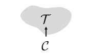
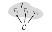
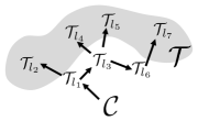
In many applications, the task-space manifold $\mathcal{T}$ is structured. In this paper, we consider the case where the task map $\psi$ can be expressed through a tree-structured composition of transformations $\{\psi_{e_{i}}\}$, where $\psi_{e_{i}}$ is the $i$th transformation. Fig. 1 illustrates some common examples, where each node denotes a manifold and each edge denotes a transformation. This family trivially includes the unstructured task space $\mathcal{T}$ (Fig. 1a) and the product manifold $\mathcal{T}=\mathcal{T}_{l_{1}}\times\dots\times\mathcal{T}_{l_{K}}$ (Fig. 1b), where $K$ is the number of subtasks. A more interesting example is the kinematic tree (Fig. 1c), where the task map considers the relationship between the configuration space $\mathcal{C}$ (the root node) and a collection of subtask spaces (the leaf nodes) that describe, e.g., the tracking and obstacle avoidance tasks along a multi-DOF robot.

The main motivation of explicitly handling the structure in the task map $\psi$ is two-fold. First, it allows RMPflow to exploit computation shared across different subtask maps. Second, it allows the user to focus on designing motion policies for each subtask individually, which is easier than directly designing a global policy for the entire task space $\mathcal{T}$. For example, $\mathcal{T}$ may describe the problem of humanoid walking, which includes staying balanced, scheduling contacts, and avoiding collisions. Directly parameterizing a policy to satisfy all these objectives can be daunting, whereas designing a policy for each subtask is more feasible.

IV-B Riemannian Motion Policies (RMPs)

Knowing the structure of the task map is not sufficient for consistently combining subtask policies: we require some information about the motion policies’ behaviors [17]. Toward this end, we adopt a more informative description of motion policies, called RMPs [17], for the nodes of the RMP-tree.

An RMP describes a second-order differential equation along with its geometric information on a smooth manifold. Specifically, let $\mathcal{M}$ be an $m$-dimensional manifold with coordinate $\mathbf{x}\in\mathbb{R}^{m}$. The canonical form of an RMP on $\mathcal{M}$ is a pair $(\mathbf{a},\mathbf{M})^{\mathcal{M}}$, where $\mathbf{a}:\mathbb{R}^{m}\times\mathbb{R}^{m}\to\mathbb{R}^{m}$ is a continuous motion policy and $\mathbf{M}:\mathbb{R}^{m}\times\mathbb{R}^{m}\to\mathbb{R}_{+}^{m\times m}$ is a differentiable map. Borrowing terminology from mechanics (cf. Section III-D), we call $\mathbf{a}(\mathbf{x},{\dot{\mathbf{x}}})$ the desired acceleration and $\mathbf{M}(\mathbf{x},{\dot{\mathbf{x}}})$ the inertia matrix at $(\mathbf{x},{\dot{\mathbf{x}}})$, respectively. For now, we can intuitively think that $\mathbf{M}$ defines the directional importance of $\mathbf{a}$ when it is combined with other motion policies. Later in Section V, we will show that $\mathbf{M}$ is closely related to the concept of Riemannian metric, which describes how the space is stretched along the curve generated by $\mathbf{a}$; when $\mathbf{M}$ depends on the state, the space becomes non-Euclidean.

In this paper, we additionally introduce a new RMP form, called the natural form. Given an RMP in its canonical form $(\mathbf{a},\mathbf{M})^{\mathcal{M}}$, we define another pair as its natural form $[\mathbf{f},\mathbf{M}]^{\mathcal{M}}$, where $\mathbf{f}=\mathbf{M}\mathbf{a}$ is the desired force map. While the transformation between these two forms may look trivial, their distinction will be useful later when we introduce the RMP-algebra.

IV-C RMP-tree

The RMP-tree is the core data structure used by RMPflow. An RMP-tree is a directed tree, in which each node represents an RMP and its state, and each edge corresponds to a transformation between manifolds. The root node of the RMP-tree describes the global policy $\pi$ on $\mathcal{C}$, and the leaf nodes describe the local policies $\{\pi_{l_{i}}\}$ on $\{\mathcal{T}_{l_{i}}\}$.

To illustrate, let us consider a node $u$ and its $K$ child nodes $\{v_{i}\}_{i=1}^{K}$. Suppose $u$ describes an RMP $[\mathbf{f},\mathbf{M}]^{\mathcal{M}}$ and $v_{i}$ describes an RMP $[\mathbf{f}_{i},\mathbf{M}_{i}]^{\mathcal{N}_{i}}$, where $\mathcal{N}_{i}=\psi_{e_{i}}(\mathcal{M})$ for some $\psi_{e_{i}}$. Then we write $u=((\mathbf{x},{\dot{\mathbf{x}}}),[\mathbf{f},\mathbf{M}]^{\mathcal{M}})$ and $v_{i}=((\mathbf{y}_{i},{\dot{\mathbf{y}}}_{i}),[\mathbf{f}_{i},\mathbf{M}_{i}]^{\mathcal{N}_{i}})$, where $(\mathbf{x},{\dot{\mathbf{x}}})$ is the state of $u$, and $(\mathbf{y}_{i},{\dot{\mathbf{y}}}_{i})$ is the state of $v_{i}$; the edge connecting $u$ and $v_{i}$ points from $u$ to $v_{i}$ along $\psi_{e_{i}}$. We will continue to use this example to illustrate how RMP-algebra propagates the information across the RMP-tree.

IV-D RMP-algebra

The RMP-algebra of RMPflow consists of three operators (pushforward, pullback, and resolve) to propagate information across the RMP-tree. They form the basis of the forward and backward passes for automatic policy generation, described in the next section.

1. pushforward is the operator to forward propagate the state from a parent node to its child nodes. Using the previous example, given $(\mathbf{x},{\dot{\mathbf{x}}})$ from $u$, it computes $(\mathbf{y}_{i},{\dot{\mathbf{y}}}_{i})=(\psi_{e_{i}}(\mathbf{x}),\mathbf{J}_{i}(\mathbf{x}){\dot{\mathbf{x}}})$ for each child node $v_{i}$, where $\mathbf{J}_{i}=\partial_{\mathbf{x}}\psi_{e_{i}}$ is a Jacobian matrix. The name “pushforward” comes from the linear transformation of tangent vector ${\dot{\mathbf{x}}}$ to the image tangent vector ${\dot{\mathbf{y}}}_{i}$.

2. pullback is the operator to backward propagate the natural-formed RMPs from the child nodes to the parent node. It is done by setting $[\mathbf{f},\mathbf{M}]^{\mathcal{M}}$ with

   $$\textstyle\mathbf{f}=\sum_{i=1}^{K}\mathbf{J}_{i}^{\top}(\mathbf{f}_{i}-\mathbf{M}_{i}\dot{\mathbf{J}}_{i}{\dot{\mathbf{x}}})\text{,\hskip 2.84526pt}\mathbf{M}=\sum_{i=1}^{K}\mathbf{J}_{i}^{\top}\mathbf{M}_{i}\mathbf{J}_{i}$$ (18)

   The name “pullback” comes from the linear transformations of the cotangent vector (1-form) $\mathbf{f}_{i}-\mathbf{M}_{i}\dot{\mathbf{J}_{i}}{\dot{\mathbf{x}}}$ and the inertia matrix (2-form) $\mathbf{M}_{i}$. In summary, velocities can be pushfowarded along the direction of $\psi_{i}$, and forces and inertial matrices can be pullbacked in the opposite direction.

   To gain more intuition of pullback, we write pullback in the canonical form of RMPs. It can be shown that the canonical form $(\mathbf{a},\mathbf{M})^{\mathcal{M}}$ of the natural form $[\mathbf{f},\mathbf{M}]^{\mathcal{M}}$ above is the solution to a least-squares problem (cf. Section III-E):

   $$\mathbf{a} =\textstyle\operatorname*{arg\,min}_{\mathbf{a}^{\prime}}\frac{1}{2}\sum_{i=1}^{K}\|\mathbf{J}_{i}\mathbf{a}^{\prime}+\dot{\mathbf{J}}_{i}{\dot{\mathbf{x}}}-\mathbf{a}_{i}\|_{\mathbf{M}_{i}}^{2}$$

   $$=\textstyle(\sum_{i=1}^{K}\mathbf{J}_{i}^{\top}\mathbf{M}_{i}\mathbf{J}_{i})^{\dagger}(\sum_{i=1}^{K}\mathbf{J}_{i}^{\top}\mathbf{M}_{i}(\mathbf{a}_{i}-\dot{\mathbf{J}}_{i}{\dot{\mathbf{x}}}))$$ (19)

   where $\mathbf{a}_{i}=\mathbf{M}_{i}^{\dagger}\mathbf{f}_{i}$ and $\|\cdot\|_{\mathbf{M}_{i}}^{2}=\left\langle\cdot,\mathbf{M}_{i}\cdot\right\rangle{\leavevmode\color[rgb]{0,0,0}=\cdot^{\top}\mathbf{M}_{i}\cdot}$. Because ${\ddot{\mathbf{y}}}_{i}=\mathbf{J}_{i}{\ddot{\mathbf{x}}}+\dot{\mathbf{J}}_{i}{\dot{\mathbf{x}}}$, pullback attempts to find an $\mathbf{a}$ that can realize the desired accelerations $\{\mathbf{a}_{i}\}$ while trading off approximation errors with an importance weight defined by the inertia matrix $\mathbf{M}_{i}(\mathbf{y}_{i},{\dot{\mathbf{y}}}_{i})$. The use of state dependent importance weights is a distinctive feature of RMPflow. It allows RMPflow to activate different RMPs according to both configuration and velocity (see Section IV-F for examples). Finally, we note that the pullback operator defined in this paper is slightly different from the original definition given in [17], which ignores the term $\dot{\mathbf{J}}_{i}{\dot{\mathbf{x}}}$ in (2). While ignoring $\dot{\mathbf{J}}_{i}{\dot{\mathbf{x}}}$ does not necessarily destabilize the system [32], its inclusion is critical to implement consistent policy behaviors.

3. resolve is the last operator of RMP-algebra. It maps an RMP from its natural form to its canonical form. Given $[\mathbf{f},\mathbf{M}]^{\mathcal{M}}$, it outputs $(\mathbf{a},\mathbf{M})^{\mathcal{M}}$ with $\mathbf{a}=\mathbf{M}^{\dagger}\mathbf{f}$, where $\dagger$ denotes Moore-Penrose inverse. The use of pseudo-inverse is because in general the inertia matrix is only positive semi-definite. Therefore, we also call the natural form of $[\mathbf{f},\mathbf{M}]^{\mathcal{M}}$ the unresolved form, as potentially it can be realized by multiple RMPs in the canonical form.

IV-E Algorithm: Motion Policy Generation

Now we show how RMPflow uses the RMP-tree and RMP-algebra to generate a global policy $\pi$ on $\mathcal{C}$. Suppose each subtask policy is provided as an RMP in the natural form. First, we construct an RMP-tree with the same structure as $\psi$, where we assign subtask RMPs as the leaf nodes and the global RMP $[\mathbf{f}_{r},\mathbf{M}_{r}]^{\mathcal{C}}$ as the root node. With the RMP-tree specified, RMPflow can perform automatic policy generation. At every time instance, it first performs a forward pass: it recursively calls pushforward from the root node to the leaf nodes to update the state information in each node in the RMP-tree. Second, it performs a backward pass: it recursively calls pullback from the leaf nodes to the root node to back propagate the values of the RMPs in the natural form. Finally, it calls resolve at the root node to transform the global RMP $[\mathbf{f}_{r},\mathbf{M}_{r}]^{\mathcal{C}}$ into its canonical form $(\mathbf{a}_{r},\mathbf{M}_{r})^{\mathcal{C}}$ for policy execution (i.e. setting $\pi(\mathbf{q},{\dot{\mathbf{q}}})=\mathbf{a}_{r}$).

The process of policy generation of RMPflow uses the tree structure for computational efficiency. For $K$ subtasks, it has time complexity $O(K)$ in the worst case (the case with a binary tree) as opposed to $O(K\log K)$ of a naive implementation which does not exploit the tree structure, when running on a serial computer. In general, any RMP-tree representing the same leaf task spaces is equivalent, although its computational properties may differ. For instance, any leaf has a unique path from the root defining a series of transforms the configuration space must go through to admit the leaf’s space. That leaf can, therefore, be separated from the tree and linked to the root with a single edge along which a single map defined as the composition of maps along that unique path acts. Restructuring an RMP-tree into a star-shaped topology (i.e. the flat structure depicted in Figure Fig. 1b) with all leaves linked directly to the root using this separation process may be more amenable to parallel computation than the original tree. Usually it would be more effective to separate out entire subtrees by linking them to the root with a single edge containing the composition of transforms along the unique path to that subtree’s root. Separate computational nodes can process these entire subtrees in parallel using the RMPflow algorithm, then pullback the resulting RMPs to the root using message passing. In general, there are many ways a tree can be equivalently restructured to admit the same task spaces, and choosing the right tree for a given computational architecture is a design choice.

Furthermore, all computations of RMPflow are carried out using matrix-multiplications, except for the final resolve call, because the RMPs are expressed in the natural form in pullback instead of the canonical form suggested originally in [17]. This design makes RMPflow numerically stable, as only one matrix inversion $\mathbf{M}_{r}^{\dagger}\mathbf{f}_{r}$ is performed at the root node with both $\mathbf{f}_{r}$ and $\mathbf{M}_{r}$ in the span of the same Jacobian matrix due to pullback.

IV-F Example RMPs

We give a quick overview of some RMPs useful in practice (see Appendix D of the technical report [20] for further discussion of these RMPs) We recall from (2) that $\mathbf{M}$ dictates the directional importance of an RMP.

IV-F1 Collision/joint limit avoidance

Barrier-type RMPs are examples that use velocity dependent inertia matrices, which can express importance as a function of robot heading (a property that traditional mechanical principles fail to capture). Here we demonstrate a collision avoidance policy in the 1D distance space $x=d(\mathbf{q})$ to an obstacle. Let $g(x,\dot{x})=w(x)u(\dot{x})>0$ for some functions $w$ and $u$. We consider a motion policy such that $m(x,\dot{x})\ddot{x}+\frac{1}{2}\dot{x}^{2}\partial_{x}g(x,\dot{x})=-\partial_{x}\Phi(x)-b\dot{x}$ and define its inertia matrix $m(x,\dot{x})=g(x,\dot{x})+\frac{1}{2}\dot{x}\partial_{\dot{x}}g(x,\dot{x})$, where $\Phi$ is a potential and $b>0$ is a damper. We choose $w(x)$ to increase as $x$ decreases (close to the obstacle), $u(\dot{x})$ to increase when $\dot{x}<0$ (moving toward the obstacle), and $u(\dot{x})$ to be constant when $\dot{x}\geq 0$. With this choice, the RMP can be turned off in pullback when the robot heads away from the obstacle. This motion policy is a GDS and $g$ is its metric (cf. Section V-A); the terms $\frac{1}{2}\dot{x}\partial_{\dot{x}}g(x,\dot{x})$ and $\frac{1}{2}\dot{x}^{2}\partial_{x}g(x,\dot{x})$ are due to non-Euclidean geometry and produce natural repulsive behaviors as the robot moves toward the obstacle, and little or no force when it starts to move away.

IV-F2 Target attractors

Designing an attractor policy is relatively straightforward. For a task space with coordinate $\mathbf{x}$, we can consider an inertia matrix $\mathbf{M}(\mathbf{x})\succ 0$ and a motion policy such that ${\ddot{\mathbf{x}}}=-\nabla{\widetilde{\Phi}}-\beta(\mathbf{x}){\dot{\mathbf{x}}}-\mathbf{M}^{-1}\bm{\xi}_{\mathbf{M}}$, where ${\widetilde{\Phi}}(\mathbf{x})\approx\|\mathbf{x}\|$ is a smooth attractor potential, $\beta(\mathbf{x})\geq 0$ is a damper, and $\bm{\xi}_{\mathbf{M}}$ is a curvature term due to $\mathbf{M}$. It can be shown that this differential equation is also a GDS [20, Appendix D].

IV-F3 Orientations

As RMPflow directly works with manifold objects, orientation controllers become straightforward to design, independent of the choice of coordinate (cf. Section V-D). For example, we can define RMPs on a robotic link’s surface in any preferred coordinate (e.g. in one or two axes attached to an arbitrary point) with the above described attractor to control the orientation.

V Theoretical Analysis of RMPflow

We investigate the properties of RMPflow when the child-node motion policies belong to a class of differential equations, which we call structured geometric dynamical systems (structured GDSs). We present the following results.

1. Closure: We show that the pullback operator retains a closure of structured GDSs. When the child-node motion policies are structured GDSs, the parent-node dynamics also belong to the same class.

2. Stability: Using the closure property, we provide sufficient conditions for the feedback policy of RMPflow to be stable. In particular, we cover a class of dynamics with velocity-dependent metrics that are new to the literature.

3. Invariance: As its name suggests, RMPflow is closely related to differential geometry. We show that RMPflow is intrinsically coordinate-free. This means that a set of subtask RMPs designed for one robot can be transferred to another robot while maintaining the same task-space behaviors.

Setup Below we consider the manifolds in the nodes of the RMP-tree to be finite-dimensional and smooth. Without loss of generality, for now we assume that each manifold can be described in a single chart (i.e. using a global coordinate), so that we can write down the equations concretely using finite-dimensional variables. This restriction will be removed when we presents the coordinate-free form in Section V-D. We also assume that all the maps are sufficiently smooth so the required derivatives are well defined. The proofs of this section can found in the Appendix B of the technical report [20].

V-A Geometric Dynamical Systems (GDSs)

We first define a new family of dynamics, called GDSs, useful to specify RMPs on manifolds. (Structured GDSs will be introduced shortly in the next section.) At a high-level, a GDS can be thought as a virtual mechanical system defined on a manifold with an inertia that depends on both configuration and velocity. Formally, let us consider an $m$-dimensional manifold $\mathcal{M}$ with chart $(\mathcal{M},\mathbf{x})$ (i.e. a coordinate system on $\mathcal{M}$). Let $\mathbf{G}:\mathbb{R}^{m}\times\mathbb{R}^{m}\to\mathbb{R}^{m\times m}_{+}$, $\mathbf{B}:\mathbb{R}^{m}\times\mathbb{R}^{m}\to\mathbb{R}^{m\times m}_{+}$, and $\Phi:\mathbb{R}^{m}\to\mathbb{R}$ be sufficiently smooth functions. We say a dynamical system on $\mathcal{M}$ is a GDS $(\mathcal{M},\mathbf{G},\mathbf{B},\Phi)$, if it satisfies the differential equation

$$\left(\mathbf{G}(\mathbf{x},{\dot{\mathbf{x}}})+\bm{\Xi}_{\mathbf{G}}(\mathbf{x},{\dot{\mathbf{x}}})\right){\ddot{\mathbf{x}}}+\bm{\xi}_{\mathbf{G}}(\mathbf{x},{\dot{\mathbf{x}}})$$

$$=-\nabla_{\mathbf{x}}\Phi(\mathbf{x})-\mathbf{B}(\mathbf{x},{\dot{\mathbf{x}}}){\dot{\mathbf{x}}},$$ (20)

where we define

$$\bm{\Xi}_{\mathbf{G}}(\mathbf{x},{\dot{\mathbf{x}}}) \coloneqq\textstyle\frac{1}{2}\sum_{i=1}^{m}\dot{x}_{i}\partial_{{\dot{\mathbf{x}}}}\mathbf{g}_{i}(\mathbf{x},{\dot{\mathbf{x}}})$$

$$\bm{\xi}_{\mathbf{G}}(\mathbf{x},{\dot{\mathbf{x}}}) \coloneqq\overset{\lower 1.00006pt\hbox{$\scriptscriptstyle\mathbf{x}$}}{\mathbf{G}}(\mathbf{x},{\dot{\mathbf{x}}}){\dot{\mathbf{x}}}-\frac{1}{2}\nabla_{\mathbf{x}}({\dot{\mathbf{x}}}^{\top}\mathbf{G}(\mathbf{x},{\dot{\mathbf{x}}}){\dot{\mathbf{x}}})$$

$$\overset{\lower 1.00006pt\hbox{$\scriptscriptstyle\mathbf{x}$}}{\mathbf{G}}(\mathbf{x},{\dot{\mathbf{x}}}) \coloneqq[\partial_{\mathbf{x}}\mathbf{g}_{i}(\mathbf{x},{\dot{\mathbf{x}}}){\dot{\mathbf{x}}}]_{i=1}^{m}$$

and $\mathbf{g}_{i}(\mathbf{x},{\dot{\mathbf{x}}})$ is the $i$th column of $\mathbf{G}(\mathbf{x},{\dot{\mathbf{x}}})$. We refer to $\mathbf{G}(\mathbf{x},{\dot{\mathbf{x}}})$ as the metric matrix, $\mathbf{B}(\mathbf{x},{\dot{\mathbf{x}}})$ as the damping matrix, and $\Phi(\mathbf{x})$ as the potential function which is lower-bounded. In addition, we call the term in front of ${\ddot{\mathbf{x}}}$ in (V-A),

$$\mathbf{M}(\mathbf{x},{\dot{\mathbf{x}}})\coloneqq\mathbf{G}(\mathbf{x},{\dot{\mathbf{x}}})+\bm{\Xi}_{\mathbf{G}}(\mathbf{x},{\dot{\mathbf{x}}}),$$ (21)

the inertia matrix of GDS $(\mathcal{M},\mathbf{G},\mathbf{B},\Phi)$, which can be asymmetric. When $\mathbf{M}(\mathbf{x},{\dot{\mathbf{x}}})$ is nonsingular, we say the GDS is non-degenerate. We will assume (V-A) is non-degenerate for now so that it uniquely defines a differential equation. The discussion on the general case is postponed to Appendix A.

In GDSs, $\mathbf{G}(\mathbf{x},{\dot{\mathbf{x}}})$ induces a metric of ${\dot{\mathbf{x}}}$, measuring its length as $\frac{1}{2}{\dot{\mathbf{x}}}^{\top}\mathbf{G}(\mathbf{x},{\dot{\mathbf{x}}}){\dot{\mathbf{x}}}$. When $\mathbf{G}(\mathbf{x},{\dot{\mathbf{x}}})$ depends on $\mathbf{x}$ and ${\dot{\mathbf{x}}}$, it also induces non-trivial curvature terms $\bm{\Xi}(\mathbf{x},{\dot{\mathbf{x}}})$ and $\bm{\xi}(\mathbf{x},{\dot{\mathbf{x}}})$. In a particular case when $\mathbf{G}(\mathbf{x},{\dot{\mathbf{x}}})=\mathbf{G}(\mathbf{x})$ (i.e. it depends on configuration only), the GDSs reduce to the widely studied simple mechanical systems (SMSs) in geometric mechanics [16] (see also (5))

$$\mathbf{M}(\mathbf{x}){\ddot{\mathbf{x}}}+\mathbf{C}(\mathbf{x},{\dot{\mathbf{x}}}){\dot{\mathbf{x}}}+\nabla_{\mathbf{x}}\Phi(\mathbf{x})=-\mathbf{B}(\mathbf{x},{\dot{\mathbf{x}}}){\dot{\mathbf{x}}}$$ (22)

where the Coriolis force $\mathbf{C}(\mathbf{x},{\dot{\mathbf{x}}}){\dot{\mathbf{x}}}$ can be shown equal to $\bm{\xi}_{\mathbf{G}}(\mathbf{x},{\dot{\mathbf{x}}})$. In this special case, we have $\mathbf{M}(\mathbf{x})=\mathbf{G}(\mathbf{x})$, i.e., the inertia matrix is the same as the metric matrix (this is exactly the finding in geometric mechanics discussed in Section III-D2). We will revisit the connection between GDSs and SMSs again in Section VI-A (and show why $\mathbf{C}(\mathbf{x},{\dot{\mathbf{x}}}){\dot{\mathbf{x}}}=\bm{\xi}_{\mathbf{G}}(\mathbf{x},{\dot{\mathbf{x}}})$) after the analysis of geometric properties of GDSs. For now, we can think of GDSs as generalization of SMSs to have inertia $\mathbf{G}(\mathbf{x},{\dot{\mathbf{x}}})$ and metric $\mathbf{M}(\mathbf{x},{\dot{\mathbf{x}}})$ that also change with velocity! This velocity-dependent extension is important and non-trivial. As discussed in earlier Section IV-F, it generalizes the dynamics of classical rigid-body systems, allowing the space to morph according to the velocity direction.

Finally, as its name hints, GDSs possess geometric properties. Particularly, when $\mathbf{G}(\mathbf{x},{\dot{\mathbf{x}}})$ is invertible, the left-hand side of (V-A) is related to a quantity $\mathbf{a}_{\mathbf{G}}={\ddot{\mathbf{x}}}+\mathbf{G}(\mathbf{x},{\dot{\mathbf{x}}})^{-1}(\bm{\Xi}_{\mathbf{G}}(\mathbf{x},{\dot{\mathbf{x}}}){\ddot{\mathbf{x}}}+\bm{\xi}_{\mathbf{G}}(\mathbf{x},{\dot{\mathbf{x}}}))$, known as the geometric acceleration (cf. Section V-D). (Therefore these terms must not be separated; e.g. $\mathbf{G}(\mathbf{x},{\dot{\mathbf{x}}}){\ddot{\mathbf{x}}}$ alone may not possess particular meaning.) In other words, we can think of (V-A) as setting $\mathbf{a}_{\mathbf{G}}$ along the negative natural gradient $-\mathbf{G}(\mathbf{x},{\dot{\mathbf{x}}})^{-1}\nabla_{\mathbf{x}}\Phi(\mathbf{x})$ while imposing damping $-\mathbf{G}(\mathbf{x},{\dot{\mathbf{x}}})^{-1}\mathbf{B}(\mathbf{x},{\dot{\mathbf{x}}}){\dot{\mathbf{x}}}$.

V-B Closure

Earlier, we argued vaguely that by tracking the geometry in pullback in (18) through propagating RMPs instead of just motion policies, the task properties can be preserved. Here, we formalize this consistency concept of RMPflow as a closure of differential equations, named structured GDSs. Structured GDSs augment GDSs with information on how the metric matrix $\mathbf{G}$ factorizes. We call such information a structure. Specifically, suppose $\mathbf{G}$ has a structure $\SS$ that factorizes $\mathbf{G}(\mathbf{x},{\dot{\mathbf{x}}})=\mathbf{J}(\mathbf{x})^{\top}\mathbf{H}(\mathbf{y},{\dot{\mathbf{y}}})\mathbf{J}(\mathbf{x})$, where $\mathbf{y}:\mathbf{x}\mapsto\mathbf{y}(\mathbf{x})\in\mathbb{R}^{n}$ and $\mathbf{H}:\mathbb{R}^{n}\times\mathbb{R}^{n}\to\mathbb{R}^{n\times n}_{+}$, and $\mathbf{J}(\mathbf{x})=\partial_{\mathbf{x}}\mathbf{y}$ is the Jacobian. We say a dynamical system on $\mathcal{M}$ is a structured GDS $(\mathcal{M},\mathbf{G},\mathbf{B},\Phi)_{\SS}$ if it satisfies the differential equation

$$\left(\mathbf{G}(\mathbf{x},{\dot{\mathbf{x}}})+\bm{\Xi}_{\mathbf{G}}(\mathbf{x},{\dot{\mathbf{x}}})\right){\ddot{\mathbf{x}}}+\bm{\eta}_{\mathbf{G};\SS}(\mathbf{x},{\dot{\mathbf{x}}})$$

$$=-\nabla_{\mathbf{x}}\Phi(\mathbf{x})-\mathbf{B}(\mathbf{x},{\dot{\mathbf{x}}}){\dot{\mathbf{x}}}$$ (23)

where $\bm{\eta}_{\mathbf{G};\SS}(\mathbf{x},{\dot{\mathbf{x}}})\coloneqq\mathbf{J}(\mathbf{x})^{\top}(\bm{\xi}_{\mathbf{H}}(\mathbf{y},{\dot{\mathbf{y}}})+(\mathbf{H}(\mathbf{y},\dot{\mathbf{y}})+\bm{\Xi}_{\mathbf{H}}(\mathbf{y},{\dot{\mathbf{y}}}))\dot{\mathbf{J}}(\mathbf{x},{\dot{\mathbf{x}}}){\dot{\mathbf{x}}})$. If we compare GDSs in (V-A) and structured GDSs in (V-B), the difference is that $\bm{\xi}_{\mathbf{G}}(\mathbf{x},{\dot{\mathbf{x}}})$ is now replaced by a different curvature term $\bm{\eta}_{\mathbf{G};\SS}(\mathbf{x},{\dot{\mathbf{x}}})$ that is defined by both the metric and factorization. In fact, GDSs are structured GDSs with a trivial structure (i.e. $\mathbf{y}=\mathbf{x}$). Also, one can easily show that structured GDSs reduce to GDSs (i.e. the structure offers no extra information) if $\mathbf{G}(\mathbf{x},{\dot{\mathbf{x}}})=\mathbf{G}(\mathbf{x})$, or if $n,m=1$. Given two structures, we say $\SS_{a}$ preserves $\SS_{b}$ if $\SS_{a}$ has the factorization (of $\mathbf{H}$) made by $\SS_{b}$. In Section V-D, we will show that structured GDSs are related to a geometric object, pullback connection, which turns out to be the coordinate-free version of pullback.

Below we show the closure property: when the children of a parent node are structured GDSs, the parent node defined by pullback is also a structured GDS with respect to the pullbacked structured metric matrix, damping matrix, and potentials. Without loss of generality, we consider again a parent node on $\mathcal{M}$ with $K$ child nodes on $\{\mathcal{N}_{i}\}_{i=1}^{K}$. We note that $\mathbf{G}_{i}$ and $\mathbf{B}_{i}$ can be functions of both $\mathbf{y}_{i}$ and ${\dot{\mathbf{y}}}_{i}$.

Theorem 1.

Let the $i$th child node follow $(\mathcal{N}_{i},\mathbf{G}_{i},\mathbf{B}_{i},\Phi_{i})_{\SS_{i}}$ and have coordinate $\mathbf{y}_{i}$. Let $\mathbf{f}_{i}=-\bm{\eta}_{\mathbf{G}_{i};\SS_{i}}-\nabla_{\mathbf{y}_{i}}\Phi_{i}-\mathbf{B}_{i}{\dot{\mathbf{y}}}_{i}$ and $\mathbf{M}_{i}=\mathbf{G}_{i}+\bm{\Xi}_{\mathbf{G}_{i}}$. If $[\mathbf{f},\mathbf{M}]^{\mathcal{M}}$ of the parent node is given by pullback with $\{[\mathbf{f}_{i},\mathbf{M}_{i}]^{\mathcal{N}_{i}}\}_{i=1}^{K}$ and $\mathbf{M}$ is non-singular, the parent node follows the pullback structured GDS $(\mathcal{M},\mathbf{G},\mathbf{B},\Phi)_{\SS}$, where $\mathbf{G}=\sum_{i=1}^{K}\mathbf{J}_{i}^{\top}\mathbf{G}_{i}\mathbf{J}_{i}$, $\mathbf{B}=\sum_{i=1}^{K}\mathbf{J}_{i}^{\top}\mathbf{B}_{i}\mathbf{J}_{i}$, $\Phi=\sum_{i=1}^{K}\Phi_{i}\circ\mathbf{y}_{i}$, $\SS$ preserves $\SS_{i}$, and $\mathbf{J}_{i}=\partial_{\mathbf{x}}\mathbf{y}_{i}$. In other words, the parent node is the RMP $(\mathbf{a},\mathbf{M})^{\mathcal{M}}$ where $\mathbf{M}=\sum_{i=1}^{K}\mathbf{J}_{i}^{\top}(\mathbf{G}_{i}+\bm{\Xi}_{\mathbf{G}_{i}})\mathbf{J}_{i}$ and

$$\textstyle\mathbf{a}=\left(\mathbf{G}+\bm{\Xi}_{\mathbf{G}}\right)^{\dagger}\left(-\bm{\eta}_{\mathbf{G};\SS}-\nabla_{\mathbf{x}}\Phi-\mathbf{B}{\dot{\mathbf{x}}}\right)$$

Particularly, if every $\mathbf{G}_{i}$ is velocity-free and the child nodes are GDSs, the parent node follows $(\mathcal{M},\mathbf{G},\mathbf{B},\Phi)$.

Theorem 1 shows structured GDSs are closed under pullback. It means that the differential equation of a structured GDS with a tree-structured task map can be computed by recursively applying pullback from the leaves to the root, because in each recursive step, the form of structured GDS is preserved by pullback. Particularly, when $\mathbf{G}$ is velocity-free, one can show that pullback also preserves GDSs. We summarize these properties below.

Corollary 1.

If all leaf nodes follow GDSs and $\mathbf{M}_{r}$ at the root node is nonsingular, then the root node follows $(\mathcal{C},\mathbf{G},\mathbf{B},\Phi)_{\SS}$ as recursively defined by Theorem 1.

V-C Stability

By the closure property above, we analyze the stability of RMPflow when the leaf nodes are (structured) GDSs. For compactness, we will abuse the notation to write $\mathbf{M}=\mathbf{M}_{r}$. Suppose $\mathbf{M}$ is nonsingular and let $(\mathcal{C},\mathbf{G},\mathbf{B},\Phi)_{\SS}$ be the resultant structured GDS at the root node. We consider a Lyapunov function candidate

$$\textstyle V(\mathbf{q},{\dot{\mathbf{q}}})=\frac{1}{2}{\dot{\mathbf{q}}}^{\top}\mathbf{G}(\mathbf{q},{\dot{\mathbf{q}}}){\dot{\mathbf{q}}}+\Phi(\mathbf{q})$$ (24)

and derive its rate using properties of structured GDSs.

Proposition 1.

For $(\mathcal{C},\mathbf{G},\mathbf{B},\Phi)_{\SS}$, it holds that $\dot{\mathbf{V}}(\mathbf{q},{\dot{\mathbf{q}}})=-{\dot{\mathbf{q}}}^{\top}\mathbf{B}(\mathbf{q},{\dot{\mathbf{q}}}){\dot{\mathbf{q}}}$.

Proposition 1 directly implies the stability of structured GDSs by invoking LaSalle’s invariance principle [48]. Here we summarize the result without proof.

Corollary 2.

For $(\mathcal{C},\mathbf{G},\mathbf{B},\Phi)_{\SS}$, if $\mathbf{G}(\mathbf{q},{\dot{\mathbf{q}}}),\mathbf{B}(\mathbf{q},{\dot{\mathbf{q}}})\succ 0$, the system converges to a forward invariant set $\mathcal{C}_{\infty}\coloneqq\{(\mathbf{q},{\dot{\mathbf{q}}}):\nabla_{\mathbf{q}}\Phi(\mathbf{q})=0,{\dot{\mathbf{q}}}=0\}$.

To show the stability of RMPflow, we need to further check when the assumptions in Corollary 2 hold. The condition $\mathbf{B}(\mathbf{q},{\dot{\mathbf{q}}})\succ 0$ is easy to satisfy: by Theorem 1, $\mathbf{B}(\mathbf{q},{\dot{\mathbf{q}}})$ has the form $\sum_{i=1}^{K}\mathbf{J}_{i}(\mathbf{q})^{\top}\mathbf{B}_{i}(\mathbf{x}_{i},{\dot{\mathbf{x}}}_{i})\mathbf{J}_{i}(\mathbf{q})$. Therefore, it automatically satisfies $\mathbf{B}(\mathbf{q},{\dot{\mathbf{q}}})\succeq 0$; to strictly ensure definiteness, we can copy $\mathcal{C}$ into an additional child node with a (small) positive-definite damping matrix. The condition on $\mathbf{G}(\mathbf{q},{\dot{\mathbf{q}}})\succ 0$ can be satisfied based on a similar argument about $\mathbf{B}(\mathbf{q},{\dot{\mathbf{q}}})$. In addition, we need to verify the assumption that $\mathbf{M}$ is nonsingular. Here we provide a sufficient condition. When satisfied, it implies the global stability of RMPflow in the sense of Corollary 2.

Theorem 2.

Suppose every leaf node is a GDS with a metric matrix in the form $\mathbf{R}(\mathbf{x})+\mathbf{L}(\mathbf{x})^{\top}\mathbf{D}(\mathbf{x},{\dot{\mathbf{x}}})\mathbf{L}(\mathbf{x})$ for differentiable functions $\mathbf{R}$, $\mathbf{L}$, and $\mathbf{D}$ satisfying $\mathbf{R}(\mathbf{x})\succeq 0$, $\mathbf{D}(\mathbf{x},{\dot{\mathbf{x}}})=\mathrm{diag}((d_{i}(\mathbf{x},\dot{y}_{i}))_{i=1}^{n})\succeq 0$, and $\dot{y}_{i}\partial_{\dot{y}_{i}}d_{i}(\mathbf{x},\dot{y}_{i})\geq 0$, where $\mathbf{x}$ is the coordinate of the leaf-node manifold and ${\dot{\mathbf{y}}}=\mathbf{L}{\dot{\mathbf{x}}}\in\mathbb{R}^{n}$. It holds $\bm{\Xi}_{\mathbf{G}}(\mathbf{q},{\dot{\mathbf{q}}})\succeq 0$. If further $\mathbf{G}(\mathbf{q},{\dot{\mathbf{q}}}),\mathbf{B}(\mathbf{q},{\dot{\mathbf{q}}})\succ 0$, then $\mathbf{M}\in\mathbb{R}^{d\times d}_{++}$, and the global RMP generated by RMPflow converges to the forward invariant set $\mathcal{C}_{\infty}$ in Corollary 2.

A particular condition in Theorem 2 is when all the leaf nodes with velocity dependent metric are 1D. Suppose $x\in\mathbb{R}$ is its coordinate and $g(x,\dot{x})$ is its metric matrix. The sufficient condition essentially boils down to $g(x,\dot{x})\geq 0$ and $\dot{x}\partial_{\dot{x}}g(x,\dot{x})\geq 0$. This means that, given any $x\in\mathbb{R}$, $g(x,0)=0$, $g(x,\dot{x})$ is non-decreasing when $\dot{x}>0$, and non-increasing when $\dot{x}<0$. This condition is satisfied by the collision avoidance policy in Section IV-F.

V-D Invariance

We now discuss the coordinate-free geometric properties of $(\mathcal{C},\mathbf{G},\mathbf{B},\Phi)_{\SS}$ generated by RMPflow. Due to space constraint, we only summarize the results. Here we assume that $\mathbf{G}$ is positive-definite.

We first introduce some additional notations for the coordinate-free analysis and give definitions of common differential geometric objects (please see, e.g., [49] for an excellent tutorial). For a manifold $\mathcal{C}$, we use $T\mathcal{C}$ to denote its tangent bundle (i.e. a manifold that describes the tangent spaces on the base manifold $\mathcal{C}$) and write $p_{T\mathcal{C}}:T\mathcal{C}\to\mathcal{C}$ to denote the bundle projection, which recovers the corresponding point on $\mathcal{C}$ (i.e. configuration) from a point on $T\mathcal{C}$ (a pair of position and the attached tangent vector). Specifically, suppose $(U,(\mathbf{q},\mathbf{v}))$ is a (local) chart on $T\mathcal{C}$ on a neighborhood $U$. Let $\{\frac{\partial}{\partial q_{i}},\frac{\partial}{\partial v_{i}}\}_{i=1}^{d}$ and $\{\mathrm{d}{q^{i}},\mathrm{d}{v^{i}}\}_{i=1}^{d}$ denote the induced frame field and coframe field on $T\mathcal{C}$ (i.e. the basis vector fields that characterize the tangent spaces and their dual spaces). For $s\in U$, we write $s$ in coordinate as $(\mathbf{q}(q),\mathbf{v}(s))$, if $\sum_{i=1}^{d}v_{i}(s)\frac{\partial}{\partial q_{i}}|_{q}\in T_{q}\mathcal{C}$, where $q=p_{T\mathcal{C}}(s)\in\mathcal{C}$. With abuse of notation, we also write $s=(\mathbf{q},\mathbf{v})$ for short unless clarity is lost. Similarly, a chart $(\tilde{U},(\mathbf{q},\mathbf{v},\mathbf{u},\mathbf{a}))$ can naturally be constructed on the double tangent bundle $TT\mathcal{C}$, where $\tilde{U}=p_{TT\mathcal{C}}^{-1}(U)$ and $p_{TT\mathcal{C}}:TT\mathcal{C}\to T\mathcal{C}$ is the bundle projection: we write $h=(\mathbf{q},\mathbf{v},\mathbf{u},\mathbf{a})\in TT\mathcal{C}$ if $\sum_{i=1}^{d}u_{i}(h)\frac{\partial}{\partial q_{i}}|_{s}+a_{i}(h)\frac{\partial}{\partial v_{i}}|_{s}\in T_{s}T\mathcal{C}$, where $s=p_{TT\mathcal{C}}(h)$. Under these notations, for a curve $q(t)$ on $\mathcal{C}$, we can write $\ddot{q}(t)\in TT\mathcal{C}$ in coordinate as $(\mathbf{q}(t),{\dot{\mathbf{q}}}(t),{\dot{\mathbf{q}}}(t),{\ddot{\mathbf{q}}}(t))$. Finally, we define a geometric object called affine connection, which defines how tangent spaces at different points on a manifold are related. Given Christoffel symbols $\Gamma_{i,j}^{k}$, an affine connection $\nabla$ on $TT\mathcal{C}$ is defined via $\textstyle\nabla_{\frac{\partial}{\partial s_{i}}}\frac{\partial}{\partial s_{j}}=\sum_{k=1}^{2d}\Gamma_{i,j}^{k}\frac{\partial}{\partial s_{k}}$, where $\frac{\partial}{\partial s_{i}}\coloneqq\frac{\partial}{\partial q_{i}}$ and $\frac{\partial}{\partial s_{i+d}}\coloneqq\frac{\partial}{\partial v_{i}}$ for $i=1,\dots,d$.

Using this new notation, we show that GDSs can be written in a coordinate-free manner in terms of affine connection. Let $T\mathcal{C}$ denote the tangent bundle of $\mathcal{C}$, which is a natural manifold to describe the state space. Precisely, we prove that a GDS on $\mathcal{C}$ can be expressed in terms of a unique, asymmetric affine connection ${}^{\scriptstyle G}{\nabla}$ that is compatible with a Riemannian metric $G$ (defined by $\mathbf{G}$) on $T\mathcal{C}$. It is important to note that $G$ is defined on $T\mathcal{C}$ not the original manifold $\mathcal{C}$. As the metric matrix in a GDS can be velocity dependent, we need a larger manifold.

Theorem 3.

Let $G$ be a Riemannian metric on $T\mathcal{C}$ such that, for $s=(q,v)\in T\mathcal{C}$, $G(s)=\sum_{i,j}G^{v}_{ij}(s)dq^{i}\otimes dq^{j}+G^{a}_{ij}dv^{i}\otimes dv^{j}$, where $G^{v}_{ij}(s)$ and $G^{a}_{ij}$ are symmetric and positive-definite, and $G^{v}_{ij}(\cdot)$ is differentiable. Then there is a unique affine connection ${}^{\scriptstyle G}{\nabla}$ that is compatible with $G$ and satisfies, $\Gamma_{i,j}^{k}=\Gamma_{ji}^{k}$, $\Gamma_{i,j+d}^{k}=0$, and $\Gamma_{i+d,j+d}^{k}=\Gamma_{j+d,i+d}^{k}$, for $i,j=1,\dots,d$ and $k=1,\dots,2d$. In coordinates, if $G_{ij}^{v}(\dot{q})$ is identified as $\mathbf{G}(\mathbf{q},{\dot{\mathbf{q}}})$, then $\mathrm{pr}_{3}(^{\scriptstyle G}{\nabla}_{\ddot{q}}\ddot{q})$ can be written as $\mathbf{a}_{\mathbf{G}}\coloneqq{\ddot{\mathbf{q}}}+\mathbf{G}(\mathbf{q},{\dot{\mathbf{q}}})^{-1}(\bm{\xi}_{\mathbf{G}}(\mathbf{q},{\dot{\mathbf{q}}})+\bm{\Xi}_{\mathbf{G}}(\mathbf{q},{\dot{\mathbf{q}}}){\ddot{\mathbf{q}}})$, where $\mathrm{pr}_{3}:(\mathbf{q},\mathbf{v},\mathbf{u},\mathbf{a})\mapsto\mathbf{u}$ is a projection.

We call $\mathrm{pr}_{3}(^{\scriptstyle G}{\nabla}_{\dot{q}}\dot{q})$ the geometric acceleration of $q(t)$ with respect to ${}^{\scriptstyle G}{\nabla}$. It is a coordinate-free object, because $\mathrm{pr}_{3}$ is defined independent of the choice of chart on $\mathcal{C}$. By Theorem 3, it is clear that a GDS can be written abstractly as

$$\mathrm{pr}_{3}(^{\scriptstyle G}{\nabla}_{\ddot{q}}\ddot{q})=(\mathrm{pr}_{3}\circ G^{\sharp}\circ F)(s)$$ (25)

where $F:s\mapsto-d\Phi(s)-B(s)$ defines the covectors due to the potential function and damping, and $G^{\sharp}:T^{*}T\mathcal{C}\to TT\mathcal{C}$ denotes the inverse of $G$. In coordinates, it reads as ${\ddot{\mathbf{q}}}+\mathbf{G}(\mathbf{q},{\dot{\mathbf{q}}})^{-1}(\bm{\xi}_{\mathbf{G}}(\mathbf{q},{\dot{\mathbf{q}}})+\bm{\Xi}_{\mathbf{G}}(\mathbf{q},{\dot{\mathbf{q}}}){\ddot{\mathbf{q}}})=-\mathbf{G}(\mathbf{q},{\dot{\mathbf{q}}})^{-1}(\nabla_{\mathbf{q}}\Phi(\mathbf{q})+\mathbf{B}(\mathbf{q},{\dot{\mathbf{q}}}){\dot{\mathbf{q}}})$, which is exactly (V-A).

Extending this result, we present a coordinate-free representation of RMPflow when the leaf-nodes are GDSs.

Theorem 4.

Suppose $\mathcal{C}$ is related to $K$ leaf-node task spaces by maps $\{\psi_{i}:\mathcal{C}\to\mathcal{T}_{i}\}_{i=1}^{K}$ and the $i$th task space $\mathcal{T}_{i}$ has an affine connection ${}^{\scriptstyle G_{i}}{\nabla}$ on $T\mathcal{T}_{i}$, as defined in Theorem 3, and a covector function $F_{i}$ defined by some potential and damping as described above. Let ${}^{\scriptstyle G}{\bar{\nabla}}=\sum_{i=1}^{K}T\psi_{i}^{*}{{}^{\scriptstyle G_{i}}{\nabla}}$ be the pullback connection, $G=\sum_{i=1}^{K}T\psi_{i}^{*}G_{i}$ be the pullback metric, and $F=\sum_{i=1}^{K}T\psi_{i}^{*}F_{i}$ be the pullback covector, where $T\psi_{i}^{*}:T^{*}T\mathcal{T}_{i}\to T^{*}T\mathcal{C}$. Then ${}^{\scriptstyle G}{\bar{\nabla}}$ is compatible with $G$, and $\mathrm{pr}_{3}(^{\scriptstyle G}{\bar{\nabla}}_{\ddot{q}}\ddot{q})=(\mathrm{pr}_{3}\circ G^{\sharp}\circ F)(s)$ can be written as ${\ddot{\mathbf{q}}}+\mathbf{G}(\mathbf{q},{\dot{\mathbf{q}}})^{-1}(\bm{\eta}_{\mathbf{G};\SS}(\mathbf{q},{\dot{\mathbf{q}}})+\bm{\Xi}_{\mathbf{G}}(\mathbf{q},{\dot{\mathbf{q}}}){\ddot{\mathbf{q}}})=-\mathbf{G}(\mathbf{q},{\dot{\mathbf{q}}})^{-1}(\nabla_{\mathbf{q}}\Phi(\mathbf{q})+\mathbf{B}(\mathbf{q},{\dot{\mathbf{q}}}){\dot{\mathbf{q}}})$. In particular, if $G$ is velocity-independent, then ${}^{\scriptstyle G}{\bar{\nabla}}=^{\scriptstyle G}{\nabla}$.

Theorem 4 says that the structured GDS $(\mathcal{C},\mathbf{G},\mathbf{B},\Phi)_{\SS}$ can be written abstractly, without coordinates, using the pullback of task-space covectors, metrics, and asymmetric affine connections (that are defined in Theorem 3). In other words, the recursive calls of pullback in the backward pass of RMPflow is indeed performing “pullback” of geometric objects. We can think that the leaf nodes define the asymmetric affine connections, and RMPflow performs pullback to pullback those connections onto $\mathcal{C}$ to define ${}^{\scriptstyle G}{\bar{\nabla}}$. Theorem 4 also shows, when $G$ is velocity-independent, the pullback of connection and the pullback of metric commutes. In this case, ${}^{\scriptstyle G}{\bar{\nabla}}=^{\scriptstyle G}{\nabla}$, which is equivalent to the classic Levi-Civita connection of $G$. The loss of commutativity in general is due to the asymmetric definition of the connection in Theorem 3, which however is necessary to derive a control law of acceleration, without further referring to higher-order time derivatives.

VI Operational Space Control and Geometric Mechanics in View of RMPflow

With the algorithm details and theoretical properties of RMPflow introduced, we now discuss more precisely how RMPflow is connected to and generalizes existing work in geometric mechanics and operational space control.

VI-A From Operational Space Control to RMPflow with GDSs

Our study of GDSs (introduced in Section V-A) is motivated by SMSs in geometric mechanics which describe the dynamics used in existing operational space control schemes (cf. Section III). Many formulations of mechanics exist, including Lagrangian mechanics [46] and the aforementioned Gauss’s principle of least constraint [13], and they are all equivalent, implicitly sharing the same mathematical structure. But among them, we find that geometric mechanics, which models physical systems as geodesic flow on Riemannian manifolds, is the most explicit one: it summarizes the system properties arising from the underlying manifold structure compactly, as Riemannian metrics, and connects to the broad mathematical tool set from Riemannian geometry.

These geometry-based insights provide us a way to generalize beyond the previous SMSs studied in [16] and then design GDSs, a family non-classical dynamical systems that, through the use of configuration-and-velocity dependent metrics, more naturally describe behaviors of robots desired for tasks in non-Euclidean spaces.

The proposed generalization preserves several nice features from SMSs to GDSs. As in SMSs, the properties of GDSs are captured by the metric matrix. For example, a GDS like a SMS possesses the natural conservation property of kinematic energy, i.e. it travels along a geodesic defined by $\mathbf{G}(\mathbf{x},{\dot{\mathbf{x}}})$ when there is no external perturbations due to $\Phi$ and $\mathbf{B}$. Note that $\mathbf{G}(\mathbf{x},{\dot{\mathbf{x}}})$ by definition may only be positive-semidefinite even when the system is non-degenerate; here we allow the geodesic to be defined for a degenerate metric, meaning a curve whose instant length measured by the (degenerate) metric is constant. This geometric feature is an important tool to establish the stability of GDSs in our analysis; We highlight this nice property below, which is a corollary of Proposition 1. Note that this property also hold for degenerate GDSs provided that differential equations satisfying (26) exist.

Corollary 3.

All GDSs in the form $(\mathcal{M},\mathbf{G},0,0)$ travel on geodesics defined by $\mathbf{G}$. That is, $\dot{K}(\mathbf{x},{\dot{\mathbf{x}}})=0$, where $K(\mathbf{x},{\dot{\mathbf{x}}})=\frac{1}{2}{\dot{\mathbf{x}}}^{\top}\mathbf{G}(\mathbf{x},{\dot{\mathbf{x}}}){\dot{\mathbf{x}}}$.

As we discussed earlier, these generalized metrics induce curvature terms $\bm{\Xi}_{\mathbf{G}}$ and $\bm{\xi}_{\mathbf{G}}$ that can be useful to design sensible motions for tasks in non-Euclidean spaces (cf. Section IV-F). As we showed GDSs are coordinate-free, these terms and behaviors arise naturally when traveling on geodesics that is defined by configuration-and-velocity dependent metrics. To gain more intuition about these curvature terms, we recall that the curvature term $\bm{\xi}_{\mathbf{G}}$ in GDSs is related to the Coriolis force in the SMSs. This is not surprising, as from the analysis in Section V-D we know that $\bm{\xi}_{\mathbf{G}}$ comes from the Christoffel symbols of the asymmetric connection in Theorem 3, just as the Coriolis force comes from the Christoffel symbols of Levi-Civita connection. Recall it is defined as

$$\bm{\xi}_{\mathbf{G}}(\mathbf{x},{\dot{\mathbf{x}}}) \coloneqq\textstyle\overset{\lower 1.00006pt\hbox{$\scriptscriptstyle\mathbf{x}$}}{\mathbf{G}}(\mathbf{x},{\dot{\mathbf{x}}}){\dot{\mathbf{x}}}-\frac{1}{2}\nabla_{\mathbf{x}}({\dot{\mathbf{x}}}^{\top}\mathbf{G}(\mathbf{x},{\dot{\mathbf{x}}}){\dot{\mathbf{x}}})$$

Now we show their relationship explicitly below.

Lemma 1.

Let $\Gamma_{ijk}=\frac{1}{2}(\partial_{x_{k}}G_{ij}+\partial_{x_{j}}G_{ik}-\partial_{x_{j}}G_{jk})$ be the Christoffel symbol of the first kind with respect to $\mathbf{G}(\mathbf{x},{\dot{\mathbf{x}}})$, where the subscript _ij denotes the $(i,j)$ element. Let $C_{ij}=\sum_{k=1}^{d}\dot{x}_{k}\Gamma_{ijk}$ and define $\mathbf{C}(\mathbf{x},{\dot{\mathbf{x}}})=(C_{ij})_{i,j=1}^{m}$. Then $\bm{\xi}_{\mathbf{G}}(\mathbf{x},{\dot{\mathbf{x}}})=\mathbf{C}(\mathbf{x},{\dot{\mathbf{x}}}){\dot{\mathbf{x}}}$.

Proof of Lemma 1.

Suppose $\bm{\xi}_{\mathbf{G}}=(\xi_{i})_{i=1}^{m}$. We can compare the two definitions and verify they are indeed equivalent:

$$\xi_{i} =\textstyle\sum_{j,k=1}^{d}\dot{x}_{j}\dot{x}_{k}\partial_{x_{j}}G_{ik}-\frac{1}{2}\sum_{j,k=1}^{d}\dot{x}_{j}\dot{x}_{k}\partial_{x_{i}}G_{jk}$$

$$=\textstyle\frac{1}{2}\sum_{j,k=1}^{d}\dot{x}_{j}\dot{x}_{k}\partial_{x_{k}}G_{ij}+\frac{1}{2}\sum_{j,k=1}^{d}\dot{x}_{j}\dot{x}_{k}\partial_{x_{j}}G_{ik}$$

$$\quad\textstyle-\frac{1}{2}\sum_{j,k=1}^{d}\dot{x}_{j}\dot{x}_{k}\partial_{x_{i}}G_{jk}=\left(\mathbf{C}(\mathbf{x},{\dot{\mathbf{x}}}){\dot{\mathbf{x}}}\right)_{i}\qed$$

Thus, we can think intuitively that GDSs modify the inertia and the Coriolis forces in SMSs so that the dynamical system can preserve a generalized notion of kinematic energy that is no-longer necessarily quadratic in velocity.

Finally, we note that the benefits of using configuration-and-velocity dependent metrics can also be understood from their connection to the weight matrices in least-squared problems. Recall from Section III that for SMSs, the inertia matrix (which is the same as the metric matrix according to geometric mechanics) forms the importance weight in the least-squared problem. In other words, we can view common operational space control schemes as implicitly combining policies with constant or configuration dependent importance weight matrix in the least-squared sense, which implies certain restriction on the richness of behaviors that it can generate. By contrast, RMPflow allows generally importance weight matrices to depend also on velocity in the least-square problems prescribed by (18), which combines RMPs from the child nodes as a RMP at the parent node in every level of the RMP-tree (cf. Section IV). When the polices come from (structured) GDSs, these weight matrices now again are inertia matrices and the geometric properties of GDSs lead to similar stability and convergence properties as their SMS predecessors. Thus, in a sense, we can view RMPflow as generalizing operational space control to consider also configuration-and-velocity dependent weights in policy generation, allowing more flexible trade-offs between different policies.

VI-B Relationship between RMPflow and Recursive Newton-Euler Algorithms

For readers familiar with robot dynamics, we remark that the forward-backward policy generation procedure of RMPflow is closely related to the algorithms [18] for computing forward dynamics (i.e. computing accelerations given forces) based on recursive Newton-Euler algorithm. Here we discuss their relationship.

In a summary, these classic algorithms compute the forward dynamics using following steps:

1. It propagates positions and velocities from the base to the end-effector.

2. It computes the Coriollis force by backward propagating the inverse dynamics of each link under the condition that the acceleration is zero.

3. It computes the (full/upper-triangular/lower-triangular) joint inertia matrix.

4. It solves a linear system of equations to obtain the joint acceleration.

In [18], they assume a recursive Newton-Euler algorithm (RNE) for inverse dynamics is given, and realize Step 1 and Step 2 above by calling the RNE subroutine. The computation of Step 3 depends on which part of the inertia matrix is computed. In particular, their Method 3 (also called the Composite-Rigid-Body Algorithm in [50, Chapter 6]) computes the upper triangle part of the inertia matrix by a backward propagation from the end-effector to the base.

RMPflow can also be used to compute forward dynamics, when we set the leaf-node policy as the constant inertia system on the body frame of each link and we set the transformation in the RMP-tree as the change of coordinates across of robot links. This works because we showed that when leaf-node policies are GDSs (which cover SMSs of rigid-body dynamics as a special case), the effective dynamics at the root node is the pullback GDS, which in this case is the effective robot dynamics defined by the inertia matrix of each link.

We can use this special case to compare RMPflow with the above procedure. We see that the forward pass of RMPflow is equivalent to Step 1, and the backward pass of RMPflow is equivalent of Step 2 and Step 3, and the final resolve operation is equivalent to Step 4.

Despite similarity, the main difference is that RMPflow computes the force and the inertia matrix in a single backward pass to exploit shared computations. This change is important, especially, the number of subtasks are large, e.g., in avoiding multiples obstacles. In addition, the design of RMPflow generalizes these classical computational procedures (e.g. designed only for rigid bodies, rotational/prismatic joints) to handle abstract and even non-Euclidean task spaces that have velocity-dependent metrics/inertias. This extension provides a unified framework of different algorithms and results in an expressive class of motion policies.

Finally, we note that the above idea can be slightly modified so that we can also use RMPflow to compute the inverse dynamics. This can be done similarly to the above construction using physical inertia to initialize leaf-node RMPs; but at the end, after the backward pass, we solve for instead the torque as $\bm{\tau}=\mathbf{M}_{r}{\ddot{\mathbf{q}}}_{d}-\mathbf{M}_{r}\mathbf{f}_{r}$ where ${\ddot{\mathbf{q}}}_{d}$ is the desired joint-space acceleration.

VI-C Related Approaches to Motion Policy Generation

While here we focus on the special case of RMPflow with GDSs, this family already covers a wide range of reactive policies commonly used in practice. For example, when the task metric is Euclidean (i.e. constant), RMPflow recovers operational space control (and its variants) [10, 31, 11, 12, 32]. When the task metric is only configuration dependent, RMPflow can be viewed as performing energy shaping to combine multiple SMSs in geometric control [16]. Further, RMPflow allows using velocity dependent metrics, generating behaviors all those previous rigid mechanics-based approaches fail to model. We also note that RMPflow can be easily modified to incorporate exogenous time-varying inputs (e.g. forces to realize impedance control [30] or learned perturbations as in DMPs [44]). In computation, the structure of RMPflow in natural-formed RMPs resembles the classical Recursive Newton-Euler algorithm [18, 50] (as we just discussed above). Alternatively, the canonical form of RMPflow in (2) resembles Gauss’s Principle [11, 12], but with a curvature correction $\bm{\Xi}_{\mathbf{G}}$ on the inertia matrix (suggested by Theorem 1) to account for velocity dependent metrics. Thus, we can view RMPflow as a natural generalization of these approaches to a broader class of non-Euclidean behaviors.

VII Experiments

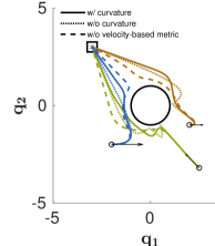
We first perform controlled experiments to study the curvature effects of nonlinear metrics, which is important for stability and collision avoidance. Then we conduct several full-body experiments (video: https://youtu.be/Fl4WvsXQDzo) to demonstrate the capabilities of RMPflow on high-DOF manipulation problems in clutter, and implement an integrated vision-and-motion system on two physical robots. Extra details of the RMPs used in this section can found in the Appendix D of the technical report [20].

(a)

(b)

(c)

(d)

Figure 2: Phase portraits (gray) and integral curves (blue; from black circles to red crosses) of 1D example. (a) Desired behavior. (b) With curvature terms. (c) Without curvature terms. (d) Without curvature terms but with nonlinear damping.

(a)

(b)

(c)

(d)

(e)

(f)

Figure 3: 2D example; initial positions (small circle) and velocities (arrows). (a-d) Obstacle (circle) avoidance: (a) w/o curvature terms and w/o potential. (b) w/ curvature terms and w/o potential. (c) w/o curvature terms and w/ potential. (d) w/ curvature terms and w/ potential. (e) Combined obstacle avoidance and goal (square) reaching. (f) The change of Lyapunov function in (24) over time along the trajectories in (e).

VII-A Controlled Experiments

VII-A1 1D Example

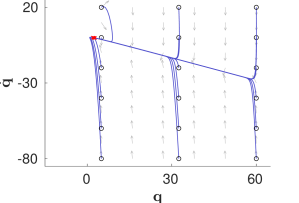
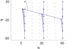
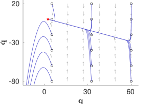
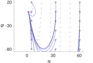
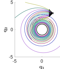
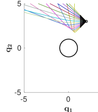
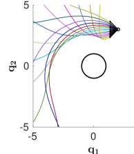
Let $\mathbf{q}\in\mathbb{R}$. We consider a barrier-type task map $\mathbf{x}=1/\mathbf{q}$ and define a GDS in (V-A) with $\mathbf{G}=1$, $\Phi(\mathbf{x})=\frac{1}{2}(\mathbf{x}-\mathbf{x}_{0})^{2}$, and $\mathbf{B}=(1+1/\mathbf{x})$, where $\mathbf{x}_{0}>0$. Using the GDS, we can define an RMP $[-\nabla_{\mathbf{x}}\Phi-\mathbf{B}{\dot{\mathbf{x}}}-\bm{\xi}_{\mathbf{G}},\mathbf{M}]^{\mathbb{R}}$, where $\mathbf{M}$ and $\bm{\xi}_{\mathbf{G}}$ are defined according to Section V-A. We use this example to study the effects of $\dot{\mathbf{J}}{\dot{\mathbf{q}}}$ in pullback (18), where we define $\mathbf{J}=\partial_{\mathbf{q}}\mathbf{x}$. Fig. 2 compares the desired behavior (Fig. 2a) and the behaviors of correct/incorrect pullback. If pullback is performed correctly with ${\dot{\mathbf{J}}}{\dot{\mathbf{q}}}$, the behavior matches the designed one (Fig. 2b). By contrast, if ${\dot{\mathbf{J}}}{\dot{\mathbf{q}}}$ is ignored, the observed behavior becomes inconsistent and unstable (Fig. 2c). While the instability of neglecting $\dot{\mathbf{J}}{\dot{\mathbf{q}}}$ can be recovered with a damping $\mathbf{B}=(1+\frac{{\dot{\mathbf{x}}}^{2}}{\mathbf{x}})$ nonlinear in ${\dot{\mathbf{x}}}$ (suggested in [32]), the behavior remains inconsistent (Fig. 2d).

VII-A2 2D Example

We consider a 2D goal-reaching task with collision avoidance and study the effects of velocity dependent metrics. First, we define an RMP (a GDS as in Section IV-F) in $\mathbf{x}=d(\mathbf{q})$ (the 1D task space of the distance to the obstacle). We pick a metric $\mathbf{G}(\mathbf{x},{\dot{\mathbf{x}}})=w(\mathbf{x})u({\dot{\mathbf{x}}})$, where $w(\mathbf{x})=1/\mathbf{x}^{4}$ increases if the particle is close to the obstacle and $u({\dot{\mathbf{x}}})=\epsilon+\min(0,{\dot{\mathbf{x}}}){\dot{\mathbf{x}}}$ (where $\epsilon\geq 0$), increases if it moves towards the obstacle. As this metric is non-constant, the GDS has curvature terms $\bm{\Xi}_{\mathbf{G}}=\frac{1}{2}{\dot{\mathbf{x}}}w(\mathbf{x})\partial_{\dot{\mathbf{x}}}u({\dot{\mathbf{x}}})$ and $\bm{\xi}_{\mathbf{G}}=\frac{1}{2}{\dot{\mathbf{x}}}^{2}u({\dot{\mathbf{x}}})\partial_{\mathbf{x}}w(\mathbf{x})$. These curvature terms along with ${\dot{\mathbf{J}}}{\dot{\mathbf{q}}}$ produce an acceleration that lead to natural obstacle avoidance behavior, coaxing the system toward isocontours of the obstacle (Fig. 3b). On the other hand, when the curvature terms are ignored, the particle travels in straight lines with constant velocity (Fig. 3a). To define the full collision avoidance RMP, we introduce a barrier-type potential $\Phi(\mathbf{x})=\frac{1}{2}\alpha w(\mathbf{x})^{2}$ to create extra repulsive forces, where $\alpha\geq 0$. A comparison of the curvature effects in this setting is shown in Fig. 3c and 3d (with $\alpha=1$). Next, we use RMPflow to combine the collision avoidance RMP above (with $\alpha=0.001$) and an attractor RMP. Let $\mathbf{q}_{g}$ be the goal. The attractor RMP is a GDS in the task space $\mathbf{y}=\mathbf{q}-\mathbf{q}_{g}$ with a metric $w(\mathbf{y})\mathbf{I}$, a damping $\eta w(\mathbf{y})\mathbf{I}$, and a potential that is zero at $\mathbf{y}=0$, where $\eta>0$ (see [20, Appendix D]). Fig. 3e shows the trajectories of the combined RMP. The combined non-constant metrics generate a behavior that transitions smoothly towards the goal while heading away from the obstacle. When the curvature terms are ignored (for both RMPs), the trajectories oscillate near the obstacle. In practice, this can result in jittery behavior on manipulators. When the metric is not velocity-based ($\mathbf{G}(\mathbf{x})=w(\mathbf{x})$) the behavior is less efficient in breaking free from the obstacle to go toward the goal. Finally, we show the change of Lyapunov function (24) over time along these trajectories in Fig. 3f as verification of our theory.

VII-B System Experiments

Figure 4: This figure depicts the tree of task maps used in the experiments. See Section VII-B1 for details.

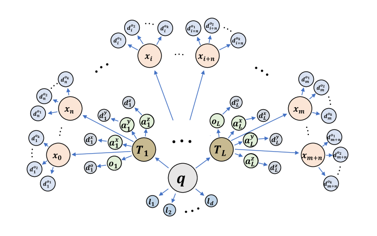
VII-B1 Task map and its Tree Structure

Fig. 4 depicts the tree of task maps used in the full-robot experiments. The chosen structure emphasizes potential for parallelization over fully exploiting the recursive nature of the kinematic chain, treating each link frame as just one forward kinematic map step from the configuration space. The configuration space $\mathbf{q}$ is linked to $L$ link frames $\mathbf{T}_{1},\ldots,\mathbf{T}_{L}$ through the robot’s forward kinematics (the details of tasks will be described later on for each individual experiment). Each frame has 4 frame element spaces: the origin $o_{i}$ and each of the axes $\mathbf{a}_{i}^{x},\mathbf{a}_{i}^{y},\mathbf{a}_{i}^{z}$, with corresponding distance spaces to targets $d_{i}^{o},d_{i}^{x},d_{i}^{y},d_{i}^{z}$ (if they are active). Additionally, there are a number of obstacle control points $\mathbf{x}_{j}$ distributed across each of the links, each with $k$ associated distance spaces $d_{j}^{o_{1}},\ldots,d_{j}^{o_{k}}$, one for each obstacle $o_{1},\ldots,o_{k}$. Finally, for each dimension of the configuration space there’s an associated joint limit space $l_{1},\ldots,l_{d}$.

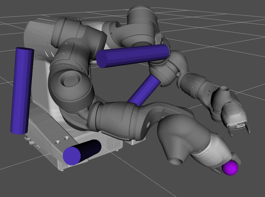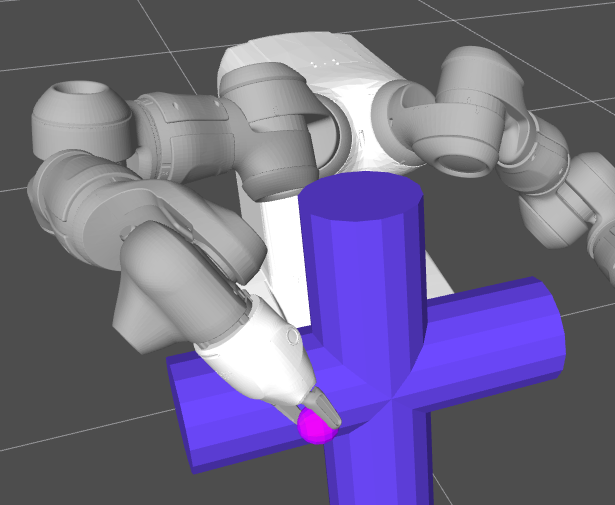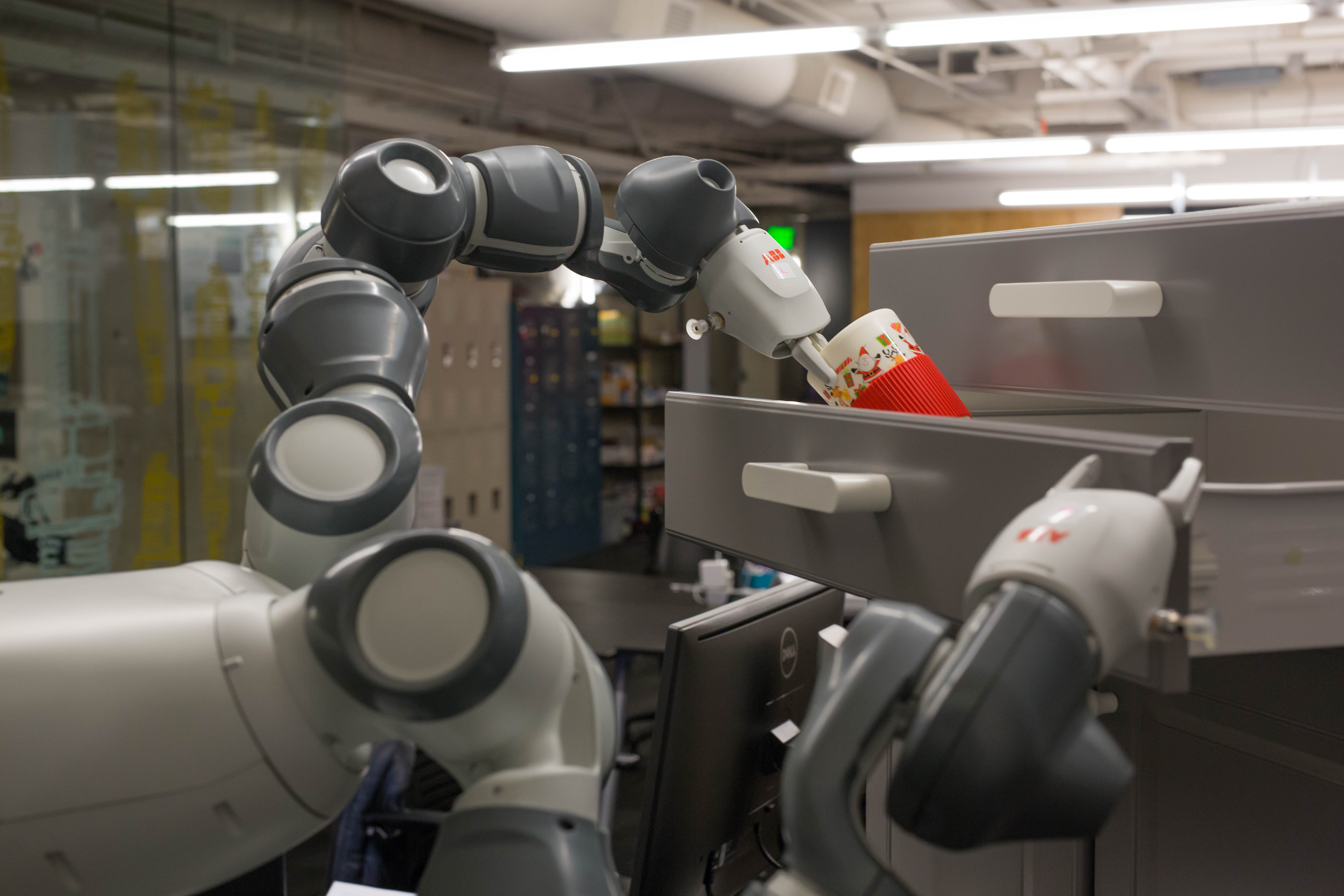simulated worlds		real-world experiments

Figure 5: Two of the six simulated worlds in the reaching experiments (left), and the two physical dual-arm platforms in the full system experiment (right).

Figure 6: Results for reaching experiments. Though some methods achieve a shorter goal distance than RMPflow in successful trials, they end up in collision in most the trials.

VII-B2 Reaching-through-clutter Experiments

We set up a collection of clutter-filled environments with cylindrical obstacles of varying sizes in simulation as depicted in Fig. 5, and tested the performance of RMPflow and two potential field methods on a modeled ABB YuMi robot.

Compared methods:

1. RMPflow: We implement RMPflow using the RMPs in Section IV-F and detailed in [20, Appendix D]. In particular, we place collision-avoidance controllers on distance spaces $s_{ij}=d_{j}(\mathbf{x}_{i})$, where $j=1,\ldots,m$ indexes the world obstacle $o_{j}$ and $i=1,\ldots,n$ indexes the $n$ control point along the robot’s body. Each collision-avoidance controller uses a weight function $w_{o}(\mathbf{x})$ that ranges from $0$ when the robot is far from the obstacle to $w_{o}^{\mathrm{max}}\gg 0$ when the robot is in contact with the obstacle’s surface. Similarly, the attractor potential uses a weight function $w_{a}(\mathbf{x})$ that ranges from $w_{a}^{\mathrm{min}}$ far from the target to $w_{a}^{\mathrm{max}}$ close to the target.

2. PF-basic: This variant is a basic implementation of obstacle avoidance potential fields with dynamics shaping. We use the RMP framework to implement this variant by placing collision-avoidance controllers on the same body control points used in RMPflow but with isotropic metrics of the form $\mathbf{G}_{o}^{\mathrm{basic}}(\mathbf{x})=w_{o}^{\mathrm{max}}\mathbf{I}$ for each control point, with $w_{o}^{\mathrm{max}}$ matching the value RMPflow uses. Similarly, the attractor uses the same attractor potential as RMPflow, but with a constant isotropic metric with the form $\mathbf{G}_{a}^{\mathrm{basic}}(\mathbf{x})=w_{a}^{\mathrm{max}}\mathbf{I}$.

3. PF-nonlinear: This variant matches PF-basic in construction, except it uses a nonlinear isotropic metrics of the form $\mathbf{G}_{o}^{\mathrm{nlin}}(\mathbf{x}_{i})=w_{o}(\mathbf{x})\mathbf{I}$ and $\mathbf{G}_{a}^{\mathrm{nlin}}(\mathbf{x}_{i})=w_{a}(\mathbf{x})\mathbf{I}$ for obstacle-avoidance and attraction, respectively, using weight functions matching RMPflow.

A note on curvature terms: PF-basic uses constant metrics, so has no curvature terms; PF-nonlinear has nontrivial curvature terms arising from the spatially varying metrics, but we ignore them here to match common practice from the operational space control literature.

Parameter scaling of PF-basic: Isotropic metrics do not express spacial directionality toward obstacles, and that leads to an inability of the system to effectively trade off the competing controller requirements. That conflict results in more collisions and increased instability. We, therefore, compare PF-basic under these baseline metric weights (matching RMPflow) with variants that incrementally strengthen collision avoidance controllers and C-space postural controllers ($f_{\mathcal{C}}(\mathbf{q},{\dot{\mathbf{q}}})=\gamma_{p}(\mathbf{q}_{0}-\mathbf{q})-\gamma_{d}{\dot{\mathbf{q}}}$) to improve these performance measures in the experiment. We use the following weight scalings (first entry denotes the obstacle metric scalar, and the second entry denotes the C-space metric scalar): “low” $(3,10)$, “med” $(5,50)$, and “high” $(10,100)$.

Environments: We run each of these variants on $6$ obstacle environments with $20$ randomly sampled target locations each distributed on the opposite side of the obstacle field from the robot. Three of the environments use four smaller obstacles (depicted in panel 3 of Fig. 5), and the remaining three environments used two large obstacles (depicted in panel 4 of Fig. 5). Each environment used the same $20$ targets to avoid implicit sampling bias in target choice.

Performance measures: We report results in Fig. 6 in terms of mean and one standard deviation error bars calculated across the $120$ trials for each of the following performance measures:

1. Time to goal (“time”): Length of time, in seconds, it takes for the robot to reach a convergence state. This convergence state is either the target, or its best-effort local minimum. If the system never converges, as in the case of many potential field trials for infeasible problems, the trial times out after 5 seconds. This metric measures time-efficiency of the movement.

2. C-space path length (“length”): This is the total path length $\int\|{\dot{\mathbf{q}}}\|dt$ of the movement through the configuration space across the trial. This metric measures how economical the movement is. In many of the potential-field variants with lower weights, we see significant fighting among the controllers resulting in highly inefficient extraneous motions.

3. Minimal achievable distance to goal (“goal distance”): Measures how close, in meters, the system is able to get to the goal with its end-effector.

4. Percent time in collision for colliding trials (“collision intensity”): Given that a trial has a collision, this metric measures the fraction of time the system is in collision throughout the trial. This metric indicates the intensity of the collision. Low values indicate short grazing collisions while higher values indicate long term obstacle penetration.

5. Fraction of trails with collisions (“collision failure”): Reports the fraction of trials with any collision event. We consider these to be collision-avoidance controller failures.

Discussion: In Fig. 6, we see that RMPflow outperforms each of these variants significantly, with some informative trends:

1. RMPflow never collides, so its collision intensity and collision failure values are $0$.

2. The other techniques, progressing from no scaling of collision-avoidance and C-space controller weights to substantial scaling, show a profile of substantial collision in the beginning to fewer (but still non-zero) collision events in the end. But we note that improvement in collision-avoidance is achieved at the expense of time-efficiency and the robot’s ability to reach the goal (it is too conservative).

3. Lower weight scaling of both PF-basic and PF-nonlinear actually achieve some faster times and better goal distances, but that is because the system pushes directly through obstacles, effectively “cheating” during the trial. RMPflow remains highly economical with its best effort reaching behaviors while ensuring the trials remain collision-free.

4. Lower weight scalings of PF-basic are highly uneconomical in their motion reflective of their relative instability. As the C-space weights on the posture controllers increase, the stability and economy of motion increase, but, again, at the expense of time-efficiency and optimality of the final reach.

5. There is little empirical difference between PF-basic and PF-nonlinear indicating that the defining feature separating RMPflow from the potential field techniques is its use of a highly nonlinear metric that explicitly stretches the space in the direction of the obstacle as well as in the direction of the velocity toward the target. Those stretchings penalize deviations in the stretched directions during combination with other controllers while allowing variation along orthogonal directions. By being more explicit about how controllers should instantaneously trade off with one another, RMPflow is better able to mitigate the otherwise conflicting control signals.

Summary: Isotropic metrics do not effectively convey how each collision and attractor controller should trade off with one another, resulting in a conflict of signals that obscure the intent of each controller making simultaneous collision avoidance, attraction, and posture maintenance more difficult. Increasing the weights of the controllers can improve their effectiveness, but at the expense of decreased overall system performance. The resulting motions are slower and less effective in reaching the goal in spite of more stable behavior and fewer collisions. A key feature of RMPflow is its ability to leverage highly nonlinear metrics that better convey information about how controllers should trade off with one another, while retaining provable stability guarantees. In combination, these features result in efficient and economical obstacle avoidance behavior while reaching toward targets amid clutter.

VII-B3 System Integration for Real-Time Reactive Motion Generation

We demonstrate the integrated vision and motion system on two physical dual arm manipulation platforms: a Baxter robot from Rethink Robotics, and a YuMi robot from ABB. Footage of our fully integrated system (see start of Section VII for the link) depicting tasks such as pick and place amid clutter, reactive manipulation of a cabinet drawers and doors with human interaction, active leadthrough with collision controllers running, and pick and place into a cabinet drawer.

This full integrated system, shown in the supplementary video, uses the RMPs described in Section IV-F (detailed in [20, Appendix D]) with a slight modification that the curvature terms are ignored. Instead, we maintain theoretical stability by using sufficient damping terms as described in Section VII-A and by operating at slower speeds. Generalization of these RMPs between embodiments was anecdotally pretty consistent, although, as we demonstrate in our experiments, we would expect more empirical deviation at higher speeds. For these manipulation tasks, this early version of the system worked well as demonstrated in the video.

For visual perception, we leveraged consumer depth cameras along with two levels of perceptual feedback:

1. Ambient world: For the Baxter system we create a voxelized representation of the unmodeled ambient world, and use distance fields to focus the collision controllers on just the closest obstacle points surrounding the arms. This methodology is similar in nature to [14], except we found empirically that attending to only the closest point to a skeleton representation resulted in oscillation in concaved regions where distance functions might result in nonsmooth kinks. We mitigate this issue by finding the closest points to a volume around each control point, effectively smoothing over points of nondifferentiability in the distance field.

2. Tracked objects: We use the Dense Articulated Real-time Tracking (DART) system of [51] to track articulated objects in real time through manipulations. This system is able to track both the robot and environmental objects, such as an articulated cabinet, simultaneously to give accurate measurements of their relative configuration effectively obviating the need for explicit camera-world calibration. As long as the system is initialized in the general region of the object locations (where for the cabinet and the robot, that would mean even up to half a foot of error in translation and a similar scale of error in rotation), the DART optimizer will snap to the right configuration when turned on. DART sends information about object locations to the motion generation, and receives back information about expected joint configurations (priors) from the motion system generating a robust world representation usable in a number of practical real-world manipulation problems.

Each of our behaviors are decomposed as state machines that use visual feedback to detect transitions, including transitions to reaction states as needed to implement behavioral robustness. Each arm is represented as a separate robot for efficiency, receiving real-time information about other arm’s current state enabling coordination. Both arms are programmed simultaneously using a high level language that provides the programmer a unified view of the surrounding world and command of both arms.

VIII Conclusion

We propose an efficient policy synthesis framework, RMPflow, for generating policies with non-Euclidean behavior, including motion with velocity dependent metrics that are new to the literature. In design, RMPflow is implemented as a computational graph, which can geometrically consistently combine subtask policies into a global policy for the robot. In theory, we provide conditions for stability and show that RMPflow is intrinsically coordinate-free. In the experiments, we demonstrate that RMPflow can generate smooth and natural motion for various tasks, when proper subtask RMPs are specified. Future work is to further relax the requirement on the quality of designing subtask RMPs by introducing learning components into RMPflow for additional flexibility.

Appendix A Degenerate GDSs

We discuss properties of degenerate GDSs. Let us recall the GDS $(\mathcal{M},\mathbf{G},\mathbf{B},\Phi)$ means the differential equation

$$\mathbf{M}(\mathbf{x},{\dot{\mathbf{x}}}){\ddot{\mathbf{x}}}+\bm{\xi}_{\mathbf{G}}(\mathbf{x},{\dot{\mathbf{x}}})=-\nabla_{\mathbf{x}}\Phi(\mathbf{x})-\mathbf{B}(\mathbf{x},{\dot{\mathbf{x}}}){\dot{\mathbf{x}}}$$ (26)

where $\mathbf{M}(\mathbf{x},{\dot{\mathbf{x}}})=\mathbf{G}(\mathbf{x},{\dot{\mathbf{x}}})+\bm{\Xi}_{\mathbf{G}}(\mathbf{x},{\dot{\mathbf{x}}})$. For degenerate cases, $\mathbf{M}(\mathbf{x},{\dot{\mathbf{x}}})$ can be singular and (26) define rather a family of differential equations. Degenerate cases are not uncommon; for example, the leaf-node dynamics could have $\mathbf{G}$ being only positive semidefinite. Having degenerate GDSs does not change the properties that we have proved, but one must be careful about whether differential equation satisfying (26) exist. For example, the existence is handled by the assumption on $\mathbf{M}$ in Theorem 1 and the assumption on $\mathbf{M}_{r}$ in Corollary 1. For RMPflow, we only need that $\mathbf{M}_{r}$ at the root node is non-singular. In other words, the natural-form RMP created by pullback at the root node can be resolved in the canonical-form RMP for policy execution. A sufficient and yet practical condition is provided in Theorem 2.

Ching-An Cheng is a Robotics Ph.D. student at Institute for Robotics and Intelligent Machines, Georgia Tech. Previously he received M.S. in Mechanical Engineering, B.S. in Electrical Engineering, and B.S. in Mechanical Engineering from National Taiwan University. He is interested in developing theoretical foundations toward efficient and principled robot learning. His research concerns sample efficiency, structural properties, and uncertainties in reinforcement/imitation learning, online learning, and integrated motion planning and control.

Mustafa Mukadam is a Ph.D. student in Robotics at Georgia Institute of Technology and a member of the Institute for Robotics and Intelligent Machines. Previously, he received his M.S. degree in Aerospace Engineering from University of Illinois at Urbana-Champaign. His research focuses on motion planning, learning from demonstration, estimation, and structured techniques to bridge robotics and machine learning, with applications in autonomous navigation and mobile manipulation.

Jan Issac is a software engineer at Nvidia with extensive experience API design, in low level, and high level programming applied in complex systems such as humanoid robotics. Jan studied computer science at Kalrsruhe Institute of Technology (KIT) Germany and Royal Institute of Technology (KTH) Stockholm, Sweden. He did his final thesis on stochastic filtering for high dimensional on-line object tracking at Computational Learning and Motor Control Lab (CLMC) at University of Southern California (USC), Los Angeles, and Max Planck Institute of Intelligent Systems - Autonomous Motion Department (AMD MPI-IS), Germany. He co-founded Lula Robotics and helped design and build the system which is now central to Nvidia’s manipulation research. He earned his Diploma (M.Sc.) in computer science from KIT in 2014.

Stan Birchfield is a principal research scientist at NVIDIA, exploring the intersection of computer vision and robotics. Previously, he was a tenured professor at Clemson University, where he led research in computer vision, visual tracking, mobile robotics, and the perception of highly deformable objects. He remains an adjunct faculty member at Clemson. He has also conducted research at Microsoft, was the principal architect of a commercial product at a startup company in the Bay Area, co-founded a startup with collaborators at Clemson, and served as a consultant for various companies. He has authored or co-authored nearly 100 publications, as well as a textbook on image processing and analysis; and his open-source software has been used by researchers around the world. He received his Ph.D. in electrical engineering, with a minor in computer science, from Stanford University.

Dieter Fox is a Professor in the Department of Computer Science & Engineering at the University of Washington. He grew up in Bonn, Germany, and received his Ph.D. in 1998 from the Computer Science Department at the University of Bonn. He joined the UW faculty in the fall of 2000. He is currently on partial leave from UW and joined NVIDIA to start a Robotics Research Lab in Seattle. His research interests are in robotics, artificial intelligence, and state estimation. He is the head of the UW Robotics and State Estimation Lab RSE-Lab and recently served as the academic PI of the Intel Science and Technology Center for Pervasive Computing ISTC-PC. He is a Fellow of the AAAI and IEEE, and served as an editor of the IEEE Transactions on Robotics.

Byron Boots is an Assistant Professor in the College of Computing at Georgia Tech. He directs the Georgia Tech Robot Learning Lab, affiliated with the Center for Machine Learning and the Institute for Robotics and Intelligent Machines. Byron’s research focuses on development of theory and systems that tightly integrate perception, learning, and control. He received his Ph.D. in Machine Learning from Carnegie Mellon University and was a postdoctoral researcher in Computer Science and Engineering at the University of Washington.

Nathan Ratliff is a distinguished research scientist at Nvidia studying behavior generation and robotic systems. He received his PhD in Robotics from Carnegie Mellon University under Prof. J. Andrew Bagnell working closely with Siddhartha Srinivasa. He has worked at Amazon, the Toyota Technological Institute in Chicago, Intel Lab, Google, the Max Planck Institute for Intelligent Systems, and the University of Stuttgart, and prior to joining Nvidia he co-founded Lula Robotics where he drove the designed and development the system which has become the foundation of Nvidia’s manipulation platform.

References

- [1] E. Rimon and D. Koditschek, “The construction of analytic diffeomorphisms for exact robot navigation on star worlds,” Transactions of the American Mathematical Society, vol. 327, no. 1, pp. 71–116, 1991.
- [2] N. Ratliff, M. Toussaint, and S. Schaal, “Understanding the geometry of workspace obstacles in motion optimization,” in IEEE International Conference on Robotics and Automation (ICRA), 2015.
- [3] V. Ivan, D. Zarubin, M. Toussaint, T. Komura, and S. Vijayakumar, “Topology-based representations for motion planning and generalization in dynamic environments with interactions,” International Journal of Robotics Research (IJRR), vol. 32, no. 9-10, pp. 1151–1163, 2013.
- [4] M. Watterson, S. Liu, K. Sun, T. Smith, and V. Kumar, “Trajectory optimization on manifolds with applications to and ,” in Robotics: Science and Systems (RSS), 2018.
- [5] M. Toussaint, “Robot trajectory optimization using approximate inference,” in ICML, 2009, pp. 1049–1056.
- [6] S. M. LaValle, Planning Algorithms. Cambridge, U.K.: Cambridge University Press, 2006, available at http://planning.cs.uiuc.edu/.
- [7] S. Karaman and E. Frazzoli, “Sampling-based algorithms for optimal motion planning,” International Journal of Robotics Research (IJRR), vol. 30, no. 7, pp. 846–894, 2011. [Online]. Available: http://arxiv.org/abs/1105.1186
- [8] J. D. Gammell, S. S. Srinivasa, and T. D. Barfoot, “Batch Informed Trees (BIT*): Sampling-based optimal planning via the heuristically guided search of implicit random geometric graphs,” in IEEE International Conference on Robotics and Automation (ICRA), 2015.
- [9] M. Mukadam, J. Dong, X. Yan, F. Dellaert, and B. Boots, “Continuous-time Gaussian process motion planning via probabilistic inference,” International Journal of Robotics Research (IJRR), vol. 37, no. 11, pp. 1319—1340, 2018.
- [10] O. Khatib, “A unified approach for motion and force control of robot manipulators: The operational space formulation,” IEEE Journal on Robotics and Automation, vol. 3, no. 1, pp. 43–53, 1987.
- [11] J. Peters, M. Mistry, F. Udwadia, J. Nakanishi, and S. Schaal, “A unifying framework for robot control with redundant DOFs,” Autonomous Robots, vol. 24, no. 1, pp. 1–12, 2008.
- [12] F. E. Udwadia, “A new perspective on the tracking control of nonlinear structural and mechanical systems,” Proceedings of the Royal Society of London A: Mathematical, Physical and Engineering Sciences, vol. 459, no. 2035, pp. 1783–1800, 2003. [Online]. Available: http://rspa.royalsocietypublishing.org/content/459/2035/1783
- [13] F. E. Udwadia and R. E. Kalaba, Analytical Dynamics: A New Approach. Cambridge University Press, 1996.
- [14] D. Kappler, F. Meier, J. Issac, J. Mainprice, C. Garcia Cifuentes, M. Wüthrich, V. Berenz, S. Schaal, N. Ratliff, and J. Bohg, “Real-time perception meets reactive motion generation,” IEEE Robotics and Automation Letters, vol. 3, no. 3, pp. 1864–1871, 2018. [Online]. Available: https://arxiv.org/abs/1703.03512
- [15] M. Mukadam, C.-A. Cheng, X. Yan, and B. Boots, “Approximately optimal continuous-time motion planning and control via probabilistic inference,” in IEEE International Conference on Robotics and Automation, 2017, pp. 664–671.
- [16] F. Bullo and A. D. Lewis, Geometric control of mechanical systems: modeling, analysis, and design for simple mechanical control systems. Springer Science & Business Media, 2004, vol. 49.
- [17] N. D. Ratliff, J. Issac, D. Kappler, S. Birchfield, and D. Fox, “Riemannian motion policies,” arXiv preprint arXiv:1801.02854, 2018.
- [18] M. W. Walker and D. E. Orin, “Efficient dynamic computer simulation of robotic mechanisms,” Journal of Dynamic Systems, Measurement, and Control, vol. 104, no. 3, pp. 205–211, 1982.
- [19] C.-A. Cheng, M. Mukadam, J. Issac, S. Birchfield, D. Fox, B. Boots, and N. Ratliff, “RMPflow: A computational graph for automatic motion policy generation,” in The 13th International Workshop on the Algorithmic Foundations of Robotics, 2018.
- [20] ——, “Rmpflow: A computational graph for automatic motion policy generation,” arXiv preprint arXiv:1811.07049, 2018.
- [21] X. Meng, N. Ratliff, Y. Xiang, and D. Fox, “Neural autonomous navigation with riemannian motion policy,” in IEEE International Conference on Robotics and Automation (ICRA), 2019.
- [22] ——, “Scaling local control to large-scale topological navigation,” in IEEE International Conference on Robotics and Automation (ICRA), 2020.
- [23] B. Wingo, C. Cheng, M. Murtaza, M. Zafar, and S. Hutchinson, “Extending riemmanian motion policies to a class of underactuated wheeled-inverted-pendulum robots,” in IEEE International Conference on Robotics and Automation, 2020.
- [24] C. Paxton, N. Ratliff, C. Eppner, and D. Fox, “Representing robot task plans as robust logical-dynamical systems,” in IEEE/RSJ International Conference on Intelligent Robots and Systems (IROS), 2019.
- [25] G. Sutanto, N. Ratliff, B. Sundaralingam, Y. Chebotar, Z. Su, A. Handa, and D. Fox, “Learning latent space dynamics for tactile servoing,” in IEEE International Conference on Robotics and Automation (ICRA), 2019.
- [26] A. Li, M. Mukadam, M. Egerstedt, and B. Boots, “Multi-objective policy generation for multi-robot systems using riemannian motion policies,” CoRR, vol. abs/1902.05177, 2019. [Online]. Available: http://arxiv.org/abs/1902.05177
- [27] A. Li, C. Cheng, B. Boots, and M. Egerstedt, “Stable, concurrent controller composition for multi-objective robotic tasks,” CoRR, vol. abs/1903.12605, 2019. [Online]. Available: http://arxiv.org/abs/1903.12605
- [28] M. Mukadam, C.-A. Cheng, D. Fox, B. Boots, and N. Ratliff, “Riemannian motion policy fusion through learnable lyapunov function reshaping,” in Conference on Robot Learning (CoRL), 2019.
- [29] M. A. Rana, A. Li, H. Ravichandar, M. Mukadam, S. Chernova, D. Fox, B. Boots, and N. Ratliff, “Learning reactive motion policies in multiple task spaces from human demonstrations,” in Conference on Robot Learning (CoRL), 2019.
- [30] A. Albu-Schaffer and G. Hirzinger, “Cartesian impedance control techniques for torque controlled light-weight robots,” in IEEE International Conference on Robotics and Automation (ICRA), vol. 1, 2002, pp. 657–663.
- [31] L. Sentis and O. Khatib, “A whole-body control framework for humanoids operating in human environments,” in IEEE International Conference on Robotics and Automation (ICRA), 2006, pp. 2641–2648.
- [32] S.-Y. Lo, C.-A. Cheng, and H.-P. Huang, “Virtual impedance control for safe human-robot interaction,” Journal of Intelligent & Robotic Systems, vol. 82, no. 1, pp. 3–19, 2016.
- [33] T. Erez, K. Lowrey, Y. Tassa, V. Kumar, S. Kolev, and E. Todorov, “An integrated system for real-time model-predictive control of humanoid robots,” in IEEE/RAS International Conference on Humanoid Robots, 2013.
- [34] E. Todorov, “Optimal control theory,” In Bayesian Brain: Probabilistic Approaches to Neural Coding, pp. 269–298, 2006.
- [35] A. Liegeois, “Automatic supervisory control of the configuration and behaviour of multibody mechanisms,” IEEE Transactions on Systems, Man and Cybernetics, vol. 7, no. 12, pp. 868–871, 1977.
- [36] N. Ratliff, M. Zucker, J. A. D. Bagnell, and S. Srinivasa, “CHOMP: Gradient optimization techniques for efficient motion planning,” in IEEE International Conference on Robotics and Automation (ICRA), 2009.
- [37] M. Mukadam, X. Yan, and B. Boots, “Gaussian process motion planning.” in IEEE Conference on Robotics and Automation (ICRA), 2016.
- [38] J. Dong, M. Mukadam, F. Dellaert, and B. Boots, “Motion planning as probabilistic inference using Gaussian processes and factor graphs,” in Robotics: Science and Systems (RSS), 2016.
- [39] O. Khatib, “Real-time obstacle avoidance for manipulators and mobile robots,” in IEEE International Conference on Robotics and Automation (ICRA), vol. 2, Mar 1985, pp. 500–505.
- [40] F. Flacco, T. Kröger, A. D. Luca, and O. Khatib, “A depth space approach to human-robot collision avoidance,” in IEEE International Conference on Robotics and Automation (ICRA), May 2012, pp. 338–345.
- [41] K. B. Kaldestad, S. Haddadin, R. Belder, G. Hovland, and D. A. Anisi, “Collision avoidance with potential fields based on parallel processing of 3D-point cloud data on the GPU,” in IEEE International Conference on Robotics and Automation (ICRA), May 2014, pp. 3250–3257.
- [42] J. Nakanishi, R. Cory, M. Mistry, J. Peters, and S. Schaal, “Operational space control: A theoretical and empirical comparison,” International Journal of Robotics Research (IJRR), vol. 6, pp. 737–757, 2008.
- [43] R. Platt, M. E. Abdallah, and C. W. Wampler, “Multiple-priority impedance control.” in IEEE International Conference on Robotics and Automation (ICRA), 2011, pp. 6033–6038.
- [44] A. J. Ijspeert, J. Nakanishi, H. Hoffmann, P. Pastor, and S. Schaal, “Dynamical movement primitives: Learning attractor models for motor behaviors,” Neural Computation, vol. 25, no. 2, pp. 328–373, Feb 2013.
- [45] J. Mainprice, N. Ratliff, and S. Schaal, “Warping the workspace geometry with electric potentials for motion optimization of manipulation tasks,” in IEEE/RSJ International Conference on Intelligent Robots and Systems (IROS), oct 2016.
- [46] J. R. Taylor, Classical Mechanics. University Science Books, 2005.
- [47] J. Nash, “The imbedding problem for Riemannian manifolds,” Annals of Mathematics, vol. 63, no. 1, pp. 20–63, 1956.
- [48] H. K. Khalil, “Noninear systems,” Prentice-Hall, New Jersey, vol. 2, no. 5, pp. 5–1, 1996.
- [49] J. M. Lee, Manifolds and differential geometry. Graduate Studies in Mathematics, vol. 107, American Mathematical Society, 2009.
- [50] R. Featherstone, Rigid Body Dynamics Algorithms. Springer, 2008.
- [51] T. Schmidt, R. Newcombe, and D. Fox, “DART: Dense articulated real-time tracking with consumer depth cameras,” Autonomous Robots, vol. 39, no. 3, 2015.
![[Uncaptioned image]](/html/2007.14256/assets/x16.jpg) |