An orthogonalization-free parallelizable framework for all-electron calculations in density functional theory

Abstract

All-electron calculations play an important role in density functional theory, in which improving computational efficiency is one of the most needed and challenging tasks. In the model formulations, both nonlinear eigenvalue problem and total energy minimization problem pursue orthogonal solutions. Most existing algorithms for solving these two models invoke orthogonalization process either explicitly or implicitly in each iteration. Their efficiency suffers from this process in view of its cubic complexity and low parallel scalability in terms of the number of electrons for large scale systems. To break through this bottleneck, we propose an orthogonalization-free algorithm framework based on the total energy minimization problem. It is shown that the desired orthogonality can be gradually achieved without invoking orthogonalization in each iteration. Moreover, this framework fully consists of Basic Linear Algebra Subprograms (BLAS) operations and thus can be naturally parallelized. The global convergence of the proposed algorithm is established. We also present a precondition technique which can dramatically accelerate the convergence of the algorithm. The numerical experiments on all-electron calculations show the efficiency and high scalability of the proposed algorithm.

35Q55, 65N30, 90C06

1 Introduction

We aim to find the ground state solution of a molecular system from all-electron calculations. In view of Kohn–Sham density functional theory (KSDFT) [19], this can be achieved by solving the lowest $p$ eigenpairs of the Kohn–Sham equation:

(1) $$\left\{\begin{array}[]{lr}\hat{H}\psi_{l}(\bm{r})=\varepsilon_{l}\psi_{l}(\bm{r}),&l=1,2,\dots,p,\\ \displaystyle\int_{\mathbb{R}^{3}}\psi_{l}\psi_{l^{\prime}}d\bm{r}=\delta_{ll^{\prime}},&l,l^{\prime}=1,2,\dots,p,\end{array}\right.$$

where $\hat{H}$ is the Hamiltonian operator, $\psi_{l}(\bm{r})$ is the $l$-th wavefunction (eigenfunction), $\varepsilon_{l}$ refers to the corresponding eigenenergy, $\delta_{ll^{\prime}}$ is the Kronecker delta function, and $p$ denotes the number of electrons. Alternatively, the ground state solution can be obtained by minimizing the total energy with orthogonality constraints [27]:

(2) $$\begin{array}[]{cl}\min\limits_{\varPsi}&E_{\mathrm{KS}}(\varPsi)\\ \mathrm{s.\,t.}&\left\langle\varPsi,\varPsi\right\rangle=I_{p},\end{array}$$

where $\varPsi=(\psi_{1},\psi_{2},\dots,\psi_{p})$, $E_{\mathrm{KS}}$ denotes the Kohn–Sham total energy, $\left\langle\cdot,\cdot\right\rangle$ stands for the inner product, and $I_{p}$ denotes the $p\times p$ identity matrix. For notation brevity, we drop the subscript and let $I=I_{p}$. The detailed expressions of the Hamiltonian operator and the Kohn–Sham total energy are introduced in the next section.

1.1 Literature review and challenges

In electronic structure calculations, the pseudopotential approaches have proven to be successful in predicting electrical, magnetic and chemical properties for a wide range of materials [28]. However, the pseudopotentials can hardly construct the transition metals accurately [21] and tend to mispredict the material properties under extreme environment [31]. As a result, all-electron calculations which treat the Coulomb external potential exactly are in demand.

One of the most challenging aspects in all-electron calculations is the computational efficiency, which is usually dominated by two factors: the singularities arising from the Coulomb external potential and the orthogonality constraints of the wavefunctions.

To handle the singularities, the numerical discretization is generally required to be well designed in a manner such that it is able to capture the sharp variations of the orbitals and meanwhile describe the results on the regions where the orbitals vary slightly with the least effort. We focus on the finite element discretization (FEM) [30, 29, 3, 7] since it has local basis and allows a spatially adaptive resolution. Other discretizations handling the singularities can be found in [2, 8] and references therein.

When the quantum system is large, all-electron calculations turn into expensive [22]. In particular, to keep the orthogonality of the orbitals becomes the bottleneck in most existing algorithms. The self-consistent field (SCF) method and its variants [19, 17] are commonly used to solve the KS equation (1). However, the global convergence of the SCF-based algorithms can hardly be guaranteed [23, 24] and hence good initial guesses are often crucial for their performance. Since they lack robustness, the bad performance is often observed in numerical experiments [32]. This motivates the research on solving the total energy minimization problem (2) directly. Most of the first-order methods, such as QR retraction [33] and multipliers correction framework [11], carry out a feasible update. Namely, certain orthogonalization process is invoked in each iteration. Note that the orthogonalization process costs at least $\mathcal{O}(p^{3})$ per iteration. Hence, these methods are not competent in solving large quantum systems due to this cubic complexity and the low scalability of any orthogonalization process.

Several algorithms have been exploited to avoid the orthogonalization. Linear scaling methods [6] build the solutions by direct minimization of unconstrained variational formulations. Note that most of them require to estimate the upper bound of the eigenvalue of the Hamiltonian [22], which is intractable in practice. Recently, an infeasible optimization algorithm based on the augmented Lagrangian method has been proposed in [12]. Here, “infeasible” indicates that the iterate is not required to satisfy the constraints in each iteration. The orthogonality can be guaranteed at any cluster point of the iteration sequence. Another favored property of this algorithm is that it is not sensitive with the choices of initial guess and parameters which makes it robust. Moreover, it is illustrated both theoretically and numerically that this algorithm does not highly rely on any priori knowledge of the studied system. All the calculations in which fully consist of BLAS operations. Thus it can be naturally parallelized. In view of these features, a parallelizable framework based on this infeasible minimization method for all-electron calculations is proposed.

1.2 Contribution

In this paper, we provide a competitive algorithm framework for all-electron calculations in the density functional theory. The framework consists of four parts shown in Fig. 1, i.e., the pre-processing part for configuring the problem, the discretization part for numerically discretizing the continuous problem, the solving part for obtaining the solutions of the discretized system, and the post-processing part for transforming the numerical solutions for the further applications.

Figure 1: Flowchart of the framework for ground state calculations.

The efficiency of all-electron calculations benefits from the following aspects of the proposed framework in Fig. 1: i). a quality finite element space is designed for the given electronic structure based on the a priori analysis; ii). an orthogonalization-free method is proposed and analyzed for the discretized minimization problem; iii). high scalability is successfully demonstrated by numerical examples.

More specifically, in preparation of the tetrahedron mesh, the decay of the external potential is studied with the linear interpolation theory in [15, 29, 20], and a strategy on generating radial mesh for optimally capturing such decay is designed for a given electronic structure. It is noted that a quality finite element space would be built based on the radial mesh, and the efficiency of the algorithm would benefit from the sparsity of the discretized system and the mature and robust solvers for the sparse system such as the algebraic multigrid method.

The new method for the discretized optimization problem (2) is proposed by extending the parallelizable column-wise augmented Lagrangian (PCAL) [12] from the following two aspects. First, the PCAL is revised to handle the minimization problem with general orthogonality constraints $X^{\top}BX=I$ rather than the standard ones $X^{\top}X=I$. The global convergence of the new method is established theoretically. Second, a precondition strategy is proposed for the class of the PCAL methods, and a specific preconditioner is designed for all-electron calculations, which brings the dramatic acceleration for the convergence in the simulations.

As an attractive feature of the proposed algorithm, the robustness is successfully shown by a variety of numerical experiments, i.e., a random initial guess works for all numerical experiments in this paper, and the numerical convergence of the algorithm is not sensitive to the selection of the parameters. Finally, the high scalability of the algorithm is demonstrated by the numerical examples, which obviously indicates the potential of our algorithm for the large scale systems.

1.3 Notation and organization

$\mathbb{SR}^{p\times p}:=\{S\in\mathbb{R}^{p\times p}\mid S^{\top}=S\}$ refers to the set of $p\times p$ real symmetric matrices. $\sigma_{\min}(A)$ denotes the smallest singular value of given real matrix $A$. $\mathrm{Diag}(v)\in\mathbb{SR}^{n\times n}$ denotes a diagonal matrix with all entries of $v\in\mathbb{R}^{n}$ in its diagonal, and $\mathrm{diag}(A)\in\mathbb{R}^{n}$ extracts the diagonal entries of matrix $A\in\mathbb{R}^{n\times n}$. For convenience, $\Theta(M):=\mathrm{Diag}(\mathrm{diag}(M))$ represents the diagonal matrix with the diagonal entries of square matrix $M$ in its diagonal. $\mathrm{sym}(A):=\frac{1}{2}(A+A^{\top})$ stands for the average of a square matrix and its transpose.

The organization of this paper is as follows. The KSDFT and its discretization are presented in Section 2. In Section 3, we present the algorithm and its convergence results. The implementation details of the proposed framework are introduced in Section 4 and the numerical experiments are reported in Section 5. In the end, we draw a brief conclusion and introduce the future works.

2 Finite Element Discretization for KSDFT

In this section, we introduce the detailed formulations for KSDFT and the discretization part as illustrated in Fig. 1.

2.1 KSDFT

We consider a molecular system in $\mathbb{R}^{3}$ consisting of $M$ nuclei of charges ${Z_{1},\dots,Z_{M}}$ locating at the positions ${\bm{R}_{1},\dots,\bm{R}_{M}}$ and $p$ electrons in the non-relativistic setting. The atomic unit is adopted in this work. Thus the Hamiltonian operator $\hat{H}$ in the Kohn–Sham equation (1) can be written as

(3) $$\hat{H}=-\frac{1}{2}\nabla^{2}+V_{\mathrm{ext}}(\bm{r})+V_{\mathrm{Har}}([\rho];\bm{r})+V_{\mathrm{xc}}([\rho];\bm{r}),$$

where the notation $V([\rho];\bm{r})$ implies that $V$ is a functional of the electron density $\rho(\bm{r})=\sum_{l=1}^{p}\lvert\psi_{l}(\bm{r})\lvert^{2}$. The first term $-\nabla^{2}/2$ in $\hat{H}$ is the kinetic operator. The second term in $\hat{H}$ describes the Coulomb external potential due to the nuclei which takes the form

(4) $$V_{\mathrm{ext}}(\bm{r})=-\sum_{j=1}^{M}\frac{Z_{j}}{\lvert\bm{r}-\bm{R}_{j}\rvert}.$$

The third term is the Hartree potential describing the Coulomb repulsion among the electrons

(5) $$V_{\mathrm{Har}}([\rho];\bm{r})=\int_{\mathbb{R}^{3}}\frac{\rho(\bm{r^{\prime}})}{\lvert\bm{r}-\bm{r^{\prime}}\lvert}d\bm{r^{\prime}}.$$

The last term $V_{\mathrm{xc}}$ stands for the exchange-correlation potential, which is caused by the Pauli exclusion principle and other non-classical Coulomb interactions. Note that the analytical expression for the exchange-correlation term is unknown and therefore an approximation is needed. Specifically, the local density approximation (LDA) from the library Libxc [25] is adopted in this work.

The total energy of the given quantum system consists of several parts:

(6) $$E_{\mathrm{KS}}=E_{\mathrm{kinetic}}+E_{\mathrm{ext}}+E_{\mathrm{Har}}+E_{\mathrm{xc}}+E_{\mathrm{nuc}},$$

where $E_{\mathrm{kinetic}}$ is the kinetic energy, and $E_{\mathrm{ext}}$, $E_{\mathrm{Har}}$, $E_{\mathrm{xc}}$, and $E_{\mathrm{nuc}}$ are the potential energies induced by $V_{\mathrm{ext}}$, $V_{\mathrm{Har}}$, $V_{\mathrm{xc}}$, and the nucleus-nucleus potential, respectively. Denoting the exchange-correlation energy per particle by $\epsilon_{\mathrm{xc}}(\rho)$, then $V_{\mathrm{xc}}$ is the functional derivative of $\epsilon_{\mathrm{xc}}(\rho)$ with respect to $\rho$, i.e., $V_{xc}=\delta\epsilon_{\mathrm{xc}}(\rho)/\delta\rho$. As a result, it follows that

$$E_{\mathrm{kinetic}} =\frac{1}{2}\sum_{l=1}^{p}\int_{\mathbb{R}^{3}}\lvert\nabla\psi_{l}\lvert^{2}d\bm{r},\quad E_{\mathrm{ext}}=\int_{\mathbb{R}^{3}}V_{\mathrm{ext}}\rho(\bm{r})d\bm{r},\quad E_{\mathrm{Har}}=\frac{1}{2}\int_{\mathbb{R}^{3}}V_{\mathrm{Har}}\rho(\bm{r})d\bm{r},$$

$$E_{\mathrm{xc}} =\int_{\mathbb{R}^{3}}\epsilon_{\mathrm{xc}}\rho(\bm{r})d\bm{r},\quad E_{\mathrm{nuc}}=\sum_{j=1}^{M}\sum_{k=j+1}^{M}\frac{Z_{j}Z_{k}}{\left|\bm{R}_{j}-\bm{R}_{k}\right|}.$$

Note that $E_{\mathrm{nuc}}$ is a constant for the given system.

The ground state of the given system can be obtained from solving either the KS equation (1) or the total energy minimization problem (2). In order to numerically solve the continuous problem, we consider the finite element discretization.

2.2 Finite element discretization

In practical simulations, a bounded polyhedral domain $\Omega\subset\mathbb{R}^{3}$ is served as the computational domain. Thus the variational form of the Kohn–Sham equation (1) on $\Omega$ can be formulated as: Find $(\varepsilon_{l},\psi_{l})\in\mathbb{R}\times H_{0}^{1}(\Omega)$, $l=1,2,\dots,p$, such that

(7) $$\left\{\begin{array}[]{l}\displaystyle\int_{\Omega}\varphi\hat{H}\psi_{l}d\bm{r}=\varepsilon_{l}\int_{\Omega}\psi_{l}\varphi d\bm{r},\quad\forall\varphi\in H_{0}^{1}(\Omega),\\[8.53581pt] \displaystyle\int_{\Omega}\psi_{l}\psi_{l^{\prime}}d\bm{r}=\delta_{ll^{\prime}},\quad l^{\prime}=1,2,\dots,p,\end{array}\right.$$

where $H_{0}^{1}(\Omega)=\{\varphi\in H^{1}(\Omega):\varphi|_{\Omega}=0\}$ and $H^{1}(\Omega)$ is a standard Sobolev space.

To build a high quality finite element space to approximate the solution of (7) in all-electron calculations, the singularities stemming from the Coulomb potential in (4) should be prudently treated. In this work, we adopt a radial mesh generation strategy to resolve the difficulty brought by the singularities; see Section 4.2 for details.

Assume that the linear finite element space $V_{h}\subset H_{0}^{1}(\Omega)$ is constructed on the bounded domain $\Omega$ partitioned by $\mathcal{T}=\{\mathcal{T}_{K},K=1,2,\dots,N_{\mathrm{ele}}\}$, where $N_{\mathrm{ele}}$ represents the total number of elements of $\mathcal{T}$. Several commonly used notations in $V_{h}$ are defined here. The basis functions are denoted by $\varphi_{i}$, $i=1,\dots,n$, where $n$ is the dimension of $V_{h}$ and the set of basis functions is denoted by $\mathcal{N}=(\varphi_{1},\dots,\varphi_{n})^{\top}$. We construct the matrix of basis function $\mathcal{B}$ with $\mathcal{B}_{i,j}=\varphi_{i}\varphi_{j}$, then the symmetric mass matrix $B\in\mathbb{SR}^{n\times n}$ can be obtained from $B_{i,j}=\int_{\Omega}\mathcal{B}_{i,j}d\bm{r}$. Furthermore, a sequence of matrices $\{G_{(l)}\in\mathbb{SR}^{n\times n},l=1,\dots,n\}$ with the entries $(G_{(l)})_{i,j}=\int_{\Omega}\mathcal{B}_{i,j}\varphi_{l}d\bm{r}$ are introduced. The discretized Laplacian $L\in\mathbb{SR}^{n\times n}$ on $V_{h}$ is defined as $L_{i,j}=\int_{\Omega}\nabla\varphi_{j}\cdot\nabla\varphi_{i}d\bm{r}$.

On the finite element space $V_{h}$, the discretized variation form of (7) turns out: Find $(\varepsilon_{l}^{h},\psi_{l}^{h})\in\mathbb{R}\times V_{h}$, $l=1,2,\dots,p$, such that

(8) $$\left\{\begin{array}[]{l}\displaystyle\int_{\Omega}\varphi\hat{H}\psi_{l}^{h}d\bm{r}=\varepsilon_{l}\int_{\Omega}\psi_{l}^{h}\varphi d\bm{r},\quad\forall\varphi\in V_{h},\\[8.53581pt] \displaystyle\int_{\Omega}\psi_{l}^{h}\psi_{l^{\prime}}^{h}d\bm{r}=\delta_{ll^{\prime}},\quad l^{\prime}=1,2,\dots,p.\end{array}\right.$$

We express the $l$-th wavefunction as $\psi_{l}^{h}=\sum_{i=1}^{n}X_{i,l}\varphi_{i}=X_{l}^{\top}\mathcal{N}$, where $X\in\mathbb{R}^{n\times p}$ and $X_{i,l}$ stands for the $i$-th degree of freedom of $\psi_{l}^{h}$. Then the electron density can be rewritten as

$$\rho(\bm{r})=\sum_{l=1}^{p}(X_{l}^{\top}\mathcal{N})(X_{l}^{\top}\mathcal{N})=\sum_{l=1}^{p}X_{l}^{\top}\mathcal{B}X_{l}=\mbox{tr}(X^{\top}\mathcal{B}X).$$

Note that the Hartree potential $V_{\mathrm{Har}}$ in Eq. 5 is also the solution to the Poisson equation $-\nabla^{2}V_{\mathrm{Har}}=4\pi\rho(\bm{r})$. We denote the discretized Hartree potential by $U(X)\in\mathbb{R}^{n}$ such that $V_{\mathrm{Har}}=U(X)^{\top}\mathcal{N}$. After the finite element discretization on the Poisson equation, $U$ is calculated from the linear system $LU(X)=4\pi\left(\mbox{tr}(X^{\top}G_{(1)}X),\dots,\mbox{tr}(X^{\top}G_{(n)}X)\right)^{\top}$. In practical simulations, this linear system is solved by an efficient algebraic multigrid method [3].

Due to the arbitrary of $\varphi$ in (8), we can choose $\varphi=\varphi_{i},i=1,\dots,n$. In view of above expressions, finding the solution of the discretized variational form (8) turns out solving the generalized nonlinear eigenvalue problem:

(9) $$\left\{\begin{array}[]{ll}H(X)X=BX\Xi,\\[6.0pt] X^{\top}BX=I_{p},\end{array}\right.$$

where $\Xi=\mathrm{Diag}(\varepsilon_{1}^{h},\dots,\varepsilon_{p}^{h})$, $H(X)\in\mathbb{SR}^{n\times n}$ is the discretized Hamiltonian matrix which can be formulated from (3) as

(10) $$H(X)=\frac{1}{2}L+M_{\mathrm{ext}}+M_{\mathrm{Har}}(X)+M_{\mathrm{xc}}(X).$$

The matrices $M_{\mathrm{ext}},M_{\mathrm{Har}}(X),M_{\mathrm{xc}}(X)\in\mathbb{R}^{n\times n}$ are defined as

$$(M_{\mathrm{ext}})_{i,j}=\int_{\Omega}V_{\mathrm{ext}}\mathcal{B}_{i,j}d\bm{r},\quad(M_{\mathrm{Har}})_{i,j}=\int_{\Omega}V_{\mathrm{Har}}\mathcal{B}_{i,j}d\bm{r},\quad(M_{\mathrm{xc}})_{i,j}=\int_{\Omega}V_{\mathrm{xc}}\mathcal{B}_{i,j}d\bm{r}.$$

We now represent the total energy (6) in the discretized form:

$$E_{\mathrm{kinetic}}(X) =\frac{1}{2}\sum_{l=1}^{p}\int_{\Omega}\nabla\psi_{l}\cdot\nabla\psi_{l}d\bm{r}=\frac{1}{2}\sum_{l=1}^{p}\int_{\Omega}X_{l}^{\top}\nabla\mathcal{N}\cdot X_{l}^{\top}\nabla\mathcal{N}d\bm{r}=\frac{1}{2}\mbox{tr}(X^{\top}LX),$$

$$E_{\mathrm{ext}}(X) =\int_{\Omega}V_{\mathrm{ext}}\rho(\bm{r})d\bm{r}=\int_{\Omega}V_{\mathrm{ext}}\mbox{tr}(X^{\top}\mathcal{B}X)d\bm{r}=\mbox{tr}(X^{\top}M_{\mathrm{ext}}X),$$

$$E_{\mathrm{Har}}(X) =\frac{1}{2}\int_{\Omega}V_{\mathrm{Har}}\rho(\bm{r})d\bm{r}=\frac{1}{2}\int_{\Omega}V_{\mathrm{Har}}\mbox{tr}(X^{\top}\mathcal{B}X)d\bm{r}=\frac{1}{2}\mbox{tr}(X^{\top}M_{\mathrm{Har}}(X)X),$$

$$E_{\mathrm{xc}}(X) =\int_{\Omega}\epsilon_{\mathrm{xc}}\rho(\bm{r})d\bm{r}=\int_{\Omega}\epsilon_{\mathrm{xc}}\mbox{tr}(X^{\top}\mathcal{B}X)d\bm{r}=\mbox{tr}(X^{\top}M_{\mathrm{exc}}(X)X),$$

where the matrix $M_{\mathrm{exc}}(X)$ in the last formula is defined as $(M_{\mathrm{exc}})_{i,j}=\int_{\Omega}\varepsilon_{\mathrm{xc}}\mathcal{B}_{i,j}d\bm{r}$. Thus the discretized form of the minimization problem (2) is assembled as

(11) $$\begin{array}[]{cl}\min\limits_{X\in\mathbb{R}^{n\times p}}&E_{\mathrm{KS}}(X)=E_{\mathrm{kinetic}}(X)+E_{\mathrm{ext}}(X)+E_{\mathrm{Har}}(X)+E_{\mathrm{xc}}(X)+E_{\mathrm{nuc}}\\ \mathrm{s.\,t.}&X^{\top}BX=I_{p}.\end{array}$$

The generalized orthogonality constraints in (11) are known as the generalized Stiefel manifold [1], denoted by ${\cal S}_{n,p}^{B}:=\{X\in\mathbb{R}^{n\times p}:X^{\top}BX=I_{p}\}$. Note that the gradient of $E_{\mathrm{KS}}(X)$ satisfies $\nabla E_{\mathrm{KS}}(X)=2H(X)X$, while we scale it as $\nabla E_{\mathrm{KS}}(X)=H(X)X$ to be consistent with the convention.

3 Parallelizable Algorithms

In this section, we concentrate on the solving part in Fig. 1. Namely, the discretized total energy minimization problem (11) is considered. We first state its optimality condition. Then a one step gradient-descent update is proposed for solving (11) and its global convergence result is established. We also develop an upgraded algorithm based on the column-wise block minimization with preconditioning.

The discretized total energy minimization problem (11) is a nonconvex constrained optimization problem due to the orthogonality constraints. We state its first-order optimality condition as follows.

Definition 3.1.

Given $X\in\mathbb{R}^{n\times p}$, we call $X$ a first-order stationary point of (11) if the following condition

(12) $$\left\{\begin{array}[]{ccc}\mathrm{tr}(Z^{\top}\nabla E_{\mathrm{KS}}(X))&\geq&0,\\ X^{\top}BX&=&I_{p}\end{array}\right.$$

holds for any $Z\in{\mathcal{T}_{{\cal S}_{n,p}^{B}}}(X)$, where ${\mathcal{T}_{{\cal S}_{n,p}^{B}}}(X):=\{Z\in\mathbb{R}^{n\times p}:Z^{\top}BX+X^{\top}BZ=0\}$ is the tangent space of ${\cal S}_{n,p}^{B}$ at $X$.

Following from [11, Lemma 2.2], it can be proved that the condition (12) is equivalent to

(13) $$\left\{\begin{array}[]{ccc}(I_{n}-BXX^{\top})\nabla E_{\mathrm{KS}}(X)&=&0,\\ X^{\top}\nabla E_{\mathrm{KS}}(X)&=&\nabla E_{\mathrm{KS}}(X)^{\top}X,\\ X^{\top}BX&=&I_{p}.\end{array}\right.$$

In fact, the second equality of (13) is automatically satisfied since $\nabla E_{\mathrm{KS}}(X)=H(X)X$ and the Hamiltonian $H(X)$ is symmetric. Moreover, the condition (13) can be further reformulated as

(14) $$\left\{\begin{array}[]{l}\nabla E_{\mathrm{KS}}(X)=BX\Lambda,\\ X^{\top}BX=I_{p},\end{array}\right.$$

where the symmetric matrix $\Lambda\in\mathbb{SR}^{p\times p}$ can be regarded as the Lagrangian multipliers of the generalized orthogonality constraints. Multiplying the first equation from the left by $X^{\top}$, it follows that $\Lambda$ reads the closed-form expression at any first-order stationary point,

(15) $$\Lambda=X^{\top}\nabla E_{\mathrm{KS}}(X)=X^{\top}H(X)X.$$

3.1 Main iteration: one step gradient-descent update

The infeasible method proposed in [12] has been proven to be efficient for solving the lager scale orthogonality constrained optimization problems. Briefly, the iterates are not required to be orthogonal. Meanwhile, the feasibility violation gradually decreases to zero until the method converges. This type of methods enables us to get rid of the unscalable computation for preserving constraints. In addition, it provides an opportunity to employ the multi-core machines and thus gain more scalability from parallel computing.

The algorithm in [12] originally aims to solve the problem with orthogonality constraints ($X^{\top}X=I$), and in this subsection, we extend it to the general case ($X^{\top}BX=I$) which is not a trivial task. The skeleton of this algorithm is based on the augmented Lagrangian method (ALM) [26]. Let $X^{k}$ be the current iterate, the classical ALM has two major steps in each iteration:

• Update the Lagrangian multipliers $\Lambda^{k}$;

• Minimize the ALM subproblem to obtain $X^{k+1}$,

  (16) $$\min\limits_{X\in\mathbb{R}^{n\times p}}{\mathcal{L}}_{\beta}(X,\Lambda^{k}):=E_{\mathrm{KS}}(X)-\frac{1}{2}\left\langle\Lambda^{k},X^{\top}BX-I_{p}\right\rangle+\frac{\beta}{4}\left\|X^{\top}BX-I_{p}\right\|^{2}_{\mathrm{F}},$$

  where ${\mathcal{L}_{\beta}}(X,\Lambda^{k})$ defines the augmented Lagrangian function of problem (11) and $\beta>0$ is the penalty parameter.

This framework avoids being confronted with the generalized orthogonality constraints. Next, we discuss how to update these two steps efficiently.

For step 1), in view of the fact (15), we suggest the following update of Lagrangian multipliers

(17) $$\Lambda^{k}={X^{k}}^{\top}H(X^{k})X^{k}.$$

Due to the symmetry of the Hamiltonian $H(X^{k})$, the above update provides symmetric multipliers $\Lambda^{k}$, which allows us to waive the symmetrization step, $\mathrm{sym}({X^{k}}^{\top}H(X^{k})X^{k})$, in [12].

On the other side, the ALM subproblem in step 2) is an unconstrained optimization problem, and various methods can be applied to derive different updates. Instead of solving the subproblem to a certain preset precision, our strategy is to provide an approximate solution by an explicit formulation. We first introduce a proximal linearized approximation [5] to substitute the augmented Lagrangian function in (16). Specifically, we consider the subproblem

(18) $$\min\limits_{X\in\mathbb{R}^{n\times p}}\,\left\langle\nabla_{X}{\mathcal{L}_{\beta}}(X^{k},\Lambda^{k}),X-X^{k}\right\rangle+\frac{\eta_{k}}{2}\left\|X-X^{k}\right\|^{2}_{\mathrm{F}}.$$

The parameter $\eta_{k}$ measures the dominance of the proximal term. The solution of this quadratic subproblem reads an explicit form

$$X^{k+1} =X^{k}-\frac{1}{\eta_{k}}\nabla_{X}{\mathcal{L}_{\beta}}(X^{k},\Lambda^{k})$$

(19) $$=X^{k}-\frac{1}{\eta_{k}}\left(H(X^{k})X^{k}-BX^{k}{X^{k}}^{\top}H(X^{k})X^{k}+\beta BX^{k}({X^{k}}^{\top}BX^{k}-I_{p})\right),$$

where the last step is owing to the update formula (17). It implies that this modified ALM update is nothing but a vanilla gradient-descent step and $1/\eta_{k}$ specifies the stepsize.

Now we turn back to the solving part in Fig. 1. By using the one step gradient-descent update (19) in the main iteration, we fulfill a solving part for KSDFT. The complete algorithm is described in Algorithm 1.

1 Input: discretization with $n\in\mathbb{N}$ and $B\in\mathbb{SR}^{n\times n}$; tolerance $\epsilon>0$; initial guess $X^{0}\in\mathbb{R}^{n\times p}$; Set $k:=0$.

2 while $\left\|(I_{n}-BX^{k}{X^{k}}^{\top})H(X^{k})X^{k}\right\|_{\mathrm{F}}+\left\|{X^{k}}^{\top}BX^{k}-I\right\|_{\mathrm{F}}>\epsilon$ do

3       Compute the Hamiltonian $H(X^{k})$ by (10).

4      Update the variable $X^{k+1}$ by (19).

5      Update the parameters $\eta_{k}$ and $\beta$; Set $k:=k+1$.

6

Output: $X^{k}$.

Algorithm 1 Proximal Linearized Augmented Lagrangian Algorithm (PLAM)

Once the pre-processing and discretization are finished, the number of degrees of freedom $n$ and the matrix $B$ are fixed. Meanwhile, the initial guess $X^{0}$ can be generated by any popular strategy in KSDFT. In view of the condition (13), we notice that Line 1 (the stopping criteria) in Algorithm 1 is sufficient to check the first-order optimality. Line 1-1 are the main iterations in Fig. 1. Indeed, those calculations in KSDFT can be well assembled in a parallel way. The gradient-descent update in Line 1 is the BLAS3 operation. The choices of parameters will be discussed in Section 4.4. To sum up, the algorithm PLAM can be conveniently implemented since there is no matrix decomposition or eigen-solver. It completely consists of BLAS operations. Therefore, the algorithm PLAM is open to be parallelized. Note that SCF method can also be described by the framework Fig. 1, and the only distinction between SCF and PLAM is the main iteration. Specifically, SCF replaces Line 1-1 with solving a linear eigenvalue problem from (9). By contrast, PLAM just carries out a one step gradient-descent update.

3.2 Convergence analysis

The global convergence of the plain PLAM for orthogonality constraints ($X^{\top}X=I$) has been studied in [12]. Next, we consider the generalized case, i.e., $X^{\top}BX=I$. It can be proved that the existing results are still applicable for Algorithm 1.

A natural idea to investigate the generalized orthogonality constraints is transforming it into the standard case. Since $B$ is symmetric positive definite, there exists a symmetric positive definite matrix $G\in\mathbb{R}^{n\times n}$ satisfying $B=G^{2}$. By taking $Y=GX$, the problem (11) is equivalent to

(20) $$\begin{array}[]{cc}\min\limits_{Y\in\mathbb{R}^{n\times p}}&g(Y):=E_{\mathrm{KS}}(G^{-1}Y)\\ \mbox{s.t.}&Y^{\top}Y=I_{p}.\end{array}$$

Thus the augmented Lagrangian function of (20) is defined as

$$\tilde{{\mathcal{L}_{\beta}}}(Y,\tilde{\Lambda})=g(Y)-\frac{1}{2}\langle\tilde{\Lambda},Y^{\top}Y-I_{p}\rangle+\frac{\beta}{4}||Y^{\top}Y-I_{p}||^{2}_{\mathrm{F}}.$$

The next lemma shows that the transform $Y=GX$ does not change the stationary points of problems.

Lemma 3.2.

(i) $X^{*}$ is a first-order stationary point of the problem (11) if and only if $Y^{*}=GX^{*}$ is also a first-order stationary point of the problem (20).

(ii) $X^{*}$ is a first-order stationary point of the ALM subprblem $\min_{X\in\mathbb{R}^{n\times p}}{\mathcal{L}_{\beta}}(X,\Lambda^{*})$ with $\Lambda^{*}=\mathrm{sym}(\nabla E_{\mathrm{KS}}(X^{*})^{\top}X^{*})$ if and only if $Y^{*}=GX^{*}$ is also a first-order stationary point of the ALM subprblem $\min_{Y\in\mathbb{R}^{n\times p}}\tilde{{\mathcal{L}_{\beta}}}({Y},{\tilde{\Lambda}^{*}})$ with $\tilde{\Lambda}^{*}=\mathrm{sym}(\nabla g(Y^{*})^{\top}Y^{*})$.

Proof 3.3.

(i) Let $Y^{*}=GX^{*}$, it can be verified that

$$(I_{n}-Y^{*}{Y^{*}}^{\top})\nabla g(Y^{*}) =G^{-1}(I_{n}-BX^{*}{X^{*}}^{\top})\nabla E_{\mathrm{KS}}(X^{*}),$$

$$\nabla g(Y^{*})^{\top}Y^{*} =\nabla E_{\mathrm{KS}}({X^{*}})^{\top}{X^{*}},$$

$${Y^{*}}^{\top}Y^{*}-I_{p} ={X^{*}}^{\top}B{X^{*}}-I_{p}.$$

Together with (13), we can conclude that problems (11) and (20) share the same first-order stationary points.

(ii) Let $Y^{*}=GX^{*}$. Similarly, it can be verified that

$${\tilde{\Lambda}^{*}}={\mathrm{sym}(\nabla g(Y^{*})^{\top}Y^{*})} ={\mathrm{sym}(\nabla E_{\mathrm{KS}}({X^{*}})^{\top}{X^{*}})}={\Lambda}^{*},$$

$$\nabla_{Y}\tilde{{\mathcal{L}_{\beta}}}({Y^{*}},{\tilde{\Lambda}^{*}}) =G^{-1}\nabla_{X}{\mathcal{L}_{\beta}}(X^{*},{\Lambda^{*}}).$$

These equalities lead to the desired equivalence.

In view of Lemma 3.2 and let $Y=GX$, the algorithm for problem (11) can be translated into an adaptation for (20). Next, we consider using PLAM to solve the problem (20). Recall that there are two major steps in the construction of PLAM:

• For the multiplier update, we continue with the explicit update (17), i.e.,

  $$\tilde{\Lambda}^{k}=\mathrm{sym}(\nabla g(Y^{k})^{\top}Y^{k}).$$

• We construct the subproblem with respect to $Y$,

  (21) $$\min\limits_{Y\in\mathbb{R}^{n\times p}}\,\left\langle\nabla_{Y}\tilde{{\mathcal{L}_{\beta}}}(Y,\tilde{\Lambda}^{k}),Y-Y^{k}\right\rangle_{B}+\frac{\eta_{k}}{2}\left\|Y-Y^{k}\right\|^{2}_{\mathrm{F}}.$$

  where the inner product is defined as $\left\langle Y,\bar{Y}\right\rangle_{B}:=\mathrm{tr}(Y^{\top}B\bar{Y})$.

Indeed, this subproblem has the closed-form solution

$$Y^{k+1} =Y^{k}-\frac{1}{\eta_{k}}B\,\nabla_{Y}\tilde{{\mathcal{L}_{\beta}}}(Y,\tilde{\Lambda}^{k})$$

(22) $$=Y^{k}-\frac{1}{\eta_{k}}B\left(\nabla g(Y^{k})-Y^{k}\varPsi(\nabla g(Y^{k})^{\top}Y^{k})+\beta Y^{k}({Y^{k}}^{\top}Y^{k}-I_{p})\right).$$

Using $Y=GX$ and the expression of $\tilde{\Lambda}^{k}$, it follows that the $X$-update (19) can be exactly recovered from (22). In other words, the algorithm PLAM for the $X$-problem (11) is proved to be equivalent to its adaptation for the $Y$-problem (20). Whereas the proximal linearized approximation in (21) differs from what we used in [12], the sketch of the convergence analysis is nearly the same. Therefore, the convergence results for PLAM can be accordingly migrated from [12].

Finally, we present the global convergence of PLAM without proofs. Interested readers are referred to [12] for a comprehensive understanding, such as the worst case complexity and local convergence rate.

Assumption 3.4.

$E_{\mathrm{KS}}(X)$ is twice differentiable.

Assumption 3.5.

For a given $X^{0}\in\mathbb{R}^{n\times p}$, we say it is a qualified initial guess, if there exists $\underline{\sigma}\in(0,1)$ such that

$$\sigma_{\min}(X^{0})\geq\underline{\sigma},\qquad 0<||{X^{0}}^{\top}BX^{0}-I_{p}||_{\mathrm{F}}\leq 1-\underline{\sigma}^{2}.$$

Theorem 3.6.

Let $\{X^{k}\}$ be the iterate sequence generated by Algorithm 1 initialized from $X^{0}$ satisfying 3.4 and 3.5. Suppose that the parameters $\beta$ and $\eta_{k}$ ($k=1,\dots$) are sufficiently large, and in particular, the sequence $\{\eta_{k}\}$ is upper bounded. Then the sequence $\{X^{k}\}$ has at least one cluster point, and any which is a first-order stationary point of problem (11).

3.3 An upgraded version of PLAM

According to the numerical reports in [12], the plain PLAM performs well in most problems, whereas its behavior is sensitive to the parameters $\beta$ and $\eta_{k}$. In practice, it is always troublesome to tune these parameters as PLAM performs identically on different problems. Even worse, we cannot guarantee the boundedness of iterate sequences without restrictions on parameters.

Consequently, [12] suggests a column-wise block minimization for PLAM to overcome these limitations. In light of its motivation, we similarly impose the redundant column-wise constraints on the subproblem (18), and obtain the following subproblem.

(23) $$\begin{array}[]{rcl}\min\limits_{X\in\mathbb{R}^{n\times p}}&&\left\langle\nabla_{X}{\mathcal{L}_{\beta}}(X^{k},\Lambda^{k}),X-X^{k}\right\rangle+\frac{\eta_{k}}{2}\left\|X-X^{k}\right\|^{2}_{\mathrm{F}},\\ \mathrm{s.\,t.}&&\mathrm{Diag}(X^{\top}BX)=I.\end{array}$$

Notice that the subproblem (23) is column-wisely separable. Thus, for the $i$-th column ($i=1,\dots,p$), we can construct a subproblem with an extra constraint as follows,

(24) $$\begin{array}[]{rcl}\min\limits_{x\in\mathbb{R}^{n}}&&\nabla_{X_{i}}{\mathcal{L}_{\beta}}(X^{k},\Lambda^{k})^{\top}(x-X_{i}^{k})+\frac{\eta_{k}}{2}||x-X_{i}^{k}||_{2}^{2},\\ \mathrm{s.\,t.}&&x^{\top}Bx=1,\end{array}$$

where $X_{i}$ denotes the $i$-th column of $X$. The redundant constraint is for restricting the iterate sequence to a compact set and hence make it bounded. The subproblem (24) has the closed-form solution

(25) $$X_{i}^{k+1}=\frac{X_{i}^{k}-\frac{1}{\eta_{k}}\nabla_{X_{i}}{\mathcal{L}_{\beta}}(X^{k},\Lambda^{k})}{{\left\|X_{i}^{k}-\frac{1}{\eta_{k}}\nabla_{X_{i}}{\mathcal{L}_{\beta}}(X^{k},\Lambda^{k})\right\|_{B}}},$$

where $\left\|x\right\|_{B}:=\sqrt{x^{\top}Bx}$ is a norm for any symmetric positive definite matrix $B$. Accordingly, the Lagrangian multipliers of $X^{k}$ can be developed based on the new subproblem (23). In view of these formulations, an upgraded version of PLAM is listed in Algorithm 2 called PCAL.

1 Input: triangulation with $n\in\mathbb{N}$ and $B\in\mathbb{SR}^{n\times n}$; tolerance $\epsilon>0$; initial guess $X^{0}\in{\cal S}_{n,p}^{B}$; Set $k:=0$.

2 while $\left\|(I_{n}-BX^{k}{X^{k}}^{\top})H(X^{k})X^{k}\right\|_{\mathrm{F}}+\left\|{X^{k}}^{\top}BX^{k}-I\right\|_{\mathrm{F}}>\epsilon$ do

3       Compute the Hamiltonian $H(X^{k})$ by (10).

4      Compute the Lagrangian multipliers by

(26) $$\Lambda^{k}:={X^{k}}^{\top}H(X^{k})^{\top}X^{k}+\Theta\left({X^{k}}^{\top}\nabla_{X}L_{\beta}(X^{k},{X^{k}}^{\top}H(X^{k})^{\top}X^{k})\right).$$

5      for $i=1,\dots,p$ do

6             Update $X_{i}^{k+1}$ by (25).

7      

8      Update $X^{k+1}=[X_{1}^{k+1},\dots,X_{p}^{k+1}]$.

9      Update the parameters $\eta_{k}$ and $\beta$; Set $k:=k+1$.

Output: $X^{k}$.

Algorithm 2 Parallelizable Column-wise Block Minimization for PLAM (PCAL)

Note that the update (26) for Lagrangian multipliers in PCAL is different from (17) in PLAM. When the redundant constraints, $\left\|X_{i}\right\|_{B}=1$ ($i=1,\dots,p$), are imposed, the corresponding optimality condition changes simultaneously. Specifically, the problem (11) with redundant constraints has the first-order optimality condition as follows,

(27) $$\left\{\begin{array}[]{l}\nabla E_{\mathrm{KS}}(X)=BX\Lambda+BXD,\\ X^{\top}BX=I_{p}.\end{array}\right.$$

The matrix $D\in\mathbb{R}^{p\times p}$ is diagonal and denotes the multipliers for extra constraints. Following a similar derivation of (14), it can be verified that $\Lambda$ in (27) achieves the closed-form expression (26) at any first-order stationary point. Notice that the main calculation of PCAL is a sequence of gradient-descent step with normalization. These for-loop computations are independent and hence can be executed in a parallel fashion. To sum up, the upgraded version of PLAM still enjoys the benefit of parallel computing.

In scientific computing, preconditioning is typically used to accelerate iterative algorithms. In [3], a preconditioner for the eigenvalue problem of SCF iteration has been proposed. It has the form of $T=\frac{1}{2}L-\lambda B$, where $\frac{1}{2}L$ is the discretized kinetic operator defined in (11) and $\lambda$ is an approximated eigenvalue. Since $\frac{1}{2}L$ dominates the Hamiltonian, this preconditioner usually performs well in practical calculations. In view of the optimality condition (14), the update of Lagrangian multipliers (17) in PLAM can be viewed as the approximation of the eigenvalues. Thus, we choose $\Lambda^{k}_{ii}=\left({X^{k}}^{\top}H(X^{k})X^{k}\right)_{ii}$ to construct a preconditioner for the proposed algorithm:

(28) $$T^{k}_{(i)}=\left\{\begin{array}[]{lc}\frac{1}{2}L-\Lambda^{k}_{ii}B,&\mbox{if}~{}\Lambda^{k}_{ii}<0,\\ I,&\mbox{otherwise},\end{array}\right.\quad\mbox{for~{}}i=1,\dots,p.$$

Consequently, the one step gradient-descent update (19) in PLAM is preconditioned as

$$X_{i}^{k+1}=X_{i}^{k}-\frac{1}{\eta_{k}}\left(T^{k}_{(i)}\right)^{-1}\nabla_{X_{i}}{\mathcal{L}_{\beta}}(X^{k},{\Lambda^{k}}),\quad\mbox{for~{}}i=1,\dots,p,$$

where the preconditioned gradient can be assembled by solving $p$ linear systems. Note that PCAL is compatible with this type of preconditioning providing that $\Lambda^{k}$ is selected from (26). The parallelizable structure of PLAM and PCAL is still maintained as the preconditioning is conducted column-wisely. A test in Fig. 2 verifies the effectiveness of the preconditioner (28) for both algorithms, where substationarity is computed by Line 1 in Algorithm 1.

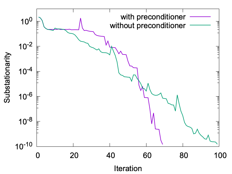
(a) PLAM for He, $\beta=15$

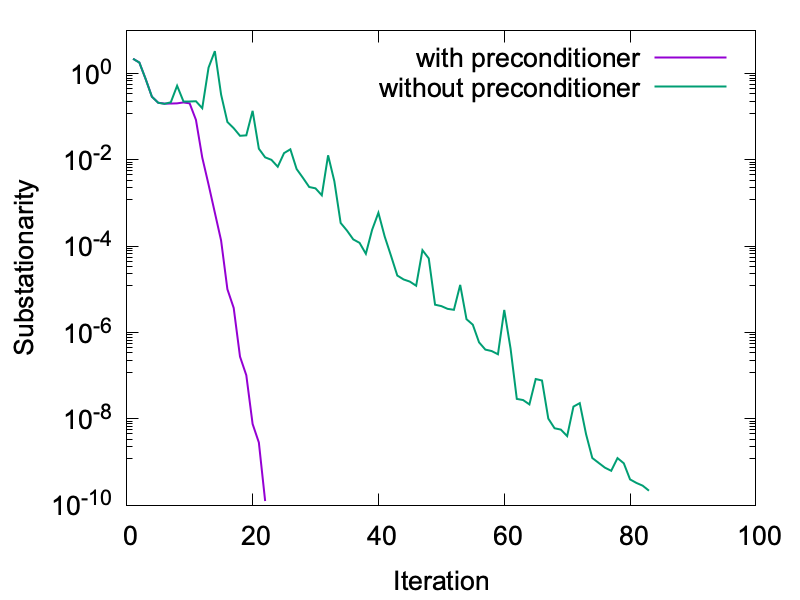
(b) PCAL for He, $\beta=1$

Figure 2: The performance of the preconditioner (28) for a helium (He) atom example with $n=1606,p=1$.

4 Implementation Details

In this section, we introduce the implementation details of the framework (Fig. 1) in solving the ground state. The quantum systems examined in this paper are introduced. In addition, several numerical issues in the simulations are discussed. In view of Fig. 2, we observe that PCAL behaves more efficient and robust than PLAM, and thus we focus on PCAL in the following tests.

All the simulations are performed on a workstation with two Intel(R) Xeon(R) Processors Silver 4110 (at 2.10GHz$\times 8$, 12M Cache) and 384GB of RAM, and the total number of cores is 16. The software is the C++ library AFEABIC [3] under Ubuntu 18.10.

4.1 Testing problems

A number of atom and molecules are simulated to illustrate the effectiveness and high scalability of the presented algorithm. It is noted that in practical simulations, $p$ is regarded as the number of orbitals and each orbital is occupied by two electrons. The scale of testing systems, i.e., $p$, is ranging from 1 to 1152. In the formulation of problem (2), the exchange-correlation potential $V_{\mathrm{xc}}$ and exchange-correlation potential energy $\epsilon_{\mathrm{xc}}$ per particle are obtained from the package Libxc [25]. The model equations for the various numerical examples are only different in the external potential term $V_{\mathrm{ext}}$ and precisely in the charge numbers and positions of the nuclei. The charge of a certain nucleus used in numerical experiments is listed in Table 1. The nuclei positions for small molecules are obtained from the calculated geometry part in CCCBDB [16] and for carbon nanotubes are from [10]. In summary, the following electronic structures He ($1$), LiH (2), CH₄ (5), H₂O (5), BF₃ (16), C₆H₆ (21), C₁₂H₁₀N₂ (48), C₆₀ (180), and carbon nanotubes C₉₆ (288), C₁₉₂ (576) and C₃₈₄ (1152) are tested, where the number in the bracket stands for the number of orbitals $p$ in the associated system.

Table 1: Charge number $Z_{j}$ of the nucleus.

	H	He	Li	B	C	N	O	F
$Z_{j}$	1	2	3	5	6	7	8	9

In practice, we evaluate the values for substationarity, feasibility violation and the total energy of each example during the simulations. Specifically, $kkt=\left\|H(X)X-BX\Lambda\right\|_{\mathrm{F}}$, $fea=\left\|X^{\top}BX-I\right\|_{\mathrm{F}}$, and the total energy $E_{\mathrm{KS}}$ is computed from (6). When the summation of $kkt$ and $fea$ is small enough, i.e., the following stopping criterion

$$\frac{kkt+fea}{kkt_{0}}<tol$$

is satisfied, we terminate the algorithm. Here, $kkt_{0}$ is the initial substationarity and $tol$ denotes the tolerance and is chosen to be $1.0\times 10^{-8}$ in our simulations.

4.2 Pre-processing and discretization: mesh and initial guess generation

Once we determine the computational domain, a space discretization is generated for the ground state calculation. To resolve the singularities in the external potential term, a non-uniform mesh for the partition of the computational domain is introduced to obtain high accuracy with least effort. Specifically, a global mesh size function based on the external potential is adopted to generate the nonuniform mesh [20]. Within the linear finite element framework, to capture the $1/r$ decay in the external potential, the mesh size function locally behaves as $r^{6/5}$ for small $r$ can be derived, where $r$ represents the distance to the nucleus. Then we can construct the mesh size function $h(\bm{r})$ at the discretized point $\bm{r}$ as in [20]:

(29) $$h(\bm{r})=\min\left\{\gamma_{1}Z_{1}^{-\frac{2}{5}}r_{1}^{\frac{6}{5}},\cdots,\gamma_{1}Z_{M}^{-\frac{2}{5}}r_{M}^{\frac{6}{5}},\gamma_{2}\right\},$$

where $r_{j}=|\bm{r}-\bm{R}_{j}|$ represents the distance to the $j$-th nucleus, $\gamma_{1}$ controls the resolution of the mesh, and $\gamma_{2}$ is the largest allowed mesh size. Note that (29) implies that the closer to the nucleus, the smaller the mesh size, i.e., the denser the mesh grid, which is as desired. Moreover, the distribution of the mesh grid around the nucleus with larger charge is also denser than that around the nucleus with a smaller charge. This can be verified from Fig. 3 which shows an radial mesh example for the water molecule (H₂O).

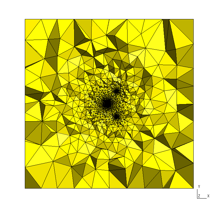
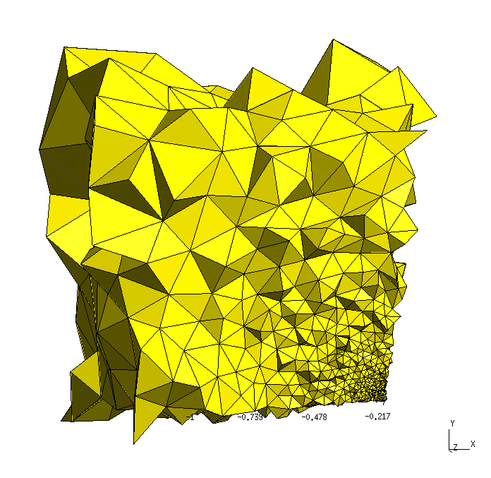
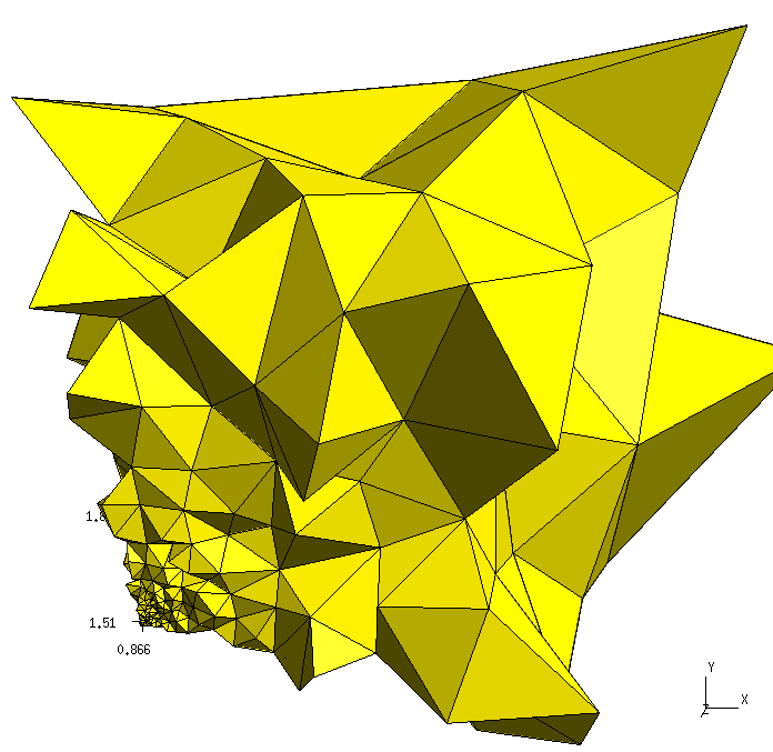
Figure 3: Left: the three dimensional mesh for molecule H₂O using the mesh size function (29) with $\gamma_{1}=0.15,\gamma_{2}=8$. Middle: the mesh around the oxygen nucleus $(-0.217,0,0)$ in X-Y plane $[-1.217,-0.217]\times[0,1]$, on which the element shapes are kept. Right: the mesh around the hydrogen nucleus $(0.866,1.509,0)$ in X-Y plane $[0.866,1.866]\times[1.509,2.509]$. Generated by the software Gmsh v3.0.6 [14].

In the following comparison, we choose a same randomly generated initial guess, $X^{0}\in\mathbb{R}^{n\times p}$ satisfying ${X^{0}}^{\top}B{X^{0}}=I$, for different methods. Given a random matrix $V\in\mathbb{R}^{n\times p}$ from the pseudo-random number generator, $X^{0}$ is generated by the Cholesky-based Gram–Schmidt technique [13], i.e., $V=X^{0}R$, where $R\in\mathbb{R}^{p\times p}$ is an upper triangular matrix. However, it is known that the SCF method may suffer a lot from divergence. For the sake of fairness, we stabilize SCF by improving the random initial guess with the imaginary time propagation (ITP) method [20] only when it diverges. By contrast, the numerical experiments in Section 5 show that our algorithm behaves robust regardless of different initial guesses.

4.3 Post-processing: eigenvalue evaluation in the last step

In view of the presented infeasible methods, it is sufficient to output results such that $X$ satisfies the orthogonality constraint $X^{\top}BX=I$. However, if we want to extract the desired wavefunctions from the eigenvectors of the generalized eigenvalue problem (9) or the other physical quantities based on the eigenvalues, we need to introduce a post-processing. This is due to the fact that $X$ only provides an orthogonal basis of the desired eigenspace rather than the eigenvectors.

This can be implemented by solving a small $p\times p$ eigenvalue problem, $(X^{\top}HX)\tilde{X}=\lambda\tilde{X}$, with the Rayleigh-Ritz procedure to get the eigenvalues $\lambda_{i},i=1,\dots,p$ and updating $X$ as $X=X\tilde{X}$ to get the wavefunctions. Note that this procedure is called only for once in the algorithm and it is of size $p\times p$. Consequently, its computational cost can be ignored compared to solving the optimization problem.

To verify the effectiveness of the post-procedure, we compute the eigenvalues of the Kohn–Sham equation of CH₄ system on the radial mesh with $n=100127,p=5$ for SCF and PCAL. The computational domain for this example is set as $[-20,20]^{3}$, and the results are listed in Table 2. When the post-procedure is imposed, the eigenvalues from PCAL are well ordered and agree with eigenvalues from SCF. Moreover, it verifies that the post-procedure does not affect the energy value. In the practical simulations, the post-procedure step will be imposed as the final step of PCAL.

Table 2: Eigenvalue and energy evaluations for example CH₄.

	$\lambda_{0}$	$\lambda_{1}$	$\lambda_{2}$	$\lambda_{3}$	$\lambda_{4}$	$E_{KS}$
SCF	-9.75599	-0.66451	-0.38832	-0.38830	-0.38825	-40.24109
PCAL + post-processing	-9.75599	-0.66451	-0.38832	-0.38830	-0.38825	-40.24109

4.4 Choices of parameters

There are two major parameters in the algorithm PCAL. In view of Fig. 2, the penalty parameter $\beta=1$ works well for PCAL, and hence $1$ is set as the default value of $\beta$ in PCAL. Next, we investigate the proximal parameter $\eta_{k}$, whose reciprocal is the stepsize for the gradient-descent step in Algorithm 2. As suggested in [12], the Barzilai–Borwein (BB) strategy [4] is an efficient way to produce the stepsize,

$${\eta_{k}^{\mathrm{BB}1}}:=\frac{\left|\left\langle S^{k-1},{Y^{k-1}}\right\rangle\right|}{\left\langle S^{k-1},S^{k-1}\right\rangle},\quad\mbox{or}\quad{\eta_{k}^{\mathrm{BB}2}}:=\frac{{\left\langle Y^{k-1},{Y^{k-1}}\right\rangle}}{\left|\left\langle S^{k-1},Y^{k-1}\right\rangle\right|},$$

where $S^{k}=X^{k}-X^{k-1}$, $Y^{k}=\nabla_{X}{\mathcal{L}_{\beta}}(X^{k},\Lambda^{k})-\nabla_{X}{\mathcal{L}_{\beta}}(X^{k-1},\Lambda^{k-1})$. It has other variations such as the Alternating BB strategy [9],

$$\eta_{k}^{\mathrm{ABB1}}:=\left\{\begin{array}[]{cl}\eta_{k}^{\mathrm{BB}1},&\mbox{for odd}~{}~{}k,\\ \eta_{k}^{\mathrm{BB}2},&\mbox{for even}~{}~{}k,\end{array}\right.\quad\mbox{or}\quad\eta_{k}^{\mathrm{ABB2}}:=\left\{\begin{array}[]{cl}\eta_{k}^{\mathrm{BB}2},&\mbox{for odd}~{}~{}k,\\ \eta_{k}^{\mathrm{BB}1},&\mbox{for even}~{}~{}k.\end{array}\right.$$

We test PCAL with four choices of the parameter $\eta_{k}$ on several testing problems. The number of iterations to achieve convergence is recorded in Table 3. The notation “-” represents that the stopping criterion has not reached after $1000$ iterations. This table reveals that PCAL with $\eta_{k}^{\mathrm{BB2}}$ behaves robust and has the best performance on number of iterations. As a result, we choose $\eta_{k}^{\mathrm{BB2}}$ as our default proximal parameter in the practical simulations.

Table 3: Number of iterations with different proximal parameters.

	He	LiH	CH4	H2O	C6H6
BB1	409	-	-	-	-
BB2	46	54	75	60	144
ABB1	86	90	129	180	291
ABB2	75	74	90	119	256

5 Numerical Examples

In this section, we numerically investigate the performance and parallel efficiency of the algorithm PCAL in all-electron calculations under the presented framework.

We test the classical SCF method and MOptQR for comparisons. MOptQR is a manifold-based optimization method which can be applied to the KSDFT [33]. All these methods are able to fulfill the solving part in the framework described in Fig. 1. They are different in the main iteration: SCF solves a linear eigenvalue problem; PCAL produces a column-wise gradient-descent update; MOptQR searches along the Riemannian antigradient and projects the step onto the manifold by QR factorization. We choose the locally optimized block preconditioned conjugate gradient (LOBPCG) method [18] as the linear eigenvalue solver in SCF. Moreover, a simple mixing scheme is adopted for SCF, namely, $\rho^{(k+1)}=\alpha\tilde{\rho}^{(k+1)}+(1-\alpha)\rho^{(k)}$ where $\tilde{\rho}^{(k+1)}$ is the electron density obtained from solving the $k$-th step eigenvalue problem and $\alpha$ is the mixing parameter. In both SCF method and MOptQR, the orthogonalization process is implemented by the Cholesky-based Gram-Schmidt technique [13], which is shown to be more efficient than commonly-used Gram-Schmidt procedures.

In the serial setting, the leading order of computational costs is $\mathcal{O}(np^{2})$ among these methods. The reason is that BLAS3 operations, such as $X^{\top}(BX)$, dominate the computing. While the function evaluation does not have a crucial impact on the cost due to the sparsity of discretized Hamiltonian $H$ and mass matrix $B$. In the parallel setting, the total computation cost is divided into parallel and non-parallel parts. The above-mentioned leading cost $\mathcal{O}(np^{2})$ (BLAS3) belongs to the parallel part. However, the orthogonalization process in SCF and MOptQR whose complexity is $\mathcal{O}(p^{3})$ cannot be efficiently parallelized. When $p$ is large, this cost is unaffordable in all-electron calculations. Conversely, PCAL is orthogonalization-free and completely consists of BLAS3 operations, and thus benefits a lot from parallel computing. These claims can be verified in the following experiments.

5.1 Ground state calculations

In this subsection, we test PCAL with SCF and MOptQR in all electron calculations of a list of atom and molecules under serial setting. For all the systems, the computational domain is set to be $[-20,20]^{3}$. The mesh size function (29) is applied to generate the nonuniform mesh for each example. Note that the parameters in (29) are chosen as $\gamma_{1}=0.15,\gamma_{2}=8$ for C₆H₆ and C₁₂H₁₀N₂, and $\gamma_{1}=0.125,\gamma_{2}=8$ for the others. The preconditioner (28) is used in all the methods. For the system C₁₂H₁₀N₂, the initial guess is generated by ITP (see Section 4.2), and we choose the mixing parameter $\alpha=0.15$ for SCF to make it converge. For the other systems, we choose a random initial guess and the mixing parameter $\alpha=0.3$.

The detailed numerical results are listed in Table 4, Fig. 4 and Fig. 5. We observe from Table 4 that: 1) the total energy $E_{\mathrm{KS}}$ obtained by PCAL agrees with SCF and MOptQR; 2) PCAL behaves more efficient than SCF and MOptQR in terms of the running time “CPU(s)”; 3) the number of iterations “$N_{\mathrm{iter}}$” in PCAL is less than MOptQR. Note that the iteration numbers of SCF are always the smallest but conversely the CPU time. This is due to that the inner iterations, i.e., solving the linear eigenvalue problem, are required in each SCF iteration. The efficiency of PCAL can be also observed in Fig. 4 for the example C₆H₆, from which we find that PCAL takes the least CPU time to converge at a given accuracy. In addition, the convergence results for PCAL are demonstrated in Fig. 5. The first column displays the isosurface of the electron density, the last three columns present the convergence history of energy, substationarity and feasibility violation, respectively. We observe that the feasibility violation of PCAL gradually decreases until it converges. Note that the post-processing is not shown in this figure. In the He example, the feasibility violation is close to the machine accuracy since the normalization procedure is equivalent to the orthogonalization procedure in the case of $p=1$.

Table 4: The results in Kohn–Sham total energy minimization

Solver	$E_{\mathrm{KS}}$	$kkt$	$N_{\mathrm{iter}}$	$fea$	CPU(s)	$E_{\mathrm{KS}}$	$kkt$	$N_{\mathrm{iter}}$	$fea$	CPU(s)
	He, $n=34481,p=1$					LiH, $n=63725,p=2$
SCF	-2.86809	9.58-9	36	2.88-15	127	-7.98190	2.15-7	39	2.09-14	617
MOptQR	-2.86808	3.56-8	36	3.55-15	82	-7.98190	1.36-7	70	2.70-15	317
PCAL	-2.86808	5.99-9	46	1.62-15	99	-7.98190	1.25-7	54	2.24-15	264
	CH4, $n=141189,p=5$					H2O, $n=149616,p=5$
SCF	-40.23775	4.83-7	39	6.09-14	3788	-75.83672	1.07-7	44	3.64-14	4246
MOptQR	-40.23775	1.24-7	93	2.67-14	1721	-75.83672	1.48-7	74	2.45-14	1413
PCAL	-40.23775	5.66-6	75	1.59-14	1283	-75.83672	1.33-7	60	4.82-14	1219
	C6H6, $n=241939,p=21$					C12H10N2, $n=522149,p=48$
SCF	-231.05824	5.11-7	41	1.73-13	43901	-571.60648	2.57-8	94	1.64-13	379482
MOptQR	-231.05824	3.60-7	269	5.14-14	21238	-571.60648	7.30-8	501	1.63-13	225856
PCAL	-231.05824	3.71-7	144	7.35-14	11013	-571.60648	5.37-8	148	2.29-13	89116

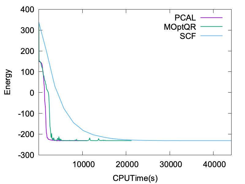
(a) Energy value

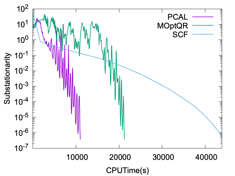
(b) Substationarity

Figure 4: A comparison with different solvers for example C₆H₆.

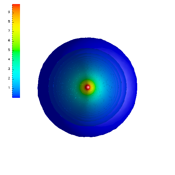
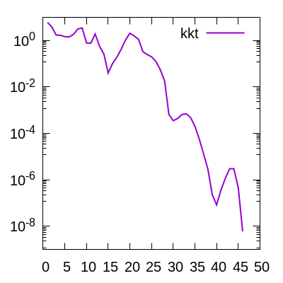
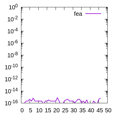
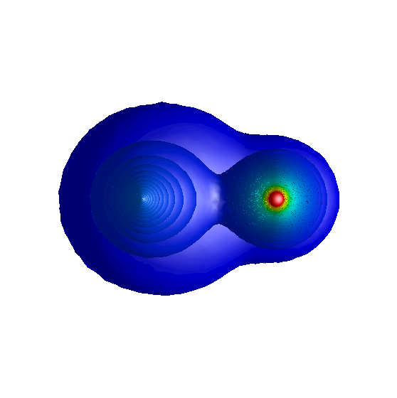
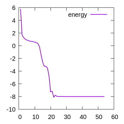
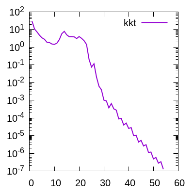
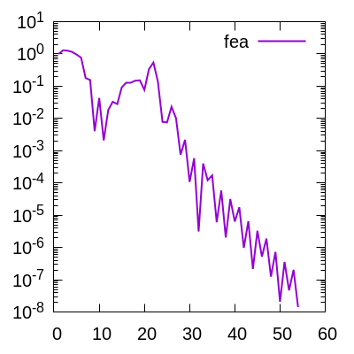
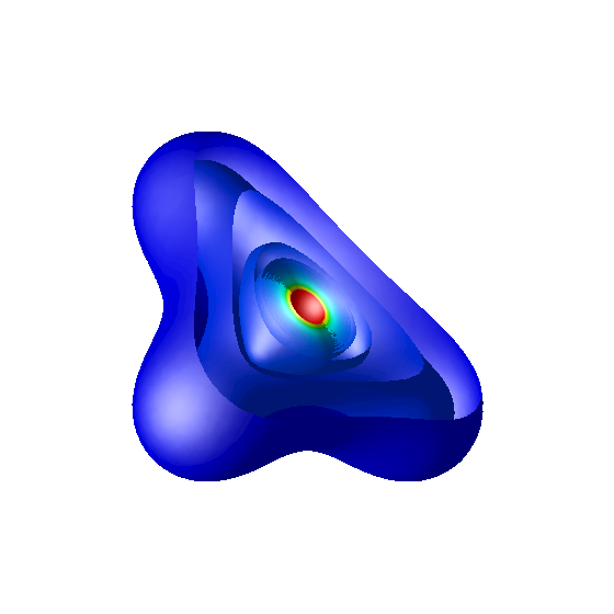
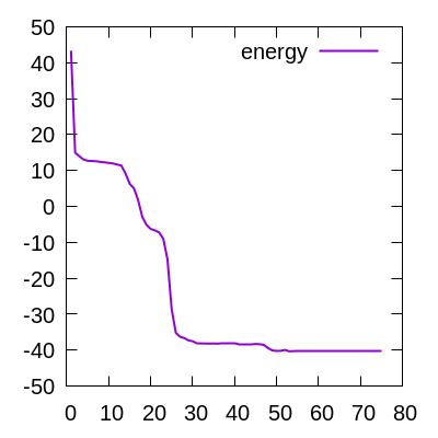
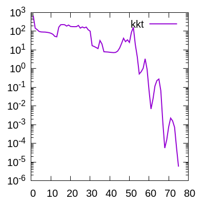
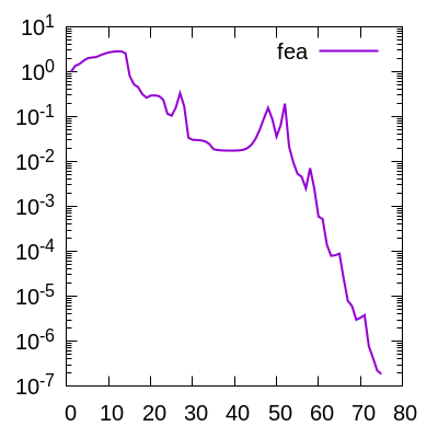
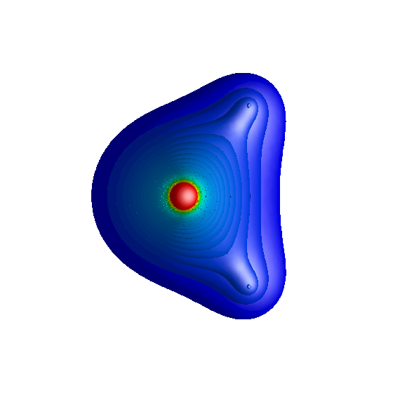
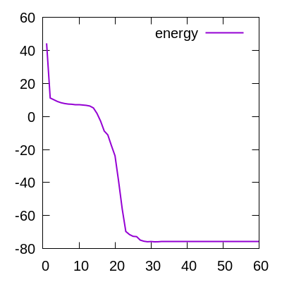
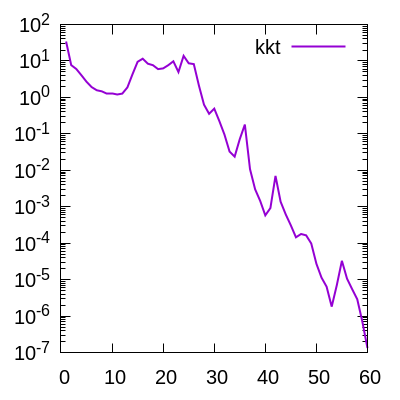
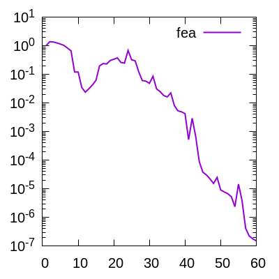
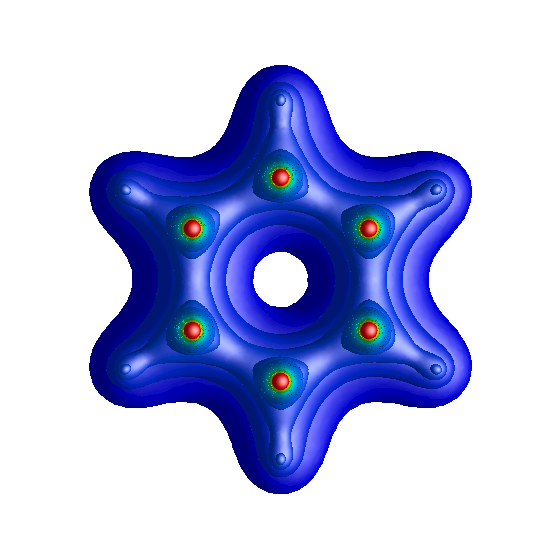
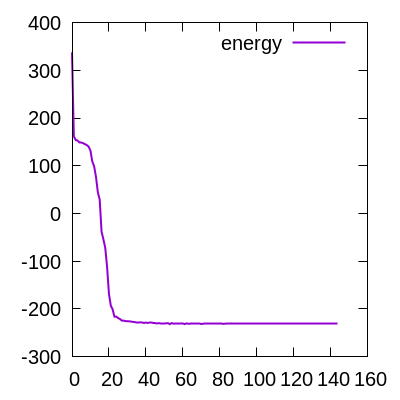
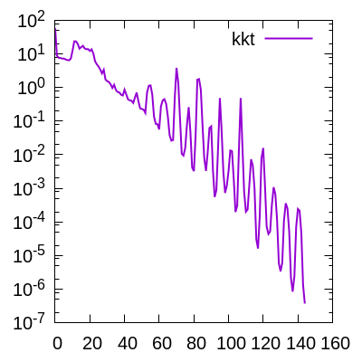
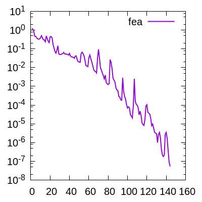
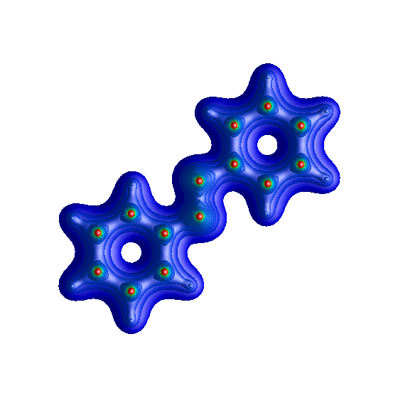
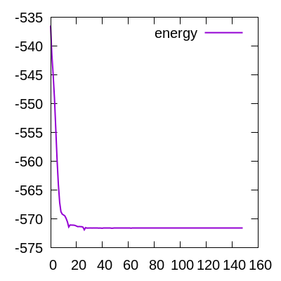
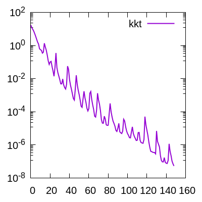
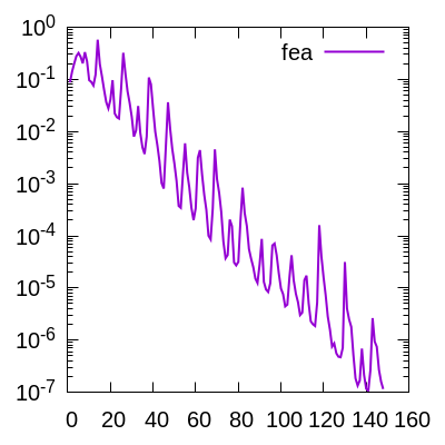
Figure 5: Convergence history of PCAL for He, LiH, CH₄, H₂O, C₆H₆, C₁₂H₁₀N₂ (from top to bottom). The left column displays the isosurface of each molecule. $x$-axis for the right 3 columns stands for the iteration step.

5.2 Scalability

In this subsection, we investigate the parallel efficiency of PCAL. We first test all the algorithms on a single core and record the computational proportions of parallel and non-parallel part in the total cost. We fix $n$ to be around $100000$ and choose different $p$, namely, the different molecules. By adjusting the parameters in Section 4.2, we control the number of mesh grids $n$ being as close as possible to $100000$. The testing examples are BF₃ (16), C₁₂H₁₀N₂ (48), C₆₀ (180), C₉₆ (288), and C₁₉₂ (576). The numerical results are displayed in Fig. 6. We observe that the parallel part of PCAL will dominate the total cost when $p$ becomes large. It is even higher than $99\%$ When $p\geq 180$. This means that PCAL is suitable for parallel computing, especially when the scale of a system is very large. Meanwhile, it can be found that the non-parallel part of SCF and MOptQR becomes large when $p$ increases. The main reason is the cubic complexity $\mathcal{O}(p^{3})$ of orthogonalization process, which cannot be parallelized.

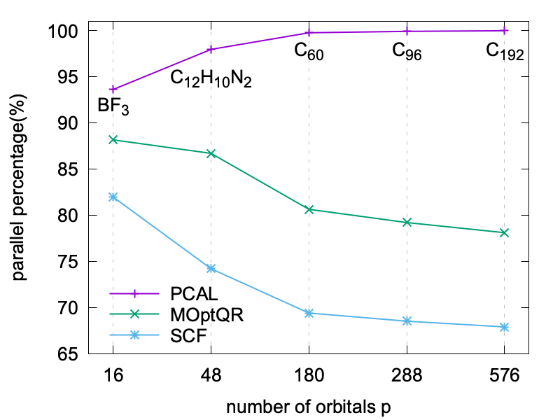
(a) Parallel

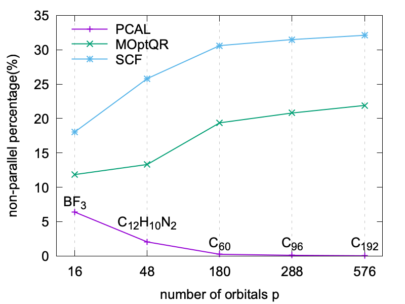
(b) Non-parallel

Figure 6: Parallel proportion versus number of orbitals $p$.

We next examine the scalability of PCAL in the parallel setting. The testing molecule is C₃₈₄ which has $1152$ occupied orbitals. The number of mesh grids $n$ is set to be $380233$. We run the code on different numbers of cores $\{4,8,12,16\}$. The corresponding speedup factor is defined as

$$\text{ speedup-factor }(m)=\frac{\text{ wall-clock time for 4-core run }}{\text{ wall-clock time for a }m\text{-core run }}.$$

The results are presented in Fig. 7, from which we observe that the speedup factor of PCAL is close to the ideal one, and it achieves $3.76$ for $16$ cores. However, MOptQR has the low scalability and its speedup factor increases slowly. Note that the results of SCF are not recorded since the divergent phenomenon is observed. In view of Fig. 6, even if we have the convergent results of SCF, it can be justifiably expected that the speedup factor of SCF will be smaller than that of MOptQR. In summary, the orthogonalization-free algorithm PCAL shows higher scalability and great potential than SCF and MOptQR.

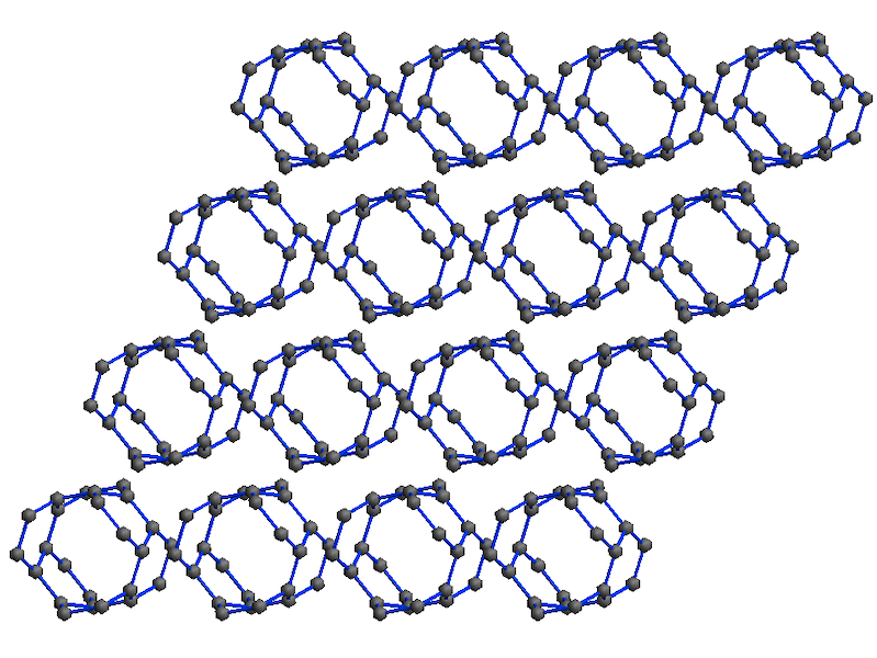
(a) Structure

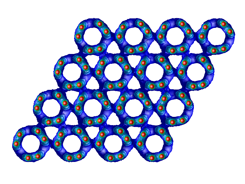
(b) Isosurface

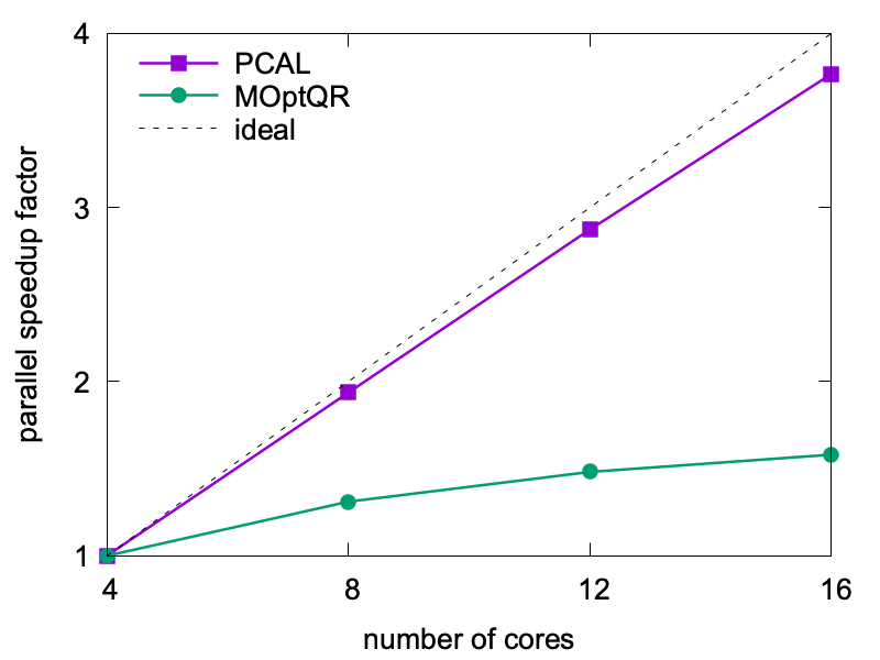
(c) Speedup factor

Figure 7: Example C₃₈₄ with $n=380233$, $p=1152$.

6 Conclusion

Based on the finite element method and PCAL algorithm, a scalable approach is proposed in this paper for the ground state solution of a given quantum system. To resolve the singularity introduced from the all-electron model, a radial mesh is generated according to the structure of the system, then the optimization problem is discretized in the associated finite element space. To avoid the efficiency bottleneck for large scale systems, i.e., the orthogonalization of those orbitals, the original PCAL method is extended and applied in this paper for solving the discretized optimization problem. A novel preconditioner is designed in the extended PCAL method, which generally accelerates the convergence in the simulations.

Comprehensive numerical experiments are implemented for different molecules. The effectiveness of the proposed method is well demonstrated by the comparison among the proposed method, the classical SCF method, and the MOptQR method in serial computing. Meanwhile, the robustness of the proposed method is fully demonstrated by its insensitivity to the initial guess and the algorithm parameters. The feature of the proposed method on improving the efficiency by avoiding the orthogonalization procedure is displayed clearly by the huge reduction of the CPU time in the comparison to the SCF method. More importantly, the excellent scalability of the proposed method is successfully shown in an experiment on a relatively large scale electronic system.

To improve the proposed method, the $h$-adaptive mesh method will be introduced for dynamically adjusting the finite element space according to the obtained numerical solutions. Furthermore, the preconditioner introduced in the PCAL method deserves more investigation in the following study, which has a chance to effectively accelerate the convergence of the numerical method towards the ground state. The improved method will be used for the numerical simulations of the Born-Oppenheimer molecular dynamics, to show the potential on the practical applications. The results will be reported in the forthcoming paper.

References

- [1] P.-A. Absil, R. Mahony, and R. Sepulchre, Optimization algorithms on matrix manifolds, Princeton University Press, 2008, https://doi.org/10.1515/9781400830244.
- [2] R. Ahlrichs, M. Bär, M. Häser, H. Horn, and C. Kölmel, Electronic structure calculations on workstation computers: The program system turbomole, Chem. Phys. Lett., 162 (1989), pp. 165–169, https://doi.org/10.1016/0009-2614(89)85118-8.
- [3] G. Bao, G. Hu, and D. Liu, An -adaptive finite element solver for the calculations of the electronic structures, J. Comput. Phys., 231 (2012), pp. 4967–4979, https://doi.org/10.1016/j.jcp.2012.04.002.
- [4] J. Barzilai and J. M. Borwein, Two-point step size gradient methods, IMA J. Numer. Anal., 8 (1988), pp. 141–148, https://doi.org/10.1093/imanum/8.1.141.
- [5] J. Bolte, S. Sabach, and M. Teboulle, Proximal alternating linearized minimization for nonconvex and nonsmooth problems, Math. Program., 146 (2014), pp. 459–494, https://doi.org/10.1007/s10107-013-0701-9.
- [6] D. R. Bowler and T. Miyazaki, methods in electronic structure calculations, Rep. Prog. Phys., 75 (2012), p. 036503, https://doi.org/10.1088/0034-4885/75/3/036503.
- [7] H. Chen, X. Dai, X. Gong, L. He, and A. Zhou, Adaptive finite element approximations for Kohn–Sham models, Multiscale Model. Sim., 12 (2014), pp. 1828–1869, https://doi.org/10.1137/130916096.
- [8] O. Cohen, L. Kronik, and A. Brandt, Locally refined multigrid solution of the all-electron Kohn–Sham equation, J. Chem. Theory Comput., 9 (2013), pp. 4744–4760, https://doi.org/10.1021/ct400479u.
- [9] Y.-H. Dai and R. Fletcher, Projected Barzilai-Borwein methods for large-scale box-constrained quadratic programming, Numer. Math., 100 (2005), pp. 21–47, https://doi.org/10.1007/s00211-004-0569-y.
- [10] J. T. Frey and D. J. Doren, TubeGen 3.4 web-interface, (2011), http://turin.nss.udel.edu/research/tubegenonline.html (accessed 2019-11-01).
- [11] B. Gao, X. Liu, X. Chen, and Y.-x. Yuan, A new first-order algorithmic framework for optimization problems with orthogonality constraints, SIAM J. Optim., 28 (2018), pp. 302–332, https://doi.org/10.1137/16M1098759.
- [12] B. Gao, X. Liu, and Y.-x. Yuan, Parallelizable algorithms for optimization problems with orthogonality constraints, SIAM J. Sci. Comput., 41 (2019), pp. A1949–A1983, https://doi.org/10.1137/18M1221679.
- [13] L. Genovese, A. Neelov, S. Goedecker, T. Deutsch, S. A. Ghasemi, A. Willand, D. Caliste, O. Zilberberg, M. Rayson, A. Bergman, et al., Daubechies wavelets as a basis set for density functional pseudopotential calculations, J. Chem. Phys., 129 (2008), p. 014109, https://doi.org/10.1063/1.2949547.
- [14] C. Geuzaine and J.-F. Remacle, Gmsh: A 3-D finite element mesh generator with built-in pre-and post-processing facilities, Int. J. Numer. Meth. Eng., 79 (2009), pp. 1309–1331, https://doi.org/10.1002/nme.2579.
- [15] W. Huang and R. D. Russell, Adaptive moving mesh methods, vol. 174, Springer Science & Business Media, 2010, https://doi.org/10.1007/978-1-4419-7916-2.
- [16] R. D. J. III, NIST Computational Chemistry Comparison and Benchmark Database, (2006), http://cccbdb.nist.gov/ (accessed 2019-09-10).
- [17] G. P. Kerker, Efficient iteration scheme for self-consistent pseudopotential calculations, Phys. Rev. B, 23 (1981), p. 3082, https://doi.org/10.1103/PhysRevB.23.3082.
- [18] A. V. Knyazev, Toward the optimal preconditioned eigensolver: Locally optimal block preconditioned conjugate gradient method, SIAM J. Sci. Comput., 23 (2001), pp. 517–541, https://doi.org/10.1137/S1064827500366124.
- [19] W. Kohn and L. J. Sham, Self-consistent equations including exchange and correlation effects, Phys. Rev., 140 (1965), p. A1133, https://doi.org/10.1103/PhysRev.140.A1133.
- [20] Y. Kuang and G. Hu, On stabilizing and accelerating SCF using ITP in solving Kohn–Sham equation, Commun. Comput. Phys., accepted.
- [21] P. R. Levashov, G. V. Sin’ko, N. A. Smirnov, D. V. Minakov, O. P. Shemyakin, and K. V. Khishchenko, Pseudopotential and full-electron DFT calculations of thermodynamic properties of electrons in metals and semiempirical equations of state, J. Phys. Condens. Matter, 22 (2010), p. 505501, https://doi.org/10.1088/0953-8984/22/50/505501.
- [22] L. Lin, J. Lu, and L. Ying, Numerical methods for Kohn–Sham density functional theory, Acta Numer., 28 (2019), pp. 405–539, https://doi.org/10.1017/S0962492919000047.
- [23] X. Liu, X. Wang, Z. Wen, and Y. Yuan, On the convergence of the self-consistent field iteration in Kohn–Sham density functional theory, SIAM J. Matrix Anal. Appl., 35 (2014), pp. 546–558, https://doi.org/10.1137/130911032.
- [24] X. Liu, Z. Wen, X. Wang, M. Ulbrich, and Y. Yuan, On the analysis of the discretized Kohn–Sham density functional theory, SIAM J. Numer. Anal., 53 (2015), pp. 1758–1785, https://doi.org/10.1137/140957962.
- [25] M. A. L. Marques, M. J. T. Oliveira, and T. Burnus, Libxc: A library of exchange and correlation functionals for density functional theory, Comput. Phys. Commun., 183 (2012), pp. 2272–2281, https://doi.org/10.1016/j.cpc.2012.05.007.
- [26] J. Nocedal and S. J. Wright, Numerical optimization, Springer Science & Business Media, 2006, https://doi.org/10.1007/978-0-387-40065-5.
- [27] M. C. Payne, M. P. Teter, D. C. Allan, T. Arias, and a. J. Joannopoulos, Iterative minimization techniques for ab initio total-energy calculations: molecular dynamics and conjugate gradients, Rev. Mod. Phys., 64 (1992), p. 1045, https://doi.org/10.1103/RevModPhys.64.1045.
- [28] W. E. Pickett, Pseudopotential methods in condensed matter applications, Comput. Phys. Rep., 9 (1989), pp. 115–197, https://doi.org/10.1016/0167-7977(89)90002-6.
- [29] P. Suryanarayana, V. Gavini, T. Blesgen, K. Bhattacharya, and M. Ortiz, Non-periodic finite-element formulation of Kohn–Sham density functional theory, J. Mech. Phys. Solids, 58 (2010), pp. 256–280, https://doi.org/10.1016/j.jmps.2009.10.002.
- [30] E. Tsuchida and M. Tsukada, Adaptive finite-element method for electronic-structure calculations, Phys. Rev. B, 54 (1996), p. 7602, https://doi.org/10.1103/PhysRevB.54.7602.
- [31] H. Y. Xiao, X. D. Jiang, G. Duan, F. Gao, X. T. Zu, and W. J. Weber, First-principles calculations of pressure-induced phase transformation in AlN and GaN, Comput. Mater. Sci., 48 (2010), pp. 768–772, https://doi.org/10.1016/j.commatsci.2010.03.028.
- [32] C. Yang, J. C. Meza, and L.-W. Wang, A trust region direct constrained minimization algorithm for the Kohn–Sham equation, SIAM J. Sci. Comput., 29 (2007), pp. 1854–1875, https://doi.org/10.1137/060661442.
- [33] X. Zhang, J. Zhu, Z. Wen, and A. Zhou, Gradient type optimization methods for electronic structure calculations, SIAM J. Sci. Comput., 36 (2014), pp. C265–C289, https://doi.org/10.1137/130932934.