Abstract

This work is to popularize the method of computing the distribution of the excursion times for a Gaussian process that involves extended and multivariate Rice’s formula. The approach was used in numerical implementations of the high-dimensional integration routine and in earlier work it was shown that the computations are more effective and thus more precise than those based on Rice expansions.

The joint distribution of successive excursion times is clearly related to the distribution of the number of level crossings, a problem that can be attacked via the Rice series expansion, based on the moments of the number of crossings. Another point of attack is the “Independent Interval Approximation” (IIA) intensively studied for the persistency of physical systems. It treats the lengths of successive crossing intervals as statistically independent. Under IIA, a renewal type argument leads to an expression that provides the approximate interval distribution via its Laplace transform.

However, the independence is not valid in most typical situations. Even if it leads to acceptable results for the persistency exponent of the long excursion time distribution or some classes of processes, rigorous assessment of the approximation error is not readily available. Moreover, we show that the IIA approach cannot deliver properly defined probability distributions and thus the method is limited only to persistence studies.

The ocean science community favours a third approach, in which a class of parametric marginal distributions, either fitted to excursion data or derived from a narrow band approximation, is extended by a copula technique to bivariate and higher order distributions.

This paper presents an alternative approach that is both more general, more accurate and relatively unknown. It is based on exact expressions for the probability density for one and for two successive excursion lengths. The numerical routine RIND computes the densities using recent advances in scientific computing and is easily accessible for a general covariance function, via simple Matlab interface.

The result solves the problem of two step excursion dependence for a general stationary differentiable Gaussian process, both in theoretical sense and in practical numerical sense. The work offers also some analytical results that explain the effectiveness of the implemented method.

ASM Classification: 60G15, 60G10, 58J65, 60G55, 62P35, 65C50, 65D30
Keywords : diffusion, Generalized Rice formula, persistency exponent,

1 Introduction

1.1 The problem and some of its early history

One of the central problems in Rice’s second article on random noise, (Rice,, 1945), is the statistical characterization of the zeros of a stationary Gaussian process. Rice’s formula for the expected number of zeros, and more generally, of non-zero level crossings, is a first step, but Rice also presents the in- and exclusion series, the “Rice series”, for the distribution of the time between two successive mean level crossings.

The distribution of the number of zero crossings is naturally connected to the distribution of the time series of successive lengths of excursions above and below zero. Both lines of approach were followed during the decades following Rice’s article.

Longuet-Higgins, (1962, 1963) improved considerably on the original Rice series for the number of crossings and derived a rapidly converging moment series for the probability density of zero crossing intervals. He also compared approximations based on the initial terms in the series, with experimental results, (Favreau et al.,, 1956), and with earlier alternative series, suggested by McFadden, (1956, 1958). Early experiments with the series of zero crossing intervals were also performed by Blötekjær, (1958).

The studies by McFadden, (1958) and Rainal, (1962), with more details in (Rainal,, 1963), are of particular interest for the present article, since they contain systematic theoretical as well as experimental studies of the dependence between successive crossing intervals. Three approximation candidates were studied, independence, “quasi”-independence, which i.a. assumes that the sum of two successive intervals is independent of the next one, and Markov dependence. The first two cases were analysed by renewal type arguments and Laplace transforms, (Cox,, 1962; Sire,, 2008), and numerical solutions were compared to experiments. The Markov assumption, first suggested by McFadden, (1957), was tested by variance and correlation parameters against experiment. All three assumptions were rejected for general Gaussian processes.

The tradition with experimental testing of the dependence assumptions, including the Markov assumption, was continued by Mimaki, (1973) and co-workers, (Mimaki et al.,, 1981, 1984, 1985). Munakata, (1997) listed solved and unsolved crossing problems, focusing on experimental evidence and practical application of the available traditional methods to noise in signals.

On the theoretical side, Cramér and Leadbetter, (1967) derived formulas for crossing moments of arbitrary order under minimal assumptions for Gaussian processes, and Zähle, (1984) gave a generalized Rice’s formula for non-Gaussian processes. Lindgren, (1972) introduced a regression technique, (Slepian,, 1963), for the excursion length in a differentiable Gaussian process, a technique that formed a first step towards the numerical algorithms that will be used in this paper.

1.2 Renewed interest and new exact tools

During the years around 1990 the interest in crossing interval distributions and their tail behaviour increased in material science, optics, statistical physics, and other areas, (Brainina,, 2013). In this work, the emphasis was on the tail distribution of the crossing interval often referred to as persistency and, in particular, on its the rate of the convergence to zero, as expressed by the persistency exponent. The “independent interval assumption” (IIA) was applied both to Gaussian processes and to other process models, and compared to experiments. Sire, (2008) describes the renewal and Laplace transform arguments, and gives many references from the physics literature. The diffusion processes and their persistency exponent was analyzed in (Majumdar et al.,, 1996). In the following development, involving experiments, simulations, and theoretical analysis of diffusion phenomena has led to deepened insight into the asymptotic properties of crossing distribution for a range of stochastic processes, as conveniently surveyed in (Bray et al.,, 2013), and with recent advances given in (Poplavskyi and Schehr,, 2018), where an important explicit form of the persistency coefficient for the diffusion of order 2 has been obtained by rather deep combination across different developments in theoretical physics.

In other than physics areas of research, one should notably point to the ocean science and engineering literature. There in the studies of metaocean, the time on successive crossing periods has been studied for the particular spectra occurring in different sea states (Wist et al.,, 2004). Parametric spectra has been proposed tying the natural condition at geographical location and at the sea state at given time and time crossing distribution has been elaborated in many examples (Ochi,, 1998).

During the same years, new tools were developed in applied probability and in scientific computing. Durbin, (1985) gave the exact expression for the first passage density of a non-differentiable Gaussian process to a general level. The result was generalized to smooth processes by Rychlik, 1987a , who also expanded the formula to give the exact probability density of excursion intervals for a differentiable Gaussian process, (Rychlik,, 1990). The exact formula gave the marginal distribution only, but Rychlik, 1987b also used the regression technique, described in (Lindgren and Rychlik,, 1991), to derive an almost correct density for the joint distribution of two successive intervals.

Podgórski et al., (2000) presented the exact formula for the joint density of two or more successive crossing intervals. The formulas, to be described in Section 3, involve the conditional expectations of the derivatives at crossings and the indicator functions that the process stays above or below the level in the intervals between crossings. No analytic expressions for these expectations are known, but they are readily computable by the high-dimensional integration methods that have been made possible by advances in scientific computing.

By proper use of numerical linear algebra and numerical integration techniques Genz, (1992) and Rychlik, 1992a almost simultaneously developed practically useful routines for computation of high-dimensional normal integrals. Genz’s routines were expanded to very high dimensions, (Genz and Kwong,, 2000), while Podgórski et al., (2000), amended Rychlik’s routine to include conditioning on level crossings and derivatives. The routine, called RIND, was included in the Matlab toolbox WAFO; see (Brodtkorb et al.,, 2000) and (WAFO-group,, 2017). Brodtkorb, (2006) combined all the described ideas into a powerful computational tool, adding new tests to control accuracy, and embedding it in user-friendly code for use on Gaussian process crossing problems.

2 A background on interval dependence and the IIA

2.1 A smooth process and its clipped version

2.1.1 Distribution relations

We consider a smooth process $X(t),-\infty<t<\infty$, and the time instants of $u$-level crossings, $S_{i}$, leading to two sequences of interlaced intervals of lengths $T_{i}^{+}$, $i=\pm 1,\pm 2,\dots$, for the excursions above $u$-level and $T_{i}^{-}$, $i=\pm 1,\pm 2,\dots$, for the analogous excursions below $u$. We label the interval that contains the origin $T_{0}^{\pm}=A+B$; it may be an excursion above or below $u$. Figure 1 explains the principle for indexing. The variable $\delta$ is introduced to keep track of excursions above, $\delta=1$, or below $u$, $\delta=-1$. The process $D_{c}(t)=+1(-1)$ when $X(t)>u(<u)$ is called the clipped version of the $X$-process at level $u$. The clipped process is a special case of a switch process that switches between states $+1$ and $-1$ at random times points.

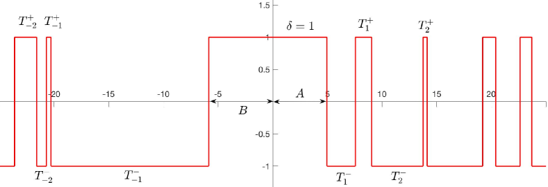
Figure 1: A clipped process $D_{c}$ with the interval $T_{0}^{\pm}$ split in backward and forward delays $B$ and $A$, respectively. The case of the origin state $\delta=1$.

If the smooth process $X(t)$ is stationary, i.e. its distribution is unchanged after a shift of time, its clipped version $D_{c}(t)$ is also stationary. The point process of $u$-level crossings $\{S_{i}\}$, is a stationary point process, the joint distribution of the number of points in disjoint time intervals only depends on the length and relative locations of the time intervals, not on their absolute locations.

We now turn to the distributions of the interval lengths $T_{i}^{+}$ and $T_{i}^{-}$, which are uniquely determined by the distribution of the $X$-process. This needs some care. In Figure 1 we split the interval that contains the origin in two parts, with a forward delay time $A$ to the first crossing on the positive side, and a backward delay time $B$ since the last crossing on the negative side.

We seek the relation between the distribution of $A,B$ and the interval distributions observed in an infinitely long realization of an ergodic process. Denote, for a fixed level $u$, by $f_{T}^{+}(t)$ and $f_{T}^{-}(t)$ the probability densities of the excursions above and below the level, respectively. For a Gaussian process, when $u$ is equal to the mean level, the two densities are equal, $f_{T}(t)=f_{T}^{+}(t)=f_{T}^{-}(t)$ and the clipped process is symmetric with respect to the abscissa. Let $\mu^{+},\mu^{-}$, and $\mu$ denote the mean interval lengths in the asymmetric and symmetric cases.

For a symmetrically clipped process we introduce the following densities: $f_{A,B}(t)$, the joint density of the forward delay $A$ and the backward delay $B$; $f_{A+B}(t)$, the density of the interval that contains the origin; $f_{A}(t)=f_{B}(t)$, the marginal densities of the forward and backward delay times. The simple expressions are

$$f_{A,B}(a,b) =\frac{f_{T}(a+b)}{\mu},$$ (1a)

$$f_{A+B}(t) =\frac{tf_{T}(t)}{\mu},$$ (1b)

$$f_{A}(t)=f_{B}(t) =\frac{\int_{t}^{\infty}f_{T}(s)\,\mathrm{d}s}{\mu},$$ (1c)

with the intuitive interpretation of (1a) that the location of the origin relative to the endpoints of the “center” interval is uniform; see Daley and Vere-Jones, (2008, Exercise 13.3.2). and Appendix A.3. Obviously we can conclude from (1c) that if inter-crossing time and first crossing time have the same distribution, then this distribution is necessarily exponential. The converse is evident.

For the asymmetric case, with $\delta=\pm 1$ indicating the status of the interval that contains the origin, the distribution of $(A,B,\delta)$ is given through

$$\begin{split}\text{\sf P}{(\delta=1)}=\frac{\mu^{+}}{\mu^{-}+\mu^{+}},&~{}\text{\sf P}{(\delta=-1)}=\frac{\mu^{-}}{\mu^{-}+\mu^{+}},\\[3.00003pt] f_{A,B|\delta}(a,b\mid 1)=\frac{f^{+}(a+b)}{\mu^{+}},&~{}f_{A,B|\delta}(a,b\mid-1)=\frac{f^{-}(a+b)}{\mu^{-}},\end{split}$$ (2)

where $f_{A,B|\delta}$ stands for the conditional density.

The discrepancy between the long run interval distributions in a stationary point process and distributions taken from a frozen starting point has been first discussed for telephone calls and solutions have been worked out in the context of Palm measures, renewal processes, horizontal window conditioning, and the Rice formula. The mathematical foundations have been long resolved, see (Palm,, 1943), (Khinchin,, 1955), (Ryll-Nardzewski,, 1961), and (Daley and Vere-Jones,, 2008), as well as in the key renewal theorem.

The clipped process is stationary by its design. However, we observe that for the intervals of its constant values (plus or minus one) that include the origin of the horizontal axis are not distributed the same as the intervals of constant values (excursion intervals) as observed over the entire real line. This can be observed in Figure 2, where the distribution of the excursion intervals including the origin are contrasted with the excursion intervals as collected over the whole line. In fact, as observed in the graphs, the distribution of the in-between intervals over the whole line is closer to the distribution of the distance from the origin to the first crossing rather than the distribution of the entire in-between interval containing the origin. We conclude that statistically speaking the origin of the horizontal line hits larger intervals than those following from the distribution of the excursion times in agreement with the well known inspection paradox.

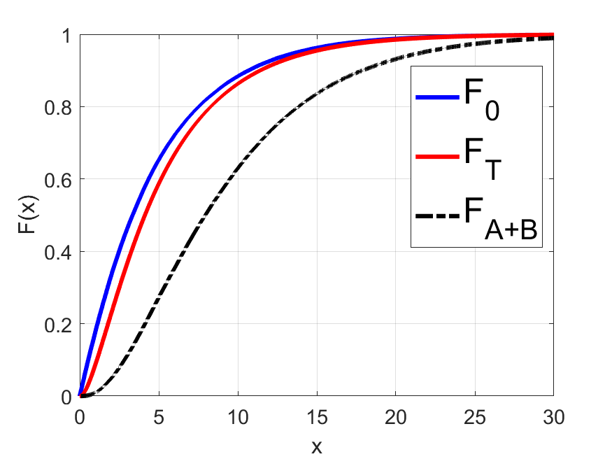
Figure 2: Cumulative distribution functions (cdf) for the distance from the origin to the first crossing (blue), in-between switch times including the origin (black, dash-dotted), and all in-between switch times (red) for a Gaussian switch process LH1, in Table 1.

2.1.2 Covariance function and its Laplace transform

For a smooth stationary process $X(t)$, we define a clipped process at the level $u$ as a process $D_{c}(t)$ that takes value one when $X(t)>u$ and value minus one when $X(t)<u$. It is obvious that $D_{c}$ is also a stationary process and its intervals of constant values contains information about the length of excursions above the level $u$. Therefore properties of the clipped process have been used for analysis of persistence of the underlying process $X(t)$.

It is rather obvious that the covariance of the clipped process can be written as follows

$$R_{u}^{c}(t) =\text{\sf Cov}{(D_{c}(t+s),D_{c}(s))}=\text{\sf P}{(X(t)>u,X(0)>u)}+\text{\sf P}{(X(t)<u,X(0)<u)}$$

$$~{}\hskip 14.22636pt-\text{\sf P}{(X(t)<u,X(0)>u)}-\text{\sf P}{(X(t)>u,X(0)<u)}-\left(1-2F_{X}(u)\right)^{2}$$

$$=4F_{X}(u)\left(\text{\sf P}{(X(t)<u\mid X(0)<u)}-F_{X}(u)\right),$$ (3)

where $F_{X}$ is the cdf of $X(0)$.

Let us additionally assume that the process $X(t)$ is Gaussian with covariance $R_{X}(t)$ and zero mean. In this case, if we denote $\widetilde{u}=u/\sqrt{R_{X}(0)}$ and $\rho_{t}=R_{X}(t)/R_{X}(0)$, then the respective probabilities can be written as

$$\text{\sf P}{(X(t)<u\mid X(0)<u)} =\text{\sf P}(\rho_{t}Z+\sqrt{1-\rho_{t}^{2}}\,Y<\widetilde{u}\mid Z<\widetilde{u})$$

$$=\text{\sf E}{\left({\Phi}\left(\frac{\widetilde{u}-\rho_{t}Z}{\sqrt{1-\rho_{t}^{2}}}\right)\,\Big{|}\>Z<\widetilde{u}\right)},$$

where $Z$ and $Y$ are independent standard normal variables. In the Gaussian case

$$R_{u}^{c}(t) =4\Phi(\widetilde{u})\left(\text{\sf E}{\left({\Phi}\left(\frac{\widetilde{u}-\rho_{t}Z}{\sqrt{1-\rho_{t}^{2}}}\right)\,\Big{|}\,Z<\widetilde{u}\right)}-\Phi(\widetilde{u})\right)$$

$$=4\Phi(\widetilde{u})\left(\frac{1}{\sqrt{2\pi}\Phi(\widetilde{u})}\int_{-\infty}^{\widetilde{u}}e^{-\frac{z^{2}}{2}}{\Phi}\left(\frac{\widetilde{u}-\rho_{t}z}{\sqrt{1-\rho_{t}^{2}}}\right)\,\mathrm{d}z-\Phi(\widetilde{u})\right),$$

where $Z$ is a standard normal random variable.

The formula for the auto-covariance takes a particularly simple explicit form for the symmetric case of level $u=0$, $R_{0}^{c}(t)=\frac{2}{\pi}\arcsin\rho_{t}$. Since the covariance $\rho_{t}$ defines a Gaussian process up to a scaling constant, we see, somewhat surprisingly, that clipping a Gaussian process does not lose any structural information about the original process.

To apply IIA we will link the structure of the clipped process to that of a switch process with independent intervals. The link will be the covariance functions, or rather their Laplace transforms; for the clipped process, $\mathcal{L}R_{u}^{c}(s)=\int_{0}^{\infty}e^{-st}R_{u}^{c}(t)\,\mathrm{d}t$, and for the Gaussian symmetric case,

$$\mathcal{L}\left(\frac{2}{\pi}\arcsin\rho_{t}\right),$$ (4)

that will be matched with the Laplace transform $\mathcal{L}R$ of the stationary covariance $R(t)$ of a switch process with independent intervals.

2.2 A renewal point process and its switch process

2.2.1 A switch process

The clipped process $D_{c}(t)$ is generated from a smooth stationary process $X(t)$ via the point process of $u$-level crossings. That mechanism imposes certain restrictions on its distribution. For example, it is well-known that no non-trivial Gaussian process can have exactly independent mean level crossing intervals, see Palmer, (1956); McFadden, (1958); Longuet-Higgins, (1962).

A start from a general simple stationary point process gives more flexibility for a switch $\pm$ process. To distinguish the construction from the clipping procedure we consider a stationary marked point process $\{S_{i}\}$ on the real line where a sequence of alternating marks $\varepsilon_{i}$ attached to the points indicate if the switch is $-/+$ or $+/-$. The distances between a $-/+$ switch at $S_{i}$ and the following $+/-$ switch is labelled $T_{i}^{+}=S_{i+1}-S_{i}$, while the next switch interval, from $+/-$ to $-/+$, is denoted $T_{i}^{-}$. We denote the switching process by $D_{s}(t)$, and introduce the conditional probabilities

$$P_{\delta}(t) =\text{\sf P}(D_{s}(t)=1\mid D_{s}(0)=\delta),\;\delta=\pm 1.$$

Note that relations (1) and (2) hold for $D_{s}(t)$

2.2.2 A renewal switch process and its covariance function

If all $T_{i}^{+}$ and $T_{i}^{-}$ are independent we have an alternating (delayed) renewal process, and if the distribution of the centre interval is given by (2) then we have a stationary switching process, and it has the “Independent Interval Property”, IIP, (as different from Approximation). Such a process has covariance function $R^{s}(t)=\text{\sf Cov}{(D_{s}(t_{0}),D_{s}(t_{0}+t))}$ of the form

$$R(t) =\frac{2}{\mu^{+}+\mu^{-}}\left(P_{1}(t)\mu^{+}-P_{-1}(t)\mu^{-}+\mu^{+}\frac{\mu^{-}-\mu^{+}}{\mu^{+}+\mu^{-}}\right),$$

The Laplace transform of the covariance is given by the Laplace transforms of the interval distributions, $\Psi_{\pm}(s)=\int_{0}^{\infty}e^{-st}f_{\pm}(t)\,\mathrm{d}t$ and the mean interval lengths, $\mu_{+}$ and $\mu_{-}$,

$$\mathcal{L}R(s) =\frac{4}{s\left(\mu^{+}+\mu^{-}\right)}\left(\frac{\mu_{+}\mu_{-}}{\mu_{+}+\mu_{-}}-\frac{1}{s}\frac{(1-\Psi_{+}(s))(1-\Psi_{-}(s))}{1-\Psi_{-}(s)\Psi_{+}(s)}\right).$$ (5)

In the case when the distributions of $T_{i}^{+}$ and $T_{i}^{-}$ are the same, we obtain the two relations

$$\mathcal{L}R(s) =\frac{1}{s}\left(1-\frac{2}{s\mu}\>\frac{1-\Psi(s)}{1+\Psi(s)}\right),$$ (6)

$$\Psi(s) =\frac{2-s\mu(1-s\,\mathcal{L}R(s))}{2+s\mu(1-s\,\mathcal{L}R(s))}.$$ (7)

The above result is in agreement with formula (215) in Bray et al., (2013).

2.3 The persistence exponent and the IIA

2.3.1 The IIA principle

We can now formally state the fundamentals of the IIA approach.

The IIA principle for symmetric crossing distance: Find the covariance function $R_{c}(t)$ (3) of the clipped process from its distribution and match its Laplace transform to that of a symmetric renewal process (6),

$$\mathcal{L}R_{c}(s) =\mathcal{L}R(s)=\frac{1}{s}\left(1-\frac{2}{s\mu}\>\frac{1-\Psi(s)}{1+\Psi(s)}\right),$$ (8)

and solve for $\Psi(s)$, according to (7). If the clipped process is Gaussian, set $\mathcal{L}R_{c}(s)=\mathcal{L}\left(\frac{2}{\pi}\arcsin\rho_{t}\right)(s)$.

We note that in the symmetric case the inter-switch distribution is a function only of the Laplace transform of the covariance function. For the asymmetric case, (5), there are two distributions, $f_{+}$ and $f_{-}$, to be matched to the covariance function. Thus if we do have the covariances of the switch process, we need one more relation to solve for these distributions. For that different strategies could be taken. For example, one can match two Slepian models for upcrossing and downcrossing with the non-stationary mean of the non-delayed switch process. In the result one could determine both $f_{+}$ and $f_{-}$, see also (Sire,, 2007) and (Sire,, 2008) for the related approach.

When closely examined, the approach is somewhat mathematically inconsistent as it uses the poles of a Laplace transform of a function that is not a probability distribution to approximate the distributional tails of the inter-crossing intervals. This is because the solution $\Phi$ of (8) does not, in general, correspond to a valid probability distribution. In Appendix A.5, we further elaborate on these issues.

Nevertheless, the IIA principle, while not delivering a valid approximation of the distribution, works fairly well in approximating its tail behavior. The latter is best described in the terms of the persistency exponent.

2.3.2 The persistence exponent

The most common meaning of persistence is as the tail of the first-crossing distribution

$$Q_{T} =\text{\sf P}(X(t)\text{ does not change sign between $t=0$ and $t=T$}),$$ (9)

in particular for large $T$. Alternatively, the probability that the process stays above (or below) the level $u$ in the entire interval $[0,T]$.

For Gaussian processes the asymptotic behaviour of the persistence depends only on the covariance function. General results about the asymptotic persistence are scattered and not very precise. The most precise statements about the decay have been formulated for processes with non-negative correlation function, while for oscillating correlation only upper and lower bounds have been obtained.

Non-negative correlation:

(Dembo and Mukherjee,, 2015, Thm. 1.6) give a precise meaning to the “exponential tail” property: If the correlation function $r(t)$ of a stationary centered Gaussian process $X(t)$ is everywhere non-negative, then there exists a non-negative limit

$$b_{r} =-\lim_{T\to\infty}\frac{1}{T}\log\text{\sf P}\left(\inf_{t\in[0,T]}X(t)>0\right).$$ (10)

Feldheim and Feldheim, (2015) comments that $b_{r}$ is necessarily finite, and thus it is meaningful to formulate the persistence tail as

$$Q_{T} =\text{\sf P}\left(\inf_{t\in[0,T]}X(t)>0\right)+\text{\sf P}\left(\sup_{t\in[0,T]}X(t)<0\right)=2e^{-(\theta+o(T))T}=e^{-(\theta+o(T))T},$$ (11)

where $o(T)\to 0$ as $T$ increases without bound (Landau’s little o symbol), with $0\leq\theta=b_{r}$ as the persistence exponent. One should note that since nothing is said about the asymptotics of $o(T)\cdot T$, relation (11) only gives the main order of decay in the sense that for every $\varepsilon>0$, $Q_{T}/\exp(-(\theta\pm\varepsilon)T)\to(0,\infty)$.

Oscillating correlation:

Very little is known about the persistence for oscillating correlation. Antezana et al., (2012) studied the low-frequency white noise process with correlation function $r(t)=\sin(t)/t$ and proved the existence of exponential upper and lower bounds,

$$0<e^{-cT} \leq Q_{T}\leq e^{-CT},\text{ with $c,C>0$}.$$ (12)

Feldheim and Feldheim, (2015) generalized (12) to processes whose spectral measure is bounded away from zero and infinity near the origin. The condition is automatically fulfilled if the process has a spectral density $S(\omega)$ with $m<S(\omega)<M$ for all $\omega\in[-a,a]$ for some finite $a,m,M>0$.

Persistence approximation via IIA:

The IIA attempts to approximate the inter-crossing distance distribution through its Laplace transform and the inverse transform. While it fails to deliver the proper distribution, it still yields decent approximations of the tail behavior. In fact, the inter-crossing distance is often close to an exponential density $f_{T}(t)=\theta e^{-\theta t},t>0$, with Laplace transform $\Psi(s)=\frac{\theta}{\theta+s}$. For the exponential distribution $Q_{T}=e^{-\theta T}$ an approximate value $\theta_{IIA}$ for $\theta$ is minus the largest pole of $\Psi(s)$ in (7), i.e.

$$\theta_{IIA}=-\max\{s;2+s\mu(1-s\,\mathcal{L}R(s))=0\},$$ (13)

(Bray et al.,, 2013, Eqn. (217)) for the Gaussian case:

As noted in Section 2.1.1, exponential inter-crossing distance implies exponential first crossing distance with the same parameter. Thus, the persistence exponent $\theta_{per}$, defined by $\text{\sf P}(X(t)\text{ does not change sign between $t=0$ and $t=T$})\propto e^{-\theta_{per}T}$ for large $T$, can be approximated as $\theta_{per}=\theta_{IIA}$. In Appendix A.5, we present the IIA approximation of the persistency exponent for the diffusion in the dimension two.

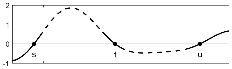
Figure 3: The “triply conditioned” process with successive crossing distances $T_{1}=t-s,T_{2}=u-t$, centred at $t$.

3 Exact non-asymptotic crossing distributions

3.1 The Durbin-Rychlik formula

The root of the exact formula for crossing interval distributions is the “doubly conditioned” process derived by Slepian, (1963), which explicitly describes a process with a level upcrossing at $0$ and downcrossing at $t$; the conditioning is implicit in Rice’s original paper (Rice,, 1945). For our purpose, we illustrate in Figure 3 the “triply conditioned” process with a zero downcrossing at $t=0$ with upcrossings at $s$ and $u$.

We use the following notational conventions from (Podgórski et al.,, 2000): $X_{s,t,u}=(X(s),X(t),X(u))$, $\dot{X}_{s,t,u}=(\dot{X}(s),\dot{X}(t),\dot{X}(u))$, $\dot{X}_{s,t,u}^{+-+}=\dot{X}(s)^{+}\dot{X}(t)^{-}\dot{X}(u)^{+}$, and $X_{s,t}=(u,v)$ means $X(s)=u,X(t)=v$. Moreover, $a\leq X_{s,t}\leq b$ means that for each $u\in(s,t):a\leq X(u)\leq b$, while $\{a\leq X_{s,t}\leq b\}$ also stands for the indicator function of this set, i.e. the function equal to one whenever the condition between the brackets is satisfied and to zero otherwise.

The triple crossing intensity for the configuration in Figure 3 is then equal to a truncated product moment in a conditional normal distribution:

$$\nu^{+-+}(s,t,u) =\int_{z_{1}=0}^{\infty}\int_{z_{0}=-\infty}^{0}\int_{z_{2}=0}^{\infty}z_{1}z_{0}z_{2}\,f_{\dot{X}_{s,t,u},X_{s,t,u}}(z_{1},z_{0},z_{2},0,0,0)\,\mathrm{d}z_{1}\,\mathrm{d}z_{0}\,\mathrm{d}z_{2}$$ (14)

$$=\text{\sf E}[\dot{X}_{s,t,u}^{+-+}\mid X_{s,t,u}=(0,0,0)]\times f_{X_{s,t,u}}(0,0,0).$$ (15)

With $\nu=\int_{0}^{\infty}zf_{\dot{X}(0),X(0)}(z,0)\,\mathrm{d}z$, the zero up/downcrossing intensity, $\nu^{+-+}(s,t,u)/\nu$ is the conditional intensity of upcrossings at $s,u$, given a downcrossing at $t$. To get the distribution of successive crossing intervals one has to qualify the expectation in (15) by requiring that the process stays above $0$ in the entire left interval and below in the entire right interval in Figure 3.

The Rice series approximations achieves the qualifications by restricting the number of extra crossings in the interior of the intervals by higher order moments for the number of crossings. Kan and Robotti, (2017) give recursive formulas how to compute all truncated moments to a very high computational cost.

The exact formula for the distribution of level crossing intervals in Gaussian processes was developed by Durbin, (1985) and Rychlik, 1987a , while Podgórski et al., (2000) extended it to successive intervals, without giving details. Åberg et al., (2008, Thm. 7.1) later presented a complete proof for a very similar case; a short proof is given in Appendix A.4 in the present work.

Since we work with a stationary process, we can take $t=0$, and consider the indicator functions to be included in the conditional expectation in (15), $\{X_{s,0}>0\}$ and $\{X_{0,u}<0\}$. Obviously, $\dot{X}_{s,0,u}^{+-+}=|\dot{X}_{s}\dot{X}_{0}\dot{X}_{u}|$ when both conditions are satisfied.

The exact expression for the probability density of the length of two successive zero crossing intervals is, ($s=-t_{1},u=t_{2}$), (Podgórski et al.,, 2000, Eqn 10),

$$f_{T_{1},T_{2}}(t_{1},t_{2})$$

$$=\nu^{-1}\text{\sf E}[|\dot{X}_{-t_{1}}\dot{X}_{0}\dot{X}_{t_{2}}|\{X_{-t_{1},0}>0>X_{0,t_{2}}\}\mid X_{-t_{1},0,t_{2}}=(0,0,0)]\,f_{X_{-t_{1},0,t_{2}}}(0,0,0).$$ (16)

In the above, the conditional expectation is taken over infinite dimensional set of variables due to the uncountable number of times instants involved in $\{X_{-t_{1},0}>0>X_{0,t_{2}}\}$.

3.2 Evaluation of the expectation involving an uncountable number of instants

Like most, so called, “explicit solutions” to mathematical problems, the expectation in (16) has to be evaluated numerically. The degree of complexity is the same as computing the distribution of the maximum of a smooth non-stationary Gaussian process $X(t)$, $\text{\sf P}(\max_{[0,T]}X(t)\leq x)$, for a finite interval with length $T$; see (Genz and Bretz,, 2009) for available efficient software, and (Azaïs and Genz,, 2013) for an analysis of numerical accuracy.

For our problem, we observe that the variables in the braced indicator in (16) are non-stationary Gaussian, given the condition $X_{-t_{1},0,t_{2}}=(0,0,0)$. The derivatives at the crossing points are not Gaussian but their joint density is proportional to the integrand in (14). If we incorporate the derivatives in the conditioning, the indicator variables are still non-stationary Gaussian.

Due to the strong local dependence for smooth Gaussian processes, the natural way to compute the expectation in (16) is to replace the “infinite-dimensional” indicator $\{X_{-t_{1},0}>0>X_{0,t_{2}}\}$ by a finite-dimensional one. To obtain sufficient accuracy one may have to take a dense grid which can result in an almost singular covariance matrix for the multivariate Gaussian distribution. Brodtkorb, (2004, 2006) discussed several strategies to evaluate nearly singular multinormal expectations. He improved the algorithms proposed by Genz, (1992) and Genz and Kwong, (2000) when the correlation is strong and the number of variables is very large, and, most important, he increased the computing speed and improved memory requirement by utilizing ideas from (Rychlik, 1987c, ; Rychlik, 1992b, ; Podgórski et al.,, 2000). Brodtkorb, (2006) also made extensive studies of the accuracy of the numerical algorithms for a number of realistic applications. The result, the Matlab routine RIND is included in the free package WAFO, (WAFO-group,, 2017), and in the MAGP package by Mercadier, (2006)..

3.3 About RIND

The RIND routine is designed to accurately approximate functionals like

$$\text{\sf E}[|\dot{X}_{-t_{1}}\dot{X}_{0}\dot{X}_{t_{2}}|\{X_{-t_{1},0}>0>X_{0,t_{2}}\}\mid X_{-t_{1},0,t_{2}}=(0,0,0)]f_{X_{-t_{1},0,t_{2}}}(0,0,0),$$ (17)

when $\{X_{-t_{1},0}>0>X_{0,t_{2}}\}$ is replaced by a discrete time restriction, $\{X_{S_{n}^{\prime}}>0>X_{S_{m}^{\prime\prime}}\}$, on equidistant points $s_{k}^{\prime},s_{k}^{\prime\prime}$ in the two intervals:

$$\begin{split}S_{n}^{\prime}&=(-t_{1}<s_{n}^{\prime}<s_{n-1}^{\prime}<\ldots<s_{1}^{\prime}<0),\\ S_{m}^{\prime\prime}&=(0<s_{1}^{\prime\prime}<s_{2}^{\prime\prime}<\ldots<s_{m}^{\prime\prime}<t_{2}).\end{split}$$ (18)

Thus, the problem falls in the category of general multinormal expectations:

$$F(\mbox{\boldmath$a$},\mbox{\boldmath$b$};\mbox{\boldmath$\Sigma$}) =\frac{(2N)^{-N/2}}{\sqrt{|\mbox{\boldmath$\Sigma$}}|}\int_{a_{1}}^{b_{1}}\cdots\int_{a_{N}}^{b_{N}}g(\mbox{\boldmath$x$})\exp\left\{\frac{-\mbox{\boldmath$x$}^{T}\mbox{\boldmath$\Sigma$}^{-1}\mbox{\boldmath$x$}}{2}\right\}\,\mathrm{d}x_{N}\cdots\mathrm{d}x_{1}.$$ (19)

The paper by Genz, (1992) is the main reference to modern techniques for evaluation of the integral. Its focus is on the case $g(\mbox{\boldmath$x$})=1$, but it gives hints on how to handle a general $g$-function. The work by Brodtkorb, (2006) is focused on the special structure of (17) in order to increase efficiency, while using the basic ideas from (Genz,, 1992) and subsequent work. The additional elements include use of the regression approximation by Rychlik, 1987c , removal of redundant integrals, and Cholesky matrix truncation.

The result, the RIND routine, offers several alternative methods for the computation of the integral, including combinations of the following codes by Brodtkorb (2000 and 2004); more details of the alternatives can be found in the Fortran source file intmodule.f in WAFO.

SADAPT:

A generalization by Brodtkorb (2000) of the routine SADMVN in (Genz,, 1992) to make it work not just for the multivariate normal integral.

KRBVRC:

An update by Brodtkorb (2000) of the module KRBVRCMOD by Genz (1998).

KROBOV:

An update by Brodtkorb (2000) of the module KROBOVMOD by Genz (1998).

RCRUDE:

An update by Brodtkorb (2000) of the module RCRUDEMOD by Genz (1998), improving randomized integration.

SOBNIED:

A routine by Brodkorb (2004), improving KRBVRC by using random selection of points as in (Hong and Hickernell,, 2003).

DKBVRC:

An update by Brodtkorb (2004) of a routine with the same name by Genz (2003).

3.4 Calling RIND

The RIND function is a Matlab interface to a set of algorithms, originally written in Fortran and C++, that execute one, or a combination, of the options, SADAPT – DKBVRC. The function takes as input means and covariances of three groups of normal variables. One groups consists of variables to condition on, Xc = xc, like $X_{-t_{1},0,t_{2}}=(0,0,0)$ in (17). The second group, Xd, are the derivatives at crossings, like $\dot{X}_{-t_{1}},\dot{X}_{0},\dot{X}_{t_{2}}$, and the third group Xt contains the variables that have to satisfy an interval condition, xlo $\sansmath{\leq}$ Xt $\sansmath{\leq}$ xup. Such constraints may also be imposed on the derivatives.

The call to RIND has the following input/output structure, extracted from help RIND:

[E,err,terr,exTime,options] = rind(S,m,Blo,Bup,indI,xc,Nt,options);
         E = expectation/density, according to (4)
       err = estimated sampling error
      terr = estimated truncation error.
    exTime = execution time
         S = Covariance matrix of X=[Xt;Xd;Xc]
         m = the expectation of X=[Xt;Xd;Xc]
   Blo,Bup = Lower and upper barriers used to compute the integration bounds
      indI = indices to the different barriers in the indicator function
        xc = values to condition on
        Nt = size of Xt
   options = options structure or named parameters with corresponding values

The options structure is used to select integration method, set error tolerances, alternatively set speed, set seed for Monte Carlo-integration, and many other parameters. As an example of how the speed option affects the result we can take the low-frequency white noise process, illustrated in Figure 6, WN, when integrated by SOBNIED at slowest and fastest speed, speed = 1, and 9, respectively. The joint pdf of two successive zero crossing intervals was calculated at a grid of 120 x 120 = 14 400 points. Execution time was 120 seconds with the slowest option and 45 seconds with the fastest, with an increase in truncation error by a factor $10^{4}$ and in sampling error by a factor $4$ to $10^{2}$. The level curves were virtually identical for levels enclosing up to $90$% of the probability, with only small deviations for the more extremes curves. The plot in Figure 6 was produced in 81 seconds with the KROBOV algorithm, a generally slower method, with speed set to 5.

Remark 1 (RIND and persistence).

The RIND function can be used to compute the persistence for any finite interval $[0,T]$. One just has to let the groups Xc and Xd of conditioning variables and end point derivatives be empty. Setting the lower and upper bounds to $0$ and $\infty$, respectively, the algorithm will give the probability that all the Xt-variables stays above $0$. The covariance matrix S has to be set to the covariance matrix of a sufficiently dense subset of $X(t)$-variables, $X(s_{k});0<s_{k}<T$.

4 RIND and successive level crossing intervals

In this section we give an account of numerical evaluation of crossing distribution properties for Gaussian processes. A complete code using the WAFO toolbox for some of the evaluations is provided in Appendix A.6 to illustrate convenience and simplicity of using the implemented integration routines. It was developed for use on joint crossing intervals in (Lindgren,, 2019).

4.1 Selection of spectra and covariance functions

We study throughout a stationary Gaussian process with mean zero and covariance function $r(t)=\text{\sf Cov}(X(s),X(s+t))$. All processes are smooth with continuously differentiable sample paths and finite number of level crossings in bounded intervals. We refer to (Lindgren,, 2013) for general facts on stationary Gaussian processes, and for differentiability in particular.

We illustrate the RIND method on processes with covariances and spectra of many different types, studied in the literature: (Longuet-Higgins,, 1962; Lindgren,, 1972; Sire,, 2008), (Azaïs and Wschebor,, 2009; Bray et al.,, 2013; Wilson and Hopcraft,, 2017), all listed in Table 1.

Table 1: Un-normalised spectra and covariance functions.

Spectrum Covariance function Source Type: Rational spectrum $(1+\omega^{2})^{-3}$ $e^{-|t|}(1+|t|+t^{2}/3)$ LH1 $(1+\omega^{2})^{-4}$ $e^{-|t|}(1+|t|+6t^{2}/15+|t|^{3}/15)$ LH2 $(1+\omega^{2})^{-5}$ $e^{-|t|}(1+|t|+3t^{2}/7+2|t|^{3}/21+t^{4}/105)$ LH3 ${\omega^{4}}{(1+\omega^{2})^{-5}}$ $e^{-|t|}(1+|t|-t^{2}/3-2|t|^{3}/3+t^{4}/9)$ LH4 $(1+\omega^{2})^{-2}$ $e^{-|t|}(1+|t|)$ LH5 ${\omega^{2}}{(1+\omega^{2})^{-4}}$ $e^{-|t|}(1+|t|-t^{2}/3)$ LH6 ${\omega^{4}}{(1+\omega^{2})^{-4}}$ $e^{-|t|}(1+|t|-2t^{2}+|t|^{3}/3)$ LH7 Type: Shifted Gaussian $\cosh(k\omega)\exp(-\omega^{2}/2)$ $\cos(kt)\exp(-t^{2}/2),k=0,1,2,...$ WHk Type: Noise and sea waves $\bm{1}_{[-1,1]}$ $\sin(t)/t$ WN $(1+\omega^{14})^{-1}$ NA BS Jonswap NA J Type: Diffusion $\displaystyle\operatorname{sech}(\pi\omega)=\frac{1}{\cosh(\pi\omega)},~{}d=2$ $\displaystyle{\operatorname{sech}^{d/2}(t/2)=\frac{1}{\cosh^{d/2}\left(t/2\right)},~{}d\in\mathbb{N}}$ BMSd

Most of the studied processes are, what was called by Longuet-Higgins, (1962), the “regular type”, with covariance function admitting the expansion

$$r(t) =1-\lambda_{2}t^{2}/2+\lambda_{4}t^{4}/4!+o(t^{4+\epsilon}),t\to 0.$$ (20)

In the regular case, the process is twice continuously differentiable and the zero crossing interval pdf is of order $f_{T}(t)\thicksim ct$ for small $t$. The zeros do not cluster.

Processes of the “irregular type” have covariance functions expanded as

$$r(t) =1-\lambda_{2}t^{2}/2+C|t|^{3}/3!+o(|t|^{3}),C\neq 0,$$ (21)

and the crossing density has a universal non-zero limit at the origin,

$$f_{T}(t)\to K\alpha,\text{ where }\alpha=C/6\lambda_{2}.$$ (22)

Longuet-Higgins, (1963, Eqn 47) gives an estimate of the constant $K\approx 1.15597$.

The name convention for the spectra and covariances in Table 1 is as follows. LHk and WHk hint at (Longuet-Higgins,, 1962) and (Wilson and Hopcraft,, 2017). The diffusion spectra BMSd were used in (Bray et al.,, 2013). WN is low-frequency white noise with a Butterworth approximation BS, and the Jonswap spectrum J is an example of an ocean wave spectrum. Note that the spectra and covariance functions are listed in un-normalised form. In the examples they are normalised to $\lambda_{0}=\lambda_{2}=1$ and average zero crossing interval equal to $\pi$. All spectra are of the regular type except LH5–LH7, which are irregular.

The regularity parameter is $\alpha=\lambda_{2}/\sqrt{\lambda_{0}\lambda_{4}}$; $1/\alpha$ is equal to the mean number of local extremes per mean level crossing. In the numerical examples we will relate the $\alpha$-parameter to the correlation coefficient between successive crossing intervals, and to the deviation between the true joint pdf and the pdf under the Independent Interval Assumption, obtained by multiplication of the marginal pdf:s. The Kullback-Leibler distance,

$$KL=-\iint f_{T_{1},T_{2}}(t_{1},t_{2})\log(f_{T_{1}}(t_{1})f_{T_{2}}(t_{2})/f_{T_{1},T_{2}}(t_{1},t_{2}))\,\mathrm{d}t_{1}\mathrm{d}t_{2},$$

is used as a measure of the deviation between full dependence and independence. Note that we use the true marginal pdf  for a Gaussian process when we construct the “independence” pdf, and not the one obtained by the IIA technique. One of the reasons of the difficulty in using the latter is, as explained in Appendix A.5, that the IIA approach typically does not produce a valid probability distribution.

4.2 Computations of the joint distribution of crossing intervals

The joint pdf $f_{T_{1},T_{2}}(t_{1},t_{2})$ for successive mean level crossing intervals are calculated by RIND as described in Section 3.3 via the user interface cov2ttpdf. It takes as input the covariance function in the form of a Matlab symbolic function or the spectrum in the form of a WAFO spectrum structure. Both types of arguments are automatically normalized to $\lambda_{0}=\lambda_{2}=1$. For irregular type processes, the form of the density for small $t_{1},t_{2}$ is not directly resolved by the integration in RIND but the limit (22) can be used to extend the integrated values to $t_{1}=0$ and $t_{2}=0$. The plot for LH7 in Figure LABEL:Fig:nonIIA is constructed in that way. The marginal pdf of the crossing intervals $T_{1}$ and $T_{2}$ are obtained by integrating the bivariate pdf, and a joint pdf under independence is obtained by multiplying the two.

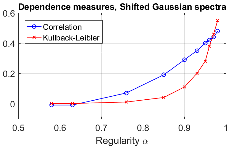
Figure 4: Dependence measures for shifted Gaussian spectra.

We have compared the exact RIND pdf with the IIA-based pdf for all the spectra in Table 1 and we present some typical illustrations. We also give some numerical dependence measures: in Figure 4 for shifted Gaussian spectra and in Table 2 for other examples of spectra.

For each of the spectra, we computed the correlation coefficient between successive half periods, and the Kullback-Leibler distance between the exact pdf and the IIA pdf. Figure 4 shows the smooth relation between the regularity $\alpha$ and the dependence for the shifted Gaussian spectra, WH0-WH9. The theoretical correlations presented in Figure 4 agree with those illustrated in (Wilson and Hopcraft,, 2017, Fig. 8). The spectra in the other group are more diverse and do not exhibit any systematic relation with the regularity measure, (when it exists), as seen in Table 2.

Table 2: Dependence measures for rational, noise, and wave spectrum

model LH1 LH2 LH3 LH4 LH5 LH6 LH7 WN BS J $\alpha$ 0.33 0.45 0.49 0.49 NA 0.50 NA 0.74 0.72 0.70 $\text{\sf Corr}(T_{1},T_{2})$ -0.02 -0.02 -0.02 0.25 0.04 0.19 0.23 -0.01 -0.02 0.44 KL 0.00 0.00 0.00 0.03 0.01 0.02 0.05 0.04 0.01 0.14

We illustrate graphically the results for a selection of different spectra. Each plot in Figures 5-LABEL:Fig:nonIIA shows three sets of bivariate distributions, illustrated by level curves enclosing 10, 30, …, 99.9 % of the distributions: red curves for the exact pdf, blue for the synthetic independent pdf, and black dashed for simulated data with about 2.6 million crest-trough interval pairs. The smooth appearance of the blue curves is due to the integration. We show four examples with almost independent half periods, and four examples with very clear and diversified dependence.

4.2.1 Gaussian diffusion BMSd in dimension $d$

We start with a class of stationary Gaussian processes where successive zero-crossing intervals are “almost” independent, representing diffusion in $d$ dimensions, where $d=1,2,3$ correspond to physically feasible experiments, (Bray et al.,, 2013, Sec. 9). The covariance function is $r(t)=\operatorname{sech}^{d/2}(t/2)$. We used the RIND function with the SOBNIED integration routine to compute the joint pdf (16) of two successive zero-crossing intervals. The speed parameter was set to $1$, which gives the most accurate results. With a resolution in (18) of $\Delta s=0.2$ and a total of $125$ points for both crest and trough periods the computation time was 260 seconds for each diagram.

The results are shown in Figure 5. For all quantile levels, except for the most extreme, the true pdf and the one obtained by the independent approximation are almost identical. The pdf:s are very favourably compared to empirical histograms, based on about 2.6 million crest-trough period pairs each. We return to this example in Section 4.3.

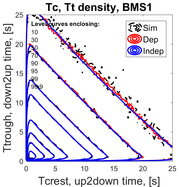
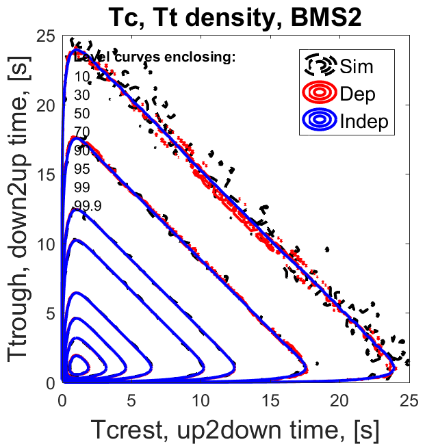
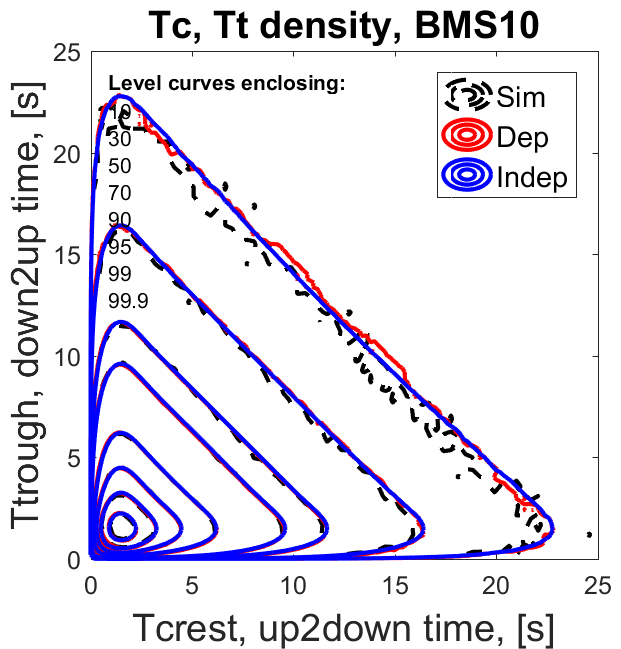
Figure 5: Joint pdf for crest-trough periods for Gaussian processes with with 1D, 2D, 10D diffusion type covariance BMSd.

4.2.2 Other spectra with near independent half periods

Figure 6 shows joint pdf for four different type spectra where successive intervals are near uncorrelated and almost pairwise independent, as measured by the Kullback-Leibler distance. There is clear visual agreement between the exact pdf (red) and the pdf with independent margins. The Gaussian spectrum WH0 and the approximating LH1 are centered at zero frequency and follow the IIA model almost perfectly. However, the white noise spectrum WN deviates considerable from how one normally envisages independent variables. The Butterworth spectrum BS approximates the WN spectrum and the pdf is near to independence. Note again that the marginal distributions are computed from the exact pdf by integration and not by the renewal argument as in the IIA approach.

4.2.3 Spectra with strongly dependent half periods

Figure LABEL:Fig:nonIIA shows examples with clear or even strong dependence. The spectrum LH7 is of the irregular type (21) with a small tendency of having three zeros close to each other, as shown by the red exact level curve near the origin. The three other spectra, the Jonswap, J and the shifted Gaussians, WH4, WH9, are regular with large regularity parameter $\alpha$, large correlation coefficients, and Kullback-Leibler difference larger than $0.1$. As is obvious from the figures the dependence can take many different shapes, which makes it difficult to catch it in a simple parametric form.

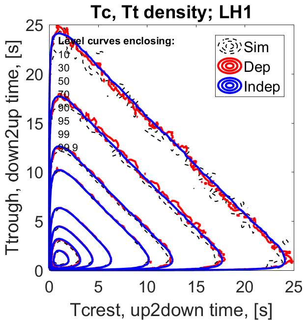
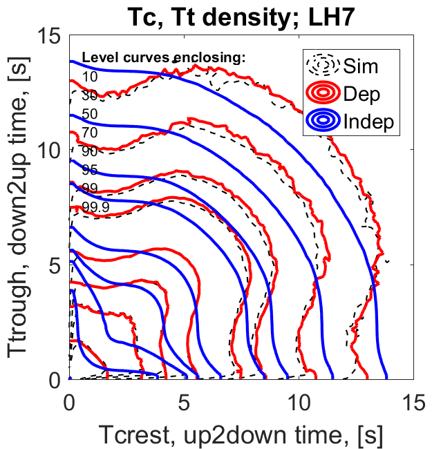
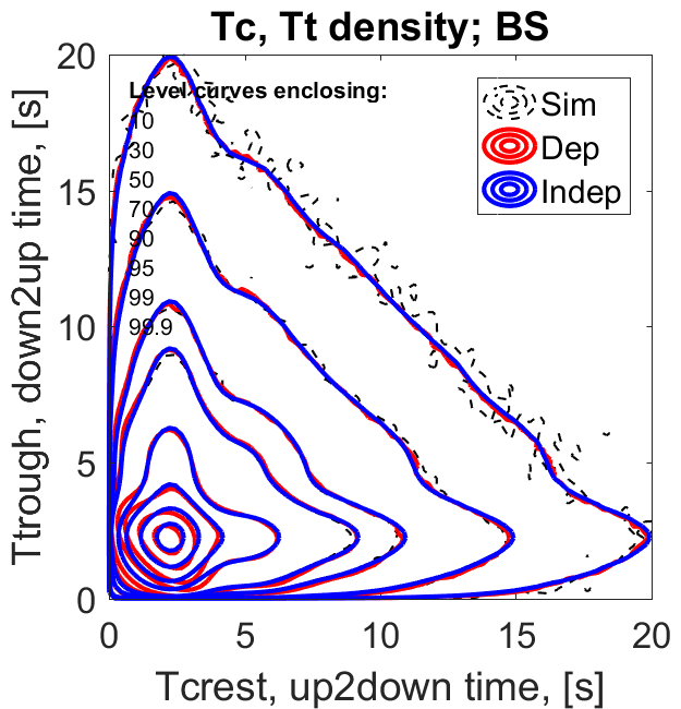
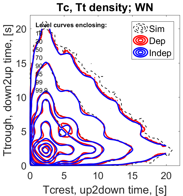
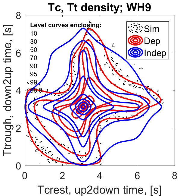
Figure 6: Joint pdf for spectra. The first two columns (left) almost independent half periods: LH1, WH0, BS, WN with correlation coefficient -0.02, -0.02, -0.02, -0.01 and Kullback-Leibler distance KL = 0.00, 0.00, 0.01, 0.04, respectively. The remaining two columns (right) spectra with clear dependence: : LH7, J, WH4, WH9 with correlation coefficient 0.13, 0.44, 0.30, 0.48 and Kullback-Leibler distance 0.05, 0.14, 0.11, 0.55, respectively. Level curves enclose 10, 30, …, 99.9 % of the distributions. Red solid curves: pdf computed by RIND; Blue solid curves: pdf under IIA assumption, with marginal pdf from RIND; Black dashed curves: simulated pdf from about 2.6 million pairs of crest-trough intervals.

4.3 Gaussian diffusion BMSd and the persistence exponent

The diffusion type covariance appears as a model for the diffusive time development of a Gaussian random field, initiated as white noise at time $t=0$. After a transformation to logarithmic time, $T=\log t$, the field is a stationary (homogeneous) Gaussian field with the $\operatorname{sech}^{d/2}(t/2)$ covariance function. Persistence for diffusion systems has been studied in physics since the early 1990s.

Majumdar et al., (1996) used the Independent Interval Assumption and (13) to find $\theta_{IIA}$ for different dimensions, and compared with simulations, while Wong et al., (2001) presented experimental evidence for $d=1$. Newman and Loinaz, (2001) designed an efficient simulation procedure to estimate the persistence probability for arbitrary dimension and suggest corresponding persistence exponents based on the simulations. Poplavskyi and Schehr, (2018) gives a definite answer for dimension $d=2$, namely $\theta(2)=3/16=0.1875$, a value that agrees with the Newman and Loinaz, (2001) simulation. At present, no exact values are known for other dimensions.

We can now compare these results with values computed by means of the RIND, which integrates the multidimensional normal density to give the tail probability $Q_{T}$ (9) for arbitrary interval length; Remark 1.

Our first concern is the shape of the distribution. In Section 4.2.1 we argued that the independence of successive intervals appears to be approximately satisfied for the diffusion spectra, Figure 5. The marginal distributions are rather close to exponential, even if not exactly so. What effect the deviation has on the persistence approximation $\theta_{IIA}$ from (13) is unclear. However, as shown in Appendix A.5.1, Table 4, and with agreement with earlier results in the literature, the resulting approximation of the persistency exponent is in the vicinity of 0.1863 which underestimated the true value 0.1875. Furthermore, the structure of the theoretical limiting behaviour (11) makes it difficult to estimate any persistence exponent by simulation or numerical computation.

Table 3: Numerically calculated persistence exponents $\theta(d)$ for diffusion. ^∗For the values in parenthesis, see text.

d NL RIND d NL RIND 1 0.1205 0.1206 (0.1203)^∗ 10 0.4587 0.4589 2 0.1875 0.1874 (0.1875)^∗ 20 0.6556 0.6561 3 0.2382 0.2382 30 0.8053 0.8063 4 0.2806 0.2805 40 0.9232 0.9327 5 0.3173 0.3171 50 1.0415 1.0439

The persistence estimates in (Newman and Loinaz,, 2001, Tab. 1) come from a large and well controlled simulation experiment of over $10^{8}$ realizations of first crossing events. We have designed the following numeric procedure to estimate the persistence exponent.

1. Fix a maximum $T_{m}$ and a grid $t_{k}=k\Delta$, $t_{m}\Delta=T_{m}$; this resembles the logarithmic grid in the Newman and Loinaz, (2001) simulations. $T_{m}$ should be chosen so large that any numeric or stochastic uncertainty in the tail is revealed.

2. Compute, with RIND, $Q_{T}$ for $T=t_{k},k=1,\ldots,m$; Newman and Loinaz, (2001) estimate $Q_{T}$ by simulation.

3. Make repeated independent runs to compute $Q_{T}$ and take the average $\overline{Q}_{T}$; RIND uses Monte Carlo integration for extreme cases, and averaging will reduce the stochastic uncertainty.

4. Make a regression of $-\log(2*\overline{Q}_{T})$ against $T$; this can be done globally, over the entire interval $[0,T_{m}]$ or locally to allow for slow asymptotics in (11). The persistence index is then estimated as the slope of the fit. We used quadratic polynomial fit to identify any typical trend in the exponential $e^{(\theta+A(T))T}$.

We used this scheme to estimate the persistence index for the 10 selected dimensions in (Newman and Loinaz,, 2001). We set $\Delta=0.05$ and $T_{m}=15$ for $d\geq 4$, which corresponds to the time span used in that paper and $\Delta=0.1$ and $T_{m}=30,30,20$ for $d=1,2,3$. We computed $\overline{Q}_{T}$ as the average of 400 independent runs of RIND with the SOBNIED method and highest precision. The quadratic fit indicated that the local slope increased slowly with $T$. Table 3 shows the local $\theta_{T}$ in the middle of the interval, $T=T_{m}/2$.

For dimensions $d=1,2$ we give two values in parenthesis to take account of the asymptotic character of the persistence exponent. To accomplish this, we increased $T_{m}$ to $40,35$, respectively and estimated the local rate of decay for large $T$. For $d=1$, the value $\theta=0.1206$ is the best estimates over the interval $(0,30)$, while the value $0.1203$ is the stable value for large $T$. The NL-value $0.1205$ is probably too high, based on a too short time span. The RIND-value $0.1203$ agrees with the value computed by IIA. For $d=2$ the stable value is $0.1875$, equal to the theoretical value $3/16$, Poplavskyi and Schehr, (2018).

       

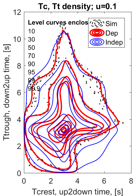
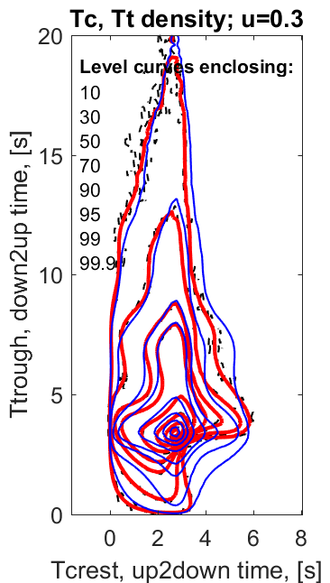
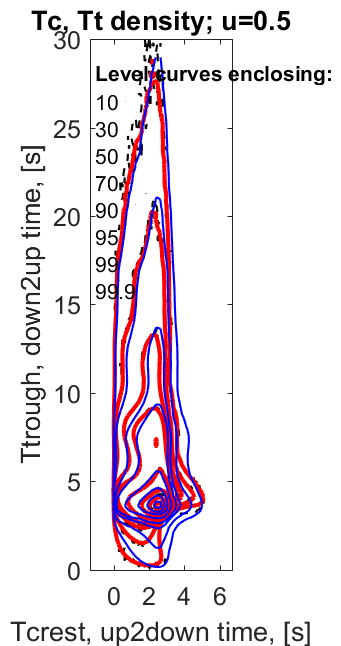
Figure 7: Joint pdf of interval above and below levels $u=0.1,0.3,0.5$ for shifted Gaussian spectrum WH6.

4.4 Crossings of non-zero levels

The RIND function is not limited to joint crest-trough period distribution but can be used for crossings of any level. We illustrate this on the Shifted Gaussian spectrum model WH6 for levels $u=0.1,0.3,0.5$. Figure 7 shows the dependence, and also the good agreement between the RIND results and simulated pdf:s, based on more than 2.2 million pairs of excursions.

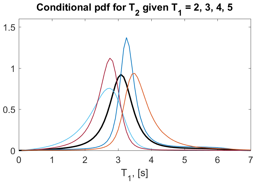
Figure 8: Crossing and conditional crossing densities for WH6. Black curve: marginal pdf for zero crossing interval; colour curves: conditional pdf for next interval given the first one, $T_{2}\mid T_{1}=2,3,4,5$.

4.5 The Markov approximation

The Markov approximation for zero crossing intervals dates back to McFadden, (1958) and Rainal, (1962, 1963), who also tested the model by means of the sequence of correlations. Having the exact joint distribution of successive zero crossing intervals a natural next step is to test the Markov chain dependence of the full sequence of crossing intervals. If $f_{T_{1},T_{2}}(t_{1},t_{2})$ is the joint density of two successive crossing intervals, one can construct a Markov transition kernel as $k(t_{2}\mid t_{1})=f_{T_{1},T_{2}}(t_{1},t_{2})/f_{T_{1}}(t_{1})$. Since the numerical algorithm gives the joint density in discretized form it is natural to construct a discrete Markov chain with discrete states $x_{1},x_{2},\ldots,x_{n}$ and transition matrix

$$\text{\sf P}(T_{2}=x_{k}\mid T_{1}=x_{j}) =\frac{f_{T_{1},T_{2}}(x_{j},x_{k})}{\sum_{k}f_{T_{1},T_{2}}(x_{j},x_{k})}.$$ (23)

Figure 8 illustrates he conditional pdf:s for the shifted Gaussian spectrum WH6 with clearly correlated crossing intervals, $\text{\sf Corr}(T_{1},T_{2})=0.40$. The figure shows the marginal pdf for a single zero crossing interval and four conditional pdf:s for a second interval given the length of the first. It is now possible to construct a Markov process with the transition matrix (23) and use it as an approximation for the distribution of the whole crossing sequence. A natural, exact, and rather strong test of the model can be based on the trivariate distribution of three consecutive intervals. The exact tri-variate density $f_{T_{1},T_{2},T_{3}}(t_{1},t_{2},t_{3})$ can be computed by RIND with the same degree of complexity as the bivariate density.

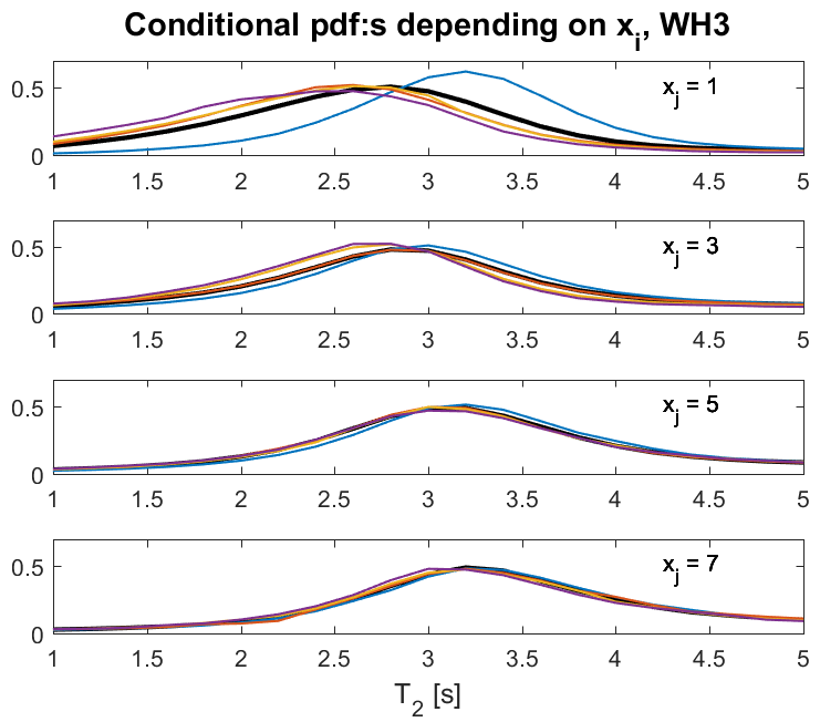
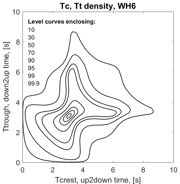
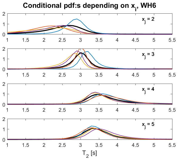
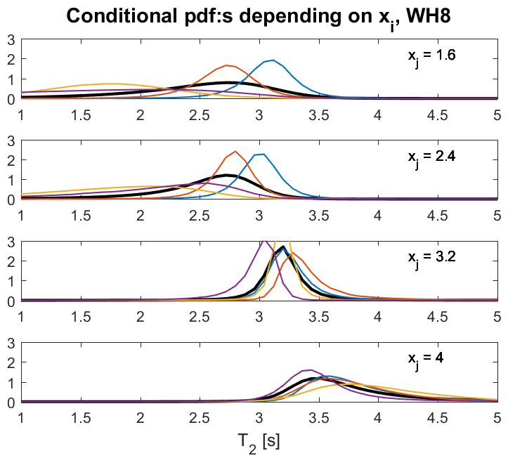
Figure 9: Markov tests. The top row for WH3, the middle for WH6 and the bottom for WH8. The left plot shows the 2D density of successive half periods. The right plot shows conditional densities for $T_{2}$, conditioned on the value of $T_{1}=x_{j}$ as black thick lines in each subplot. The coloured curves show the effect of also conditioning on the preceding $T_{0}$ taking any of the $x$ values.

If the crossing sequence is a Markov chain, then the conditional pdf of an interval $T_{2}$, given the length of the previous interval $T_{1}$, should be equal to its conditional pdf, given the lengths of the two previous ones $(T_{0},T_{1})$, i.e., for all $x_{i},x_{j},x_{k}$, the following equality should hold,

$$\text{\sf P}(T_{2}=x_{k}\mid T_{0}=x_{i},T_{1}=x_{j}) =\frac{f_{T_{0},T_{1},T_{2}}(x_{i},x_{j},x_{k})}{\sum_{i}f_{T_{0},T_{1},T_{2}}(x_{j},x_{k},x_{n})}=\text{\sf P}(T_{2}=x_{k}\mid T_{1}=x_{j}).$$ (24)

We illustrate the technique on the WH3, WH6, WH8 processes, as examples of processes with “almost independent”, “moderately dependent”, and “strongly dependent” successive intervals.

We use the RIND applications cov2ttpdf and cov2tttpdf to compute the 2D and 3D densities in (23) and (24) and then compute and plot the left hand sides conditional densities for selected values of $x_{j}$ and, for each $x_{j}$, for different $x_{i}$. Figure 9 shows the results.

The left plot in each figure shows the 2D density of successive half periods. The right plot shows conditional densities for $T_{2}$, conditioned on the value of $T_{1}=x_{j}$ as black thick lines in each subplot. The coloured curves show the effect of also conditioning on the preceding $T_{0}$ taking any of the $x$ values. For example, the blue curve is the conditional pdf, given $T_{0}=T_{1}=x_{1}$, etc.

From the figures, we can conclude that for WH3 the black curves are different, proving the dependence between intervals. However, the coloured curves in each subplot do not deviate much from the respective black curve, except for the shortest interval, which indicates that the Markov chain approximation can be used. For WH6 the deviation from a Markov model is stronger, and for WH8 the Markov model fails altogether.

5 Conclusions

Advances in statistical computing during recent decades has made it possible to compute probabilities and expectations in very high-dimensional nearly singular normal distributions. We have illustrated how the Matlab implementation RIND of these methods can be used to solve intricate level crossing problems in Gaussian processes.

We have shown how RIND is used to compute the bivariate distribution of the distance between three successive level crossings by a general stationary Gaussian process, based only on its covariance function. We have identified processes where successive intervals are almost independent, including diffusion related processes in different dimensions, where the “Independent Interval Approximation” (IIA) is expected to provide accurate results due to small correlation between subsequent crossing intervals. However even in this favorable situation, the IIA in 2D clearly underestimates ($\approx 0.1863$) the actual value of the persistency exponent (=0.1875), which is defined as the exponential rate with which the tail of the interval length distribution falls off. An additional problem with the IIA, when it utilizes the covariance matching, is that it does not yield a valid probability distribution. We conclude that the IIA has to be used with caution even in the cases when the independence is nearly valid.

On the other hand, we show that our algorithm works remarkably well both for obtaining the actual distribution of the crossing intervals but also in approximating the tail of the length distribution. We demonstrated it not only for the nearly independent interval cases, as we have also identified processes with strong dependence and very complex structure, including standard ocean wave models, shifted Gaussian spectra, and simple rational spectra. For these processes using the IIA is even more questionable, however the distributions computationally retrieved through RIND are matching very well the computationally intensive simulations from the process. We have also indicated how the method can be extended to deal with higher order dependence and Markov dependence.

The precision of the algorithm has been illustrated on the distribution of very long crossing intervals. For diffusion in 2D the RIND algorithm gives the correct theoretical value, and for other dimensions the results agrees with other large Monte Carlo studies.

Appendix A Appendix

A.1 Generalized Rice’s formula

The results in (1) and (16) given in Sections 2.1.1 and 3.1 can be shown using a generalized Rice’s formula presented in full generality in (Azaïs and Wschebor,, 2009, Thm. 6.4).

Theorem 1 (Weighted Rice Formula).

Let $Z:U\rightarrow R^{d}$ be a random field, $U$ an open subset of $R^{d}$, and $u\in R^{d}$ a fixed point. Assume that:

• $Z$ is Gaussian;

• almost surely the function $t\rightarrow Z(t)$ is of class $C^{2}$;

• for each $t\in U$, the distributtion of $Z(t)$ is non-degenerated, i.e. has a non-singular covariance matrix;

Then for $N_{\Lambda}(u)$, the number of $t$ in a compact $\Lambda\subset U$ such that $Z(t)=u$,

$$\text{\sf E}[N_{\Lambda}(u)]=\int_{\Lambda}\int|\det\dot{z}|f_{\dot{Z}(t),Z(t)}(\dot{z},u)\,\mathrm{d}\dot{z}\,\mathrm{d}t.$$ (25)

In addition, assume that for each $t\in U$ one has another field, $Y^{t}:W\rightarrow R^{n}$, defined on some topological space $W$, and verifying the following conditions:

• $Y^{t}(w)$ is a measurable function of $(\omega,t,w)$ and almost surely, $(\omega,t,w)\rightarrow Y^{t}(w)$ is continuous;

• for each $t\in U$ the random process $(t,w)\rightarrow(Z(t),Y^{t}(w))$ defined on $U\times W$ is Gaussian.

Then, if $g:U\times C(W,R^{n})\rightarrow R$ is a bounded and continuous function, when $C(W,R^{n})$ has the topology of uniform convergence on compact sets, then for each compact subset $\Lambda$ of U one has

$$\text{\sf E}\Bigg{[}\sum_{t\in\Lambda,Z(t)=u}g(t,Y^{t})\Bigg{]}=\int_{\Lambda}\text{\sf E}[|\det\dot{Z}(t)|g(t,Y^{t}))|Z(t)=u]f_{Z(t)}(u)\,\mathrm{d}t.$$ (26)

In the theorem, $Y^{t}(w)$ is an $n$-dimensional mark attached to time point $t$. When using the theorem on different crossing problems, we will refer to $n$ as the dimension of the problem.

There are more general versions of Rice’s formula, see Zähle, (1984) and Podgórski et al., (2000) shown under minimal assumptions on a random field. However the price is that they are valid for almost all levels $u$. Consequently the result shown in this appendix are also (in practice) applicable for any smooth, symmetrical, time reversible process, not necessarily Gaussian. We now demonstrate relations (1a), (1c), and (16) in this paper.

Let $X(t)$ be a standardized Gaussian process satisfying the assumptions of the generalized Rice’s theorem. We shall use the theorem to find the distributions of the variables $A,B$, and the ergodic distribution of $T$, the distance between consecutive zeros, and the formula for the joint probability density of two consecutive intervals between zeros, $T_{1},T_{2}$. Here we let $u=0$, however similar formulas can be shown to hold for any $u$.

Furthermore, previously used notation will be used, viz. $X_{s,t,u}=(X(s),X(t),X(u))$, $\dot{X}_{s,t,u}=(\dot{X}(s),\dot{X}(t),\dot{X}(u))$, $\dot{X}_{s,t,u}^{+-+}=\dot{X}(s)^{+}\dot{X}(t)^{-}\dot{X}(u)^{+}$, and $X_{s,t}=(u,v)$ means $X(s)=u,X(t)=v$. Moreover, $a\leq X_{s,t}\leq b$ means that for each $u\in(s,t):a\leq X(u)\leq b$, while $\{a\leq X_{s,t}\leq b\}$ also stands for the indicator function of this set, i.e. the function equal to one whenever the condition between the brackets is satisfied and to zero otherwise.

A.2 Probability density function of time to first crossing and stationary distribution of time between two zeros

A.2.1 Pdf of time $A$ to first zero crossing

Consider a zero mean stationary smooth Gaussian process $X(t)$ and take $u=0$. Let $Z(t)=X(t)$ and $Y^{t}(w)=X(w)$ so the dimension is $n=1$. (Note that $X$ has a.s. no local extremes with height equal zero.) Define $g$ as the indicator function equal to one if the process has a constant sign in the interval $(0,t)$, $g(t,Y^{t})=\{X_{0,t}>0\}+\{X_{0,t}<0\}$.

For $\Lambda=[0,a]$ the generalized Rice’s formula writes

$$\text{\sf E}\Bigg{[}\sum_{t\in\Lambda,Z(t)=u}g(t,Y^{t})\Bigg{]} =\int_{0}^{a}\text{\sf E}[|\dot{X}(t)|(\{X_{0,t}>0\}+\{X_{0,t}<0\})\mid X(t)=0]\,f_{X(t)}(0)\,\mathrm{d}t$$

$$=2\int_{0}^{a}\text{\sf E}[|\dot{X}(t)|\{X_{0,t}>0\}\mid X(t)=0]\,f_{X(t)}(0)\,\mathrm{d}t,$$

since $X$ is symmetrical around $0$. Now the weighted sum $\text{\sf E}\big{[}\sum_{t\in\Lambda,Z(t)=0}g(t,Y^{t})\big{]}$ is equal to the probability that $A\in\Lambda$, and hence the probability density of $A$ (and $B$) is given by

$$f_{A}(a) =2\text{\sf E}[\dot{X}(a)^{-}\{X_{0,a}>0\}\mid X(a)=0]\,f_{X(a)}(0)$$ (27)

$$=2\text{\sf E}[\dot{X}(0)^{-}\{X_{-a,0}>0\}\mid X(0)=0]\,f_{X(0)}(0)$$

$$=2\text{\sf E}[\dot{X}(0)^{+}\{X_{0,a}>0\}\mid X(0)=0]\,f_{X(0)}(0),$$ (28)

by time reversibility of $X$.

Observe that the function $g(t,Y^{t})$ is an indicator function and hence not continuous. Hence one needs to show that (26) is valid also for such a function $g$. This is done by employing the theorem for a sequence of continuous functions $g_{\epsilon}$, which converges to $g$ in such a way that a dominated or monotone convergence theorem can be applied. For example see the proof of Theorem 7.1 in Åberg et al., (2008). A similar approach can be used here to prove the presented results.

A.2.2 Cdf of inter-crossing distance $T$; proof of (1c)

We turn now to the ergodic (stationary) distribution of $T$, the distance between zeros of $X(t)$. Following Lindgren and Rychlik, (1991) we have that the tail probability is equal to

$$\text{\sf P}^{st}(T>t_{0})=\frac{\text{\sf E}[\mbox{number of $T^{+}_{i}\in[0,1]$ such that $T^{+}_{i+1}-T^{+}_{i}>t_{0}$}]}{\text{\sf E}[\mbox{number of $T_{i}^{+}\in[0,1]$}]}.$$

Now for fixed $t_{0}>0$, let $g(t,Y^{t})=\{X_{t,t+t_{0}}>0\}+\{X_{t,t+t_{0}}<0\}$

$$\text{\sf E}\Bigg{[}\sum_{t\in[0,1]Z(t)=u}g(t,Y^{t})\Bigg{]} =\int_{0}^{1}\text{\sf E}[|\dot{X}(t)|\{X_{t,t+t_{0}}>0\}+\{X_{t,t+t_{0}}<0\}\mid X(t)=0]\,f_{X(t)}(0)\,\mathrm{d}t$$

$$=2\text{\sf E}[\dot{X}(0)^{+}\{X_{0,t_{0}}>0\}\mid X(0)=0]\,f_{X(0)}(0),$$

by stationarity of $X$. Consequently by (28) the ergodic (stationary) distribution of $T$ satisfies the following relation

$$\text{\sf P}^{st}(T>t_{0})=\nu^{-1}\text{\sf E}[\dot{X}(0)^{+}\{X_{0,t_{0}}>0\}\mid X(0)=0]\,f_{X(0)}(0)=\mu f_{A}(t_{0}),$$ (29)

where $2\nu=1/\mu$ is the intensity of zeros. Hence the relation (1c) is shown.

The code for evaluation of the distribution of $T$ based on the above result and examples of evaluation for the diffusion in 2D is presented in the computational section of this Appendix, see Section A.6

A.3 Joint pdf of $A,B$ and pdf of $T$; proof of (1a)

In this problem $n=2$, $Z({\bf t})=Z(s,t)=(X(s),X(t))$, $s<0<t$. Further $\Lambda=[-b,0]\times[0,a]$ and $g({\bf t},Y^{\bf t})=\{X_{s,t}>0\}+\{X_{s,t}<0\}$. Then by Rice’s formula

$$\text{\sf E}\Bigg{[}\sum_{{\bf t}\in\Lambda,Z({\bf t})={\bf 0}}g({\bf t},Y^{{\bf t}})\Bigg{]}=\int_{-b}^{0}\int_{0}^{a}\text{\sf E}[|\det\dot{Z}({\bf t})|g({\bf t},Y^{{\bf t}}\mid X_{s,t}={\bf 0}]\,f_{X_{s,t}}({\bf 0})\,\mathrm{d}t\,\mathrm{d}s$$

$$\hskip 28.45274pt=2\int_{-b}^{0}\int_{0}^{a}\text{\sf E}[\dot{X}(s)^{+}\dot{X}(t)^{-}\{X_{s,t}>0\}\mid X_{s,t}={\bf 0]}\,f_{X_{s,t}}({\bf 0})\,\mathrm{d}t\,\mathrm{d}s.$$

Obviously the weighted sum $\text{\sf E}\big{[}\sum_{{\bf t}\in\Lambda,Z({\bf t})=0}g({\bf t},Y^{{\bf t}})\big{]}$ is equal to $\text{\sf P}(B\leq b,A\leq a)$. Hence the joint probability density of $B,A$ is given by

$$f_{B,A}(b,a) =2\text{\sf E}[\dot{X}(-b)^{+}\dot{X}(a)^{-}\{X_{-b,a}>0\}\mid X_{-b,a}={\bf 0}]\,f_{X_{-b,a}}({\bf 0})$$

$$=2\,\text{\sf E}[\dot{X}(0)^{+}\dot{X}(a+b)^{-}\{X_{0,a+b}>0\}\mid X_{0,a+b}={\bf 0}]\,f_{X_{0,a+b}}({\bf 0}),$$ (30)

$0<a,b$, by stationarity of $X$.

Next we give the pdf of the distribution in (29). Again $n=2$, but with $Z({\bf t})=Z(t,s)=(X(t),X(t+s))$, $\Lambda=[0,1]\times[0,t_{0}]$ and $g(t,Y^{\bf t})=\{X_{t,t+s}>0\}+\{X_{t,t+s}<0\}$. Obviously $\det\dot{Z}({\bf t})=\dot{X}(t)\dot{X}(t+s)$ and by Rice’s formula

$$E\Bigg{[}\sum_{{\bf t}\in\Lambda,Z({\bf t})={\bf 0}}g({\bf t},Y^{{\bf t}})\Bigg{]}=\int_{0}^{1}\int_{0}^{t_{0}}\text{\sf E}[|\det\dot{Z}({\bf t})|g({\bf t},Y^{{\bf t}})\mid X_{t,t+s}={\bf 0}]\,f_{X_{t,t+s}}({\bf 0})\,\mathrm{d}t\,\mathrm{d}s$$

$$\hskip 28.45274pt=2\int_{0}^{t_{0}}\text{\sf E}[\dot{X}(0)^{+}\dot{X}(s)^{-}\{X_{0,s}>0\}\mid X_{0,s}={\bf 0}]\,f_{X_{0,s}}({\bf 0})\,\mathrm{d}s,$$

by stationarity. Consequently the pdf of $T$ is given by

$$f_{T}(t)=\nu^{-1}\text{\sf E}[\dot{X}(0)^{+}\dot{X}(t)^{-}\{X_{0,t}>0\}\mid X_{0,t}={\bf 0}]\,f_{{X_{0},t}}({\bf 0}).$$ (31)

A comparison with (30) gives

$$f_{B,A}(b,a)=\mu^{-1}\,f_{T}(a+b),\quad 0<a,b,$$

and (1a) is proved, since $2\nu=1/\mu$. Note that in both the presented examples the probability density function of $Z(t,s)$ is not bounded for all $(s,t)\in\Lambda$. This is only a technical problem which is solved by replacing the interval $[0,t_{0}]$ in the definitions of $\Lambda$ by $[\varepsilon,t_{0}]$, $\varepsilon>0$ and then letting $\varepsilon$ tend to zero.

A.4 Stationary joint probability density function of $(T_{1},T_{2})$

Now $n=3$ and ${\bf t}=(r,t,s)$, $Z({\bf t})=(X(t+r),X(t),X(t+s))$. Furthermore we let $Y^{\bf t}(\tau)=X(\tau)$ and $\Lambda=[t_{1},0]\times[0,1]\times[0,t_{2}]$ and for $r<0<s$

$$g({\bf t},Y^{\bf t})=\{X_{t+r,t}<0\}\{X_{t,t+s}>0\}+\{X_{t+r,t}>0\}\{X_{t,t+s}<0\}.$$

Since $\det\dot{Z}({\bf t})=\dot{X}(t+r)\dot{X}(t)\dot{X}(t+s)$ and by symmetry of $X$ around level zero, Rice’s formula gives

$$\text{\sf E}\Bigg{[} \sum_{{\bf t}\in\Lambda,Z({\bf t})=0}\,g({\bf t},Y^{{\bf t}})\Bigg{]}=\int_{t_{1}}^{0}\int_{0}^{1}\int_{0}^{t_{2}}\text{\sf E}[|\det\dot{Z}({\bf t})|g({\bf t},Y^{\bf t})\mid Z({\bf t})={\bf 0}]\,f_{Z({\bf t})}({\bf 0})\,\mathrm{d}r\,\mathrm{d}t\,\mathrm{d}s$$

$$=2\int_{t_{1}}^{0}\int_{0}^{t_{2}}\text{\sf E}[\dot{X}(r)^{-}\dot{X}(0)^{+}\dot{X}(s)^{-}\{X_{r,0}<0\}\{X_{0,s}>0\}\mid X_{r,0,s}={\bf 0}]\,f_{X_{r,0,s}}({\bf 0})\,\mathrm{d}r\,\mathrm{d}s,$$

by stationarity and hence the joint probability density function of $T_{1}<0<T_{2}$ is

$$f_{T_{1},T_{2}}(t_{1},t_{2})=\nu^{-1}\,\text{\sf E}[\dot{X}(t_{1})^{-}\dot{X}(0)^{+}\dot{X}(t_{2})^{-}\{X_{t_{1},0}<0\}\{X_{0,t_{2}}>0\}\mid X_{t_{1},0,t_{2}}=({\bf 0})]\,f_{X_{t_{1},0,t_{2}}}({\bf 0}),$$

in agreement with (16).

A.5 The validity of the IIA

In this appendix we consider the inverse problem, that constitutes a basis for the IIA approach. Namely, for a given covariance function $R$, normalized so that $R(0)=1$, we ask whether the function $\Psi$ defined through

$$\Psi(s)=\frac{2-s\mu(1-s\mathcal{L}R(s))}{2+s\mu(1-s\mathcal{L}R(s))}=\frac{2}{1+\frac{\mu}{2}(s-s^{2}\mathcal{L}R(s))}-1,$$ (32)

for a certain $\mu>0$ corresponds to the Laplace transform of a probability distribution function of a non-negative random variable.

We recall that by Bernstein’s theorem the function $\Psi$ is a Laplace transform of a probability distribution on the positive half-line if and only if $\Psi(0)=1$, it has all derivatives on $(0,\infty)$ and

$$(-1)^{n}\Psi^{(n)}(s)\geq 0,~{}~{}s>0.$$

It is not difficult to verify that the function given in (32) takes value one at $s=0$ and it satisfies the above for $n=0$. However, as we will see next, covariances $R$ that lead to a valid probability distributions are restricted only to ones that have a singular component in their spectral measure, the requirement that is rarely satisfied for covariances of interest. In particular for Gaussian processes considered in this work, $\Psi$ is not the Laplace transform of a probability distribution. We first formulate this result and then provide the argument through some auxiliary facts of a more general nature.

Proposition 1.

Let $X$ be a Gaussian process with the (symmetric) spectrum $S$, i.e. its covariance is given by

$$r(t)=\int_{-\infty}^{\infty}e^{i\omega t}S(\omega)\,\mathrm{d}\omega.$$

Then for the covariance $R=R_{0}^{c}$ of the clipped process $D_{c}(t)=\operatorname{sgn}(X(t))$ that has the form

$$R(t)=\frac{2}{\pi}\arcsin(r(t)/r(0)),$$

the function $\Psi$ given through (32) does not represent a valid probability distribution for any choice of $\mu>0$.

Remark 2.

We note that most of physically interpretable processes are given by a symmetric spectrum, including these in Table 1. In particular, the diffusion process in dimension two has the explicit spectrum $S(\omega)=\operatorname{sech}(\pi\omega)$.

The argument that shows the above conclusions is based on discussing when the Bernstein condition for $n=1$ can be satisfied by $\Psi$, i.e. for $s>0$ we investigate if

$$-\Psi^{\prime}(s) =\mu\frac{1-2s\mathcal{L}R(s)-s^{2}\mathcal{L}R^{\prime}(s)}{\left(1+\frac{\mu}{2}s^{2}(1/s-\mathcal{L}R(s))\right)^{2}}\geq 0.$$

By Bochner’s theorem any covariance $R$ can be written in terms of its spectral measure $S_{R}$ as

$$\int_{-\infty}^{\infty}e^{it\omega}\,\mathrm{d}S_{R}(\omega).$$

From this we have

$$\mathcal{L}R(s) =2\int_{0}^{\infty}\frac{s}{s^{2}+\omega^{2}}\,\mathrm{d}S_{R}(\omega),$$

$$\mathcal{L}R^{\prime}(s) =2\int_{0}^{\infty}\frac{\omega^{2}-s^{2}}{s^{2}+\omega^{2}}\,\mathrm{d}S_{R}(\omega),$$

and, by straightforward calculation, the necessary condition for a covariance $R(t)=\int_{-\infty}^{\infty}e^{i\omega t}\,\mathrm{d}S_{R}(\omega)$ to be obtained as a covariance of a switching process is

$$\mbox{}\int_{0}^{\infty}\frac{(\omega/s)^{4}}{\left(1+(\omega/s)^{2}\right)^{2}}\,\mathrm{d}S_{R}(\omega)\geq\int_{0}^{\infty}\frac{1+4(\omega/s)^{2}}{\left(1+(\omega/s)^{2}\right)^{2}}\,\mathrm{d}S_{R}(\omega),$$ (33)

an inequality that has to be satisfied for each $s>0$.

Let us consider now that $\mathrm{d}S_{R}(\omega)=S_{R}(\omega)\,\mathrm{d}\omega$. Since the normalized spectrum $S_{R}$ integrates to one (variance of the symmetric switching process is always one), there exists $K>0$ such that for all $s>K$ we have

$$\int_{0}^{s}S_{R}(\omega)\,\mathrm{d}\omega>4\int_{s}^{\infty}S_{R}(\omega)\,\mathrm{d}\omega.$$

Then for $s>K$ we have

$$\int_{0}^{\infty}\frac{u^{4}-1-4u^{2}}{(1+u^{2})^{2}}S_{R}(us)\,\mathrm{d}u =\int_{0}^{1}\frac{u^{4}-1-4u^{2}}{(1+u^{2})^{2}}S_{R}(us)\,\mathrm{d}u+\int_{1}^{\infty}\frac{u^{4}-1-4u^{2}}{(1+u^{2})^{2}}S_{R}(us)\,\mathrm{d}u$$

$$\leq-\int_{0}^{1}\frac{S_{R}(us)}{(1+u^{2})^{2}}\,\mathrm{d}u+\int_{1}^{\infty}S_{R}(us)\,\mathrm{d}u,$$

where the last integral appears because $(u^{4}-1-4u^{2})/(1+u^{2})^{2}<1$. Further,

$$\int_{0}^{\infty}\frac{u^{4}-1-4u^{2}}{(1+u^{2})^{2}}S_{R}(us)\,\mathrm{d}u \leq-\frac{1}{4}\int_{0}^{1}S_{R}(us)\,\mathrm{d}u+\int_{1}^{\infty}S_{R}(us)\,\mathrm{d}u$$

$$=\frac{1}{4s}\left(4\int_{s}^{\infty}S_{R}(\omega)\,\mathrm{d}\omega-\int_{0}^{s}S_{R}(\omega)\,\mathrm{d}\omega\right)<0.$$

This proves the following result.

Proposition 2.

If the covariance $R$ in (32) is given by a spectrum through

$$\int_{-\infty}^{\infty}e^{it\omega}S_{R}(\omega)\,\mathrm{d}\omega,$$

then the formula does not yield $\Psi$ corresponding to a probability distribution for any $\mu>0$.

To obtain Proposition 1 from the above arguments it is enough to show that the covariance given through

$$R(t)=\frac{2}{\pi}\arcsin(r(t)/r(0)),$$

has a continuous spectrum $S_{R}$ whenever $r$ has such. This follows from the series expansion

$$\operatorname{arcsin}z=z+\frac{1}{2}\frac{z^{3}}{3}+\frac{1\cdot 3}{2\cdot 4}\frac{z^{5}}{5}+\frac{1\cdot 3\cdot 5}{2\cdot 4\cdot 6}\frac{z^{7}}{7}+\cdots,$$

that implies that for the (normalized) spectrum $S_{r}$ of $r(t)/r(0)$ the spectrum of $R$ is given by

$$S_{R}=\frac{2}{\pi}\left(S_{r}+\frac{1}{2}\frac{S_{r}^{*3}}{3}+\frac{1\cdot 3}{2\cdot 4}\frac{S_{r}^{*5}}{5}+\frac{1\cdot 3\cdot 5}{2\cdot 4\cdot 6}\frac{S_{r}^{*^{7}}}{7}+\cdots\right).$$

A.5.1 Diffusion in dimension two

We illustrate the problem of recovering the crossing interval distribution by the IIA approach through the analysis of the diffusion in dimension two, with covariance as given in BMS2. This example can serve as the benchmark case since a lot of computation can be made more explicit and the actual value of persistency $\theta(2)=3/16=0.1875$ has been recently established in Poplavskyi and Schehr, (2018).

First, we report the following Laplace transform of the covariance obtained through a series expansion of $\displaystyle\arcsin x$,

$$\mathcal{L}\left(\frac{2}{\pi}\arcsin\left(\frac{2}{e^{t/2}+e^{-t/2}}\right)\right)(s)=\mbox{\large$\displaystyle\frac{2}{\pi}\sum_{l=0}^{\infty}$}~{}\frac{\displaystyle\sum_{k=0}^{l}\frac{1}{2^{k}(2k+1)}\binom{l+k}{k}\binom{s-1/2+k}{k}}{\displaystyle 2^{l}(l+1)\binom{s+1/2+l}{l+1}},$$

where

$$\binom{x}{y}=\frac{\Gamma(x+1)}{\Gamma(x-y+1)\Gamma(y+1)}.$$

We note the following structure:

$$\mathcal{L}\left(\frac{2}{\pi}\arcsin\left(\frac{2}{e^{t/2}+e^{-t/2}}\right)\right)(s)=\sum_{l=0}^{\infty}\frac{P_{l}(s)}{(s+1/2)\dots(s+1/2+l)},$$

where $P_{l}$ are polynomials in $s$ of the order $l$, given by

$$P_{l}(s)=\frac{l!}{\pi 2^{l-1}}\left(1+\sum_{k=1}^{l}\frac{\binom{l+k}{k}}{2^{k}(2k+1)k!}{(s+1/2)\dots(s+1/2+k-1)}\right).$$

Consequently, any partial sum that approximates the Laplace transform,

$$\mathcal{L}_{L}(s)=\sum_{l=0}^{L}\frac{P_{l}(s)}{(s+1/2)\dots(s+1/2+l)}=\frac{Q_{L}(s)}{(s+1/2)\dots(s+1/2+L)},$$

is also a rational function with the numerator being a polynomial in $s$ of order $L$, say $Q_{L}(s)$, while the denominator is a factorized polynomial of order $L+1$. This leads to the following approximate formula for the Laplace transform of the distribution of the crossing intervals,

$$\Psi_{L}(s) =\frac{4(s+1/2)\dots(s+1/2+L)}{(2+s\mu)(s+1/2)\dots(s+1/2+L)-\mu s^{2}Q_{L}(s)}-1.$$ (34)

We note that the first term is a ratio of two polynomials, with the numerator of order $L$ and denominator of order $L+1$. We immediately conclude that this cannot be a Laplace transform of a probability distribution since the function equal to minus one is the Laplace transform of a negative atomic measure with atom minus one at zero, while the ratio of the polynomials with the order of the numerator smaller than that of the denominator is incapable of canceling this negative atomic measure.

For the diffusion in D2, the recommended value of $\mu$ is $2\pi$ which is the average value of the zero crossing interval. We mark here that since the actual measure corresponding to $\Psi(s)$ is not probabilistic, this choice of $\mu$ is only partially justified.

Consider, for example, $L=0$. Direct computations leads to the following zero order approximation

$$\Psi_{0}(s) =\left(\frac{a}{s-s_{1}}+\frac{b}{s-s_{2}}\right)-1,$$

where

$$a \approx 0.2740,~{}~{}b\approx 1.4779$$

$$s_{1} \approx-0.2150,~{}~{}s_{2}\approx-2.0369$$

and the corresponding “distribution” that is obtained from the inverse Laplace transform has the absolute continuous part given by the density

$$f(t)=ae^{ts_{1}}+be^{ts_{2}}.$$

We point out that the inverse Laplace method does not produce a probabilistic measure due to the atom at zero although the total mass is still equal to one. The equivalent to the expectation is equal to $\mu=2\pi$ but it cannot be interpreted as the average value of the crossing interval. The “cdf” of this measure is presented in Figure 10. Finally, we note that the asymptotics is governed by the exponent $-s_{1}\approx 0.2150$, which could be viewed as a crude ($L=0$) approximation of the persistency exponent.

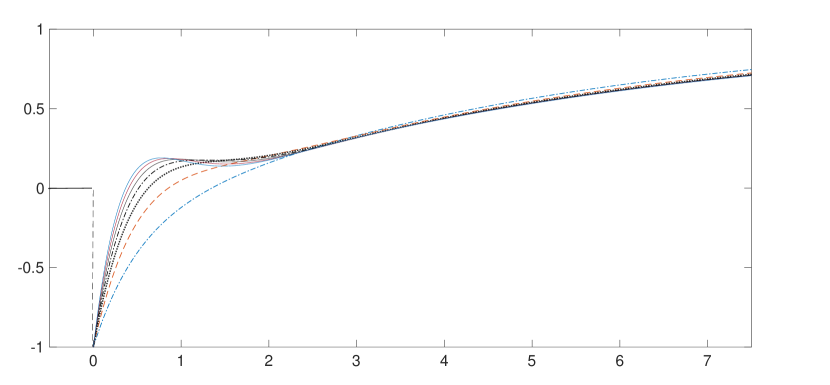
Figure 10: Several cumulative non-probabilistic distributions representing signed measures obtained through approximation (34) for $L=0,1,2,3,4,5,6$. The higher order approximations attempt to correct the high ‘bump’ near the origin.

Approximations for other values of $L$ can be done similarly. The obtained graphs of the quasi cumulative distribution functions are shown in Figure 10. It can be seen that there is a probabilistically uninterpretable negative jump at zero, which higher order approximations attempt to ‘correct’. This however leads to a probabilistically uninterpretable loss of the monotonicity on the continuous part for small values of the time crossings. However, as previously reported in the literature, the approach gives a reasonable estimate of the tail of the distribution as can be seen in the obtained persistency coefficients. In Table 4, we show the approximated values of the persistency coefficient. Recall that by a recent result in Poplavskyi and Schehr, (2018), the true persistency for the diffusion in two dimensions is $\alpha=3/16=0.1875$. We observe that this value very closely followed by even low order approximations and is actually attained by the approximation of order six. However, further approximations are producing smaller values eventually stabilizing at $\theta_{IIA}=0.1863$, which is consistent with the results reported in Bray et al., (2013) and Majumdar et al., (1996). Our conjecture is that this is the actual value of the persistency obtained by the IIA approach and thus it underestimates the actual value of the parameter.

Table 4: The approximated values of the persistency $\theta_{L}$ using the largest negative poles of $\Psi_{L}$ given in (34).

$L$	0	1	2	3	4	5	6	7
$\theta_{L}$	0.2150	0.1991	0.1930	0.1902	0.1887	0.1880	0.1875	0.1872
$L$	8	9	10	15	20	30	50	80
$\theta_{L}$	0.1870	0.1869	0.1868	0.1866	0.1865	0.1863	0.1863	0.1863

A.6 Examples of the code for some numerical results

In this section, for the reader and potential user convenience, we provide a complete code of some numerical evaluation presented in the paper using the WAFO-package.

The first code shows computation of the distribution of the time $T$ between subsequent crossings. In Figure 11, the resulting cdf in the normal and logarithmic scales is presented.

⬇

1% Script to compute the persistence, 1-cdf of intercrossing time

2dt=0.2; N=; t=0:dt:N*dt;

3Rt=sech(t/2);

4Rt1=tanh(t/2).*sech(t/2)/2;

5Rt2=(tanh(t(1)).*Rt1(1)+Rt(1).*(1-tanh(t(1)/2).^2)/2)/2;

6

7R=[toeplitz(Rt(1:end-1)); fliplr(Rt1(2:end))];

8R=[R [R(end,1:end) Rt2]’];

9R=[R;[fliplr(Rt(2:end))␣0]];

10R=[R␣[R(end,1:end)␣Rt(1)]’];

11

12%␣Set␣lower␣and␣upper␣bounds␣and␣compute␣P,␣prob␣to␣stay␣between␣bounds

13u=0;␣Blo=[u␣0];␣Bup=[inf␣inf];

14Pt=[];

15for␣i=1:N

16␣␣␣␣Nt=N-i+1;␣xc=u;␣indI=[0␣Nt␣Nt+1];␣mi␣=␣zeros(Nt+2,1);

17␣␣␣␣P=rind(R(i:end,i:end),mi,Blo,Bup,indI,xc,Nt);

18␣␣␣␣Pt=␣[Pt;␣[t(Nt+1)␣P]];

19end

20mu=sqrt(Rt2/Rt(1))/2/pi;

21Pt(:,2)=Pt(:,2)/mu;

22Pt=[Pt;[0␣1]];

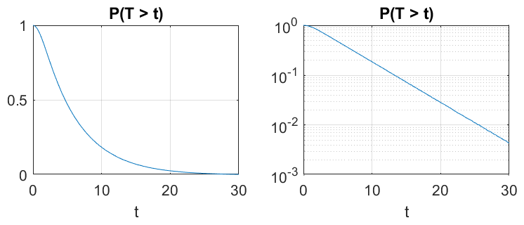
Figure 11: $P(T>t)$ for diffusion BMS2 computed by RIND, in the regular scale (Left) and in the logarithmic scale (Right).

In the next block of Matlab-code, some other computational results used across the paper are presented to illustrate relative simplicity of utilizing RIND. For description of the special command rindopset see the help text in WAFO.

⬇

1function [f,find] = cov2ttpdf_cov(cc,level,paramt,modify,varargin)

2%COV2TTPDF computes bivariate (Tc,Tt)

3%

4% CALL [f,find] = cov2ttpdf_cov(c,level,paramt,modify,options)

5%

6% f = 2D pdf structure for pair of crest/trough period

7% find = 2D pdf structure with assumed independent marginals

8%

9% c = symbolic covariance function

10% level = reference level, default = 0

11% paramt = [Tc Td Nc Nd] = [real real integer integer]

12% max crest/trough period and subdivision

13% with Nc/Nt = Tc/Td (if not, Tc,Td will be adjusted)

14% Default: Tc = Td = 10, Nc = Nd = 20 gives

15% pdf at x1,x2 = 0:0.5:10

16% modify = 1, modify irregular case (when L3 neq 0)

17% 0, do not modify (default)

18% options = options for RIND, set by rindoptset

19%

20% Use spec2ttsim to simulate half and full periods

21

22% History:

23% Updated 2018 and 2019 to allow irregular spectra

24% Revised by GL May 2017 - the input c (covariance function

25% or spectrum structure) is now normalized automatically to

26% m0 = m2 = 1

27% Made by Georg Lindgren, February 2017,

28% based on IR, PAB, KP and others spec2tpdf WAFO routine

29% Used on Matlab 2017b

30

31start = clock;

32narginchk(1,inf)

33

34defaultSpeed = 2;

35defaultMethod = 5;

36defaultoptions = rindoptset(’speed’,defaultSpeed,’method’,defaultMethod);

37if␣nargin<5

38␣␣␣␣␣␣␣␣opt␣=␣defaultoptions;

39else

40␣␣␣␣opt␣=␣rindoptset(defaultoptions,varargin{:});

41end

42

43if␣nargin␣<␣4␣||␣isempty(modify)

44␣␣␣␣modify␣=␣false;

45elseif␣modify␣==␣1

46␣␣␣␣modify␣=␣true;

47else

48␣␣␣␣modify␣=␣false;

49end

50if␣nargin<3␣||␣isempty(paramt)

51␣␣␣␣paramt␣=␣[10␣10␣20␣20];

52end

53if␣␣nargin␣<␣2␣||␣isempty(level)

54␣␣␣␣u␣=␣0;

55else

56␣␣␣␣u␣=␣level;

57end

58

59T1␣=␣paramt(1);␣%␣Aimed␣max␣crest␣interval

60T2␣=␣paramt(2);␣%␣Aimed␣max␣trough␣interval

61Nc␣=␣paramt(3);␣%␣Nc+1␣=␣length(x1)

62Nt␣=␣paramt(4);␣%␣Nt+1␣=␣length(x2)

63Ttot␣=␣T1+T2;

64Ntot␣=␣Nc+Nt;

65TimeStep␣=␣Ttot/Ntot;

66T1␣=␣Nc*TimeStep;␣%␣Final␣max␣crest␣interval

67T2␣=␣Nt*TimeStep;␣%␣Final␣max␣trough␣interval

68

69c␣=␣cc;

70covtxt␣=␣formula(c);

71

72%%%%%%%%%%%%%%%%%%%%%%%%%%%%%%%%%%%%%%%%%%%%%%%%%%%%%%

73%␣Create␣pdf-structure␣and␣prepare␣for␣information

74␣␣␣␣f␣=␣createpdf(2);

75␣␣␣␣f.labx{1}␣=␣’Tcrest,␣up2down␣time,␣[s]’;

76␣␣␣␣f.labx{2}␣=␣’Ttrough,␣down2up␣time,␣[s]’;

77␣␣␣␣f.title␣=␣’Tc,␣Tt␣density’;

78␣␣␣␣f.level␣=␣level;

79␣␣␣␣f.note␣=␣[’cov␣=␣’␣char(covtxt)];

80␣␣␣␣f.date␣=␣start;

81␣␣␣␣f.x{1}␣=␣linspace(0,T1,Nc+1);

82␣␣␣␣f.x{2}␣=␣linspace(0,T2,Nt+1);

83␣␣␣␣f.f␣=␣zeros(Nc+1,Nt+1);

84␣␣␣␣time␣=␣linspace(0,T1+T2,Nc+Nt+1);

85%␣End:␣Create␣pdf-structure

86

87%%%%%%%%%%%%%%%%%%%%%%%%%%%%%%%%%%%%%%%%%%%%%%%%%%%%%%

88%␣Compute␣R␣=␣covariance␣function␣and␣two␣derivatives

89%␣from␣symbolic␣covariance␣function␣and␣normalize␣to␣L0␣=␣L2␣=␣1

90%␣Note␣that␣irregular␣case␣is␣allowed

91␣␣␣␣syms␣t␣normedt

92␣␣␣␣L2_␣=␣diff(c,2);

93␣␣␣␣L2_␣=␣limit(L2_,0);

94␣␣␣␣korr␣=␣sqrt(-L2_);

95␣␣␣␣normedt␣=␣t/korr;

96␣␣␣␣c(t)␣=␣cc(normedt);

97

98␣␣␣␣ttp=time(time>0);

99␣␣␣␣dt␣=␣ttp(2)-ttp(1);

100␣␣␣␣t=sym(ttp);

101␣␣␣␣R.t=time;

102␣␣␣␣y=c(t);

103␣␣␣␣y0=limit(c,0);

104␣␣␣␣R.R=[double(y0)␣double(y)];

105␣␣␣␣L0=double(y0);

106

107␣␣␣␣dc=diff(c,1);

108␣␣␣␣y=dc(t);

109␣␣␣␣y0=limit(dc,0);

110␣␣␣␣R.Rt=[double(y0)␣double(y)];

111␣␣␣␣L1=double(y0);

112

113␣␣␣␣ddc=diff(c,2);

114␣␣␣␣y=ddc(t);

115␣␣␣␣y0=limit(ddc,0);

116␣␣␣␣R.Rtt=[double(y0)␣double(y)];

117␣␣␣␣L2␣=␣-double(y0);

118

119␣␣␣␣dddc=diff(c,3);

120␣␣␣␣syms␣t

121␣␣␣␣L3=double(limit(dddc,t,0,’right’));

122␣␣␣␣%Case␣is␣irregular␣if␣␣L3␣not␣equal␣0

123

124␣␣␣␣ddddc=diff(c,4);

125␣␣␣␣L4=double(limit(ddddc,t,0,’right’));

126%␣End:␣Covariances␣from␣symbolic␣covariance␣function

127

128%%%%%%%%%%%%%%%%%%%%%%%%%%%%%%%%%%%%%%%%%%%%%%%%%%%%%%%

129%␣Compute␣all␣covariance␣matrices␣for␣process␣and␣derivative

130␣␣␣␣R11␣=␣R.R(1:end);

131␣␣␣␣R11␣=␣toeplitz(R11);

132␣␣␣␣R22␣=␣-R.Rtt(1:end);

133␣␣␣␣R22␣=␣toeplitz(R22);

134␣␣␣␣R12␣=␣toeplitz(R.Rt(1:end));

135␣␣␣␣R12␣=␣diag(diag(R12))␣+␣triu(R12,1)␣-␣tril(R12,-1);

136␣␣␣␣R21␣=␣R12’;

137%␣End:␣Compute␣all␣covariance␣matrices

138

139%%%%%%%%%%%%%%%%%%%%%%%%%%%%%%%%%%%%%%%%%%%%%%%%%%%%%%%

140%␣Prepare␣for␣RIND

141␣␣␣␣Xc␣=␣zeros(3,1);

142␣␣␣␣Mine=100;␣ERR␣=␣zeros(Nc,Nt);␣TERR␣=␣zeros(Nc,Nt);

143␣␣␣␣tstart␣=␣tic;

144%␣End:␣Prepare␣for␣RIND

145

146%%%%%%%%%%%%%%%%%%%%%%%%%%%%%%%%%%%%%%%%%%%%%%%%%%%%%%%

147%␣Run␣RIND␣for␣all␣point␣in␣2D␣grid

148for␣j=1:Nc

149␣␣␣␣waitbar(j/Nc)

150␣␣␣␣for␣k␣=␣1:Nt

151␣␣␣␣%␣Select␣sub-covariance␣matrices␣from␣RRR

152␣␣␣␣Btt␣=␣[R11(j+1:Nc,j+1:Nc)␣␣␣␣␣␣␣␣␣-R11(j+1:Nc,Nc+2:Nc+Nt+1-k);

153␣␣␣␣␣␣␣␣␣␣-R11(Nc+2:Nc+Nt+1-k,j+1:Nc)␣␣R11(Nc+2:Nc+Nt+1-k,Nc+2:Nc+Nt+1-k)];

154

155␣␣␣␣Btd␣=␣[R12(j+1:Nc,j)␣-R12(j+1:Nc,Nc+1)␣R12(j+1:Nc,Nc+Nt+2-k)␣;

156␣␣␣␣␣␣␣␣␣␣-R12(Nc+2:Nc+Nt+1-k,j)␣␣R12(Nc+2:Nc+Nt+1-k,Nc+1)␣…

157␣␣␣␣␣␣␣␣␣␣␣␣␣␣␣␣␣-R12(Nc+2:Nc+Nt+1-k,Nc+Nt+2-k)];

158

159␣␣␣␣Btc␣=␣[R11(j+1:Nc,j)␣␣R11(j+1:Nc,Nc+1)␣␣R11(j+1:Nc,Nc+Nt+2-k);

160␣␣␣␣␣␣␣␣␣␣-R11(Nc+2:Nc+Nt+1-k,j)␣-R11(Nc+2:Nc+Nt+1-k,Nc+1)␣…

161␣␣␣␣␣␣␣␣␣␣␣␣␣␣␣␣␣␣-R11(Nc+2:Nc+Nt+1-k,Nc+Nt+2-k)];

162

163␣␣␣␣Bdd␣=␣[R22(j,j)␣␣␣␣␣␣␣␣␣-R22(j,Nc+1)␣␣␣␣␣␣␣␣␣␣R22(j,Nc+Nt+2-k);

164␣␣␣␣␣␣␣␣␣␣-R22(Nc+1,j)␣␣␣␣␣␣␣R22(Nc+1,Nc+1)␣␣␣␣␣␣-R22(Nc+1,Nc+Nt+2-k);

165␣␣␣␣␣␣␣␣␣␣R22(Nc+Nt+2-k,j)␣-R22(Nc+Nt+2-k,Nc+1)␣␣R22(Nc+Nt+2-k,Nc+Nt+2-k)];

166

167␣␣␣␣Bdc␣=␣[R21(j,j)␣␣␣␣␣␣␣␣␣R21(j,Nc+1)␣␣␣␣␣␣␣␣␣R21(j,Nc+Nt+2-k);

168␣␣␣␣␣␣␣␣␣␣-R21(Nc+1,j)␣␣␣␣␣-R21(Nc+1,Nc+1)␣␣␣␣␣-R21(Nc+1,Nc+Nt+2-k);

169␣␣␣␣␣␣␣␣␣␣␣R21(Nc+Nt+2-k,j)␣R21(Nc+Nt+2-k,Nc+1)␣R21(Nc+Nt+2-k,Nc+Nt+2-k)];

170

171␣␣␣␣Bcc␣=␣[R11(j,j)␣␣␣␣␣␣␣␣␣␣R11(j,Nc+1)␣␣␣␣␣␣␣␣␣R11(j,Nc+Nt+2-k);

172␣␣␣␣␣␣␣␣␣␣␣R11(Nc+1,j)␣␣␣␣␣␣␣R11(Nc+1,Nc+1)␣␣␣␣␣␣R11(Nc+1,Nc+Nt+2-k);

173␣␣␣␣␣␣␣␣␣␣␣R11(Nc+Nt+2-k,j)␣␣R11(Nc+Nt+2-k,Nc+1)␣R11(Nc+Nt+2-k,Nc+Nt+2-k)];

174

175␣␣␣␣␣␣␣␣BBB␣=␣[Btt␣␣Btd␣␣Btc;

176␣␣␣␣␣␣␣␣␣␣␣␣␣␣␣Btd’␣Bdd␣␣Bdc;

177␣␣␣␣␣␣␣␣␣␣␣␣␣␣␣Btc’␣Bdc’␣Bcc];

178␣␣␣␣␣␣␣␣BBB␣=␣BBB␣+␣0.0000001*eye(size(BBB));␣%␣To␣make␣sure

179␣␣␣␣␣␣␣␣Mine␣=␣min(Mine,min(eig(BBB)));␣%␣A␣possible␣check

180␣␣␣%␣End:␣Select␣sub-covariance

181

182␣␣␣%␣Define␣gridpoint␣specific␣input␣for␣RIND

183␣␣␣␣␣␣␣␣Ntdc␣=␣length(BBB);

184␣␣␣␣␣␣␣␣Ntimes␣=␣length(Btt);␣Nt1␣=␣int8(Nc-j);␣Nt2␣=␣int8(Nt-k);

185␣␣␣␣␣␣␣␣Nder␣=␣length(Bdd);

186␣␣␣␣␣␣␣␣m␣=␣[repmat(-u,Nt1,1);␣repmat(u,Nt2,1);␣[0␣0␣0␣-u␣-u␣-u]’];

187␣␣␣␣␣␣␣␣Indb␣=␣[0:Ntimes+Nder];

188␣␣␣␣␣␣␣␣Blo␣=␣zeros(1,Ntimes+Nder);

189␣␣␣␣␣␣␣␣Bup␣=␣Inf(1,Ntimes+Nder);

190␣␣␣%␣End:␣Define␣grigpoint␣specific␣input

191

192␣␣␣%␣Call␣RIND

193␣␣␣␣␣␣␣␣[ff,err,terr]␣=␣rind(BBB,m,Blo,Bup,Indb,Xc,Ntimes,opt);

194␣␣␣␣␣␣␣␣f.f(Nc+2-j,Nt+2-k)␣=␣ff*2*pi*exp(u^2/2);

195␣␣␣␣␣␣␣␣ERR(j,k)␣=␣err;

196␣␣␣␣␣␣␣␣TERR(j,k)␣=␣terr;

197␣␣␣end

198end

199%␣RIND␣completed

200

201%%%%%%%%%%%%%%%%%%%%%%%%%%%%%%%%%%%%%%%%%%%%%%%%%%%%%%

202%␣Sum␣up␣for␣2D␣output␣pdf␣␣f

203telapsed␣=␣toc(tstart);

204f.time␣=␣telapsed;

205f.f␣=␣f.f’;

206if␣u==0

207␣␣␣␣␣␣␣␣f.f␣=␣(f.f+f.f’)/2;␣%␣If␣you␣are␣sure␣it␣should␣be␣symmetric

208end

209

210f.integral␣=␣trapz(f.x{1},trapz(f.x{2},f.f,1));

211f.opt␣=␣opt;

212f.marginal1␣=␣trapz(f.x{2},f.f);

213f.marginal2␣=␣trapz(f.x{1},f.f’);

214[ql,PL]␣=␣qlevels(f.f(:),[10␣30␣50␣70␣90␣95␣99␣99.9000]);

215f.cl␣=␣ql;

216f.pl␣=␣PL;

217f.ERR␣=␣ERR;

218f.TERR␣=␣TERR;

219

220fm1␣=␣trapz(f.x{1},f.x{1}.*f.marginal1);

221fm2␣=␣trapz(f.x{2},f.x{2}.*f.marginal2);

222fm11␣=␣trapz(f.x{1},f.x{1}.^2.*f.marginal1);

223fm22␣=␣trapz(f.x{2},f.x{2}.^2.*f.marginal2);

224fm12␣=␣trapz(f.x{1},trapz(f.x{2},(f.x{2}’*f.x{1}).*f.f,1));

225f.corr␣=␣(fm12-fm1*fm2)/sqrt((fm11-fm1^2)*(fm22-fm2^2));

226f.mean␣=␣[fm1␣fm2];

227%␣End:␣Sum␣up␣output␣pdf␣␣f

228

229%%%%%%%%%%%%%%%%%%%%%%%%%%%%%%%%%%%%%%%%%%%%%%%%%%%%%%

230%␣Compute␣pdf␣␣find␣as␣product␣of␣marginal␣pdf’s␣and␣find␣deviation

231if␣nargout␣>1

232␣␣␣␣find␣=␣f;

233␣␣␣␣find␣=␣rmfield(find,’corr’);

234␣␣␣␣find.f␣=␣f.marginal2’*f.marginal1;

235␣␣␣␣find.integral␣=␣trapz(find.x{1},trapz(find.x{2},find.f,1));

236␣␣␣␣find.note2␣=␣’Assumed␣independence’;

237

238␣␣␣␣rati␣=␣(f.f+eps)./(find.f+eps)/sum(sum(f.f+eps))*sum(sum(find.f+eps));

239␣␣␣␣num␣=␣~isnan(rati);

240␣␣␣␣KL␣=␣sum(sum((f.f(num)+eps).*log(rati(num))));

241␣␣␣␣f.KL␣=␣KL*((f.x{1}(2)-f.x{1}(1))*(f.x{2}(2)-f.x{2}(1)));

242␣␣␣␣[ql,PL]␣=␣qlevels(find.f(:),[10␣30␣50␣70␣90␣95␣99␣99.9000]);

243␣␣␣␣find.cl␣=␣ql;

244␣␣␣␣find.pl␣=␣PL;

245end

246%␣End:␣Compute␣independent␣pdf␣␣find

247

248%%%%%%%%%%%%%%%%%%%%%%%%%%%%%%%%%%%%%%%%%%%%%%%%%%%%%%

249%␣Check␣regularity␣and␣find␣wave␣characteristics␣and␣modify␣if␣␣L3␣ne␣0

250f.moments␣=␣[L0␣L1␣L2␣L3␣L4];

251if␣isequal(L3,0)

252␣␣␣␣f.char␣=␣[L2/sqrt(L0*L4)␣sqrt(1-L2^2/(L0*L4))];

253end

254if␣modify␣&&␣~isequal(L3,0)

255␣␣␣␣fm␣=␣f;

256␣␣␣␣f.f(1,2:end)␣=␣fm.f(2,2:end);

257␣␣␣␣f.f(2:end,1)␣=␣fm.f(2:end,2);

258␣␣␣␣if␣nargout␣==␣2

259␣␣␣␣␣␣␣␣fm␣=␣find;

260␣␣␣␣␣␣␣␣find.f(1,2:end)␣=␣fm.f(2,2:end);

261␣␣␣␣␣␣␣␣find.f(2:end,1)␣=␣fm.f(2:end,2);

262␣␣␣␣end

263end

264%␣End:␣Irregularity

265

266return

References

- Åberg et al., (2008) Åberg, S., Rychlik, I., and Leadbetter, M. (2008). Palm distributions of wave characteristics in encountering seas. Ann. Appl. Probab., 18(1059–1084).
- Antezana et al., (2012) Antezana, J., Buckley, J., J., M., and Olsen, J.-F. (2012). Gap probabilities for the cardinal sine. J. Math. Anal. Appl., 396:466–472.
- Azaïs and Genz, (2013) Azaïs, J.-M. and Genz, A. (2013). Computation of the distribution of the maximum of stationary Gaussian processes. Method. Comput. Appl., 15:969–985.
- Azaïs and Wschebor, (2009) Azaïs, J.-M. and Wschebor, M. (2009). Level Sets and Extrema of Random Processes and Fields. Wiley, New York.
- Blötekjær, (1958) Blötekjær, K. (1958). An experimental investigation of some properties of band-limited Gaussian noise. IRE Trans. Inform. Theory, IT-4:100–102.
- Brainina, (2013) Brainina, I. (2013). Applications of random process excursion analysis. Elsevier, London.
- Bray et al., (2013) Bray, A.-J., Majumdar, S., and Schehr, G. (2013). Persistence and first-passage properties in nonequilibrium systems. Adv. Phys., 62:225–361.
- Brodtkorb, (2004) Brodtkorb, P. (2004). The probability of occurrence of dangerous wave situations at sea. PhD thesis, Norwegian University of Science and Technology, Trondheim.
- Brodtkorb, (2006) Brodtkorb, P. (2006). Evaluating nearly singular multinormal expectations with application to wave distributions. Method. Comput. Appl., 8:65–91.
- Brodtkorb et al., (2000) Brodtkorb, P., Johannesson, P., Lindgren, G., Rychlik, I., Ryden, J., and Sjö, E. (2000). Wafo - a matlab toolbox for analysis of random waves and loads. In Proceedings of the 10th International Offshore and Polar Engineering Conference, volume III, pages 343–350.
- Cox, (1962) Cox, D. (1962). Renewal theory. Methuen’s monographs in applied probability and statistics. Methuen & Co Ltd, London.
- Cramér and Leadbetter, (1967) Cramér, H. and Leadbetter, M. (1967). Stationary and related stochastic processes. John Wiley and Sons, New York.
- Daley and Vere-Jones, (2008) Daley, D. and Vere-Jones, D. (2008). An introductions to the theory of point processes, Volume II: General theory and structure. Springer, ii edition.