Graph Spanners by Sketching in Dynamic Streams and the Simultaneous Communication Model

Abstract

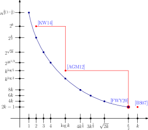
Graph sketching is a powerful technique introduced by the seminal work of Ahn, Guha and McGregor’12 on connectivity in dynamic graph streams that has enjoyed considerable attention in the literature since then, and has led to near optimal dynamic streaming algorithms for many fundamental problems such as connectivity, cut and spectral sparsifiers and matchings. Interestingly, however, the sketching and dynamic streaming complexity of approximating the shortest path metric of a graph is still far from well-understood. Besides a direct $k$-pass implementation of classical spanner constructions (recently improved to $\lfloor\frac{k}{2}\rfloor+1$-passes by Fernandez, Woodruff and Yasuda’20) the state of the art amounts to a $O(\log k)$-pass algorithm of Ahn, Guha and McGregor’12, and a $2$-pass algorithm of Kapralov and Woodruff’14. In particular, no single pass algorithm is known, and the optimal tradeoff between the number of passes, stretch and space complexity is open.

In this paper we introduce several new graph sketching techniques for approximating the shortest path metric of the input graph. We give the first single pass sketching algorithm for constructing graph spanners: we show how to obtain a $\widetilde{O}(n^{\frac{2}{3}})$-spanner using $\widetilde{O}(n)$ space, and in general a $\widetilde{O}(n^{\frac{2}{3}(1-\alpha)})$-spanner using $\widetilde{O}(n^{1+\alpha})$ space for every $\alpha\in[0,1]$, a tradeoff that we think may be close optimal. We also give new spanner construction algorithms for any number of passes, simultaneously improving upon all prior work on this problem. Finally, we note that unlike the original sketching approach of Ahn, Guha and McGregor’12, none of the existing spanner constructions yield simultaneous communication protocols with low per player information. We give the first such protocols for the spanner problem that use a small number of rounds.

1 Introduction

Graph sketching, introduced by [AGM12a] in an influential work on graph connectivity in dynamic streams has been a de facto standard approach to constructing algorithms for dynamic streams, where the algorithm must use a small amount of space to process a stream that contains both edge insertions and deletions. The main idea of [AGM12a] is to represent the input graph by its edge incident matrix, and applying classical linear sketching primitives to the columns of this matrix. This approach seamlessly extends to dynamic streams, as by linearity of the sketch one can simply subtract the updates for deleted edges from the summary being maintained: a surprising additional benefit is the fact that such a sketching solution is trivially parallelizable: since the sketch acts on the columns of the edge incidence matrix, the neighborhood of every vertex in the input graph is compressed independently. In particular, this yields efficient protocols in the simultaneous communication model, where every vertex knows its list of neighbors, and must communicate a small number of bits about this neighborhood to a coordinator, who then announces the answer. Surprisingly, several fundamental problems such as connectivity [AGM12a], cut [AGM12c] and spectral sparsification [AGM13, KLM⁺14, KMM⁺20] admit sketch based simultaneous communication protocols with only polylogarithmic communication overhead per vertex, which essentially matches existentially optimal bounds. The situation is entirely different for the problem of approximating the shortest path metric of the input graph: it is not known whether existentially best possible space vs approximation quality tradeoffs can be achieved using a linear sketch. This motivates the main question that we study:

What are the optimal space/stretch/pass tradeoffs for approximating the shortest path metric using a linear sketch?

Sketching and dynamic streams.

Sketching is the most popular tool for designing algorithms for the dynamic streaming model. Sketching solutions have been recently constructed for many graph problems, including spanning forest computation [AGM12b], cut and spectral sparsifiers [AGM13, KLM⁺14, KMM⁺20], spanner construction [AGM12c, KW14], matching and matching size approximation [AKLY16, AKL17], sketching the Laplacian [ACK⁺16, JS18] and many other problems. Also, results showing universality of sketching for this application are known, at least under some restrictions on the stream. The result of [LNW14] shows such an equivalence under the assumption that the stream length is at least doubly exponential in the size of the graph. The assumption on the stream length was significantly relaxed for binary sketches, i.e., sketches over $\mathbb{GF}_{2}$, by [HLY19, KMSY18]. Very recently, it has been shown [KP20] that lower bounds on stream length are crucial for such universality results: the authors of [KP20] exhibit a problem with a sketching complexity, which is polynomial in the input size, that can be solved in polylogarithmic space on a short dynamic stream.

Spanners in the sketching model.

A subgraph $H=(V,E)$ of a graph $G=(V,E)$ is a $t$-spanner of $G$ if for every pair $u,v\in V$ one has

$$d_{G}(u,v)\leq d_{H}(u,v)\leq t\cdot d_{G}(u,v)~{},$$

where $d_{G}$ stands for the shortest path metric of $G$ and $d_{H}$ for the shortest path metric of $H$. We assume in this paper that the input graph is unweighted, as one can reduce to this case using standard techniques at the expense of a small loss in space complexity. For every integer $k\geq 1$, every graph $G=(V,E)$ with $n$ vertices admits a $(2k-1)$-spanner with $O(n^{1+1/k})$ edges, which is optimal assuming the Erdős girth conjecture. The greedy spanner [ADD⁺93, FS20], which is sequential by nature, obtain the optimal number of edges. The celebrated algorithm of Baswana and Sen [BS07] obtains $(2k-1)$-spanner with $\widetilde{O}(n^{1+1/k})$ edges. This algorithm consists of a sequence of $k$ clustering steps, and as observed by [AGM12c], can be implemented in $k$ passes over the stream using the existentially optimal $\widetilde{O}(n^{1+1/k})$ space. A central question is therefore whether it is possible to achieve the existentially optimal tradeoff using fewer rounds of communication, and if not, what the optimal space vs stretch tradeoff is for a given number of round of communication. Prior to our work this problem was studied in [AGM12c] and [KW14]. The former showed how to construct a $(k^{\log_{2}5}-1)$-spanner in $\log_{2}k$ passes using space $\widetilde{O}(n^{1+1/k})$, and the latter showed how to construct a $(2^{k}-1)$-spanner in two passes and $\widetilde{O}(n^{1+1/k})$ space. In a single pass, the previously best known algorithm which uses $n^{1+o(1)}$ space is simply to construct a spanning tree, guaranteeing distortion $n-1$. Thus, our first question is:

In a single pass in the dynamic semi streaming model using $\widetilde{O}(n)$ space, is it possible to construct an $o(n)$ spanner?

We prove the following theorem in Section 4, as a corollary we obtain a positive answer to the question above (as spectral sparsifier can be computed in a single dynamic stream pass [KLM⁺14]).

Theorem 1.

Let $G=(V,E)$ be an undirected, unweighted graph. For a parameter $\epsilon\in(0,\frac{1}{18}]$, suppose that $H$ is a $(1\pm\epsilon)$-spectral sparsifier of $G$. Then $\widehat{H}$ is an $\tilde{O}(n^{\frac{2}{3}})$-spanner of $G$, where $\widehat{H}$ is unweighted version of $H$.

Corollary 1.

There exists an algorithm that for any $n$-vertex unweighted graph $G$, the edges of which arrive in a dynamic stream, using $\tilde{O}(n)$ space, constructs a spanner with $O(n)$ edges and stretch $\widetilde{O}(n^{\frac{2}{3}})$ with high probability.

Additionally, for the same setting, using similar techniques, we prove stretch $\widetilde{O}(\sqrt{m})$ (see Theorem 7).

One might think that the polynomial stretch is suboptimal, but we conjecture that this is close to best possible, and provide a candidate hard instance for a lower bound in Appendix A. Specifically,

Conjecture 1.

Any linear sketch from which one can recover an $n^{2/3-\Omega(1)}$-spanner with probability at least $0.9$ requires $n^{1+\Omega(1)}$ space.

More generally, we give the following trade off between stretch and space in a single pass:

Corollary 2.

Consider an $n$-vertex unweighted graph $G$, the edges of which arrive in a dynamic stream. For every parameter $\alpha\in(0,1)$, there is an algorithm using $\widetilde{O}(n^{1+\alpha})$ space, constructs a spanner with stretch $\widetilde{O}(n^{\frac{2}{3}(1-\alpha)})$ with high probability.

Similarly, for the same setting, we prove stretch $\widetilde{O}(\sqrt{m}\cdot n^{-\alpha})$ (see Theorem 9).

Next, we consider the case when we are allowed to take more than one pass over the stream and ask the following question:

For positive integers $k$ and $s$, what is the minimal $f_{n}(k,s)$ such that an $f_{n}(k,s)$-stretch spanner can be constructed using $s$ passes over a dynamic stream of updates to the input $n$-vertex graph using $\tilde{O}(n^{1+\frac{1}{k}})$ space?

We present two results, which together improve upon all prior work on the problem. At a high level both results are based on the idea of repeatedly contracting low diameter subgraphs and running a recursive spanner construction on the resulting supergraph. The main idea of the analysis is to carefully balance two effects: (a) loss in stretch due to the contraction process and (b) the reduction in the number of nodes in the supergraph. Since the number of nodes in the supergraphs obtained through the contraction process is reduced, we can afford to construct better spanners on them and still fit within the original stretch budget. A careful balancing of these two phenomena gives our results. Our first result uses a construction based on a clustering primitive implicit in [KW14] (see Lemma 6) and gives the best known tradeoff in at most $\log k$ passes:

Theorem 2.

For every real $k\in[1,\log n]$, and integer $g\in[1,\log k]$, there is a $g+1$ pass dynamic stream algorithm that given an unweighted, undirected $n$-vertex graph $G=(V,E)$, uses $\tilde{O}(n^{1+\frac{1}{k}})$ space, and computes w.h.p. a spanner $H$ with $\tilde{O}(n^{1+\frac{1}{k}})$ edges and stretch $2\cdot(2^{\left\lceil(\frac{k+1}{2})^{\nicefrac{{1}}{{g}}}\right\rceil}-1)^{g}-1<2^{g\cdot k^{\nicefrac{{1}}{{g}}}}\cdot 2^{g+1}$.

Using the same algorithm, while replacing the aforementioned clustering primitive from Lemma 6 with a clustering primitive from [BS07] (see Lemma 7), we obtain the following result, which provides the best known tradeoff for more than $\log_{k}$ passes:

Theorem 3.

For every real $k\in[1,\log n]$, and integer $g\in[1,\log k]$, there is a $g\cdot\left(\left\lceil(\frac{k+1}{2})^{\nicefrac{{1}}{{g}}}\right\rceil-1\right)+1<g\cdot k^{\nicefrac{{1}}{{g}}}+1$ pass dynamic stream algorithm that given an unweighted, undirected $n$-vertex graph $G=(V,E)$, uses $\tilde{O}(n^{1+\frac{1}{k}})$ space, and computes w.h.p. a spanner $H$ with $\tilde{O}(n^{1+\frac{1}{k}})$ edges and stretch $2\cdot\left(2\cdot\left\lceil(\frac{k+1}{2})^{\nicefrac{{1}}{{g}}}\right\rceil-1\right)^{g}-1\approx 2^{g}\cdot\left(k+1\right)$.

The proofs of Theorem 2 and Theorem 3 are presented in Section 6. We present our improvements over prior work in Table 1 below, where the results of Theorem 2 and Theorem 3 are present via several corollaries, presented in Section 6.3.

#Passes	Space	Stretch	Reference
$1$	$\tilde{O}(n)$	$\tilde{O}(n^{\nicefrac{{2}}{{3}}})$	Corollary 1
$1$	$\tilde{O}(n^{1+\frac{1}{k}})$	$\tilde{O}(n^{\nicefrac{{2}}{{3}}(1-\frac{1}{k})})$	Corollary 2
$2$	$\tilde{O}(n^{1+\nicefrac{{1}}{{k}}})$	$2^{k}-1$	[KW14]
$2$	$\tilde{O}(n^{1+\nicefrac{{1}}{{k}}})$	$2^{\frac{k+3}{2}}-3$	Corollary 5
$g+1$	$\tilde{O}(n^{1+\nicefrac{{1}}{{k}}})$	$2^{g\cdot k^{\nicefrac{{1}}{{g}}}}\cdot 2^{g+1}$	Theorem 2
$\log k$	$\tilde{O}(n^{1+\nicefrac{{1}}{{k}}})$	$k^{\log 5}-1$	[AGM12c]
$\log(k+1)$	$\tilde{O}(n^{1+\nicefrac{{1}}{{k}}})$	$2\cdot k^{\log 3}-1$	Corollary 7
$g\cdot k^{\nicefrac{{1}}{{g}}}+1$	$\tilde{O}(n^{1+\nicefrac{{1}}{{k}}})$	$\approx 2^{g}\cdot\left(k+1\right)$	Theorem 3
$k$	$\tilde{O}(n^{1+\nicefrac{{1}}{{k}}})$	$2k-1$	[BS07]
$\lfloor\frac{k}{2}\rfloor+1$	$\tilde{O}(n^{1+\nicefrac{{1}}{{k}}})$	$2k-1$	Corollary 6, [FWY20]

Figure 1: Trade-offs of various algorithms between stretch to number of passes. On the left summery of previous and current results. In Theorem 2 and Theorem 3 $g$ can be chosen to be any integer in $[1,\log k]$. On the right in blue is a plot of the results in this paper, while the previous results depicted in red. All the results are for algorithms using $\tilde{O}(n^{1+\frac{1}{k}})$ space. The $Y$ axis represents the stretch, while the $X$ axis is the number of passes. Some second order terms are neglected.

Simultaneous communication model.

We also consider the related simultaneous communication model, which we now define. In the simultaneous communication model every vertex of the input graph $G=(V,E),|V|=n,$ knows its list of neighbors (so that every $e=(u,v)\in E$ is known to both $u$ and $v$), and all vertices have a source of shared randomness. Communication proceeds in rounds, where in every round the players simultaneously post short messages on a common board for everyone to see (note that equivalently, one could consider a coordinator who receives all the messages in a given round, and then posts a message of unbounded length on the board). Note that a given player’s message in any given round may only depend on their input and other players’ messages in previous rounds. The content of the board at the end of the communication protocol must reveal the answer with high constant probability. The cost of a protocol in the simultaneous communication model is the length of the longest message communicated by any player.

Sketching algorithms for dynamic connectivity and cut/spectral approximations based on the idea of applying a sketch to the edge incidence matrix of the input graph [AGM12a, KLM⁺14, KMM⁺20] immediately yield efficient single pass simultaneous communication protocols with only polylogarithmic message length. We note, however, that existing sketch based algorithms for spanner construction (except for our result in Corollary 1 and the trivial $k$-pass implementation of the algorithm of Baswana and Sen [BS07]) do not yield low communication protocols. This is because they achieve reductions in the number of rounds by performing some form of leader election and amortizing communication over all vertices. See Remark 6 in Appendix D for more details. To illustrate the difference between dynamic streaming and simultaneous communication model, consider the following artificial problem. Suppose that we are given a graph with all but $\sqrt{n}$ isolated vertices, and the task is to recover the induced subgraph. Then using sparse recovery we can recover all the edges between the vertices using a single pass over a dynamic stream of updates. However, it is clear from information theoretic considerations that a typical vertex will need to communicate $\Omega(\sqrt{n})$ bits of information to solve this problem.

The main result of Section 5.1 is the following theorem.

Theorem 4.

For any integer $g\geq 1$, there is an algorithm (see Algorithm 1) that in $g$ rounds of communication outputs a spanner with stretch $\min\left\{\tilde{O}(n^{\frac{g+1}{2g+1}}),~{}(12+o(1))\cdot n^{2/g}\cdot\log n\right\}$.

Note that when $g=1$, the above theorem gives a $\widetilde{O}(n^{2/3})$ approximation using polylogarithmic communication per vertex. We think that the $n^{2/3}$ approximation is likely best possible in polylogarithmic communication per vertex, and the same candidate hard instance from Appendix A that we propose for 1 can probably be used to obtain a matching lower bound. Analyzing the instance appears challenging due to the fact that every edge is shared by the two players – exactly the feature of our model that underlies our algorithmic results (this sharing is crucial for both connectivity and spectral approximation via sketches). This model bears some resemblance to the number-on-the-forehead (NOF) model in communication complexity (see, for example, [KMPV19], where a connection of this form was made formal, resulting in conditional hardness results for subgraph counting in data streams).

The proof of this theorem is presented in Section 5.1.

Additionally, in Section 5.2 we first provide a trade off between size of the communication per player and stretch in one round of communication.

Theorem 5.

There is an algorithm that in $1$ round of communication, where each player communicates $\tilde{O}(n^{\alpha})$ bits, outputs a spanner with stretch

$$\min\left\{\widetilde{O}(n^{(1-\alpha)\frac{2}{3}}),~{}\widetilde{O}\left(\sqrt{m}\cdot n^{-\alpha}\right)\right\}~{}.$$

Then, we also prove a similar trade off when more than one round of communication is allowed.

Theorem 6.

For any integer $g\geq 1$, there is an algorithm that in $g$ rounds of communication, where each player communicates $\tilde{O}(n^{\alpha})$ bits, outputs a spanner with stretch

$$\min\left\{(12+o(1))\cdot n^{(1-\alpha)\cdot\frac{2}{g}}\cdot\log n~{},~{}\widetilde{O}\left(n^{\frac{(g+1)(1-\alpha)}{2g+1}}\right)\right\}~{}.$$

Parallel work.

Very recently, in a paper about the message-passing model, Fernandez et al. [FWY20] implemented Baswana-Sen [BS07] algorithm in $\lfloor\frac{k}{2}\rfloor+1$ passes in the semi-streaming model. This is the same as our Corollary 6 (which follows from Theorem 3 by setting $g=1$). While writing this paper, the authors were not aware of [FWY20] result.

The idea of recursively constructing a spanner by contracting clusters, which is the main idea leading to our Theorems 2 and 3, was found and used concurrently and independently from us by Biswas et al. [BDG⁺20] in the context of the massive parallel computation (MPC) model.

Related work.

Streaming algorithms are well-studied with too many results to list and we refer the reader to [McG14, McG17] for a survey of streaming algorithms. The idea of linear graph sketching was introduced in a seminal paper of Ahn, Guha, and McGregror [AGM12b]. An extension of the sketching approach to hypergraphs were presented in [GMT15]. The simultaneous communication model has also been used for lower bounding the performance of sketching algorithms – see, e.g.  [AKLY16, KKP18].

Spanners are a fundamental combinatorial object. They have been extensively studied and have found numerous algorithmic applications. We refer to the survey [ABS⁺20] for an overview. The most relevant related work is on insertion only streams [Elk11, Bas08] where the focus is on minimizing the processing time of the stream, and dynamic algorithms, where the goal is to efficiently maintain a spanner while edges are continuously inserted and deleted [Elk11, BKS12, BFH19].

2 Preliminaries

All the logarithms in the paper are in base $2$. We use $\tilde{O}$ notation to suppress constants and poly-logarithmic factors in $n$, that is $\widetilde{O}(f)=f\cdot{\rm polylog}(n)$.

We consider undirected, graphs $G=(V,E)$, with a weight function $w:E\to\mathbb{R}_{\geq 0}$. If we say that a graph is unweighted, we mean that all the edges have unit weight. $\widehat{G}=(V,E,\mathbbm{1}_{E})$ denotes the unweighted version of $G$, i.e. the graph $G$ where all edge weights are changed to $1$. Sometimes we abuse notation and write $G$ instead of $E$. Given two subsets $X,Y\subseteq V$, $E_{G}(X,Y)$ is the set of edges from $X$ to $Y$, $w_{G}(X,Y)$ denotes the total weight of edges in $E_{G}(X,Y)$ (number if $G$ is unweighted). We sometimes abuse notation and write instead $E_{G}(X\times Y)$ and $w_{G}(X\times Y)$ (respectively). For a subset of vertices $A\subseteq V$, let $G[A]$ denote the induced graph on $A$.

Let $d_{G}$ denote the shortest path metric in $G$. A subgraph $H$ of $G$ is a $t$-spanner of $G$ if for every $u,v\in V$, $d_{H}(u,v)\leq t\cdot d_{G}(u,v)$ (note that as $H$ is a subgraph of $G$, necessarily $d_{G}(u,v)\leq d_{H}(u,v)$). Following the triangle inequality, in order to prove that $H$ is a $t$-spanner of $G$ it is enough to show that for every edge $(u,v)\in E$, $d_{H}(u,v)\leq t\cdot d_{G}(u,v)$.

For an unweighted graph $G=(V,E)$, such that $|V|=n$ and $|E|=m$, let $B_{G}\in\mathbb{R}^{m\times n}$ denote the vertex edge incidence matrix. The Laplacian matrix of $G$ is defined as $L_{G}:=B_{G}^{\top}B_{G}$. Similarly, for a weighted graph $H=(V,E,w)$, we let $W\in\mathbb{R}^{m\times m}$ be the diagonal matrix of the edge weights. The Laplacian of the graph $H$ is defined as $L_{H}:=B_{H}^{\top}WB_{H}$. $H\preceq G$ denotes that for every $\vec{x}\in\mathbb{R}^{n}$, $\vec{x}^{t}L_{H}\vec{x}\leq\vec{x}^{t}L_{G}\vec{x}$. We say that a graph $H$ is $(1\pm\epsilon)$-spectral sparsifier of a graph $G$, if

$$(1-\epsilon)H\preceq G\preceq(1+\epsilon)H~{}.$$

Fact 1.

Suppose that a graph $H$ is a $(1\pm\epsilon)$-spectral sparsifier of a graph $G$, then $H$ is a $(1\pm\epsilon)$-cut sparsifier of $G$, i.e., for every set of vertices $S\subset V$, we have

$$(1-\epsilon)\cdot w_{H}(S,V\setminus S)~{}\leq~{}w_{G}(S,V\setminus S)~{}\leq~{}(1+\epsilon)\cdot w_{G}(S,V\setminus S)~{}.$$

For any Laplacian matrix $L_{G}$, we denote its Moore-Penrose pseudoinverse by $L_{G}^{+}$. For any pair of vertices $u,v\in V$, we denote their indicator vector by $b_{uv}=\chi_{u}-\chi_{v}$, where $\chi_{u}\in\mathbb{R}^{n}$ is the indicator vector of $u$, i.e., the entry corresponding to $u$ is $+1$ and all other entries are zero. Also, for any edge $e=(u,v)$, we define its indicator vector as $b_{e}:=b_{uv}$. We also define effective resistance of a pair of vertices $u,v\in V$ as

$$R_{uv}^{G}:=b_{uv}^{\top}L^{+}_{G}b_{uv}.$$

Fact 2.

Given a $(1\pm\epsilon)$-spectral sparsifier $H$ of a $G$, for every $u,v\in V$ it holds that

$$(1-\epsilon)R_{uv}^{G}~{}\leq~{}R_{uv}^{H}~{}\leq~{}(1+\epsilon)R_{uv}^{G}.$$

The following fact is a standard fact about effective resistances (see e.g., [SS08])

Fact 3.

In every $n$ vertex graph $G=(V,E,w)$ it holds that $\sum_{e\in E}w_{e}R_{e}^{G}~{}\leq~{}n-1$.

Dynamic streams.

In dynamic streams, there is a fixed set $V$ of $n$ vertices, unweighted edges arrive in a streaming fashion, where they are both inserted and deleted.

$\ell_{0}$-samplers.: Given integer vector in $\mathbb{R}^{n}$ in a dynamic stream, using $s\cdot{\rm polylog}(n)$ space, we can sample $s$ different non-zero entries. In particular if the vector is $s$-sparse, we can reconstruct it. Furthermore, given a stream of edges in an $n$-vertex graph $G$, using $s\cdot{\rm polylog}(n)$ samplers per vertex, we can create a subgraph $\tilde{G}$ of $H$ where each vertex has either at least $s$ edges, or has all its incident edges from $G$. This samplers are linear, therefore if we sum up the samplers of $S$ vertices, we can sample an outgoing edge.

Consider a vector $\vec{v}\in\mathbb{R}^{n}$, given a subset $A\subseteq[n]$ of coordinates, we denote by $\vec{v}[A]$ the restriction of $\vec{v}$ to $A$.

Lemma 1.

Consider a vector $\vec{v}\in\mathbb{R}^{n}$ that arrives in a dynamic stream via coordinate updates. The coordinates $[n]$ are partitioned into subsets $A_{1},A_{2},\dots,A_{r}$ (the space required to represent this partition is negligible). Let $\mathcal{I}=\left\{i\mid\vec{v}[A_{i}]\neq\vec{0}\right\}$ be the indices of the coordinate sets on which $\vec{v}$ is not zero. Given $A_{1},A_{2},\ldots,A_{r}$ and a parameter $s>0$, and a guarantee that $\left|\mathcal{I}\right|\leq s$, using $s\cdot{\rm polylog}(n)$ space, one can design a sketching algorithm recovering a set $S\subseteq[n]$ such that

• For every $j\in S$, $\vec{v}_{j}\neq 0$.

• For every $i\in\mathcal{I}$, $A_{i}\cap S\neq\emptyset$.

The proof uses a technique commonly used in sketching literature, and is given in Section B.1 for completeness.

Lemma 2.

[Edge recovery] Consider an unweighted, undirected graph $G=(V,E)$ that is received in a dynamic stream. Given $A,B\subseteq V$ such that $A\cap B=\emptyset$, one can design a sketching algorithm that using ${\rm polylog}(n)$ space in a single pass over the stream, with probability $1/{\rm poly}(n)$, can either recover an edge between $A$ to $B$, or declare that there is no such edge.
Further, provided that there are at most $m$ edges in $A\times B$, using $m\cdot{\rm polylog}(n)$ space, with probability $1/{\rm poly}(n)$ we can recover them all.

The proof is using the same techniques as in the proof of Lemma 1 and is deferred to Section B.1.

3 Technical Overview

We consider an $n$ vertex unweighted graph $G=(V,E)$.

Spectral sparsifiers are spanners (Section 4).

The technical part of the paper begins by proving the following fact: consider a spectral sparsifier $H$ of $G$. Consider an edge $(u,v)\in E$. Denote the distance between its endpoints in $\widehat{H}$ by $d_{\widehat{H}}(u,v)=s$. Divide the vertices $V$ into the BFS layers w.r.t. $u$ in $\widehat{H}$. That is, $A_{i}$ is the set of all vertices at distance $i$ from $u$ in $\widehat{H}$. In particular $v\in A_{s}$. See illustration on the right. Let $W_{i}^{G}=w_{G}(A_{i}\times A_{i+1})$ be the total weight of the edges in $E_{G}(A_{i},A_{i+1})$. Similarly $W_{i}^{H}=w_{H}(A_{i}\times A_{i+1})$. Let $H^{\prime}$ be the graph created from $H$ by contracting all the vertices in each set $A_{i}$ into a single vertex. The rough intuition is the following:

$$1\overset{(a)}{\geq}R_{u,v}^{G}\overset{(b)}{\gtrsim}R_{u,v}^{H}\overset{(c)}{\geq}R_{u,v}^{H^{\prime}}\overset{(d)}{=}\sum_{i=0}^{s-1}\frac{1}{W_{i}^{H}}\overset{(*)}{\approx}\sum_{i=0}^{s-1}\frac{1}{W_{i}^{G}}\overset{(e)}{\geq}\sum_{i=0}^{s-1}\frac{1}{|A_{i}||A_{i+1}|}\overset{(f)}{\geq}\Omega\left(\frac{s^{3}}{n^{2}}\right)~{}.$$ (3.1)

Here (a) follows as the effective resistance between the endpoints of an edge is at most $1$. (b) as $H$ is a spectral sparsifier of $G$. (c) as the effective resistance can only reduce by contracting vertices. (d) as $H^{\prime}$ is a path graph. (e) as $G$ is unweighted and thus $W_{i}^{G}$ is bounded by the number of edges in $A_{i}\times A_{i+1}$. And (f) as $\sum_{i}|A_{i}|\leq n$ and the function $\sum_{i=0}^{s-1}\frac{1}{|A_{i}||A_{i+1}|}$ is minimized when $|A_{i}|=\Omega(\frac{n}{s})$ for all $i$. The tricky part is the rough equality (*). Note that if Equation 3.1 holds, it will follow that $s=O(n^{\frac{2}{3}})$, implying the desired stretch.

While $H$ is a spectral sparsifier of $G$, $W_{i}^{G}$ does not represent the size of a cut in $G$. This is as there might be edges in $G$ crossing from $A_{i}$ to $\cup_{j>i+1}A_{j}$, or from $A_{i+1}$ to $\cup_{j<i}A_{j}$. Thus a priori there is no reason to expect that $W_{i}^{H}$ will approximate $W_{i}^{G}$. Interestingly, we were able to show that $W_{i}^{G}=W_{i}^{H}\pm\epsilon\cdot(W_{i-1}^{H}+W_{i}^{H}+W_{i+1}^{H})$. That is, while we are not able to bound $|W_{i}^{G}-W_{i}^{H}|$ using the standard factor $\epsilon\cdot W_{i}^{H}$, we can bound this error once we take into account also the former and later cuts in the BFS order! We use this fact to show that for most of the indices $i$, $W_{i}^{H}\leq|A_{i}||A_{i+1}|$. The desired bound follows. See proof of Theorem 1 for more details.

Next, using similar analysis we show that in case where the graph $G$ has $m$ edges, the stretch of $\widehat{H}$ is bounded by $O(\sqrt{m})$ (see Theorem 7). Suppose that $d_{\widehat{H}}(u,v)=s$. Intuitively, following Equation 3.1, as $\sum_{i}W_{i}^{G}\leq m$, it follows that $1\geq R_{u,v}^{G}\gtrsim\sum_{i=0}^{s-1}\frac{1}{W_{i}^{G}}=\Omega\left(\frac{s^{2}}{m}\right)$ (as $\sum_{i=0}^{s-1}\frac{1}{W_{i}^{G}}$ us minimized when all $W_{i}^{G}$’s are equal), implying $s=O(\sqrt{m})$. Both bounds ($O(n^{\frac{2}{3}})$ and $O(\sqrt{m})$) are tight. Essentially, we construct the exact instance tightening all the inequalities in Equation 3.1. That is a graph with $\widetilde{\Theta}(n^{\frac{2}{3}})$ layers, each one containing $\widetilde{\Theta}(n^{\frac{1}{3}})$ vertices, and all possible edges between layers (see Section 4.2).

In Section 4.3, we show that using $\widetilde{O}(n^{1+\alpha})$ space (instead of $\widetilde{O}(n)$), the stretch can be reduced to

$$\min\{\widetilde{O}(n^{\frac{2}{3}(1-\alpha)}),\widetilde{O}(\sqrt{m}\cdot n^{-\alpha})\}.$$

The idea is the following: randomly partition the graph $G$ into $\widetilde{O}(n^{2\alpha})$ induced subgraphs $G_{1},G_{2},\dots$, such that each $G_{i}$ contains $O(n^{1-\alpha})$ vertices, and every pair of vertices $u,v$ belong to some $G_{i}$. Furthermore, the (expected) number of edges in each $G_{i}$ is $m\cdot n^{-2\alpha}$. Next, we construct a spectral sparsifier for each graph $G_{i}$ and take their union as our spanner. The stretch gurantee follows (see Theorem 8, Corollary 2 and Theorem 9).

Simultaneous communication model (Section 5).

In a single pass, one can construct a spectral sparsifier and therefore obtain the exact same results as in the streaming model. However, as opposed to streaming, no known approach can reduce the stretch in less than logarithmic number of rounds. We propose a natural peeling algorithm (see Algorithm 1). Denote $G_{1}=G$. Given a desired stretch parameter $t$, the algorithm computes a spectral sparsifier $H_{1}$, and removes all the satisfied edges $(u,v)\in E$ where $d_{\widehat{H}_{1}}(u,v)\leq t$, to obtain a graph $G_{2}$. Generally, in the $i$’th round the algorithm computes a spectral sparsifier $H_{i}$ for the graph $G_{i}$, and removes all the satisfied edges to obtain $G_{i+1}$. This procedure continues until all the edges are satisfied (that is $G_{i+1}=\emptyset$). The resulting spanner is $\widehat{H}=\cup_{i}\widehat{H}_{i}$ the union of (the unweighted version of) all the constructed sparsifiers. Notably, for every parameter $t\geq 1$ the algorithm will eventually halt, and return a $t$-spanner. The arising question is, how many rounds are required to satisfy a specific parameter $t$?

We show that this procedure will halt after $g$ steps for

$$t\geq\min\{\tilde{O}(n^{\frac{g+1}{2g+1}})~{},~{}(12+o(1))\cdot n^{2/g}\cdot\log n\}$$

(see Theorem 4). Interestingly, in $g=\log n$ rounds we can obtain stretch $O(\log n)$, which is asymptotically optimal. That is, we present a completely new construction for a $O(\log n)$-spanner with $\tilde{O}(n)$ edges. Interestingly, there are constructions of spectral sparsifiers which are based on taking a union of poly-logarithmically many $O(\log n)$-stretch spanners (see [KP12, KX16]). In a sense, here we obtain the opposite direction. That is, by taking a union of $\log n$ sparsifiers, one can construct an $O(\log n)$ stretch spanner. That is, sparsifiers and spanners are much more related from what one may initially expect.

To show that the algorithm halts in $g$ round for a specific $t$, we bound the number of edges in $G_{i}$, which eventually will lead us to conclusion that $G_{g+1}=\emptyset$:

• Set $t=\tilde{O}(n^{\frac{g+1}{2g+1}})$. Here the analysis is based on the effective resistance. Using Equation 3.1, one can see that after the first round, $G_{2}$ will contain only edges with effective resistance at least $\Omega(\frac{t^{3}}{n^{2}})$ (in $G$). As the sum of all effective resistances is bounded by $n-1$, we conclude $|G_{2}|\leq\Omega(\frac{n^{3}}{t^{3}})$. In general, following the $O(\sqrt{m})$ upper bound on stretch, one can show that $G_{i+1}$ contain only edges with effective resistance $\Omega(\frac{t^{2}}{|G_{i}|})$, implying $|G_{i+1}|\leq\frac{n}{t^{2}}|G_{i}|$. $t$ is chosen so that $|G_{g}|\leq t^{2}$, hence a spectral sparsifier will have stretch at most $\sqrt{|G_{g}|}=t$ for all the edge, implying $G_{g+1}=\emptyset$.

• Set $t=O(n^{2/g}\cdot\log n)$. Here the analysis is based on low diameter decomposition. In general, for a weighted graph $H$ and parameter $\phi=n^{-2/g}$, we construct a partition $\mathcal{C}$ of the vertices, such that each cluster $C\in\mathcal{C}$ has hop-diameter $O(\frac{\log n}{\phi})=t$ (i.e. w.r.t. $\widehat{H}$), and the overall fraction of the weight of inter-cluster edges is bounded by $\phi$. Following our peeling algorithm, when this clustering is preformed w.r.t. $H_{i}$, $G_{i+1}$ will contain only inter-cluster edges from $G_{i}$. As $H_{i}$ is a spectral sparsifier of $G_{i}$, the size of all cuts are preserved. It follows that $|G_{i+1}|\lesssim\phi\cdot|G_{i}|$. In particular, in $\log_{\frac{1}{\phi}}|G|\leq g$ rounds, no edges will remain.
  Interestingly, for this analysis to go through it is enough that each $H_{i}$ will be a cut sparsifier of $G_{i}$, rather than a spectral sparsifier. Oppositely, a single cut sparsifier $H$ of $G$ can have stretch $\tilde{\Omega}(n)$ (see Remark 1).

Next, similarly to the streaming case, we show that if each player can communicate a message of size $\widetilde{O}(n^{\alpha})$ in each round, then we can construct a spanner with stretch $\min\{\widetilde{O}(n^{\frac{2}{3}(1-\alpha)}),\widetilde{O}(\sqrt{m}\cdot n^{-\alpha})\}$ in a single round, or stretch $\min\left\{(12+o(1))\cdot n^{(1-\alpha)\cdot\frac{2}{g}}\cdot\log n~{},~{}\widetilde{O}\left(n^{\frac{(g+1)(1-\alpha)}{2g+1}}\right)\right\}$ in $g$ rounds (see Theorem 5 and Theorem 6). The approach is the same as in the streaming case, and for the most part, the analysis follows the same lines. However, the single round $\widetilde{O}(\sqrt{m}\cdot n^{-\alpha})$ bound is somewhat more involved. Specifically, in the streaming version we’ve made the assumption that $m\leq n^{1+\alpha}$, as otherwise, using sparse recovery we can restore the entire graph. Unfortunately, sparse recovery is impossible here. Instead, we show that in a single communication round we can partition the vertex set $V$ into $V_{1},V_{2}$, such that all the incident edges of $V_{1}$ are restored, while the minimum degree in $G[V_{2}]$ is at least $n^{\alpha}$. The rest of the analysis goes through.

Pass-stretch trade-off (Section 6).

Fix the allowed space of the algorithm to be $\widetilde{O}(n^{1+\frac{1}{k}})$. Both [BS07] and [KW14] algorithms are based on clustering. Specifically, they have $k$ clustering phases, where in the $i$’th phase there are about $n^{1-\frac{i}{k}}$ clusters. Eventually, after $k-1$ phases the number of clusters is $n^{\frac{1}{k}}$, and an edge from every vertex to every cluster could be added to the spanner. In [BS07], each clustering phase takes a single dynamic stream pass, while the diameter of each $i$-level cluster is bounded by $2i$. On the other hand, in [KW14] all the clusters are constructed in a single dynamic stream pass, while the diameter of each $i$-level clusters is only bounded by $2^{i+1}-2$.

Our basic approach is the following: execute either [BS07] or [KW14] clustering procedure for some $i$ steps. Then, construct a super graph $\mathcal{G}$ by contracting each cluster into a single vertex, and (recursively) compute a spanner $\mathcal{H}$ for the super graph $\mathcal{G}$ with stretch $k^{\prime}<k$. Eventually, for each super edge in $\mathcal{H}$, we will add a representative edge into the resulting spanner $H$. The basic insight, is that while the usage of a cluster graph instead of the actual graph increases the stretch by a multiplicative factor of the clusters diameter, we are able to compute a spanner with stretch $k^{\prime}$ considerably smaller than $k$, and thus somewhat compensating for the loss in the stretch.

This phenomena has opposite effects when applying it on either [BS07] or [KW14] clustering schemes. Specifically, applying this idea on [BS07] for $g$ recursive steps, we will obtain stretch $2^{g}\cdot k$ (compared with $2k-1$ in [BS07]) while reducing the number of passes to $g\cdot k^{\nicefrac{{1}}{{g}}}$ (compared with $k$ in [BS07]). That is we get a polynomial reduction in the number of passes, while paying a constant increase in stretch. From the other hand, applying this idea on [KW14] for $g$ recursive steps, we will obtain stretch $2^{g\cdot k^{\nicefrac{{1}}{{g}}}}$ (compared to $2^{k}-1$ in [KW14]) while reducing the number of passes to $g+1$ (compared with $2$ in [KW14]). Thus for each additional pass, we get an exponential reduction in the stretch.

Interestingly, the idea of recursively constructing a spanner by contracting clusters was found and used concurrently and independently from us by Biswas et al. [BDG⁺20] in the context of the massive parallel computation (MPC) model. They applied it only on [BS07] algorithm in order to construct a spanner in small number of rounds.

4 Spectral Sparsifiers are Spanners

In this section, we show that spectral sparsifiers can be used to achieve low stretch spanners in one pass over the stream. Our algorithm works as follows: first, given a graph $G=(V,E)$, it generates a (possibly weighted) spectral sparsifier $H$ of $G$, using the sketches which can be stored in $\tilde{O}(n)$ space [KLM⁺14, KNST19, KMM⁺20]. Then, the weights of all edges are set to be equal to $1$. We show that the resulting graph $\widehat{H}$ is a $\tilde{O}(n^{\frac{2}{3}})$-spanner of the original graph.

See 1

As [KLM⁺14] constructed $(1\pm\epsilon)$-spectral sparsifier with $O(\frac{n}{\epsilon^{2}})$ edges in a dynamic stream, by fixing $\epsilon=\frac{1}{18}$, we conclude: See 1

Proof of Theorem 1.

By triangle inequality, it is enough to prove that for every edges $(u,v)\in E$, it holds that $d_{\widehat{H}}(u,v)=\tilde{O}(n^{\frac{2}{3}})$. Our proof strategy is as follows: consider a pair of vertices $u,v\in V$ such that $d_{\widehat{H}}(u,v)=s$. We will prove that $R_{u,v}^{G}\geq\tilde{\Omega}(\frac{s^{3}}{n^{2}})$. As for every pair of neighboring vertices it holds that $R_{u,v}^{G}\leq 1$, the theorem will follow.

Consider a pair of vertices $v,u\in V$ such that $d_{\widehat{H}}(v,u)=s$. We partition $V$ to sets $A_{0},A_{1},\dots,A_{s}$ where for $i<s$, $A_{i}=\{z\in V\mid d_{\widehat{H}}(v,z)=i\}$ are all the vertices at distance $i$ from $v$ in $\widehat{H}$. $A_{s}=\{z\in V\mid d_{\widehat{H}}(v,z)\geq s\}$ are all the vertices at distance at least $s$. Let $W_{i}^{H}=w_{H}(A_{i}\times A_{i+1})$ be the total weight in $H$ (the weighted sparsifier) of all the edges between $A_{i}$ to $A_{i+1}$. Similarly, set $W_{i}^{G}=w_{G}(A_{i}\times A_{i+1})$. We somewhat abused notation here, we treat non-existing edges as having weight $0$, while all the edges in the unweighted graph $G$ have unit weight. For simplicity of notation set also $W_{-1}^{H}=W_{-1}^{G}=W_{s}^{H}=W_{s}^{G}=0$. Note that while $W_{i}^{H}$ denotes the size if a cut in $H$, it does not correspond to a cut in $G$ (as e.g. there might be edges from $A_{i}$ to $A_{i+2}$). Thus, a priori there should not be a resemblance between $W_{i}^{G}$ to $W_{i}^{H}$. Nevertheless, we show that $W_{i}^{H}$ approximates $W_{i}^{G}$. However, the approximation will depend also on $W_{i-1}^{H},W_{i+1}^{H}$ rather than only on $W_{i}^{H}$.

Claim 1.

For every $i$, $W_{i}^{H}-\epsilon\cdot(W_{i-1}^{H}+W_{i}^{H}+W_{i+1}^{H})\leq W_{i}^{G}\leq W_{i}^{H}+\epsilon\cdot(W_{i-1}^{H}+W_{i}^{H}+W_{i+1}^{H})$.

Proof of 1.

For a fixed $i$, set

$$\begin{array}[]{ll}A_{<i}=A_{0}\cup\dots\cup A_{i-1}&A_{>i+1}=A_{i+2}\cup\dots\cup A_{s}\\ A_{\leq i}=A_{0}\cup\dots\cup A_{i}&A_{\geq i+1}=A_{i+1}\cup\dots\cup A_{s}\end{array}$$

In addition we denote the weight of several edge sets as follows, (see Figure 2 for illustration)

$$\begin{array}[]{lll}a=w_{G}(A_{i}\times A_{i+1})&b=w_{G}(A_{i}\times A_{>i+1})&c=w_{G}(A_{<i}\times A_{i+1})\\ d=w_{G}(A_{<i}\times A_{>i+1})&e=w_{G}(A_{<i}\times A_{i})&f=w_{G}(A_{i+1}\times A_{>i+1})\end{array}$$ (4.1)

Figure 2: An illustration of the diffferent edges sets, the weight of which is denoted in Equation 4.1. Note that $a=W_{i}^{G}$, $e=W_{i-1}^{G}$, and $f=W_{i+1}^{G}$.

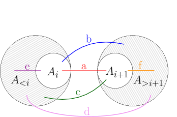
Similarly by replacing $w_{G}$ with $w_{H}$ in Equation 4.1, we obtain the values $a^{\prime},b^{\prime},c^{\prime},d^{\prime},e^{\prime},f^{\prime}$ (e.g. $a^{\prime}=w_{H}(A_{i}\times A_{i+1})$). Note that by the definition of the sets $A_{0},\dots,A_{s}$, it holds that $b^{\prime}=c^{\prime}=d^{\prime}=0$. Using this notation, 1 states that $a^{\prime}-\epsilon\cdot(a^{\prime}+e^{\prime}+f^{\prime})\leq a\leq a^{\prime}+\epsilon\cdot(a^{\prime}+e^{\prime}+f^{\prime})$.

Note that any $(1\pm\epsilon)$-spectral sparsifier is a $(1\pm\epsilon)$-cut sparsifier. Thus, as $H$ is a $(1\pm\epsilon)$-spectral sparsifier of $G$, it preserves weights of all the cuts up to $\epsilon$ error factors. We derive the following inequalities: $(1-\epsilon)a^{\prime}$ $\leq$ $a+b+c+d$ $\leq$ $(1+\epsilon)a^{\prime}$ By $(A_{\leq i},A_{\geq i+1})$-cut $(1-\epsilon)f^{\prime}$ $\leq$ $b+d+f$ $\leq$ $(1+\epsilon)f^{\prime}$ By $(A_{\leq i+1},A_{>i+1})$-cut $(1-\epsilon)e^{\prime}$ $\leq$ $c+d+e$ $\leq$ $(1+\epsilon)e^{\prime}$ By $(A_{<i},A_{\geq i})$-cut $(1-\epsilon)(a^{\prime}+e^{\prime}+f^{\prime})$ $\leq$ $a+d+e+f$ $\leq$ $(1+\epsilon)(a^{\prime}+e^{\prime}+f^{\prime})$ By $(A_{<i}\cup A_{i+1},A_{i}\cup A_{>i+1})$-cut

Or equivalently

$$\begin{array}[]{ccccc}(1-\epsilon)a^{\prime}&\leq&a+b+c+d&\leq&(1+\epsilon)a^{\prime}\\ -(1+\epsilon)f^{\prime}&\leq&-b-d-f&\leq&-(1-\epsilon)f^{\prime}\\ -(1+\epsilon)e^{\prime}&\leq&-c-d-e&\leq&-(1-\epsilon)e^{\prime}\\ (1-\epsilon)(a^{\prime}+e^{\prime}+f^{\prime})&\leq&a+d+e+f&\leq&(1+\epsilon)(a^{\prime}+e^{\prime}+f^{\prime})\end{array}$$

By summing up these 4 inequalities, and dividing by $2$, we get

$$a^{\prime}-\epsilon\cdot(a^{\prime}+e^{\prime}+f^{\prime})\leq a\leq a^{\prime}+\epsilon\cdot(a^{\prime}+e^{\prime}+f^{\prime})~{}.$$

The claim now follows. ∎

Our next goal is to bound $\sum_{i=0}^{s-1}\frac{1}{W_{i}^{H}}$, as this quantity lower-bounds the resistance between $u$ and $v$ in $H$. Since $\sum_{i=0}^{s}|A_{i}|=n$ and $W_{i}^{G}\leq|A_{i}|\cdot|A_{i+1}|$, one can bound $\sum_{i=0}^{s-1}\frac{1}{W_{i}^{G}}$ by $\Omega\left(\frac{s^{3}}{n^{2}}\right)$. However relating this quantity to the effective resistances in $G$ is not as straightforward as one might expect.

Claim 2.

$\sum_{i=0}^{s-1}\frac{1}{W_{i}^{H}}\geq\Omega\left(\frac{s^{3}}{n^{2}}\cdot\frac{\log^{2}\frac{1}{\epsilon}}{\log^{2}n}\right)$.

Proof of 2.

For all $i\in[s]$, set $a_{i}=|A_{i}|$. Set

$$\alpha:=10\log_{\frac{1}{6\epsilon}}n^{2}~{},$$ (4.2)

and

$$I:=\left\{i\in[s]\mid a_{i}\leq\frac{\alpha n}{s}\right\}.$$

It holds that $|I|\geq\left(1-\frac{1}{\alpha}\right)s+1$, as otherwise there are at least $\frac{s}{\alpha}$ indices $i$ for which $a_{i}>\frac{\alpha n}{s}$, implying $\sum_{i}a_{i}>n$, a contradiction, since $A_{0},\dots,A_{s}$ forms a partition of $V$. Set

$$\widetilde{I}:=\left\{i\mid\text{such that }\forall j~{}\text{such that }|i-j|\leq\frac{\alpha}{10},~{}\text{ it holds that }j\in I\right\}.$$

Note that, since there are less than $\frac{s}{\alpha}$ indices $i$ such that $i\notin I$, then there are less than $\frac{s}{\alpha}\cdot\frac{2\alpha}{10}\leq\frac{s}{5}$ indices out of $\widetilde{I}$, implying

$$\left|\widetilde{I}\right|\geq\frac{s}{2}~{}.$$ (4.3)

Fix an index $i_{0}\in\widetilde{I}$, we argue that $W_{i_{0}}^{H}\leq 2\left(\frac{\alpha n}{s}\right)^{2}$. For every index $j\in\left[i_{0}-\frac{\alpha}{10},i_{0}+\frac{\alpha}{10}-1\right]$, it holds that $W_{j}^{G}=|E_{G}(A_{j},A_{j+1})|\leq a_{j}\cdot a_{j+1}\leq\left(\frac{\alpha n}{s}\right)^{2}$. Assume for the sake of contradiction that $W_{i_{0}}^{H}>2\left(\frac{\alpha n}{s}\right)^{2}$. We prove by induction that for $1\leq j\leq\frac{\alpha}{10}$, there is an index $i_{j}$ such that $|i_{j}-i_{0}|\leq j$ and $W_{i_{j}}^{H}>\frac{1}{(6\epsilon)^{j}}\left(\frac{\alpha n}{s}\right)^{2}$. For the base case, by 1,

$$W_{i_{0}-1}^{H}+W_{i_{0}}^{H}+W_{i_{0}+1}^{H}\geq\frac{1}{\epsilon}\left(W_{i_{0}}^{H}-W_{i_{0}}^{G}\right)>\frac{1}{\epsilon}\left(2\left(\frac{\alpha n}{s}\right)^{2}-\left(\frac{\alpha n}{s}\right)^{2}\right)=\frac{1}{\epsilon}\left(\frac{\alpha n}{s}\right)^{2}~{}.$$

The we can choose $i_{1}\in\left\{i_{0}-1,i_{0},i_{0}+1\right\}$ such that $W_{i_{1}}^{H}>\frac{1}{3\epsilon}\left(\frac{\alpha n}{s}\right)^{2}>\frac{1}{6\epsilon}\left(\frac{\alpha n}{s}\right)^{2}$.
For the induction step, suppose that there is an index $i_{j}$ such that $|i_{j}-i_{0}|\leq j<\frac{\alpha}{10}$ and ${W_{i_{j}}^{H}>\frac{1}{(6\epsilon)^{j}}\left(\frac{\alpha n}{s}\right)^{2}}$. As $|i_{j}-i_{0}|\leq\frac{\alpha}{10}-1$, it follows that $W_{i_{j}}^{G}\leq\left(\frac{\alpha n}{s}\right)^{2}$. Hence

$$W_{i_{j}-1}^{H}+W_{i_{j}}^{H}+W_{i_{j}+1}^{H}\geq\frac{1}{\epsilon}\left(W_{i_{j}}^{H}-W_{i_{j}}^{G}\right)\geq\frac{1}{\epsilon}\left(\frac{1}{(6\epsilon)^{j}}\left(\frac{\alpha n}{s}\right)^{2}-\left(\frac{\alpha n}{s}\right)^{2}\right)>\frac{1}{2\epsilon}\cdot\frac{1}{(6\epsilon)^{j}}\left(\frac{\alpha n}{s}\right)^{2}~{}.$$

Thus there is an index $i_{j+1}\in\left\{i_{j}-1,i_{j},i_{j}+1\right\}$ such that $W_{i_{j+1}}^{H}>\frac{1}{(6\epsilon)^{j+1}}\left(\frac{\alpha n}{s}\right)^{2}$, as required.

We conclude that,

$$W_{i_{\frac{\alpha}{10}}}^{H} ~{}>~{}\left(6\epsilon\right)^{-\frac{\alpha}{10}}\left(\frac{\alpha n}{s}\right)^{2}~{}\overset{(\ref{eq:alpha})}{\geq}~{}n^{2}\left(\frac{\alpha n}{s}\right)^{2}~{}\geq~{}n^{2}~{},$$

where the last inequality follows as $s\leq n$. This is a contradiction, as $H$ is an $(1\pm\epsilon)$ spectral sparsifier of the unweighted graph $G$, where the maximal size of a cut is $\frac{n^{2}}{4}$. We conclude that for every $i\in\widetilde{I}$, it holds that $W_{i}^{H}\leq 2\left(\frac{\alpha n}{s}\right)^{2}$. The claim now follows as

$$\sum_{i=0}^{s-1}\frac{1}{W_{i}^{H}} \geq\left|\widetilde{I}\right|\cdot\frac{1}{2}\left(\frac{\alpha n}{s}\right)^{-2}$$

$$\geq\frac{s^{3}}{4\alpha^{2}n^{2}}$$ By Equation 4.3

$$=\Omega\left(\frac{s^{3}}{n^{2}}\cdot\frac{\log^{2}\frac{1}{\epsilon}}{\log^{2}n}\right)$$ By Equation 4.2 (4.4)

∎

We are now ready to prove the theorem. Construct an auxiliary graph $H^{\prime}$ from $H$, by contracting all the vertices inside each set $A_{i}$, and keeping multiple edges. Note that by this operation, the effective resistance between $u$ and $v$ cannot increase. The graph $H^{\prime}$ is a path graph consisting of $s$ vertices, where the conductance between the $i$’th vertex to the $i+1$’th is $W_{i}^{H}$. Using 2, we conclude

$$(1+\epsilon)R_{u,v}^{G} \geq R_{u,v}^{H}$$ By 2

$$\geq R_{u,v}^{H^{\prime}}$$ As explained above

$$=\sum_{i=0}^{s-1}\frac{1}{W_{i}^{H}} H^{\prime}$$ Since is a path graph

$$=\Omega\left(\frac{s^{3}}{n^{2}}\cdot\frac{\log^{2}\frac{1}{\epsilon}}{\log^{2}n}\right)~{}$$ By Equation 4.4 (4.5)

As $u,v$ are neighbors in the unweighted graph $G$, it necessarily holds that $R_{u,v}^{G}\leq 1$, implying that $s=O\left(\left(n^{2}\cdot\frac{\log^{2}n}{\log^{2}\frac{1}{\epsilon}}\right)^{\frac{1}{3}}\right)=\widetilde{O}\left(n^{\frac{2}{3}}\right)$. ∎

We state the following corollary, based on the last part of the proof of Theorem 1.

Corollary 3.

Let $G=(V,E)$ be an unweighted undirected graph, and let $H$ be a $(1\pm\epsilon)$-spectral sparsifier of $G$ for some small enough constant $\epsilon$. Also, let $\widehat{H}$ denote the unweighted $H$. If for a pair of vertices $u,v\in V$ we have $s:=d_{\widehat{H}}(u,v)$, then

$$R_{u,v}^{G}=\widetilde{\Omega}\left(\frac{s^{3}}{n^{2}}\right),$$

and

$$R_{u,v}^{H}=\widetilde{\Omega}\left(\frac{s^{3}}{n^{2}}\right).$$

4.1 Sparse graphs

Suppose we are guaranteed that the graph $G$ we receive in the dynamic stream has eventually at most $m$ edges. In Theorem 7 we show that the distortion guarantee of a sparsifier is at most $\widetilde{O}(\sqrt{m})$, and thus together with Theorem 1 it is $\widetilde{O}(\min\{\sqrt{m},n^{\nicefrac{{2}}{{3}}}\})$. Later, in Section 5 we will use this to obtain a two pass algorithm in the simultaneous communication model with distortion $\widetilde{O}(n^{\nicefrac{{3}}{{5}}})$.

Theorem 7.

Let $G=(V,E)$ be an undirected, unweighted such that $|V|=n$ and $|E|=m$. For a parameter $\epsilon\in(0,\frac{1}{18}]$, suppose that $H$ is a $(1\pm\epsilon)$-spectral sparsifier of $G$. Then $\widehat{H}$ is an $\widetilde{O}(\sqrt{m})$-spanner of $G$, where $\widehat{H}$ is the unweighted version of $H$.

The proof follows similar lines to the proof of Theorem 1 and is deferred to Section B.2. Theorem 7 implies a streaming algorithm using space $\tilde{O}(n)$ that constructs a spanner with stretch $\tilde{O}(\sqrt{m})$. Notice that the number of edges $m$, does not need to be known in advance.

Similar to Corollary 3, using the last part of the proof of Theorem 7, we conclude the following:

Corollary 4.

Let $G=(V,E)$ be an unweighted undirected graph with $m=|E|$, and let $H$ be a $(1\pm\epsilon)$-spectral sparsifier of $G$ for some small enough constant $\epsilon$. Also, let $\widehat{H}$ denote the unweighted $H$. If for a pair of vertices $u,v\in V$ we have $s:=d_{\widehat{H}}(u,v)$, then

$$R_{u,v}^{G}=\widetilde{\Omega}\left(\frac{s^{2}}{m}\right),$$

and

$$R_{u,v}^{H}=\widetilde{\Omega}\left(\frac{s^{2}}{m}\right).$$

4.2 Tightness of Theorem 1 and Theorem 7

In this section, we show that the stretch guarantees in Theorem 1 and Theorem 7 are tight up to polylogarithmic factors.

Lemma 3 (Tightness of Theorem 1).

For every large enough $n$, there exists an unweighted $n$ vertex graph $G$, and a spectral sparsifier $H$ of $G$ such that $\widehat{H}$ has stretch $\widetilde{\Omega}(n^{2/3})$ w.r.t. $G$.

Proof.

As was shown by Spielman and Srivastava [SS08], one can create a sparsifier $H$ of $G$ (with high probability) by adding each edge $e$ of $G$ to $H$ with probability $p_{e}=\min\{\epsilon^{-2}\cdot R_{e}^{G}\cdot\log n,1\}$ (and weight $1/p_{e}$). This approach is known as spectral sparsification using effective resistance sampling. We will construct a graph $G$ and argue that for a random graph $H$ sampled according to the scheme above [SS08], the stretch of $\widehat{H}$ will (likely) be $\widetilde{\Omega}(n^{2/3})$.

For brevity, we will construct a graph with $n+2$ vertices and ignore rounding issues. The graph $G=(V,E)$ is constructed as follows. Let $N:=\frac{n^{\nicefrac{{2}}{{3}}}}{c}$ for $c:=\log n$. We partition the set of vertices, $V$, into $V_{0},V_{1},\ldots,V_{N},V_{N+1}$, where for each $i\in[1,N]$, we have $|V_{i}|=a=cn^{\nicefrac{{1}}{{3}}}$, and $V_{0}=\{u\}$, $V_{N+1}=\{v\}$ are singletons. For every $i\in[0,N]$, we connect all vertices in $V_{i}$ to all vertices in $V_{i+1}$, and furthermore, we connect $u$ and $v$ by an edge called $e$. That is,

$$E=\left(\cup_{i=0}^{N}V_{i}\times V_{i+1}\right)\cup\{(u,v)\}.$$

Figure 3: An illustration of the graph $G$ constructed during the proof of Lemma 3.

See Figure 3 for illustration. Next, we calculate $R_{e}^{G}$, by observing the flow vector when one units of flow is injected in $v$ and is removed from $u$. Denote $R:=R_{e}^{G}$. Then $R$ units of flow is routed using edge $e$, while $(1-R)$ units of flow is routed using the rest of the graph. By symmetry, for each cut $V_{i}\times V_{i+1}$ the flow will spread equally among the edges. Farther, the potential of all the vertices in each set $V_{i}$ is equal. Denote by $P_{i}$ the potential of vertices in $V_{i}$. Thus $0=P_{0}<P_{1}<\dots<P_{N+1}=R$. For $i=0$, each edge in $V_{0}\times V_{1}$ carries $\frac{(1-R)}{a}$ flow, thus $P_{1}-P_{0}=\frac{(1-R)}{a}$. Similarly, $P_{N+1}-P_{N}=\frac{(1-R)}{a}$. On the other hand, for $i\in[1,N-1]$, each edge in $V_{i+1}\times V_{i}$ carries $\frac{(1-R)}{a^{2}}$ flow, thus $P_{i+1}-P_{i}=\frac{(1-R)}{a^{2}}$. We conclude

$$R=P_{N+1}-P_{0}=\sum_{i=0}^{N}(P_{i+1}-P_{i})=2\cdot\frac{(1-R)}{a}+\frac{(1-R)}{a^{2}}\cdot(N-1)=(1-R)\cdot\frac{2a+|N|-1}{a^{2}}$$

Thus,

$$R_{e}^{G}=R=\frac{2a+|N|-1}{a^{2}-2a-|N|+1}=\frac{2cn^{\nicefrac{{1}}{{3}}}+\frac{n^{\nicefrac{{2}}{{3}}}}{c}-1}{c^{2}n^{\nicefrac{{2}}{{3}}}-2cn^{\nicefrac{{1}}{{3}}}-\frac{n^{\nicefrac{{2}}{{3}}}}{c}+1}=\frac{1}{c^{3}}(1+o(1))=O(\frac{1}{\log^{3}n})~{}.$$

Note that it is thus most likely that $e$ will not belong to $H$ (for large enough $n$). For a sampled graph $H$ excluding $e$, we will have $d_{\widehat{H}}(u,v)\geq|N|=\widetilde{\Omega}(n^{2/3})$. From the other hand, as a graph $H$ sampled in this manner is a spectral sparsifier with high probability, it implies the existence of a spectral sparsifier $H$ of $G$ with stretch $\widetilde{\Omega}(n^{2/3})$, as required. ∎

Lemma 4 (Tightness of Theorem 7).

For every large enough $m$, there exists an unweighted graph $G$ with $m$ edges, and a spectral sparsifier $H$ of $G$ such that $\widehat{H}$ has stretch $\widetilde{\Omega}(\sqrt{m})$ w.r.t. $G$.

Proof.

Fix $n=(\frac{m}{2\log m})^{\nicefrac{{3}}{{4}}}$. Note that the graph we constructed during the proof of Lemma 3 has $2a+(N-1)a^{2}=2cn^{\nicefrac{{1}}{{3}}}+(\frac{n^{\nicefrac{{2}}{{3}}}}{c}-1)\cdot c^{2}n^{\nicefrac{{2}}{{3}}}<2c\cdot n^{\nicefrac{{4}}{{3}}}<m$ edges. We can complement it to exactly $m$ edges by adding some isolated component. Following Lemma 3, this graph has a sparsifier $H$, such that $\widehat{H}$ has stretch $\widetilde{\Omega}(n^{2/3})=\widetilde{\Omega}(\sqrt{m})$ w.r.t. $G$, as required.

∎

Remark 1.

Cut sparsifiers are somewhat weaker version of spectral sparsifiers. Specifically, a weighted subgraph $H$ of $G$ is called a cut sparsifier if it preserves the size of all cuts (up to $1\pm\epsilon$ factor). A natural question is the following: given a cut sparsifier $H$ of $G$, how good of a spanner is $\widehat{H}$?
The answer is: very bad. Specifically, consider the hard instance constructed during the proof of Lemma 3. Construct the same graph $G$ where we change the parameter $N$ to equal $\Theta(\frac{n}{\log n})$ and $a$ to $\Theta(\log n)$. There exist a cut sparsifier $H$ of $G$ excluding the edge $e=(u,v)$. In particular, $\widehat{H}$ will have stretch $\widetilde{\Omega}(n)$.

4.3 Stretch-Space trade-off

In this section, we first prove a result, which given an algorithm that uses $\widetilde{O}(n)$ space in the dynamic streaming setting, converts it to an algorithm that uses $\widetilde{O}(n^{1+\alpha})$ space and achieves a better stretch guarantee (see Theorem 8). Then, we apply this theorem to Corollary 1 and get a space-stretch trade off. Next, in Theorem 9 we prove a similar trade off in terms of number of edges.

Theorem 8.

Assume there is an algorithm, called Alg, that given a graph $G=(V,E)$ in a dynamic stream, with $|V|=n$, using $\widetilde{O}(n)$ space, outputs a spanner with stretch $\widetilde{O}(n^{\beta})$ for some constant $\beta\in(0,1)$ with failure probability $n^{-c}$ for some constant $c$. Then, for any constant $\alpha\in(0,1)$, one can construct an algorithm that uses $\widetilde{O}(n^{1+\alpha})$ space and outputs a spanner with stretch $\widetilde{O}(n^{\beta(1-\alpha)})$ with failure probability $\tilde{O}(n^{(2+c)\alpha-c})$.

Proof.

Let $\mathcal{P}\subset 2^{[n]}$ be a set of subsets of $[n]$ such that: (1) $|\mathcal{P}|=O(n^{2\alpha}\log n)$, (2) every $P\in\mathcal{P}$ is of size $|P|=O(n^{1-\alpha})$, and (3) for every $i,j\in[n]$ there is a set $P\in\mathcal{P}$ containing both $i,j$. Such a collection $\mathcal{P}$ can be constructed by a random sampling. Denote $V=\{v_{1},\dots,v_{n}\}$. For each $P\in\mathcal{P}$, set $A_{P}=\{v_{i}\mid i\in P\}$. For each $P\in\mathcal{P}$, we use Alg independently to construct a spanner $H_{P}$ for $G[A_{P}]$ the induced graph on $A_{P}$. The final spanner will be their union $H=\cup_{P\in\mathcal{P}}H_{P}$.

The space (and also the number of edges in $H$) used by our algorithm is bounded by $\sum_{P\in\mathcal{P}}\widetilde{O}(|P|)=\widetilde{O}(n^{2\alpha}\cdot n^{1-\alpha})=\widetilde{O}(n^{1+\alpha})$. From the other hand, for every $v_{i},v_{j}\in V$ such that $i,j\in P$, it holds that

$$d_{H}(v_{i},v_{j})\leq d_{H_{P}}(v_{i},v_{j})\leq\widetilde{O}(|P|^{\beta})\leq\widetilde{O}(n^{\beta(1-\alpha)})~{}.$$

By union bound, the failure probability is bounded by $\tilde{O}(n^{2\alpha})\cdot O(n^{-c(1-\alpha)})=\tilde{O}(n^{(2+c)\alpha-c})$.

∎

Combining Corollary 1 with Theorem 8, we conclude: See 2

Remark 2.

We can reduce the number of edges in the spanner returned to $O(n)$, by incurring additional $O(\log n)$ factor to the stretch. This is done by computing additional spanner upon the one returned by Corollary 2.

Following the approach in Theorem 8, we can also use more space to reduce the stretch parameterized by the number of edges. Note that the Theorem 9 provides better result than Corollary 2 when $m\leq n^{\frac{4}{3}+\frac{2}{3}\alpha}$.

Theorem 9.

Consider an $n$-vertex unweighted graph $G$, the edges of which arrive in a dynamic stream. For every parameter $\alpha\in(0,1)$, there is an algorithm using $\widetilde{O}(n^{1+\alpha})$ space, constructs a spanner with stretch $\widetilde{O}(\sqrt{m}\cdot n^{-\alpha})$.

Proof.

Similarly to Theorem 8, our goal here is to partition the vertices into $\approx n^{2\alpha}$ sets of similar size. However, while in Theorem 8 we wanted to bound the number of vertices in each set, here we want to bound the edges in each set. As the edge set is unknown, we cannot use a fixed partition. Rather, in the preprocessing phase we will sample a partition that w.h.p. will be good w.r.t. arbitrary fixed edge set.

Fix $p=n^{-\alpha}$. With no regard to the rest of the algorithm, during the stream we will sample $\widetilde{O}(n^{1+\alpha})=\widetilde{O}(\frac{n}{p})$ edges from the stream using sparse recovery (Lemma 2), and add them to our spanner $\widehat{H}$. If $m\leq np^{-1}$, we will restore the entire graph $G$, and thus will have stretch $1$. The rest of the analysis will be under the assumption that $m>np^{-1}$.

For every $i\in[1,\frac{8}{p^{2}}\ln n]$, sample a subset $A_{i}$ by adding each vertex with probability $p$. Consider a single subset $A_{i}$ sampled in this manner, and denote $G_{i}=G[A_{i}]$ the graph it induces. We will compute a sparsifier $H_{i}$ for $G_{i}$. Our final spanner will be $\widehat{H}=\cup_{i}\widehat{H}_{i}$ a union of the unweighted versions of all the sparsifiers (in addition to the random edges sampled above). The space we used for the algorithm is $\sum_{i}\widetilde{O}(|A_{i}|)$. Note that with high probability, by Chernoff inequality $\sum_{i}\widetilde{O}(|A_{i}|)=\widetilde{O}(n^{2\alpha}\cdot n^{1-\alpha})=\widetilde{O}(n^{1+\alpha})$.

Next we bound the stretch. Consider a pair of vertices $(u,v)\in E$. Denote by $\psi_{i}$ the event that both $u,v$ belong to $A_{i}$. Note that $\Pr[\psi_{i}]=p^{2}$. Denote by $m_{i}=\left|{A_{i}\choose 2}\cap E\right|$ the number of edges in $G_{i}$. Set

$$\mu_{i}=\mathbb{E}\left[m_{i}\mid\psi_{i}\right]\leq 1+p\cdot\left(\deg_{G}(v)+\deg_{G}(u)\right)+mp^{2}<1+2np+mp^{2}<4mp^{2}~{},$$

to be the expected number of edges in $G_{i}$ provided that $u,v\in A$. The first inequality follows as (1) $(u,v)\in G_{i}$, (2) every edge incident on $u,v$ belongs to $G_{i}$ with probability $p$, and (3) every other edge belongs to $G_{i}$ with probability $p^{2}$. In the final inequality we used the assumption $n<mp$. Denote by $\phi_{i}$ the event that $m_{i}\leq 8mp^{2}$. By Markov we have

$$\Pr\left[\psi_{i}\wedge\phi_{i}\right]=\Pr\left[\psi_{i}\right]\cdot\Pr\left[\phi_{i}\mid\psi_{i}\right]\geq\frac{1}{2}p^{2}~{}.$$

As $\{\psi_{i}\wedge\phi_{i}\}_{i}$ are independent, we have that the probability that none of them occur is bounded by

$$\Pr\left[\bigwedge_{i}\left(\overline{\psi_{i}\wedge\phi_{i}}\right)\right]\leq(1-\frac{1}{2}p^{2})^{\frac{8}{p^{2}}\ln n}<e^{-\frac{1}{2}p^{2}\cdot\frac{8}{p^{2}}\ln n}=n^{-4}~{}.$$

Note that if both $\psi_{i},\phi_{i}$ occurred, and $H_{i}$ is an $1\pm\epsilon$ sparsifier of $G_{i}$, by Theorem 1 we will have that

$$d_{\widehat{H}}(u,v)\leq d_{\widehat{H}_{i}}(u,v)\leq\widetilde{O}(\sqrt{m_{i}})=\widetilde{O}(\sqrt{m}\cdot p)=\widetilde{O}(\sqrt{m}\cdot n^{-\alpha})$$

By union bound, the probability that for every $(u,v)\in E$, there is some $i$ such that $\psi_{i}\wedge\phi_{i}$ occurred is at least $1-n^{-2}$. The probability that every $G_{i}$ is a spectral sparsifier is $1-n^{-\Omega(1)}$. The theorem follows by union bound.

∎

5 Simultaneous Communication Model

In Section 4, we considered streaming model and proved results for the setting when one pass over the stream was allowed. The remaining question is as follows: using small number of communication rounds (but more than $1$), can we improve the stretch of a spanner constructed in the simultaneous communication model? A partial answer is given in the following subsections.

First, in Section 5.1 we present a single filtering algorithm that provides two different trade-offs between stretch and number of communication rounds (see Algorithm 1 and Theorem 4). Basically, the algorithm receives a parameter $t>1$, in each communication round, an unweighted version of a sparsifier is added to the spanner. Then, locally in each vertex, all the edges that already have a small stretch in the current spanner are deleted (stop being considered), and another round of communication begins.

In Theorem 4 we present two arguments. The first argument is based on effective resistance filtering, which results in a spanner with $\tilde{O}(n^{\frac{g+1}{2g+1}})$ stretch in $g$ communication rounds. The second argument, which is based on low-diameter decomposition, results in a spanner with $\tilde{O}\left(n^{\frac{2}{g}}\right)$ stretch in $g$ communication rounds. The latter approach outputs a spanner with smaller stretch compared to the former algorithm for $g\geq 4$.

Finally, in Section 5.2 we generalize our results to the case where each player is allowed $\tilde{O}(n^{\alpha})$ communication per round for some $\alpha\in(0,1)$. In that section, we prove two results: (1) in Theorem 5 we give a space (communication per player) stretch trade off for one round of communication (2) in Theorem 6 we give a similar trade off for more than one round of communication.

5.1 The filtering algorithm

The algorithm will receive a stretch parameter $t$. During the execution of the algorithm, we will hold in each step a spanner $\widehat{H}$, and a subset of unsatisfied edges. As the algorithm proceeds, the spanner will grow, while the number of unsatisfied edges will decrease. Initially, we start with an empty spanner $\widehat{H}$, and the set of unsatisfied edges $E_{0}=E$ is the entire edge set. In general, at round $i$, we hold a set $E_{i}$ of edges yet unsatisfied. We construct a spectral sparsifier $H_{i}$ for the graph $G_{i}=(V,E_{i})$ over thus edges. $\widehat{H}_{i}$, the unweighted version of $H_{i}$ is added to the spanner $\widehat{H}$. $E_{i+1}$ is defined to be all the edges $(u,v)\in E_{i}$, for which the distance in $\widehat{H}$ is greater than $t$, that is $d_{\widehat{H}}(u,v)>t$. Note that as the sparsifier $H_{i}$, and hence the spanner $\widehat{H}$ is known to all, each vertex locally can compute which of its edges belong to $E_{i+1}$.

In addition, the algorithm will receive as an input parameter $g$ to bound the number of communication rounds. We denote by $E_{g+1}$ the set of unsatisfied edge by the end of the algorithm. That is edges from $(u,v)\in E$ for which $d_{\widehat{H}}(u,v)>t$. Note that during the execution of the algorithm, $E_{g+1}\subseteq E_{g}\subseteq E_{g-1}\subseteq\cdots\subseteq E_{1}=E$. Finally, if $E_{g+1}=\emptyset$, it will directly imply that $\widehat{H}$ is a $t$-spanner of $G$. See Algorithm 1 for illustration.

input : Graph $G=(V,E)$ (in simultaneous communication model), number of rounds $g$, stretch parameter $t$

output : $t$-spanner of $G$ with $\tilde{O}(n\cdot g)$ edges

1 $\epsilon\leftarrow\frac{1}{18}$

$\widehat{H}\leftarrow\emptyset$

  // $\widehat{H}$ will be the output spanner

2

3for $i=1$ to $g$ do

4       $E_{i}\leftarrow\{e=(u,v)\in G_{i-1}\text{ such that }d_{\widehat{H}}(u,v)>t\}$

5       $G_{i}\leftarrow(V,E_{i})$

6       Let $H_{i}$ be a $(1\pm\epsilon)$-spectral sparsifier of graph $G_{i}$.

       $\widehat{H}\leftarrow\widehat{H}\cup\widehat{H}_{i}$

        // $\widehat{H}_{i}$ is the unweighted version of $H_{i}$

7      

return $\widehat{H}$

Algorithm 1 Spanners Using Filtering$(G=(V,E),t,g)$

Below, we state the theorem, which proves the round complexity and correctness of Algorithm 1. See 4

Proof.

For $g=1$, the theorem holds due to Theorem 1, thus we will assume that $g\geq 2$. We prove each of the two upper-bounds on stretch separately. We prove the first bound using an effective resistance based argument. The latter upper-bound is proven using an argument based on filtering low-diameter clusters.

Effective resistance argument:

We execute Algorithm 1 with parameter $g$, and $t=\tilde{O}(n^{\frac{g+1}{2g+1}})$. Consider an edge $e=(u,v)\in E_{1}$. If $e\in E_{2}$, then it follows from Corollary 3 that $R_{u,v}^{H_{1}}=\tilde{\Omega}\left(\frac{t^{3}}{n^{2}}\right)$. Set $a_{1}=\tilde{\Omega}\left(\frac{t^{3}}{n^{2}}\right)$. Then

$$|E_{2}|\leq\frac{1}{a_{1}}\sum_{e\in E_{1}}R_{e}^{H_{1}}\leq\frac{1+\epsilon}{a_{1}}\sum_{e\in E_{i}}R_{e}^{G_{1}}\leq\frac{1+\epsilon}{a_{1}}\cdot(n-1)\leq\tilde{\Omega}\left(\frac{n^{3}}{t^{3}}\right)~{},$$ (5.1)

where the first inequality follows as $a_{1}\leq R_{e}^{H_{1}}$ for $e\in E_{2}$, the second inequality is by 2, and the third inequity follows by 3, as $G_{i-1}$ is unweighted. In general, for $i\geq 2$, we argue by induction that $|E_{i}|=\tilde{O}\left(\frac{n^{i+1}}{t^{2i-1}}\right)$. Indeed, consider an edge $e\in E_{i+1}$. Using the induction hypothesis, it follows from Corollary 4 that

$$R_{u,v}^{H_{i}}=\tilde{\Omega}\left(\frac{t^{2}}{|E_{i}|}\right)=\tilde{\Omega}\left(\frac{t^{2(i+1)-1}}{n^{i+1}}\right)$$

Set $a_{i}=\tilde{\Omega}\left(\frac{t^{2(i+1)-1}}{n^{i+1}}\right)$. Using the same arguments as in Equation 5.1, we get

$$|E_{i+1}|\leq\frac{1}{a_{i}}\sum_{e\in E_{i}}R_{e}^{H_{i}}\leq\frac{1+\epsilon}{a_{i}}\sum_{e\in E_{i}}R_{e}^{G_{i}}\leq\frac{1+\epsilon}{a_{i}}\cdot(n-1)\leq\tilde{O}\left(\frac{n^{(i+1)+1}}{t^{2(i+1)-1}}\right)~{}.$$

Finally, for every $e\in E_{g}$, following Theorem 7, it holds that

$$d_{\widehat{H}}(u,v)\leq d_{\widehat{H}_{g}}(u,v)\leq\tilde{O}\left(\sqrt{E_{g}}\right)=\tilde{\Omega}\left(\sqrt{\frac{n^{g+1}}{t^{2g-1}}}\right)\leq t~{},$$

where the last inequality holds for $t=\tilde{\Omega}(n^{\frac{g+1}{2g+1}})$. We conclude that $E_{g+1}=\emptyset$. The theorem follows.

Low diameter decomposition argument:

Fix $\phi=\frac{1}{3}n^{-\nicefrac{{2}}{{g}}}$. We will execute Algorithm 1 with parameter $g$ and $t=\frac{4+o(1)}{\phi}\cdot\ln n$. We argue that for every $i\in[2,g+1]$, $|E_{i+1}|\leq 3\phi|E_{i}|$. As $|E_{1}|<n^{2}$, it will follow that $E_{g+1}=\emptyset$, as required.

Consider the unweighted graph $G_{i}$, and the sparsifier $H_{i}$ we computed for it. We will cluster $G_{i}$ based on cut sizes in $H_{i}$. The clustering procedure is iterative, where in phase $j$ we holds an induced subgraph $H_{i,j}$ of $H_{i}$, create a cluster $C_{j}$, remove it from the graph $H_{i,j}$ to obtain an induced subgraph $H_{i,j+1}$, and continue. The procedure stops once all the vertices are clustered. Specifically, in phase $j$, we pick an arbitrary unclustered center vertex $v_{j}\in H_{i,j}$, and create a cluster by growing a ball around $v_{j}$. Set $B_{r}=B_{\hat{H}_{i,j}}(v_{j},r)$ to be the radius $r$ ball around $v_{j}$ in the unweighted version of $H_{i,j}$. That is $B_{r+1}=B_{r}\cup N(B_{r})$, where $N(B_{r})$ are the neighbors of $B_{r}$ in $H_{i,j}$. Let $r_{j}$ be the minimal index $r$ such that

$$\partial_{H_{i,j}}(B_{r})<\phi\cdot\mathrm{Vol}_{H_{i,j}}(B_{r})~{}.$$ (5.2)

Here $\partial_{H_{i,j}}(B_{r})$ denotes the total weight of the outgoing edges from $B_{r}$, while $\mathrm{Vol}_{\hat{H}_{i,j}}(B_{r})=\sum_{u\in B_{r}}\deg_{\hat{H}_{i,j}}(u)$ denotes the sum of the weighted degrees of all the vertices in $B_{r}$. Note that while $B_{r}$ is defined w.r.t. an unweighted graph $\widehat{H}_{i,j}$, $\partial_{H_{i,j}}$ and $\mathrm{Vol}_{H_{i,j}}$ are defined w.r.t. the weighted sparsifier. For every $r$, it holds that $\mathrm{Vol}_{\hat{H}_{i,j}}(B_{r+1})\geq\mathrm{Vol}_{\hat{H}_{i,j}}(B_{r})+\partial_{\hat{H}_{i,j}}(B_{r})$. We argue that $r_{j}\leq 2(1+\epsilon)\cdot{n\choose 2}$. If $v_{j}$ is isolated in $H_{i,j}$, then Equation 5.2 holds for $r=0$ and we are note. Else, as the minimal weight of an edge in a sparsifier is $1$, it holds that $\mathrm{Vol}_{H_{i,j}}(B_{0})=\deg_{H_{i,j}}(v_{j})\geq 1$. We conclude that for $r_{j}$, the minimal index for which Equation 5.2 holds, we have that

$$\mathrm{Vol}_{H_{i,j}}(B_{r_{j}})\geq(1+\phi)\mathrm{Vol}_{H_{i,j}}(B_{r-1})\geq\cdots\geq(1+\phi)^{r_{j}}\mathrm{Vol}_{H_{i,j}}(B_{0})\geq(1+\phi)^{r_{j}}~{},$$

On the other hand, as $H_{i}$ is a $(1+\epsilon)$ spectral sparsifier of an unweighted graph $G_{i}$, we have

$$\mathrm{Vol}_{H_{i,j}}(B_{r_{j}})\leq\mathrm{Vol}_{H_{i,j}}(H_{i,j})\leq 2(1+\epsilon)\cdot|E|\leq 2(1+\epsilon)\cdot{n\choose 2}~{}.$$

Therefore, it must holds that $(1+\phi)^{r_{j}}\leq 2(1+\epsilon){n\choose 2}$, which implies

$$r_{j}\leq\frac{\ln((1+\epsilon)n^{2})}{\ln(1+\phi)}=\frac{2+o(1)}{\phi}\cdot\ln n~{}.$$

We set $C_{j}=B_{r_{j}}$ and continue to construct $C_{j+1}$. Overall, we found a partition of the vertex set $V$ into clusters $C_{1},C_{2},\dots$ such that each cluster satisfies Equation 5.2, and has (unweighted) diameter at most $\frac{4+o(1)}{\phi}\cdot\ln n=t$. In particular, for every edge $e=(u,v)\in E_{i}$, if $u,v$ are clustered to the same $C_{i}$, then the distance between them in $\hat{H}$ will be bounded by $t$. Thus $E_{i+1}$ will be a subset $\partial_{H_{i}}(C_{1},C_{2},\ldots)$, the set of inter-cluster edges. It holds that

$$\partial_{H_{i}}(C_{1},C_{2},\ldots)=\sum_{j\geq 1}\partial_{H_{i,j}}(C_{j})\leq\phi\cdot\sum_{j\geq 1}\mathrm{Vol}_{H_{i,j}}(C_{j})\leq\phi\cdot\mathrm{Vol}_{H_{i}}(V)~{},$$ (5.3)

where the first inequality holds as each edge counted exactly once. For example the edge $(u,v)\in E(C_{a},C_{b})$, where $a<b$ counted only at $\partial_{\hat{H}_{i,a}}(C_{a})$. Hence,

$$|E_{i+1}|\leq\partial_{G_{i}}(C_{1},C_{2},\ldots) \leq(1+\epsilon)\partial_{H_{i}}(C_{1},C_{2},\ldots)$$ By 1

$$\leq(1+\epsilon)\phi\cdot\mathrm{Vol}_{H_{i}}(V)$$ By Equation 5.3

$$\leq\frac{\phi(1+\epsilon)}{1-\epsilon}\cdot\mathrm{Vol}_{G_{i}}(V)$$ By 1

$$=\phi\cdot\left(1+\frac{2\epsilon}{1-\epsilon}\right)\cdot 2|E_{i}|<3\phi\cdot|E_{i}|~{}.$$

∎

Remark 3.

Note that in fact for the low diameter decomposition argument, it is enough to use in Algorithm 1 cut sparsifiers rather than spectral sparsifiers.

5.2 Stretch-Communication trade-off

We note that if more communication per round is allowed, then we can obtain the following. See 5

Proof.

We prove the stretch bounds, one by one.

Proving $\widetilde{O}(n^{(1-\alpha)\frac{2}{3}})$:

Basically, the claim follows by Corollary 1. More specifically, we work on graphs induces on $O(n^{1-\alpha})$ sized set of vertices. For each such subgraph, we can construct sparsifiers using $O({\rm polylog}(n))$ sized sketches communicated by each vertex involved. Since each vertex is involved in $\widetilde{O}(n^{\alpha})$ subgraphs, then communication per vertex is $\widetilde{O}(n^{\alpha})$. And by Corollary 3, the stretch is $\widetilde{O}(n^{(1-\alpha)\frac{2}{3}})$.

Proving $\widetilde{O}\left(\sqrt{m}\cdot n^{-\alpha}\right)$:

First, the reader should note that we cannot directly use Corollary 4 for this part. The reason is that during the proof of Theorem 9, for the special case where $m\leq n^{1+\alpha}$, we simply used a sparse recovery procedure to recover the entire graph. However, as the graph $G$ might contain a dense subgraph, sparse recovery is impossible in the simultaneous communication model. Instead, we use a procedure, called peeling low degree vertices, where using $\widetilde{O}(n^{\alpha})$ bits of information per vertex, we can partition the vertices into two sets, $V_{1}$ and $V_{2}$, where all edges incident on $V_{1}$ are recovered and minimum degree in $G[V_{2}]$ is at least $n^{-\alpha}$. We present this procedure in Algorithm 2 and its guarantees are proved in Lemma 5 below.

Lemma 5 (Peeling low-degree vertices).

In a simultaneous communication model, where communication per player is $\tilde{O}(s)$, there is an algorithm that each vertex can locally run and output a partition of the vertices into $V_{1},V_{2}$ such that:

1. All the incident edges of $V_{1}$ are recovered.

2. The min-degree in the induce graph $G[V_{2}]$ is at least $s$.

Furthermore, the partitions output by all vertices are identical, due to the presence of shared randomness.

Proof.

First, we argue that using $s$-sparse recovery procedure on the neighborhood of vertices, one can find a set $V_{1}\subseteq V$ such that all the vertices in $V\setminus V_{1}$ have degree more than $s$. This is done in the following way: each vertex prepares an $s$-sparse recovery sketch for its neighborhood, and in the first round of communication writes its sketch alongside its degree on the board. Then, each vertex runs Algorithm 2 locally. Note that the output is identical in all vertices since they have access to shared randomness.

Now, we argue the correctness of Algorithm 2. First, we let Recover be a $s$-sparse recovery algorithm. More specifically, the following fact holds.

Fact 4.

For any integer $s$, given $S$, a $\widetilde{O}(s)$-bit sized linear $s$-sparse recovery sketch of a vector $\vec{b}$, such that $\textsc{Support}(\vec{b})\leq s$, algorithm $\textsc{Recover}(S)$ outputs the non-zero elements of $\vec{b}$, with high probability.

Consider the execution of Algorithm 2. If in the beginning there does not exist a low-degree vertex, we are done. Otherwise, there exists a vertex $u$ with degree $\leq s$. Now, when we call $\textsc{Recover}(S_{u})$ it is guaranteed that the support of the vector is bounded by $s$ (see Algorithm 2 of Algorithm 2). In that case, $\textsc{Recover}(S_{u})$ succeeds with high probability. Note that in case of success, the output of $\textsc{Recover}(S_{u})$ is deterministic- that is depend only the graph and not on the random coins. Then, we delete vertex $u$ alongside its incident edges. The sketches for the rest of the graph can be updated accordingly, since the sketches are linear. Thus, we can use the updated sketches in the next round to recover the neighborhood of another low-degree vertex (in the updated graph), without encountering dependency issues (as the series of events we should succeed upon is predetermined). We repeat this procedure until no vertex with degree $\leq s$ remains. Furthermore, we call Recover at most $n$ times per vertex (since we can delete at most $n$ vertices), in total, using union bound, the algorithm succeeds with high probability.

input : A parameter $s$, linear $s$-sparse recovery sketches (denoted by $S_{u}$ for each vertex $u$)

output : A partition of vertices into two sets, $V_{1}$ and $V_{2}$, with the guarantees mentioned in Lemma 5

1 $V_{1}\leftarrow\emptyset$

2 $V_{2}\leftarrow V$

3 while $\exists$ a vertex $u$ with degree $\leq s$ do

       $u\leftarrow$ a vertex with degree $\leq s$

        // Using a universal ordering, and degrees in $G[V_{2}]$

       $E_{u}\leftarrow\textsc{Recover}(S_{u})$

        // See 4

       Remove $E_{u}$ from the sketches and update degrees.

        // Sketches are linear

4       $V_{1}\leftarrow V_{1}\cup\{u\}$.

5       $V_{2}\leftarrow V_{2}\setminus\{u\}$.

return $(V_{1},V_{2})$

Algorithm 2 Low-Degree Peeling$(\{S_{u}\}_{u\in V},s)$

∎

We use Algorithm 2 with $s=n^{\alpha}$. In the same time, we use the algorithm from Theorem 9. That is, partition the vertices into $\widetilde{O}(n^{2\alpha})$ sets such that each vertex belong to each set with probability $n^{-\alpha}$. Than compute a sparsifier $H$ for each set and take their union. It follows that the total required communication is $\widetilde{O}(n^{\alpha})$ per vertex. Note that the algorithm of Theorem 9 is linear. Hence after using Lemma 5, we can add all the edges incident on $V_{1}$ to the spanner, and update the algorithm from Theorem 9 accordingly. That is we will use it only on $G[V_{2}]$.

Note that we have $|E(G[V_{2}])|\geq|V_{2}|\cdot n^{\alpha}$, and consequently we can use the argument in the proof of Theorem 9. In total from one hand we will obtain stretch $1$ on edges incident to $V_{1}$, and from the other hand, for edges inside $G[V_{2}]$ we will have stretch of $\widetilde{O}(\sqrt{|E(G[V_{2}])|}\cdot n^{\alpha})\leq\widetilde{O}(\sqrt{m}\cdot n^{\alpha})$. ∎ See 6

Proof.

We use the same set of subsets of vertices as in Theorem 8, i.e., let $\mathcal{P}\subset 2^{[n]}$ be a set of subsets of $[n]$ such that: (1) $|\mathcal{P}|=O(n^{2\alpha}\log n)$, (2) every $P\in\mathcal{P}$ is of size $|P|=O(n^{1-\alpha})$, and (3) for every $i,j\in[n]$ there is a set $P\in\mathcal{P}$ containing both $i,j$. Such a collection $\mathcal{P}$ can be constructed by a random sampling. Denote $V=\{v_{1},\dots,v_{n}\}$. For each $P\in\mathcal{P}$, set $A_{P}=\{v_{i}\mid i\in P\}$. For each $P\in\mathcal{P}$, we use Algorithm 1 independently on each subgraph. Then, using Theorem 4 on each subgraph, since the size of each subgraph is $O(n^{1-\alpha})$ and since for each edge we have a subgraph that this edge is present, the claim holds. ∎

6 Pass-Stretch trade-off: smooth transition

In this section we study the trade-off between the stretch and the number of passes in the semi-streaming model. Our contribution here is a smooth transition between the spanner of [BS07] (Theorem 10) and that of [KW14] (Theorem 11), achieving a general trade-off between number of passes and stretch (while the space/number of edges is fixed).

6.1 Previous algorithms

We will use the clusters created in the algorithms of [BS07] and [KW14] as a black box. For completeness in Appendix C and Appendix D we provide the construction and proof of [BS07] and [KW14], respectively. The properties of the clustering procedure is described in Lemma 7 and Lemma 6. See Appendix C and Appendix D for a discussion of how exactly they follow.

$\mathcal{P}\subseteq 2^{V}$ is called a partial partition of $V$ if $\cup\mathcal{P}\subseteq V$, and for every $P,P^{\prime}\in\mathcal{P}$, $P\cap P^{\prime}=\emptyset$. We denote by $B(n,p)$ the binomial distribution, where we have $n$ biased coins, each with probability $p$ for head, and we count the total number of heads.

Lemma 6 ([KW14] clustering).

Given an unweighted, undirected $n$-vertex graph $G=(V,E)$ in a streaming fashion, for every parameters $p\in(0,1]$ and integer $i\leq\log_{\frac{1}{p}}n$, there is a $2$ pass algorithm that uses $\tilde{O}(\nicefrac{{|V|}}{{p}})$ space, and returns a partial partition $\mathcal{P}$ of $V$, and a subgraph $H$ (where $|H|=\tilde{O}(\nicefrac{{|V|}}{{p}}))$ such that:

• $\mathcal{P}$ is known at the end of the first pass, and $|\mathcal{P}|$ is distributed according to $B(|V|,p^{i})$.

• Each cluster $P\in\mathcal{P}$ has diameter at most $2^{i+1}-2$ w.r.t. $H$.

• For every edge $(u,v)$ such that at least one of $u,v$ is not in $\cup\mathcal{P}$, it holds that $d_{H}(u,v)\leq 2^{i}-1$.

Lemma 7 ([BS07] clustering).

Given an unweighted, undirected $n$-vertex graph $G=(V,E)$ in a streaming fashion, for every parameters $p\in(0,1]$ and integer $i\leq\log_{\frac{1}{p}}n$, there is an $i+1$ pass algorithm that uses $\tilde{O}(\nicefrac{{|V|}}{{p}})$ space, and returns a partial partition $\mathcal{P}$ of $V$, and a subgraph $H$ (where $|H|=\tilde{O}(\nicefrac{{|V|}}{{p}}))$ such that:

• $\mathcal{P}$ is known at the end of the $i$‘th pass, and $|\mathcal{P}|$ is distributed according to $B(|V|,p^{i})$.

• Each cluster $P\in\mathcal{P}$ has diameter at most $2i$ w.r.t. $H$.

• For every edge $(u,v)$ such that at least one of $u,v$ is not in $\cup\mathcal{P}$, it holds that $d_{H}(u,v)\leq 2i-1$.

6.2 Algorithms

We begin with a construction based on Lemma 6. In this regime we are interested in at most $\log k$ passes.

See 2

Proof.

Fix $r=\left\lceil(\frac{k+1}{2})^{\nicefrac{{1}}{{g}}}\right\rceil-1$. For $i\in[1,g+1]$ set $d_{1}=\frac{1}{k}$ and in general $d_{i}=\frac{1}{k}+r\sum_{q=1}^{i-1}d_{q}$. By induction it holds that $d_{i}=\frac{(r+1)^{i-1}}{k}$, as

$$d_{s+1} =\frac{1}{k}+r\sum_{q=1}^{s}d_{q}=r\cdot d_{s}+\frac{1}{k}+r\sum_{q=1}^{s-1}d_{q}=(r+1)\cdot d_{s}=\frac{(r+1)^{s}}{k}~{}.$$

In addition, set $p_{i}=n^{-d_{i}}$. Our algorithm will work as follows, In the first pass we use Lemma 6 with parameter $p_{1}$ and $r$ to obtain a spanner $H_{1}$ and partial partition $\mathcal{P}_{1}$. We construct a super graph $\mathcal{G}_{1}$ of $G$ by contracting all internal edges in $\mathcal{P}_{1}$, and deleting all vertices out of $\cup\mathcal{P}_{1}$. As $\mathcal{P}_{1}$ is known after a single pass, the construction of $\mathcal{G}_{1}$ takes a single pass.

Generally, after $i$ iterations, which took us $i$ passes, we will have spanners $H_{1},\dots,H_{i}$, partition $\mathcal{P}_{i}$ of $V$ and a super graph $\mathcal{G}_{i}$ which was constructed by contracting the clusters in $\mathcal{P}_{i}$, and deleting vertices out of $\cup\mathcal{P}_{i}$. We invoke Lemma 6 with parameters $p_{i}$ and $r$ to obtain a spanner $H_{i+1}$, and partition $\mathcal{P}_{i+1}$. In Remark 5, we explain how to use Lemma 6 on a super graph $\mathcal{G}_{i}$ rather than on $G$. Farther, instead of obtaining spanner $\mathcal{H}_{i+1}$ of $\mathcal{G}_{i}$, we can obtain a spanner $H_{i+1}$ of $G$ such that for every edge $\tilde{e}=(C,C^{\prime})\in\mathcal{H}_{i+1}$, $H_{i+1}$ contains a representative edge $e\in E(C,C^{\prime})$. Then, we create a super graph $\mathcal{G}_{i+1}$ out of $\mathcal{G}_{i}$ by contracting the clusters in $\mathcal{P}_{i+1}$, and deleting clusters out of $\cup\mathcal{P}_{i+1}$. Finally, after $g$ passes, we will have a partition $\mathcal{P}_{g}$ of $V$. In the $g+1$’th pass, for every pair of clusters $C,C^{\prime}\in\mathcal{P}_{g}$, we try to sample a single edge from $E(C,C^{\prime})$ using Lemma 2. All the sampled edges will be added to a spanner $H_{g+1}$. Note that $|H_{g+1}|\leq{|\mathcal{P}_{g}|\choose 2}$. The final spanner $H=\cup_{i=1}^{g+1}H_{i}$ will be constructed as a union of all the $g+1$ spanners we constructed.

Next, we turn to analyzing the algorithm. First for the number of passes, note that the construction of $\mathcal{P}_{i}$ is done at the $i$’th pass, while we finish constructing $H_{i}$ only in the $i+1$’th pass. In particular, in the $i+1$’th pass we will simultaneously construct $H_{i}$ and $\mathcal{P}_{i+1}$. This is possible as $\mathcal{P}_{i}$ (and therefore $\mathcal{G}_{i}$) is already known by the end of the $i$’th pass. An exception is $H_{g+1}$ which is computed in a single $g+1$’th pass (where we also simultaneously construct $H_{g}$).

It follows from Lemma 6, that for every $j$, $|\mathcal{P}_{j}|$ is distributed according to $B(n,p^{r}_{1}\cdot p^{r}_{2}\cdots p^{r}_{j})$, thus

$$\mathbb{E}\left[\left|\mathcal{P}_{i}\right|\right]=n\cdot\Pi_{q=1}^{j}p_{q-1}=n^{1-r\sum_{q=1}^{j}d_{q}}=n^{1+\frac{1}{k}-d_{j+1}}~{}.$$

In particular, using Chernoff inequality (see e.g., thm. 7.2.9. here)

$$\Pr\left[\left|\mathcal{P}_{j}\right|\geq 2\cdot n^{1+\frac{1}{k}-d_{j+1}}\right]\leq\exp\left(-\frac{1}{4}n^{1+\frac{1}{k}-d_{j+1}}\right).$$

Thus w.h.p. for every $j$, $\left|\mathcal{P}_{j}\right|=O(n^{1+\frac{1}{k}-d_{j+1}})$. The rest of the analysis is conditioned on this bound holding for every $j$. According to Lemma 6, for every $j$ it holds that

$$|H_{j}|\leq\tilde{O}(\frac{\left|\mathcal{P}_{j-1}\right|}{p_{j}})=\tilde{O}(n^{1+\frac{1}{k}-d_{j}}\cdot n^{d_{j}})=\tilde{O}(n^{1+\frac{1}{k}})~{}.$$

Furthermore,

$$|H_{g+1}|\leq\left|\mathcal{P}_{g}\right|^{2}=O(n^{2(1+\frac{1}{k}-d_{g+1})})=O(n^{2(1+\frac{1}{k}-\frac{(r+1)^{g}}{k})})\leq O(n^{1+\frac{1}{k}})$$

where the last inequality follows as $1+\frac{1}{k}-\frac{(r+1)^{g}}{k}\leq 1+\frac{1}{k}-\frac{k+1}{2k}=\frac{1}{2}(1+\frac{1}{k})$. We conclude the we return a spanner of size $|H|=\tilde{O}(n^{1+\frac{1}{k}})$, and used $\tilde{O}(n^{1+\frac{1}{k}})$ space in every pass.

Finally, we analyze stretch. Denote by $D_{i}$ the maximal diameter of a cluster in $\mathcal{P}_{i}$ w.r.t to $G$. Here $\mathcal{P}_{0}=V$ and thus $D_{0}=0$. By Lemma 6, the diameter of each cluster in $\mathcal{P}_{i}$ w.r.t. $\mathcal{G}_{i-1}$ is bounded by $\alpha=2^{r+1}-2$. As every path inside an $\mathcal{G}_{i}$ cluster will use at most $\alpha$ edges from $H_{i}$, and will go through at most $\alpha+1$ different clusters in $\mathcal{G}_{i-1}$, it follows that $D_{i+1}\leq\alpha+\left(\alpha+1\right)D_{i}$. As $D_{0}=0$ (singleton clusters), solving this recursion yields

$$D_{i}=(\alpha+1)^{i}-1=(2^{r+1}-1)^{i}-1~{}.$$

Consider a pair of neighboring vertices $u,v$. If there is some cluster at some level $i\leq g$ containing both $u,v$, then $d_{H}(u,v)\leq(2^{r+1}-1)^{g}-1$. Else, let $i\in[1,g]$ be the minimal index $i$ such that $\{u,v\}\nsubseteq\cup\mathcal{P}_{i}$ (denote $\mathcal{P}_{g+1}=\emptyset$). If $i\leq g$, then there is a path in $H_{i}$ of length $2^{r}-1$ between the clusters in $\mathcal{P}_{i-1}$ containing $u,v$. It thus holds that

$$d_{H}(u,v) \leq(2^{r}-1)+2^{r}\cdot D_{i-1}=2^{r}\cdot\left(1+(2^{r+1}-1)^{i-1}-1\right)-1$$

$$=2^{r}\cdot(2^{r+1}-1)^{i-1}-1\leq 2^{r}\cdot(2^{r+1}-1)^{g-1}-1$$

Otherwise, if $i=g+1$, then there is an edge in $H_{g+1}$ between two $\mathcal{P}_{g}$ clusters containing $u$ and $v$. It follows that

$$d_{H}(u,v) \leq 1+2\cdot D_{g}=1+2\cdot\left((2^{r+1}-1)^{g}-1\right)$$

$$=2\cdot(2^{\left\lceil(\frac{k+1}{2})^{\nicefrac{{1}}{{g}}}\right\rceil}-1)^{g}-1<2^{g\cdot k^{\nicefrac{{1}}{{g}}}}\cdot 2^{g+1}~{},$$ (6.1)

which is the maximum among the three bounds. The theorem follows. ∎

Using the same algorithm, while replacing Lemma 6 with Lemma 7, we obtain the following, See 3

Proof.

We proceed in the same manner as in Theorem 2, where the only difference is that we use Lemma 7 instead of Lemma 6. In particular, we use the same parameters $r=\left\lceil(\frac{k+1}{2})^{\nicefrac{{1}}{{g}}}\right\rceil-1$, and $d_{j},p_{j}$ as before, for $g$ iterations. See Remark 4 for why we can use Lemma 7 over a super graph $\mathcal{G}_{i}$ in this case. Similarly, in the last pass we will add an edge between every pair of $\mathcal{P}_{g}$ clusters. It follows from the analysis of Theorem 2 that we are using $\tilde{O}(n^{1+\frac{1}{k}})$ space and return a spanner with $\tilde{O}(n^{1+\frac{1}{k}})$ edges. To analyze the number of passes used, note that in each of the $g$ iterations we need only $r$ passes, where the $r+1$’th pass can be done simultaneously to the first pass in the next iteration. We will also execute the last special pass at the end (together with the $r+1$’th pass of the $g$’th iteration). Thus in total $g\cdot r+1=g\cdot\left(\left\lceil(\frac{k+1}{2})^{\nicefrac{{1}}{{g}}}\right\rceil-1\right)+1<g\cdot k^{\nicefrac{{1}}{{g}}}+1$ passes.

To bound the stretch, we will first analyze the maximal diameter $D_{i}$ of the cluster constituting $\mathcal{G}_{i}$. It holds that $D_{0}=0$, while by Lemma 7 each cluster in $\mathcal{G}_{i}$ has diameter $2r$ w.r.t. $\mathcal{G}_{i-1}$. Thus $D_{i}\leq 2r+(2r+1)D_{i-1}$. Solving this recursion we obtain

$$D_{i}\leq(2r+1)^{i}-1~{}.$$

Consider a pair of neighboring vertices $u,v$. If there is some cluster at some level $i\leq g$ containing both $u,v$, then $d_{H}(u,v)\leq(2r+1)^{g}-1$. Else, let $i\in[1,g+1]$ be the minimal index $i$ such that $\{u,v\}\nsubseteq\cup\mathcal{P}_{i}$ (denote $\mathcal{P}_{g+1}=\emptyset$). If $i\leq g$, then there is a path in $H_{i}$ of length $2r-1$ between the $\mathcal{P}_{i-1}$ clusters containing $u,v$. It thus holds that

$$d_{H}(u,v)\leq 2r-1+2r\cdot D_{i-1}=2r\cdot(2r+1)^{i-1}-1<(2r+1)^{g}$$

Otherwise, if $i=g+1$, then there is an edge in $H_{g+1}$ between two $\mathcal{P}_{g}$ clusters containing $u$ and $v$. It follows that

$$d_{H}(u,v) \leq 1+2\cdot D_{g}=1+2\cdot\left((2r+1)^{g}-1\right)$$

$$=2\cdot\left(2\cdot\left\lceil(\frac{k+1}{2})^{\nicefrac{{1}}{{g}}}\right\rceil-1\right)^{g}-1\approx 2^{g}\cdot\left(k+1\right)$$ (6.2)

which is the maximum among the three bounds. The theorem follows. ∎

6.3 Corollaries

In this subsection we emphasize some cases of special interest that follow from Theorem 2 and Theorem 3. In all the corollaries and the discussion above we discuss a dynamic stream algorithms over an $n$ vertex graphs, that use $\tilde{O}(n^{1+\frac{1}{k}})$ space and w.h.p. return a spanner with $\tilde{O}(n^{1+\frac{1}{k}})$ edges. The performance of the different algorithms is illustrated in Table 1 for some specific parameter regimes.

First, surprisingly we obtain a direct improvement over [KW14] and [BS07]. Specifically, in Corollary 5 we obtain a quadratic improvement in the stretch, while still using only $2$ passes. Then, in Corollary 6, for the case where $k$ is an odd integer, we achieve the exact same parameters as [BS07], while using only half the number of passes. Next, we treat the case where we are allowed $\log k$ passes. Interestingly, for this case, Theorem 2 and Theorem 3 coincide, and obtain stretch $\approx k^{\log 3}$, a polynomial improvement over the $k^{\log 5}-1$ stretch in $\log k$ passes by Ahn, Guha, and McGregor [AGM12c]. Another interesting case is that of $3$ passes. In Corollary 8 we show that using a single additional pass compared to [KW14] (and Corollary 5), we obtain an exponential improvement in the stretch. Finally, when one wishes to get close to optimal stretch, in Corollary 9 we show that compared to [BS07], we can reduce the number of passes quadratically, while paying only additional factor of $2$ in the stretch.

Corollary 5.

There is a $2$ pass algorithm that obtains stretch $2^{\left\lceil\frac{k+1}{2}\right\rceil+1}-3$.

Proof.

Fix $g=1$, then by Theorem 2 in two passes we obtain stretch $2\cdot(2^{\left\lceil\frac{k+1}{2}\right\rceil}-1)-1=2^{\left\lceil\frac{k+1}{2}\right\rceil+1}-3$. ∎

Corollary 6.

For an odd integer $k\geq 3$, there is a $\frac{k+1}{2}$-pass algorithm that obtains stretch $2k-1$.

Proof.

Fix $g=1$, then by Theorem 3 there is a $\left\lceil\frac{k+1}{2}\right\rceil=\frac{k+1}{2}$ pass algorithm that obtain stretch $2\cdot\left(2\cdot(\frac{k+1}{2})-1\right)-1=2k-1$. ∎

Corollary 7.

There is an $\lceil\log(k+1)\rceil$ pass algorithm that obtains stretch $2\cdot 3^{\lceil\log\frac{k+1}{2}\rceil}-1\leq 2\cdot k^{\log 3}-1$.

Proof.

Set $g=\lceil\log\frac{k+1}{2}\rceil$, then using we are using $\lceil\log\frac{k+1}{2}\rceil+1=\lceil\log(k+1)\rceil$ passes while having stretch $2\cdot(2^{\left\lceil(\frac{k+1}{2})^{\nicefrac{{1}}{{g}}}\right\rceil}-1)^{g}-1=2\cdot 3^{\lceil\log\frac{k+1}{2}\rceil}-1\leq 2\cdot k^{\log 3}-1$.

Interestingly, using the same $g$ in Theorem 3, we will also obtain the exact same result! Specifically, a spanner in $g\cdot\left(\left\lceil(\frac{k+1}{2})^{\nicefrac{{1}}{{g}}}\right\rceil-1\right)+1=\lceil\log\frac{k+1}{2}\rceil+1=\lceil\log(k+1)\rceil$ passes, with stretch $2\cdot\left(2\cdot\left\lceil(\frac{k+1}{2})^{\nicefrac{{1}}{{g}}}\right\rceil-1\right)^{g}-1=2\cdot 3^{\lceil\log\frac{k+1}{2}\rceil}-1$.

Following the proof of Theorem 2, set $g=\lceil\log\frac{k+1}{2}\rceil\leq\log k$. Then $\left\lceil(\frac{k+1}{2})^{\nicefrac{{1}}{{g}}}\right\rceil=2$. By Theorem 2 we obtain stretch $2\cdot(2^{\left\lceil(\frac{k+1}{2})^{\nicefrac{{1}}{{g}}}\right\rceil}-1)^{g}-1=2\cdot 3^{\lceil\log\frac{k+1}{2}\rceil}-1\leq 2\cdot k^{\log 3}-1$, while the number of passes is $g+1=\lceil\log(k+1)\rceil$.

Interestingly, using the same $g$ in Theorem 3, we will also obtain the exact same result! Specifically, a spanner in $g\cdot r+1=g+1=\lceil\log(k+1)\rceil$ passes, while the stretch will be $2\cdot\left(2\cdot\left\lceil(\frac{k+1}{2})^{\nicefrac{{1}}{{g}}}\right\rceil-1\right)^{g}-1=2\cdot 3^{g}-1$. ∎

Note that for $k=3$, both Corollary 5, Corollary 6 and Corollary 7 obtain the best stretch possible: $5$, while using only two passes.

Corollary 8.

There is a $3$ pass algorithm that obtains stretch $2\cdot(2^{\left\lceil\sqrt{\nicefrac{{k+1}}{{2}}}\right\rceil}-1)^{2}-1<2^{\sqrt{2k+2}+3}$.

Proof.

Fix $g=2$, then by Theorem 2 we have a $3$ pass algorithm with stretch $2\cdot(2^{\lceil\sqrt{\nicefrac{{k+1}}{{2}}}\rceil}-1)^{2}-1<2^{\sqrt{2k+2}+3}$. ∎

Corollary 9.

There is a $\sqrt{2(k+1)}+1$ pass algorithm that obtains stretch ${8\left\lceil\sqrt{\nicefrac{{k+1}}{{2}}}\right\rceil(\left\lceil\sqrt{\nicefrac{{k+1}}{{2}}}\right\rceil-1)+1}\approx 4k$.

Proof.

Fix $g=2$, then by Theorem 3 there is a $2\cdot\lceil\sqrt{\nicefrac{{k+1}}{{2}}}\rceil-1$ pass algorithm that obtains stretch $2\cdot(2\cdot\lceil\sqrt{\nicefrac{{k+1}}{{2}}}\rceil-1)^{2}-1=8\lceil\sqrt{\nicefrac{{k+1}}{{2}}}\rceil\cdot(\lceil\sqrt{\nicefrac{{k+1}}{{2}}}\rceil-1)+1$. ∎

	Ref	Space	#Passes	Stretch
$k=7$	[BS07]	$\tilde{O}(n^{1+\frac{1}{7}})$	7	13
	Corollary 6	$\tilde{O}(n^{1+\frac{1}{7}})$	4	13
	Corollary 9	$\tilde{O}(n^{1+\frac{1}{7}})$	3	17
	[AGM12c]	$\tilde{O}(n^{1+\frac{1}{7}})$	3	90
	Corollary 7	$\tilde{O}(n^{1+\frac{1}{7}})$	3	17
	Corollary 8	$\tilde{O}(n^{1+\frac{1}{7}})$	3	17
	[KW14]	$\tilde{O}(n^{1+\frac{1}{7}})$	2	127
	Corollary 5	$\tilde{O}(n^{1+\frac{1}{7}})$	2	29
$k=31$	[BS07]	$\tilde{O}(n^{1+\frac{1}{31}})$	31	61
	Corollary 6	$\tilde{O}(n^{1+\frac{1}{31}})$	16	61
	Corollary 9	$\tilde{O}(n^{1+\frac{1}{31}})$	9	97
	[AGM12c]	$\tilde{O}(n^{1+\frac{1}{31}})$	5	2901
	Corollary 7	$\tilde{O}(n^{1+\frac{1}{31}})$	5	161
	Corollary 8	$\tilde{O}(n^{1+\frac{1}{31}})$	3	449
	[KW14]	$\tilde{O}(n^{1+\frac{1}{31}})$	2	$2^{31}-1$
	Corollary 5	$\tilde{O}(n^{1+\frac{1}{31}})$	2	$2^{17}-3$
$k=71$	[BS07]	$\tilde{O}(n^{1+\frac{1}{71}})$	71	$141\approx 2^{7.1}$
	Corollary 6	$\tilde{O}(n^{1+\frac{1}{71}})$	36	$141\approx 2^{7.1}$
	Corollary 9	$\tilde{O}(n^{1+\frac{1}{71}})$	13	$241\approx 2^{7.9}$
	[AGM12c]	$\tilde{O}(n^{1+\frac{1}{71}})$	7	$19882\approx 2^{14.3}$
	Corollary 7	$\tilde{O}(n^{1+\frac{1}{71}})$	7	$1457<2^{10.5}$
	Corollary 8	$\tilde{O}(n^{1+\frac{1}{71}})$	3	$7937<2^{13}$
	[KW14]	$\tilde{O}(n^{1+\frac{1}{71}})$	2	$2^{71}-1$
	Corollary 5	$\tilde{O}(n^{1+\frac{1}{71}})$	2	$2^{37}-3$

Table 1: An illustration of various trade-offs between stretch to the number of passes, for $k=7,31,71$ achieved by different algorithms while using the same space. The parameter $7,31,71$ were chosen to be representatives so that $\sqrt{\frac{k+1}{2}}$ will be an integer.

Appendix

Appendix A Conjectured hard input distribution

Let $\pi:[n]\to[n]$ be a uniformly random permutation. Let $d>1$ be an integer parameter. Define the distribution $\mathcal{D}^{\prime}$ on graphs $G=(V,E)$, $V=[n]$ as follows. For every pair $(i,j)\in[n]$ such that $\|\pi(i)-\pi(j)\|_{\circ}\leq d$ include an edge $(i,j)$ in $E$ with probability $1/2$, where $\|i-j\|_{\circ}$ is the circular distance on a cycle of length $n$. Define the distribution $\mathcal{D}$ on graphs $G=(V,E)$ as follows. First sample $G^{\prime}=(V,E^{\prime})\sim\mathcal{D}^{\prime}$, and pick two edges $(a,b),(c,d)\sim\mathrm{Unif}(E^{\prime})$ independently without replacement, and let

$$E=(E^{\prime}\cup\{(a,c),(b,d)\})\setminus\{(a,b),(c,d)\}.$$

Let $G=(V,E)$ be a sample from $\mathcal{D}$. Note that with constant probability over the choice of $G\sim\mathcal{D}$ one has that the distance between $G$ from $a$ to $c$ in $E\setminus\{(a,c),(b,d)\}$ is $\Omega(n/d)$ and the distance between $c$ and $d$ in $E\setminus\{(a,c),(b,d)\}$ is $\Omega(n/d)$ (see Figure 4 for an illustration). Thus, every $k$-spanner with $k\ll n/d$ must contain both of these edges. We conjecture that recovering these edges from a linear sketch of the input graph $G$ sampled from $\mathcal{D}$ requires $n^{1+\Omega(1)}$ space when $d=n^{1/3+\Omega(1)}$. Note that the diameter of the graph is (up to polylogarithmic factors) equals $n/d$, and hence this would in particular imply that obtaining an $n^{2/3-\Omega(1)}$ spanner using a linear sketch requires $n^{1+\Omega(1)}$ bits of space, and therefore imply 1.

(a) Graph $G^{\prime}$

(b) Graph $G$

Figure 4: Illustration of the conjectured hard input distribution

Appendix B Omitted Proofs

B.1 Omitted proofs from Section 2

Proof of Lemma 1.

First, we start by the following well-known fact about $\ell_{0}$-sampling sketching algorithms.

Fact 5 (See e.g., [JST11, KNP⁺17]).

For any vector $\vec{a}\in\mathbb{R}^{n}$ that

• receives coordinate updates in a dynamic stream,

• and each entry is bounded by $O({\rm poly}(n))$,

one can design an $\ell_{0}$-sampler procedure, which succeeds with high probability, by storing a vector $\vec{b}\in\mathbb{R}^{{\rm polylog}(n)}$, where

• (Bounded entries) each entry of $\vec{b}$ is bounded by $O({\rm poly}(n))$,

• (Linearity) there exists a matrix $\Pi$ (called sketching matrix) such that $\vec{b}=\Pi\cdot\vec{a}$.

Now, we use 5 to prepare a data structure for $\ell_{0}$ sampling of $A_{i}$ for each $i\in[r]$. Thus, we are going to have $r$ vectors, $\vec{b}_{1},\ldots,\vec{b}_{r}$, where for each $i\in[r]$ the entries of $\vec{b}_{i}$ are bounded by $O({\rm poly}(n))$. However, our space is limited to $s\cdot{\rm polylog}n$, so we cannot store these vectors. Define $\vec{b}$ as concatenation of $\vec{b}_{1},\ldots,\vec{b}_{r}$. At this point, the reader should note that by assumption $|\mathcal{I}|\leq s$, which implies that at most $s\cdot{\rm polylog}(n)$ of entries of $\vec{b}$ are non-zero at the end of the stream. Now, we need to prepare a $\widetilde{O}(s)$-sparse recovery primitive for $\vec{b}$. We apply the following well-known fact about sparse recovery sketching algorithms.

Fact 6 (Sparse recovery).

For any vector $\vec{b}\in\mathbb{R}^{n}$ that

• receives coordinate updates in a dynamic stream,

• and each entry is bounded by $O({\rm poly}(n))$,

one can design a $s$-sparse recovery sketching procedure, by storing a vector $\vec{w}\in\mathbb{R}^{s\cdot{\rm polylog}(n)}$, where

• (Bounded entries) each entry of $\vec{w}$ is bounded by $O({\rm poly}(n))$,

• (Linearity) there exists a matrix $\Pi$ (called sketching matrix), where $\vec{w}=\Pi\cdot\vec{b}$,

such that if $\mathrm{Support}(\vec{b})\leq s$, then it can recover all non-zero entries of $\vec{b}$.

Using 6, we can store a sketch of $\vec{b}$, in $\widetilde{O}(s)$ bits of space and recover the non-zero entries of $\vec{b}$ at the end of the stream, which in turn recovers a non-zero element from each $A_{i}$, in $\vec{v}$. In other words, one can see this procedure as the following linear operation

$$\vec{w}=\Pi_{1}\Pi_{2}\vec{v}$$

where matrix $\Pi_{2}\in\mathbb{R}^{r\cdot{\rm polylog}(n)\times n}$ is in charge of $\ell_{0}$ sampling for each $A_{i}$ and concatenation of vectors, and $\Pi_{1}\in\mathbb{R}^{(s\cdot{\rm polylog}(n))\times(r\cdot{\rm polylog}(n))}$ is responsible for the sparse recovery procedure.

∎

Proof of Lemma 2.

Let vector $\vec{b}$ be an indicator vector for edges in $A\times B$, i.e., each entry corresponds to a pair of vertices in $A\times B$ and is $1$ if the edge is in the graph, and is $0$ otherwise. Now, by applying 5 to this vector, one can recover an edge using space $O({\rm polylog}(n))$. Also, using 6 with $s=m$, we can recover all $m$ edges using space $m\cdot{\rm polylog}(n)$. ∎

B.2 Omitted proofs from Section 4

Proof of Theorem 7.

Consider an edge $(u,v)\in E$. Similarly to the proof of Theorem 1, fix $s:=d_{\hat{H}}(u,v)$, and $A_{i}:=\{z\in V\mid d_{\hat{H}}(v,z)=i\}$ for $i\in[0,s-1]$ be all the vertices at distance $i$ from $v$ in $\hat{H}$. Set $A_{s}:=\{z\in V\mid d_{\hat{H}}(v,z)\geq s\}$ to be all the vertices at distance at least $s$ from $v$. In addition set $W_{i}^{H}=w_{H}(A_{i}\times A_{i+1})$ and $W_{i}^{G}=w_{G}(A_{i}\times A_{i+1})$. Also recall that $W_{-1}^{H}=W_{-1}^{G}=W_{s}^{H}=W_{s}^{G}=0$.

We will follow steps similar to those in 2. Set

$$\alpha=\Theta(\epsilon\log n)\text{ such that }\alpha\geq 10\log_{\frac{1}{6\epsilon}}\frac{2s}{\alpha},$$ (B.1)

and $I=\left\{i\in[0,s-1]\mid W_{i}^{G}\leq\frac{\alpha m}{s}\right\}$. It holds that $|I|\geq\left(1-\frac{1}{\alpha}\right)s+1$, as otherwise there are more than $\frac{s}{\alpha}$ indices $i$ for which $W_{i}^{G}>\frac{\alpha m}{s}$, implying $\sum_{i}W_{i}^{G}>m$, a contradiction, since $\{W_{i}^{G}\}_{i}$ represent the number of elements in disjoint sets of edges. Set

$$\widetilde{I}=\left\{i\mid\text{such that }\forall j,\,|i-j|\leq\frac{\alpha}{10}\text{ it holds that }j\in I\right\}.$$

Then there are less than $\frac{s}{\alpha}\cdot\frac{2\alpha}{10}<\frac{s}{2}$ indices out of $\widetilde{I}$, implying

$$\left|\widetilde{I}\right|\geq\frac{s}{2}.$$ (B.2)

For any index $i\in\widetilde{I}$ and any index $j\in\left[i-\frac{\alpha}{10},i+\frac{\alpha}{10}-1\right]$, by 1,

$$W_{i-1}^{H}+W_{i}^{H}+W_{i+1}^{H}\geq\frac{1}{\epsilon}\left(W_{i}^{H}-W_{i}^{G}\right)\geq\frac{1}{\epsilon}\left(W_{i}^{H}-\frac{\alpha m}{s}\right).$$

Assume for contradiction that $W_{i}^{H}>2\cdot\frac{\alpha m}{s}$. Then,

$$W_{i-1}^{H}+W_{i}^{H}+W_{i+1}^{H}>\frac{1}{\epsilon}\left(\frac{\alpha m}{s}-\frac{\alpha m}{s}\right)=\frac{1}{\epsilon}\cdot\frac{\alpha m}{s}~{}.$$

Let $i_{1}\in\left\{i-1,i,i+1\right\}$ such that $W_{i_{1}}^{H}\geq\frac{1}{3\epsilon}\cdot\frac{\alpha m}{s}\geq\frac{1}{6\epsilon}\cdot\frac{\alpha m}{s}$. Using the same argument,

$$W_{i_{1}-1}^{H}+W_{i_{1}}^{H}+W_{i_{1}+1}^{H}\geq\frac{1}{\epsilon}\left(W_{i_{1}}^{H}-\frac{\alpha m}{s}\right)>\frac{1}{2\epsilon}\cdot\frac{1}{6\epsilon}\cdot\frac{\alpha m}{s}~{}.$$

Choose $i_{2}\in\left\{i_{1}-1,i_{1},i_{1}+1\right\}$ such that $W_{i_{2}}^{H}>\frac{1}{(6\epsilon)^{2}}\cdot\frac{\alpha m}{s}$. As $i\in\widetilde{I}$, we can continue this process for $\frac{\alpha}{10}$ steps, where in the $j$ step we have $W_{i_{j}}^{H}>\frac{1}{(6\epsilon)^{j}}\cdot\frac{\alpha m}{s}$. In particular

$$W_{i_{\frac{\alpha}{10}}}^{H}>\left(6\epsilon\right)^{-\frac{\alpha}{10}}\frac{\alpha m}{s}\geq 2m,$$

a contradiction, as $H$ is an $(1\pm\epsilon)$-spectral sparsifier of the unweighted graph $G$, where the maximal size of a cut is $m$. We conclude that for every $i\in\widetilde{I}$ it holds that $W_{i}^{H}\leq 2\cdot\frac{\alpha m}{s}$. It follows that

$$\sum_{i=0}^{s-1}\frac{1}{W_{i}^{H}} \geq\left|\widetilde{I}\right|\cdot\frac{s}{2\alpha m}$$

$$\geq\frac{s^{2}}{4\alpha m}$$ By Equation B.2

$$=\widetilde{\Omega}\left(\frac{s^{2}}{m}\right) \alpha$$ By setting of in Equation B.1 (B.3)

Construct an auxiliary graph $H^{\prime}$ from $H$, by contracting all the vertices inside each set $A_{i}$, and keeping multiple edges. Note that by this operation, the effective resistance between $u$ and $v$ can only decrease. The graph $H^{\prime}$ is a path graph consisting of $s$ vertices, where the conductance between the $i$’th vertex to the $i+1$’th is $W_{i}^{H}$. We conclude

$$(1+\epsilon)R_{u,v}^{G} \geq R_{u,v}^{H}$$ By 2

$$\geq R_{u,v}^{H^{\prime}}$$ As explained above

$$=\sum_{i=0}^{s-1}\frac{1}{W_{i}^{H}} H^{\prime}$$ Since is a path graph

$$=\widetilde{\Omega}\left(\frac{s^{2}}{m}\right)$$ By Section B.2 (B.4)

As $u,v$ are neighbors in the unweighted graph $G$, it necessarily holds that $R_{u,v}^{G}\leq 1$, implying that $s=\widetilde{O}\left(\sqrt{m}\right)$. ∎

Appendix C Baswana-Sen [BS07] spanner

Originally Baswana and Sen constructed $2k-1$ spanners with $\tilde{O}(n^{1+\frac{1}{k}})$ edges in the sequential setting. Assuming Erdős girth conjecture, this construction is optimal up to second order terms. Ahn et al. [AGM12c] adapted the spanner of [BS07] to the dynamic-stream framework using $\tilde{O}(n^{1+\frac{1}{k}})$ space and $k$ passes. We begin this section with the sequential algorithm of [BS07]. Then, we will provide it’s streaming implementation by [AGM12c], with a proof sketch. Afterwards, we will state the clustering Lemma 7 that follows from the analysis of this algorithm, with some discussion. Interestingly, for odd integers $k$, in Corollary 6, using the same clustering technique we obtain a spanner with the same performance as [BS07], while using only half the number of passes.

Theorem 10 ([BS07]+[AGM12c]).

Given an integer $k\geq 1$, there is a $k$-pass algorithm, that given the edges of an $n$-vertex graph in a dynamic stream fashion, using $\tilde{O}(n^{1+\frac{1}{k}})$ space, w.h.p. constructs a $2k-1$-spanner with $\tilde{O}(n^{1+\frac{1}{k}})$ edges.

Proof.

We will start with a sequential description of the algorithm, which is also illustrated in Algorithm 3. Afterwards, we will explain how to implement this algorithm is the streaming model, and we will finish with an analysis of its performance.

Sequential spanner construction.

Initially $H=\emptyset$. The algorithm runs in $k$ steps. We have $k+1$ sets $V=N_{0}\supseteq N_{1}\supseteq\dots\supseteq N_{k-1}\supseteq N_{k}=\emptyset$. For $i<k$, each vertex $v\in N_{i-1}$, joins $N_{i}$ with probability $p=n^{-\frac{1}{k}}$. In each stage we will have set of clusters, rooted in $N_{i}$. Initially we have $n$ singleton clusters. For $v\in N_{i}$, it will be the root of clusters (or trees) $T_{v,0}\subseteq T_{v,1}\subseteq\dots\subseteq T_{v,i}$. In stage $i$, for each vertex $v\in T_{u,i-1}$ that belong to an $i-1$ cluster do as follows: If $u\in N_{i}$, that is $v$ also belongs to an $i$ cluster, do nothing. Else ($u\in N_{i-1}\setminus N_{i}$), look for an edge from $v$ towards $\cup_{z\in N_{i}}T_{z,i-1}$, that is towards an $i-1$ cluster that becomes an $i$ cluster. If there is such an edge $e_{v}$, towards $T_{z,i}$, $v$ joins $T_{z,i}$ and $e_{v}$ is added to $H$. Otherwise, go over all the clusters $\{T_{z,i-1}\}_{z\in N_{i}}$, and add a single crossing edge from $v$ to each one of them (if exist). Note that if $v$ did not belong to any $i-1$ cluster we do nothing.

input : $n$ vertex graph $G=(V,E)$, parameter $k$

output : $2k-1$ spanner $H$ with $\tilde{O}(n^{1+\frac{1}{k}})$ edges

1 Set $N_{0}=V$ and $N_{k}=\emptyset$. For every $v\in N_{0}$ set $T_{v,0}\leftarrow\{v\}$

2 for $i=1$ to $k-1$ do

3       $N_{i}\leftarrow\emptyset$

4       foreach $v\in N_{i-1}$ do

5             i.i.d. with probability $n^{-\nicefrac{{1}}{{k}}}$ add $v$ to $N_{i}$

6      

7for $i=1$ to $k$ do

8       foreach $v\in N_{i}$ do

9            Set $T_{v,i}\leftarrow T_{v,i-1}$

10      foreach $v\in(\cup_{u\in N_{i-1}}T_{u,i-1})\setminus(\cup_{u\in N_{i}}T_{u,i-1})$ do

11             Sample an edge $e_{v}=(v,y)\in\{v\}\times\cup_{u\in N_{i}}T_{u,i-1}$

12             if $e_{v}\neq\emptyset$ then

13                   Add $e_{v}$ to $H$

14                   Let $u\in N_{i}$ s.t. $y\in T_{u,i-1}$, add $v$ to $T_{u,i}$

15                  

16            else

17                   foreach $u\in N_{i-1}$ do

18                         Sample an edge $e_{v}\in\{v\}\times T_{u,i-1}$

19                         if $e_{v}\neq\emptyset$ then add $e_{v}$ to $H$

20                  

21            

22      

23return $H$

Algorithm 3 Sequential spanner construction: ala [BS07]

Streaming implementation.

Each step of the algorithm is implemented in a single streaming pass. In the $i$’th pass, for every vertex $v\in\cup_{z\in N_{i-1}\setminus N_{i}}T_{z,i-1}$, using Lemma 2 we will sample an edge $e_{v}=(v,y)\in\{v\}\times\cup_{z\in N_{i}}T_{z,i-1}$. This will determine whether $v$ joins an $i$-cluster. In addition, for each such vertex $v\in\cup_{z\in N_{i-1}\setminus N_{i}}T_{z,i-1}$, we will sample $\tilde{O}(n^{\frac{1}{k}})$ edges from the star graph $G_{v,i-1}$ defined as follows: the set of nodes will be $\{v\}\cup N_{i-1}$ where there is an edge from $v$ to $z\in N_{i-1}$ in $G_{v,i-1}$ iff in $G$ there is an edge from $v$ to a vertex in $T_{z,i-1}$. Note that we can interpret the edge stream for $G$ as an edge stream for $G_{v,i-1}$ (by ignoring all non-relevant edges). Thus we can use Lemma 2. In case $v$ did not joined $i$ cluster, next in the $i+1$ pass, for every sampled edge $(v,z)$ from $G_{v,i-1}$, we will sample an edge $e_{v,z}$ from $\{v\}\times T_{z,i-1}$ using Lemma 2 and add it to $H$.
For the last stage, $N_{k}=\emptyset$, for each vertex $v\in\cup_{z\in N_{k-1}}T_{z,k-1}$, instead of looking for an neighbor in an $k$ cluster, we will simply sample a single edge from $v$ the each cluster in $\{T_{z,k-1}\}_{z\in N_{k-1}}$ (using Lemma 2), and add it to $H$.

Analysis.

We start by bounding the space, and number of edges. First note than perhaps for the last round, according to Lemma 2 we are using at most $\tilde{O}(n^{\frac{1}{k}})$ space per vertex per round, and thus a total of $\tilde{O}(n^{1+\frac{1}{k}})$. Considering the last round, set $\mu=\mathbb{E}[|N_{k-1}|]=n^{1-\frac{k-1}{k}}=n^{\frac{1}{k}}$, by Chernoff inequality (see e.g. thm. 7.2.9. here), $\Pr[\left||N_{k-1}|-\mu\right|\geq\mu+O(\log n)]={\rm poly}(\frac{1}{n})$. Hence w.h.p. $|N_{k-1}|=\tilde{O}(n^{\frac{1}{k}})$. If this event indeed occurred, in the last $k$’th round we will be using additional $\tilde{O}\left(n\cdot|N_{k}|\right)=\tilde{O}\left(n^{1+\frac{1}{k}}\right)$ space to sample edges towards the last level clusters.

For a vertex $z$, if $G_{z,i-1}$ contains $\Omega(n^{\frac{1}{k}}\log n)$ vertices (in other words there are at least $\Omega(n^{\frac{1}{k}}\log n)$ $i-1$ cluster containing a neighbor of $z$), then the probability that $z$ will fail to join an $i$ cluster is bounded by $(1-n^{-\frac{1}{k}})^{\Omega(n^{\frac{1}{k}}\log n)}=n^{-\Omega(1)}$. Thus we will assume that for every level $i\leq k-1$ and vertex $z$ such that $G_{z,i-1}$ contains $\Omega(n^{\frac{1}{k}}\log n)$, $z$ will have an edge towards an $i$ cluster. By Lemma 2 w.h.p. we will sample such an edge. In the other case, by Lemma 2 again w.h.p. we will manage to sample all the edges in $G_{z,i-1}$. It follows that using $\tilde{O}(n^{1+\frac{1}{k}})$ space we manage to implement Algorithm 3 fatefully. In particular $H$ contains $\tilde{O}(n^{1+\frac{1}{k}})$ edges.

It remains to analyze the stretch. By induction, it easily follows that for each $i$ cluster $T_{v,i}$ has radius at most $i$ w.r.t. $v$ in $H$. Consider an edge $(x,y)$ in $G$. Suppose that the highest level cluster $x$ (resp. $y$) belongs to is $T_{v,i}$ (resp. $T_{u,j}$) where w.l.o.g $i\leq j$. If $T_{v,i}=T_{u,j}$ then by the radius bound $d_{H}(x,y)\leq d_{H}(x,v)+d_{H}(v,y)\leq 2i\leq 2k-2$. Else, we added an edge from $x$ to a vertex $y^{\prime}$ belonging to an $i$ cluster $T_{u^{\prime},i}$ containing $y$. Thus

$$d_{H}(x,y)\leq d_{H}(x,y^{\prime})+d_{H}(y^{\prime},u^{\prime})+d_{H}(u^{\prime},y)\leq 1+2\cdot i\leq 1+2\cdot(k-1)=2k-1~{}.$$ (C.1)

∎

[BS07] clustering

We can stop the running of Algorithm 3 after $i+1$ iterations for some $i<k$. In fact, we can do this even if $k\geq 1$ is not integer. we conclude: See 7

Proof sketch..

We run the algorithm of Theorem 10 for $i+1$ rounds, where each vertex $v\in N_{j-1}$ joins $N_{j}$ with probability $p$. Here $\mathcal{P}=\{T_{v,i}\}_{v\in N_{i}}$. Thus indeed $|\mathcal{P}|$ distributed according to $B(|V|,p^{i})$. It follows from the analysis of Theorem 10, that each cluster in $T_{v,i}\in\mathcal{P}$ has radius $i$, and thus diameter $2i$. Finally, according to eq. C.1, if $x\notin\cup\mathcal{P}$, then for every $y$, $d_{H}(x,y)\leq 1+2(i-1)=2i-1$. ∎

Remark 4.

[Super graph clustering] During the algorithm of Theorem 3, we actually use Lemma 7 for a super graph $\mathcal{G}$ of $G$ rather than for the actual graph. Specifically, there is a partial partition of $G$ into clusters $\mathcal{C}$, and there is an edge between clusters $C,C^{\prime}\in\mathcal{C}$ in $\mathcal{G}$ if and only if $E(C,C^{\prime})\neq\emptyset$.
We argue that Lemma 7 can be used in this regime as well. First, given such a representation of a super graph using partial partition $\mathcal{C}$, we can treat a stream of edges for $G$ as a stream of edges for $\mathcal{G}$. Specifically, when seeing an insertion/deletion of an edge $e=(u,v)$: if either $u,v$ belong to the same cluster, or one of them doesn’t belong to a cluster at all- simply ignore $e$. Otherwise, simulate insertion/deletion the edge $\tilde{e}=(C_{1},C_{2})$, where $C_{1},C_{2}\in\mathcal{C}$ are the clusters containing $u,v$.
Second, even though initially we suppose to receive a spanner $\mathcal{H}$ of $\mathcal{G}$, we can actually instead obtain for every edge $\tilde{e}=(C,C^{\prime})\in\mathcal{H}$, a representative edge $e\in E(C,C^{\prime})$. To see this, note that in Algorithm 3 there are two types of edges added to $\mathcal{H}$. Consider $C\in T_{\tilde{C},j-1}$. Then in the $j$’th pass, $C$ “will try” to join a $j$ cluster, specifically we sample a single edge from $C$ towards $\cup_{C^{\prime}\in N_{j}}T_{C^{\prime},j-1}$, and also $\tilde{O}(\frac{1}{p})$ edges in the auxiliary graph $G_{C,j-1}$. If we manage to sample an edge towards $\cup_{C^{\prime}\in N_{j}}T_{C^{\prime},j-1}$, than we can sample a representative in $G$ for this edge in the next $j+1$’th pass. Else, in the $j+1$’th pass the algorithm will sample a representative for each edge in $G_{C,j-1}$. Observe, that as the algorithm samples a representative edges between clusters in $\mathcal{G}$, say from $C$ to $T_{C^{\prime},j-1}$ we actually can instead sample an edge between the actual clusters in $G$, $C,\bigcup T_{C^{\prime},j-1}\subset V$.

Appendix D Kapralov-Woodruff [KW14] Spanner

Kapralov and Woodruff constructed a spanner in $2$ passes of a dynamic stream, with stretch $2^{k}-1$ using $\tilde{O}(n^{1+\frac{1}{k}})$ space. Their basic approach is similar to [BS07], where the difference is that all the clustering steps are done in a single pass, using the linear nature of $\ell_{0}$ samplers. As a result, the diameter of an $i$-level cluster is blown up from $2i$ to $2^{i+1}-2$. We begin this section by providing the details of [KW14] algorithm. Afterwards, we will state the clustering Lemma 6 that follows from the analysis of this algorithm, with some discussion. Surprisingly, in Corollary 5, using the same clustering technique, in $2$ passes only using the same space, we obtain a quadratic improvement in the stretch compared to [KW14].

input : $n$ vertex graph $G=(V,E)$, parameter $k$

output : $2^{k}-1$ spanner $H$ with $\tilde{O}(n^{1+\frac{1}{k}})$ edges

1 Set $H=\emptyset$, $N_{0}=V$ and $N_{k}=\emptyset$

2 for $i=1$ to $k-1$ do

3       $N_{i}=\emptyset$

4       for $v\in V$ do

5             With probability $n^{-\frac{i}{k}}$, add $v$ to $N_{i}$, and set $T_{v,i}=\{v\}$

6            

7      

8for $i=1$ to $k$ do

9       foreach $v\in N_{i-1}$ do

10             Sample an edge $e_{v}=\{x,u\}\in T_{v,i-1}\times N_{i}$

11             if $e_{v}\neq\emptyset$ then

12                   Add $e_{v}$ to $H$

13                   $T_{u,i}\leftarrow T_{u,i}\cup T_{v,i-1}$

14            else

15                   foreach vertex $z\in\mathcal{N}(T_{v,i-1})$ do

16                         Sample an edge $e_{z}\in T_{v,i-1}\times\{z\}$, add $e_{v}$ to $H$.

17                  

18            

19      

20return $H$

Algorithm 4 [KW14] sequential spanner construction

Theorem 11 ([KW14]).

For every integer $k\geq 1$, there is a 2 pass dynamic stream algorithm that given an unweighted, undirected $n$-vertex graph $G=(V,E)$, uses $\tilde{O}(n^{1+\frac{1}{k}})$ space, and computes w.h.p. a spanner $H$ with $\tilde{O}(n^{1+\frac{1}{k}})$ edges and stretch $2^{k}-1$.

Proof.

We begin by providing a sequential version of [KW14] algorithm, which is also illustrated in Algorithm 4. Then we will show how to implement it in 2 passes of a dynamic stream and sketch the analysis. Given a cluster $C\subseteq V$, we denote by $\mathcal{N}(C)=\left\{u\in V\setminus C\mid E\cap(u\times C)\neq\emptyset\right\}$ the set of vertices out of $C$ with a neighbor in $C$.

Sequential spanner construction.

There are two steps: clustering, and adding edges between clusters. Initially $H=\emptyset$. Sample sets $N_{0},N_{1},\dots,N_{k-1},N_{k}$ as follows: $N_{0}=V$ and $N_{k}=\emptyset$. Each vertex $v\in V$ joins $N_{i}$ i.i.d. with probability $n^{-\frac{i}{k}}$. Note that the sets are not necessarily nested. For $v\in N_{i}$ set $T_{v,i}=\{v\}$. We will have $k-1$ clustering steps. Initially each vertex $v$ belongs to a $0$-level singleton cluster $T_{v,0}$. In general, for level $i$ we will have a collection of $i-1$-level clusters $\{T_{v,i-1}\}_{v\in N_{i-1}}$, and will construct $i$-level clusters. $N_{i}$ will be the centers of this clusters. For each $v\in N_{i-1}$, we will pick a random edge $e_{v}=(x,u)\in T_{v,i}\times N_{i+1}$ (if exist, if $v\in N_{i}$ it can also pick itself). Then $e_{v}$ will be added to $H$, and all the vertices in $T_{v,i-1}$ will join $T_{u,i}$. If no such edge exist, we say that $T_{v,i-1}$ is a terminal cluster. Denote by $\mathcal{I}_{i-1}\subseteq N_{i-1}$ the set of centers of terminal clusters. For each $v\in\mathcal{I}_{i-1}$, add to $H$ a single edge from $T_{v,i-1}$ to every vertex in $\mathcal{N}(T_{v,i})$, the neighbors of $T_{v,i}$. Note that every $k-1$ cluster, is a terminal cluster, thus $\mathcal{I}_{k-1}=N_{k-1}$. See Algorithm 4.

Streaming implementation

There will be two passes. In the first we will create the clusters of all the levels. In the second pass we will add edge from the terminal clusters to their neighbors. The sets $N_{1},N_{2},\dots,N_{k-1}$ are sampled before the first pass. During the first pass we will maintain an $\ell_{0}$ sampler from each vertex $v$ to each set $N_{i}$, i.e. for the sets $v\times N_{1},v\times N_{2},\dots,v\times N_{k-1}$. Due to the linear nature of $\ell_{0}$ samplers, consider an $i-1$-cluster $T_{v,i-1}$, given samplers for $\{u\times N_{i}\}_{u\in T_{v,i-1}}$ we can sample w.h.p. an edge from $T_{v,i-1}\times N_{i}$ (see 5). In particular, either $T_{v,i-1}$ will join an $i$ level cluster, or $v$ will join $\mathcal{I}_{i-1}$. We can preform all the $k-1$ steps of clustering after the first pass.

During the second pass, for every index $i\in[0,k-1]$, and every $v\in\mathcal{I}_{i}$ we will use Lemma 1 with parameter $s=\tilde{O}(n^{\frac{i+1}{k}})$ to sample edges from $T_{v,i}$ to every neighbor in $\mathcal{N}(T_{v,i})$. Specifically, we can think on edges as a vector $\vec{v}\in\mathbb{R}^{|T_{v,i}|\times|V\setminus T_{v,i}|}$ where every pair in $T_{v,i}\times(V\setminus T_{v,i})$ has a representative coordinate. This coordinates are divided to $|V\setminus T_{v,i}|$ sets in the natural way, where the goal is to sample a non empty coordinate (i.e. edge) from each non-empty set of coordinates. The edges corresponding to the sampled coordinates will be added to the spanner.

Analysis sketch.

Using Chernoff bound (see e.g. thm. 7.2.9. here), w.h.p. for every index $i\in[1,k-1]$, $|N_{i}|=\tilde{O}(n^{1-\frac{i}{k}})$. The number $\ell_{0}$ samplers used during the first pass is $n\cdot k$, thus the overall space used is $\tilde{O}(n)$. For a cluster $T_{v,i}$, if $\mathcal{N}(T_{v,i})$ then w.h.p. (again using Chernoff) $v\notin\mathcal{I}_{i}$ (as each vertex in $\mathcal{N}(T_{v,i})$ joins $N_{i+1}$ independently with probability $|N_{i}|=O(n^{-\frac{i}{k}})$). Hence using Lemma 1 we will indeed succeed in recovering an edge to each neighbor in $\mathcal{N}(T_{v,i})$. We conclude that the streaming algorithm faithfully implemented Algorithm 4. The total space (and hence also number of edges) used in the second pass is bounded by

$$\sum_{i=0}^{k-1}\left|\mathcal{I}_{i}\right|\cdot\tilde{O}(n^{\frac{i+1}{k}})\leq\sum_{i=0}^{k-1}\left|N_{i}\right|\cdot\tilde{O}(n^{\frac{i+1}{k}})=\sum_{i=0}^{k-1}\cdot\tilde{O}(n^{1-\frac{i}{k}})\cdot\tilde{O}(n^{\frac{i+1}{k}})=\tilde{O}(n^{1+\frac{1}{k}})~{}.$$

Regarding stretch, we argue by induction that the radius of $T_{v,i}$ in $H$ w.r.t. $v$ is bounded by $2^{i}-1$. Indeed it holds for $i=0$ as each $T_{v,0}$ is a singleton. For the induction step, consider a cluster $T_{v,i}$, and let $z\in T_{v,i}$ be some vertex. If $v\in N_{i-1}$ and $z\in T_{v,i}$ the bound follows from the induction hypothesis. Otherwise, there is some center $u\in N_{i-1}$ such that $z\in T_{u,i-1}$, and $H$ contains an edge from some vertex $x\in T_{u,i-1}$ to $v$. We conclude $d_{H}(z,v)\leq d_{H}(z,u)+d_{H}(u,x)+d_{H}(x,v)\leq 2(2^{i-1}-1)+1=2^{i}-1$. Next consider an edge $(x,y)$ in $G$. If there is some terminal cluster $T_{v,i}$ containing both $x,y$ then $d_{H}(x,y)\leq d_{H}(x,v)+d_{H}(v,y)\leq 2\cdot(2^{i}-1)\leq 2^{k}-2$. Else, let $i$ be the minimal number such that either $x$ or $y$ belong to a terminal cluster. By minimality there are $v_{x},v_{y}\in N_{i}$ such that $x\in T_{v_{x},i}$ and $y\in T_{v_{y},i}$. W.l.o.g. $T_{v_{x},i}$ is a terminal cluster. In particular the algorithm adds an edge towards $y$ from some vertex $z\in T_{v_{x},i}$. We conclude,

$$d_{H}(x,y)\leq d_{H}(x,v_{x})+d_{H}(v_{x},z)+d_{H}(z,y)\leq 2(2^{i}-1)+1=2^{i+1}-1\leq 2^{k}-1~{}.$$ (D.1)

∎

For our construction, we will run [KW14] algorithm for $i$ steps only. The result is the following:

[KW14] clustering

We can stop the running of Algorithm 4 after $i+1$ iterations for some $i<k$. In fact, we can do this even if $k\geq 1$ is not integer. we conclude: See 6

Proof sketch..

We run the first pass in the algorithm of Algorithm 4 for $i$ rounds, where each vertex $v\in N_{j-1}$ joins $N_{j}$ with probability $p$. Here $\mathcal{P}=\{T_{v,i}\}_{v\in N_{i}}$. Thus indeed $|\mathcal{P}|$ distributed according to $B(|V|,p^{i})$. It follows from the analysis of Theorem 11, that each cluster in $T_{v,i}\in\mathcal{P}$ has radius $2^{i}-1$, and thus diameter $2^{i+1}-2$. Finally, if $x\notin\cup\mathcal{P}$, then $x$ belongs to an $i-1$-level terminal cluster. Hence according to eq. D.1, for every neighbor $y$ of $x$ in $G$, $d_{H}(x,y)\leq 2^{(i-1)+1}-1=2^{i}-1$. ∎

Remark 5.

[Super graph clustering] Similarly to our usage of Lemma 7 discusses in Remark 4, here as well during the algorithm of Theorem 2, we actually use Lemma 6 for a super graph $\mathcal{G}$ of $G$ rather than for the actual graph. Specifically, there will be a partial partition of $G$ into clusters $\mathcal{C}$, and $\mathcal{G}$ will be defined over $\mathcal{C}$, where there is an edge between clusters $C,C^{\prime}\in\mathcal{C}$ in $\mathcal{G}$ if and only if $E(C,C^{\prime})\neq\emptyset$. See Remark 4 for an explanation of why we can treat a stream of edges over $G$, as a stream over $\mathcal{G}$.
Note that even though initially we suppose to receive a spanner $\mathcal{H}$ of $\mathcal{G}$, we can actually instead obtain for every edge $\tilde{e}=(C,C^{\prime})\in\mathcal{H}$, a representative edge $e\in E(C,C^{\prime})$. For edges add to the spanner during the first pass, we can simply sample a representations in the second pass. During the second pass for each terminal cluster $T_{C,i}$ we added an edges towards every neighbor in $\mathcal{N}(T_{C,i})$ using Lemma 1. Specifically we have the sets $\{T_{C,i}\times\{C^{\prime}\}\}_{C^{\prime}\in\mathcal{C}\setminus T_{C,i}}$ and sampled a single $\mathcal{G}$ edge from each non-empty set. But this just correspond to edges between actual clusters in $G$. Thus instead we can use Lemma 1 to sample a single $G$ edge from each non-empty set $\{(\bigcup T_{C,i})\times C^{\prime}\}_{C^{\prime}\in\mathcal{C}\setminus T_{C,i}}$.

Remark 6.

While Algorithm 4 can be implemented in the dynamic steaming model in two passes using $\widetilde{O}(n^{1+\frac{1}{k}})$ space, it is impossible to do so in the simultaneous communication model where each player can send only $\widetilde{O}(n^{\frac{1}{k}})$ size message in each communication round. Specifically, the problem is that there is no equivalent to Lemma 1 in the simultaneous communication model. In more detail, note that for each terminal cluster $T_{v,i}\in\mathcal{N}(T_{v,i})$ the algorithm might restore $\Omega(n^{\frac{i+1}{k}})$ outgoing edges from $T_{v,i}$. In particular, all this edges might be incident on small number of vertices (even one). In the simultaneous communication model it will be impossible to restore them all.

References

- [ABS+20] R. Ahmed, G. Bodwin, F. D. Sahneh, K. Hamm, M. J. Latifi Jebelli, S. Kobourov, and R. Spence. Graph spanners: A tutorial review. Computer Science Review, 37:100253, 2020, doi:https://doi.org/10.1016/j.cosrev.2020.100253.
- [ACK+16] A. Andoni, J. Chen, R. Krauthgamer, B. Qin, D. P. Woodruff, and Q. Zhang. On sketching quadratic forms. In Proceedings of the 2016 ACM Conference on Innovations in Theoretical Computer Science, ITCS ’16, page 311–319, New York, NY, USA, 2016. Association for Computing Machinery, doi:10.1145/2840728.2840753.
- [ADD+93] I. Althöfer, G. Das, D. P. Dobkin, D. Joseph, and J. Soares. On sparse spanners of weighted graphs. Discret. Comput. Geom., 9:81–100, 1993, doi:10.1007/BF02189308.
- [ADF+19] S. Alstrup, S. Dahlgaard, A. Filtser, M. Stöckel, and C. Wulff-Nilsen. Constructing light spanners deterministically in near-linear time. In 27th Annual European Symposium on Algorithms, ESA 2019, September 9-11, 2019, Munich/Garching, Germany., pages 4:1–4:15, 2019. Full version: https://arxiv.org/abs/1709.01960, doi:10.4230/LIPIcs.ESA.2019.4.
- [AGM12a] K. J. Ahn, S. Guha, and A. McGregor. Analyzing graph structure via linear measurements. In Proceedings of the Twenty-Third Annual ACM-SIAM Symposium on Discrete Algorithms, SODA 2012, Kyoto, Japan, January 17-19, 2012, pages 459–467, 2012, doi:10.1137/1.9781611973099.40.
- [AGM12b] K. J. Ahn, S. Guha, and A. McGregor. Analyzing graph structure via linear measurements. In Proceedings of the Twenty-Third Annual ACM-SIAM Symposium on Discrete Algorithms, SODA 2012, Kyoto, Japan, January 17-19, 2012, pages 459–467, 2012, doi:10.1137/1.9781611973099.40.
- [AGM12c] K. J. Ahn, S. Guha, and A. McGregor. Graph sketches: sparsification, spanners, and subgraphs. In Proceedings of the 31st ACM SIGMOD-SIGACT-SIGART Symposium on Principles of Database Systems, PODS 2012, Scottsdale, AZ, USA, May 20-24, 2012, pages 5–14, 2012, doi:10.1145/2213556.2213560.
- [AGM13] K. J. Ahn, S. Guha, and A. McGregor. Spectral sparsification in dynamic graph streams. In P. Raghavendra, S. Raskhodnikova, K. Jansen, and J. D. P. Rolim, editors, Approximation, Randomization, and Combinatorial Optimization. Algorithms and Techniques - 16th International Workshop, APPROX 2013, and 17th International Workshop, RANDOM 2013, Berkeley, CA, USA, August 21-23, 2013. Proceedings, volume 8096 of Lecture Notes in Computer Science, pages 1–10. Springer, 2013, doi:10.1007/978-3-642-40328-6\_1.
- [AKL17] S. Assadi, S. Khanna, and Y. Li. On estimating maximum matching size in graph streams. In P. N. Klein, editor, Proceedings of the Twenty-Eighth Annual ACM-SIAM Symposium on Discrete Algorithms, SODA 2017, Barcelona, Spain, Hotel Porta Fira, January 16-19, pages 1723–1742. SIAM, 2017, doi:10.1137/1.9781611974782.113.
- [AKLY16] S. Assadi, S. Khanna, Y. Li, and G. Yaroslavtsev. Maximum matchings in dynamic graph streams and the simultaneous communication model. In R. Krauthgamer, editor, Proceedings of the Twenty-Seventh Annual ACM-SIAM Symposium on Discrete Algorithms, SODA 2016, Arlington, VA, USA, January 10-12, 2016, pages 1345–1364. SIAM, 2016, doi:10.1137/1.9781611974331.ch93.
- [Bas08] S. Baswana. Streaming algorithm for graph spanners - single pass and constant processing time per edge. Inf. Process. Lett., 106(3):110–114, 2008, doi:10.1016/j.ipl.2007.11.001.
- [BDG+20] A. S. Biswas, M. Dory, M. Ghaffari, S. Mitrovic, and Y. Nazari. Massively parallel algorithms for distance approximation and spanners. CoRR, abs/2003.01254, 2020, arXiv:2003.01254.
- [BFH19] A. Bernstein, S. Forster, and M. Henzinger. A deamortization approach for dynamic spanner and dynamic maximal matching. In Proceedings of the Thirtieth Annual ACM-SIAM Symposium on Discrete Algorithms, SODA 2019, San Diego, California, USA, January 6-9, 2019, pages 1899–1918, 2019, doi:10.1137/1.9781611975482.115.
- [BKS12] S. Baswana, S. Khurana, and S. Sarkar. Fully dynamic randomized algorithms for graph spanners. ACM Trans. Algorithms, 8(4):35:1–35:51, 2012, doi:10.1145/2344422.2344425.
- [BS07] S. Baswana and S. Sen. A simple and linear time randomized algorithm for computing sparse spanners in weighted graphs. Random Struct. Algorithms, 30(4):532–563, 2007, doi:10.1002/rsa.20130.
- [Elk11] M. Elkin. Streaming and fully dynamic centralized algorithms for constructing and maintaining sparse spanners. ACM Trans. Algorithms, 7(2):20:1–20:17, 2011, doi:10.1145/1921659.1921666.
- [ES16] M. Elkin and S. Solomon. Fast constructions of lightweight spanners for general graphs. ACM Trans. Algorithms, 12(3):29:1–29:21, 2016. See also SODA’13, doi:10.1145/2836167.
- [FS20] A. Filtser and S. Solomon. The greedy spanner is existentially optimal. SIAM J. Comput., 49(2):429–447, 2020, doi:10.1137/18M1210678.
- [FWY20] M. Fernandez, D. P. Woodruff, and T. Yasuda. Graph spanners in the message-passing model. In 11th Innovations in Theoretical Computer Science Conference, ITCS 2020, January 12-14, 2020, Seattle, Washington, USA, pages 77:1–77:18, 2020, doi:10.4230/LIPIcs.ITCS.2020.77.
- [GMT15] S. Guha, A. McGregor, and D. Tench. Vertex and hyperedge connectivity in dynamic graph streams. In T. Milo and D. Calvanese, editors, Proceedings of the 34th ACM Symposium on Principles of Database Systems, PODS 2015, Melbourne, Victoria, Australia, May 31 - June 4, 2015, pages 241–247. ACM, 2015, doi:10.1145/2745754.2745763.
- [HLY19] K. Hosseini, S. Lovett, and G. Yaroslavtsev. Optimality of linear sketching under modular updates. In A. Shpilka, editor, 34th Computational Complexity Conference, CCC 2019, July 18-20, 2019, New Brunswick, NJ, USA, volume 137 of LIPIcs, pages 13:1–13:17. Schloss Dagstuhl - Leibniz-Zentrum für Informatik, 2019, doi:10.4230/LIPIcs.CCC.2019.13.
- [JS18] A. Jambulapati and A. Sidford. Efficient spectral sketches for the laplacian and its pseudoinverse. In A. Czumaj, editor, Proceedings of the Twenty-Ninth Annual ACM-SIAM Symposium on Discrete Algorithms, SODA 2018, New Orleans, LA, USA, January 7-10, 2018, pages 2487–2503. SIAM, 2018, doi:10.1137/1.9781611975031.159.
- [JST11] H. Jowhari, M. Saglam, and G. Tardos. Tight bounds for lp samplers, finding duplicates in streams, and related problems. In M. Lenzerini and T. Schwentick, editors, Proceedings of the 30th ACM SIGMOD-SIGACT-SIGART Symposium on Principles of Database Systems, PODS 2011, June 12-16, 2011, Athens, Greece, pages 49–58. ACM, 2011, doi:10.1145/1989284.1989289.
- [KKP18] J. Kallaugher, M. Kapralov, and E. Price. The sketching complexity of graph and hypergraph counting. In M. Thorup, editor, 59th IEEE Annual Symposium on Foundations of Computer Science, FOCS 2018, Paris, France, October 7-9, 2018, pages 556–567. IEEE Computer Society, 2018, doi:10.1109/FOCS.2018.00059.
- [KLM+14] M. Kapralov, Y. T. Lee, C. Musco, C. Musco, and A. Sidford. Single pass spectral sparsification in dynamic streams. In 55th IEEE Annual Symposium on Foundations of Computer Science, FOCS 2014, Philadelphia, PA, USA, October 18-21, 2014, pages 561–570. IEEE Computer Society, 2014, doi:10.1109/FOCS.2014.66.
- [KMM+19] M. Kapralov, A. Mousavifar, C. Musco, C. Musco, and N. Nouri. Faster spectral sparsification in dynamic streams. CoRR, abs/1903.12165, 2019, arXiv:1903.12165.
- [KMM+20] M. Kapralov, A. Mousavifar, C. Musco, C. Musco, N. Nouri, A. Sidford, and J. Tardos. Fast and space efficient spectral sparsification in dynamic streams. In S. Chawla, editor, Proceedings of the 2020 ACM-SIAM Symposium on Discrete Algorithms, SODA 2020, Salt Lake City, UT, USA, January 5-8, 2020, pages 1814–1833. SIAM, 2020, doi:10.1137/1.9781611975994.111.
- [KMPV19] J. Kallaugher, A. McGregor, E. Price, and S. Vorotnikova. The complexity of counting cycles in the adjacency list streaming model. In D. Suciu, S. Skritek, and C. Koch, editors, Proceedings of the 38th ACM SIGMOD-SIGACT-SIGAI Symposium on Principles of Database Systems, PODS 2019, Amsterdam, The Netherlands, June 30 - July 5, 2019, pages 119–133. ACM, 2019, doi:10.1145/3294052.3319706.
- [KMSY18] S. Kannan, E. Mossel, S. Sanyal, and G. Yaroslavtsev. Linear sketching over f_2. In R. A. Servedio, editor, 33rd Computational Complexity Conference, CCC 2018, June 22-24, 2018, San Diego, CA, USA, volume 102 of LIPIcs, pages 8:1–8:37. Schloss Dagstuhl - Leibniz-Zentrum für Informatik, 2018, doi:10.4230/LIPIcs.CCC.2018.8.
- [KNP+17] M. Kapralov, J. Nelson, J. Pachocki, Z. Wang, D. P. Woodruff, and M. Yahyazadeh. Optimal lower bounds for universal relation, and for samplers and finding duplicates in streams. In C. Umans, editor, 58th IEEE Annual Symposium on Foundations of Computer Science, FOCS 2017, Berkeley, CA, USA, October 15-17, 2017, pages 475–486. IEEE Computer Society, 2017, doi:10.1109/FOCS.2017.50.
- [KNST19] M. Kapralov, N. Nouri, A. Sidford, and J. Tardos. Dynamic streaming spectral sparsification in nearly linear time and space. CoRR, abs/1903.12150, 2019, arXiv:1903.12150.
- [KP12] M. Kapralov and R. Panigrahy. Spectral sparsification via random spanners. In Innovations in Theoretical Computer Science 2012, Cambridge, MA, USA, January 8-10, 2012, pages 393–398, 2012, doi:10.1145/2090236.2090267.
- [KP20] J. Kallaugher and E. Price. Separations and equivalences between turnstile streaming and linear sketching. In K. Makarychev, Y. Makarychev, M. Tulsiani, G. Kamath, and J. Chuzhoy, editors, Proccedings of the 52nd Annual ACM SIGACT Symposium on Theory of Computing, STOC 2020, Chicago, IL, USA, June 22-26, 2020, pages 1223–1236. ACM, 2020, doi:10.1145/3357713.3384278.
- [KW14] M. Kapralov and D. P. Woodruff. Spanners and sparsifiers in dynamic streams. In ACM Symposium on Principles of Distributed Computing, PODC ’14, Paris, France, July 15-18, 2014, pages 272–281, 2014, doi:10.1145/2611462.2611497.
- [KX16] I. Koutis and S. C. Xu. Simple parallel and distributed algorithms for spectral graph sparsification. ACM Trans. Parallel Comput., 3(2):14:1–14:14, 2016, doi:10.1145/2948062.
- [LNW14] Y. Li, H. L. Nguyen, and D. P. Woodruff. Turnstile streaming algorithms might as well be linear sketches. In D. B. Shmoys, editor, Symposium on Theory of Computing, STOC 2014, New York, NY, USA, May 31 - June 03, 2014, pages 174–183. ACM, 2014, doi:10.1145/2591796.2591812.
- [McG14] A. McGregor. Graph stream algorithms: A survey. SIGMOD Rec., 43(1):9–20, 2014. ICALP2004, doi:10.1145/2627692.2627694.
- [McG17] A. McGregor. Graph sketching and streaming: New approaches for analyzing massive graphs. In P. Weil, editor, Computer Science - Theory and Applications - 12th International Computer Science Symposium in Russia, CSR 2017, Kazan, Russia, June 8-12, 2017, Proceedings, volume 10304 of Lecture Notes in Computer Science, pages 20–24. Springer, 2017, doi:10.1007/978-3-319-58747-9\_4.
- [NY19] J. Nelson and H. Yu. Optimal lower bounds for distributed and streaming spanning forest computation. Proceedings of the Thirtieth Annual ACM-SIAM Symposium on Discrete Algorithms, SODA 2019, San Diego, California, USA, January 6-9, 2019, pages 1844–1860, 2019, doi:10.1137/1.9781611975482.111.
- [SS08] D. A. Spielman and N. Srivastava. Graph sparsification by effective resistances. In C. Dwork, editor, Proceedings of the 40th Annual ACM Symposium on Theory of Computing, Victoria, British Columbia, Canada, May 17-20, 2008, pages 563–568. ACM, 2008, doi:10.1145/1374376.1374456.