Distance labeling schemes for $K_{4}$-free bridged graphs

Abstract.

$k$-Approximate distance labeling schemes are schemes that label the vertices of a graph with short labels in such a way that the $k$-approximation of the distance between any two vertices $u$ and $v$ can be determined efficiently by merely inspecting the labels of $u$ and $v$, without using any other information. One of the important problems is finding natural classes of graphs admitting exact or approximate distance labeling schemes with labels of polylogarithmic size. In this paper, we describe a $4$-approximate distance labeling scheme for the class of $K_{4}$-free bridged graphs. This scheme uses labels of poly-logarithmic length $O(\log n^{3})$ allowing a constant decoding time. Given the labels of two vertices $u$ and $v$, the decoding function returns a value between the exact distance $d_{G}(u,v)$ and its quadruple $4d_{G}(u,v)$.

Aix Marseille Univ, Université de Toulon, CNRS, LIS, Marseille, France

{victor.chepoi, arnaud.labourel, sebastien.ratel}@lis-lab.fr

1. Introduction

1.1. Distance labeling schemes

A (distributed) labeling scheme is a way of distributing the global representation of a graph over its vertices, by giving them some local information. The goal is to be able to answer specific queries using only local knowledge. Peleg [39] gave a wide survey of the importance of such localized data structures in distributed computing and of the types of queries based on them. Such queries can be of various types (see [39] for a comprehensive list), but adjacency, distance, or routing can be listed among the most fundamental ones. The quality of a labeling scheme is measured by the size of the labels of vertices and the time required to answer the queries. Adjacency, distance, and routing labeling schemes for general graphs need labels of linear size. Labels of size $O(\log n)$ or $O(\log^{2}n)$ are sufficient for such schemes on trees. Finding natural classes of graphs admitting distributed labeling schemes with labels of polylogarithmic size is an important and challenging problem.

In this paper we investigate distance labeling schemes. A distance labeling scheme (DLS for short) on a graph family $\mathscr{G}$ consists of an encoding function $C_{G}:V\to\{0,1\}^{*}$ that gives binary labels to vertices of a graph $G\in\mathscr{G}$ and of a decoding function $D_{G}:\{0,1\}^{*}\times\{0,1\}^{*}\to\mathbb{N}$ that, given the labels of two vertices $u$ and $v$ of $G$, computes the distance $\operatorname{d}_{G}(u,v)$ between $u$ and $v$ in $G$. For $k\in\mathbb{N}^{*}$, we call a labeling scheme a $k$-approximate distance labeling scheme if the decoding function computes an integer comprised between $\operatorname{d}_{G}(u,v)$ and $k\cdot\operatorname{d}_{G}(u,v)$. Finding natural classes of graphs admitting exact or approximate distance labeling schemes with labels of polylogarithmic size is an important and challenging problem. In this paper we continue the line of research we started in [17] to investigate classes of graphs with rich metric properties, and we design approximate distance labeling schemes of polylogarithmic size for $K_{4}$-free bridged graphs.

1.2. Related work

By a result of Gavoille et al. [27], the family of all graphs on $n$ vertices admits a distance labeling scheme with labels of $O(n)$ bits. This scheme is asymptotically optimal because simple counting arguments on the number of $n$-vertex graphs show that $\Omega(n)$ bits are necessary. Another important result is that trees admit a DLS with labels of $O(\log^{2}n)$ bits. Recently Freedman et al. [22] obtained such a scheme allowing constant time distance queries. Several graph classes containing trees also admit DLS with labels of length $O(\log^{2}n)$: bounded tree-width graphs [27], distance-hereditary graph [25], bounded clique-width graphs [19], or planar graphs of non-positive curvature [11]. More recently, in [17] we designed DLS with labels of length $O(\log^{3}n)$ for cube-free median graphs. Other families of graphs have been considered such as interval graphs, permutation graphs, and their generalizations [6, 26] for which an optimal bound of $\Theta(\log n)$ bits was given, and planar graphs for which there is a lower bound of $\Omega(n^{\frac{1}{3}})$ bits [27] and an upper bound of $O(\sqrt{n})$ bits [28]. Other results concern approximate distance labeling schemes. For arbitrary graphs, Thorup and Zwick [46] proposed $(2k-1)$-approximate DLS, for each integer $k\geq 1$, with labels of size $O(n^{1/k}\log^{2}n)$. In [23], it is proved that trees (and bounded tree-width graphs as well) admit $(1+1/\log n)$-approximate DLS with labels of size $O(\log n\log\log n)$, and this is tight in terms of label length and approximation. They also designed $O(1)$-additive DLS with $O(\log^{2}n)$-labels for several families of graphs, including the graphs with bounded longest induced cycle, and, more generally, the graphs of bounded tree–length. Interestingly, it is easy to show that every exact DLS for these families of graphs needs labels of $\Omega(n)$ bits in the worst-case [23].

1.3. Bridged graphs

Together with hyperbolic, median, and Helly graphs, bridged graphs constitute the most important classes of graphs in metric graph theory [4, 8]. They occurred in the investigation of graphs satisfying basic properties of classical Euclidean convexity: bridged graphs are the graphs in which the neighborhoods of convex sets are convex and it was shown in [21, 45] that they are exactly the graphs in which all isometric cycles have length 3. Bridged graphs represent a far-reaching generalization of chordal graphs. From the point of view of structural graph theory, bridged graphs are quite general and universal: any graph $H$ not containing induced $C_{4}$ and $C_{5}$ may occur as an induced subgraph of a bridged graph. However, from the metric point of view, bridged graphs have a rich structure. This structure was thoroughly studied and used in geometric group theory and in metric graph theory.

The convexity of balls around convex sets and the uniqueness of geodesics between pairs of points are two basic properties not only of Euclidian or hyperbolic geometries but also of all CAT(0) geometries. Introduced by Gromov in his seminal paper [30], CAT(0) (alias nonpositively curved) geodesic metric spaces are fundamental objects of study in metric geometry and geometric group theory. Graphs with strong metric properties often arise as 1-skeletons of CAT(0) cell complexes. Gromov [30] gave a nice combinatorial local-to-global characterization of CAT(0) cube complexes. Based on this result, Chepoi [10] established a bijection between the 1-skeletons of CAT(0) cube complexes and the median graphs, well-known in metric graph theory [4]. A similar characterization of CAT(0) simplicial complexes with regular Euclidean simplices as cells seems impossible. Nevertheless, Chepoi [10] characterized the simplicial complexes having bridged graphs as 1-skeletons as the simply connected simplicial complexes in which the neighborhoods of vertices do not contain induced 4- and 5-cycles. Januszkiewicz and Swiatkowski [35], Haglund [31], and Wise [48] rediscovered this class of simplicial complexes, called them systolic complexes, and used them in the context of geometric group theory. Systolic complexes are contractible [10, 35] and they are considered as good combinatorial analogs of CAT(0) metric spaces. One of the main results of [35] is that systolic groups (i.e., groups acting geometrically on systolic complexes) have the strong property of biautomaticity, which means that their Cayley graphs admit families of paths which define a regular language. The papers [18, 20, 31, 32, 33, 34, 35, 36, 38, 42, 43, 48] represent a small sample of papers on systolic complexes and of groups acting on them. Bridged graphs have also been investigated in several graph-theoretical papers; cf. [1, 2, 12, 40, 41] and the survey [4]. In particular, in [1, 12] was shown that bridged graphs are dismantlable (a property stronger that contractibility of clique complexes), which implies that bridged graphs are cop-win. At the difference of median graphs (which occur as domains of event structures in concurrency, as solution sets of 2-SAT formulas in complexity, and as configuration spaces in robotics), bridged graphs have not been extensively studied or used in full generality in Theoretical Computer Science. Notice however the papers [13, 16], where linear time algorithms for diameter, center, and median problems were designed for planar bridged graphs (called trigraphs), i.e., planar graphs in which all inner faces are triangles and all inner vertices have degrees $\geq 6$. The trigraphs were introduced in [5] as building stones in the decomposition theorem of weakly median graphs. The papers [15, 14] designed for trigraphs exact distance and routing labeling schemes with labels of $O(\log^{2}n)$ bits.

A $K_{4}$-free bridged graph is a bridged graph not containing 4-cliques. The triangular grid is the simplest example of a trigraph and any trigraph is a $K_{4}$-free bridged graph. In Fig. 1 we present two examples of $K_{4}$-free bridged graphs, which are not trigraphs. Since the clique-number of a bridged graph $G$ is equal to the topological dimension of its clique complex plus one, $K_{4}$-free bridged graphs are exactly the 1-skeletons of two-dimensional systolic complexes. Such complexes have been investigated in geometric group theory in the papers [29, 32]. From the point of view of structural graph theory, $K_{4}$-free bridged graphs are quite general: any graph of girth $\geq 6$ may occur in the neighborhood of a vertex of a $K_{4}$-free bridged graph (and any graph not containing induced $C_{4}$ and $C_{5}$ may occur in the neighborhood of a vertex of a bridged graph). Weetman [47] described a nice construction of (infinite) graphs in which the neighborhoods of all vertices are isomorphic to a prescribed finite graph of girth $\geq 6$. From the local-to-global characterization of bridged graphs of [10] it follows that the resulting graphs are $K_{4}$-free bridged graphs. Note also that $K_{4}$-free bridged graphs may contain any complete graph $K_{n}$ as a minor. To see this, it suffices to glue together $\frac{n(n-1)}{2}$ copies of equilateral triangles with enough large but identical side (say, side $2n$) of the triangular grid as we did in the left part of Fig. 1 that contains $K_{6}$ as a minor (subdivision of $K_{6}$ indicated by edges in blue).

1.4. Our results

We continue with the main result of our paper:

Theorem 1.

The class $\mathscr{G}$ of $K_{4}$-free bridged graphs on $n$ vertices admits a $4$-approximate distance labeling scheme using labels of $O(\log^{3}n)$ bits. These labels are constructed in polynomial $O(n^{2}\log n)$ time and can be decoded in constant time, assuming that the distance matrix of $G$ is provided.

The remaining part of this paper is organized in the following way. The main ideas of our distance labeling scheme are informally described in Section 2. Section 3 introduces the notions used in this paper. The next three Sections 4, 5, and 6 present the most important geometric and structural properties of $K_{4}$-free graphs, which are the essence of our distance labeling scheme. In particular, we describe a partition of vertices of $G$ defined by the star of a median vertex. In Section 7 we characterize the pairs of vertices connected by a shortest path containing the center of this star. The distance labeling scheme and its performances are described in Section 8.

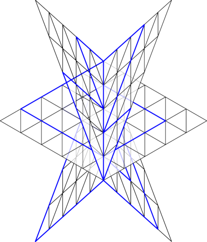
Figure 1. Examples of $K_{4}$-free bridged graphs.

2. Main ideas of the scheme

The global structure of our distance labeling scheme for $K_{4}$-free bridged graphs is similar to the one described in [17] for cube-free median graphs. Namely, the scheme is based on a recursive partitioning of the graph into a star and its fibers (which are classified as panels and cones). However, the stars and the fibers of $K_{4}$-free bridged graphs have completely different structural and metric properties from those of cube-free median graphs. Therefore, the technical tools are completely different from those used in [17].

Let $G=(V,E)$ be a $K_{4}$-free bridged graph with $n$ vertices. The encoding algorithm first searches for a median vertex $m$ of $G$, i.e., a vertex minimizing $x\mapsto\sum_{v\in V}\operatorname{d}_{G}(x,v)$. It then computes a particular $2$-neighborhood of $m$ that we call the star $\operatorname{St}(m)$ of $m$ such that every vertex of $G$ is assigned to a unique vertex of $\operatorname{St}(m)$. This allows us to define the fibers of $\operatorname{St}(m)$: for a vertex $x\in\operatorname{St}(m)$, the fiber $F(x)$ of $x$ corresponds to the set of all the vertices of $G$ associated to $x$. The set of all fibers of $\operatorname{St}(m)$ defines a partitioning of $G$. Moreover, choosing $m$ as a median vertex ensures that every fiber contains at most half of the vertices of $G$. Up to this point the scheme is the same as in [17], but here come the first differences. Namely, the fibers are not convex, nevertheless, they are connected and isometric, and thus induce bridged subgraphs of $G$. Consequently, we can apply recursively the partitioning to every fiber, without accumulating errors on distances at each step. Finally, we study the boundary and the total boundary of each fiber, i.e., respectively, the set of all vertices of a fiber having a neighbor in another fiber and the union of all boundaries of a fiber. We will see that those boundaries do not induce actual trees but something close that we call “starshaped trees”. Unfortunately, these starshaped trees are not isometric. This explains why we obtain an approximate and not an exact distance labeling scheme. Indeed, distances computed in the total boundary can be twice as much as the distances in the graph.

We distinguish two types of fibers $F(x)$ depending on the distance between $x$ and $m$: panels are fibers leaving from a neighbor $x$ of $m$; cones are fibers associated to a vertex $x$ at distance $2$ from $m$. One of our main results towards obtaining a compact labeling scheme establishes that a vertex in a panel admits two “exit” vertices on the total boundary of this panel and that a vertex in a cone admits one “entrance” vertex on each boundary of the cone (and it appears that every cone has exactly two boundaries). The median vertex $m$ or those “entrances” and “exits” of a vertex $u$ on a fiber $F(x)$ are guaranteed to lie on a path of length at most four times a shortest $(u,v)$-path for any vertex $v$ outside $F(x)$. At each recursive step, every vertex $u$ has to store information relative only to three vertices ($m$, and the two “entrances” or “exits” of $u$). Since a panel can have a linear number of boundaries, without this main property, our scheme would use labels of linear length because a vertex in a panel could have to store information relative to each boundary to allow to compute distances with constant (multiplicative) error. Since we allow a multiplicative error of $4$ at most, we will see that in almost all cases, we can return the length of a shortest $(u,v)$-path passing through the center $m$ of the star $\operatorname{St}(m)$ of the partitioning at some recursive step. Lemmas 16 and 17 indicate when this length corresponds to the exact distance between $u$ and $v$ and when it is an approximation of this distance. The case where $u$ and $v$ belong to distinct fibers that are “too close” are more technical and are the one leading to a multiplicative error of 4.

3. Preliminaries

3.1. General notions

All graphs $G=(V,E)$ in this note are finite, undirected, simple, and connected. We write $u\sim v$ if two vertices $u$ and $v$ are adjacent. For a subset $A$ of vertices of $G$, we denote by $G[A]$ the subgraph of $G$ induced by $A$. The distance $d_{G}(u,v)$ between $u$ and $v$ is the length of a shortest $(u,v)$-path in $G$. For a subset $A$ of $V$ and for two vertices $u,v\in A$, we denote by $\operatorname{d}_{A}(u,v)$ the distance $\operatorname{d}_{G[A]}(u,v)$. The interval $I(u,v)$ between $u$ and $v$ consists of all the vertices on shortest $(u,v)$–paths. In other words, $I(u,v)$ denotes all the vertices (metrically) between $u$ and $v$: $I(u,v):=\{w\in V:\operatorname{d}_{G}(u,w)+\operatorname{d}_{G}(w,v)=\operatorname{d}_{G}(u,v)\}$. Let $H=(V^{\prime},E^{\prime})$ be a subgraph of $G$. Then $H$ is called convex if $I(u,v)\subseteq H$ for any two vertices $u,v$ of $H$. The convex hull of a subgraph $H$ of $G$ is the smallest convex subgraph $\rm conv(H)$ containing $H$. A connected subgraph $H$ of $G$ is called isometric if $d_{H}(u,v)=d_{G}(u,v)$ for any vertices $u,v$ of $H$; if in addition $H$ is a cycle of $G$, we call $H$ an isometric cycle. For a vertex $x$ and a set of vertices $A\subseteq V$, let $\operatorname{d}_{G}(x,A):=\min\{\operatorname{d}_{G}(x,a):a\in A\}$ be the distance for $x$ to $A$. The metric projection of a vertex $x\in V$ on a set $A\subseteq V$ (or on $G[A]$) is the set $\text{Pr}{(x,A)}:=\{y\in A:\operatorname{d}_{G}(x,y)=\operatorname{d}_{G}(x,A)\}$. The neighborhood of $A$ in $G$ is the set $N[A]:=A\cup\{v\in V\setminus A:\exists u\in A,v\sim u\}$. The ball of radius $k$ centered at $A$ is the set $B_{k}(A):=\{v:d_{G}(v,A)\leq k\}$. When $A$ is a singleton $a$, then $N[a]$ is the closed neighborhood of $a$ and $B_{k}(a):=B_{k}(A)$. Note that $B_{1}(a)=N[a]$. The sphere of radius $k$ centered at $a$ is the set $S_{k}(A):=\{v:d_{G}(v,A)=k\}$.

3.2. Bridged graphs and metric triangles

A graph $G$ is bridged if any isometric cycle of $G$ has length 3. As shown in [21, 45], bridged graphs are characterized by one of the fundamental properties of CAT(0) spaces: the neighborhoods of all convex subgraphs of a bridged graph are convex. Consequently, balls in bridged graphs are convex. Bridged graphs constitute an important subclass of weakly modular graphs: a graph family that unifies numerous interesting classes of metric graph theory through “local-to-global” characterizations [8]. Weakly modular graphs are the graphs satisfying the following quadrangle (QC) and triangle (TC) conditions [2, 9]:

(QC) $\forall u,v,w,z\in V$ with $k:=\operatorname{d}_{G}(u,v)=\operatorname{d}_{G}(u,w)$, $\operatorname{d}_{G}(u,z)=k+1$, and $vz,wz\in E$, $\exists x\in V$ s.t. $\operatorname{d}_{G}(u,x)=k-1$ and $xv,xw\in E$.
(TC) $\forall u,v,w\in V$ with $k:=\operatorname{d}_{G}(u,v)=\operatorname{d}_{G}(u,w)$, and $vw\in E$, $\exists x\in V$ s.t. $\operatorname{d}_{G}(u,x)=k-1$ and $xv,xw\in E$.

Bridged graphs are exactly the weakly modular graphs with no induced cycle of length $4$ or $5$ [9]. Observe that, since bridged graphs do not contain induced $4$-cycles, the quadrangle condition is implied by the triangle condition.

A metric triangle $u_{1}u_{2}u_{3}$ of a graph $G=(V,E)$ is a triplet $u_{1},u_{2},u_{3}$ of vertices such that for every $(i,j,\ell)\in\{1,2,3\}^{3}$, $I(u_{i},u_{j})\cap I(u_{j},u_{\ell})=\{u_{j}\}$ [9]. A metric triangle $u_{1}u_{2}u_{3}$ is equilateral of size $k$ if $\operatorname{d}_{G}(u_{1},u_{2})=\operatorname{d}_{G}(u_{2},u_{3})=\operatorname{d}_{G}(u_{1},u_{3})=k$. If $k=0$, then the metric triangle consists of a single vertex $u_{1}=u_{2}=u_{3}$, and if $k=1$ then the vertices $u_{1}$, $u_{2}$ and $u_{3}$ are pairwise adjacent. A metric triangle $u_{1}u_{2}u_{3}$ is strongly equilateral if any $x\in I(u_{1},u_{2})$, the equality $\operatorname{d}_{G}(u_{3},x)=\operatorname{d}_{G}(u_{1},u_{2})$ holds. Weakly modular graphs can be characterized via metric triangles in the following way :

Proposition 1.

[9] A graph $G$ is weakly modular if and only if any metric triangle of $G$ is strongly equilateral.

In particular, every metric triangle of a weakly modular graph is equilateral. A metric triangle $u_{1}^{\prime}u_{2}^{\prime}u_{3}^{\prime}$ is called a quasi-median of a triplet $u_{1},u_{2},u_{3}$ if for each pair $1\leq i<j\leq 3$ there exists a shortest $(u_{i},u_{j})$-path passing via $u_{i}^{\prime}$ and $u_{j}^{\prime}$. Each triplet $u_{1},u_{2},u_{3}$ of vertices of any graph $G$ admits at least one quasi-median: it suffices to take as $u_{1}^{\prime}$ a furthest from $u_{1}$ vertex from $I(u_{1},u_{2})\cap I(u_{1},u_{3})$, as $u_{2}^{\prime}$ a furthest from $u_{2}$ vertex from $I(u_{2},u_{1}^{\prime})\cap I(u_{2},u_{3})$, and as $u_{3}^{\prime}$ a furthest from $u_{3}$ vertex from $I(u_{3},u_{1}^{\prime})\cap I(u_{3},u_{2}^{\prime})$.

3.3. Gauss-Bonet formula

We conclude this section with the classical Gauss-Bonnet formula, which will be useful in some our proofs. Let $G=(V,E)$ be a plane graph and let $\partial G$ denote the cycle delimiting its outer face. We view the inner faces of $G$ of length $k$ as regular $k$-gons of the Euclidean plane; each of their angles must be equal to $\frac{k-2}{k}\pi$. For all vertices $v$ of $G$, let $\alpha(v)$ denote the sum of the angles of the inner faces of $G$ containing $v$. In other words, if $\mathscr{C}(v)$ denotes the set of all inner faces of $G$ containing $v$, then

$$\alpha(v):=\sum_{C\in\mathscr{C}(v)}\frac{|V(C)|-2}{|V(C)|}\pi.$$

For all $v\in\partial G$, we set $\tau(v):=\pi-\alpha(v)$, and for all inner vertices $v$ of $G$ we set $\kappa(v):=2\pi-\alpha(v)$. The parameters $\kappa(v)$ and $\tau(v)$ measure the “defect” of the angles around $v$ (i.e., the gap between the actual value $\alpha(v)$ of the angles around $v$, and the value $\pi$ or $2\pi$ that should be the correct one if the polygons were “really embeddable” in the Euclidean plane). A discrete version of Gauss-Bonnet’s Theorem (see [37]) establishes the following formula (an example is given on Fig. 2):

Theorem 2 (Gauss-Bonnet).

Let $G=(V,E)$ be a planar graph. Then,

$$\sum_{v\in\partial G}\tau(v)+\sum_{v\in V\setminus\partial G}\kappa(v)=2\pi.$$

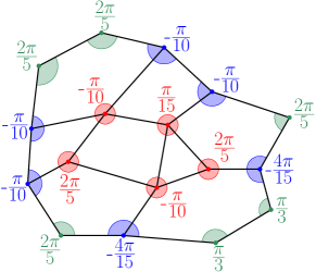
Figure 2. Gauss-Bonnet’s Theorem, and values of $\tau$ and $\kappa$ for the vertices of a planar graph $G$. The displayed values are those of $\kappa$ for the inner vertices (in red), and those of $\tau$ for the others (corners in green, and remaining vertices in blue). ${\color[rgb]{0,0,1}4\left(-\frac{\pi}{10}\right)}+{\color[rgb]{0,0,1}2\left(-\frac{4\pi}{15}\right)}+{\color[rgb]{0.1796875,0.546875,0.33984375}4\left(\frac{2\pi}{5}\right)}+{\color[rgb]{0.1796875,0.546875,0.33984375}2\left(\frac{\pi}{3}\right)}+{\color[rgb]{1,0,0}2\left(-\frac{\pi}{10}\right)}+{\color[rgb]{1,0,0}2\left(\frac{2\pi}{5}\right)}+{\color[rgb]{1,0,0}\frac{\pi}{15}}=2\pi$.

Appendix A contains a glossary with all notions and notations.

4. Metric triangles and intervals

4.1. Flat triangles and burned lozenges

From now on we suppose that $G$ is a $K_{4}$-free bridged graph. The triangular grid is a tiling of the plane with equilateral triangles of side $1$. A flat triangle is an equilateral triangle in the triangular grid; for an illustration see Fig. 3 (left). The interval $I(u,v)$ between two vertices $u,v$ of the triangular grid at distance $\ell$ induces a lozenge (see Fig. 3, right). A burned lozenge is obtained from $I(u,v)$ by iteratively removing vertices of degree $3$; equivalently, a burned lozenge is the subgraph of $I(u,v)$ in the region bounded by two shortest $(u,v)$-paths. The vertices of a burned lozenge are naturally classified into border and inner vertices. Border vertices can be articulation points of the graph defined by $I(u,v)$, see Figure 4. A non-articulation border vertex is called a convex corner if it belongs to two triangles of $I(u,v)$, and it is called a concave corner if it belongs to four triangles, see Figure 3(right). The remaining non-articulation border vertices belong to three triangles and are just called regular borders. Those vertices and the convex corners are vertices of local convexity of the burned lozenge, while concave corners are vertices of local concavity. A halved burned lozenge is the intersection of a burned lozenge with the ball $B_{k}(u)$, where $0\leq k\leq\ell$. Notice that all spheres $S_{i}(u)$ induce parallel paths of the triangular grid.

We denote the convex hull of a metric triangle $uvw$ of $G$ by $\Delta(u,v,w)$ and call it a deltoid.

We start with the following auxiliary result:

Lemma 1.

Spheres $S_{k}(u)$ of $G$ cannot contain triangles $K_{3}$.

Proof.

Suppose by way of contradiction that the vertices $x_{1},x_{2},x_{3}\in S_{k}(u)$ induce a $K_{3}$. By triangle condition, there exists a vertex $y$ adjacent to $x_{1},x_{2}$ at distance $k-1$ from $u$. For the same reason, there exists a vertex $z$ adjacent to $x_{2},x_{3}$ at distance $k-1$ from $u$. Since $G$ does not contain induced $K_{4}$, $y\neq z$ and $y\nsim x_{3},z\nsim x_{1}$. Since $y,z\in B_{k-1}(u)$ and $x_{2}\notin B_{k-1}(u)$, by the convexity of the ball $B_{k-1}(u)$, we have $y\sim z$. But then the vertices $y,z,x_{3},x_{1}$ induce a forbidden 4-cycle. ∎

The following two lemmas were known before for $K_{4}$-free planar bridged graphs (see for example, [Proposition 3] [3] for the first lemma) but their proofs remain the same. For their full proofs, see [44].

Lemma 2.

Any deltoid $\Delta(u,v,w)$ of $G$ is a flat triangle.

Proof.

We only give here some hints on how to prove the result. We can first show that $\Delta(u,v,w)$ contains a flat triangle. To do so, set $k:=\operatorname{d}_{G}(v,w)$ and consider a shortest $(v,w)$-path $P$. We rename its vertices by $v=:u_{0}^{k},u_{1}^{k},\ldots,u_{k}^{k}:=w$, where $u_{i}^{k}$ denotes the vertex at distance $i$ from $v=u_{0}^{k}$ on $P$. By successively applying the triangle condition to vertices $u_{0}^{0}:=u$, $u_{i}^{k}$ and $u_{i+1}^{k}$ for $i\in\{0,\ldots,k-1\}$, we derive vertices $u_{i}^{k-1}\sim u_{i}^{k},u_{i+1}^{k}$ at distance $k-1$ from $u_{0}^{0}$. Continuing so, we obtain that $\Delta(u,v,w)$ contains a flat triangle of the form:

• $V_{k}:=\{u_{i}^{j}:0\leq j\leq k\text{ and }0\leq i\leq j\}$;

• $E_{k}:=\{u_{i}^{j}u_{i^{\prime}}^{j^{\prime}}:u_{i}^{j},u_{i^{\prime}}^{j^{\prime}}\in V_{k},(j=j^{\prime}\text{ and }i^{\prime}=i-1)\text{ or }(j^{\prime}=j-1\text{ and }i-1\leq i^{\prime}\leq i)\}$.

It then remains to show that this flat triangle is vertex-maximal. This is done by proving that it is locally convex (and thus convex). ∎

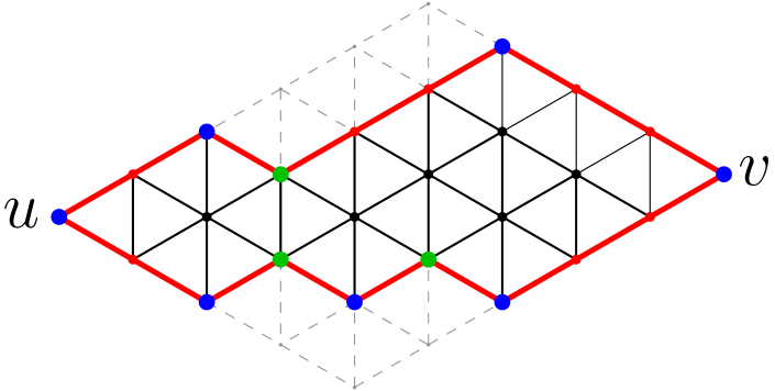
Figure 3. A flat triangle (left) and a burned lozenge (right). The concave corners are in green and convex ones are drawn in blue. The border is in red and the inner vertices in black.

Figure 4. The five red vertices indicate types of articulation points.

Lemma 3.

Any interval $I(u,v)$ of $G$ induces a burned lozenge.

Proof.

Let $u$ and $v$ be two vertices at distance $\ell$ of a $K_{4}$-free bridged graph $G$. Let $C_{i}:=\{w\in I(u,v):d_{G}(u,w)=i\}$ for $0\leq i\leq\ell$. We first show the following claim.

Claim 1.

For all $0\leq i\leq\ell$, $C_{i}$ induces a convex path of $G$.

Proof.

Observe that vertices of $C_{i}$ are at distance $\ell-i$ from $v$ and so $C_{i}=B_{i}(u)\cap B_{\ell-i}(v)$. Since $B_{i}(u)$ and $B_{\ell-i}(v)$ are both convex, $C_{i}$ is also convex, and thus $G[C_{i}]$ is a bridged subgraph. By Lemma 1, $G[C_{i}]$ cannot contains triangles, thus $G[C_{i}]$ is a tree. Suppose that this tree contains a vertex $x$ with three neighbors $x_{1},x_{2},x_{3}$. Let $y_{j}$ be the common neighbor of $x$ and $x_{j}$, $j=1,2,3$, at distance $i-1$ from $u$ (obtained by applying the triangle condition). Since $C_{i}$ is convex, the vertices $y_{1},y_{2},y_{3}$ are pairwise distinct. Since $y_{1},y_{2},y_{3}\in B_{i-1}(u)$ and $x\notin B_{i-1}(u)$, the convexity of $B_{i-1}(u)$ implies that $y_{1},y_{2},y_{3}$ are pairwise adjacent. Together with $x$ they induce a forbidden $K_{4}$. This establishes that $C_{i}$ is a convex path. ∎

Further, we will suppose that $I(u,v)$ does not contain articulation points, otherwise, we can apply the induction hypothesis to each 2-connected component of $I(u,v)$. We now show by induction on $1\leq k\leq\ell$ that the intersection $I(u,v)\cap B_{k}(u)$ is a halved burned lozenge in which all spheres $I(u,v)\cap S_{i}(u),1\leq i\leq k$ are vertical paths. For this, suppose that $u$ is identified with the origin of the triangular grid. Note that $I(u,v)\cap B_{1}(u)$ is a triangle $u,w^{\prime},w^{\prime\prime}$. We embed this triangle in the triangular grid in such a way that $w^{\prime}w^{\prime\prime}=I(u,v)\cap S_{1}(u)$ is a vertical edge to the right of $u$. Assume by induction hypothesis that the desired embedding property is satisfied for $k-1$, in particular, that $C_{k-1}=I(u,v)\cap S_{k-1}(u)$ is embedded as a vertical path. By Claim 1, $C_{k-1}$ and $C_{k}$ induce convex paths of $G$. From their definition and by Claim 1, each vertex of $C_{k-1}$ is adjacent to at least one and to at most two vertices of $C_{k}$ and, vice versa, each vertex of $C_{k}$ is adjacent to at least one and to at most two vertices of $C_{k-1}$. This implies that the lengths of paths $C_{k}$ and $C_{k-1}$ differ by at most 1. Suppose that $C_{k-1}$ induces the path $P=(u_{0},u_{1},\dots,u_{p})$ for some $p\geq 1$. For $1\leq i\leq p$, by the triangle condition, there exists a vertex $v_{i}\in C_{k}$ at distance $\ell-k$ from $v$ and adjacent to $u_{i-1},u_{i}$. By Claim 1, all $v_{i}$ are distinct. For $1\leq i\leq p-1$, $v_{i}$ and $v_{i+1}$ are adjacent since they are both adjacent to $u_{i+1}$ and $C_{k}$ is convex by Claim 1. Hence, the vertices $v_{1},\ldots,v_{p}$ define a subpath $P^{\prime}$ of $C_{k}$. If $C_{k}=P^{\prime}$, then one can extends the halved burned lozenge representing $I(u,v)\cap B_{k-1}(u)$ to a one representing $I(u,v)\cap B_{k}(u)$ by embedding the path $P^{\prime}$ vertically to the right of the path $P$. Now suppose that $P^{\prime}\neq C_{k}$. Since any vertex of $C_{k}$ is adjacent to at least one vertex of $C_{k-1}$ and each vertex of $C_{k-1}$ is adjacent to at most two vertices of $C_{k}$, we conclude that $C_{k}\setminus P^{\prime}$ may contains either one vertex $x$ or two vertices $x,y$. In the first case, $x$ is adjacent to $v_{1}$ (or to $v_{p}$) and to $u_{0}$ (or to $u_{p}$). In the second case, $x$ is adjacent to $v_{1}$ and $u_{0}$ and $y$ is adjacent to $v_{p}$ and $u_{p}$. In the first case, we add the vertical edge $xv_{1}$ or $v_{p}x$ to $P^{\prime}$. In the second edge, we add the vertical edges $xv_{1}$ and $yv_{p}$ to $P^{\prime}$. In both cases, we obtain the representation of $I(u,v)\cap B_{k}(u)$ as a halved burned lozenge. If $k=\ell$, then this halved burned lozenge will be a burned lozenge. ∎

Lemma 4.

If $uvx^{\prime}$ is the quasi-median of the triplet $uvx$, and if $w$ is a neighbor of $u$ in $I(u,v)$, then $\operatorname{d}_{G}(w,x)=\operatorname{d}_{G}(u,x)=\operatorname{d}_{G}(v,x)$.

Proof.

From the definition of the quasi-median, and since $uvx^{\prime}$ is a strongly equilateral metric triangle, we deduce that $\operatorname{d}_{G}(u,x)=\operatorname{d}_{G}(v,x)=:k$ and $\operatorname{d}_{G}(w,x)\leq k$. Suppose by way of contradiction that $\operatorname{d}_{G}(w,x)<k$, i.e., $\operatorname{d}_{G}(w,x)=k-1$. Consider the following vertices of the deltoid $\Delta(u,v,x^{\prime})$: $u_{1}$ the common neighbor of $u$ and $w$; $w_{1}$ the common neighbor of $w$ and $u_{1}$; and $u_{2}$ the common neighbor of $u_{1}$ and $w_{1}$, see Figure 5. Since $\operatorname{d}_{G}(w,x)=\operatorname{d}_{G}(u_{1},x)=k-1$, by triangle condition, there exists a vertex $t\sim u_{1},w$ having distance $k-2$ to $x$. Since $w$ is not adjacent to $u_{2}$, because of Lemma 2, $t$ is different from $u_{2}$. By convexity of the ball $B_{k-2}(x)$, we deduce that $t\sim u_{2}$. The four-cycle $\{w,t,u_{2},w_{1}\}$ can not be induced. Since $w\not\sim u_{2}$, we conclude that $w_{1}\sim t$. Consequently, the vertices $w$, $t$, $u_{2}$, $w_{1}$ induce a forbidden $K_{4}$. ∎

Figure 5. Illustration of Lemma 4.

4.2. Starshaped trees

We now introduce starshaped sets and trees, and we describe the structure of the intersection of an interval and a starshaped tree. Let $T$ be a tree rooted at a vertex $z$. A path $P$ of $T$ is called increasing if it is entirely contained on a single branch of $T$, i.e., if $\forall u,v\in P$, either $I_{T}(u,z)\subseteq I_{T}(v,z)$, or $I_{T}(v,z)\subseteq I_{T}(u,z)$. Equivalently, an increasing path is the shortest path between two vertices that are in ancestor-descendant relation. A subset $S$ of the vertices of a graph $G$ is said to be starshaped relatively to a vertex $z\in S$ if $I(z,s)\subseteq S$ for all $s\in S$. If, additionally, every $I(z,s)$ induces a single path of $G$, then $S$ is called a starshaped tree (rooted at $z\in S$), and each interval $I(z,s)$ is called a branch of $S$. Taking the union of all branches, a starshaped tree $S$ rooted at $z$ is a shortest-path spanning tree of $G[S]$ rooted at $z$. Similarly to other shortest-path trees (e.g., BFS trees), starshaped trees are not necessarily induced subgraphs of $G$, see Figure 9.

Let $I(u,z)$ be a burned lozenge which is not a single shortest path of $G$. Then $I(u,z)$ contains a non-trivial block, i.e., a $2$-connected component of $G$ containing a triangle. Let $B$ be such a non-trivial block closest to $z$. Let $z_{0}$ be the vertex of $B$ the closest to $z$ and let $u_{0}$ be the vertex of $B$ the closest to $u$. The boundary of $B$ defines two shortest $(z_{0},u_{0})$-paths $Q_{1}$ and $Q_{2}$. Let $v_{1}$ (resp. $v_{2}$) be the closest to $z$ convex corner of $I(u,z)$ belonging to $Q_{1}$ (resp. to $Q_{2}$). We call the convex corners $v_{1}$ and $v_{2}$ extremal relatively to $z$.

Lemma 5.

Let $T$ be a starshaped tree of $G$ (rooted at $z$), and let $u\in V\setminus T$. Then $T^{\prime}:=I(u,z)\cap T$ is a starshaped tree. Moreover, $T^{\prime}$ is a tripod consisting of the union of three increasing paths $P_{0}$, $P_{1}$ and $P_{2}$ such that (see Figure 6):

1. $P_{0}=I(z,z_{0})$, $P_{1}=I(z_{0},v_{1})$, and $P_{2}=I(z_{0},v_{2})$;

2. $I(z,v_{1})=P_{0}\cup P_{1}$ and $I(z,v_{2})=P_{0}\cup P_{2}$;

3. $z_{0}$, $v_{1}$, and $v_{2}$ are defined with respect to the non-trivial block $B$ closest to $z$.

Proof.

Since $T^{\prime}\subseteq T$, $T^{\prime}$ is a forest. Pick two vertices $v$ and $w$ of $T^{\prime}$. Then $v\in I(u,z)$ implies that $I(v,z)\subseteq I(u,z)$. Since $v$ belongs to $T$ and $T$ is starshaped, necessarily $I(v,z)\subseteq T$. It follows that $I(v,z)\subseteq T^{\prime}$ and $I(w,z)\subseteq T^{\prime}$. Consequently, $T^{\prime}$ is a starshaped tree.

To prove the second assertion, first notice that, since $u\notin T^{\prime}$, $I(u,z)$ is not a single shortest path. This means that the graph induced by $I(u,z)$ contains non-trivial blocks. Therefore the vertices $z_{0}$, $v_{1}$, $v_{2}$ and the paths $P_{0}$, $P_{1}$, $P_{2}$ are well defined. Moreover, $P_{0}\cup P_{1}\cup P_{2}\subseteq T^{\prime}$ as a consequence of Lemma 3 and the definition of the paths $P_{0},P_{1}$ and $P_{2}$. To prove the converse inclusion $T^{\prime}\subseteq P_{0}\cup P_{1}\cup P_{2}$, suppose by way of contradiction that there exists a vertex $v\in T^{\prime}\setminus(P_{0}\cup P_{1}\cup P_{2})$. Then $I(v,z)$ is an increasing path. From the structure of $I(u,z)$ given by Lemma 3 and from the choice of $v\in T^{\prime}\setminus(P_{0}\cup P_{1}\cup P_{2})$, we conclude that $v$ is a regular border or a convex corner of the block $B$. Suppose without loss of generality that $v$ belongs to the same border path as $v_{1}$ (see Figure 6). Since $v\neq v_{1}$, $I(v,z)\cap B$ is non-trivial, and thus $I(v,z)$ is not a single path, contrary to the assumption that $v\in T^{\prime}$. This establishes the converse inclusion, and thus $T^{\prime}=P_{0}\cup P_{1}\cup P_{2}$. ∎

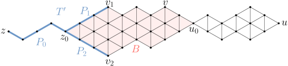
Figure 6. Illustration of Lemma 5.

5. Stars and fibers

5.1. Projections and stars

Let $z\in V$ be an arbitrary vertex of $G$. Since $G$ is bridged, $N[z]$ is convex. Note that for any $u\in V\setminus N[z]$, $z$ cannot belong to the metric projection $\text{Pr}{(u,N[z])}$. Indeed, $z$ necessarily has a neighbor $z^{\prime}$ on a shortest $(u,z)$-path. This $z^{\prime}$ is closer to $u$ than $z$, and it belongs to $N[z]$. The projections on $N[z]$ have the following property.

Lemma 6.

$\text{Pr}{(u,N[z])}$ consists of a single vertex or of two adjacent vertices. Moreover, if $d_{G}(u,z)=k+1$ and $\text{Pr}{(u,N[z])}=\{y,y^{\prime}\}$, then there exists a unique vertex $x$ adjacent to $y$ and $y^{\prime}$ and having distance $k$ to $u$.

Proof.

Notice first that $z\notin\text{Pr}{(u,N[z])}$ because any neighbor of $z$ in $I(z,u)$ is closer to $u$ than $z$. Suppose that $\text{Pr}{(u,N[z])}$ contains two distinct vertices $y$ and $y^{\prime}$. Since $y$ and $y^{\prime}$ are different from $z$, they have distance $k$ to $u$. By convexity of the ball $B_{k}(u)$, we conclude that $y$ and $y^{\prime}$ are adjacent. If $\text{Pr}{(u,N[z])}$ contains a third vertex $y^{\prime\prime}$, then $y,y^{\prime},y^{\prime\prime},z$ induce a forbidden $K_{4}$.

So, let $\text{Pr}{(u,N[z])}=\{y,y^{\prime}\}$. Then $d_{G}(u,y)=d_{G}(u,y^{\prime})=k$. Since $y\sim y^{\prime}$, by triangle condition, there exists a vertex $x\sim y,y^{\prime}$ and having distance $k-1$ to $u$. If there exists another such vertex $x^{\prime}$, since $x$ and $x^{\prime}$ belong to the ball $B_{k-1}(u)$ and are adjacent $y$ and $y^{\prime}$, there must be adjacent because $B_{k-1}(u)$ is convex. Consequently, the vertices $x,x^{\prime},y,y^{\prime}$ induce a forbidden $K_{4}$. ∎

Let $u\in V$ be a vertex with two vertices $y,y^{\prime}$ in $\text{Pr}{(u,N[z])}$. By Lemma 6, there exists a vertex $u^{\prime}\sim y,y^{\prime}$ at distance $\operatorname{d}_{G}(y,u)-1$ from $u$. Moreover, $I(u^{\prime},z)=\{u^{\prime},z,y,y^{\prime}\}$ and $y\sim y^{\prime}$. The star $\operatorname{St}(z)$ of a vertex $z\in V$ consists of the neighborhood $N[z]$ of $z$ plus all $u^{\prime}\notin N[z]$ having two neighbors $y$ and $y^{\prime}$ in $N[z]$ (which are necessarily adjacent). Consequently, $\operatorname{St}(z)$ contains the vertices of $N[z]$ and all $u^{\prime}$ that can be derived by the triangle condition applied to two adjacent vertices $y,y^{\prime}\in N[z]$ and a vertex $u\in V$. Figure 7 (1) and (2) presents two examples of stars in $K_{4}$-free bridged graphs.

(1)

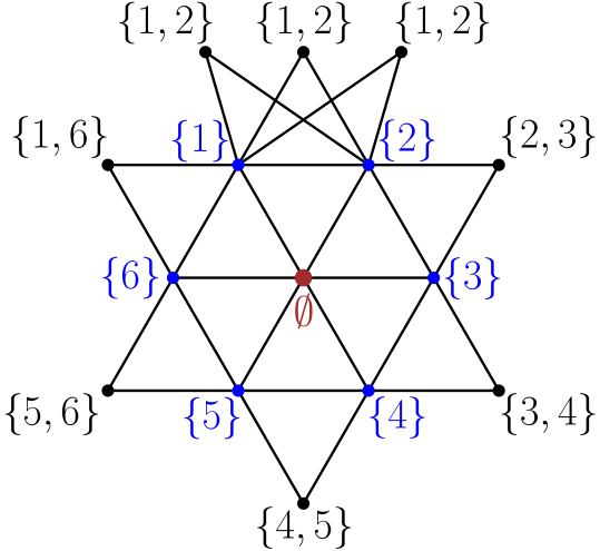
(2)

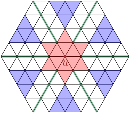
(3)

Figure 7. Examples (1) and (2) of a star and the encoding of the vertices of a star. Example (3) of cones (in blue) and panels (in green). The star of $u$ is given in red.

5.2. Cones and panels

Let $x\in\operatorname{St}(z)$. If $x\in N[z]$, we define the fiber $F(x)$ of $x$ with respect to $\operatorname{St}(z)$ as the set of all vertices of $G$ having $x$ as unique projection on $N[z]$ by Lemma 6. Otherwise (if $\operatorname{d}_{G}(x,z)=2$) $F(x)$ denotes the set of all vertices $u$ such that $\text{Pr}{(u,N[z])}$ consists of two adjacent vertices $v$ and $w$, and such that $x$ is adjacent to $v,w$ and is one step closer to $u$ than $v$ and $w$. A fiber $F(x)$ such that $x\sim z$ is called a panel. If $\operatorname{d}_{G}(x,z)=2$, then $F(x)$ is called a cone. Figure 7 (3) illustrates cones and panels. Two fibers $F(x)$ and $F(y)$ are called $k$-neighboring if $\operatorname{d}_{\operatorname{St}(z)\setminus\{z\}}(x,y)=k$. Notice that any cone is $1$-neighboring exactly two panels.

Lemma 7.

Each fiber $F(x),x\in\operatorname{St}(z)$ is starshaped with respect to $x$.

Proof.

Pick $u\in F(x)$ and $w\in I(u,x)$. Then $\text{Pr}{(w,N[z])}\subseteq\text{Pr}{(u,N[z])}$. If $F(x)$ is a panel then $x$ is the unique projection of $u$ on $N[z]$. Since $w\in I(u,x)$, $x$ is also the unique projection of $w$ on $N[z]$. Thus $w$ belongs to $F(x)$. If $F(x)$ is a cone, then the projection of $u$ on $N[z]$ consists of two vertices $x_{1}$, $x_{2}$ both adjacent to $z$ and $x$. Again, since $w\in I(u,x)$, $x_{1}$ and $x_{2}$ are projections of $w$ on $N[z]$, yielding $w\in F(x)$. ∎

Lemma 8.

Let $u\in F(x),v\in F(y)$ and $F(x)\neq F(y)$. If the fibers $F(x)$ and $F(y)$ are both cones or are both panels, then the vertices $u$ and $v$ are not adjacent.

Proof.

Suppose $u\sim v$. Notice that this implies that $\operatorname{d}_{G}(u,x)=\operatorname{d}_{G}(v,y)=:k$. Indeed, if $\operatorname{d}_{G}(u,x)>k$, then $y\in\text{Pr}{(u,\operatorname{St}(z))}$ and if $\operatorname{d}_{G}(u,x)<k$, then $x\in\text{Pr}{(v,\operatorname{St}(z))}$.

First, let $F(x)$ and $F(y)$ be two cones. If $F(y)$ and $F(y)$ are 1-neighboring $F(x)$, then $x\sim y$ and $G$ will contain a forbidden $C_{5},C_{4}$, or $K_{4}$. If $F(x)$ and $F(y)$ are 2-neighboring, then there exists a vertex $w\in\operatorname{St}(z)$ adjacent to $x$ and $y$ and at distance $k+1$ to $u$ and $v$. Then $x,y\in B_{k}(\{u,v\})$ and $w\notin B_{k}(\{u,v\})$, contrarily to convexity of $B_{k}(\{u,v\})$. Thus, the cones $F(x)$ and $F(y)$ are $r$-neighboring for some $r>2$. This implies that $\text{Pr}{(u,N[z])}\cap\text{Pr}{(v,N[z])}=\varnothing$. By the triangle condition, there exists a vertex $t\sim u,v$ at distance $k+1$ from $z$. Since $t\in I(u,z)\cap I(v,z)$, we conclude that $\text{Pr}{(t,N[z])}\subseteq\text{Pr}{(u,N[z])}\cap\text{Pr}{(v,N[z])}$. This is impossible since $\text{Pr}{(t,N[z])}\neq\varnothing$ and $\text{Pr}{(u,N[z])}\cap\text{Pr}{(v,N[z])}=\varnothing$. Now, let $F(x)$ and $F(y)$ be two panels. Then $\text{Pr}{(u,N[z])}=\{x\}$ and $\text{Pr}{(v,N[z])}=\{y\}$ and thus $\text{Pr}{(u,N[z])}\cap\text{Pr}{(v,N[z])}=\varnothing$. Since $\operatorname{d}_{G}(u,x)=\operatorname{d}_{G}(v,y)=k$ and $\operatorname{d}_{G}(u,z)=\operatorname{d}_{G}(v,z)=k+1$, $x,y\in B_{k}(\{u,v\})$ and $z\notin B_{k}(\{u,v\})$. Since $u\sim v$, $B_{k}(\{u,v\})$ is convex, $x$ and $y$ must be adjacent. Since $u$ and $v$ are adjacent and are at distance $k+1$ from $z$, by triangle condition, there exists a vertex $t\sim u,v$ with $\operatorname{d}_{G}(t,z)=k$. Since $t\in I(u,z)\cap I(v,z)$, we have $\text{Pr}{(t,N[z])}\subseteq\text{Pr}{(u,N[z])}\cap\text{Pr}{(v,N[z])}=\varnothing$, which is impossible. ∎

Lemma 9.

Let $u\in F(x),v\in F(y)$, and $u\sim v$. If $F(y)$ is a cone and $F(x)$ is a panel, then $x\sim y$ and $\operatorname{d}_{G}(u,y)=\operatorname{d}_{G}(u,x)\in\{k,k+1\}$, where $k:=\operatorname{d}_{G}(v,y)$.

Proof.

Since $u$ and $v$ are adjacent, $\operatorname{d}_{G}(u,y)\leq k+1$. By Lemma 7 $F(y)$ is starshaped with respect to $y$ and $v\in F(y),u\notin F(y)$, thus $\operatorname{d}_{G}(u,y)\geq k$. Consequently, $\operatorname{d}_{G}(u,y)\in\{k,k+1\}$. Let $y_{1}$ and $y_{2}$ denote the two neighbors of $y$ in $\operatorname{St}(z)$. Then $\operatorname{d}_{G}(v,y_{1})=\operatorname{d}_{G}(v,y_{2})=k+1$ and $\operatorname{d}_{G}(v,z)=k+2$.

First suppose that $x$ coincides with $y_{1}$ or $y_{2}$, say $x=y_{2}$. Therefore, $x\sim y$ and $\operatorname{d}_{G}(v,x)=k+1$. It remains to show that in this case $\operatorname{d}_{G}(u,y)=\operatorname{d}_{G}(u,x)$. Let $x^{\prime}$ be a neighbor of $x$ in $I(x,u)$. If $\operatorname{d}_{G}(u,x)=k$, then $y,x^{\prime}\in B_{k}(v)$ and $x\notin B_{k}(v)$. By the convexity of $B_{k}(v)$, $y$ and $x^{\prime}$ are adjacent. This implies that $\operatorname{d}_{G}(u,y)\leq k$. Since $\operatorname{d}_{G}(u,y)\geq k$, we conclude that $\operatorname{d}_{G}(u,y)=k=\operatorname{d}(u,x)$. Now suppose that $\operatorname{d}_{G}(u,x)=k+1$. If $\operatorname{d}_{G}(u,y)=k$, then this would imply that $u$ must belong to the cone $F(y)$, a contradiction. This establishes the assertion of the lemma when $x\in\{y_{1},y_{2}\}$.

We show that $x\in\{y_{1},y_{2}\}$. Assume by contradiction that $x$ is different from $y_{1}$ and $y_{2}$. This implies that $\operatorname{d}_{G}(v,x)>k+1=\operatorname{d}_{G}(v,y_{1})=\operatorname{d}_{G}(v,y_{2})$ and since $v\sim u$, we conclude that $\operatorname{d}_{G}(u,x)\geq k+1$. Analogously, since $\operatorname{d}_{G}(u,y_{1})\leq k+2$ and $\operatorname{d}_{G}(u,y_{2})\leq k+2$ and are both longer than $\operatorname{d}_{G}(u,x)$, we must have $\operatorname{d}_{G}(u,x)=k+1$ (and $\operatorname{d}_{G}(u,y_{1})=\operatorname{d}_{G}(u,y_{2})=k+2$). Thus $\operatorname{d}_{G}(u,z)=k+2=\operatorname{d}(v,z)$. Consider the ball $B_{k+1}(\{u,v\})$ of radius $k+1$ around the convex set $\{u,v\}$, which must be convex. Since $y_{2},y_{2},x\in B_{k+1}(\{u,v\})$ and $z\notin B_{k+1}(\{u,v\})$, the convexity of $B_{k+1}(\{u,v\})$ implies that $x\sim y_{1},y_{2}$. Consequently, we obtain the forbidden $K_{4}$ induced by the vertices $y_{1},y_{2},z,x$ and thus a contradiction. ∎

5.3. Partition of $G$ into fibers

We continue by showing that the fibers of any star of $G$ defines a partition of $G$ into cones and panels.

Lemma 10.

$\mathscr{F}_{z}:=\{F(x):x\in\operatorname{St}(z)\}$ defines a partition of $G$. Any fiber $F(x)$ is a bridged isometric subgraph of $G$ and $F(x)$ is starshaped with respect to $x$.

Proof.

The fact that $\mathscr{F}_{z}$ is a partition follows from its definition. Since any isometric subgraph of a bridged graph is bridged and each fiber $F(x)$ is starshaped by Lemma 7, we have to prove that $F(x)$ is isometric. Let $u$ and $v$ be two vertices of $F(x)$. We consider a quasi-median $u^{\prime}v^{\prime}x^{\prime}$ of the triplet $u,v,x$. Since $F(x)$ is starshaped, the intervals $I(u^{\prime},x^{\prime})$, $I(x,x^{\prime})$, $I(u,u^{\prime})$, $I(v,v^{\prime}),$ and $I(v^{\prime},x^{\prime})$ are all contained in $F(x)$. Consequently, to show that $u$ and $v$ are connected in $F(x)$ by a shortest path, it suffices to show that the unique shortest $(u^{\prime},v^{\prime})$-path in the deltoid $\Delta(u^{\prime},v^{\prime},x^{\prime})$ belongs to $F(x)$. To simplify the notations, we can assume two things. First, since $I(u,u^{\prime}),I(v,v^{\prime})\subseteq F(x)$, we can let $u=u^{\prime}$ and $v=v^{\prime}$. Second, we can assume that $\Delta(u,v,x^{\prime})$ is a minimal counterexample with $I(u,v)\nsubseteq F(x)$.

Let $w$ be the vertex closest to $u$ on the $(u,v)$-shortest path of $\Delta(u,v,x^{\prime})$ such that $w\notin F(x)$. Then we can suppose that $u$ is adjacent to $w$, otherwise, we can replace $u$ by the neighbor $u^{\prime}$ of $w$ in $F(x)\cap\Delta(u,v,x^{\prime})$ and obtain a smaller counterexample $\Delta(u^{\prime},v,x^{\prime})$. By Lemma 4, we conclude that $\operatorname{d}_{G}(x,u)=\operatorname{d}_{G}(x,w)=\operatorname{d}_{G}(x,v)=k$. By Lemma 2, there exist a vertex $u_{1}\sim w,u$, a vertex $w_{1}\sim u_{1},w$, and a vertex $v_{1}\sim v$ such that $w_{1}\in I(u_{1},v_{1})$. Applying Lemma 4 once again, we deduce that $\operatorname{d}_{G}(x,u_{1})=\operatorname{d}_{G}(x,w_{1})=\operatorname{d}_{G}(x,v_{1})=k-1$. By the minimality choice of the counterexample, we also deduce that the vertices $u_{1},v_{1}$ and $w_{1}$ belong to $F(x)$. Moreover, the deltoid $\Delta(u,v,x^{\prime})$ is entirely contained in $F(x)$ (see Fig. 8). Two cases have to be considered.

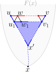
Figure 8. Illustration of the proof of Lemma 10. The minimality hypothesis implies that the blue part belongs to the fiber $F(x)$. The proof aims to show that the red shortest $(u,v)$-path also belongs to $F(x)$.

Case 1. $F(x)$ is a panel. Then, by Lemma 8, $w$ belongs to a cone $F(y)$ 1-neighboring $F(x)$. Since $\operatorname{d}_{G}(w,x)=k$, $\operatorname{d}_{G}(w,y)=k-1$. Moreover, by Lemma 9, we know that $\operatorname{d}_{G}(w_{1},y)=\operatorname{d}_{G}(w_{1},x)=k-1$. By triangle condition applied to $w$, $w_{1}$, and $y$, there exists a vertex $t\sim w,w_{1}$ at distance $k-2$ from $y$. Since $F(y)$ is starshaped and $t\in I(w,y)$, $t\in F(y)$. Also, since $F(y)$ is a cone, we obtain that $\operatorname{d}_{G}(t,x)=k-1$. By the convexity of $B_{k-1}(x)$, $t$ must coincide with $u_{1}$ or with $w_{1}$ (otherwise, the quadruplet $u_{1},w_{1},w,t$ would induce a $K_{4}$). Since $u_{1}$ and $w_{1}$ belong to $F(x)$, then $t\in F(x)$, leading to a contradiction.

Case 2. $F(x)$ is a cone. Then $w$ belongs to a panel $F(y)$ 1-neighboring $F(x)$, and this case is quite similar to the previous one. By Lemma 9, $\operatorname{d}_{G}(w,y)=\operatorname{d}_{G}(w,x)=k$. Recall that $\operatorname{d}_{G}(w_{1},x)=k-1$, $w_{1}\in F(x)$ and $F(x)$ is a cone. Consequently $\operatorname{d}_{G}(w_{1},y)=k$. We thus have $\operatorname{d}_{G}(w,y)=\operatorname{d}_{G}(w_{1},y)=k$ and, by triangle condition, there exists a vertex $t\sim w,w_{1}$ at distance $k-1$ from $y$. Still using Lemma 9, we deduce that $\operatorname{d}_{G}(t,x)=k-1$. Since $F(y)$ is starshaped, we obtain that $t\in F(y)$, and from the convexity of the ball $B_{k-1}(x)$ we conclude that $t=w_{1}$ or $t=u_{1}$. Finally, $t\in F(x)$. ∎

If we choose the star centered at a median vertex of $G$, then the number of vertices in each fiber is bounded by $|V|/2$ (the proof is similar to the proof of [17, Lemma 10]). For an edge $uv\in E(G)$, let $W(u,v):=\{w:d_{G}(u,w)<d_{G}(v,w)\}$.

Lemma 11.

If $z$ is a median vertex of $G$, then for all $x\in\operatorname{St}(z)$, $|F(x)|\leq|V|/2$.

Proof.

Suppose by way of contradiction that $|F(x)|>n/2$ for some vertex $x\in\operatorname{St}(z)$. Let $u$ be a neighbor of $z$ in $I(x,z)$. If $v\in F(x)$, then $x\in I(v,z)$ and $u\in I(x,z)$, and we conclude that $u\in I(v,z)$. Consequently, $F(x)\subseteq W(u,z)$, whence $|W(u,z)|>n/2$. Therefore $|W(z,u)|=n-|W(u,z)|<n/2$. But this contradicts the fact that $z$ is a median of $G$. Indeed, since $u\sim z$, one can easily show that $M(u)-M(z)=|W(c,z)|-|W(u,z)|<0$. ∎

6. Boundaries and total boundaries of fibers

6.1. Starshapeness of total boundaries

Let $x$ and $y$ be two vertices of $\operatorname{St}(z)$. The boundary $\partial_{F(y)}F(x)$ of $F(x)$ with respect to $F(y)$ is the set of all vertices of $F(x)$ having a neighbor in $F(y)$. The total boundary $\partial^{*}F(x)$ of $F(x)$ is the union of all its boundaries (see Fig. 9).

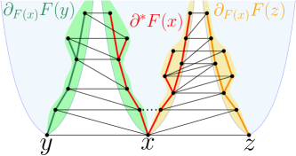
Figure 9. The boundaries $\partial_{F(x)}F(y)$ and $\partial_{F(x)}F(z)$ and of the total boundary $\partial^{*}F(x)$. The edges of this starshaped tree are indicated in red. The black dotted edge links two vertices of the starshaped tree but is not in the tree.

Lemma 12.

The total boundary $\partial^{*}F(x)$ of any fiber $F(x)$ is a starshaped tree.

Proof.

To show that $\partial^{*}F(x)$ is a starshaped tree, it suffices to show that (1) for every $v\in\partial^{*}F(x)$ the interval $I(v,x)$ is contained in $\partial^{*}F(x)$, and (2) $v$ has a unique neighbor in $I(v,x)$. By Lemma 7, $F(x)$ is starshaped, thus $I(v,x)$ is contained in $F(x)$.

First let $F(x)$ be a cone. Then $x$ has distance $2$ to $z$, and $x$ and $z$ have exactly two common neighbors $y$ and $y^{\prime}$. Let $u$ be a neighbor of $v$ in a fiber 1-neighboring $F(x)$. By Lemma 8, $u$ necessarily belongs to a panel $F(y)$ or $F(y^{\prime})$, say $u\in F(y)$. Also, we assume that $u$ is a closest to $y$ neighbor of $v$ in $F(y)$. Let $k:=\operatorname{d}_{G}(v,x)$. By the definition of a cone, we have $\operatorname{d}_{G}(v,y)=\operatorname{d}_{G}(v,y^{\prime})=k+1$ and $\operatorname{d}_{G}(v,z)=k+2$. This implies that $\operatorname{d}_{G}(u,y)\geq k$. Since $u$ belongs to the panel $F(y)$, $\operatorname{d}_{G}(u,x)\geq\operatorname{d}_{G}(u,y)$. Let $u^{\prime}$ be an arbitrary neighbor of $u$ in $I(u,y)$. If $\operatorname{d}_{G}(u,y)=k+1$, from $\operatorname{d}_{G}(u^{\prime},y)=\operatorname{d}_{G}(v,x)=k$, $\operatorname{d}_{G}(u,x)\geq\operatorname{d}_{G}(u,y)=k+1$, and from the convexity of $B_{k}(\{x,y\})$, we conclude that $u^{\prime}\sim v$. This contradicts the choice of $u$. So $\operatorname{d}_{G}(u,y)=k$. Pick any neighbor $w$ of $v$ in $I(v,x)\subset F(x)$. We assert that $w\sim u$. This would imply that $w\in\partial^{*}F(x)$ and since $G$ is $K_{4}$-free that $v$ has a unique neighbor in $I(v,x)$. Indeed, $\operatorname{d}_{G}(y,w)=\operatorname{d}_{G}(y,u)=k$ and $\operatorname{d}_{G}(y,v)=k+1$. From the convexity of the ball $B_{k}(y)$, we obtain that $w\sim u$. This establishes that $I(v,x)$ is a path included in $\partial^{*}F(x)$. Notice also that the unique neighbor $w$ of $v$ in $I(v,x)$ must be adjacent to every neighbor $u^{\prime}$ of $u$ in $I(u,y)$ because $u^{\prime},w\in B_{k-1}(\{x,y\})$. Indeed, since $u\sim u^{\prime},w$ and $\operatorname{d}_{G}(u,x)=\operatorname{d}_{G}(u,y)=k$, from the convexity of $B_{k-1}(\{x,y\})$ we conclude that $u^{\prime}\sim w$.

Now let $F(x)$ be a panel and pick any vertex $u\in\partial^{*}F(x)$. As in previous case, we have to show that $I(u,x)\subseteq\partial^{*}F(x)$ and that $u$ has a unique neighbor in $I(u,x)$. Let $v$ be a neighbor of $u$ in a fiber $F(y)$ 1-neighboring $F(x)$. By Lemma 8, $F(y)$ is a cone such that $y\sim x,x^{\prime}$, with $x^{\prime}\sim x$ and $z\sim x,x^{\prime}$. Assume that $v$ is a closest to $y$ neighbor of $u$ in $F(y)$. Let $\operatorname{d}_{G}(v,y):=k$. By Lemma 9, $\operatorname{d}_{G}(u,x)\in\{k,k+1\}$. If $\operatorname{d}_{G}(u,x)=k$, then we deduce that $u$ is adjacent to the neighbor $w$ of $v$ in $I(v,y)$, contrary to the choice of $v$. Thus $\operatorname{d}_{G}(u,x)=k+1$. In that case, if $u^{\prime}$ denotes a neighbor of $u$ in $I(u,x)$, then $\operatorname{d}_{G}(u^{\prime},x)=\operatorname{d}_{G}(v,y)=k$ and $\operatorname{d}_{G}(u,y)\geq\operatorname{d}_{G}(u,x)=k+1$. From the convexity of $B_{k}(\{y,x\})$, we conclude that $u^{\prime}\sim v$. This implies that, if $u$ has two neighbors $u^{\prime}$ and $u^{\prime\prime}$ in $I(u,x)$, then $u$, $u^{\prime}$, $u^{\prime\prime}$, and $v$ induce a forbidden $K_{4}$. Consequently, $I(u,x)$ is a path included in $\partial^{*}F(x)$. ∎

Total boundaries of fibers are starshaped trees. The following result is a corollary of Lemma 12.

Corollary 1.

Let $x$ be an arbitrary vertex of $\operatorname{St}(z)$. Then, for every pair $u,v$ of vertices of $\partial^{*}F(x)$, $\operatorname{d}_{G}(u,v)\leq\operatorname{d}_{\partial^{*}F(x)}(u,v)\leq 2\cdot\operatorname{d}_{G}(u,v)$.

Proof.

Let $(u^{\prime},v^{\prime},x^{\prime})$ be a quasi-median of $(u,v,x)$. Then $\operatorname{d}_{G}(u,v)=\operatorname{d}_{G}(u,u^{\prime})+\operatorname{d}_{G}(u^{\prime},v^{\prime})+\operatorname{d}_{G}(v^{\prime},v)$. Since ${\partial^{*}F(x)}$ is a starshaped tree by Lemma 12, $\operatorname{d}_{\partial^{*}F(x)}(u,u^{\prime})=\operatorname{d}_{G}(u,u^{\prime})$, $\operatorname{d}_{\partial^{*}F(x)}(v,v^{\prime})=\operatorname{d}_{G}(v,v^{\prime})$, $\operatorname{d}_{\partial^{*}F(x)}(u^{\prime},x^{\prime})=\operatorname{d}_{G}(u^{\prime},x^{\prime})$, and $\operatorname{d}_{\partial^{*}F(x)}(x^{\prime},v^{\prime})=\operatorname{d}_{G}(x^{\prime},v^{\prime})$. Moreover, $x^{\prime}\in I(u,x)\cap I(v,x)$ implies that $x^{\prime}$ is the nearest common ancestor of $u$ and $v$ in ${\partial^{*}F(x)}$. Since metric triangles are equilateral in bridged graphs, $\operatorname{d}_{\partial^{*}F(x)}(u^{\prime},x^{\prime})+\operatorname{d}_{\partial^{*}F(x)}(x^{\prime},v^{\prime})=2\operatorname{d}_{G}(u^{\prime},v^{\prime})$, yielding the required inequality. ∎

6.2. Projections on total boundaries

We now describe the structure of metric projections of the vertices on the total boundaries of fibers. Then in Lemma 15 we prove that vertices in panels have a constant number of “exits” on their total boundaries, even if the panel itself may have an arbitrary number of 1-neighboring cones.

Lemma 13.

Let $F(x)$ be a fiber and $u\in V\setminus F(x)$. Then the metric projection $\Pi:=\text{Pr}{(u,F(x))}=\text{Pr}{(u,\partial^{*}F(x))}$ is an induced tree of $G$.

Proof.

The metric projection of $u$ on $F(x)$ necessarily belongs to a boundary, that is a starshaped tree by Lemma 12. As a consequence, $\Pi$ is a starshaped forest, i.e., a set of starshaped trees. We assert that in fact $\Pi$ is a connected subgraph of $T:=\partial^{*}F(x)$. To prove this, we will prove the stronger property that $\Pi$ is an induced tree of $G$. Assume by way of contradiction that two vertices $v,w$ of $\Pi$ are not connected in $T$ by a path. First suppose that $w$ is an ancestor of $v$ in $T$. Then every vertex $z$ on the branch of $v$ between $v$ and $w$ belongs to a shortest $(v,w)$-path (because $T$ is starshaped) and is at distance at most $k:=\operatorname{d}_{G}(u,v)=\operatorname{d}_{G}(u,w)$ from $u$ (because the ball $B_{k}(u)$ is convex). But then we conclude that the whole shortest $(v,w)$-path belongs to $\Pi$, contrary to the choice of $v,w$. Therefore, further we can suppose that $v$ and $w$ belong to distinct branches of $T$.

Let $t$ be the nearest common ancestor of $v$ and $w$ in $T$. Let $v^{\prime}w^{\prime}t^{\prime}$ be a quasi-median of $v$, $w$, and $t$. Since $T$ is a starshaped tree, $t^{\prime}\in I(v,t)\cap I(w,t)$, and $t$ is the nearest common ancestor of $v$ and $w$, we conclude that $t=t^{\prime}$. We assert that the set of all vertices of $T$ between $v$ and $v^{\prime}$, between $v^{\prime}$ and $w^{\prime}$, and between $w^{\prime}$ and $w$ belongs to $\Pi$. Indeed, such vertices belong to a shortest $(v,w)$-path. The ball $B_{k}(u)$ is convex and $v,w\in B_{k}(u)$. Since all such vertices also belong to $T$, we conclude that they all have distance $k$ from $u$. We now show that $v^{\prime}=w^{\prime}=t$. Assume by way of contradiction that $v^{\prime}\neq w^{\prime}$ and consider an edge $ab$ on the path between $v^{\prime}$ and $w^{\prime}$ in $\Delta(v^{\prime},w^{\prime},t)$. According to Proposition 1, $\operatorname{d}_{G}(a,x)=\operatorname{d}_{G}(b,x)=:\ell$. By the triangle condition applied to $a$, $b$ and $x$, there exists a vertex $c\sim a,b$ at distance $\ell-1$ from $x$. Since $a\sim b$ and $\operatorname{d}_{G}(a,u)=\operatorname{d}_{G}(b,u)=k$, there must exist a vertex $d\sim a,b$ at distance $k-1$ from $u$ and this vertex belongs to a fiber $F(y)$ 1-neighboring $F(x)$. By Lemma 8, one of those two fibers has to be a panel and the other must be a cone.

First, let $F(x)$ be a panel and $F(y)$ be a cone. By Lemma 9, two subcases have to be considered : $\operatorname{d}_{G}(d,y)=\ell$ and $\operatorname{d}_{G}(d,y)=\ell-1$. If $\operatorname{d}_{G}(d,y)=\ell$, then $\operatorname{d}_{G}(d,y)=\operatorname{d}_{G}(y,c)=\ell$ and $\operatorname{d}_{G}(b,y)=\ell+1$. The convexity of $B_{\ell}(y)$ implies that $c\sim d$, and therefore $\{a,b,c,d\}$ induce a forbidden $K_{4}$. If $\operatorname{d}_{G}(d,y)=\ell-1$, consider the vertex $x^{\prime}\sim y,x$ in $I(z,y)$. Then $\operatorname{d}_{G}(d,x^{\prime})=\operatorname{d}_{G}(c,x^{\prime})=\ell$, but $\operatorname{d}_{G}(b,x^{\prime})=\ell+1$. From the convexity of $B_{\ell}(x^{\prime})$, we deduce that $c\sim d$. So $\{a,b,c,d\}$ induces a forbidden $K_{4}$.

Now, let $F(x)$ be a cone and $F(y)$ be a panel. By Lemma 9, we have to consider the subcases $\operatorname{d}_{G}(d,y)=\ell$ and $\operatorname{d}_{G}(d,y)=\ell+1$. If $\operatorname{d}_{G}(d,y)=\ell$, then $\operatorname{d}_{G}(d,y)=\operatorname{d}_{G}(c,y)=\ell$ and $\operatorname{d}_{G}(b,y)=\ell+1$ lead to $c\sim d$ by the convexity of $B_{\ell}(y)$. Consequently, $\{a,b,c,d\}$ induces a $K_{4}$. Finally, if $\operatorname{d}_{G}(d,y)=\ell+1$, we consider a vertex $e\sim d$ in $F(y)$ on a shortest $(d,y)$-path, and we consider the vertex $y^{\prime}\sim x,y$ in $I(x,z)$. Then $\operatorname{d}_{G}(b,y^{\prime})=\operatorname{d}_{G}(e,y^{\prime})=\ell+1$ and $\operatorname{d}_{G}(d,y^{\prime})=\ell+2$. From the convexity of $B_{\ell+1}(y^{\prime})$, it follows that $e\sim b$. With similar arguments, we show that $a\sim e$. Consequently, $\{a,b,d,e\}$ induces a forbidden $K_{4}$. Summarizing, we showed that in all cases the assumption $v^{\prime}\neq w^{\prime}$ leads to a contradiction. Therefore $v^{\prime}=w^{\prime}=t$ and $t\in\Pi$. Since $t$ is an ancestor of $v$ and $w$, by what has been shown above, $v$ and $w$ can be connected in $\Pi$ to $t$ by shortest paths. This leads to a contradiction with the assumption that $v$ and $w$ are not connected in $\Pi$. ∎

Lemma 14.

Let $F(x)$ be a fiber and $u\in V\setminus F(x)$. There exists a unique vertex $u^{\prime}\in\Pi:=\text{Pr}{(u,F(x))}$ that is closest to $x$. Furthermore, $\operatorname{d}_{G(\Pi)}(u^{\prime},v)\leq\operatorname{d}_{G}(u,u^{\prime})=\operatorname{d}_{G}(u,v)$ for all $v\in\Pi$.

Proof.

The uniqueness of $u^{\prime}$ follows from the fact that $\Pi$ is a rooted starshaped subtree of $T:=\partial^{*}F(x)$, which itself is a starshaped tree rooted at $x$. Indeed, every pair $(a,b)$ of vertices of $\Pi$ admits a nearest common ancestor in $\Pi$ that coincides with the nearest common ancestor in $T$. This ancestor has to be closer to $x$ than $a$ and $b$ (or at equal distance if $a=x$ or $b=x$).

Pick $v\in\Pi$. The equality $k:=\operatorname{d}_{G}(u,u^{\prime})=\operatorname{d}_{G}(u,v)$ holds since $\Pi$ is the metric projection of $u$ on $F(x)$. Assume by way of contradiction that $\operatorname{d}_{G}(u^{\prime},v)\geq k+1$. Then $I(v,u^{\prime})=:P$ is an increasing path of length at least $k+1$ in a starshaped tree. By triangle condition applied to $u$ and to every pair of neighboring vertices of $P$, we derive at least $k$ vertices. We then can show that each of these (at least $k$) vertices has to be distinct from every other (otherwise, $P$ would contain a shortcut). We also can prove that those vertices create a path and, by induction on the length of this new shortest path, deduce that $(u,v,t)$ forms a non-equilateral metric triangle, which is impossible. ∎

6.3. The distance lemma

Lemma 14 establishes that every branch of the tree $\Pi$ has depth smaller or equal to $\operatorname{d}_{G}(u,u^{\prime})$. The vertex $u^{\prime}$ defined in Lemma 14 will be called the entrance of vertex $u$ in the fiber $F(x)$.

Lemma 15.

Let $u$ be any vertex of $G$ and let $T$ be a starshaped tree rooted at $z\in V$. Let $u_{1}$ and $u_{2}$ be the two extremal vertices with respect to $z$ in the two increasing paths of $I(u,z)\cap T$ (there are at most two of them by Lemma 5). Then, for all $v\in T$, the following inequality holds

$$\min\{\operatorname{d}_{G}(u,u_{1})+\operatorname{d}_{T}(u_{1},v),\operatorname{d}_{G}(u,u_{2})+\operatorname{d}_{T}(u_{2},v)\}\leq 2\cdot\operatorname{d}_{G}(u,v).$$

Proof.

Assume $\min_{i\in\{1,2\}}\{\operatorname{d}_{G}(u,u_{i})+\operatorname{d}_{T}(u_{i},v)\}$ is reached for $i=1$. Let $x\in T$ be the nearest common ancestor of $u_{1}$ and $v$. By Lemma 5, we know that $v\notin I(u,z)$, unless $v=x$. We can assume that $v\neq x$, otherwise $\operatorname{d}_{G}(u,v)=\operatorname{d}_{G}(u,u_{1})+\operatorname{d}_{T}(u_{1},v)$ would be shown already. Consider a quasi-median $u^{\prime}v^{\prime}z^{\prime}$ of the triplet $u,v,z$ (see Fig. 11, left). We can make the following two remarks:

(1) Since $T$ is a starshaped tree and $I(z,v)$ is one of its branches, $v^{\prime}$ necessarily belongs to $I(z,v)$. If $v^{\prime}\in I(z,x)$, then $v^{\prime}\in I(u_{1},z)\cap I(v,z)$ implies that $v^{\prime}=x$ and that $\operatorname{d}_{G}(u,u_{1})+\operatorname{d}_{T}(u_{1},v^{\prime})+\operatorname{d}_{T}(v^{\prime},v)=\operatorname{d}_{G}(u,v)$. Indeed, if $v^{\prime}=x$, then $v^{\prime}\in I(u,z)$ (because $x\in I(u,z)$). So $\operatorname{d}_{G}(u,u_{1})+\operatorname{d}_{G}(u_{1},v^{\prime})=\operatorname{d}_{G}(u,v^{\prime})$. Since $T$ is starshaped, $\operatorname{d}_{G}(u_{1},v^{\prime})=\operatorname{d}_{T}(u_{1},v^{\prime})$ and $\operatorname{d}_{T}(v^{\prime},v)=\operatorname{d}_{G}(v^{\prime},v)$. Finally, since $v^{\prime}$ belongs to a quasi-median of $u,v,z$, $v^{\prime}$ lies on a shortest $(u,v)$-path. So $\operatorname{d}_{G}(u,u_{1})+\operatorname{d}_{T}(u_{1},v^{\prime})+\operatorname{d}_{T}(v^{\prime},v)=\operatorname{d}_{G}(u,v^{\prime})+\operatorname{d}_{G}(v^{\prime},v)=\operatorname{d}_{G}(u,v)$. Therefore, $v^{\prime}\in I(x,v)$.

(2) Since $T$ is starshaped and $z^{\prime}\in I(v,z)$, $z^{\prime}$ belongs to the branch $I(v,z)$ of $T$. Since $z^{\prime}\in I(u,z)$ $I(x,v)\cap I(u,z)=\{x\}$, we conclude that $z^{\prime}$ is between $z$ and $x$. Since $z^{\prime}\in I(u^{\prime},z)\cap I(u_{1},z)$, and $u_{1},u^{\prime}\in I(u,z)$, we assert that $\operatorname{d}_{G}(u,u^{\prime})+\operatorname{d}_{G}(u^{\prime},z^{\prime})=\operatorname{d}_{G}(u,u_{1})+\operatorname{d}_{T}(u_{1},z^{\prime})$. Indeed, $u^{\prime}\in I(u,z^{\prime})$ because it belongs to a quasi-median of $u,v,z$ ; $u_{1}\in I(u,z^{\prime})$ by definition, so the distance between $u$ and $z^{\prime}$ passing through $u_{1}$ and passing through $u^{\prime}$ are equal: $\operatorname{d}_{G}(u,u^{\prime})+\operatorname{d}_{G}(u^{\prime},z)=\operatorname{d}_{G}(u,u_{1})+\operatorname{d}_{G}(u_{1},z^{\prime})$. Finally, since $T$ is starshaped (and $z^{\prime}\in T$), $\operatorname{d}_{G}(u_{1},z^{\prime})=\operatorname{d}_{T}(u_{1},z^{\prime})$.

Since the quasi-median $u^{\prime}v^{\prime}z^{\prime}$ is an equilateral metric triangle, we have

$$2\cdot\operatorname{d}_{G}(u,v) \geq\operatorname{d}_{G}(u,u^{\prime})+\operatorname{d}_{G}(u^{\prime},z^{\prime})+\operatorname{d}_{T}(z^{\prime},v)$$

$$=\operatorname{d}_{G}(u,u_{1})+\operatorname{d}_{G}(u_{1},z^{\prime})+\operatorname{d}_{T}(z^{\prime},v)$$

$$=\operatorname{d}_{G}(u,u_{1})+\operatorname{d}_{T}(u_{1},v).$$

This concludes the proof. ∎

Stated informally, Lemma 15 asserts that if $u\in F(x)$ and $T:=\partial^{*}F(x)$, then the shortest paths from $u$ to any vertex of $T$ are “close” to a path passing via $u_{1}$ or via $u_{2}$. The vertices $u_{1}$ and $u_{2}$ are called the exits of vertex $u$. If $u$ stores the information relative to the exits $u_{1}$ and $u_{2}$, then approximate distances between $u$ and all vertices of $T$ can be easily computed.

Remark 1.

The inequality of Lemma 15 is tight as shown by vertices $u$ and $v$ from Figure 10.

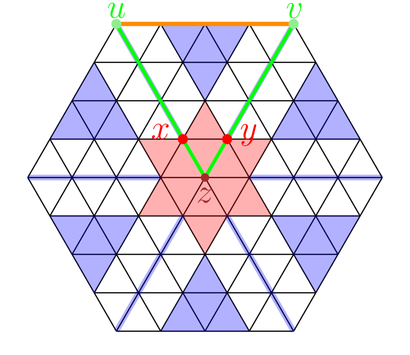
Figure 10. The vertices $u$ and $v$ coincide with their respective exits.

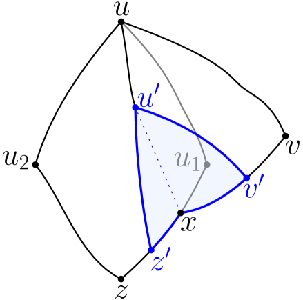
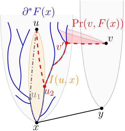
Figure 11. Notations of Lemma 15 (left) and illustration of the entrance and exits used in Lemma 18 (right).

7. Shortest paths and classification of pairs of vertices

In this section, we characterize the pairs of vertices of $G$ which are connected by a shortest path passing via the center $z$ of $\operatorname{St}(z)$ (Lemma 16). We also exhibit the cases for which passing via $z$ can lead to a multiplicative error $2$ (Lemma 17). Finally, we present the cases where our algorithm could make an error of at most $4$ (Lemma 18). In this last case, our analysis might not be tight.

Let $x$ and $y$ be two vertices of $\operatorname{St}(m)$ and let $(u,v)\in F(x)\times F(y)$. If $F(x)=F(y)$, then $u$ and $v$ are called close. When $F(x)$ and $F(y)$ are as described in Lemma 16, i.e., if $z\in I(u,v)$, then $u$ and $v$ are called separated. If $F(x)$ and $F(y)$ are 1-neighboring, one of the fibers being a panel and the other a cone, then $u$ and $v$ are called 1pc-neighboring. If $F(x)$ and $F(y)$ denote two 2-neighboring cones, then $u$ and $v$ are 2cc-neighboring. In remaining cases, $u$ and $v$ are said to be almost separated.

7.1. Separated vertices

For separated vertices $u,v$, clearly $\operatorname{d}_{G}(u,z)+\operatorname{d}_{G}(z,v)$ is just the distance $\operatorname{d}_{G}(u,v)$. Next lemma establishes which pairs of vertices are separated.

Lemma 16.

Let $u\in F(x)$ and $v\in F(y)$. Then $z\in I(u,v)$ iff $F(x)$ and $F(y)$ are distinct and either: (i) both are panels and are $k$-neighboring, for $k\geq 2$; (ii) one is a panel and the other is a $k$-neighboring cone, for $k\geq 3$; (iii) both are cones and are $k$-neighboring, for $k\geq 4$.

Proof.

Consider a quasi-median $u^{\prime}v^{\prime}z^{\prime}$ of the triplet $u,v,z$. The vertex $z$ belongs to a shortest $(u,v)$-path if and only if $u^{\prime}=v^{\prime}=z^{\prime}=z$. In that case, let $s\in I(u,z)$ and $t\in I(v,z)$ be two neighbors of $z$. Since $z$ belongs to a shortest $(u,v)$-path, $s$ and $t$ cannot be adjacent. It follows (see Fig. 12) that $F(x)$ and $F(y)$ are $k$-neighboring with: (i) $k\geq 2$ if $F(x)$ and $F(y)$ are both panels; (ii) $k\geq 3$ if one of $F(x)$ and $F(y)$ is a cone, and the other a panel; (iii) $k\geq 4$ if $F(x)$ and $F(y)$ are both cones.

For the converse implication, we consider the cases where $z$ does not belong to a shortest $(u,v)$-path. First notice that if $F(x)=F(y)$, then $z$ cannot belong to such a shortest path because, then, $\operatorname{d}_{G}(u,v)\leq\operatorname{d}_{G}(u,x)+\operatorname{d}_{G}(x,v)<\operatorname{d}_{G}(u,z)+\operatorname{d}_{G}(z,v)$. We now assume that $F(x)\neq F(y)$. Three cases have to be considered depending on the type of $F(x)$ and $F(y)$.

Case 1. $F(x)$ and $F(y)$ are both panels. If $z=z^{\prime}$, then according to Lemma 2, $x$ and $y$ must be the two neighbors of $z$, respectively lying on the shortest $(z,u^{\prime})$- and $(z,v^{\prime})$-paths, and $x\sim y$, i.e., $F(x)$ and $F(y)$ are 1-neighboring. If $z\neq z^{\prime}$, we consider a vertex $z^{\prime\prime}\in I(z,z^{\prime})$ adjacent to $z$. Then $z^{\prime\prime},x\in I(u,z)$ and, since $u$ belongs to a panel, $z^{\prime\prime}=x$. With the same arguments, we obtain that $z^{\prime\prime}=y$. Consequently, $F(x)=F(y)$, contrary to our assumption.

Case 2. $F(x)$ is a cone and $F(y)$ is a panel (the symmetric case is similar). Let $x^{\prime}$ and $x^{\prime\prime}$ denote the two neighbors of $x$ in the interval $I(x,z)$. If $z=z^{\prime}$, then by Lemma 2, $y$ and $x^{\prime}$ (or $x^{\prime\prime}$) must belong to the deltoid $\Delta(u^{\prime},v^{\prime},z^{\prime})$ and then $x^{\prime}\sim y$ (or $x^{\prime\prime}\sim y$). It follows that $F(x)$ and $F(y)$ are 2-neighboring. If $z\neq z^{\prime}$, we consider again a neighbor $z^{\prime\prime}$ of $z$ in $I(z,z^{\prime})$. Since $x^{\prime},x^{\prime\prime}\in I(u,z)$, $z^{\prime\prime}$ must coincide with $x^{\prime}$ or with $x^{\prime\prime}$, say $z^{\prime\prime}=x^{\prime}$. Also, $z^{\prime\prime}=y$. Consequently, $F(x)$ and $F(y)$ are 1-neighboring.

Case 3. $F(x)$ and $F(y)$ are both cones. Let $x^{\prime}$ and $x^{\prime\prime}$ denote the two neighbors of $x$ in $I(x,z)$, and let $y^{\prime}$ and $y^{\prime\prime}$ be those of $y$ in $I(z,y)$. Again, if $z=z^{\prime}$, then $x^{\prime}$ (or $x^{\prime\prime}$) and $y^{\prime}$ (or $y^{\prime\prime}$) belong to the deltoid $\Delta(u^{\prime},v^{\prime},z^{\prime})$, leading to $x^{\prime}\sim y^{\prime}$ and to the fact that $F(x)$ and $F(y)$ are 3-neighboring. If $z\neq z^{\prime}$, we consider $z^{\prime\prime}\in I(z,z^{\prime})$, $z^{\prime\prime}\sim z$. By arguments similar to those used in previous cases, we obtain that $z^{\prime\prime}=x^{\prime}=y^{\prime}$ (up to a renaming of the vertices $x^{\prime\prime}$ and $y^{\prime\prime}$). It follows that $F(x)$ and $F(y)$ are 2-neighboring. ∎

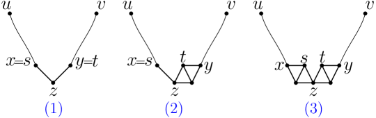
Figure 12. Illustration of the proof of Lemma 16.

7.2. Almost separated vertices

The following lemma show that in case of almost separated vertices, $\operatorname{d}_{G}(u,z)+\operatorname{d}_{G}(z,v)$ is still a good approximation of the distance $\operatorname{d}_{G}(u,v)$:

Lemma 17.

Let $u\in F(x)$ and $v\in F(y)$ be almost separated. Then, $\operatorname{d}_{G}(u,v)\leq\operatorname{d}_{G}(u,z)+\operatorname{d}_{G}(z,v)\leq 2\cdot\operatorname{d}(u,v).$

Proof.

Let $u^{\prime}v^{\prime}z^{\prime}$ be a quasi-median of the triplet $u,v,z$. We have to show that $z=z^{\prime}$. According to Lemma 16, four cases must be considered: $F(x)$ and $F(y)$ are two 1-neighboring or 2-neighboring fibers of distinct types and $F(x)$ and $F(y)$ are two 3-neighboring cones.

First, let $F(x)$ and $F(y)$ be 1-neighboring, one of them being a panel and the other a cone. If $x$ and $y$ belong to a shortest $(u,v)$-path, then $z=z^{\prime}$. Let us assume that this is not the case. Then there exists a cone $F(w)\sim F(x),F(y)$ such that $I(u,v)\cap F(w)\neq\varnothing$. We claim that, if $z^{\prime}\notin F(w)$, then $z=z^{\prime}$. Indeed, this directly follows from the fact that $z^{\prime}\in I(u,z)\cap I(v,z)$, $x\notin I(v,z)$ and $y\notin I(u,z)$. We now show that $z^{\prime}\notin F(w)$. Indeed, notice that $x\notin I(v,z)$, $y\notin I(u,z)$, and $x,y\in I(w,z)$ imply that $w\notin I(u,z)\cup I(v,z)$. By the definition of $u^{\prime}v^{\prime}z^{\prime}$, we obtain that $z^{\prime}\in I(u,z)$. If $z^{\prime}\in F(w)$, this would contradicts that $w\in I(z^{\prime},z)\subseteq I(u,z)$. Hence $z=z^{\prime}$ in this case as well.

Let now $F(x)$ and $F(y)$ be 2-neighboring, one of them being a panel and the other a cone. Suppose that $F(y)$ is the panel and denote by $x_{1}$ and $x_{2}$ the two neighbors of $x$ in $I(x,z)$. Then in the same way as before, we show that $z=z^{\prime}$. Indeed, $z^{\prime}\in I(u,z)$ requires that $z^{\prime}\in F(x)\cup F(x_{1})\cup F(x_{2})\cup\{z\}$, and $z^{\prime}\in I(v,z)$ requires that $z^{\prime}\in F(y)\cup\{z\}$. Consequently, $z=z^{\prime}$.

Finally, let $F(x)$ and $F(y)$ be two 3-neighboring cones. Let $x_{1},x_{2}\in I(x,z)$ and $y_{1},y_{2}\in I(y,z)$ be distinct from $x$, $y$, $z$, and each others. Again, $z^{\prime}\in I(u,z)$ leads to $z^{\prime}\in F(x)\cup F(x_{1})\cup F(x_{2})\cup\{z\}$, and $z^{\prime}\in I(v,z)$ leads to $z^{\prime}\in F(y)\cup F(y_{1})\cup F(y_{2})\cup\{z\}$. These sets intersect only in the vertex $z$, so $z^{\prime}=z$. ∎

7.3. 1pc-Neighboring vertices

Let $F(x)$ be a panel and let $F(y)$ be a cone 1-neighboring $F(x)$. We set $T:=\partial^{*}F(x)$. Let $u\in F(x)$ and $v\in F(y)$. Recall that by Lemma 13, $\Pi:=\text{Pr}{(v,T)}$ induces a tree. The vertex $v^{\prime}$ of $\Pi$ closest to $x$ is called the entrance of $v$ on the total boundary $T$. Similarly, two vertices $u_{1}$ and $u_{2}$ such as described in Lemma 15 are called the exits of $u$ on the total boundary $T$. See Fig. 11 (right) for an illustration of the notations of this paragraph.

Lemma 18.

Let $u\in F(x)$ and $v\in F(y)$ be two 1pc-neighboring vertices, where $F(x)$ is a panel and $F(y)$ a cone. Let $T$, $u_{1}$, $u_{2}$ and $v^{\prime}$ be as described above. Then,

$$\operatorname{d}_{G}(u,v) \leq\min\{\operatorname{d}_{G}(u,u_{1})+\operatorname{d}_{T}(u_{1},v^{\prime}),\operatorname{d}_{G}(u,u_{2})+\operatorname{d}_{T}(u_{2},v^{\prime})\}+\operatorname{d}_{G}(v^{\prime},v)$$

$$\leq 4\cdot\operatorname{d}_{G}(u,v).$$

Proof.

Assume $\min\{\operatorname{d}_{G}(u,u_{1})+\operatorname{d}_{T}(u_{1},v^{\prime}),\operatorname{d}_{G}(u,u_{2})$ $+$ $\operatorname{d}_{T}(u_{2},v^{\prime})\}$ is reached for $u_{1}$. Let $u^{\prime}\in I(u,v)\cap T$ be closest possible from $\Pi$. Then the exact distance between $u$ and $v$ is $\operatorname{d}_{G}(u,u^{\prime})+\operatorname{d}_{G}(u^{\prime},v)$ and we have to compare it with $\operatorname{d}_{G}(u,u_{1})+\operatorname{d}_{T}(u_{1},v^{\prime})+\operatorname{d}_{G}(v^{\prime},v)$. By triangle inequality, we obtain:

$$\operatorname{d}_{G}(u,u_{1})+\operatorname{d}_{T}(u_{1},v^{\prime})\leq\operatorname{d}_{G}(u,u_{1})+\operatorname{d}_{T}(u_{1},u^{\prime})+\operatorname{d}_{T}(u^{\prime},v^{\prime}).$$

Since $v^{\prime}\in\Pi$, we obtain $\operatorname{d}_{G}(v^{\prime},v)\leq\operatorname{d}_{G}(u^{\prime},v)$. By the choice of $u_{1}$ and by Lemma 15, we also know that $\operatorname{d}_{G}(u,u_{1})+\operatorname{d}_{T}(u_{1},u^{\prime})\leq 2\cdot\operatorname{d}_{G}(u,u^{\prime})$. It remains to compare $\operatorname{d}_{T}(u^{\prime},v^{\prime})$ with $\operatorname{d}_{G}(u^{\prime},v)$.

Suppose first that $u^{\prime}$ and $v^{\prime}$ belong to a same branch of $T$ and consider a quasi-median $u_{0}^{\prime}v_{0}^{\prime}v_{0}$ of $u^{\prime},v^{\prime},v$. Then $I(u^{\prime},v^{\prime})\subseteq T$ (because $T$ is starshaped) leads to $u_{0}^{\prime},v_{0}^{\prime}\in T$. The vertex $u^{\prime}$ being the closest possible to $\Pi$, we have $u^{\prime}=u_{0}^{\prime}$. Since $v_{0}^{\prime}\in I(v,v^{\prime})$, $v_{0}^{\prime}\in\Pi$. Also, since $v^{\prime}$ is the closest possible to $u^{\prime}$ vertex, we have $v^{\prime}=v_{0}^{\prime}$. Finally, since each quasi-median is an equilateral metric triangle, we conclude that $\operatorname{d}_{G}(u,u^{\prime})=\operatorname{d}_{G}(u,v^{\prime})$. Consequently, $u^{\prime}\in\Pi$. All this allows us to obtain the inequalities $\operatorname{d}_{T}(u^{\prime},v^{\prime})\leq\operatorname{d}_{G}(u^{\prime},v)$ (Lemma 14), and

$$\begin{array}[]{rccccclcl}\operatorname{d}_{G}(u,v)&\leq&\operatorname{d}_{G}(u,u_{1})&+&\lx@intercol\hfil\operatorname{d}_{T}(u_{1},v^{\prime})\hfil\lx@intercol&+&\operatorname{d}_{G}(v^{\prime},v)\\ &\leq&\operatorname{d}_{G}(u,u_{1})&+&\operatorname{d}_{T}(u_{1},u^{\prime})&+&\operatorname{d}_{T}(u^{\prime},v^{\prime})&+&\operatorname{d}_{G}(v^{\prime},v)\\ &\leq&\lx@intercol\hfil 2\cdot\operatorname{d}_{G}(u,u^{\prime})\hfil\lx@intercol&+&\operatorname{d}_{G}(u^{\prime},v)&+&\operatorname{d}_{G}(u^{\prime},v)\\ &=&\lx@intercol 2\cdot\operatorname{d}_{G}(u,v).\hfil\lx@intercol\end{array}$$

Suppose now that $u^{\prime}$ and $v^{\prime}$ belong to distinct branches of $T$, and denote by $t$ their nearest common ancestor in this starshaped tree. Let $u^{\prime\prime}$ be the closest vertex to $t$ in the metric projection of $v$ on the branch of $u^{\prime}$. Consider a quasi-median $u_{0}^{\prime}v_{0}^{\prime}t_{0}$ of $u^{\prime},v^{\prime},t$. Since $T$ is starshaped, $t_{0}\in I(u^{\prime},t)\cap I(v^{\prime},t)$, and $t$ nearest common ancestor of $u^{\prime}$ and $v^{\prime}$, we conclude that $t=t_{0}$. Moreover, $u_{0}^{\prime}$ and $v_{0}^{\prime}$ belong to the branches of $u^{\prime}$ and of $v^{\prime}$, respectively. We distinguish five cases, illustrated in Fig. 13. Blue lines correspond to the exact distance $\operatorname{d}_{G}(u^{\prime},v)$, and red ones correspond to the approximate distance that we are comparing to it.

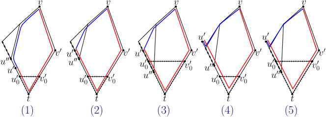
Figure 13. Illustration of the proof of Lemma 18.

In fact, we can notice that the error will be maximal if $u^{\prime}$ is the extremity opposite to $u^{\prime\prime}$ in the projection of $v$ on the branch of $u^{\prime}$. Indeed, in every considered case the error occurs on the fragment of the path between $u^{\prime}$ and $u^{\prime\prime}$ that does not belong to the shortest $(u,v)$-path. The length of this fragment is maximal in that case. We now assert that the two following inequalities hold:

Claim 2.

$\operatorname{d}_{G}(t,v^{\prime})\leq\operatorname{d}_{G}(v,u^{\prime\prime})$, and $\operatorname{d}_{G}(t,u^{\prime\prime})\leq\operatorname{d}_{G}(v,v^{\prime})$.

Proof.

Begin by noticing that $u^{\prime\prime}$ and $v^{\prime}$ belong to $I(v,t)$. Notice also that $I(t,u^{\prime\prime})\cap I(t,v^{\prime})=\{t\}$, but the intervals $I(v,u^{\prime\prime})$ and $I(v,v^{\prime})$ may intersect on some part of $I(v,t)$, not only in $\{v\}$. Let $s$ be a furthest from $v$ vertex in this intersection ($v$ and $s$ might coincide, as is the case in the illustration of the five cases above, to make it simpler). We will prove that $\operatorname{d}_{G}(s,u^{\prime\prime})=\operatorname{d}_{G}(v^{\prime},t)$, and that $\operatorname{d}_{G}(s,v^{\prime})=\operatorname{d}_{G}(u^{\prime\prime},t)$.

By Lemma 3, the interval $I(s,t)$ induces a burned lozenge, thus a plane graph. We call bigon a subgraph $D$ of this burned lozenge $I(s,t)$ bounded by two shortest $s,t$-paths, the first one passing via $u^{\prime\prime}$ and the second one passing via $v^{\prime}$ (for illustration, see Fig. 14). Note that each bigon is a burned lozenge. The area of $D$ is the number inner faces (all triangles) of $I(s,t)$ belonging to $D$.

Assume now that $D$ is a bigon with minimal area. The boundary $\partial D$ of $D$ consists of a shortest $(s,u^{\prime\prime})$-path $P_{1}$, shortest $(s,v^{\prime})$-path $P_{2}$, shortest $(t,u^{\prime\prime})$-path $Q_{1}$, and shortest $(t,v^{\prime})$-path $Q_{2}$. Notice that each corner of $D$ is either a vertex of $\partial D$ with two neighbors (corner of type 1) or a vertex of $\partial D$ with three neighbors (corner of type 2). The two neighbors of a corner of type 1 are adjacent and the three neighbors of a corner of type 2 induce a 3-path. The vertices $s$ and $t$ are corners of type 1 because they have exactly two neighbors in $I(s,t)$ by Lemma 3. We now assert that, among the remaining vertices of $\partial D$ of $D$, only $u^{\prime\prime}$ and $v^{\prime}$ can be corners. Indeed, the paths $Q_{1}$ and $Q_{2}$ between $t$ and $u^{\prime\prime},v^{\prime}$ are convex (because they belong to the branches of a starshaped tree). Consequently, $Q_{1}$ and $Q_{2}$ cannot contain corners different from $t,u^{\prime\prime}$, or $v^{\prime}$. Concerning the paths $P_{1}$ and $P_{2}$ between $s$ and $u^{\prime\prime},v^{\prime}$, suppose by way of contradiction that one of them, say $P_{1}$, contains a corner (distinct from $u^{\prime\prime}$ and $s$). If this corner is of type 1, we directly obtain a contradiction with the fact that it belongs to a shortest $(s,t)$-path. If this corner is of type 2, denote it by $a$, denote by $a^{\prime}$ its unique neighbor in the interior of $D$, and by $b$ and $c$ its neighbors in $\partial D$. Since $a^{\prime}$ is adjacent to $b$ and $c$, $a^{\prime}$ belong to a shortest $(s,t)$-path, obtained by replacing $a$ by $a^{\prime}$. Consequently, we created a bigon $D^{\prime}$ with two triangles less than $D$, contradicting the minimality of $D$.

Thus, $D$ has at most four corners, $s,t,u^{\prime\prime},$ and $v^{\prime}$. We apply to $D$ the Gauss-Bonnet formula. Since $D$ is a burned lozenge, for every $w\in D\setminus\partial D$, $\kappa(w)=0$, and for every $w\in\partial D\setminus\{s,t,v^{\prime},u^{\prime\prime}\}$, $\tau(w)=0$. Since $\tau(s)=\tau(t)=\frac{2\pi}{3}$ by the Gauss-Bonnet formula (Theorem 2), $\tau(u^{\prime\prime})+\tau(v^{\prime})=\frac{2\pi}{3}$. It follows that either $v^{\prime}$ and $u^{\prime\prime}$ are both corners of type 2, or one of them is a corner of type 1 and the other is not a corner. We can easily observe that the second case is impossible because, if one vertex is a corner of type 1, it cannot belong to a shortest $(s,t)$-path. Thus both $u^{\prime\prime}$ and $v^{\prime}$ are corners of type 2. Consequently, $D$ is a full lozenge and we conclude that $\operatorname{d}_{G}(s,u^{\prime\prime})=\operatorname{d}_{G}(v^{\prime},t)$ and $\operatorname{d}_{G}(s,v^{\prime})=\operatorname{d}_{G}(u^{\prime\prime},t)$. This finishes the proof of the claim. ∎

Returning to the proof of the lemma, from the equalities $\operatorname{d}_{G}(v,t)=\operatorname{d}_{G}(v,u^{\prime\prime})+\operatorname{d}_{G}(u^{\prime\prime},t)=\operatorname{d}_{G}(v,v^{\prime})+\operatorname{d}_{G}(v^{\prime},t)=\operatorname{d}_{G}(v,u^{\prime})+\operatorname{d}_{G}(u^{\prime\prime},t)$, we deduce that $\operatorname{d}_{G}(v,v^{\prime})+\operatorname{d}_{T}(v^{\prime},u^{\prime})<4\operatorname{d}_{G}(v,u^{\prime})$. Consequently,

$$\begin{array}[]{rcccccl}\operatorname{d}_{G}(u,v)&\leq&\operatorname{d}_{G}(u,u_{1})+\operatorname{d}_{T}(u_{1},u^{\prime})&+&\operatorname{d}_{T}(u^{\prime},v^{\prime})&+&\operatorname{d}_{G}(v^{\prime},v)\\ &\leq&2\cdot\operatorname{d}_{G}(u,u^{\prime})&+&3\cdot\operatorname{d}_{G}(u^{\prime},v)&+&\operatorname{d}_{G}(u^{\prime},v)\\ &\leq&\lx@intercol 4\cdot\operatorname{d}_{G}(u,v).\hfil\lx@intercol\end{array}$$

∎

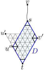
Figure 14. Illustration of the proof of Claim 2.

7.4. 2cc-Neighboring vertices

Finally, we consider the case of 2cc-neighboring vertices.

Lemma 19.

Let $u$ and $v$ be two 2cc-neighboring vertices respectively belonging to the cones $F(x)$ and $F(y)$. Let $F(w)$ denote the panel 1-neighboring $F(x)$ and $F(y)$, and set $T:=\partial^{*}F(w)$. Let $u^{\prime}$ and $v^{\prime}$ be the respective entrances of $u$ and $v$ on $T$. Then

$$\operatorname{d}_{G}(u,v)\leq\operatorname{d}_{G}(u,u^{\prime})+\operatorname{d}_{T}(u^{\prime},v^{\prime})+\operatorname{d}_{G}(v^{\prime},v)\leq 4\cdot\operatorname{d}_{G}(u,v).$$

Proof.

First we prove that there exists a shortest $(u,v)$-path traversing the panel $F(w)$. Let $w^{\prime}$ be the second common neighbor of $x$ and $z$ and $w^{\prime\prime}$ be the second common neighbor of $y$ and $z$. Let $u^{*}v^{*}w^{*}$ be a quasi-median of the triplet $u,v,w$ and let $P(u,v)$ be a shortest $(u,v)$-path passing via $u^{*}$ and $v^{*}$. Finally, let $w_{0}$ be a neighbor of $w$ in $I(w,w^{*})$. Since $w\in I(u,z)\cap I(v,z)$ and $u^{*}$ belongs to a shortest $(u,w)$-path, we conclude that $w\in I(u^{*},z)$. Moreover, $w\in I(t,z)$ for any $t\in I(u,u^{*})$. Analogously, $w\in I(t,z)$ for any $t\in I(v,v^{*})$. This implies that each of the vertices of $I(u,u^{*})\cup I(v^{*},v)$ belongs either to the panel $F(w)$ or to a cone defined by $w$ and a common neighbor of $w$ and $z$.

While moving along $P(u,v)$ from $u$ to $v$, at some point we have to leave the cone $F(x)$. Since two cones cannot be adjacent (Lemma 8), necessarily we have to move to a panel. If the first change of a fiber happens on the portion of $P(u,v)$ between $u$ and $u^{*}$, then by previous discussion, we conclude that we have to enter the panel $F(w)$ and we are done. So, suppose that $u^{*}\in F(x)$. Analogously, we can suppose that $v^{*}\in F(y)$. Thus, further we suppose that $u=u^{*}$ and $v=v^{*}$ (see Figure 15 for the notations of this proof).

Since $G$ does not contain induced $C_{4},C_{5}$, and $K_{4}$, one can easily see that $w_{0}\neq x,y$. Since $w_{0},x\in I(w,u)$ and $w_{0},y\in I(w,v)$, we conclude that $w_{0}\sim x,y$. By triangle condition applied to the edge $xw_{0}$ and $u$, we conclude that there exists $x_{1}\sim x,w_{0}$ one step closer to $u$ than $x$ and $w_{0}$. Analogously, there exists a vertex $y_{1}\sim w_{0},y$ one step closer to $v$. Let $w_{1}$ be a neighbor of $w_{0}$ in $I(w_{0},w^{*})$. If $w_{1}$ coincides with $x_{1}$ or $y_{1}$ we will obtain a forbidden $C_{4},C_{5}$, and $K_{4}$. Otherwise, since $x_{1},w_{1}\in I(w_{0},u)$ and $y_{1},w_{1}\in I(w_{0},v)$ we conclude that $w_{1}\sim x_{1},y_{1}$. Continuing this way, i.e., applying the triangle condition and the forbidden graph argument, we will construct the vertices $x_{i}\in I(x_{i-1},u)\cap I(w_{i-1},u),$ $y_{i}\in I(y_{i-1},v)\cap I(w_{i-1},v),$ and $w_{i}\in I(w_{i-1},w^{*})$, such that $x_{i}\sim x_{i-1},w_{i-1}$, $y_{i}\sim y_{i-1},w_{i-1}$, and $w_{i}\sim x_{i},y_{i},$ and $w_{i-1}$. After $p=\operatorname{d}_{G}(w_{0},w^{*})$ steps, we will have $w_{p}=w^{*}$. Let $a$ and $b$ be the unique neighbors of $w^{*}$ in $I(w^{*},u)$ and $I(w^{*},v)$, respectively (uniqueness follows from Lemma 2). Since $x_{p},w_{p}=w^{*}$ have the same distance to $u$, by triangle condition, $x_{p}\sim a$. Analogously, we conclude that $y_{p}\sim b$. By Lemma 2, $a\sim b$. The vertices $x_{p},a,b,y_{p},w_{p-1},w_{p}$ define a 5-wheel, which cannot be induced. But any additional edge leads to a forbidden $K_{4}$ or $C_{4}$. This contradiction shows that one of the portions of $P(u,v)$ between $u$ and $u^{*}$ or between $v^{*}$ and $v$ contains a vertex $v^{\prime\prime}$ of the panel $F(w)$ adjacent to a vertex of $F(x)$ or of $F(y)$. Clearly, this vertex $v^{\prime\prime}$ must belong to the total boundary $\partial^{*}F(w)$.

Then, $\operatorname{d}_{G}(u,v)=\operatorname{d}_{G}(u,v^{\prime\prime})+\operatorname{d}_{G}(v^{\prime\prime},v)$. According to Lemma 18, the two following inequalities hold:

$$\begin{array}[]{rcccl}\operatorname{d}_{G}(u,u^{\prime})&+&\operatorname{d}_{T}(u^{\prime},v^{\prime\prime})&\leq&4\cdot\operatorname{d}_{G}(u,v^{\prime\prime})\\ \operatorname{d}_{T}(v^{\prime\prime},v^{\prime})&+&\operatorname{d}_{T}(v^{\prime},v)&\leq&4\cdot\operatorname{d}_{G}(v^{\prime\prime},v)\end{array}$$

It follows that

$$\begin{array}[]{rcccc}\operatorname{d}_{G}(u,u^{\prime})+\operatorname{d}_{T}(u^{\prime},v^{\prime})+\operatorname{d}_{G}(v^{\prime},v)&\leq&\operatorname{d}_{G}(u,u^{\prime})+\operatorname{d}_{T}(u^{\prime},v^{\prime\prime})&+&\operatorname{d}_{T}(v^{\prime\prime},v^{\prime})+\operatorname{d}_{G}(v^{\prime},v)\\ &\leq&4\cdot\operatorname{d}_{G}(u,v^{\prime\prime})&+&4\cdot\operatorname{d}_{G}(v^{\prime\prime},v)\\ &=&\lx@intercol\hfil 4\cdot\operatorname{d}_{G}(u,v).\hfil\lx@intercol\end{array}$$

∎

Figure 15. Illustration of the proof of Lemma 19.

Remark 2.

Lemma 19 covers a case which was not correctly considered in the short version of this paper.

8. Distance labeling scheme

We now describe the $4$-approximate distance labeling scheme for $K_{4}$-free bridged graphs. In this section, $G=(V,E)$ is a $K_{4}$-free bridged graph with $n$ vertices.

8.1. Encoding

We begin with a brief description of the encoding of the star $\operatorname{St}(m)$ of a median vertex $m$ of $G$ (in Section 8.2, we explain how to use it to decode the distances). Then we describe the labels $\text{L}(u)$ given to vertices $u\in V$ by the encoding algorithm.

Encoding of the star. Let $m$ be a median vertex of $G$ and let $\operatorname{St}(m)$ be the star of $m$. The star-label of a vertex $u\in\operatorname{St}(m)$ is denoted by $\text{L}_{\operatorname{St}(m)}(u)$. We set $\text{L}_{\operatorname{St}(m)}(m):=0$ (where $0$ will be considered as the empty set $\varnothing$). Each neighbor of $m$ takes a distinct label in the range $\{1,\ldots,\deg(m)\}$ (interpreted as singletons). The label $\text{L}_{\operatorname{St}(m)}(u)$ of a vertex $u$ at distance $2$ from $m$ corresponds to the concatenation of the labels $\text{L}_{\operatorname{St}(m)}(u^{\prime})$ and $\text{L}_{\operatorname{St}(m)}(u^{\prime\prime})$ of the two neighbors $u^{\prime}$ and $u^{\prime\prime}$ of $u$ in $I(u,m)$, i.e., $\text{L}_{\operatorname{St}(m)}(u)$ is a set of size 2.

Remark 3.

The labels of the vertices of $\operatorname{St}(m)$ not adjacent to $m$ are not necessarily unique identifiers of these vertices. Moreover, the labeling of $\operatorname{St}(m)$ does not allow to determine adjacency of all pairs of vertices of $\operatorname{St}(m)$. Indeed, adjacency queries between vertices encoded by a singleton cannot be answered; a singleton label only tells that the corresponding vertex is adjacent to $m$, see Fig. 7, right.

Encoding of the $K_{4}$-free bridged graphs. Let $u$ denote any vertex of $G$. Let $L_{0}(u)$ be the unique identifier of $u$. We describe here the part $\text{L}_{i}(u)$ of the label of $u$ built at step $i\geq 1$ of the recursion by the encoding procedure (see Enc_Dist). $\text{L}_{i}(u)$ consists of three parts: “St”, “1st”, and “2nd”. The first part $\text{L}_{i}^{\text{St}}$ contains information relative to the star $\operatorname{St}(m)$ around the median $m$ chosen in the corresponding step: the unique identifier $\text{id}(m)=:\text{L}_{i}^{\text{St}[\text{Med}]}(u)$ of $m$ in $G$; the distance $\operatorname{d}_{G}(u,m)=:\text{L}_{i}^{\text{St}[\text{Dist}]}(u)$ between $u$ and $m$; and a star labeling $\text{L}_{\operatorname{St}(m)}(x)=:\text{L}_{i}^{\text{St}[\text{Root}]}(u)$ of $u$ in $\operatorname{St}(m)$ (where $x\in\operatorname{St}(m)$ is such that $u\in F(x)$). This last identifier is used to determine to which type of fibers the vertex $u$ belongs, as well as the status (close, separated, 1pc-neighboring, or other) of the pair $(u,v)$ for any other vertex $v\in V$. Recall that any cone has exactly two 1-neighboring panels.

The two subsequent parts, $\text{L}_{i}^{\text{1st}}$ and $\text{L}_{i}^{\text{2nd}}$, depend whether $F(x)$ is a cone or a panel. If $F(x)$ is a panel, then $\text{L}_{i}^{\text{1st}}$ and $\text{L}_{i}^{\text{2nd}}$ contain information relative to the two exits $u_{1}$ and $u_{2}$ of $u$ on the total boundary $\partial^{*}F(x)$ of $F(x)$. The part $\text{L}_{i}^{\text{1st}}$ contains (1) an exact distance labeling $\text{L}_{\partial^{*}F(x)}(u_{1})=:\text{L}_{i}^{\text{1st}[\text{Rep}]}(u)$ of $u_{1}$ in the total boundary of $F(x)$ and (2) the distance $\operatorname{d}_{G}(u,u_{1})=:\text{L}_{i}^{\text{1st}[\text{Dist}]}(u)$ between $u$ and $u_{1}$ in $G$. The part $\text{L}_{i}^{\text{2nd}}$ is the same as $\text{L}_{i}^{\text{1st}}$ with $u_{2}$ replacing $u_{1}$.

If $F(x)$ is a cone, then $\text{L}_{i}^{\text{1st}}$ and $\text{L}_{i}^{\text{2nd}}$ contain information relative to the entrances $u_{1}^{+}$ and $u_{2}^{+}$ of $u$ on (i) the total boundaries $\partial^{*}F(w_{1})$ and $\partial^{*}F(w_{2})$ of the two 1-neighboring fibers $F(w_{1})$ and $F(w_{2})$ of $F(x)$. The part $\text{L}_{i}^{\text{1st}}$ contains (1) an exact distance labeling $\text{L}_{\partial^{*}F(w_{1})}(u_{1}^{+})=:\text{L}_{i}^{\text{1st}[\text{Rep}]}(u)$ of $u_{1}^{+}$ in the starshaped tree $\partial^{*}F(w_{1})$ (the DLS described in [22], for example) and (2) the distance $\operatorname{d}_{G}(u,u_{1}^{+})=:\text{L}_{i}^{\text{1st}[\text{Dist}]}(u)$ between $u$ and $u_{1}^{+}$ in $G$. Finally, the part $\text{L}_{i}^{\text{2nd}}$ is the same as $\text{L}_{i}^{\text{1st}}$ with $u_{2}^{+}$ replacing $u_{1}^{+}$ and $\partial^{*}F(w_{2})$ instead of $\partial^{*}F(w_{1})$.

Input: A $K_{4}$-free bridged graph $G=(V,E)$, and a list $\text{L}(V):=\{\text{L}(u):=\text{L}_{0}(u)=(\text{id}(u)):u\in V\}$ of unique identifiers of its vertices.

if $V=\{v\}$ then  stop ;

Find a median vertex $m$ of $G$ ;

$\text{L}_{\operatorname{St}(m)}(\operatorname{St}(m))$ $\leftarrow$ Enc_Star ($\operatorname{St}(m)$) ;

foreach panel $F(x)\in{\mathcal{F}}_{m}$ do

       $\text{L}_{\partial^{*}F(x)}(\partial^{*}F(x))$ $\leftarrow$ Enc_Tree ($\partial^{*}F(x)$);

      

      foreach $u\in F(x)$ do

             Find the exits $u_{1}$ and $u_{2}$ of $u$ on $\partial^{*}F(x)$ ;

            

            $L^{\text{St}}\leftarrow(\text{id}(m),~{}\operatorname{d}_{G}(u,m),~{}\text{L}_{\operatorname{St}(m)}(x))$ ;

              // $L^{\text{St}}\leftarrow(L^{\text{St}[\text{Med}]},L^{\text{St}[\text{Dist}]},L^{\text{St}[\text{Root}]})$

             $L^{\text{1st}}\leftarrow(\text{L}_{\partial^{*}F(x)}(u_{1}),~{}\operatorname{d}_{G}(u,u_{1}))$ ;

              // $L^{\text{1st}}\leftarrow(L^{\text{1st}[\text{Rep}]},L^{\text{1st}[\text{Dist}]})$

             $L^{\text{2nd}}\leftarrow(\text{L}_{\partial^{*}F(x)}(u_{2}),~{}\operatorname{d}_{G}(u,u_{2}))$ ;

              // $L^{\text{2nd}}\leftarrow(L^{\text{2nd}[\text{Rep}]},L^{\text{2nd}[\text{Dist}]})$

             $\text{L}(u)\leftarrow\text{L}(u)\circ(L^{\text{St}},~{}L^{\text{1st}},~{}L^{\text{2nd}})$ ;

            

      Enc_Dist ($G[F(x)]$, $\text{L}(F(x))$) ;

      

foreach cone $F(x)\in{\mathcal{F}}_{m}$ do

       foreach $u\in F(x)$ do

             Find $w_{1},w_{2}\in\operatorname{St}(m)$ s.t. $F(w_{1})$ and $F(w_{2})$ are the two panels 1-neighboring $F(x)$ ;

             Let $u^{+}_{1}$ and $u^{+}_{2}$ be the two entrances of $u$ on $F(w_{1})$ and $F(w_{2})$ ;

            

            $L^{\text{St}}\leftarrow(\text{id}(m),~{}\operatorname{d}_{G}(u,m),~{}\text{L}_{\operatorname{St}(m)}(x))$ ;

              // $L^{\text{St}}\leftarrow(L^{\text{St}[\text{Med}]},L^{\text{St}[\text{Dist}]},L^{\text{St}[\text{Root}]})$

             $L^{\text{1st}}\leftarrow(\text{L}_{\partial^{*}F(w_{1})}(u^{+}_{1}),~{}\operatorname{d}_{G}(u,u^{+}_{1}))$ ;

              // $L^{\text{1st}}\leftarrow(L^{\text{1st}[\text{Rep}]},L^{\text{1st}[\text{Dist}]})$

             $L^{\text{2nd}}\leftarrow(\text{L}_{\partial^{*}F(w_{2})}(u^{+}_{2}),~{}\operatorname{d}_{G}(u,u^{+}_{2}))$ ;

              // $L^{\text{2nd}}\leftarrow(L^{\text{2nd}[\text{Rep}]},L^{\text{2nd}[\text{Dist}]})$

            

            $\text{L}(u)\leftarrow\text{L}(u)\circ(L^{\text{St}},~{}L^{\text{1st}},~{}L^{\text{2nd}})$ ;

            

      Enc_Dist ($G[F(x)]$, $\text{L}(F(x))$) ;

      

Algorithm 1 Enc_Dist ($G$, $\text{L}(V)$)

8.2. Distance queries

Given the labels $\text{L}(u)$ and $\text{L}(v)$ of two vertices $u$ and $v$, the distance decoder (see Distance below) starts by determining the state of the pair $(u,v)$. To do so, it looks up for the first median $m$ that separates $u$ and $v$, i.e., such that $u$ and $v$ belong to distinct fibers with respect to $\operatorname{St}(m)$. More precisely, it looks for the part $i$ of the labels corresponding to the step in which $m$ became a median. As noticed in [17, Section 6.4.6], it is possible to find this median vertex $m$ in constant time by adding particular $O(\log^{2}n)$ bits information to the head of each label (consisting of a lowest common ancestor scheme defined on the tree of median vertices). Once the right parts of label are found, the decoding function determines that two vertices are 1pc-neighboring if and only if the identifier (i.e., the star-label in $\operatorname{St}(m)$ of the fiber of one of the two vertices $u,v$ is strictly included in the identifier of the other). In that case, the decoding function calls a procedure based on Lemma 18 (see Dist_1pc-neighboring below). More precisely, the procedure returns

$$\min\{\operatorname{d}_{G}(u,u_{1})+\operatorname{d}_{T}(u_{1},v^{\prime}),\operatorname{d}_{G}(u,u_{2})+\operatorname{d}_{T}(u_{2},v^{\prime})\}+\operatorname{d}_{G}(v^{\prime},v),$$

where we assume that $u$ belongs to a panel (and $v$ belongs to a cone), where $u_{1}$, $u_{2}$ are contained in the label parts $\text{L}_{i}^{\text{2nd}}(u)$, $\text{L}_{i}^{\text{1st}}(u)$ and $v^{\prime}$ is contained in the label part $\text{L}_{i}^{\text{2nd}}(v)$ or $\text{L}_{i}^{\text{1st}}(v)$. The distances $\operatorname{d}_{T}(u_{1},v^{\prime})$ and $\operatorname{d}_{T}(u_{2},v^{\prime})$ are obtained by decoding the tree distance labels of $u_{1}$, $u_{2}$, and $v^{\prime}$ in $T$ (also available in these label parts). We also point out that we assume that $\text{L}_{i}^{\text{1st}}(v)$ always contains the information to get to the panel whose identifier corresponds to the minimum of the two values identifying the cone of $v$. The vertices $u$ and $v$ are classified as 2cc-neighboring if and only if the identifier of their respective fibers intersect in a singleton. In that case, Distance calls the procedure Dist_2cc-neighboring, based on Lemma 19. In all the remaining cases (i.e., when $u$ and $v$ are separated or almost separated), the decoding algorithm will return $\operatorname{d}_{G}(u,m)+\operatorname{d}_{G}(v,m)$. By Lemmas 16 and 17, this sum is sandwiched between $\operatorname{d}_{G}(u,v)$ and $2\cdot\operatorname{d}_{G}(u,v)$. We now give the two main procedures used by the decoding algorithm Distance: Dist_1pc-neighboring and Dist_2cc-neighboring. Note that Dist_1pc-neighboring assumes that its first argument $u$ belongs to a panel and the second $v$ belongs to a cone.

function Dist_1pc-neighboring($\text{L}_{i}(u)$, $\text{L}_{i}(v)$):

      $\text{dir}\leftarrow\text{2nd}$ ;

      // If $\text{L}_{i}^{\text{St}[\text{Root}]}(u)=\max\{j:j\in\text{L}_{i}^{\text{St}[\text{Root}]}(v)\}$

      if $\text{L}_{i}^{\text{St}[\text{Root}]}(u)=\min\{j:j\in\text{L}_{i}^{\text{St}[\text{Root}]}(v)\}$ then  $\text{dir}\leftarrow\text{1st}$ ;

      $v^{\prime}\leftarrow\text{L}_{i}^{\text{dir}[\text{Rep}]}(v)$ ;

      $u_{1},~{}u_{2}\leftarrow\text{L}_{i}^{\text{1st}[\text{Rep}]}(u),~{}\text{L}_{i}^{\text{2nd}[\text{Rep}]}(u)$ ;

      $d_{1},~{}d_{2}\leftarrow\texttt{Dist\_\allowbreak Tree}(v^{\prime},u_{1}),~{}\texttt{Dist\_\allowbreak Tree}(v^{\prime},u_{2})$ ;

      return $\text{L}_{i}^{\text{dir}[\text{Dist}]}(v)+\min\left\{d_{1}+\text{L}_{i}^{\text{1st}[\text{Dist}]}(u),~{}d_{2}+\text{L}_{i}^{\text{2nd}[\text{Dist}]}(u)\right\}$ ;

     

Recall that in the following procedure, $u$ and $v$ both belong to cones at step $i$.

function Dist_2cc-neighboring($\text{L}_{i}(u)$, $\text{L}_{i}(v)$):

      $\{x\}\leftarrow\text{L}_{i}^{\text{St}[\text{Root}]}(u)\cap\text{L}_{i}^{\text{St}[\text{Root}]}(v)$ ;

      $\text{dirU},~{}\text{dirV}\leftarrow\text{2nd},~{}\text{2nd}$ ;

      if $x=\min\{j:j\in\text{L}_{i}^{\text{St}[\text{Root}](u)}\}$  then  $\text{dirU}\leftarrow\text{1st}$ ;

      if $x=\min\{j:j\in\text{L}_{i}^{\text{St}[\text{Root}](v)}\}$  then  $\text{dirV}\leftarrow\text{1st}$ ;

      $u^{\prime},~{}v^{\prime}\leftarrow\text{L}_{i}^{\text{dirU}[\text{Rep}]}(u),~{}\text{L}_{i}^{\text{dirV}[\text{Rep}]}(v)$ ;

      $d_{u},~{}d_{v}\leftarrow\text{L}_{i}^{\text{dirU}[\text{Dist}]}(u),~{}\text{L}_{i}^{\text{dirV}[\text{Dist}]}(v)$ ;

      $d\leftarrow\texttt{Dist\_\allowbreak Tree}(u^{\prime},v^{\prime})$ ;

      return $d_{u}+d+d_{v}$ ;

     

The following algorithm Distance finds the first step where the given vertices $u$ and $v$ have belonged to distinct fibers for the first time. If they are 1pc-neighboring or 2cc-neighboring at this step, then Distance respectively calls procedure Dist_1pc-neighboring or Dist_2cc-neighboring. Otherwise, it returns the sum of their distances to the median of the step. The occurring cases are illustrated by Figure 16.

Input: The labels $\text{L}(u)$ and $\text{L}(v)$ of two vertices $u$ and $v$ of $G$

Output: A value between $\operatorname{d}_{G}(u,v)$ and $4\cdot\operatorname{d}_{G}(u,v)$

if $\text{L}_{0}(u)=\text{L}_{0}(v)$ /* $u=v$ */ then  return $0$ ;

Let $i$ be the greatest integer such that $\text{L}_{i}^{\text{St}[\text{Med}]}(u)=\text{L}_{i}^{\text{St}[\text{Med}]}(v)$ ;

// If $u$ is in a panel 1-neighboring the cone of $v$

if $\text{L}_{i}^{\text{St}[\text{Root}]}(u)\subsetneq\text{L}_{i}^{\text{St}[\text{Root}]}(v)$ then

       return $\textnormal{{Dist\_\allowbreak 1pc-neighboring}}(\text{L}_{i}(u),\text{L}_{i}(v))$ ;

      

// If $v$ is in a panel 1-neighboring the cone of $u$

if $\text{L}_{i}^{\text{St}[\text{Root}]}(v)\subsetneq\text{L}_{i}^{\text{St}[\text{Root}]}(u)$ then

       return $\textnormal{{Dist\_\allowbreak 1pc-neighboring}}(\text{L}_{i}(v),\text{L}_{i}(u))$ ;

      

// If $u$ is in a cone 2-neighboring the cone of $v$

if $|\text{L}_{i}^{\text{St}[\text{Root}]}(u)\cap\text{L}_{i}^{\text{St}[\text{Root}]}(v)|=1$ $\text{L}_{i}^{\text{St}[\text{Root}]}(u)\neq\text{L}_{i}^{\text{St}[\text{Root}]}(v)$  then

       return $\textnormal{{Dist\_\allowbreak 2cc-neighboring}}(\text{L}_{i}(u),\text{L}_{i}(v))$ ;

      

// In every other case

return $\text{L}_{i}^{\text{St}[\text{Dist}]}(u)+\text{L}_{i}^{\text{St}[\text{Dist}]}(v)$ ;

Algorithm 2 Distance ($\text{L}(u)$, $\text{L}(v)$)

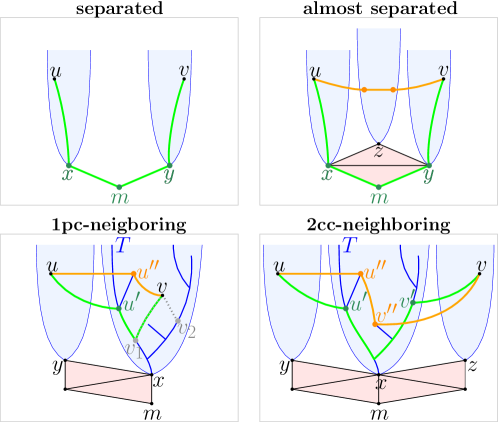
Figure 16. Decoding of the distances between separated, almost separated, 1pc-neighboring, and 2cc-neighboring vertices. An exact shortest path is given in orange, and the path considered by our decoding algorithm appears in green.

8.3. Correctness and complexity

Since by Lemma 11 the number of vertices in every part is each time divided by 2, the recursion depth is $O(\log n)$. At each recursive step, the vertices add to their label a constant number of information among which the longest consists in a distance labeling scheme for trees using $O(\log^{2}n)$ bits. It follows that our scheme uses $O(\log^{3}n)$ bits for each vertex. We show, by induction on $n$, that the time complexity is $T(n):=a(n^{2}\log n+n)$ for some constant $a$. This is trivially true for $n=1$. For a graph $G=(V,E)$ on $n$ vertices, we can compute a median vertex $m$ of $G$, and its partition into fibers $F(x_{1}),\ldots,F(x_{k})$ (with $n_{1},\ldots,n_{k}$ vertices respectively) in time $O(n^{2})$ by using the distance matrix of $G$. A vertex $u$ belongs to the total boundary of its fiber $F(x_{i})$ if one of its neighbors belongs to another fiber. This can be determined in time $O(n)$. Therefore, the total boundary of all the fibers can be computed in time $O(n^{2})$. Let $u$ be a vertex of a panel $F(x_{j})$, the interval $I(x_{j},u)$ can be computed in time $O(n)$, and thus the two exits of $u$ (i.e., the two extremal vertices of $I(x_{j},u)\cap\partial^{*}F(x_{j})$) can also be computed in time $O(n)$. Let $v$ be a vertex of a cone $F(x_{\ell})$. The projections $\text{Pr}{(v,F)}$ and $\text{Pr}{(v,F^{\prime})}$ of $v$ on the two panels $1$-neighboring $F(x_{\ell})$ can be computed in time $O(n)$, hence the two entrances of $v$ (i.e., the roots of $\text{Pr}{(v,F)}\cap\partial^{*}F$ and $\text{Pr}{(v,F^{\prime})}\cap\partial^{*}F^{\prime}$) can also be computed in time $O(n)$. Consequently, the first step of the induction requires time $an^{2}$. By induction, computing the label of all $u$ in $F(x_{i})$ takes time $T(n_{i})$. Therefore, $T(n)=an^{2}+\sum_{i=1}^{k}T(n_{i})$. By Lemma 11, $n_{i}\leq n/2$ for all $i\in\{1,\ldots,k\}$. Consequently,

$$\begin{array}[]{rcl}T(n)&=&an^{2}+\sum_{i=1}^{k}(an_{i}^{2}\log n_{i}+n_{i})\\ &\leq&an^{2}+an^{2}\log(\frac{n}{2})+an\\ &\leq&a(n^{2}\log n+n).\end{array}$$

We conclude that the total complexity of Algorithm 1 is $O(n^{2}\log n)$.

That the decoding algorithm returns distances with a multiplicative error at most $4$ directly follows from Lemmas 16 and 17 for separated and almost separated vertices, and from Lemmas 18 and 19 for the 1pc-neighboring and 2cc-neighboring vertices. Those results are based on Lemmas 14 and 15 that respectively indicate the entrances and exits to store in total boundaries of panels. This concludes the proof of Theorem 1.

9. Conclusion

We would like to finish this paper with some open questions. First of all, the problem of finding a polylogarithmic (approximate) distance labeling scheme for general bridged graphs remains open. We formulate it in the following way:

Question 1.

Do there exist constants $c$ and $b$ such that any bridged graph $G$ admits a $c$-approximate distance labeling scheme with labels of size $O(\log^{b}n)$ ?

One of the first obstacles in adapting our labeling scheme to general bridged graphs is that it is not clear how to define the star and the fibers. In all bridged graphs, since the neighborhood $N[z]$ of a vertex $z$ is convex, the metric projection of any vertex $u$ on $N[z]$ induces a clique. Therefore, we could define the fiber $F(C)$ for a clique $C$ of $N[z]$ as the set of all $u$ having $C$ as metric projection on $N[z]$. This induces a partitioning of $V(G)\setminus N[z]$, however the interaction between different fibers of $N[z]$ seems intricate.

The same question can be asked for bridged graphs of constant clique-size and for hyperbolic bridged graphs (via a result of [8], those are the bridged graphs in which all deltoids have constant size). A positive result would be interesting since Gavoille and Ly [24] established that general graphs of bounded hyperbolicity do not admit poly-logarithmic distance labeling schemes unless we allow a multiplicative error of order $\Omega(\log\log n)$, at least.

Question 2.

Do there exist linear functions $f$ and $g$ such that every $\delta$-hyperbolic bridged graph $G$ admits a $f(\delta)$-approximate distance labeling scheme with labels of size $O(\log^{g(\delta)}n)$ ?

In the full version of [17], we managed to encode the cube-free median graphs in $O(n\log n)$ time instead of $O(n^{2}\log n)$. This improvement uses a recent result of [7] allowing to compute a median vertex of a median graph in linear time. We also compute in cube-free median graphs the partition into fibers, the gates (equivalent of the entrances) and the imprints (equivalent to the exits) in fibers in linear time, with a BFS-like algorithm. Altogether, this improvement of the preprocessing time for cube-free median graphs was technically non-trivial. In the case of $K_{4}$-free bridged graph, a similar result can be expected. The first step will be to design a linear-time algorithm for computing medians in $K_{4}$-free bridged graphs. For planar $K_{4}$-free bridged graphs, such an algorithm was described in [16].

Acknowledgment

We would like to acknowledge the referees for their very careful reading of the manuscript, numerous insightful comments, and useful suggestions. This work was supported by ANR project DISTANCIA (ANR-17-CE40-0015).

Appendices

Appendix A Glossary

In the following glossary, $G$ denotes a graph of vertex set $V$ and edge set $E$ ; unless it is explicitly defined otherwise, $T$ denotes a starshaped tree rooted at $z$; $H=(V(H),E(H))$ denotes a subgraph of $G$.

Notions and notations	Definitions
Ball $B_{k}(S)$	$\{x\in V:\exists s\in S,\operatorname{d}_{G}(x,s)\leq k\}$.
Boundary $\partial_{y}F(x)$	$\{u\in F(x):\exists v\in F(y),uv\in E\}$.
Closed neighborhood $N[u]$ of $u$	$\{v\in V:uv\in E\}\cup\{u\}$.
Cone $F(x)$ w.r.t. to $\operatorname{St}(z)$	Fiber $F(x)$ w.r.t. $\operatorname{St}(z)$ with $\operatorname{d}_{G}(x,z)=2$.
Convex subgraph $H$	$\forall u,v\in V(H)$, $I(u,v)\subseteq V(H)$.
Distance $\operatorname{d}_{G}(u,v)$	Number of edges on a shortest $(u,v)$-path of $G$.
Entrance of $u$ on $T:=\partial^{*}F(x)$	Closest vertex to $x$ in $\text{Pr}{(u,T)}$.
Exit of $u$ on $T:=\partial^{*}F(x)$	Extremal vertex w.r.t. $z$ in an increasing path of $I(u,z)\cap T$.
Extremal vertex of $I(u,z)\cap T$.	First convex corner in an increasing path starting at $z$.
Fiber $F(x)$ w.r.t. $H$	$\{u\in V:x\text{ is the gate of $u$ in }H\}$.
Increasing path $P$ of $T$	Path entirely contained in a single branch of $T$.
Interval $I(u,v)$	$\{w\in V:\operatorname{d}_{G}(u,v)=\operatorname{d}_{G}(u,w)+\operatorname{d}_{G}(w,v)\}$.
Isometric subgraph $H$	$\forall u,v\in V(H),\operatorname{d}_{H}(u,v)=\operatorname{d}_{G}(u,v)$.
Locally convex subgraph $H$	$\forall u,v\in V(H)$, with $\operatorname{d}_{G}(u,v)\leq 2$, $I(u,v)\subseteq V(H)$.
Median vertex $m$	Vertex minimizing $u\mapsto\sum_{v\in V}\operatorname{d}_{G}(u,v)$.
Metric projection $\text{Pr}{(x,H)}$	$\{u\in V(H):\forall v\in V(H),\operatorname{d}_{G}(v,x)\geq\operatorname{d}_{G}(u,x)\}$.
Metric triangle $u_{1}u_{2}u_{3}$ of $G$	$u_{1},u_{2},u_{3}\in V$ s.t. $\forall i,j,k\in\{1,2,3\}$, $I(u_{i},u_{j})\cap I(u_{j},u_{k})=\{u_{j}\}$.
Panel $F(x)$ w.r.t. to $\operatorname{St}(z)$	Fiber $F(x)$ w.r.t. $\operatorname{St}(z)$ with $\operatorname{d}_{G}(x,z)=1$.
Star $\operatorname{St}(z)$	Union of $N[z]$ and of all the triangles derived from $N[z]$ using (TC).
Starshaped $H$ w.r.t. $z$	$\forall u\in V(H),I(u,z)\subseteq V(H)$.
Starshaped tree $T\subseteq G$ w.r.t. $z$	$\forall u\in V(T)$, $I(u,z)$ is a path of $T$.
Total boundary $\partial^{*}F(x)$	$\bigcup_{y\sim x}\partial_{y}F(x)$.
Triangle condition (TC)	$\forall u,v,w\in V$ with $k:=\operatorname{d}_{G}(u,v)=\operatorname{d}_{G}(u,w)$, and $vw\in E$, $\exists x\in V$ s.t. $\operatorname{d}_{G}(u,x)=k-1$ and $xv,xw\in E$.

References

- [1] R.P Anstee and M Farber. On bridged graphs and cop-win graphs. Journal of Combinatorial Theory, Series B, 44(1):22–28, 1988. URL: https://www.sciencedirect.com/science/article/pii/0095895688900937, doi:https://doi.org/10.1016/0095-8956(88)90093-7.
- [2] H.-J. Bandelt and V. Chepoi. A Helly theorem in weakly modular space. Discrete Math., 160(1-3):25–39, 1996.
- [3] H.-J. Bandelt and V. Chepoi. The algebra of metric betweenness ii: axiomatics of weakly median graphs. Europ. J. Combin., 29:676–700, 2008.
- [4] H.-J. Bandelt and V. Chepoi. Metric graph theory and geometry: a survey. Contemporary Mathematics, 453:49–86, 2008.
- [5] Hans-Jürgen Bandelt and Victor Chepoi. Decomposition andl-embedding of weakly median graphs. Eur. J. Comb., 21(6):701–714, 2000. URL: https://doi.org/10.1006/eujc.1999.0377, doi:10.1006/eujc.1999.0377.
- [6] F. Bazzaro and C. Gavoille. Localized and compact data-structure for comparability graphs. Discr. Math., 309:3465–3484, 2009.
- [7] L. Bénéteau, J. Chalopin, V. Chepoi, and Y. Vaxès. Medians in median graphs and their cube complexes in linear time. J. Comput. Syst. Sci., 126:80–105, 2022.
- [8] J. Chalopin, V. Chepoi, H. Hirai, and D. Osajda. Weakly modular graphs and nonpositive curvature. Memoirs of AMS, 268(1309):159 pp., 2020.
- [9] V. Chepoi. Classification of graphs by means of metric triangles. Metody Diskret. Analiz., pages 75–93, 96, 1989.
- [10] V. Chepoi. Graphs of some CAT(0) complexes. Adv. Appl. Math., 24:125–179, 2000.
- [11] V. Chepoi, F. F. Dragan, and Y. Vaxès. Distance and routing labeling schemes for non-positively curved plane graphs. J. Algorithms, 61:60–88, 2006.
- [12] Victor Chepoi. Bridged graphs are cop-win graphs: an algorithmic proof. J. Combin. Theory Ser. B, 69(1):97–100, 1997.
- [13] Victor Chepoi, Feodor F. Dragan, and Yann Vaxès. Center and diameter problems in plane triangulations and quadrangulations. In David Eppstein, editor, Proceedings of the Thirteenth Annual ACM-SIAM Symposium on Discrete Algorithms, January 6-8, 2002, San Francisco, CA, USA, pages 346–355. ACM/SIAM, 2002. URL: http://dl.acm.org/citation.cfm?id=545381.545427.
- [14] Victor Chepoi, Feodor F. Dragan, and Yann Vaxès. Distance-based location update and routing in irregular cellular networks. In Lawrence Chung and Yeong-Tae Song, editors, Proceedings of the 6th ACIS International Conference on Software Engineering, Artificial Intelligence, Networking and Parallel/Distributed Computing (SNPD 2005), May 23-25, 2005, Towson, Maryland, USA, pages 380–387. IEEE Computer Society, 2005. URL: https://doi.org/10.1109/SNPD-SAWN.2005.32, doi:10.1109/SNPD-SAWN.2005.32.
- [15] Victor Chepoi, Feodor F. Dragan, and Yann Vaxès. Addressing, distances and routing in triangular systems with applications in cellular networks. Wirel. Networks, 12(6):671–679, 2006. URL: https://doi.org/10.1007/s11276-006-6527-0, doi:10.1007/s11276-006-6527-0.
- [16] Victor Chepoi, Clémentine Fanciullini, and Yann Vaxès. Median problem in some plane triangulations and quadrangulations. Comput. Geom., 27(3):193–210, 2004. URL: https://doi.org/10.1016/j.comgeo.2003.11.002, doi:10.1016/j.comgeo.2003.11.002.
- [17] Victor Chepoi, Arnaud Labourel, and Sébastien Ratel. Distance and routing labeling schemes for cube-free median graphs. Algorithmica, 83(1):252–296, 2021. URL: https://doi.org/10.1007/s00453-020-00756-w, doi:10.1007/s00453-020-00756-w.
- [18] Victor Chepoi and Damian Osajda. Dismantlability of weakly systolic complexes and applications. Trans. Amer. Math. Soc., 367(2):1247–1272, 2015. URL: http://dx.doi.org/10.1090/S0002-9947-2014-06137-0, doi:10.1090/S0002-9947-2014-06137-0.
- [19] B. Courcelle and R. Vanicat. Query efficient implementation of graphs of bounded clique-width. Discrete Appl. Math., 131:129–150, 2003.
- [20] Tomasz Elsner. Isometries of systolic spaces. Fund. Math., 204(1):39–55, 2009. URL: http://dx.doi.org/10.4064/fm204-1-3, doi:10.4064/fm204-1-3.
- [21] M. Farber and R. E. Jamison. On local convexity in graphs. Discr. Math., 66(3):231–247, 1987.
- [22] O. Freedman, P. Gawrychowski, P. K. Nicholson, and Oren Weimann. Optimal distance labeling schemes for trees. In PODC, pages 185–194. ACM, 2017.
- [23] C. Gavoille, M. Katz, N. A. Katz, C. Paul, and D. Peleg. Approximate distance labeling schemes. In ESA, pages 476–487. Springer, 2001.
- [24] C. Gavoille and O. Ly. Distance labeling in hyperbolic graphs. In International Symposium on Algorithms and Computation, pages 1071–1079. Springer, 2005.
- [25] C. Gavoille and C. Paul. Distance labeling scheme and split decomposition. Discr. Math., 273:115–130, 2003.
- [26] C. Gavoille and C. Paul. Optimal distance labeling for interval graphs and related graph families. SIAM J. Discr. Math., 22:1239–1258, 2008.
- [27] C. Gavoille, D. Peleg, S. Pérennès, and R. Raz. Distance labeling in graphs. J. Algorithms, 53:85–112, 2004.
- [28] P. Gawrychowski and P. Uznanski. A note on distance labeling in planar graphs. CoRR, abs/1611.06529, 2016. arXiv:1611.06529.
- [29] S.M. Gersten and H.B. Short. Small cancellation theory and automatic groups. Invent. Math., 102:305–334, 1990.
- [30] Misha Gromov. Hyperbolic groups. In Essays in group theory, volume 8 of Math. Sci. Res. Inst. Publ., pages 75–263. Springer, New York, 1987. URL: https://doi.org/10.1007/978-1-4613-9586-7_3, doi:10.1007/978-1-4613-9586-7_3.
- [31] Frédéric Haglund. Complexes simpliciaux hyperboliques de grande dimension. Prepublication Orsay, (71), 2003.
- [32] N. Hoda and D. Osajda. Two-dimensional systolic complexes satisfy property a. Internat. J. Algebra Comput., 28:1247–1254, 2018.
- [33] Jingyin Huang and Damian Osajda. Metric systolicity and two-dimensional Artin groups. Math. Ann., 374(3-4):1311–1352, 2019.
- [34] Jingyin Huang and Damian Osajda. Large-type Artin groups are systolic. Proc. Lond. Math. Soc., 120(1):95–123, 2020.
- [35] T. Januszkiewicz and J. Świa̧tkowski. Simplicial nonpositive curvature. Publications Mathématiques de l’Institut des Hautes Études Scientifiques, 104(1):1–85, 2006.
- [36] Tadeusz Januszkiewicz and Jacek Świa̧tkowski. Filling invariants of systolic complexes and groups. Geom. Topol., 11:727–758, 2007. URL: http://dx.doi.org/10.2140/gt.2007.11.727, doi:10.2140/gt.2007.11.727.
- [37] R. C. Lyndon and P. E Schupp. Combinatorial Group Theory. Springer, 2015.
- [38] Damian Osajda and Piotr Przytycki. Boundaries of systolic groups. Geom. Topol., 13(5):2807–2880, 2009. URL: https://doi.org/10.2140/gt.2009.13.2807, doi:10.2140/gt.2009.13.2807.
- [39] D. Peleg. Distributed Computing: A Locality-Sensitive Approach. SIAM, 2000.
- [40] Norbert Polat. On infinite bridged graphs and strongly dismantlable graphs. Discrete Math., 211(1-3):153––166, 2000.
- [41] Norbert Polat. On isometric subgraphs of infinite bridged graphs and geodesic convexity. Discrete Math., 244(1-3):399––416, 2002.
- [42] Tomasz Prytuła. Hyperbolic isometries and boundaries of systolic complexes. arXiv preprint arXiv:1705.01062, 2017.
- [43] Piotr Przytycki. The fixed point theorem for simplicial nonpositive curvature. Mathematical Proceedings of the Cambridge Philosophical Society, 144:683 – 695, 2008. doi:10.1017/S0305004107000989.
- [44] S. Ratel. Densité, VC-dimension et étiquetages de graphes. Aix-Marseille Université, 2019.
- [45] V. Soltan and V. Chepoi. Conditions for invariance of set diameters under -convexification in a graph. Cybernetics, 19(6):750–756, 1983.
- [46] M. Thorup. Compact oracles for reachability and approximate distances in planar digraphs. J. of ACM, 51:993–1024, 2004.
- [47] G. M. Weetman. A construction of locally homogeneous graphs. J. London Math. Soc. (2), 50:68–86, 1994.
- [48] D. T. Wise. Sixtolic complexes and their fundamental groups. 2003.