Ultra-high Dimensional Variable Selection for Doubly Robust Causal Inference

Abstract

Causal inference has been increasingly reliant on observational studies with rich covariate information. To build tractable causal procedures, such as the doubly robust estimators, it is imperative to first extract important features from high or even ultra-high dimensional data. In this paper, we propose causal ball screening for confounder selection from modern ultra-high dimensional data sets. Unlike the familiar task of variable selection for prediction modeling, our confounder selection procedure aims to control for confounding while improving efficiency in the resulting causal effect estimate. Previous empirical and theoretical studies suggest excluding causes of the treatment that are not confounders. Motivated by these results, our goal is to keep all the predictors of the outcome in both the propensity score and outcome regression models. A distinctive feature of our proposal is that we use an outcome model-free procedure for propensity score model selection, thereby maintaining double robustness in the resulting causal effect estimator. Our theoretical analyses show that the proposed procedure enjoys a number of properties, including model selection consistency and point-wise normality. Synthetic and real data analysis show that our proposal performs favorably with existing methods in a range of realistic settings. Data used in preparation of this article were obtained from the Alzheimer’s Disease Neuroimaging Initiative (ADNI) database.

Abstract

The supplementary file is organized as follows. Section 1 contains background for the target adjustment set discussed in Section 2.3. Section 2 contains the proofs of Propositions 3, 4–5. The proofs of Theorems 1–2 are given in Section 3. Section 4 contains additional information in the real data application including details in genetics data preprocessing, and sensitivity analysis.

Dingke Tang
Department of Statistical Sciences, University of Toronto
Dehan Kong
Department of Statistical Sciences, University of Toronto
Wenliang Pan
Department of Statistical Science, School of Mathematics, Sun Yat-Sen University
Linbo Wang
Department of Statistical Sciences, University of Toronto

Keywords: Alzheimer’s disease; Average causal effect; Ball covariance; Confounder selection; Variable screening.

1 Introduction

Modern observational databases hold great promise for drawing causal conclusions. In these studies, both the treatment and outcome of interest are often associated with some baseline covariates, called confounders. Insufficient adjustment for confounders leads to biased causal effect estimates. In their seminal work, Rosenbaum and Rubin (1983) showed that the propensity score, defined as the probability of assignment to a particular treatment conditional on baseline covariates, can be used to remove bias due to observed confounders. Robins et al. (1994) proposed a doubly robust method that combines outcome regression and propensity score modeling. Their estimator has been shown to enjoy favorable theoretical properties under correct specification of the outcome regression and/or propensity score models.

Traditionally, specifications of the propensity score and outcome regression models are typically driven by expert knowledge. However, this is becoming increasingly difficult in modern applications, where researchers are often presented with high or even ultra-high dimensional covariates. For example, a popular database for studying potential risk factors of Alzheimer’s disease is available through the Alzheimer’s Disease Neuroimaging Initiative (ADNI). The ADNI study collects rich covariate information such as clinical and behavioral covariates, and genetic information including millions of SNPs. The dimension of covariates $p$ is much larger than the sample size $n$. This is known as ultra-high dimensional data in the literature, as classical variable selection methods for high-dimensional data such as the Lasso are not feasible due to computational complexity.

In response to these challenges, there has been a growing interest in developing data-driven procedures for covariate selection in causal inference. A central aim of these methods is to reduce bias and improve efficiency in the final causal effect estimator (Witte and Didelez, 2019). This is in sharp contrast to covariate selection in prediction modeling (e.g. Tibshirani, 1996; Fan and Lv, 2008), where the goal is to find a sparse representation of the association structure with good prediction accuracy. In particular, a good prediction model for the propensity score includes all strong predictors of the treatment. However, theoretical results and empirical evidence imply that inclusion of variables associated with treatment but not the outcome may inflate the variance of the resulting causal effect estimates (e.g. Brookhart et al., 2006; de Luna et al., 2011; Schnitzer et al., 2016; Rotnitzky and Smucler, 2020). Such variables are commonly referred to as instrumental variables (IVs). In particular, Hahn (1998, 2004) showed that the semiparametric efficiency bound for estimating the average causal effect may be reduced if some covariates are known to be instrumental variables. Although selection of instrumental variables may lead to non-uniform inference (e.g. Leeb and Pötscher, 2005; Moosavi et al., 2021), it has been reported that in many practical settings, selection of instrumental variables improves the estimate in a mean squared error sense (Brookhart et al., 2006); see the end of Section 4 for a detailed discussion.

Motivated by these results, various procedures have been developed for selecting proper variables into the propensity score and outcome regression models. A naive approach is prediction modeling for the outcome (e.g. Tibshirani, 1996) while specifying the treatment as a fixed covariate in the model. When used with a small sample size, it may miss confounders that are weakly associated with the outcome but strongly associated with the treatment (Wilson and Reich, 2014). The omission of such variables leads to bias but reduces standard error; in some scenarios, it even reduces the mean squared error (Brookhart et al., 2006). Alternatively, Zigler and Dominici (2014) proposed a Bayesian model averaging approach based on a PS model and an outcome model conditional on the estimated PS and baseline covariates. Shortreed and Ertefaie (2017) proposed the outcome-adaptive Lasso, which penalizes the coefficients of a propensity score model inversely proportional to their coefficients in a separate outcome regression model. Ertefaie et al. (2018) proposed a variable selection method using a penalized objective function based on both a linear outcome and a logistic propensity score model. Under a sparse linear outcome model, Antonelli et al. (2019) proposed a Bayesian approach that uses continuous spike-and-slab priors on the regression coefficients corresponding to the confounders. The validity of these confounder selection methods relies on correct specification of the outcome regression model. If the same outcome model was used for both PS model selection and causal effect estimation, then the resulting “doubly robust” estimator (Robins et al., 1994) is no longer doubly robust. In particular, if the outcome regression model is incorrect, then the selected PS model may miss important confounders, so that estimates from the PS model, outcome regression model, and hence the “doubly robust” estimator may all be biased. An additional pitfall of existing methods is that none of them is well-suited for covariate selection from an ultra-high dimensional feature set, such as the one collected by the ADNI study. For ultra-high dimensional data, penalization or Bayesian selection methods face challenges in computational cost and estimation accuracy (Fan and Lv, 2008).

In this paper, we propose Causal Ball Screening (CBS), a novel doubly robust causal effect estimating procedure that combines an outcome model-free screening step motivated by the ball covariance (Pan et al., 2018, 2020) with a refined selection and doubly robust estimation step. In contrast to aforementioned approaches that aim to exclude instruments, our proposal for propensity score model selection is outcome model-free: it does not require specifications of the outcome regression model, nor does it involve any smoothness assumptions on the outcome regression. As a result, the resulting causal effect estimator is doubly robust. Furthermore, to the best of our knowledge, our method is the first in the causal inference literature that applies to ultra-high dimensional settings.

The rest of the article is organized as follows. Section 2 introduces background on the target adjustment set in doubly robust causal effect estimation, and the ball covariance. In Section 3, we introduce our CBS procedure for doubly robust causal effect estimation with ultra-high dimensional covariates. Section 4 provides theoretical justifications for the CBS. Simulation studies in Section 5 compare our proposal with several state-of-art methods in their finite-sample performance. In Section 6, we apply our method to the ADNI study and estimate the causal effect of tau protein level in cerebrospinal fluid on Alzheimer’s behavioral score while accounting for ultra-high dimensional covariates. We end with a brief discussion in Section 7.

2 Background

2.1 The propensity score

Following the potential outcome framework, we use $D$ to denote a binary treatment assignment, $X=(X^{(1)},\ldots,X^{(p)})$ to denote baseline covariates, and $Y(d)$ to denote the outcome that would have been observed under treatment assignment $d$ for $d=0,1$. We assume that the covariates $X$ are ultra-high dimensional in the following sense.

Definition 1 (Ultra-high dimensionality).

We say covariates $X$ are ultra-high dimensional if the number of covariates $p=O\left\{\exp(n^{\iota})\right\}$ for some constant $\iota>0$, where $n$ is the sample size.

We make the stable unit treatment value assumption (Rubin, 1980).

Assumption 1 (Stable unit treatment value assumption).

The potential outcomes for any unit do not vary with the treatments assigned to other units; for each unit, there are no different forms or versions of each treatment level, which leads to different potential outcomes.

Under Assumption 1, the observed outcome $Y$ satisfies $Y=DY(1)+(1-D)Y(0)$ (VanderWeele and Hernan, 2013). Suppose we observe $n$ independent samples from the joint distribution of $(X,D,Y)$, denoted by $(X_{i},D_{i},Y_{i}),i=1,\ldots,n.$ We are interested in estimating the average causal effect (ACE) $\Delta=E\{Y(1)-Y(0)\}$. The ACE can be non-parametrically identified under the following assumptions.

Assumption 2 (Weak Ignorability).

There exists $X^{\mathcal{S}}$ such that $D\mathrel{\text{{$\perp\mkern-10.0mu\perp$}}}Y(d)\mid X^{\mathcal{S}}$ for $d=0,1$, where $S\subset\{1,\ldots,p\}.$

Assumption 3 (Positivity).

$0<c\leq P(D=1\mid X^{\mathcal{S}})\leq 1-c<1$, where $c\in(0,1)$.

Rosenbaum and Rubin (1983) introduced the notion of propensity score $e(X^{\mathcal{S}})=P(D=1\mid X^{\mathcal{S}})$ and showed that under Assumptions 2 and 3, adjusting for the propensity score is sufficient to remove confounding: $D\perp\!\!\!\perp Y(d)\mid e(X^{\mathcal{S}}),d=0,1.$

2.2 Doubly robust estimation

Let $\widehat{e}_{i}=\widehat{e}(X_{i}^{\mathcal{S}})$ be the estimated propensity score, and $\widehat{b}_{d}(X_{i}^{\mathcal{S}})$ be the estimate of outcome regression $E(Y\mid D=d,X_{i}^{\mathcal{S}})$. The classical doubly robust estimator (Robins et al., 1994) is defined as

$$\widehat{\Delta}=\dfrac{1}{n}\sum\limits_{i=1}^{n}\dfrac{D_{i}Y_{i}-(D_{i}-\widehat{e}_{i})\widehat{b}_{1}(X_{i}^{\mathcal{S}})}{\widehat{e}_{i}}-\dfrac{1}{n}\sum\limits_{i=1}^{n}\dfrac{(1-D_{i})Y_{i}+(D_{i}-\widehat{e}_{i})\widehat{b}_{0}(X_{i}^{\mathcal{S}})}{1-\widehat{e}_{i}}.$$ (1)

It has been shown that $\widehat{\Delta}$ is locally semiparametric efficient in the sense that if both the propensity score and outcome regression model estimates converge to their corresponding true values at sufficiently fast rates, then asymptotically the variance of $\widehat{\Delta}$ achieves the semiparametric efficiency bound (e.g. Chernozhukov et al., 2018). Furthermore, it is consistent if either the outcome regression or the propensity model is correctly specified.

2.3 Target adjustment set

We now discuss the target adjustment set of variables to include in the propensity score and outcome regression models, in order to eliminate bias and reduce variance in the resulting doubly robust causal effect estimates. We first divide the covariates into four disjoint subsets under the framework of a causal directed acyclic graph (DAG) (Pearl, 2009). Relevant background on the DAG framework is provided in Section 1 of the Supplementary Material.

Let $X^{\mathcal{C}}=\{X^{(j)}\in pa(Y):D\text{ and }X^{(j)}\text{ are d-connected given }pa(Y)\setminus\{X^{(j)}\}\}$, where $pa(Y)$ denotes the parents of $Y$. In the following we shall refer to $X^{\mathcal{C}}$ as confounders, $X^{\mathcal{P}}=pa(Y)\setminus X^{\mathcal{C}}$ as precision variables, $X^{\mathcal{I}}=pa(D)\setminus X^{\mathcal{C}}$ as instrumental variables, and $X^{\mathcal{N}}=X\setminus(X^{\mathcal{C}}\cup X^{\mathcal{P}}\cup X^{\mathcal{I}})$ as null variables. Figure 1 provides the simplest causal diagram associated with these definitions.

Figure 1: A causal directed acyclic graph illustrating the four types of baseline covariates: confounders $X^{\mathcal{C}}$, precision variables $X^{\mathcal{P}}$, instrumental variables $X^{\mathcal{I}}$ and null variables $X^{\mathcal{N}}$

Remark 1.

Under Assumptions 4 and 5, our definition of confounders is a special case of the reduced covariate set labelled as $Z$ in de Luna et al. (2011). The instrumental variable is commonly used to estimate causal effects when Assumption 2 may be violated. Under the causal sufficiency assumption in the Supplementary Material, our definition of instrumental variable here coincides with that in the literature (e.g. Wang and Tchetgen Tchetgen, 2018).

If one already adjusts for all the confounders, then conditioning on additional precision variables and instrumental variables still renders the treatment $D$ and potential outcome $Y(d)$ conditional independent; see Proposition 5 in the Supplementary Material and de Luna et al. (2011, Proposition 3) for detailed arguments. Adjusting for the null variables may, however, introduce bias. Consider the causal DAG with $D\rightarrow Y$ and $D\leftarrow X^{\mathcal{I}}\rightarrow X^{collider}\leftarrow X^{\mathcal{P}}\rightarrow Y.$ Under our definitions, $X^{collider}$ is a null variable and the empty set is a valid adjustment set. But adjusting for $X^{collider}$ may lead to a biased causal effect estimate due to collider bias (Pearl, 2009).

Previous theoretical and empirical findings suggest that inclusion of instrumental variables in addition to confounding variables in the adjustment set may result in efficiency loss (Hahn, 1998, 2004; Brookhart et al., 2006; de Luna et al., 2011).

Proposition 1.

(Hahn, 2004) Let Assumptions 1–3 and Assumptions 4–5 in the Supplementary Material hold, and suppose we have two restrictions (R.1) $\mathcal{P}\neq\emptyset$ and (R.2) $\mathcal{I}\neq\emptyset$. Then the semiparametric efficiency bound for estimating $\Delta$ when (R.1) holds is equal to the bound without the restriction, and the semiparametric efficiency bound for estimating $\Delta$ when (R.2) holds is lower than the bound without the restriction.

Following these results, our target adjustment set for propensity score and outcome modeling is $\mathcal{A}=\mathcal{C}\cup\mathcal{P}$. We include the confounders in $\mathcal{A}$ to avoid confounding bias, and exclude null variables to avoid potential collider bias. Motivated by Proposition 1, we shall exclude instruments in $\mathcal{A}$ to reduce variance in the resulting doubly robust causal effect estimator. As inclusion of any subset of precision variables $\mathcal{P}$ in the adjustment set does not introduce bias or affect efficiency, we do not attempt to exclude precision variables in the adjustment set.

Remark 2.

In the case that the precision variables are not sparse in the covariate set (but the confounders are), one would need to further exclude precision variables in the adjustment set.

2.4 The ball covariance

The ball covariance is a generic measure of dependence in Banach space with many desirable properties (Pan et al., 2020). Importantly, it is entirely model-free for data in Euclidean spaces, and its empirical version is easy to compute as a test statistic of independence. Furthermore, compared with other measures of dependence between two random variables such as the mutual information (Cover and Thomas, 2012) and distance correlation (Székely et al., 2007), the ball correlation does not require the random variables to have finite moments. It hence provides robustness for data with a heavy-tailed distribution (Pan et al., 2018).

Specifically, let $X$,$Y$ be two random variables on separable Banach spaces $(\mathcal{X},\rho)$ and $(\mathcal{Y},\xi)$, respectively, where $\rho$ and $\xi$ are distance functions in the respective spaces. And let $\theta$, $\mu$, $\nu$ be probability measures induced by $(X,Y)$, $X$, $Y$, respectively. Denote $\overline{B}_{\rho}(x_{1},x_{2})$ a closed ball in space $(\mathcal{X},\rho)$ centering in $x_{1}$ with radius $\rho(x_{1},x_{2})$, and $\overline{B}_{\xi}(y_{1},y_{2})$ a closed ball in space $(\mathcal{Y},\xi)$ centering in $y_{1}$ with radius $\xi(y_{1},y_{2})$.

Definition 2.

The ball covariance is defined as the square root of $BCov^{2}(X,Y)$, which is an integral of the Hoeffding’s dependence measure on the coordinate of radius over poles:

$$\begin{split}BCov^{2}(X,Y)&=\int(\theta-\mu\otimes\nu)^{2}\{\overline{B}_{\rho}(x_{1},x_{2})\times\overline{B}_{\xi}(y_{1},y_{2})\}\theta(dx_{1},dy_{1})\theta(dx_{2},dy_{2}),\end{split}$$

where $\mu\otimes\nu$ is a product measure on $\mathcal{X}\times\mathcal{Y}$.

Let $\delta_{ij,k}^{X}$ = $I\{X_{k}\in\overline{B}_{\rho}(X_{i},X_{j})\}$, where $I(\cdot)$ is an indicator function. Further define $\delta^{X}_{ij,kl}=\delta^{X}_{ij,k}\delta^{X}_{ij,l}$ and $\xi^{X}_{ij,klst}=(\delta^{X}_{ij,kl}+\delta^{X}_{ij,st}-\delta^{X}_{ij,ks}-\delta^{X}_{ij,lt})/2$. We can similarly define $\delta^{Y}_{ij,k},\delta^{Y}_{ij,kl},\xi^{Y}_{ij,klst}$.

Proposition 2.

(Separability property, Pan et al., 2020) Let ($X_{i}$, $Y_{i}$), i = 1, 2, …, 6 be i.i.d samples from the joint distribution of ($X,Y$). Then $BCov^{2}(X,Y)=E(\xi^{X}_{12,3456}\xi^{Y}_{12,3456}).$

Pan et al. (2020) show that $BCov(X,Y)=0$ if and only if $X$ is independent of $Y$. Therefore, the ball covariance can be used to perform the independent test.

We next introduce the empirical version of ball covariance.

Definition 3.

(Empirical ball covariance) The empirical ball covariance $BCov_{n}$($X$, $Y$) is defined as the square root of: $BCov^{2}_{n}(X,Y)=\dfrac{1}{n^{6}}\sum^{n}_{i,j,k,l,s,t=1}\xi^{X}_{ij,klst}\xi^{Y}_{ij,klst}.$

3 Causal ball screening

In this section, we develop causal ball screening (CBS), a two-step procedure for covariate selection and causal effect estimation. The first step involves a generic sure independence screening procedure to screen out most null and instrumental variables while keeping all the confounding and precision variables. This procedure is based on the conditional ball covariance, a novel concept we introduce based on the ball covariance (Pan et al., 2018, 2020). The second step is a refined selection and estimation step that excludes the null and instrument variables and estimates the average causal effect.

3.1 Conditional ball covariance screening

When the candidate feature set is ultra-high dimensional, a common strategy is to use the sure independence screening procedure based on marginal (Fan and Lv, 2008) or conditional correlations (Barut et al., 2016). From Figure 1, if the DAG is faithful, then one can read off the following (conditional) (in)dependences:

$$X^{\mathcal{C}}\not\!\perp\!\!\!\perp Y,\qquad\ \ X^{\mathcal{P}}\not\!\perp\!\!\!\perp Y,\quad\ \ X^{\mathcal{I}}\not\!\perp\!\!\!\perp Y,\quad\ \ X^{\mathcal{N}}\perp\!\!\!\perp Y;\quad\ \$$ (2)

$$X^{\mathcal{C}}\not\!\perp\!\!\!\perp Y\mid D,\ \ X^{\mathcal{P}}\not\!\perp\!\!\!\perp Y\mid D,\ \ X^{\mathcal{I}}\not\!\perp\!\!\!\perp Y\mid D,\ \ X^{\mathcal{N}}\perp\!\!\!\perp Y\mid D.\ \$$ (3)

On the surface, it seems that independence screening based on (2) or (3) works equally well. In practice, however, note that the dependence between $X^{\mathcal{I}}$ and $Y$ after conditioning on $D$ is induced by collider bias. Previous qualitative analyses (Ding and Miratrix, 2015) and numerical analysis (Liu et al., 2012) show that collider bias tends to be small in many realistic settings. Consequently, we perform our screening based on (3) under the assumption that the instrumental variables $X^{\mathcal{I}}$ have weaker dependence with the outcome $Y$ after conditioning on the treatment variable $D$, and hence are more likely to be screened out by the conditional independence screening.

To perform conditional independence screening based on (3), we first introduce the notion of conditional ball covariance. Let $\omega=P(D=1)$ be the probability of receiving treatment. Let $X^{(d)},Y^{(d)},d=0,1$ be random variables such that $(X^{(d)},Y^{(d)})\stackrel{{\scriptstyle d}}{{=}}(X,Y\mid D=d),d=0,1.$

The conditional ball covariance between $X$ and $Y$ given $D$ is defined as the square root of

$$\begin{split}&BCov^{2}(X,Y\mid D)=\omega BCov^{2}(X^{(1)},Y^{(1)})+(1-\omega)BCov^{2}(X^{(0)},Y^{(0)}).\end{split}$$

Analogously, we can define the sample version of the conditional ball covariance. Let $n_{1}=\sum_{i=1}^{n}D_{i}$ be the number of subjects who receive treatment and $n_{0}=n-n_{1}$. Let $\widehat{\omega}=n_{1}/n$ be the empirical estimator of $\omega$.

Definition 4.

The empirical conditional ball covariance $BCov_{n}(X,Y\mid D)$ is defined as the square root of: $BCov^{2}_{n}(X,Y\mid D)={\widehat{\omega}}\sum_{(i,j,k,l,s,t):D_{i},D_{j},D_{k},D_{l},D_{s},D_{t}=1}\xi^{X}_{ij,klst}\xi^{Y}_{ij,klst}/{n_{1}^{6}}+(1-\widehat{\omega})\sum_{(i,j,k,l,s,t):D_{i},D_{j},D_{k},D_{l},D_{s},D_{t}=0}\xi^{X}_{ij,klst}\xi^{Y}_{ij,klst}/{n_{0}^{6}}.$

The following proposition is an extension of Lemma 2.1 in Pan et al. (2018).

Proposition 3.

$BCov(X,Y\mid D)=0\Leftrightarrow X\perp\!\!\!\perp Y\mid D.$

To perform conditional ball covariance screening, as summarized in the first two steps of Algorithm 1, we first calculate the empirical conditional ball covariance between the outcome $Y$ and each baseline covariate $X^{(j)}$, $j=1,\ldots,p,$ and then select $q$ baseline covariates with the largest ball covariance into the next step. Let $\mathcal{K}$ be the selected set after the screening step. Without loss of generality, we assume $\mathcal{K}=\{1,2,\ldots,q\}$.

3.2 Refined selection and doubly robust estimation

There may be instrumental variables and null variables remaining in the set $\mathcal{K}$ after the screening step. We now propose a second refined selection step to further exclude these variables. To estimate parameters in the outcome regression models on $b_{d}(X),\;d=0,1$, we use the Lasso estimator (Tibshirani, 1996) that

$$\widehat{\alpha}^{(d)}_{\mathcal{K}}=\mathop{\rm argmin}\limits_{{\alpha}_{\mathcal{K}}}\left\{\sum_{i:D_{i}=d}(Y_{i}-X_{i,\mathcal{K}}^{\mathrm{\scriptscriptstyle T}}\alpha_{\mathcal{K}})^{2}+\lambda_{Y}^{(d)}||\alpha_{\mathcal{K}}||_{1}\right\},d=0,1.$$ (4)

In practice, we use $10$-fold cross-validation to select the tuning parameters $\lambda_{Y}^{(d)},d=0,1$.

Refined selection for the propensity score model is more involved. As we explained in the introduction, for double robustness of the resulting causal effect estimator, selection of the PS model should not depend on the outcome regression model. So we shall apply the idea of adaptive Lasso (Zou, 2006; Shortreed and Ertefaie, 2017) to our setting. Specifically, let

$$\widehat{{\beta}}_{\mathcal{K}} =\mathop{\rm argmin}\limits_{{\beta}_{\mathcal{K}}}\left(\sum_{i=1}^{n}\left[D_{i}\log\left\{\dfrac{1-e(X_{i,\mathcal{K}};{{\beta}}_{\mathcal{K}})}{e(X_{i,\mathcal{K}};{{\beta}}_{\mathcal{K}})}\right\}-\log\left\{1-e(X_{i,\mathcal{K}};{{\beta}}_{\mathcal{K}})\right\}\right]\right.\left.+\lambda_{D}\sum_{j=1}^{q}\dfrac{1}{\widehat{\omega}_{j}}|\beta_{j}|\right),$$ (5)

where $\widehat{\omega}_{j}$ is a nonparametric estimator of the importance of covariate $X^{(j)}$ in the outcome model, $\lambda_{D}$ is a tuning parameter and the propensity score follows a logistic regression model that $e(X;\beta)=\text{expit}(X^{T}\beta)=\exp(X^{T}\beta)/\{1+\exp(X^{T}\beta)\}$. In practice, $\widehat{\omega}_{j}$ can be obtained based on the inverse of the conditional mutual information (Berrett et al., 2019), the conditional distance correlation (Wang et al., 2015), or the conditional ball covariance introduced in Section 3.1. In the simulations and data analysis, we let $\widehat{w}_{j}={|\widehat{z}\;BCov_{n}^{2}(X^{(j)},Y\mid D)|^{\gamma}}$, where $\gamma$ is a tunning parameter and $\widehat{z}=1/\max_{j}|BCov_{n}^{2}(X^{(j)},Y\mid D)|$ is a scale constant. We then select the pair of parameters $(\gamma,\lambda_{D})$ that minimize the weighted absolute mean difference (Shortreed and Ertefaie, 2017)

$$wAMD(\lambda_{D},\gamma)=\sum^{q}_{j=1}|\beta_{j}|\times\left|\dfrac{\sum^{n}_{i=1}\widehat{\tau}_{i}^{\lambda_{D},\gamma}X_{i}^{(j)}D_{i}}{\sum^{n}_{i=1}\widehat{\tau}_{i}^{\lambda_{D},\gamma}D_{i}}-\dfrac{\sum^{n}_{i=1}\widehat{\tau}_{i}^{\lambda_{D},\gamma}X_{i}^{(j)}(1-D_{i})}{\sum^{n}_{i=1}\widehat{\tau}_{i}^{\lambda_{D},\gamma}(1-D_{i})}\right|,$$

where $\widehat{\tau}_{i}^{\lambda_{D},\gamma}={D_{i}}/{\widehat{e_{i}}^{\lambda_{D},\gamma}}+(1-D_{i})/(1-\widehat{e_{i}}^{\lambda_{D},\gamma})$ and $\widehat{e}_{i}^{\lambda_{D},\gamma}$ is the estimated propensity score with pair of parameters $(\lambda_{D},\gamma)$.

Finally, we use plug-in estimators $\widehat{e}_{i}=\widehat{e}(X_{i};\widehat{{\beta}})$ and $\widehat{b}_{d,i}=X_{i}^{\mathrm{\scriptscriptstyle T}}\widehat{\alpha}^{(d)}$ to construct a doubly robust estimator of $\Delta$ based on equation (1). These procedures are summarized in Steps 3–6 of Algorithm 1.

Algorithm 1 Causal Ball Screening: A doubly robust estimator of average causal effect with ultra-high dimensional covariates

Input: $(X_{i},Y_{i},D_{i})^{n}_{i=1}$   Output: $\widehat{\Delta}$

1:For $j=1,\ldots,p$, calculate $\widehat{\rho}_{j}=BCov_{n}^{2}(X^{(j)},Y\mid D)$.

2:Select the $q$ variables with the largest $\widehat{\rho}_{j}$, and denote them as $\mathcal{K}$; without loss of generality, let $\mathcal{K}=\{1,\ldots,q\}$.

3:For $d=0,1,$ set $\{\widehat{\alpha}^{(d)}\}^{\mathrm{\scriptscriptstyle T}}=\left(\left(\widehat{{{\alpha}}}_{\mathcal{K}}^{(d)}\right)^{\mathrm{\scriptscriptstyle T}},0^{\mathrm{\scriptscriptstyle T}}\right)$, where $\widehat{{{\alpha}}}_{\mathcal{K}}^{(d)}$ is the Lasso estimator obtained via (4).

4:Set $\widehat{\beta}^{\mathrm{\scriptscriptstyle T}}=(\widehat{{{\beta}}}_{\mathcal{K}}^{\mathrm{\scriptscriptstyle T}},{0}^{\mathrm{\scriptscriptstyle T}})$, where $\widehat{{\beta}}_{\mathcal{K}}$ is the adaptive Lasso estimator obtained via (5).

5:For $i=1,\ldots,n,$ calculate $\widehat{e}_{i}=\widehat{e}(X_{i};\widehat{{\beta}})$ and $\widehat{b}_{d,i}={b}_{d}(X_{i};\widehat{\alpha}^{(d)})$.

6:Plug $\widehat{b}_{d,i},\widehat{e}_{i},d=0,1,i=1,\ldots,n$ into equation (1) to obtain a doubly robust estimator $\widehat{\Delta}$.

4 Theoretical Properties

In this section, we study theoretical properties of the proposed CBS procedure as outlined in Algorithm 1. We first show the sure independence screening property, which guarantees that the set $\mathcal{K}$ selected by the conditional ball covariance screening procedure in Section 3.1 includes all the confounders and precision variables with high probability. The following two assumptions are common in the sure independence screening literature.

1. (Minimal strength) There exist constants $c>0$ and $0\leq\kappa<1/2$ such that: $\min\limits_{j\in{\bm{X}^{\mathcal{C}}}\cup\bm{X}^{\mathcal{P}}}\rho_{j}\geq 2cn^{-\kappa}$, where $\rho_{j}=BCov^{2}(X^{(j)},Y\mid D)$;

2. (Ultra-high dimensional covariates) $\log(p)=o(n^{1-2\kappa})$, where $\kappa$ is defined in (A1).

Condition (A1) specifies the minimum marginal association strength that can be identified by our screening procedure. Condition (A2) allows the dimension of covariates to grow exponentially with the sample size.

Theorem 1 shows that we may select the top $q$ variables with the largest $\widehat{\rho}_{j}$.

Theorem 1.

(Sure independence screening property) Assume that $W=\{j:\rho_{j}=0\}$ and $|W^{c}|\leq q,$ where $|\cdot|$ denotes the cardinality. Then under conditions (A1) and (A2), we have $P(\max_{j\in W}\widehat{\rho}_{j}<\min_{j\in\mathcal{A}}\widehat{\rho}_{j})\rightarrow 1$ and hence $P((\bm{X}^{\mathcal{C}}\cup\bm{X}^{\mathcal{P}})\subset\mathcal{K})\rightarrow 1$ as $n\rightarrow\infty$.

We then present theoretical guarantees for the variable selection and estimation step. We assume that the data-driven weights $\widehat{w}_{j}$ and tuning parameters satisfy the following conditions:

1. (Convergence inside the target set) For each $j\in\mathcal{A}$, $\widehat{w}_{j}\stackrel{{\scriptstyle p}}{{\longrightarrow}}c_{j}$ , where $c_{j}$ is a positive constant;

2. (Uniform convergence to zero outside of the target set) There exists some constant $s>0$ such that for all $j\in\mathcal{A}^{c}$, $\widehat{w}_{j}=O_{p}(n^{-s})$;

3. $\lambda_{D}/\sqrt{n}\rightarrow 0$, $\lambda_{D}n^{s-1}\rightarrow\infty$, and for $d=0,1,$ $\lambda_{Y}^{(d)}/n^{1/2}\rightarrow\infty$, $\lambda_{Y}^{(d)}/n^{2/3}\rightarrow 0$;

4. $X_{\mathcal{A}}^{\mathrm{\scriptscriptstyle T}}X_{\mathcal{A}}/n\overset{\longrightarrow}{}C$, where $C$ is a positive definite matrix;

5. $\mathcal{A}\subset\mathcal{K}$.

Conditions (B1) and (B2) are rate conditions on the data-driven weight $\widehat{w}_{j}$ that are standard in the adaptive Lasso literature (e.g. Zou, 2006). Condition (B3) requires that the tuning parameters $\lambda_{D},\lambda_{Y}^{(d)},d=0,1$ satisfy some rate conditions. Condition (B4) holds as long as $X_{i}^{\prime}s$ are i.i.d. with finite second moments. Condition (B5) assumes that the set $\mathcal{K}$ we select in the screening step includes all the variables in the target adjustment set. A necessary condition for (B5) is that the cardinality of the target adjustment set $\mathcal{A}$ is no larger than $q$. Under this condition, due to Corollary 1, Condition (B5) holds with high probability.

Theorem 2.

Under Conditions (B1) – (B5) and Assumptions 1–3, we have:

1. (Variable selection consistency for the outcome model) Let $\widehat{\mathcal{A}}_{OR}=\{j:\widehat{\alpha}_{j}^{(d)}\not=0\;for\;d=0\;or\;1\}$. Suppose that the outcome regression model satisfies a linear relationship:

   $$Y=DX_{\mathcal{A}}^{\mathrm{\scriptscriptstyle T}}\alpha^{(1)*}_{\mathcal{A}}+(1-D)X_{\mathcal{A}}^{\mathrm{\scriptscriptstyle T}}\alpha^{(0)*}_{\mathcal{A}}+\epsilon,$$ (6)

   where $\epsilon$ is a random noise with mean $0$ and variance $\sigma^{2}$. Then ${\lim}_{n\rightarrow\infty}P(\widehat{\mathcal{A}}_{OR}=\mathcal{A})=1.$

2. (Variable selection consistency for the propensity score model) Let $\widehat{\mathcal{A}}_{PS}=\{j:\widehat{\beta}_{j}\not=0\}$. If the underlying propensity score model $e(X_{\mathcal{A}})$ is such that

   $$e(X_{\mathcal{A}})=P(D=1\mid X_{\mathcal{A}})=\text{expit}(X_{\mathcal{A}}^{\mathrm{\scriptscriptstyle T}}\beta_{\mathcal{A}}^{*}).$$ (7)

   Then ${\lim}_{n\rightarrow\infty}P(\widehat{\mathcal{A}}_{PS}=\mathcal{A})=1.$

3. (Double robustness) Assume the estimated propensity score model $e(X_{i};\widehat{\beta})$ and outcome model $b_{d}(X_{i};\widehat{\alpha}^{(d)})$ converge to some $e^{0}(X)$ and $b^{0}_{d}(X)$ in the sense that

   $$\dfrac{1}{n}\sum^{n}_{i=1}\{e(X_{i};\widehat{\beta})-e^{0}(X_{i})\}^{2}=o_{p}(1),\;\dfrac{1}{n}\sum^{n}_{i=1}\{b_{d}(X_{i};\widehat{\alpha}^{(d)})-b_{d}^{0}(X_{i})\}^{2}=o_{p}(1).$$

   Then $(\widehat{\Delta}-\Delta)\overset{p}{\longrightarrow}0$ if either (6) holds and $\widehat{\mathcal{A}}_{OR}=\mathcal{A}$, or (7) holds and $\widehat{\mathcal{A}}_{OR}=\mathcal{A}$.

4. (Oracle asymptotic distribution) Assume that $\widehat{\mathcal{A}}_{PS}=\widehat{\mathcal{A}}_{OR}=\mathcal{A}$. Then under models (6) and (7),

   • $\sqrt{n}(\widehat{\Delta}-\Delta)=\sum^{n}_{i=1}\{\phi(Y_{i},b_{1}(X_{i,\mathcal{A}}),b_{0}(X_{i,\mathcal{A}}),e(X_{i,\mathcal{A}}),D_{i},\Delta)\}/\sqrt{n}+o_{p}(1);$

   • $\sqrt{n}(\widehat{\Delta}-\Delta)V_{\Delta}^{-1/2}\stackrel{{\scriptstyle d}}{{\longrightarrow}}N(0,1)$;

   • $V_{\Delta}-\widehat{V}_{\Delta}=o_{p}(1)$;

   • $|{P}\{\Delta\in[\widehat{\Delta}-c_{m}\widehat{V}_{\Delta}^{1/2}/\sqrt{n},\widehat{\Delta}+c_{m}\widehat{V}_{\Delta}^{1/2}/\sqrt{n}]\}-(1-m)|\rightarrow 0$,

where $\phi(Y,b_{1}(X),b_{0}(X),e(X),D,\Delta)=\dfrac{D\{Y-b_{1}(X)\}}{e(X)}-\dfrac{(1-D)\{Y-b_{0}(X)\}}{1-e(X)}+b_{1}(X)-b_{0}(X)-\Delta,$ $\mathbb{E}_{n}(O)=\dfrac{1}{n}\sum\limits_{i=1}^{n}O_{i},$ $m\in(0,1)$ is the significance level, $c_{m}=\Phi^{-1}(1-m/2)$, $V_{\Delta}=\mathbb{E}\{\phi^{2}(Y,b_{1}(X_{\mathcal{A}}),b_{0}(X_{\mathcal{A}}),e(X_{\mathcal{A}}),D,\Delta)\}$ and $\widehat{V}_{\Delta}=\mathbb{E}_{n}\{\phi^{2}(Y_{i},b_{1}(X_{i};\widehat{\alpha}^{(1)}),b_{0}(X_{i};\widehat{\alpha}^{0}),e(X_{i};\widehat{\beta}),D_{i},\widehat{\Delta})\}$.

Remark 3.

Theorem 2(a) is parallel to Theorem 1 in Zhao and Yu (2006). Theorem 2(b) is parallel to Theorem 4 in Zou (2006) and Theorem 1 in Shortreed and Ertefaie (2017).

Our results in Theorem 2 (c) and (d) depend on correct selection of the target adjustment set $\mathcal{A}.$ As such, the resulting uncertainty estimates do not take into account of the uncertainty in the selection of target adjustment set. In other words, as we aim to exclude instruments in our adjustment set, our procedure does not permit uniform valid inference. See Leeb and Pötscher (2005) for discussions of similar phenomena in other contexts involving variable selection. Alternative procedures that include instruments in the adjustment set are available (e.g. Van der Laan, 2014; Farrell, 2015; Chernozhukov et al., 2018). In theory, these procedures are uniformly valid and should perform better in the worst-case scenario in which confounders are only weakly related to the outcome. However, in many practical situations, they pay a high price in terms of variance due to inclusion of instrumental variables. For example, Brookhart et al. (2006) show that with small samples, the inclusion of variables that are strongly related to the exposure but only weakly related to the outcome can be detrimental to an estimate in a mean-squared error sense. We refer readers to Moosavi et al. (2021) for a recent discussion on the dilemma between uniform validity and efficiency in performing variable selection in causal inference problems. We also illustrate this tradeoff via simulation studies in Section 5.

5 Simulation Studies

In this section, we evaluate the finite-sample performance of the proposed method. We consider four different combinations of sample size $n$ and covariate dimension $p$: $(n,p)=(300,100)$, $(300,1000)$, $(600,200)$, $(600,2000)$. The covariates $X^{(j)},j=1,\ldots,p$ are independently generated from the uniform distribution on $(-1,1)$. The binary treatment $D$ is then generated from a Bernoulli distribution with $P(D=1\mid X)=\text{expit}(X^{\mathrm{\scriptscriptstyle T}}\beta)$, where $\beta\in\mathbb{R}^{p}$ such that $\beta_{1}=\beta_{2}=0.2$, $\beta_{5}=\beta_{6}=0.3$ and $\beta_{j}=0,j\notin\{1,2,5,6\}$. Given $D$ and $X$, the outcome $Y$ is generated from the following model: $Y=\alpha_{0}+X^{\mathrm{\scriptscriptstyle T}}\alpha+D\Delta+\epsilon$, where $\epsilon\sim N(0,1)$, $\Delta=2$, $\alpha_{0}=0$, $\alpha_{j}=2,\;1\leq j\leq 4$ and $\alpha_{j}=0,\;j\geq 5$. Note that in our simulations, both the outcome regression and propensity score models are sparse.

We compare the following methods for estimating the average causal effect:

1. CBS: The proposed Algorithm 1, where we select the top $30$ covariates in Step 2;

2. Outcome adaptive Lasso (OAL): We use the R code provided in Shortreed and Ertefaie (2017) to estimate the propensity score. Note that the method by Shortreed and Ertefaie (2017) cannot directly handle the cases with $p>n.$ For those scenarios, we first apply a conditional sure-independence screening procedure on $D$ (Barut et al., 2016) and select the top $30$ covariates. We then apply the method of Shortreed and Ertefaie (2017) on the selected set. We use Lasso to estimate $\widehat{b}_{d}(X_{i})$, and the tuning parameter is selected via $10$-fold cross-validation.

3. Robust Inference (RI, Farrell, 2015): We use Lasso to fit the propensity score model, and the group-Lasso method implemented in grpreg to fit the outcome model. The estimates $\widehat{e}(X_{i})$ and $\widehat{b}_{d}(X_{i})$ are then plugged into (1) to obtain the causal effect estimate. The tuning parameters are selected via $10$-fold cross-validation.

4. Double/Debiased Machine Learning (DBML, Chernozhukov et al., 2018): We implement the cross-fitting estimator with finite-sample adjustment using the median method; here we repeat 10-fold random partitions five times and take their median.

Table 1: Simulation results based on $1,000$ Monte Carlo runs. Both the propensity score and outcome regression models are correctly specified. We report bias $\times 100$, MSE $\times 100$, and the empirical coverage probability for each estimator. The nominal coverage probability is 95%. Standard errors of bias and MSE are reported in parentheses. Bold numbers represent the best result in each scenario

(n,p)	Method	$Bias\times 100(SE\times 100$)	$MSE\times 100(SE\times 100)$	$Empirical\;coverage\times 100\%$
$(300,100)$	OAL	$1.3(0.37)$	1.4(0.064)	$93.5$
	CBS	0.97(0.38)	$1.5(0.066)$	94.3
	RI	$1.5(0.76)$	$5.8(0.96)$	$92.5$
	DBML*	$8.5(39)$	$1.5\times 10^{4}(2.9\times 10^{3})$	$98.3$
	DBML	$2.7\times 10^{5}(2.8\times 10^{5})$	$7.7\times 10^{11}(7.7\times 10^{11})$	$98.4$
$(300,1000)$	OAL	$1.8(0.39)$	1.6(0.075)	92.6
	CBS	1.6(0.40)	$1.6(0.076)$	$92.2$
	RI	$19(0.91)$	$12(2.2)$	$51.7$
	DBML*	$10\;(37)$	$1.3\times 10^{4}(2.2\times 10^{3})$	$98.5$
	DBML	$7.3\times 10^{2}(6.6\times 10^{2})$	$4.4\times 10^{6}(3.5\times 10^{6})$	$98.5$
$(600,200)$	OAL	$0.28(0.26)$	$0.68(0.030)$	94.9
	CBS	0.04(0.26)	0.68(0.030)	$95.6$
	RI	$2.3(0.59)$	$3.6(1.1)$	$91.6$
	DBML*	$16\;(23)$	$5.3\times 10^{3}(1.4\times 10^{3})$	$98.3$
	DBML	$8.1\times 10^{2}(7.1\times 10^{2})$	$5.0\times 10^{6}(5.0\times 10^{6})$	$98.3$
(600,2000)	OAL	$0.58(0.27)$	$0.71(0.030)$	94.0
	CBS	0.22(0.27)	0.71(0.030)	94.2
	RI	$13(0.51)$	$4.3(0.55)$	$55.9$
	DBML*	$16(1.9\times 10^{2})$	$2.1\times 10^{4}(1.4\times 10^{2})$	$98.2$
	DBML	$1.2\times 10^{2}(3.1\times 10^{2})$	$9.5\times 10^{5}(3.6\times 10^{5})$	$98.4$

• For DBML*, we exclude Monte Carlo runs for which the bias of DBML estimate is greater than 100. For $(n,p)=(300,100),(300,1000),(600,200)$ and $(600,2000),$ we exclude $(35,23,11,26)$ runs out of 1000.

Table 1 reports the biases and mean squared errors of various ACE estimators, as well as the empirical coverage of $95\%$ Wald-type confidence intervals based on 1,000 Monte Carlo runs. For Table 1, we fit the correct propensity score and outcome regression models for all four estimating methods. The CBS and OAL perform much better than the RI and DBML methods, suggesting that at least for the simulation settings we consider, excluding instrumental variables significantly improve the efficiency and reduce the MSE of the resulting doubly robust estimator. We also notice that the performance of the RI method deteriorates quickly with the covariate dimension $p$, while DBML performs the worst under the settings we consider.

We further compare these four estimators in terms of their double robustness. In the following, we consider a low-dimensional setting with $(n,p)=(2000,100)$. The treatment $D$ and outcome $Y$ are generated via the following equations:

(Outcome model): $$Y=2(X_{1}+X_{2})+2(X_{3}^{2}+X_{4}^{2})+D\Delta+\epsilon;$$

(Propensity score model): $$\text{logit}\{P(D=1\mid X)\}=0.2(X_{1}+X_{2})+0.3(X_{5}+X_{6})+\epsilon.$$

To examine double robustness, we consider settings where the outcome regression or the propensity score model may be misspecified. In these settings, the analyst assumes that the propensity score model is a logistic regression with predictors $\left\{\left(X^{(j)}\right)^{2};j=1,\ldots,p\right\}$, and/or that the outcome model is linear with predictors $D$ and ${\{X^{(j)}}^{2};j=1,\ldots,p\}$. Figure 2 shows boxplots of estimates from the four estimators under different combinations of correct/incorrect specifications of the outcome regression and propensity score models. One can see that $\widehat{\Delta}^{CBS}$, $\widehat{\Delta}^{RI}$, and $\widehat{\Delta}^{DBML}$ are consistent as long as at least one of the outcome regression or the propensity score model is correctly specified, thus exhibiting double robustness. In contrast, $\widehat{\Delta}^{OAL}$ is not consistent when the propensity score model is correctly specified but the outcome regression model is not, as it relies on the outcome regression model for confounder selection in the propensity score model.

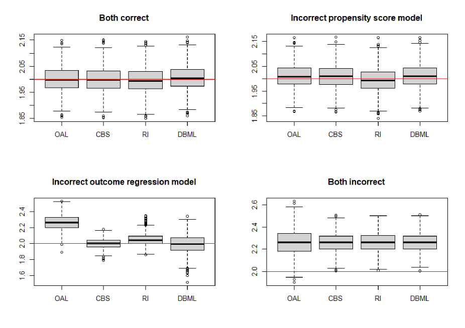
Figure 2: Boxplots of causal effect estimates obtained by $\widehat{\Delta}^{OAL}$, $\widehat{\Delta}^{CBS}$, $\widehat{\Delta}^{RI}$ and $\widehat{\Delta}^{DBML}$. The horizontal red lines correspond to the true causal effect $\Delta=2$. Results are based on 1,000 Monte Carlo runs. This figure appears in color in the electronic version of this article, and any mention of color refers to that version.

6 Real data application

In this session, we analyze data from the Alzheimer’s Disease Neuroimaging Initiative (ADNI) database (adni.loni.usc.edu). The data use acknowledgement is included in the Data Availability Statement Section. We consider the clinical, genetic, and behavioral measures in the ADNI data set. The exposure of interest is the tau protein level in cerebrospinal fluid (CSF) observed at Month 12. Tau is a microtubule-associated protein that promotes microtubule polymerization and stabilization (Kametani and Hasegawa, 2018). Studies (Iqbal et al., 2010) have found that tau protein abnormalities initiate the Alzheimer’s Disease (AD) cascade and cause neurodegeneration and dementia. Under physiological conditions, tau regulates the assembly and maintenance of the structural stability of microtubules. In a diseased brain, however, tau becomes abnormally hyperphosphorylated, which ultimately causes the microtubules to disassemble, and the free tau molecules aggregate into paired helical filaments (Medeiros et al., 2011). Scientists have found that CSF-tau was markedly increased in Alzheimer’s disease (Blennow et al., 2015). In this study, we go beyond association and study whether the CSF-tau protein level affects the severity of the Alzheimer’s Disease.

We dichotomize the CSF-tau protein level using the cutoff value $350$ pg/mL (Tapiola et al., 2009), i.e. $D=1$ if CSF-tau protein level is over $350$ pg/mL, and $D=0$ otherwise. The severity of the AD is measured by the 11-item Alzheimer’s Disease Assessment Scale (ADAS-11) cognitive score observed at Month 24, a widely used measure of cognitive behavior ranging from $0$ to $70$. A higher ADAS-11 score indicates greater severity of AD.

In our analysis, we adjust for clinical and behavioral covariates, including baseline age, gender, and education length, as they are widely considered as the main risk factors for AD (e.g. Guerreiro and Bras, 2015; Vina and Lloret, 2010). We also consider genetic covariates extracted from whole-genome sequencing data from all of the 22 autosomes. We provide details of how we preprocess the genetic data in the Supplementary Material. After pre-processing, $6,087,205$ bi-allelic markers (including SNPs and indels) were retained in the data analysis.

The data set has $268$ subjects with complete information on CSF tau protein data, the Month 24 ADAS-11 score and genetic information. Among these subjects, 82 have CSF-tau protein level above the cut-off point. The mean (SD) age in the high/low tau-protein group is $75.8(7.28)$ and $75.3(6.55)$ years old, respectively, and the mean (SD) education length in the high/low tau-protein group is $15.3(3.05)$ and $15.9(2.99)$ years, respectively. The two groups are unbalanced in terms of gender: 54.9% of study participants in the high tau-protein group are female, while 64.0% of study participants in the low tau-protein group are female. We nevertheless include all three covariates as they were determined a priori. In the Supplementary Material, we report sensitivity analysis in which we adjust for more baseline clinical and behavioral covariates. Analysis results show that adjusting for these additional covariates has minimal effects on the results we obtained.

Denote as $Z$ the covariates age, gender and education length. We first fit a linear regression $Y\sim{Z}$ to adjust for these clinical covariates. We then apply Steps 1-2 of our CBS procedure using the fitted residuals from the linear regression as the outcome and select the top $30$ genetic covariates. We list the top 10 SNPs in Table 2. All of them are located on Chromosome 19 and have previously been found to be strongly associated with Alzheimer’s. See Table S1 in the Supplementary Material for a list of references for the SNPs reported in Table 2.

Table 2: The top ten SNPs selected by Steps 1-2 of our CBS procedure

Rank	SNP name	Gene	Chromosome number
1	rs429358	ApoE	19
2	rs56131196	ApoC1	19
3	rs4420638	ApoC1	19
4	rs12721051	ApoC1	19
5	rs769449	ApoE	19
6	rs10414043	ApoC1	19
7	rs7256200	ApoC1	19
8	rs73052335	ApoC1	19
9	rs111789331	ApoC1	19
10	rs6857	NECTIN2	19

Since some SNPs selected through our first step screening are perfectly correlated, we only keep one among a group of SNPs whose genotypes are identical to each other for the subsequent analysis. We further apply our refined selection procedure in Section 3.2 on these selected covariates and the covariates age, gender and education length, where the coefficients corresponding to the three clinical and behavioral covariates are not penalized. Finally, we use the doubly robust estimator (1) to estimate the average causal effect of CSF-tau protein level on the ADAS-11 score. Analysis results suggest that, on average, being in the high-level CSF-tau group will raise the ADAS-11 score by $5.96$ ($95\%$ CI = $[4.15,7.76]$) points.

In addition to varying the adjusted confounders, in Section 4.3 of the Supplementary Material, we also describe sensitivity analysis varying the number of covariates selected in the first screening step. Tables S2 and S3 suggest that our selection and estimation procedures are relatively robust to the choice of adjusted confounders and the number of covariates selected in the screening step.

7 Discussion

In this paper, we propose a novel selection and estimation procedure for doubly robust causal inference with ultra-high dimensional covariates, called causal ball screening. In comparison to previous approaches that use the same outcome model for propensity score model selection and causal effect estimation, the estimator we propose is doubly robust. Moreover, as we illustrate in the real data analysis, it can be applied to select variables important for causal inference from millions of baseline covariates.

We have so far considered causal effect estimation using the classical doubly robust estimator by Robins et al. (1994). Our developments can also be combined with other techniques for causal effect estimation, such as the covariate balancing propensity score (Imai and Ratkovic, 2014) and the subclassification weights (Wang et al., 2016). This is left as future work.

Data Availability Statement

Data used in preparation of this article were obtained from the Alzheimer’s Disease Neuroimaging Initiative (ADNI) database (http://adni.loni.usc.edu/). As such, the investigators within the ADNI contributed to the design and implementation of ADNI and/or provided data but did not participate in analysis or writing of this report. A complete listing of ADNI investigators can be found at: http://adni.loni.usc.edu/wp-content/uploads/how_to_apply/ADNI_Acknowledgement_List.pdf.

Supporting Information

Web Appendices, Tables, Figures and Proofs referenced in Sections 2, 3, 4 and 6 are available with this paper at the Biometrics website on Wiley Online Library. The proposed CBS method is available both on Wiley Online Library and on Github: https://github.com/dingketang/ultra-high-DRCI.

1 Background for the target adjustment set discussed in Section 2.3

We introduce some definitions we shall use in our paper. A DAG is a finite directed graph with no directed cycles. If a directed edge starts from node $X$ and goes to node $Y$, we say $X$ is a parent of $Y$, and Y is a child of $X$. A directed path is a path trace out entirely along with arrows tail-to-head. If there is a directed path from $X$ to $Y$, then $X$ is an ancestor of $Y$, and $Y$ is a descendant of $X$. Next, we define d-separation (Pearl, 2009).

Definition 5.

(d-separation) A path is blocked by a set of nodes $Z$ if and only if

1. The path contains a chain of nodes $A\rightarrow B\rightarrow C$ or a fork $A\leftarrow B\rightarrow C$ such that the middle node $B$ is in Z (i.e., B is conditioned on), or

2. The path contains a collider $A\rightarrow B\leftarrow C$ such that the collision node $B$ is not in $Z$, and no descendant of $B$ is in $Z$.

If $Z$ blocks every path between two nodes $X$ and $Y$, then $X$ and $Y$ are d-separated conditional on $Z$, otherwise $X$ and $Y$ are d-connected conditional on $Z$.

We introduce some Assumptions under which our definitions of sets have desirable properties.

Assumption 4.

(Causal sufficiency) The causal relationships among $(X,D,Y)$ can be represented by a causal DAG.

Assumption 5.

(Temporal ordering) Every $X_{i}\in X$ is a non-descendant of $D$, which is in turn a non-descendant of $Y$.

Assumption 6.

(Faithfulness) The causal DAG encoding the relationships among $(X,D,Y)$ is faithful. A distribution P is faithful to a DAG $\mathcal{G}$ if no conditional independence relations other than the ones entailed by the Markov property are present.

Proposition 4.

$X^{\mathcal{C}}$, $X^{\mathcal{P}}$, $X^{\mathcal{I}}$, $X^{\mathcal{N}}$ are uniquely defined.

Proposition 5.

For any $\mathcal{S}$ such that $X^{\mathcal{C}}\subset X^{\mathcal{S}}\subset X^{\mathcal{C}}\cup X^{\mathcal{P}}\cup X^{\mathcal{I}}$, assumptions 4 and 5 imply that $D\perp\!\!\!\perp Y(d)\mid X^{\mathcal{S}},d=0,1.$

Proposition 4 shows unicity of our definition. Proposition 5 shows that our definition of confounders satisfies Property 1 proposed by VanderWeele and Shpitser (2013). Under faithfulness, our definition of confounders also satisfies Property 2A of VanderWeele and Shpitser (2013). Proposition 5 is an extension of Propositions 1,2,3,4 in de Luna et al. (2011), the latter imply that $X^{\mathcal{C}}$, $X^{\mathcal{C}}\cup X^{\mathcal{I}}$, $X^{\mathcal{C}}\cup X^{\mathcal{P}}$, $X^{\mathcal{C}}\cup X^{\mathcal{P}}\cup X^{\mathcal{I}}$ are valid adjustment sets.

2 Proofs of Propositions

2.1 Proof of Proposition 4

$pa(Y)$ and $pa(D)$ are uniquely defined by definition. For $X^{(i)}\in pa(Y)$, $X^{(i)}$ and $D$ are either d-connected or not given $pa(Y)\setminus X^{(i)}$. For the first case, $X^{(i)}\in X^{\mathcal{C}}$, and for the second case, $X^{(i)}\in X^{\mathcal{P}}$. Since $pa(D)$ is also uniquely defined, $X^{\mathcal{I}}=pa(D)\setminus X^{\mathcal{C}}$ is uniquely defined.

2.2 Proof of Proposition 5

We first introduce some graphoid axioms (Pearl and Paz, 1985) we will use later:

Intersection: $$D\perp\!\!\!\perp Y\mid W,Z;D\perp\!\!\!\perp W\mid Y,Z\Rightarrow D\perp\!\!\!\perp Y,W\mid Z,$$ (S1)

Contraction: $$D\perp\!\!\!\perp Y\mid Z;D\perp\!\!\!\perp W\mid Y,Z\Rightarrow D\perp\!\!\!\perp Y,W\mid Z,$$ (S2)

Weak union: $$D\perp\!\!\!\perp X\cup Y\mid Z\Rightarrow D\perp\!\!\!\perp X\mid Z\cup Y,$$ (S3)

$$\text{Decomposition}:\quad D\perp\!\!\!\perp X\cup Y\mid Z\Rightarrow D\perp\!\!\!\perp X\mid Z.$$ (S4)

We first show that any superset of $pa(Y)$ is sufficient to adjust for confounding:

$$D\perp\!\!\!\perp Y(d)\mid\bm{X}^{\mathcal{M}},$$ (S5)

where $pa(Y)\subseteq\bm{X}^{\mathcal{M}}$. We show this by contradiction. Assume $D$ and $Y(d)$ are d-connected given $\bm{X}^{\mathcal{M}}$. Due to Assumption 2, there is no direct edge between $D$ and $Y(d)$. Furthermore, $D$ and $Y(d)$ are not ancestral to each other due to Assumptions 5 and 6. Then any path connecting $Y(d)$ and $D$ must be one of the following:

• $Y(d)\leftarrow Q\cdots D$, where $Q$ is a parent of $Y(d).$ Since $Q\in pa(Y)\subset\bm{X}^{\mathcal{M}}$, this path is blocked by $\bm{X}^{\mathcal{M}}$;

• $Y(d)\rightarrow Q\cdots D$. This is impossible since $X^{{(j)}^{\prime}}s$ are non-descendants of $Y(d)$.

We now show that a precision variable is independent of the treatment conditional on confounders (and other precision variables):

$$D\perp\!\!\!\perp\bm{X}^{\tilde{\mathcal{P}}}\mid\{pa(Y)\setminus\bm{X}^{\tilde{\mathcal{P}}}\},$$ (S6)

where $\bm{X}^{\tilde{\mathcal{P}}}=pa(Y)\setminus\bm{X}^{\mathcal{S}}.$

To see this, note that if $j\in\tilde{\mathcal{P}}\subset\mathcal{P}$, by the definition of $\mathcal{P}$ we have $D$ and $X^{(j)}$ are d-separated given $pa(Y)\setminus X^{(j)}$, which implies $D\perp\!\!\!\perp X^{(j)}\mid\{pa(Y)\setminus X^{(j)}\}$. Without loss of generality, assume ${\tilde{\mathcal{P}}}=\{1,2,3,\ldots,d_{0}\}$. We then have

$$\begin{split}&D\perp\!\!\!\perp X^{(1)}\mid[X^{(2)}\cup\{pa(Y)\setminus X^{(1,2)}\}],\\ &D\perp\!\!\!\perp X^{(2)}\mid[X^{(1)}\cup\{pa(Y)\setminus X^{(1,2)}\}].\end{split}$$

By the intersection property (S1), we have $D\perp\!\!\!\perp X^{(1,2)}\mid\{pa(Y)\setminus X^{(1,2)}\}$. Repeat this process $d_{0}-1$ time, we then have $D\perp\!\!\!\perp\bm{X}^{\tilde{\mathcal{P}}}\mid\{pa(Y)\setminus\bm{X}^{\tilde{\mathcal{P}}}\}$.

Combining (S5) and (S6), by the contraction property (S2), we can show that adjusting for all the confounders and any precision variables are sufficient to control for confounding:

$$D\perp\!\!\!\perp Y(d)\mid\{pa(Y)\setminus\bm{X}^{\tilde{\mathcal{P}}}\}.$$

We now show that an instrument variable set is d-separated from, and hence independent of a precision variable conditional on confounders and other precision variables:

$$\bm{X}^{\tilde{\mathcal{I}}}\perp\!\!\!\perp X^{(j)}\mid\{pa(Y)\setminus X^{(j)}\},$$

where ${\tilde{\mathcal{I}}}\subset\mathcal{I}$, $j\in\mathcal{P}$.

We again show by contradiction. Assume there exists $X^{(j)}\in\bm{X}^{\mathcal{P}}$ such that $X^{(j)}$ and $\bm{X}^{\tilde{\mathcal{I}}}$ are d-connected given $pa(Y)\setminus X^{(j)}$. By definition $\bm{X}^{\mathcal{I}}\subset pa(D)$, there is a path $D\leftarrow\bm{X}^{\tilde{\mathcal{I}}}$. Then $D$ and $X^{(j)}$ are d-connected given $pa(Y)\setminus X^{(j)}$, which is a contradiction to the definition of $\mathcal{P}$.

We now show that a set of instruments is independent of any subset of precision variables conditional on confounders and other precision variables:

$$\bm{X}^{\tilde{\mathcal{I}}}\perp\!\!\!\perp\bm{X}^{\tilde{\mathcal{P}}}\mid\{pa(Y)\setminus\bm{X}^{\tilde{\mathcal{P}}}\},$$ (S7)

where $\tilde{\mathcal{I}}\subset\mathcal{I}$. Again, without loss of generality, we assume ${\tilde{\mathcal{P}}}=\{1,2,3,\ldots,d_{0}\}$. We then have:

$$\begin{split}&\bm{X}^{\tilde{\mathcal{I}}}\perp\!\!\!\perp X^{(1)}\mid[X^{(2)}\cup\{pa(Y)\setminus X^{(1,2)}\}],\\ &\bm{X}^{\tilde{\mathcal{I}}}\perp\!\!\!\perp X^{(2)}\mid[X^{(1)}\cup\{pa(Y)\setminus X^{(1,2)}\}].\end{split}$$

By the intersection property (S1), we have $\bm{X}^{\tilde{\mathcal{I}}}\perp\!\!\!\perp X^{(1,2)}\mid\{pa(Y)\setminus X^{(1,2)}\}$. Repeat this process $d_{0}-1$ time, we have $\bm{X}^{\tilde{\mathcal{I}}}\perp\!\!\!\perp\bm{X}^{\tilde{\mathcal{P}}}\mid\{pa(Y)\setminus\bm{X}^{\tilde{\mathcal{P}}}\}$.

Finally, we show

$$D\perp\!\!\!\perp Y(d)\mid\bm{X}^{\mathcal{S}}.$$ (S8)

Using the same argument as in our proof of (S5), we can show that

$$D\perp\!\!\!\perp\bm{X}^{\tilde{\mathcal{P}}}\mid[\bm{X}^{\mathcal{I}}\cup\{pa(Y)\setminus\bm{X}^{\tilde{\mathcal{P}}}\}].$$ (S9)

This relationship holds as $pa(D)\subset\bm{X}^{\mathcal{I}}\cup\{pa(Y)\setminus\bm{X}^{\tilde{\mathcal{P}}}\}$, which means $\bm{X}^{\mathcal{I}}\cup\{pa(Y)\setminus\bm{X}^{\tilde{\mathcal{P}}}\}$ is a superset of $pa(D)$. By letting $\tilde{\mathcal{I}}=\mathcal{I}$ in (S7), combining (S7), (S9) and the contraction property (S2), we have

$$(\bm{X}^{\mathcal{I}}\cup D)\perp\!\!\!\perp\bm{X}^{\tilde{\mathcal{P}}}\mid\{pa(Y)\setminus\bm{X}^{\tilde{\mathcal{P}}}\}.$$ (S10)

Combining (S10) and the decomposition property (S4), for $\tilde{\mathcal{I}}\subset\mathcal{I}$ we have

$$(\bm{X}^{\tilde{\mathcal{I}}}\cup D)\perp\!\!\!\perp\bm{X}^{\tilde{\mathcal{P}}}\mid\{pa(Y)\setminus\bm{X}^{\tilde{\mathcal{P}}}\}.$$

Using the weak union property (S3), we have the following result:

$$D\perp\!\!\!\perp\bm{X}^{\tilde{\mathcal{P}}}\mid[\{pa(Y)\setminus\bm{X}^{\tilde{\mathcal{P}}}\}\cup\bm{X}^{\tilde{\mathcal{I}}}].$$

We set $\tilde{\mathcal{I}}=\mathcal{S}\cap\mathcal{I}\subset\mathcal{I}$. We note that $\{pa(Y)\setminus\bm{X}^{\tilde{\mathcal{P}}}\}\cup(\bm{X}^{\mathcal{S}}\cap\bm{X}^{\mathcal{I}})=[pa(Y)\cap\{pa(Y)\cap(\bm{X}^{\mathcal{S}})^{c}\}^{c}]\cup(\bm{X}^{\mathcal{S}}\cap\bm{X}^{\mathcal{I}})=\{pa(Y)\cap\bm{X}^{\mathcal{S}}\}\cup(\bm{X}^{\mathcal{S}}\cap\bm{X}^{\mathcal{I}})=\bm{X}^{\mathcal{S}}$. The last equality holds because $\mathcal{S}\subset\mathcal{P}\cup\mathcal{I}\cup\mathcal{C}$. So we have

$$D\perp\!\!\!\perp\bm{X}^{\tilde{\mathcal{P}}}\mid\bm{X}^{\mathcal{S}}.$$ (S11)

We let $\mathcal{M}=pa(Y)\cup\mathcal{S}$ in equation (S5). We note that $\bm{X}^{\mathcal{S}}\subset\bm{X}^{\mathcal{M}}$ and $\bm{X}^{\mathcal{S}}\cup\bm{X}^{\tilde{\mathcal{P}}}=\bm{X}^{\mathcal{M}}$. Combining (S11) and (S5), by the contraction property (S2), we have result (S8). $\quad\square$

2.3 Proof of Proposition 3

Under conditions of Lemma 2.1 in (Pan et al., 2018) we have

$$\begin{split}&Bcov(X,Y\mid D)=0\\ \Longleftrightarrow&Bcov(X^{(d)},Y^{(d)})=0,d=0,1\\ \Longleftrightarrow&X^{(d)}\perp\!\!\!\perp Y^{(d)},d=0,1\\ \Longleftrightarrow&X\perp\!\!\!\perp Y\mid D.\end{split}$$

3 Proof of Theorems

3.1 Proof of Theorem 1

Let $\alpha=BCov^{2}(X,Y\mid D)$, $\widehat{\alpha}=BCov_{n}^{2}(X,Y\mid D)$, $\alpha_{1}=BCov^{2}(X^{(1)},Y^{(1)})$ and $\alpha_{0}=BCov^{2}(X^{(0)},Y^{(0)})$, where $(X^{(d)},Y^{(d)})$ follows the same distribution as $(X,Y\mid D=d)$ for $d=0,1$, respectively. We use $\widehat{\alpha}_{1}=BCov^{2}_{n_{1}},(X^{(1)},Y^{(1)})$, $\widehat{\alpha}_{0}=BCov^{2}_{n_{0}}(X^{(0)},Y^{(0)})$ to denote their sample estimators, respectively. To begin with, there exists a constant $\tilde{c}$ such that

$$P(|\alpha-\widehat{\alpha}|>cn^{-k})\leq O_{p}(\exp(-\tilde{c}n^{1-2k})),$$ (S12)

where $c$ and $\kappa$ are defined at condition (A1).

Recall $n_{1}=\sum_{i=1}^{n}D_{i}$, $n_{0}=n-n_{1}$, $\omega=P(D=1)$ and $\widehat{\omega}=n_{1}/n$.

We can write

$$\begin{split}\alpha-\widehat{\alpha}&=\omega\alpha_{1}+(1-\omega)\alpha_{0}-\{\widehat{\omega}\widehat{\alpha}_{1}+(1-\widehat{\omega})\widehat{\alpha}_{0}\}\\ &=\omega(\alpha_{1}-\widehat{\alpha}_{1})+(1-\omega)(\alpha_{0}-\widehat{\alpha}_{0})+(\widehat{\alpha}_{1}-\widehat{\alpha}_{0})(\omega-\widehat{\omega}).\end{split}$$

Since $\alpha_{1},\alpha_{0},\widehat{\alpha}_{1},\widehat{\alpha}_{0}\in[0,1]$, $|\alpha-\widehat{\alpha}|\leq\omega|\alpha_{1}-\widehat{\alpha}_{1}|+(1-\omega)|\alpha_{0}-\widehat{\alpha}_{0}|+|\omega-\widehat{\omega}|$, we have

$$\begin{split}P(|\alpha-\widehat{\alpha}|\geq 2\epsilon)&\leq P(\omega|\alpha_{1}-\widehat{\alpha}_{1}|\geq\omega\epsilon)+P((1-\omega)|\alpha_{0}-\widehat{\alpha}_{0}|\geq(1-\omega)\epsilon)+P(|\omega-\widehat{\omega}|\geq\epsilon)\\ &=P(|\alpha_{1}-\widehat{\alpha}_{1}|\geq\epsilon)+P(|\alpha_{0}-\widehat{\alpha}_{0}|\geq\epsilon)+P(|\omega-\widehat{\omega}|\geq\epsilon).\end{split}$$ (S13)

We control these terms one by one. For the third term of (S13)

$$\omega-\widehat{\omega}=\frac{1}{n}\sum^{n}_{i=1}(\omega-D_{i})=\sum^{n}_{i=1}Z_{i},$$

where $Z_{i}=(\omega-D_{i})/n$ are independent zero-mean random variables, and $|Z_{i}|\leq 1/n=M$, $E(Z_{i}^{2})=\omega(1-\omega)/n^{2}$. Based on the Bernstein inequality, we have

$$P(\omega-\widehat{\omega}\geq\epsilon)=P(\sum^{n}_{i=1}Z_{i}\geq\epsilon)\leq\exp\left(-\frac{\frac{1}{2}\epsilon^{2}}{\frac{\omega(1-\omega)}{n}+\frac{\epsilon}{3n}}\right).$$

So, we have

$$P(|\widehat{\omega}-\omega|\geq\epsilon)=P(\sum^{n}_{i=1}Z_{i}\geq\epsilon)+P(-\sum^{n}_{i=1}Z_{i}\geq\epsilon)\leq 2\exp\left(-\frac{\frac{1}{2}\epsilon^{2}}{\frac{\omega(1-\omega)}{n}+\frac{\epsilon}{3n}}\right).$$ (S14)

Now we control the first and the second terms of (S13). Following equation (A.7) from the appendix of Pan et al. (2018), there exist two positive constants $c_{1}$ and $c_{2}$ such that

$$\begin{split}&P(|\alpha_{1}-\widehat{\alpha}_{1}|\geq\epsilon)\leq 2\exp(-c_{1}n_{1}\epsilon^{2}),\\ &P(|\alpha_{0}-\widehat{\alpha}_{0}|\geq\epsilon)\leq 2\exp(-c_{0}n_{0}\epsilon^{2}).\end{split}$$

We now show that $\exp(-c_{1}n_{1}\epsilon^{2})=O_{p}(\exp(-c_{1}n\omega\epsilon^{2}/2))$. As $\omega=P(D=1)>0$, we have

$$\begin{split}&P\left(\left|\frac{\exp(-c_{1}n_{1}\epsilon^{2})}{\exp(-c_{1}\omega n\epsilon^{2}/2)}\right|>1\right)=P(\frac{n\omega}{2}-n_{1}>0)=P(\omega-\widehat{\omega}>\frac{\omega}{2})\\ &=P(\sum^{n}_{i=1}Z_{i}>\frac{\omega}{2})\leq\exp\left(-\frac{\frac{1}{8}\omega^{2}}{\frac{\omega(1-\omega)}{n}+\frac{\omega}{6n}}\right)\stackrel{{\scriptstyle n\rightarrow\infty}}{{\longrightarrow}}0.\end{split}$$ (S15)

Similarly, we have

$$\exp(-c_{0}n_{0}\epsilon^{2})=O_{p}(\exp(-c_{0}n(1-\omega)\epsilon^{2}/2)).$$ (S16)

When $\epsilon<3\omega(1-\omega)$, we have

$$\exp\left(-\frac{\frac{1}{2}\epsilon^{2}}{\frac{\omega(1-\omega)}{n}+\frac{\epsilon}{3n}}\right)=\exp\left(-\frac{1}{2\omega(1-\omega)+{2\epsilon}/{3}}n\epsilon^{2}\right)\leq\exp(-\tilde{c}_{2}n\epsilon^{2}),$$ (S17)

where $\tilde{c}_{2}=1/\{4\omega(1-\omega)\}$. Let $\epsilon=cn^{-\kappa}/2$, where $0<\kappa<1/2$, $\tilde{c}_{1}=c_{1}\omega/2$, $\tilde{c}_{0}=c_{0}(1-\omega)/2$, combining (S14)–(S17), we have

$$\begin{split}P(|\alpha-\widehat{\alpha}|\geq cn^{-\kappa})&\leq O_{p}(\exp(-\tilde{c}_{1}cn^{1-2\kappa}))+O_{o}(\exp(-\tilde{c}_{0}cn^{1-2\kappa}))\\ &+O_{p}(\exp(-\tilde{c}_{2}cn^{1-2\kappa})).\end{split}$$

Let $\tilde{c}=\min(c\tilde{c}_{1},c\tilde{c}_{0},c\tilde{c}_{2})$, we have

$$\begin{split}P(|\alpha-\widehat{\alpha}|\geq cn^{-\kappa})&\leq O_{p}(\exp(-\tilde{c}n^{1-2\kappa})).\end{split}$$

Hence, we finish the proof of equation (S12). Now let $\rho_{j}=BCov^{2}(X^{(j)},Y\mid D)$ and $\widehat{\rho}_{j}=BCov^{2}_{n}(X^{(j)},Y\mid D)$ for $j=1,2,\ldots,p$. From equation (S12) we know that $P(|\widehat{\rho}_{j}-\rho_{j}|>cn^{-\kappa})=O_{p}(\exp(-c_{1}n^{1-2\kappa}))$.

We then have

$$\begin{split}P(\max_{j\in W}\widehat{\rho}_{j}\geq\min_{j\in\mathcal{A}}\widehat{\rho}_{j})&=P(\max_{j\in W}\widehat{\rho}_{j}-\min_{j\in\mathcal{A}}\rho_{j}\geq\min_{j\in\mathcal{A}}\widehat{\rho}_{j}-\min_{j\in\mathcal{A}}\rho_{j})\\ &=P\{(\max_{j\in W}\widehat{\rho}_{j}-0)-(\min_{j\in\mathcal{A}}\widehat{\rho}_{j}-\min_{j\in\mathcal{A}}\rho_{j})\geq\min_{j\in\mathcal{A}}\rho_{j}\}\\ &\leq P\{(\max_{j\in W}\widehat{\rho}_{j}-0)-(\min_{j\in\mathcal{A}}\widehat{\rho}_{j}-\min_{j\in\mathcal{A}}\rho_{j})\geq 2cn^{-\kappa}\}\\ &\leq P\{(\max_{j\in W}\widehat{\rho}_{j}-0)>cn^{-\kappa}\}+P\{-\min_{j\in\mathcal{A}}\widehat{\rho}_{j}+\min_{j\in\mathcal{A}}\rho_{j}\geq cn^{-\kappa}\}\\ &\leq P\{\max_{j\in W}|\widehat{\rho}_{j}-\rho_{j}|)>cn^{-\kappa}\}+P\{\max_{j\in A}|\widehat{\rho}_{j}-\rho_{j}|)\geq cn^{-\kappa}\}\\ &\leq O(p\exp(-\tilde{c}n^{1-2\kappa})).\end{split}$$

The first inequality holds given condition (A1), and the last inequality holds given equation (S12). Given above results, we have

$$P(\max_{j\in W}\widehat{\rho}_{j}<\min_{j\in\mathcal{A}}\widehat{\rho}_{j})\geq 1-O(p\exp(-\tilde{c}n^{1-2\kappa})).$$

As a result, we have

$$P(\mathcal{A}\subset\widehat{\mathcal{A}})\geq P(\max_{j\in W}\widehat{\rho}_{j}<\min_{j\in\mathcal{A}}\widehat{\rho}_{j})\geq 1-O(p\exp(-\tilde{c}n^{1-2\kappa})).$$

3.2 Proof of Theorem 2

Claims (a) and (b) of Theorem 2 are direct applications of the consistency of Lasso (Zhao and Yu, 2006, Theorem 1) and adaptive Lasso for logistic regression (Shortreed and Ertefaie, 2017, Theorem 1) respectively. We now show claims (c) and (d).

We first show the following results:

1. If (6) holds and $\widehat{\mathcal{A}}_{OR}=\mathcal{A},$ then $\frac{1}{n}\sum^{n}_{i=1}\{b_{d}(X_{i},\widehat{\alpha}^{(d)})-b_{d}^{0}(X_{i},\alpha^{(d)})\}^{2}=O_{p}(1/n^{2/3})$;

2. If (7) holds and $\widehat{\mathcal{A}}_{PS}=\mathcal{A},$ then $\frac{1}{n}\sum^{n}_{i=1}\{e(X_{i},\widehat{\beta})-e^{0}(X_{i},\beta)\}^{2}=O_{p}(1/n)$.

Proof of (i):

$$\begin{split}\frac{1}{n}\sum^{n}_{i=1}\{b_{d}(X_{i},\widehat{\alpha}^{(d)})-b_{d}(X_{i},\alpha^{(d)*})\}^{2}&=\frac{1}{n}\sum^{n}_{i=1}\{X_{i,\mathcal{A}}^{\mathrm{\scriptscriptstyle T}}(\widehat{\alpha}^{(d)}_{\mathcal{A}}-{\alpha}^{(d)*}_{\mathcal{A}})\}^{2}\\ &=(\widehat{\alpha}^{(d)}_{\mathcal{A}}-{\alpha}^{(d)*}_{\mathcal{A}})^{\mathrm{\scriptscriptstyle T}}(\frac{1}{n}X_{\mathcal{A}}^{\mathrm{\scriptscriptstyle T}}X_{\mathcal{A}})(\widehat{\alpha}^{(d)}_{\mathcal{A}}-{\alpha}^{(d)*}_{\mathcal{A}})\\ &\leq O_{p}(\frac{1}{n^{2/3}}).\end{split}$$

The last inequality holds because $(\frac{1}{n}X_{\mathcal{A}}^{\mathrm{\scriptscriptstyle T}}X_{\mathcal{A}})\overset{p}{\longrightarrow}C$ given condition (B4), and $(\widehat{\alpha}^{(d)}_{\mathcal{A}}-{\alpha}^{(d)*}_{\mathcal{A}})\leq O_{p}(\lambda^{(d)}_{Y}/n)$ given lemma 3 in Zou (2006).

Proof of (ii):

$$\begin{split}\frac{1}{n}\sum^{n}_{i=1}\{e(X_{i},\widehat{\beta})-e(X_{i})\}^{2}&=\frac{1}{n}\sum^{n}_{i=1}\{\text{expit}(X_{i,\mathcal{A}}^{\mathrm{\scriptscriptstyle T}}\widehat{\beta}_{\mathcal{A}})-\text{expit}(X_{i,\mathcal{A}}^{\mathrm{\scriptscriptstyle T}}\beta^{*}_{\mathcal{A}})\}^{2}\\ &\leq\frac{1}{n}\sum^{n}_{i=1}\{X_{i,\mathcal{A}}^{\mathrm{\scriptscriptstyle T}}\widehat{\beta}_{\mathcal{A}}-X_{i,\mathcal{A}}^{\mathrm{\scriptscriptstyle T}}\beta^{*}_{\mathcal{A}}\}^{2}\\ &=(\widehat{\beta}_{\mathcal{A}}-{\beta}^{*}_{\mathcal{A}})^{\mathrm{\scriptscriptstyle T}}(\frac{1}{n}X_{\mathcal{A}}^{\mathrm{\scriptscriptstyle T}}X_{\mathcal{A}})(\widehat{\beta}_{\mathcal{A}}-{\beta}^{*}_{\mathcal{A}})\\ &\leq O_{p}(1/n).\end{split}$$

The last inequality holds because $(\frac{1}{n}X_{\mathcal{A}}^{\mathrm{\scriptscriptstyle T}}X_{\mathcal{A}})\overset{p}{\longrightarrow}C$ given condition (B4), and $(\widehat{\beta}_{\mathcal{A}}-{\beta}^{*}_{\mathcal{A}})\leq O_{p}(1/\sqrt{n})$ given Shortreed and Ertefaie (2017, Theorem 2(b)).

Proof of Claim (c):

We have the following decomposition:

$$\begin{split}\widehat{\Delta}-\Delta&=\frac{1}{n}\sum^{n}_{i=1}\phi(Y_{i},b^{0}_{1}(X_{i}),b^{0}_{0}(X_{i}),e^{0}(X_{i}),D_{i},\Delta)+R_{1}+R_{2}+R_{3}+R_{4},\end{split}$$

where

$$\begin{split}R_{1}&=\frac{1}{n}\sum^{n}_{i=1}\{b_{1}(X_{i},\widehat{\alpha}^{(1)})-b_{1}^{0}(X_{i})\}-\frac{1}{n}\sum^{n}_{i=1}\{b_{0}(X_{i},\widehat{\alpha}^{(0)})-b_{0}^{0}(X_{i})\},\\ R_{2}&=\frac{1}{n}\sum^{n}_{i=1}\frac{D_{i}Y_{i}}{{e(X_{i},\widehat{\beta})e^{0}(X_{i})}}\{e^{0}(X_{i})-e(X_{i},\widehat{\beta})\}\\ &+\frac{1}{n}\sum^{n}_{i=1}\frac{(1-D_{i})Y_{i}}{\{1-e(X_{i},\widehat{\beta})\}\{1-e^{0}(X_{i})\}}\{e^{0}(X_{i})-e(X_{i},\widehat{\beta})\},\\ R_{3}&=-\frac{1}{n}\sum^{n}_{i=1}\frac{D_{i}}{e(X_{i},\widehat{\beta})}\{b_{1}(X_{i},\widehat{\alpha}^{(1)})-b_{1}^{0}(X_{i})\}+\frac{1}{n}\sum^{n}_{i=1}\frac{1-D_{i}}{1-e(X_{i},\widehat{\beta})}\{b_{0}(X_{i},\widehat{\alpha}^{(0)})-b_{0}^{0}(X_{i})\},\\ R_{4}&=\frac{1}{n}\sum^{n}_{i=1}\frac{D_{i}b_{1}^{0}(X_{i})}{e(X_{i},\widehat{\beta})e^{0}(X_{i})}\{e(X_{i},\widehat{\beta})-e^{0}(X_{i})\}\\ &+\frac{1}{n}\sum^{n}_{i=1}\frac{(1-D_{i})b_{0}^{0}(X_{i})}{\{1-e(X_{i},\widehat{\beta})\}\{1-e^{0}(X_{i})\}}\{e(X_{i},\widehat{\beta})-e^{0}(X_{i})\}.\end{split}$$

Under Assumption 3, the Cauchy-Schwarz inequality and the consistency condition of Theorem 3.2 (c), $R_{1}$, $R_{2}$, $R_{3}$, $R_{4}$ are $o_{p}(1)$.

$$\frac{1}{n}\sum^{n}_{i=1}\phi(Y_{i},b^{0}_{1}(X_{i}),b^{0}_{0}(X_{i}),e^{0}(X_{i}),D_{i},\Delta)\overset{p}{\longrightarrow}\Delta$$

if $b^{0}_{d}(X_{i})=b_{d}(X_{i},\alpha^{(d)^{*}})$ or $e^{0}(X_{i})=e(X_{i},\beta^{*})$, which holds by claim (i) and (ii).

Proof of Claim (d):

We have the following decomposition:

$$\begin{split}\sqrt{n}(\widehat{\Delta}-\Delta)-\sum^{n}_{i=1}\{\phi(Y_{i},b_{1}(X_{i,\mathcal{A}}),b_{0}(X_{i,\mathcal{A}}),e(X_{i,\mathcal{A}}),D_{i},\Delta)\}/\sqrt{n}=R_{1}+R_{21}+R_{22},\end{split}$$

where

$$\begin{split}R_{1}&=\frac{1}{\sqrt{n}}\sum^{n}_{i=1}D_{i}\{Y_{i}-b_{1}(X_{i},\alpha^{(1)*})\}\{\frac{1}{e(X_{i},\widehat{\beta})}-\frac{1}{e(X_{i},\beta^{*})}\}\\ &-\frac{1}{\sqrt{n}}\sum^{n}_{i=1}(1-D_{i})\{Y_{i}-b_{0}(X_{i},\alpha^{(0)*})\}\{\frac{1}{1-e(X_{i},\widehat{\beta})}-\frac{1}{1-e(X_{i},\beta^{*})}\},\\ R_{21}&=\frac{1}{\sqrt{n}}\sum^{n}_{i=1}\left[\{b_{1}(X_{i},\widehat{\alpha}^{(1)})-b_{1}(X_{i},\alpha^{(1)*})\}\frac{e(X_{i},\beta^{*})-D_{i}}{e(X_{i},\beta^{*})}\right]\\ &+\frac{1}{\sqrt{n}}\sum^{n}_{i=1}\left[\{b_{0}(X_{i},\widehat{\alpha}^{(1)})-b_{0}(X_{i},\alpha^{(1)*})\}\frac{e(X_{i},\beta^{*})-D_{i}}{e(X_{i},\beta^{*})}\right],\\ R_{22}&=\frac{1}{\sqrt{n}}\sum^{n}_{i=1}\left[\{b_{1}(X_{i},\widehat{\alpha}^{(1)})-b_{1}(X_{i},\alpha^{(1)*})\}\{e(X_{i},\widehat{\beta})-e(X_{i},\beta^{*})\}\frac{D_{i}}{e(X_{i},\widehat{\beta})e(X_{i},\beta^{*})}\right]\\ +&\frac{1}{\sqrt{n}}\sum^{n}_{i=1}\left[\{b_{0}(X_{i},\widehat{\alpha}^{(1)})-b_{0}(X_{i},\alpha^{(1)*})\}\{e(X_{i},\widehat{\beta})-e(X_{i},\beta^{*})\}\frac{1-D_{i}}{(1-e(X_{i},\widehat{\beta}))(1-e(X_{i},\beta^{*}))}\right].\end{split}$$

Due to symmetry, we only show that the first term of $R_{1},\;R_{21},\;R_{22}$ are $o_{p}(1)$ using (i) and (ii).

For $R_{1}$, let the first and second term of $R_{1}$ be $R_{11}$ and $R_{12}$, respectively. We have

$$\begin{split}\mathbb{E}(R_{11}^{2}\mid\{X_{i},D_{i}\}^{n}_{i=1})=&\frac{1}{n}\sum^{n}_{i=1}\frac{D_{i}\sigma^{2}}{e^{2}(X_{i},\beta^{*})e^{2}(X_{i},\widehat{\beta})}\{e(X_{i},\widehat{\beta})-e(X_{i},\widehat{\beta}^{*})\}^{2}\\ \leq&\frac{C}{n}\sum^{n}_{i=1}\{e(X_{i},\widehat{\beta})-e(X_{i},\widehat{\beta}^{*})\}^{2}\\ \leq&o_{p}(1).\end{split}$$

Because $\mathbb{E}(R_{11}\mid\{X_{i},D_{i}\}^{n}_{i=1})=0$, we have $R_{11}=o_{p}(1)$.

Similarly, let the first and second term of $R_{21}$ be $R_{211}$ and $R_{212}$, respectively. We have

$$\begin{split}\mathbb{E}(R_{211}^{2}\mid\{X_{i},D_{i}\}^{n}_{i=1})&=\frac{1}{n}\sum^{n}_{i=1}\left[\{b_{1}(X_{i},\widehat{\alpha}^{(1)})-b_{1}(X_{i},\alpha^{(1)*})\}^{2}\left\{\frac{e(X_{i},\beta^{*})-D_{i}}{e(X_{i},\beta^{*})}\right\}^{2}\right]\\ &\leq\frac{C}{n}\sum^{n}_{i=1}\{b_{1}(X_{i},\widehat{\alpha}^{(1)})-b_{1}(X_{i},\alpha^{(1)*})\}^{2}\\ &\leq o_{p}(1).\end{split}$$

By the same argument as $R_{11}$, we can show that $R_{211}$ is $o_{p}(1)$.

For $R_{22}$, by the Cauchy-Schwarz inequality,

$$\begin{split}&\frac{1}{\sqrt{n}}\sum^{n}_{i=1}\left[\{b_{1}(X_{i},\widehat{\alpha}^{(1)})-b_{1}(X_{i},\alpha^{(1)*})\}\{e(X_{i},\widehat{\beta})-e(X_{i},\beta^{*})\}\frac{D_{i}}{e(X_{i},\widehat{\beta})e(X_{i},\beta^{*})}\right]\\ \leq&\frac{1}{\sqrt{n}}\max\{e(X_{i},\widehat{\beta})e(X_{i},\beta^{*})\}\sqrt{\sum^{n}_{i=1}\{b_{1}(X_{i},\widehat{\alpha}^{(1)})-b_{1}(X_{i},\alpha^{(1)*})\}^{2}\sum^{n}_{i=1}\{e(X_{i},\widehat{\beta})-e(X_{i},\beta^{*})\}^{2}}\\ \leq&O_{p}(\frac{1}{\sqrt{n}})O_{p}(1)O_{p}(n^{1/6})\\ \leq&o_{p}(1).\end{split}$$

Hence, we have finished the proof of Theorem 2 (d.1). For Theorem 2 (d.3), the proof is very similar to the ones in the proof of Theorem 3.3 in Farrell (2015). Proofs for the remaining parts of Theorem 2 are straightforward and hence omitted.

4 Additional real data results

4.1 Genetics data preprocessing

For these genetic data, we applied the following preprocessing technique. The first line quality control steps include (i) call rate check per subject and per Single Nucleotide Polymorphism (SNP) marker, (ii) gender check, (iii) sibling pair identification, (iv) the Hardy-Weinberg equilibrium test, (v) marker removal by the minor allele frequency, and (vi) population stratification. The second line preprocessing steps include removal of SNPs with (i) more than 5$\%$ missing values, (ii) minor allele frequency (MAF) smaller than 10$\%$, and (iii) Hardy-Weinberg equilibrium p-value $<10^{-6}$. $503,892$ SNPs obtained from 22 chromosomes were included in for further processing. MACH-Admix software (http://www.unc.edu/ yunmli/MaCH-Admix/) (Liu et al., 2013) is applied to perform genotype imputation, using 1000G Phase I Integrated Release Version 3 haplotypes (http://www.1000genomes.org) (1000 Genomes Project Consortium, 2012) as a reference panel. Quality control was also conducted after imputation, excluding markers with (i) low imputation accuracy (based on imputation output $R^{2}$), (ii) Hardy-Weinberg equilibrium p-value $10^{-6}$, and (iii) minor allele frequency (MAF) $<5\%$.

4.2 Related literature for the top 10 SNPs listed in Table 2

In Table S1, we include references for the top 10 listed in Table 2.

Table S1: The top ten SNPs selected by our CBS procedure

Rank	SNP name	Gene	Chromosome number	Related references
1	rs429358	ApoE	19	Cramer et al. (2012)
2	rs56131196	ApoC1	19	Guerreiro et al. (2012)
3	rs4420638	ApoC1	19	Guerreiro et al. (2012)
4	rs12721051	ApoC1	19	Gao et al. (2016)
5	rs769449	ApoE	19	Cruchaga et al. (2013)
6	rs10414043	ApoC1	19	Zhou et al. (2014)
7	rs7256200	ApoC1	19	Takei et al. (2009)
8	rs73052335	ApoC1	19	Zhou et al. (2014)
9	rs111789331	ApoC1	19	Rajabli et al. (2018)
10	rs6857	NECTIN2	19	Kamboh et al. (2012)

4.3 Sensitivity analysis

We perform sensitivity analysis by varying the number of observed confounders adjusted and the number of covariates kept in the first screening step. In the analyses reported in Section 6 of the main paper, we adjust for the observed confounders baseline age, gender, and education length as they are the main risk factors for AD (Guerreiro and Bras, 2015; Vina and Lloret, 2010). In the dataset, there are other covariates available including handedness, retirement status, and martial status. In the sensitivity analysis, we adjust for these additional covariates in addition to the age, gender, and education length. We also perform another set of sensitivity analyses by setting a different threshold for the cardinality of set $\mathcal{K}$ selected by the first screening step. In addition to the number $30$ used in the main paper, we also consider $q=40$ ,$50$, or $\lfloor n/\log(n)\rfloor=47$, the last of which was suggested by Fan and Lv (2008). The results are included in Table S2. The estimated average causal effects are similar in all settings.

Table S2: The top ten SNPs selected by our CBS procedure with additional clinical confounders

Rank	SNP name	Gene	Chromosome number	Related references	Rank in the old procedure
1	rs429358	ApoE	19	Cramer et al. (2012)	1
2	rs12721051	ApoC1	19	Gao et al. (2016)	4
3	rs56131196	ApoC1	19	Guerreiro et al. (2012)	2
4	rs4420638	ApoC1	19	Guerreiro et al. (2012)	3
5	rs769449	ApoE	19	Cruchaga et al. (2013)	5
6	rs10414043	ApoC1	19	Zhou et al. (2014)	6
7	rs7256200	ApoC1	19	Takei et al. (2009)	7
8	rs73052335	ApoC1	19	Zhou et al. (2014)	8
9	rs111789331	ApoC1	19	Rajabli et al. (2018)	9
10	rs6857	NECTIN2	19	Kamboh et al. (2012)	10

Table S2 shows the top 10 SNPs from the screening step with additional clinical confounders. One can see immediately that Table S2 is quite similar to Table S1. We get the same SNPs with different orders. Table S3 provides point estimates and confidence intervals with different clinical confounders and thresholds for the cardinality of $|\mathcal{K}|$. These estimates are close to each other, suggesting that our method is relatively robust to the clinical/behavioral confounders we adjust for, and the number of covariates we keep in the screening step.

Table S3: Point estimates and 95% confidence interval with different clinical/behavioral covariates and cardinality of $\mathcal{K}$

Clinical confounders	Threshold $|\mathcal{K}|$	Point estimate	95% confidence interval
age,gender, education length	30	5.96	[4.15, 7.76]
	40	5.95	[4.25, 7.64]
	50	6.08	[4.25, 7.91]
	47$(\lfloor n/\log(n)\rfloor)$	6.08	[4.30, 7.90]
age,gender, education length, handedness, retirement status, marital status	30	6.68	[4.96, 8.40]
	40	6.76	[5.09, 8.43]
	50	6.75	[5.06, 8.44]
	47$(\lfloor n/\log(n)\rfloor)$	6.76	[5.05, 8.48]

References

- 1000 Genomes Project Consortium (2012) 1000 Genomes Project Consortium (2012). An integrated map of genetic variation from 1,092 human genomes. Nature 491, 56–65.
- Antonelli et al. (2019) Antonelli, J., Parmigiani, G., and Dominici, F. (2019). High-dimensional confounding adjustment using continuous spike and slab priors. Bayesian Analysis 14, 825–848.
- Barut et al. (2016) Barut, E., Fan, J., and Verhasselt, A. (2016). Conditional sure independence screening. Journal of the American Statistical Association 111, 1266–1277.
- Berrett et al. (2019) Berrett, T. B., Samworth, R. J., and Yuan, M. (2019). Efficient multivariate entropy estimation via -nearest neighbour distances. The Annals of Statistics 47, 288–318.
- Blennow et al. (2015) Blennow, K., Dubois, B., Fagan, A. M., Lewczuk, P., de Leon, M. J., and Hampel, H. (2015). Clinical utility of cerebrospinal fluid biomarkers in the diagnosis of early Alzheimer’s disease. Alzheimer’s & Dementia 11, 58–69.
- Brookhart et al. (2006) Brookhart, M. A., Schneeweiss, S., Rothman, K. J., Glynn, R. J., Avorn, J., and Stürmer, T. (2006). Variable selection for propensity score models. American Journal of Epidemiology 163, 1149–1156.
- Chernozhukov et al. (2018) Chernozhukov, V., Chetverikov, D., Demirer, M., Duflo, E., Hansen, C., Newey, W., et al. (2018). Double/debiased machine learning for treatment and structural parameters. The Econometrics Journal 21, C1–C68.
- Cover and Thomas (2012) Cover, T. M. and Thomas, J. A. (2012). Elements of information theory. John Wiley & Sons.
- Cramer et al. (2012) Cramer, P. E., Cirrito, J. R., Wesson, D. W., Lee, C. D., Karlo, J. C., Zinn, A. E., et al. (2012). Apoe-directed therapeutics rapidly clear -amyloid and reverse deficits in ad mouse models. Science 335, 1503–1506.
- Cruchaga et al. (2013) Cruchaga, C., Kauwe, J. S., Harari, O., Jin, S. C., Cai, Y., Karch, C. M., et al. (2013). Gwas of cerebrospinal fluid tau levels identifies risk variants for Alzheimer’s disease. Neuron 78, 256–268.
- de Luna et al. (2011) de Luna, X., Waernbaum, I., and Richardson, T. S. (2011). Covariate selection for the nonparametric estimation of an average treatment effect. Biometrika 98, 861–875.
- Ding and Miratrix (2015) Ding, P. and Miratrix, L. W. (2015). To adjust or not to adjust? Sensitivity analysis of M-bias and butterfly-bias. Journal of Causal Inference 3, 41–57.
- Ertefaie et al. (2018) Ertefaie, A., Asgharian, M., and Stephens, D. A. (2018). Variable selection in causal inference using a simultaneous penalization method. Journal of Causal Inference 6, 20170010.
- Fan and Lv (2008) Fan, J. and Lv, J. (2008). Sure independence screening for ultrahigh dimensional feature space. Journal of the Royal Statistical Society: Series B (Statistical Methodology) 70, 849–911.
- Farrell (2015) Farrell, M. H. (2015). Robust inference on average treatment effects with possibly more covariates than observations. Journal of Econometrics 189, 1–23.
- Gao et al. (2016) Gao, L., Cui, Z., Shen, L., and Ji, H.-F. (2016). Shared genetic etiology between type 2 diabetes and Alzheimer’s disease identified by bioinformatics analysis. Journal of Alzheimer’s Disease 50, 13–17.
- Guerreiro and Bras (2015) Guerreiro, R. and Bras, J. (2015). The age factor in Alzheimer’s disease. Genome Medicine 7, 106.
- Guerreiro et al. (2012) Guerreiro, R. J., Gustafson, D. R., and Hardy, J. (2012). The genetic architecture of Alzheimer’s disease: beyond app, psens and apoe. Neurobiology of Aging 33, 437–456.
- Hahn (1998) Hahn, J. (1998). On the role of the propensity score in efficient semiparametric estimation of average treatment effects. Econometrica 66, 315–331.
- Hahn (2004) Hahn, J. (2004). Functional restriction and efficiency in causal inference. Review of Economics and Statistics 86, 73–76.
- Imai and Ratkovic (2014) Imai, K. and Ratkovic, M. (2014). Covariate balancing propensity score. Journal of the Royal Statistical Society: Series B (Statistical Methodology) 76, 243–263.
- Iqbal et al. (2010) Iqbal, K., Liu, F., Gong, C.-X., and Grundke-Iqbal, I. (2010). Tau in Alzheimer disease and related tauopathies. Current Alzheimer Research 7, 656–664.
- Kamboh et al. (2012) Kamboh, M. I., Barmada, M. M., Demirci, F. Y., Minster, R. L., Carrasquillo, M. M., Pankratz, V. S., et al. (2012). Genome-wide association analysis of age-at-onset in Alzheimer’s disease. Molecular Psychiatry 17, 1340–1346.
- Kametani and Hasegawa (2018) Kametani, F. and Hasegawa, M. (2018). Reconsideration of amyloid hypothesis and tau hypothesis in Alzheimer’s disease. Frontiers in Neuroscience 12, 25.
- Leeb and Pötscher (2005) Leeb, H. and Pötscher, B. M. (2005). Model selection and inference: Facts and fiction. Econometric Theory 21, 21–59.
- Liu et al. (2013) Liu, E., Li, M., Wang, W., and Li, Y. (2013). Mach-admix: Genotype imputation for admixed populations. Genetic Epidemiology 37, 25–37.
- Liu et al. (2012) Liu, W., Brookhart, M. A., Schneeweiss, S., Mi, X., and Setoguchi, S. (2012). Implications of M bias in epidemiologic studies: A simulation study. American Journal of Epidemiology 176, 938–948.
- Medeiros et al. (2011) Medeiros, R., Baglietto-Vargas, D., and LaFerla, F. M. (2011). The role of tau in Alzheimer’s disease and related disorders. CNS Neuroscience & Therapeutics 17, 514–524.
- Moosavi et al. (2021) Moosavi, N., Häggström, J., and de Luna, X. (2021). The costs and benefits of uniformly valid causal inference with high-dimensional nuisance parameters. https://arxiv.org/abs/2105.02071.
- Pan et al. (2018) Pan, W., Tian, Y., Wang, X., and Zhang, H. (2018). Ball divergence: nonparametric two sample test. The Annals of Statistics 46, 1109–1137.
- Pan et al. (2018) Pan, W., Wang, X., Xiao, W., and Zhu, H. (2018). A generic sure independence screening procedure. Journal of the American Statistical Association 114, 928–937.
- Pan et al. (2020) Pan, W., Wang, X., Zhang, H., Zhu, H., and Zhu, J. (2020). Ball covariance: A generic measure of dependence in Banach space. Journal of the American Statistical Association 115, 307–317.
- Pearl (2009) Pearl, J. (2009). Causality. Cambridge University Press.
- Pearl and Paz (1985) Pearl, J. and Paz, A. (1985). Graphoids: A graph-based logic for reasoning about relevance relations. University of California (Los Angeles). Computer Science Department.
- Rajabli et al. (2018) Rajabli, F., Feliciano, B. E., Celis, K., Hamilton-Nelson, K. L., Whitehead, P. L., Adams, L. D., et al. (2018). Ancestral origin of ApoE 4 Alzheimer’s disease risk in puerto rican and african american populations. PLoS Genetics 14, e1007791.
- Robins et al. (1994) Robins, J. M., Rotnitzky, A., and Zhao, L. P. (1994). Estimation of regression coefficients when some regressors are not always observed. Journal of the American Statistical Association 89, 846–866.