Nonnegative Low Rank Tensor Approximation with Applications to Multi-dimensional Images

Abstract

The main aim of this paper is to develop a new algorithm for computing nonnegative low rank tensor approximation for nonnegative tensors that arise in many multi-dimensional imaging applications. Nonnegativity is one of the important property as each pixel value refers to nonzero light intensity in image data acquisition. Our approach is different from classical nonnegative tensor factorization (NTF) which requires each factorized matrix and/or tensor to be nonnegative. In this paper, we determine a nonnegative low Tucker rank tensor to approximate a given nonnegative tensor. We propose an alternating projections algorithm for computing such nonnegative low rank tensor approximation, which is referred to as NLRT. The convergence of the proposed manifold projection method is established. Experimental results for synthetic data and multi-dimensional images are presented to demonstrate the performance of NLRT is better than state-of-the-art NTF methods.

1 Introduction

Nonnegative data is very common in many data analysis applications. For instance, in image analysis, image pixel values are nonnegative and the associated images can be seen as nonnegative matrices for clustering and recognition tasks. When the data is already high dimensional by nature, for example, video data, hyperspectral data, fMRI data and so on, it then seems more natural to represent the information in a high dimensional space, rather than flatten the data to a matrix. The data represented in high dimension is referred to as a tensor.

An $m$-dimensional tensor $\mathcal{A}$ is a multi-dimensional array, $\mathcal{A}\in\mathbb{R}^{n_{1}\times\cdots\times n_{m}}$. To extract pertinent information from a given large tensor data, low rank tensor decompositions are usually considered. In recent decades, various of tensor decompositions have been developed according to different applications. The most famous and widely used decompositions are Canonical Polyadic decomposition (CPD) and Tucker decomposition. For more details of tensor applications and tensor decompositions, we refer to the review papers kolda2009tensor ; sidiropoulos2017tensor . In this paper, we only target on tensor in a Tucker form. Hence, in the following, we will briefly review Tucker decomposition.

Given a tensor $\mathcal{A}\in\mathbb{R}^{n_{1}\times n_{2}\times\cdots\times n_{m}}$, the Tucker decomposition de2000multilinear ; tucker1966some ; kolda2009tensor is defined as follows:

$$\mathcal{A}=\mathcal{G}\times_{1}\mathbf{U}^{(1)}\times_{2}\mathbf{U}^{(2)}\times_{3}\cdots\times_{m}\mathbf{U}^{(m)},$$ (1)

i.e.,

$${\cal A}_{i_{1},\cdots,i_{m}}=\sum_{j_{1},\cdots,j_{m}}{\cal G}_{j_{1},\cdots,j_{m}}{\bf U}^{(1)}_{i_{1},j_{1}}\cdots{\bf U}^{(m)}_{i_{m},j_{m}},$$ (2)

where $\mathcal{G}=({\cal G}_{j_{1},j_{2},\cdots,j_{m}})\in\mathbb{R}^{J_{1}\times J_{2}\times\cdots\times J_{m}}$, ${\bf U}^{(k)}$ is a $n_{k}$-by-$J_{k}$ matrix (whose columns are usually mutually orthogonal), $\times_{k}$ denotes the $k$-mode matrix product of a tensor defined by

$$(\mathcal{G}\times_{k}\mathbf{U}^{(k)})_{j_{1}\cdots j_{k-1}i_{k}j_{k+1}\cdots j_{m}}=\sum^{J_{k}}_{j_{k}=1}{\cal G}_{j_{1}\cdots j_{k-1}j_{k}j_{k+1}\cdots j_{m}}{\bf U}^{(k)}_{i_{k},j_{k}}.$$

The minimal value of $(J_{1},J_{2},\cdots,J_{m})$ is defined as Tucker (or multilinear) rank of ${\cal A}$, denoted as $\operatorname{rank}_{T}({\cal A})=(J_{1},J_{2},\cdots,J_{m})$.

Since high-dimensional nonnegative data are everywhere in real world, and the nonnegativity of factor matrices derived from the tensor decompositions can lead to interpretations for real applications, many nonnegative tensor decompositions have been proposed and developed, and most of them are based on tensor decomposition with nonnegative constraints. For Tucker decomposition with nonnegative constraints, that is referred to as Nonnegative Tucker Decomposition (NTD) in kim2007nonnegative , aims to solve

$$\begin{split}&\min\|\mathcal{A}-\mathcal{X}\|\\ &\mbox{s.t.}\quad\mathcal{X}=\mathcal{S}\times_{1}\mathbf{P}_{1}\times_{2}\mathbf{P}_{2}\times_{3}\cdots\times_{m}\mathbf{P}_{m},\\ &\quad\quad\mathcal{S}\in\mathbb{R}^{r_{1}\times\cdots\times r_{m}}_{+},\quad\mathbf{P}_{k}\in\mathbb{R}^{n_{k}\times r_{k}}_{+},\quad k=1,\cdots m.\end{split}$$ (3)

In kim2007nonnegative , Kim and Choi first studied this model and proposed multiplicative updating algorithms extended from nonnegative matrix factorization (NMF) to solve it. In zhou2012fast , Zhou et al. transformed this problem into a series of NMF problem, and used MU and HALS algorithms on the unfolding matrices for Tucker decomposition calculation. Some other constraints like orthogonality on the factor matrices are also considered and studied by some researchers xutaoli2017 ; pan2019orthogonal . For instance, in pan2019orthogonal , Pan et al. proposed orthogonal nonnegative Tucker decomposition and applied the alternating direction method of multipliers (ADMM), to get clustering informations from the factor matrices and the joint connection weight from the core tensor.

The biggest advantage of NTD model is the core tensor and factor matrices can be interpretable thanks to the requirement of the factorized components. However the approximation $\mathcal{X}$ is not the best approximation of $\mathcal{A}$ for the given Tucker rank $(r_{1},\cdots,r_{m})$. Hence it is required to find the best low Tucker rank nonnegative approximation for a given nennegative tensor $\mathcal{A}$ with interpretable factor matrices and core tensor. In this paper, we propose the following problem. Given tensor $\mathcal{A}\in\mathbb{R}^{n_{1}\times\cdots\times n_{m}}_{+}$,

$$\min_{\mathcal{X}\geq 0}\|{\cal A}-{\cal X}\|_{F}^{2},\quad\mbox{s.t.}\quad rank_{T}(\mathcal{X})=(r_{1},r_{2},\cdots,r_{m}).$$ (4)

From $rank_{T}(\mathcal{X})=(r_{1},r_{2},\cdots,r_{m})$, we can deduce that there exist core tensor ${\cal S}\in\mathbb{R}^{r_{1}\times r_{2}\times\cdots\times r_{m}}$ and orthogonal factor matrices $\{{\bf P}_{k}:{\bf P}_{k}\in\mathbb{R}^{n_{k}\times r_{k}},{\bf P}^{T}_{k}{\bf P}_{k}=\mathbf{I}_{r_{k}},k=1,\cdots,m\}$, such that

$${\cal X}={\cal S}\times_{1}{\bf P}_{1}\times_{2}{\bf P}_{2}\times_{3}\cdots\times_{m}{\bf P}_{m}.$$

For $k=1,\cdots,m$, let $\mathbf{X}_{k}$ be the $k$-th unfolding of tensor $\mathcal{X}$, defined as $\mathbf{X}_{k}\in\mathbb{R}^{n_{k}\times(n_{k+1}\cdots n_{m}n_{1}\cdots n_{k-1})}$. From the definition of Tucker decomposition, we deduce that $r_{k}=rank(\mathbf{X}_{k})$, and factor matrix $\mathbf{P}_{k}$ can be obtained by singular value decomposition on ${\bf X}_{k}$:

$${\bf X}_{k}={\bf P}_{k}{\bf\Sigma}_{k}{\bf Q}_{k}^{T},$$

here ${\bf\Sigma}_{k}$ is a diagonal matrix of size $r_{k}$-by-$r_{k}$, and ${\bf Q}_{k}$ is $n_{k}$-by-$r_{k}$ with orthonormal columns (${\bf Q}_{k}^{T}$ is the transpose of ${\bf Q}_{k}$).

We remark that problem (4) without the nonnegativity constraint on the approximation $\mathcal{X}$ is referred to as the best low multilinear rank approximation problem, which has been well discussed and used widely as a tool in dimensionality reduction and signal subspace estimation in recent two decades. The classical methods for the problem are truncated higher-order SVD (HOSVD)de2000multilinear and higher-order orthogonal iteration (HOOI) de2000best ; kroonenberg2008applied , proposed based on a higher-order extension of iteration methods for matrices. Without the nonnegative constraint, the solution $\mathcal{X}$ can have negative entries that cannot preserve nonnegative property from the given nonnegative tensor.

Note that in the proposed model (4), we require $\mathcal{X}$ to be nonnegative, while its factorized components $(\mathcal{S},\{\mathbf{P}_{k}\}^{m}_{k=1})$ are not necessary to be nonnegative. For example, given hyperspectral image $\mathcal{A}$, $\mathcal{X}$ can be seen as the approximate image to $\mathcal{A}$ but with lower multilinear rank. On one hand, we keep the approximate image $\mathcal{X}$ to be nonnegative. On the other hand, no constraints are added to the factorized components, so that we may consider a similar idea that utilized in HOSVD to identify important features in the approximation and these features are ranked based on their importance. Therefore, we can identify the important factorized components for classification purpose, see Section 4.5 for an example.

1.1 Outline and Contributions

The main aim of this paper is to propose and study low multiliear rank nonnegative tensor approximation for applications of multi-dimensional images. In Section 2, we propose an alternating manifold-projection method for computing nonnegative low multilinear rank tensor approximation. The projection method is developed by constructing two projections: one is a combination of a projection of low rank matrix manifolds and the nonnegative projection; the other one is a projection of taking average of tensors. In Section 3, the convergence of the proposed method is studied and shown. In Section 4, experimental results for synthetic data and multi-dimensional images in noisy cases and noise-free cases are presented to demonstrate the performance of the proposed nonnegative low multilinear rank tensor approximation method is better than state-of-the-art NTF methods. Some concluding remarks are given in Section 5.

2 Nonnegative Low Rank Tensor Approximation

Let us first start with some tensor operations used throughout this paper. The inner product of two same-sized tensors $\mathcal{A}$ and $\mathcal{B}$ is defined as

$$\langle\mathcal{A},\mathcal{B}\rangle:=\sum\limits_{i_{1},i_{2},\cdots,i_{m}}{\cal A}_{i_{1}i_{2}\cdots i_{m}}\cdot{\cal B}_{i_{1}i_{2}\cdots i_{m}}.$$

The Frobenius norm of an $m$-dimensional tensor $\mathcal{A}$ is defined as

$$\left\|{\mathcal{A}}\right\|_{F}:=\sqrt{\langle{\mathcal{A}},\mathcal{A}\rangle}=\left(\sum\limits_{i_{1},i_{2},\cdots,i_{m}}{\cal A}^{2}_{i_{1}i_{2}\cdots i_{m}}\right)^{\frac{1}{2}}.$$

2.1 The Optimization Model

We first give the following lemma to demonstrate that the set of constraints in (4) is non-empty.

Lemma 1

The set of constraints $\{{\cal X}\in\mathbb{R}^{n_{1}\times n_{2}\times\cdots\times n_{m}}\ |\ \operatorname{rank}(\textbf{X}_{k})=r_{k}~{}(k=1,...,m),\mathcal{X}\geq 0\}$ in (4) is non-empty.

Proof

First, we will prove there always exists a tensor $\mathcal{S}\in\mathbb{R}^{r_{1}\times\cdots\times r_{m}}_{+}$ that has full unfolding matrix rank for each mode.

For any $t\in\mathbb{R}^{r_{1}r_{2}\cdots r_{m}}_{+}$, let $(\mathbf{S}_{k})(t)\in\mathbb{R}^{r_{k}\times r_{1}\cdots r_{k-1}r_{k+1}\cdots r_{m}}$ hold the elements of $t$. Let $(\mathbf{S}_{k})(t)_{r_{k}}$ be the $r_{k}\times r_{k}$ sub matrix of $(S_{k})(t)$ and $det((\mathbf{S}_{k})(t)_{r_{k}})$ be its determinant. As we know that $det((\mathbf{S}_{k})(t)_{r_{k}})$ is a polynomial in the entries of $t$, so it either vanishes on a set of zero measure or it is the zero polynomials. We may choose $(\mathbf{S}_{k})(t)_{r_{k}}$ to be the identity matrix, which implies that $det((\mathbf{S}_{k})(t)_{r_{k}})$ is not zero polynomials. This means the Lebesgue measure of the space whose $det((\mathbf{S}_{k})(t)_{r_{k}})=0$ is zero, i.e., the rank of $(\mathbf{S}_{k})(t)_{r_{k}}$ is $r_{k}$ almost everywhere.

Thus for $k=1,\cdots,m$, construct $\mathcal{T}_{k}=\{\mathcal{S}\in\mathbb{R}^{r_{1}\times\cdots\times r_{m}}_{+}|rank(\mathcal{S}_{k})=r_{k}\}$, and $\bar{\mathcal{T}}_{k}$ be its complement. From the above analysis, we know that the Lebesgue measure of $\bar{T}_{k}$ is equal to zero. Let $\mathcal{T}=\cap^{m}_{k=1}\mathcal{T}_{k}$, then its complement $\bar{T}=\cup^{m}_{k=1}\bar{\mathcal{T}}_{k}$, its Lebesgue measure is the summation of that of $\bar{\mathcal{T}}_{k}$ through from $k=1$ to $k=m$, equal to zero. It implies that the Lebesque measure of $T$ is equal to 1, i.e., $\mathcal{S}\in\mathbb{R}^{r_{1}\times\cdots\times r_{m}}_{+}$ of unfolding matrix rank $(r_{1},\cdots,r_{m})$ exists almost everywhere.

Suppose $\mathbf{P}_{k}\in\mathbb{R}^{n_{k}\times r_{k}}$, and $\mathbf{P}_{k}=[\mathbf{I}_{k}|\mathbf{U}_{k}]$ ,where $\mathbf{I}_{k}$ is identity matrix of $r_{k}$, $\mathbf{U}_{k}\in\mathbb{R}^{r_{k}\times(n_{k}-r_{k})}$ is a random nonnegative matrix for all $k=1,\cdots,m$. Construct

$$\mathcal{X}=\mathcal{S}\times\mathbf{P}_{1}\times\cdots\times\mathbf{P}_{m},$$

we get that $\mathcal{X}$ is nonnegative and its multilinear rank is $(r_{1},\cdots,r_{m})$, the set of constraints is non-empty. $\Box$

From the definition of Tucker decomposition and the property of multilinear rank that $r_{k}=rank(\mathbf{X}_{k})$ for $k=1,\cdots,m$, the mathematical model (4) can be reformulated as the following optimization problem

$$\min_{\operatorname{rank}(\textbf{X}_{k})=r_{k},\textbf{X}_{k}\geq 0,\atop(k=1,...,m)}\sum_{k=1}^{m}\|\textbf{A}_{k}-\textbf{X}_{k}\|_{F}^{2},$$ (5)

where $\textbf{X}_{k}$ and $\textbf{A}_{k}$ are the $k$-th mode of unfolding matrix of $\mathcal{X}$ and $\mathcal{A}$, respectively. The sizes of $\textbf{{A}}_{k}$ and $\textbf{X}_{k}$ are $n_{k}$-by-$N_{k}$ with $N_{k}=\prod_{i\neq k}^{n}n_{i}$.

Note that from (5), $\{\mathbf{X}_{k}\}^{m}_{k=1}$ can be seen as $m$ manifolds of low rank and nonnegative matrices. Meanwhile, as the Frobenius norm is employed in the objective function, to a certain extent, our model is tolerant to the noise, which is unavoidable in real-world data. In the next section, an alternating projection on manifolds algorithm will be proposed to solve model (5).

2.2 The Proposed Algorithm

To start showing the proposed algorithm for (5), we first need to define two projections. Let

$${\tt M}=\{\mathcal{X}\in\mathbb{R}^{n_{1}\times\cdots\times n_{m}}\ |\ \mathcal{X}_{i_{1}i_{2}\cdots i_{m}}\geq 0\}$$ (6)

be the set of nonnegative tensors, then the nonnegative projection that projects a given tensor onto tensor manifold ${\tt M}$ can be expressed as follows:

$$\pi({\mathcal{X}})=\left\{\begin{array}[]{cc}\mathcal{X}_{i_{1}i_{2}\cdots i_{m}},&~{}~{}{\rm if}~{}~{}\mathcal{X}_{i_{1}i_{2}\cdots i_{m}}\geq 0,\\ 0,&~{}~{}{\rm if}~{}~{}\mathcal{X}_{i_{1}i_{2}\cdots i_{m}}<0.\end{array}\right.$$ (9)

Let

$${\tt M}_{k}=\{\mathcal{X}\in\mathbb{R}^{n_{1}\times\cdots\times n_{m}}\ |\ \operatorname{rank}(\textbf{X}_{k})=r_{k}\ \},~{}{k=1,...,m}$$ (10)

be the set of tensors whose $k$-mode unfolding matrices have fixed rank $r_{k}$. By the Eckart-Young-Mirsky theorem golub2012matrix , the $k$-mode projections that project tensor ${\cal X}$ onto ${\tt M}_{k}$ are presented as follows:

$$\pi_{k}({\mathcal{X}})=\textrm{fold}_{k}\left(\sum_{i=1}^{r_{i}}\sigma_{i}(\textbf{X}_{k})u_{i}(\textbf{X}_{k}){v}_{i}(\textbf{X}_{k})^{T}\right),\quad k=1,...,m,$$ (11)

where ${\bf X}_{k}$ is the $k$-mode unfolding matrix of ${\cal X}$, $\sigma_{i}(\textbf{X}_{k})$ is the $i$-th singular values of ${\bf X}_{k}$, and their corresponding left and right singular vectors are $u_{i}(\textbf{X}_{k})$ and $v_{i}(\textbf{X}_{k})$, respectively. “fold_k” denotes the operator that folds a matrix into a tensor along the $k$-mode.

In model (5), we note that the multilinear rank of nonnegative approximation $\mathcal{X}$ is require to be $(r_{1},\cdots,r_{m})$, which means $\mathcal{X}$ will fall in the intersection of sets $\{\tt{M}_{k}\}^{m}_{k=1}$ and nonegative tensor set $\tt{M}$, i.e., $\mathcal{X}\in\bigcap\limits^{m}_{k=1}(\tt{M}_{k}\bigcap\tt{M})$. In the following, we define two tensor sets on the product space $\mathbb{R}^{n_{1}\times\cdots\times n_{m}}\times\cdots\times\mathbb{R}^{n_{1}\times\cdots\times n_{m}}$ ($m$ times) and their corresponding projections :

$\bullet$

$${\tt\Omega_{1}}=\{(\mathcal{X}_{1},{\cal X}_{2},\cdots,\mathcal{X}_{m}):\mathcal{X}_{1}={\cal X}_{2}=\cdots={\cal X}_{m}\in{\tt M}\}$$ (12)

We remark that ${\tt\Omega_{1}}$ is convex and affine manifold since ${\tt M}$ is a convex set and an affine manifold. The projection $\pi_{\tt\Omega_{1}}$ defined on ${\tt\Omega_{1}}$ is given by

$$\pi_{\tt\Omega_{1}}(\mathcal{X}_{1},\cdots,{\cal X}_{m})$$ (13)

$$= \left(\frac{1}{m}\left(\pi(\mathcal{X}_{1})+\cdots+\pi(\mathcal{X}_{m})\right),\cdots,\frac{1}{m}\left(\pi(\mathcal{X}_{1})+\cdots+\pi(\mathcal{X}_{m})\right)\right),$$

where $\pi$ is defined in (9).

$\bullet$

$${\tt\Omega_{2}}=\{(\mathcal{X}_{1},{\cal X}_{2},\cdots,\mathcal{X}_{m}):\mathcal{X}_{1}\in{\tt M}_{1},\mathcal{X}_{2}\in{\tt M}_{2},\cdots,{\cal X}_{m}\in{\tt M}_{m}\}.$$ (14)

For each $i\in\{1,...,m\}$, ${\tt M}_{i}$ is $C^{\infty}$ manifold (Example 2 in Lewis2008 ), ${\tt\Omega_{2}}$ can be hence regarded as a product of $m$ $C^{\infty}$ manifolds, i.e., ${\tt\Omega_{2}}={\tt M}_{1}\times{\tt M}_{2}\cdots\times{\tt M}_{m}$. The projection $\pi_{\tt\Omega_{2}}$ on ${\tt\Omega_{2}}$ is given by

$$\pi_{\tt\Omega_{2}}(\mathcal{X})=(\pi_{1}(\mathcal{X}),\cdots,\pi_{m}(\mathcal{X})),$$ (15)

where $\pi_{k}$ ($k=1,...,m$) are defined in (11).

We alternately project the given $\mathcal{A}$ onto $\tt\Omega_{1}$ and $\tt\Omega_{2}$ by the projections $\pi_{\tt\Omega_{1}}(\mathcal{X})$ and $\pi_{\tt\Omega_{1}}(\mathcal{X})$ until it is convergent, and refer the algorithm to as alternating projections algorithm for nonnegative low rank tensor approximation (NLRT) problem. The proposed algorithm is summarized in Algorithm 1. Note that the dominant overall computational cost of Algorithm 1 can be expressed as the SVDs of $m$ unfolding matrices with sizes $n_{k}$ by $N_{k}=\Pi_{i\neq k}^{n}n_{j}$, respectively, which leads to a total of $O((\Pi_{j=1}^{m}n_{j})\sum_{i=1}^{m}r_{i})$ flops.

Algorithm 1 Alternating Projections Algorithm for Nonnegative Low Rank Tensor Approximation (NLRT)

Input: Given a nonnegative tensor $\mathcal{A}\in\mathbb{R}^{n_{1}\times\cdots\times n_{m}}$, this algorithm computes a Tucker rank $(r_{1},r_{2},...,r_{m})$ nonnegative tensor close to ${\cal A}$ with respect to (5).
  1: Initialize $\mathcal{Z}^{(0)}_{1}=...={\cal Z}_{m}^{(0)}=\mathcal{A}$ and ${\cal Z}^{(0)}=(\mathcal{Z}_{1}^{(0)},\mathcal{Z}_{2}^{(0)},...,\mathcal{Z}_{m}^{(0)})$
  2: for $s=1,2,...$ ($s$ is the iteration number)
  3:  $(\mathcal{Y}_{1}^{(s)},\mathcal{Y}_{2}^{(s)},...,\mathcal{Y}_{m}^{(s)})=\pi_{\tt\Omega_{1}}(\mathcal{Z}^{(s-1)}_{1},\mathcal{Z}^{(s-1)}_{2},\cdots,\mathcal{Z}^{(s-1)}_{m})$;
  4:  $(\mathcal{Z}_{1}^{(s)},\mathcal{Z}_{2}^{(s)},\cdots,\mathcal{Z}_{m}^{(s)})=\pi_{\tt\Omega_{2}}(\mathcal{Y}_{1}^{(s)},\mathcal{Y}_{2}^{(s)},...,\mathcal{Y}_{m}^{(s)})$;
  5: end
Output: ${\cal Z}^{(s)}=(\mathcal{Z}_{1}^{(s)},\mathcal{Z}_{2}^{(s)},\cdots,\mathcal{Z}_{m}^{(s)})$ when the stopping criterion is satisfied.

3 The Convergence Analysis

The framework of this algorithm is the same as the convex case for finding a point in the intersection of several closed sets, while the projection sets here are two product manifolds. In Lewis2008 , Lewis and Malick proved that a sequence of alternating projections converges locally linearly if the two projected sets are $C^{2}$-manifolds intersecting transversally. Lewis et al. Lewis2009 proved local linear convergence when two projected sets intersecting nontangentially in the sense of linear regularity, and one of the sets is super regular. Later Bauschke et al. Bauschke20131 ; Bauschke20132 investigated the case of nontangential intersection further and proved linear convergence under weaker regularity and transversality hypotheses. In noll2016 , Noll and Rondepierre generalized the existing results by studying the intersection condition of the two projected sets. They esatablished local convergence of alternating projections between subanalytic sets under a mild regularity hypothesis on one of the sets. Here we analyze the convergence of the alternating projections algorithm by using the results in noll2016 .

We remark that the sets ${\tt\Omega_{1}}$ and ${\tt\Omega_{2}}$ given in (12) and (14) respectively are two $C^{\infty}$ smooth manifolds which are not closed. The convergence cannot be derived directly by applying the convergence results of alternating projections between two closed subanalytic sets. By using the results in variational analysis and differential geometry, the main convergence results are shown in the following theorem.

Theorem 3.1

Let ${\tt M}_{i},i=1,..,m$ and ${\tt M}$ be the manifolds given in (10) and (6) respectively. Let ${\cal M}\in{\tt M}_{1}\cap\cdots\cap{\tt M}_{m}\cap{\tt M}\neq\emptyset$. Then there exists a neighborhood ${\tt U}$ of ${\cal M}$ such that whenever a sequence ${\cal Z}^{(s)}$ derived by Algorithm 1 enters ${\tt U}$, then it converges to some ${\cal Z}^{*}\in{\tt M}_{1}\cap\cdots\cap{\tt M}_{m}\cap{\tt M}$ with rate $\|{\cal Z}^{(s)}-{\cal Z}^{*}\|_{F}=O(s^{-\delta})$ for some $\delta\in(0,+\infty)$.

In order to show Theorem 3.1, it is necessary to study H$\ddot{o}$lder regularity and separable intersection. For detailed discussion, we refer to Noll and Rondepierre noll2016 .

Definition 1

noll2016 Let ${\tt A}$ and ${\tt B}$ be two sets of points in a Hilbert space equipped with the inner product $\langle\cdot,\cdot\rangle$ and the norm $\|\cdot\|$. Denote $p_{{\tt A}}(x)=\{a\in{\tt A}:\|x-a\|=d_{{\tt A}}(x)\}$, where $d_{{\tt A}}(x)=\min\{\|x-a\|:a\in{\tt A}\}.$ $p_{{\tt B}}(x)$ can be similarly defined relate to set ${\tt B}$. Let $\sigma\in[0,1)$. The set ${\tt B}$ is $\sigma$-H$\ddot{o}$lder regular with respect to ${\tt A}$ at $x^{*}\in{\tt A}\cap{\tt B}$ if there exists a neighborhood ${\tt U}$ of $x^{*}$ and a constant $c>0$ such that for every $y^{+}\in{\tt A}\cap{\tt U}$ and every $x^{+}\in p_{\tt B}(y^{+})\cap{\tt U}$, one has

$$Ball(y^{+},(1+c)r)\cap\{x\ |\ y^{+}\in p_{\tt A}(x),\langle y^{+}-x^{+},x-x^{+}\rangle>\sqrt{c}r^{\sigma+1}\|x-x^{+}\|\}\cap{\tt B}=\emptyset,$$

where $r=\|y^{+}-x^{+}\|$. Note that $p_{\tt B}(y^{+})$ is the projection of $y^{+}$ onto ${\tt B}$ and $p_{\tt A}(x)$ is the projection of $x$ onto ${\tt A}$, with respect to the norm. We say that ${\tt B}$ is H$\ddot{o}$lder regular with respect to ${\tt A}$ if it is $\sigma$-H$\ddot{o}$lder regular with respect to ${\tt A}$ for every $\sigma\in[0,1)$.

H$\ddot{o}$lder regularity is mild compared with some other regularity concepts such as the prox-regularity rockafellar2009variational , Clarke regularity clarke1990regularity and super-regularity lewis2009local .

Definition 2

noll2016 Let ${\tt A}$ and ${\tt B}$ be two sets of points in a Hibert space equipped with the inner product $\langle\cdot,\cdot\rangle$ and the norm $\|\cdot\|$. We say ${\tt B}$ intersects separably ${\tt A}$ at $x^{*}\in{\tt A}\cap{\tt B}$ with exponent $\omega\in[0,2)$ and constant $\gamma>0$ if there exist a neighborhood ${\tt U}$ of $x^{*}$ such that for every building block $z\rightarrow y^{+}\rightarrow z^{+}$ in ${\tt U}$, the condition

$$\langle z-y^{+},z^{+}-y^{+}\rangle\leq(1-\gamma\|z^{+}-y^{+}\|^{\omega})\|y-z^{+}\|\|z^{+}-y^{+}\|$$ (16)

holds, i.e., it is equivalent to

$$\frac{1-\cos\alpha}{\|y^{+}-z^{+}\|^{\omega}}\geq\gamma,$$

where $y^{+}$ is a projection point of $z$ onto ${\tt A}$, $z^{+}$ is a projection point of $y^{+}$ onto ${\tt B}$, and $\alpha$ is the angle between $z-y^{+}$ and $z^{+}-y^{+}$.

This separable intersection definition is a new geometric concept which generalized the transversal intersection Lewis2008 , the linear regular intersection Lewis2009 , and the intrinsic transversality intersection drusvytskiy2014 . It has been shown that the definitions of these three kinds of intersections imply $\omega=0$ in the separable intersection.

The following results are needed to prove our main results.

Theorem 3.2 (Theorem 1 and Corollary 4 in noll2016 )

Suppose ${\tt B}$ intersects ${\tt A}$ separably at $x\in{\tt A}\cap{\tt B}$ with exponent $\omega\in[0,2)$ and constant $\gamma$ and is $\omega/2$-H$\ddot{o}$lder regular at $x$ with respect to ${\tt A}$ and constant $c<\frac{\gamma}{2}.$ Then there exist a neighborhood ${\tt U}$ of $x$ such that every sequence of alternating projections between ${\tt A}$ and ${\tt B}$ which enters ${\tt U}$ converges to a point $c^{*}\in{\tt A}\cap{\tt B}$ with convergence rate as $b_{k}-c^{*}=O(k^{-\frac{2-\omega}{2\omega}})$ and $a_{k}-c^{*}=O(k^{-\frac{2-\omega}{2\omega}}).$

Proof of Theorem 1. Let ${\tt\Omega_{1}}$ and ${\tt\Omega_{2}}$ be given as (12) and (14). It is clear that finding a point in ${\tt M}_{1}\cap\cdots\cap{\tt M}_{m}\cap{\tt M}$ is equivalent to finding a point in the intersection of ${\tt\Omega_{1}}$ and ${\tt\Omega_{2}}$.

The first task is to show that ${\tt\Omega_{2}}$ intersects separably ${\tt\Omega_{1}}$ at ${\cal X}^{*}\in{\tt\Omega_{1}}\cap{\tt\Omega_{2}}$ with exponent $\omega\in(0,2)$. Define $f:{\tt\Omega_{1}}\rightarrow\mathbb{R}$ as

$$f({\cal X})=\delta_{\tt\Omega_{1}}({\cal X})+\frac{1}{2}d_{\tt\Omega_{2}}^{2}({\cal X}),\quad{\cal X}=({\cal X}_{1},{\cal X}_{2},...,{\cal X}_{m})\in{\tt\Omega_{1}},$$ (17)

with

$$\delta_{\tt\Omega_{1}}({\cal X})=\left\{\begin{array}[]{cl}0{}&~{}{\rm if}~{}{\cal X}\in{\tt\Omega_{1}},\\ +\infty{}&~{}{\rm otherwise}\end{array}\right.$$

and

$$d_{\tt\Omega_{2}}({\cal X})=\min\{\|({\cal X}-{\cal W}\|_{F}:{\cal W}\in{\tt\Omega_{2}}\}.$$

It follows the definition of $f({\cal X})$ that $f({\cal X}^{*})=0$ and ${\cal X}^{*}$ is a critical point of $f$.

Recall that ${\tt\Omega_{1}}$ and ${\tt\Omega_{2}}$ are two $C^{\infty}$ manifolds. Then $f$ is locally Lipschitz continuous, i.e., for each ${\cal X}\in{\tt\Omega_{1}}$, there is an $r>0$ such that $f$ is Lipschitz continuous on the open ball of center ${\cal X}$ with radius $r$. Assume that $({\tt V},\psi)$ is a local smooth chart of ${\tt\Omega_{1}}$ around ${\cal X}^{*}$ with bounded ${\tt V}$. Therefore, $f({\tt V})$ is bounded by the fact that $f$ is local Lipschitz continuous. According to the definition of semi-algebraic function li2016douglas , we can deduce that $f\circ\psi^{-1}$ is also semi-algebraic. Then the Kurdyka-Łojasiweicz inequality Attouch2010 for $f\circ\psi^{-1}$ holds for $\bar{\cal W}:=\psi({\cal X}^{*})$. It implies that there exist $\eta\in(0,\infty)$ and a concave function $\tau:[0,\eta]$ such that

1. $\tau(0)=0$;

2. $\tau$ is $C^{1}$;

3. $\tau^{\prime}>0$ on $(0,\eta)$;

4. for all ${\cal W}\in\psi({\tt V})={\tt U}$ with $f\circ\psi^{-1}(\bar{\cal W})<f\circ\psi^{-1}({\cal W})<f\circ\psi(\bar{\cal W}))+\eta$, we have

   $$\tau^{\prime}(f\circ\psi^{-1}({\cal W})-f\circ\psi^{-1}(\bar{\cal W}))\ \textrm{dist}(0,\partial(f\circ\psi^{-1})({\cal W})\geq 1.$$

Moreover, $\tau$ is analytic on ${\tt V}$, thus $D(\psi)$ is continuous on ${\tt V}$, where $D$ is the differential operator. For every compact subset ${\tt K}$ in ${\tt V}$, there exists $C_{\tt K}:=\sup_{{\cal W}\in{\tt K}}\|D(\psi({\cal W}))\|$, where $\|\cdot\|$ denotes the operator norm. Suppose that ${\tt V}^{{}^{\prime}}$ is an open set containing ${\cal X}^{*}$ in ${\tt V}$ such that ${\tt K}=cl({\tt V}^{{}^{\prime}})\subset int({\tt V})$ is compact ($cl({\tt V}^{{}^{\prime}})$ denotes the closure of ${\tt V}^{{}^{\prime}}$ and $int({\tt V})$ denotes the $interior$ of ${\tt V}$). Then, for every ${\cal X}\in{\tt V}^{{}^{\prime}}$ with $f({\cal X}^{*})<f({\cal X})<f({\cal X}^{*})+\eta$, we have

$$C_{\tt K}\tau^{\prime}(f({\cal X})-f({\cal X}^{*}))\ \textrm{dist}(0,\hat{\partial}(f({\cal X}))\geq 1,$$ (18)

where $\hat{\partial}f({\cal X})$ is the Fréchet subdifferential of $f$. We see that the Kurdyka-Łojasiweicz inequality is satisfied for $f$ given in (17).

Here we construct a function $\tau=t^{1-\theta}$ which satisfies (i)-(iv). Because $f({\cal X}^{*})=0$, (18) becomes

$$C_{\tt K}\tau^{\prime}(f({\cal X}))\ \textrm{dist}(0,\hat{\partial}(f({\cal X}))\geq 1.$$

Since $\tau^{\prime}(t)=(1-\theta)t^{-\theta}$, there always exists a neighborhood ${\tt U}$ of ${\cal X}^{*}\in{\tt\Omega_{1}}\cap{\tt\Omega_{2}}$ such that $C_{\tt K}(1-\theta)|f({\cal X})|^{-\theta}\|g\|_{F}\geq 1$, i.e.,

$$|f({\cal X})|^{-\theta}\|g\|_{F}\geq c,\quad\text{with}\ c=\frac{1}{C_{\tt K}(1-\theta)},$$ (19)

for all ${\cal X}\in{\tt\Omega_{1}}\cap{\tt U}$ and every $g\in\hat{\partial}f({\cal X})$.

In Algorithm 1, we construct the following sequences according to Definition 2:

$${\cal Z}\rightarrow{\cal Y}^{+}\rightarrow{\cal Z}^{+}.$$

Here ${\cal Y}^{+}$ is the projection $\pi_{\tt\Omega_{1}}({\cal Z})$ and ${\cal Z}^{+}$ is the projection $\pi_{\tt\Omega_{2}}({\cal Y}^{+})$ with $\pi_{\tt\Omega_{1}}({\cdot})$ and $\pi_{\tt\Omega_{2}}({\cdot})$ being defined as (13) and (15), respectively. Suppose ${\cal Z}$ and ${\cal Z}^{+}$ are in ${\tt U}$, ${\cal Y}^{+}\in{\tt U}\cap{\tt\Omega_{1}}$, we get the proximal normal cone to ${\tt\Omega_{1}}$ at ${\cal Y}^{+}$:

$${\tt N}_{\tt\Omega_{1}}^{p}({\cal Y}^{+})=\{\lambda{\cal V}:\lambda\geq 0,{\cal Y}^{+}\in\pi_{\tt\Omega_{1}}({\cal Y}^{+}+{\cal V})\}.$$

According to the definition of Fréchet subdifferential, ${\cal G}\in\hat{\partial}f({\cal Y}^{+})$ if and only if ${\cal G}={\cal V}+{\cal Y}^{+}-{\cal Z}^{+}$ for every ${\cal V}\in{\tt N}_{\tt\Omega_{1}}^{p}({\cal Y}^{+})$ of the form ${\cal V}=\lambda({\cal Z}-{\cal Y}^{+})$.

Note that ${\cal Y}^{+}\in\pi_{\tt\Omega_{1}}({\cal Z})$, from (17), we have $f({\cal Y}^{+})=\frac{1}{2}d_{\tt\Omega_{2}}^{2}({\cal Y}^{+})$. Substitute $f({\cal Y}^{+})$ into (19) gives

$$2^{\theta}d_{\tt\Omega_{2}}({\cal Y}^{+})^{-2\theta}\|\lambda({\cal Z}-{\cal Y}^{+})+({\cal Y}^{+}-{\cal Z}^{+})\|_{F}\geq c>0,$$

for every $\lambda\geq 0$. It follows that

$$d_{\tt\Omega_{2}}({\cal Y}^{+})^{-2\theta}\min_{\lambda\geq 0}\|\lambda({\cal Z}-{\cal Y}^{+})+({\cal Y}^{+}-{\cal Z}^{+})\|_{F}\geq 2^{-\theta}c.$$ (20)

Let the angle $\alpha$ be the angle between the iterations, which can be defined as the angle between ${\cal Z}-{\cal Y}^{+}$ and ${\cal Z}^{+}-{\cal Y}^{+}$.

Let us consider two cases.

(i) When $\alpha\leq\pi/2$,

$$\min_{\lambda\geq 0}\|\lambda({\cal Z}-{\cal Y}^{+})+({\cal Y}^{+}-{\cal Z}^{+})\|_{F}=\|{\cal Y}^{+}-{\cal Z}^{+}\|_{F}\sin\alpha,$$

Substitute it into (20), then

$$\frac{\sin\alpha}{d_{\tt\Omega_{2}}({\cal Y}^{+})^{2\theta-1}}\geq 2^{-\theta}c.$$

Note that $1-\cos\alpha\geq\frac{1}{2}\sin^{2}\alpha$, we have

$$\frac{1-\cos\alpha}{d_{\tt\Omega_{2}}({\cal Y}^{+})^{4\theta-2}}\geq 2^{-2\theta-1}c^{2}.$$ (21)

when the numerator tends to $0$, the denominator has to go to zero, which implies that $4\theta-2>0$, i.e., $\theta>\frac{1}{2}$. Therefore, we get ${\tt\Omega_{2}}$ intersects ${\tt\Omega_{1}}$ separably with exponent $\omega=4\theta-2\in(0,2)$, the corresponding constant can be set as $c^{{}^{\prime}}=2^{-2\theta-1}c^{2}$.

(ii) When $\alpha>\pi/2$, we have $\cos\alpha<0$, i.e., $1-\cos\alpha\geq 1$. The infimum in (20) is attained at $\lambda=0$. (20) becomes $d_{\tt\Omega_{2}}({\cal Y}^{+})^{1-2\theta}\geq 2^{-\theta}c$. Therefore,

$$d_{\tt\Omega_{2}}({\cal Y}^{+})^{2-4\theta}\geq 2^{-2\theta}c^{2}>2^{-2\theta-1}c^{2}.$$

(21) is also satisfied. According to Definition 2, ${\tt\Omega_{2}}$ intersects ${\tt\Omega_{1}}$ separably.

On the other hand, ${\tt\Omega_{1}}$ intersects ${\tt\Omega_{2}}$ separably can be proved by using the similar argument.

Moreover, ${\tt\Omega_{1}}$ is prox-regularity at ${\cal X}^{*}$ with arbitrary $\sigma\in[0,1)$, hence ${\tt\Omega_{1}}$ is H$\ddot{o}$lder regular with respect to ${\tt\Omega_{2}}$ at ${\cal X}^{*}$ . It follows from Theorem 2 that there exists a neighborhood ${\tt U}$ of ${\cal X}^{*}$ such that every sequence of alternating projections that enters ${\tt U}$ converges to ${\cal Z}^{*}\in{\tt\Omega_{1}}\cap{\tt\Omega_{2}}$. The convergence rate is $\|{\cal Z}^{(s)}-{\cal Z}^{*}\|_{F}=O(s^{-\frac{2-\omega}{2\omega}})$ and $\|{\cal Y}^{(s)}-{\cal Z}^{*}\|_{F}=O(s^{-\frac{2-\omega}{2\omega}})$ with $\omega\in(0,2)$. The result follows.

In the next section, we test our method and nonnegative tensor decomposition methods on the synthetic data and real-world data, and show the performance of the proposed alternating projections method is better than the others.

4 Experimental Results

4.1 Compared methods

The state-of-the-art methods for nonnegative tensor decompositions are used as follows.

• Nonnegative Tucker decomposition (NTD):
  NTD-HALS: An HALS algorithm zhou2012fast
  NTD-MU: A multiple updating algorithm zhou2012fast
  NTD-BCD: A block coordinate descent method xu2013block
  NTD-APG: An accelerated proximal gradient algorithm zhou2012fast

We also compare the proposed model with well known nonnegative CANDECOMP/PARAFAC decomposition (NCPD), that is, given a tensor $\mathcal{A}\in\mathbb{R}^{n_{1}\times n_{2}\times\cdots\times n_{m}}_{+}$,

$$\begin{split}&\min\|\mathcal{A}-\sum^{Z}_{z=1}\lambda_{z}\mathbf{a}^{z,1}\otimes\mathbf{a}^{z,2}\otimes\cdots\mathbf{a}^{z,m}\|,\\ &\mbox{s.t.}\quad\mathbf{A}^{t}=\left(\begin{array}[]{ccc}\mathbf{a}^{1,t}&\cdots&\mathbf{a}^{Z,t}\\ \end{array}\right)\geq 0,\quad\lambda=\left(\begin{array}[]{ccc}\lambda_{1}&\cdots&\lambda_{Z}\\ \end{array}\right)\geq 0,\quad t=1,\cdots,m.\end{split}$$ (22)

The state-of-the-art methods for NCPD model are presented as follows.

• Nonnegative CP decomposition (NCPD):
  NCPD-HALS: A hierarchical ALS algorithm cichocki2007hierarchical ; cichocki2009fast
  NCPD-MU: A fixed point (FP) algorithm with multiplicative updating welling2001positive
  NCPD-BCD: A block coordinate descent (BCD) method xu2013block
  NCPD-APG: An accelerated proximal gradient method zhang2016fast
  NCPD-CDTF: A block coordinate descent method shin2016fully
  NCPD-SaCD: A saturating coordinate descent method with Lipschitz continuity-based element importance updating rule balasubramaniam2020efficient

In the following, we list the computational cost of these methods in Table 1. The cost of the proposed NLRT method per iteration is about the same as that of NTD-type methods. As they involve the calculation of nonnegative vectors only, the cost of NCP-type methods per iteration is smaller than that of the proposed NLRT method.

Table 1: The computational cost.

Method	Complexity	Details of most expensive compuations
NCPD-mu	$O(mr\Pi_{j=1}^{m}n_{j})$	Khatri-Rao product and unfolding matrices times Khatri-Rao product.
NCPD-HALS	$O(mr\Pi_{j=1}^{m}n_{j})$	Khatri-Rao product and unfolding matrices times Khatri-Rao product.
NCPD-BCD	$O(mr\Pi^{m}_{j=1}n_{j})$	Khatri-Rao product and unfolding matrices times Khatri-Rao product.
NCPD-APG	$O(mr\Pi_{j=1}^{m}n_{j})$	Khatri-Rao product and unfolding matrices times Khatri-Rao product.
NCPD-CDTF	$O(m^{2}r\Pi_{j=1}^{m}n_{j})$	Khatri-Rao product of rank one components and vectors times Khatri-Rao product.
NCPD-SaCD	$O(mr\Pi_{j=1}^{m}n_{j})$	Khatri-Rao product and unfolding matrices times Khatri-Rao product.
NTD-MU	$O(\sum^{m}_{i=1}\Pi^{m}_{j\neq i}n_{j}r^{2}_{i})$	MU on unfolding matrices $\{\mathbf{A}_{i}\}^{m}_{k=1}$.
NTD-HALS	$O(\sum^{m}_{i=1}\Pi^{m}_{j\neq i}n_{j}r_{i})$	HALS on unfolding matrices $\{\mathbf{A}_{i}\}^{m}_{k=1}$.
NTD-BCD	$O(\sum^{m}_{i=1}\Pi^{m}_{j\neq i}n_{j}r_{i}(r_{i}+n_{i}))$	The tensor-matrix multiplication and the matrix multiplication between the $i$-th unfolding matrix of $\mathcal{G}\times_{j=1,j\neq i}\mathbf{U}^{(j)}$ and its transpose.
NTD-APG	$O(\sum^{m}_{i=1}\Pi^{m}_{j\neq i}n_{j}r^{2}_{i})$	The tensor-matrix multiplications among a) the $i$-th factor matrix b) the transpose of the $i$-th unfolding matrix of $\mathcal{G}\times_{j=1,j\neq i\mathbf{U}^{(j)}}$ and c) the $i$-th unfolding matrix of $\mathcal{G}\times_{j=1,j\neq i\mathbf{U}^{(j)}}$.
NLRT	$O((\Pi_{j=1}^{m}n_{j})\sum_{i=1}^{m}r_{i})$	SVDs of unfolding matrices $\{\mathbf{A}_{i}\}^{m}_{k=1}$.

The stopping criterion of the proposed method and other comparison methods is that the relative difference between successive iterates is smaller than $10^{-5}$. All the experiments are conducted on Intel(R) Core(TM) i9-9900K CPU@3.60GHz with 32GB of RAM using Matlab. Throughout this section, we mainly test the low-rank approximation ability of our method and nonnegative tensor decomposition methods with given rank. That is the CP rank and the multilinear rank are manually prescribed. As for real-world applications, we suggest two adaptive rank adjusting strategies proposed in xu2015parallel . The basic idea is to use a large (or a small) value of the rank as the initial guess and adaptively decrease (or increase) the rank based on the QR decomposition of unfolding matrices as the algorithm iterates. The effectiveness of those strategies have been revealed in xu2015parallel .

4.2 Synthetic Datasets

We first test different methods on synthetic datasets. We generate two kinds of synthetic data as follows:

• Case 1 (Noisy nonnegative low-rank tensor): We generate low rank nonnegative tensors by two steps. First, a core tensor of the size $r_{1}\times r_{2}\times\cdots\times r_{m}$ (i.e., multilinear rank is $(r_{1},r_{2},\cdots,r_{m})$) and $m$ factor matrices of sizes $n_{i}\times r_{i}$ ($i=1,2,\cdots,m$) are generated with entries uniformly distributed in $[0,1]$. Second, these factor matrices are multiplied to the core tensor via the tensor-matrix product to generate the low rank nonnegative tensors of size $n_{1}\times n_{2}\times\cdots\times n_{m}$, and each entry is element-wisely divided by the maximal value, being in the interval of $[0,1]$. Finally, we add Gaussian noise to generate noisy tensors with different signal-to-noise ratios (SNR).

• Case 2 (Nonnegative random tensor): We randomly generate nonnegative tensors of the size $n_{1}\times n_{2}\times\cdots\times n_{m}$ where their entries follow a uniform distribution in between 0 and 1. The tensor data is fixed once generated and the low rank minimizer is unknown in this setting. For CP decomposition methods, the CP rank is set to be $r$. For Tucker decomposition methods, the multilinear rank is set to be $[r,r,\cdots,r]$.

It is not straightforwardly easy to make the comparison between the NCPD methods with low multilinear rank based methods fairly, owing to different definitions of the rank. For NCPD methods, determining the CP rank of a given tensor is NP-hard kolda2009tensor . Fortunately, we have that, given the multilinear rank ($r_{1},r_{2},\cdots,r_{m}$) of a tensor, its CP rank cannot be larger than $\prod_{k=1}^{m}r_{k}$. Therefore, in Case 1, we select the CP rank in the NCPD methods from a set with three candidates, i.e., $\{\prod_{k=1}^{m}r_{k},\sum_{k=1}^{m}r_{k},\max_{i}{r_{i}}\}$. Then, we report the best relative approximation error in the NCPD methods. We believe this makes the comparison with the NCPD methods possible and fair to a certain extent in Case 1. In Case 2, we set the CP rank as $r$ for NCPD methods when the multilinear rank is $[r,r,\cdots,r]$. In this situation, the results by NCPD methods only reflect the representation ability of these NCPD methods.

We report the relative approximation error to quantitatively measure the approximation quality. The ground truth tensor is the generated tensor without noise. The relative approximation errors of the results by different methods in Case 1 are reported in Table 2. The reported entries of all the comparison methods in the table are the average values together with the standard deviations of ten trails with different random initial guesses in CP decomposition vectors and Tucker decomposition matrices. However, the results of the proposed NLRT method are deterministic when the input nonnegative tensor is fixed. We can see from Table 2 that the proposed NLRT method achieves the best performance and it is also quite robust to different noise levels.

In table 3, we report the average running time of each method. For the tensors with the same size, NCPD methods and NTD methods respectively need the same computation time for different noise levels. The running time of our NLRT becomes less when the SNR value is larger. This indicates that our method could converge faster with less noise. Meanwhile, we can see that as the number of total elements in the tensor grows from $10^{6}$ ($100\times 100\times 100$) to $2.3\times 10^{7}$ ($30\times 30\times 30\times 30\times 30$), the running time of all the methods increases rapidly. Since that our method involves computations of SVD, whose computation complexity grows cubic to the dimension, our superior of efficiency is obvious for smaller data.

Table 2: The mean values (and standard deviations) of relative approximation errors of the results by different methods in Case 1. The best values are highlighted in bold. (The mean values and standard deviations are shown in percentages.)

Tensor size: $100\times 100\times 100$								Multilinear rank: $[5,5,5]$
SNR	Noisy		NCPD-							NTD-					NLRT
(dB)			MU	HALS	APG	BCD	CDTF	SaCD		MU	HALS	APG	BCD
30	3.16		2.86	2.78	2.74	2.74	2.75	2.95		2.84	2.75	2.73	2.75		2.73
			(0.01)	(0.01)	(0.00)	(0.00)	(0.00)	(0.11)		(0.05)	(0.03)	(0.00)	(0.01)
40	1.00		1.21	1.01	0.87	0.87	0.87	1.31		1.11	1.00	0.88	0.95		0.86
			(0.02)	(0.01)	(0.00)	(0.00)	(0.00)	(0.14)		(0.15)	(0.12)	(0.01)	(0.05)
50	0.32		0.91	0.59	0.28	0.28	0.28	0.97		0.67	0.50	0.33	0.51		0.27
			(0.02)	(0.03)	(0.00)	(0.00)	(0.00)	(0.21)		(0.19)	(0.16)	(0.01)	(0.07)
SNR	Noisy		NCPD-							NTD-					NLRT
(dB)			MU	HALS	APG	BCD	CDTF	SaCD		MU	HALS	APG	BCD
30	3.16		2.94	2.77	2.74	2.75	2.75	2.99		2.68	2.67	2.67	2.67		2.66
			(0.01)	(0.00)	(0.00)	(0.01)	(0.01)	(0.16)		(0.01)	(0.00)	(0.00)	(0.00)
40	1.00		1.40	0.96	0.87	0.88	0.88	1.41		0.91	0.88	0.86	0.85		0.84
			(0.03)	(0.02)	(0.00)	(0.02)	(0.01)	(0.13)		(0.04)	(0.02)	(0.01)	(0.01)
50	0.32		1.14	0.52	0.29	0.34	0.32	1.22		0.41	0.35	0.31	0.31		0.27
			(0.03)	(0.03)	(0.01)	(0.09)	(0.04)	(0.29)		(0.05)	(0.03)	(0.02)	(0.03)
Tensor size: $30\times 30\times 30\times 30\times 30$								Multilinear rank: $[2,2,2,2,2]$
SNR	Noisy		NCPD-							NTD-					NLRT
(dB)			MU	HALS	APG	BCD	CDTF	SaCD		MU	HALS	APG	BCD
30	3.16		2.98	2.77	2.74	2.76	2.77	3.08		2.48	2.48	2.47	2.48		2.48
			(0.07)	(0.01)	(0.00)	(0.01)	(0.01)	(0.17)		(0.00)	(0.01)	(0.00)	(0.00)
40	1.00		1.11	0.89	0.87	0.90	0.89	1.63		0.83	0.81	0.81	0.81		0.80
			(0.06)	(0.02)	(0.00)	(0.03)	(0.02)	(0.33)		(0.07)	(0.01)	(0.01)	(0.01)
50	0.32		0.75	0.38	0.28	0.35	0.39	1.19		0.28	0.28	0.27	0.28		0.25
			(0.09)	(0.03)	(0.01)	(0.05)	(0.09)	(0.38)		(0.02)	(0.01)	(0.01)	(0.03)

Table 3: The averaged running time (in seconds) of different methods in Case 1.

Tensor size: $100\times 100\times 100$							Multilinear rank: $[5,5,5]$
SNR		NCPD-							NTD-					NLRT
(dB)		MU	HALS	APG	BCD	CDTF	SaCD		MU	HALS	APG	BCD
30		6.6	0.5	5.0	2.2	1.1	6.1		12.2	12.7	16.6	5.4		0.5
40		6.4	0.5	5.0	13.0	14.7	6.3		12.1	12.8	16.7	5.4		0.4
50		6.6	0.5	9.2	13.0	15.3	6.8		12.2	12.9	16.6	5.5		0.3
Tensor size: $50\times 50\times 50\times 50$							Multilinear rank: $[3,3,3,3]$
SNR		NCPD-							NTD-					NLRT
(dB)		MU	HALS	APG	BCD	CDTF	SaCD		MU	HALS	APG	BCD
30		61.5	40.3	108.2	112.0	139.7	36.2		16.2	16.0	23.1	33.7		11.9
40		60.2	39.0	106.9	112.3	137.6	35.8		16.3	15.9	23.1	41.1		8.3
50		60.2	47.9	106.3	103.0	147.0	36.2		16.0	16.1	22.7	40.9		5.8
Tensor size: $30\times 30\times 30\times 30\times 30$							Multilinear rank: $[2,2,2,2,2]$
SNR		NCPD-							NTD-					NLRT
(dB)		MU	HALS	APG	BCD	CDTF	SaCD		MU	HALS	APG	BCD
30		249.4	159.7	215.4	218.7	195.3	127.2		115.0	119.6	120.4	102.6		106.2
40		219.5	192.7	150.7	215.3	224.4	130.4		112.6	117.3	118.9	123.3		78.6
50		233.4	184.1	127.9	243.4	324.2	129.3		114.9	119.5	121.1	131.0		56.1

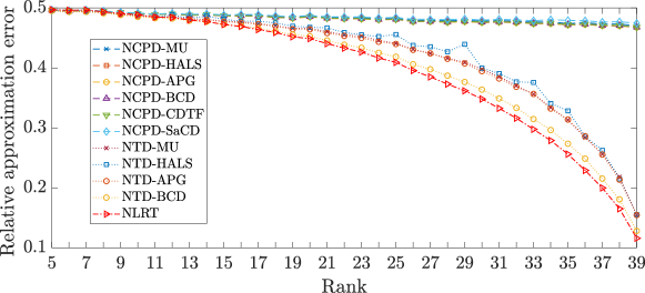
(a) Tensor size: $40\times 40\times 40$

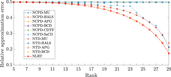
(b) Tensor size: $30\times 30\times 30\times 30$

Figure 1: Relative approximation errors on the randomly generated tensors in Case 2 with respect to the different rank settings.

The relative approximation errors in Case 2 with respect to different values of $r$ are plotted in Fig. 1. As we stated, the tensor of a given size will be fixed once generated. Then, for different values of $r$, we run each algorithm 10 times and the averaged values are plotted. From Fig. 1, we can see that the proposed NLRT method and NTD-BCD perform better than the other methods. For the tensors of the size $40\times 40\times 40$, the superior of our method over NTD-BCD is obvious when the rank is in between 27 and 39.

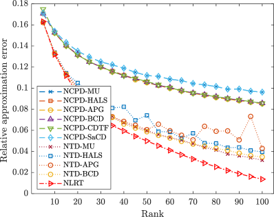
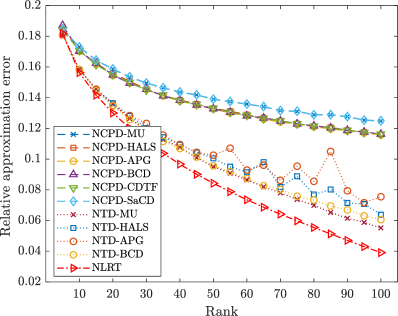
(a) “foreman”		(b) “coastguard”
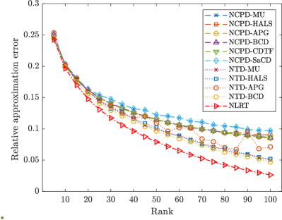
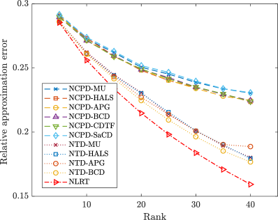
(c) “news”		(d) “basketball”

Figure 2: Relative approximation errors on 4 videos (100 frames) with respect to the different rank settings.

4.3 Video Data

In this subsection, we select 5 videos to test our method on the task of approximation. Three videos (respectively named “foreman”, “coastguard”, and “news”) are of the size $144\times 176\times 100$ (height$\times$width$\times$frame) and one (named “basketball”) is of the size $44\times 256\times 40$. One long video (named “bridge-far”) of the size $144\times 176\times 2000$ is also selected to test the approximation ability for large scale data. Firstly, we set the multilinear rank to be $(r,r,\cdots,r)$ and the CP rank to be $r$. We test our method to approximate these five videos with varying $r$ from 5 to 100. Moeover, we add the Gaussian noise to the video “coastguard” with different noise levels ($\text{SNR}_{\text{dB}}$ = 20, 30 ,40, 50), and test the approximation ability of differen methods for the noisy video data.

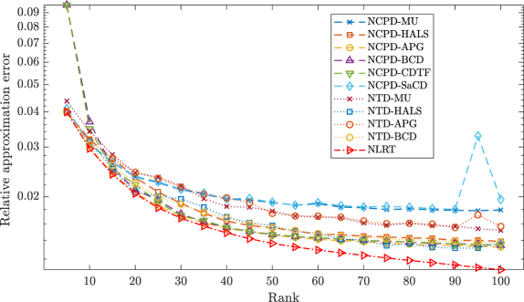
Figure 3: Relative approximation errors on the video “bridge-far” (2000 frames) with respect to the different rank settings.

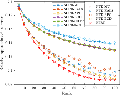
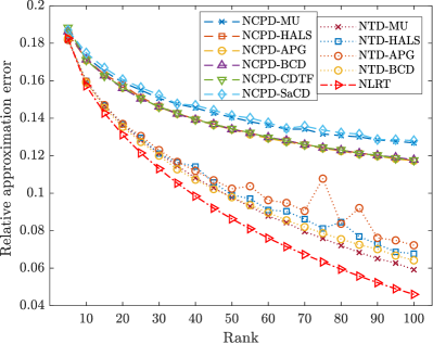
(a) SNR = 20 dB	(b) SNR = 30 dB
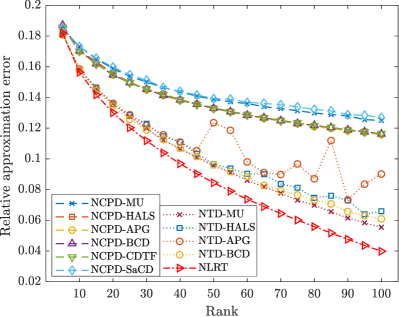
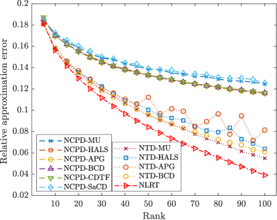
(c) SNR = 40 dB	(d) SNR = 50 dB

Figure 4: Relative approximation errors on the noisy video “coastguard” with respect to different rank settings and different noise levels.

We plot the relative approximation errors with respect to $r$ on 5 videos in Figs. 2 and 3. Although, for some videos the approximation errors of the results by NCPD methods are much higher than others, owing to that setting CP rank as $r$ largely constrained the model representation ability, we can still see that the potential of NCPD methods are promising. For example, for the videos “news” and “bridge-far”, NCPD methods are even occasionally superior to NTD methods. Thus, the comparison with NCPD methods provides some insights. From Figs. 2 and 3, it can be seen that the approximation errors of the results by our method are the lowest. Fig. 4 shows the relative approximation errors on the noisy video “coastguard” with respect to $r$. Similarly, our method achieves the lowest approximation errors on the video “coastguard” with respect to different rank settings and different noise levels. In Table 4, we list the average running time of each method.

Table 4: The average running time (in seconds) of different methods on video data.

Video	$\#$	NCPD-							NTD-					NLRT
	frames	MU	HALS	APG	BCD	CDTF	SaCD		MU	HALS	APG	BCD
“foreman”	100	60	66	55	24	23	45		202	188	354	74		20
“news”	100	46	46	37	17	16	33		176	197	313	59		25
“coastguard”	100	35	36	30	13	12	27		129	165	228	46		15
“basketball”	40	16	17	11	3	3	12		25	20	34	14		15
“bridge-far”	2000	386	173	265	186	188	209		183	211	299	511		296
Video	SNR	NCPD-							NTD-					NLRT
	(dB)	MU	HALS	APG	BCD	CDTF	SaCD		MU	HALS	APG	BCD
“coastguard”	20	28	29	28	9	9	20		135	146	258	46		18
	30	28	29	29	10	10	20		133	145	254	46		17
	40	28	29	29	10	10	20		134	147	255	47		16
	50	28	29	29	10	9	20		136	143	259	46		15

4.4 Hyperspectral Data

In this subsection, we test different methods on the hyperspectral data. We consider four hyperspectral images (HSIs): a subimage of Pavia City Center dataset of the size $200\times 200\times 80$ (height$\times$width$\times$spectrum), a subimage of Washington DC Mall dataset of the size $200\times 200\times 160$, the RemoteImage of the size $200\times 200\times 89$, and a subimage of Curprite dataset of the size $150\times 150\times 150$. Meanwhile, a hyperspectral video (HSV) of the size $120\times 188\times 33\times 31$ (height$\times$width$\times$spectrum$\times$time) is also selected to test the effectiveness of different methods on the fourth order tensor.

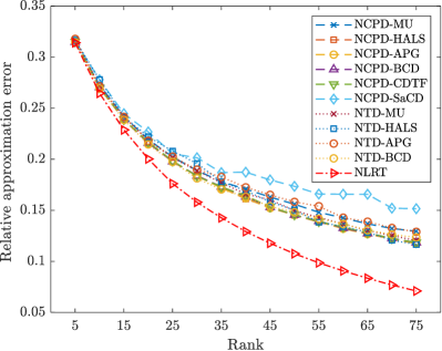
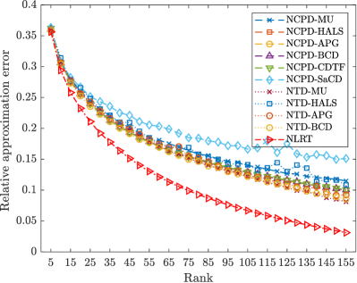
(a) Pavia City Center	(b) Washington DC Mall
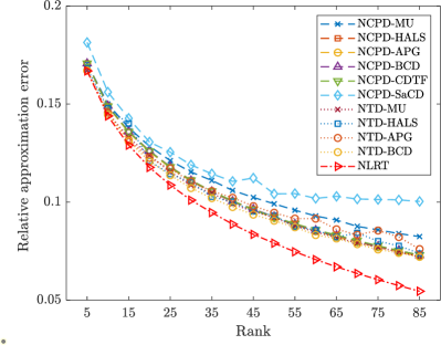
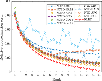
(c) RemoteImage	(d) Curprite

Figure 5: Relative approximation errors on 4 HSIs with respect to the different rank settings.

Figs. 5 and 6 report the relative approximation errors with respect to different values of rank $r$, i.e., multilinear rank = ($r,r,r$) or ($r,r,r,r$) and CP rank = $r$. It is evidently that the relative approximation errors by our NLRT are the lowest among all the methods. It is interesting to note that the difference between our method and NTD-BCD (the second best comparison method) is more significant than that on the synthetic fourth order tensor data.

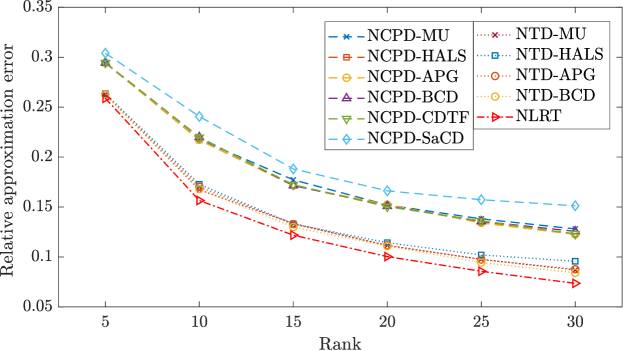
Figure 6: Relative approximation errors on the HSV with respect to the different rank settings.

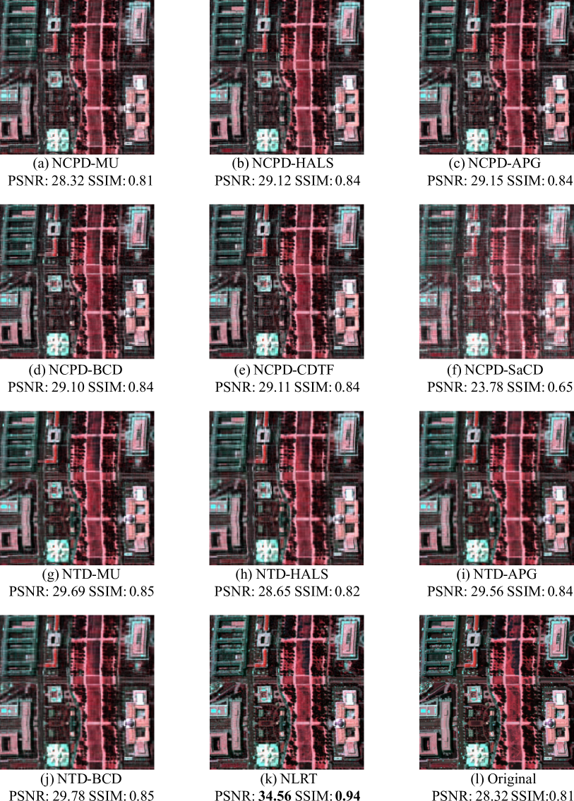
Figure 7: The pseudo-color images composed of the 113-th, 2-nd, and 16-th bands of the non-negative low-rank approximations by different methods when setting the rank $100$ on the Washington DC Mall.

In Fig. 7, we display the pseudo-color images of the results on the Washington DC Mall dataset with the multilinear rank (100,100,100) and CP rank = 100. The pseudo-color image is composed of the 113-th, 2-nd, and 16-th bands as the red, green, and blue channels, respectively. We also compute two image quality assessments (IQAs): the peak signal to noise ratio (PSNR) and the structural similarity index (SSIM) wang2004image of all the spectral bands for each band. Higher values of these two indexes indicate better reconstruction quality. In Fig. 7, we report the mean values across spectral bands of these two IQAs. It can be found in Fig. 7 that both visual and quality assessments of the NCPD methods are comparable to NTD methods. The proposed NLRT method largely outperforms other methods in terms of two IQAs, achieving the first place.

4.5 Selection of Features

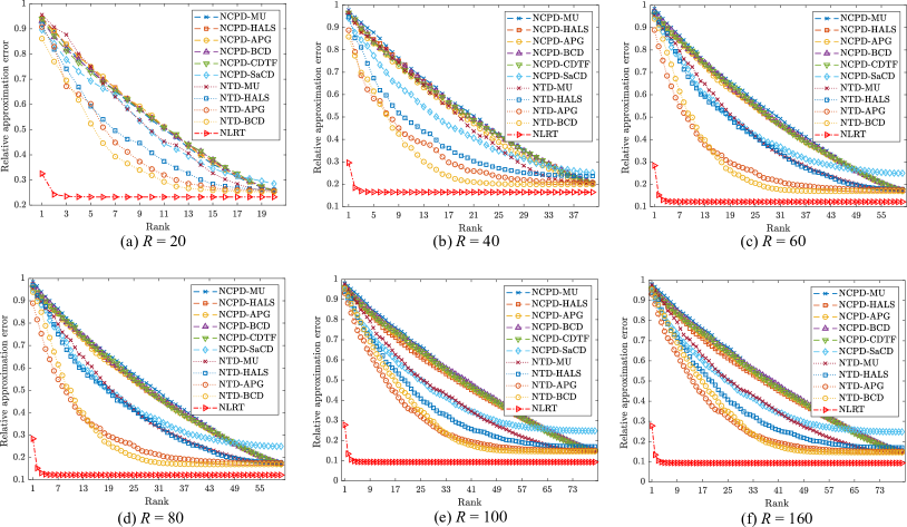
Figure 8: The comparison of relative residuals with respect to the number of mode-3 components to be used in the tensor approximation with $R=20,40,60,80,160$ for the hyperspectral image Washington DC Mall.

One advantage of the proposed NLRT method is that it can provide a significant index based on singular values of unfolding matrices song2020nonnegative that can be used to identify important singular basis vectors in the approximation. Those singular values and singular vectors are natural concomitants brought out by our algorithm without additional computations of SVD.

Here we take the HSI Washington DC Mall as an example. We compute the low-rank approximations of the proposed NLRT method and the other comparison methods with multlinear rank $(r,r,r)$ and CP rank $r$ for $r=20,40,60,80,160$. For the approximation results by NCPD methods,

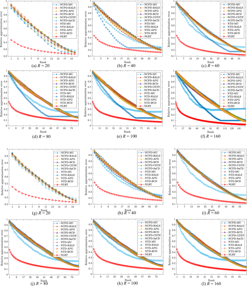
Figure 9: The comparison of relative residuals with respect to the number of the first mode (upper two rows from (a) to (f)) and the second mode (bottom two rows from (g) to (l)) components to be used in the tensor approximation with $R=20,40,60,80,160$ for the hyperspectral image Washington DC Mall.

we normalize the base vectors in 22 such that the $\ell_{2}$ norms of $\mathbf{a}^{k,1}$, $\mathbf{a}^{k,2}$ and $\mathbf{a}^{k,3}$ are equal to 1, and rearrange the resulting values $\lambda^{\prime}_{z}$ in the descending order in the CP decomposition. In Fig. 8, we plot

$$\|\mathcal{A}-\mathcal{X}_{\text{NCPD}}(j)\|_{F}/\|\mathcal{A}\|_{F}$$

with respect to $j$, where $\mathcal{X}_{\text{NCPD}}(j)=\sum^{j}_{k=1}\lambda^{\prime}_{k}\mathbf{a}^{k,1}\otimes\mathbf{a}^{k,2}\otimes\mathbf{a}^{k,3}$. Similarly, for the results of NTD methods, we also plot

$$\|\mathcal{A}-\mathcal{X}_{\text{NTD}}(j)\|_{F}/\|\mathcal{A}\|_{F}$$

with respect to $j$, where $\mathcal{X}_{\text{NTD}}(j)=[\mathcal{G}\times_{1}\mathbf{U}^{(1)}\times_{2}\mathbf{U}^{(2)}]_{:,:,\mathbf{k}_{j}}\times_{3}\mathbf{U}^{(3)}_{:,\mathbf{k}_{j}}$, $[\mathcal{G}\times_{1}\mathbf{U}^{(1)}\times_{2}\mathbf{U}^{(2)}]_{:,:,\mathbf{k}_{j}}$ is the $\mathbf{k}_{j}$-th mode-12 (spatial) slice of $[\mathcal{G}\times_{1}\mathbf{U}^{(1)}\times_{2}\mathbf{U}^{(2)}]$, and each $[\mathcal{G}\times_{1}\mathbf{U}^{(1)}\times_{2}\mathbf{U}^{(2)}]_{:,:,\mathbf{k}_{j}}$ is normalized with its Frobenius norm equaling to 1, and $\mathbf{k}_{j}$ indicates a vector composed of the indexes corresponding to the $j$ largest $\ell_{2}$ norms of $\mathbf{U}^{(3)}$’s columns. For the results by our methods, we plot

$$\|\mathcal{A}-\mathcal{X}_{\text{NLRT}}(j)\|_{F}/\|\mathcal{A}\|_{F}$$

with respect to $j$, where $\mathcal{X}_{\text{NLRT}}(j)=\textrm{fold}\left(\sum_{i=1}^{j}\sigma_{i}(\mathbf{X}_{3}){\bf u}_{i}(\mathbf{X}_{3}){\bf v}_{i}^{T}(\mathbf{X}_{3})\right)$, $\sigma_{i}(\mathbf{X}_{3})$ is the $i$-th singular values of ${\bf X}_{3}$, and ${\mathbf{X}}_{3}$ is the third-mode unfolding matrix of $\mathcal{X}$. The third-mode of ${\cal X}$ is chosen in NTD and our NLRT, we are interested to observe how many indices required in the spectral mode of given hyperspectral data.

In Fig. 8, we can see that when the number of components (namely $j$) increases, the relative residual decreases. Our NLRT could provide a significant index based on singular values to identify important singular basis vectors for the approximation. Thus, the relative residuals by the proposed NLRT algorithm are significantly smaller than those by the testing NTD and NCPD algorithms. Similar phenomena can be found in Fig. 9, in which $\mathcal{X}_{\text{NTD}}(j)$ and $\mathcal{X}_{\text{MP-NLRT}}(j)$ are computed using the number of indices in the first or second modes of ${\cal X}$.

4.6 Image Classification

The advantage of the proposed NLRT method is that the important singular basis vectors can be identified within the algorithm. Such basis vectors can provide useful information for image recognition such as classification. Here we conduct hyperspectral image classification experiments on the Indian Pines dataset. This data set was captured by the Airborne Visible/Infrared Imaging Spectrometer (AVIRIS) sensor over the Indian Pines test site in North-western Indiana in June 1992. After removing 20 bands, which cover the region of water absorption, this HSI is of the size $145\times 145\times 200$. The ground truth contains 16 land cover classes as shown in Fig. 10. Therefore, we set the multilinear rank to be $(16,16,16)$ and the CP rank to be 16 for all the testing methods. We randomly choose $s$ of the available labeled samples, which are exhibited in Table 5. Labeled samples from each class are used for training and the remaining samples are used for testing.

Table 5: The number of label samples in each class.

No.	1	2	3	4	5	6	7	8
Name	Alfalfa	Corn-	Corn-	Corn	Grass-	Grass-	Grass-pasture-	Hay-
		no till	min till		pasture	trees	mowed	windrowed
Samples	46	1428	830	237	483	730	28	478
No.	9	10	11	12	13	14	15	16
Name	Oat	Soybean-	Soybean-	Soybean-	Wheat	Woods	Buildings-Grass-	Stone-
		no till	min till	clean			Trees-Drives	Steel-Towers
Samples	20	972	2455	593	205	1265	386	93

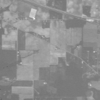
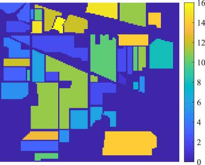
(a) The 10-th band of the original HSI.	(b) The ground truth categorization map.

Figure 10: Indian Pines image and related ground truth categorization information.

After obtaining low rank approximations, 16 singular vectors corresponding to the largest 16 singular values of the unfolding matrix of the tensor approximation along the spectral mode (the third mode) are employed for classification. We apply the $k$-nearest neighbor ($k$-NN, $k=1,3,5$) classifiers to identify the testing samples in the projected trained samples representation. The classification accuracy, which is defined as the portion of correctly identified entries, with respect to different $s$ is reported in Table 6. The results in Table 6 show that the classification based on our nonnegative low rank approximation is better than other comparison methods.

Table 6: The accuracy (in terms of percentage) of the classification results on the approximations by different methods. The best values are highlighted in bold.

$s$	Classi-		NCPD-							NTD-					NLRT
	fier		MU	HALS	APG	BCD	CDTF	SaCD		MU	HALS	APG	BCD
10	1-NN		69.68	69.71	67.91	66.40	65.56	61.50		65.89	71.12	73.98	73.70		74.92
	3-NN		63.79	64.72	61.89	61.52	60.57	58.00		61.65	65.25	69.80	68.02		70.12
	5-NN		62.11	62.72	60.46	60.23	59.21	56.58		61.26	63.67	67.53	65.68		68.38
20	1-NN		77.04	77.35	75.05	74.78	74.74	67.95		73.14	79.21	81.16	81.51		82.06
	3-NN		72.09	72.39	70.59	69.80	69.53	63.76		69.15	75.20	77.45	76.69		77.47
	5-NN		69.59	70.10	68.31	68.54	67.60	63.43		67.53	73.16	75.12	74.55		75.60
30	1-NN		81.20	81.01	78.82	79.28	78.36	71.36		76.76	83.19	84.24	85.03		85.71
	3-NN		76.76	76.84	74.44	74.37	73.95	68.13		72.11	78.68	80.12	80.91		81.62
	5-NN		74.06	74.52	72.38	72.21	72.14	66.46		71.18	76.54	78.29	78.74		79.16
40	1-NN		84.19	84.32	81.78	82.09	82.01	74.79		79.38	86.36	86.80	87.18		88.51
	3-NN		80.17	79.96	77.99	77.99	78.14	71.17		75.49	81.76	83.93	84.11		84.87
	5-NN		78.09	78.34	76.14	75.82	75.87	69.84		74.40	79.80	81.73	81.94		82.98
50	1-NN		85.73	86.27	83.50	83.89	83.81	77.15		82.14	88.09	88.16	88.81		90.19
	3-NN		82.31	82.14	79.91	80.23	80.42	73.95		78.10	83.95	85.98	85.96		86.52
	5-NN		80.19	80.60	77.94	78.32	78.12	72.21		76.95	81.92	84.05	84.03		84.79

5 Conclusion

In the paper, we proposed a new idea for computing nonnegative low rank tensor approximation. We proposed a method called NLRT which determines a nonnegative low rank approximation to given data by taking use of low rank matrix manifolds and non-negativity property. The convergence analysis is given. Experiments in synthetic data sets and multi-dimensional image data sets are conducted to present the performance of the proposed NLRT method. It shows that NLRT is better than classical nonnegative tensor factorization methods.

- (1) Attouch, H., Bolte, J., Redont, P., Soubeyran, A.: Proximal alternating minimization and projection methods for nonconvex problems: An approach based on the kurdyka-łojasiewicz inequality. Mathematics of Operations Research 35(2), 438–457 (2010)
- (2) Balasubramaniam, T., Nayak, R., Yuen, C.: Efficient nonnegative tensor factorization via saturating coordinate descent. ACM Transactions on Knowledge Discovery from Data (TKDD) 14(4), 1–28 (2020)
- (3) Bauschke, H.H., Luke, D.R., Phan, H.M., Wang, X.: Restricted normal cones and the method of alternating projections: applications. Set-Valued and Variational Analysis 21(3), 475–501 (2013)
- (4) Bauschke, H.H., Luke, D.R., Phan, H.M., Wang, X.: Restricted normal cones and the method of alternating projections: theory. Set-Valued and Variational Analysis 21(3), 431–473 (2013)
- (5) Cichocki, A., Phan, A.H.: Fast local algorithms for large scale nonnegative matrix and tensor factorizations. IEICE Transactions on Fundamentals of Electronics, Communications and Computer Sciences 92(3), 708–721 (2009)
- (6) Cichocki, A., Zdunek, R., Amari, S.i.: Hierarchical ALS algorithms for nonnegative matrix and 3D tensor factorization. In: International Conference on Independent Component Analysis and Signal Separation, pp. 169–176. Springer (2007)
- (7) Clarke, F., Vinter, R.: Regularity properties of optimal controls. SIAM Journal on Control and Optimization 28(4), 980–997 (1990)
- (8) De Lathauwer, L., De Moor, B., Vandewalle, J.: A multilinear singular value decomposition. SIAM Journal on Matrix Analysis and Applications 21(4), 1253–1278 (2000)
- (9) De Lathauwer, L., De Moor, B., Vandewalle, J.: On the best rank-1 and rank-(r 1, r 2,…, rn) approximation of higher-order tensors. SIAM journal on Matrix Analysis and Applications 21(4), 1324–1342 (2000)
- (10) Drusvyatskiy, D., Ioffe, A., Lewis, A.: Alternating projections and coupling slope. arXiv preprint arXiv:1401.7569 pp. 1–17 (2014)
- (11) Golub, G.H., Van Loan, C.F.: Matrix computations, vol. 3. JHU Press (2012)
- (12) Kim, Y.D., Choi, S.: Nonnegative Tucker decomposition. In: 2007 IEEE Conference on Computer Vision and Pattern Recognition, pp. 1–8. IEEE (2007)
- (13) Kolda, T.G., Bader, B.W.: Tensor decompositions and applications. SIAM Review 51(3), 455–500 (2009)
- (14) Kroonenberg, P.M.: Applied multiway data analysis, vol. 702. John Wiley & Sons (2008)
- (15) Lewis, A.S., Luke, D.R., Malick, J.: Local linear convergence for alternating and averaged nonconvex projections. Foundations of Computational Mathematics 9(4), 485–513 (2009)
- (16) Lewis, A.S., Luke, D.R., Malick, J.: Local linear convergence for alternating and averaged nonconvex projections. Foundations of Computational Mathematics 9(4), 485–513 (2009)
- (17) Lewis, A.S., Malick, J.: Alternating projections on manifolds. Mathematics of Operations Research 33(1), 216–234 (2008)
- (18) Li, G., Pong, T.K.: Douglas–rachford splitting for nonconvex optimization with application to nonconvex feasibility problems. Mathematical Programming 159(1-2), 371–401 (2016)
- (19) Li, X., Ng, M.K., Cong, G., Ye, Y., Wu, Q.: MR-NTD: Manifold regularization nonnegative Tucker decomposition for tensor data dimension reduction and representation. IEEE Transactions on Neural Networks and Learning Systems 28(8), 1787–1800 (2016)
- (20) Noll, D., Rondepierre, A.: On local convergence of the method of alternating projections. Foundations of Computational Mathematics 16(2), 425–455 (2016)
- (21) Pan, J., Ng, M.K., Liu, Y., Zhang, X., Yan, H.: Orthogonal nonnegative tucker decomposition. arXiv preprint arXiv:1912.06836 (2019)
- (22) Rockafellar, R.T., Wets, R.J.B.: Variational analysis, vol. 317. Springer Science & Business Media (2009)
- (23) Shin, K., Sael, L., Kang, U.: Fully scalable methods for distributed tensor factorization. IEEE Transactions on Knowledge and Data Engineering 29(1), 100–113 (2016)
- (24) Sidiropoulos, N.D., De Lathauwer, L., Fu, X., Huang, K., Papalexakis, E.E., Faloutsos, C.: Tensor decomposition for signal processing and machine learning. IEEE Transactions on Signal Processing 65(13), 3551–3582 (2017)
- (25) Song, G.J., Ng, M.K.: Nonnegative low rank matrix approximation for nonnegative matrices. Applied Mathematics Letters p. 106300 (2020)
- (26) Tucker, L.R.: Some mathematical notes on three-mode factor analysis. Psychometrika 31(3), 279–311 (1966)
- (27) Wang, Z., Bovik, A.C., Sheikh, H.R., Simoncelli, E.P.: Image quality assessment: from error visibility to structural similarity. IEEE Transactions on Image Processing 13(4), 600–612 (2004)
- (28) Welling, M., Weber, M.: Positive tensor factorization. Pattern Recognition Letters 22(12), 1255–1261 (2001)
- (29) Xu, Y., Hao, R., Yin, W., Su, Z.: Parallel matrix factorization for low-rank tensor completion. Inverse Problems and Imaging 9(2), 601–624 (2015)
- (30) Xu, Y., Yin, W.: A block coordinate descent method for regularized multiconvex optimization with applications to nonnegative tensor factorization and completion. SIAM Journal on Imaging Sciences 6(3), 1758–1789 (2013)
- (31) Zhang, Y., Zhou, G., Zhao, Q., Cichocki, A., Wang, X.: Fast nonnegative tensor factorization based on accelerated proximal gradient and low-rank approximation. Neurocomputing 198, 148–154 (2016)
- (32) Zhou, G., Cichocki, A., Xie, S.: Fast nonnegative matrix/tensor factorization based on low-rank approximation. IEEE Transactions on Signal Processing 60(6), 2928–2940 (2012)