merlin: An R package for Mixed Effects Regression for Linear, Nonlinear and User-defined models

Emma C. Martin, Alessandro Gasparini, Michael J. Crowther merlin: An R package for Mixed Effects Regression for Linear, Nonlinear and User-defined models merlin: Mixed Effects Regression The R package merlin performs flexible joint modelling of hierarchical multi-outcome data. Increasingly, multiple longitudinal biomarker measurements, possibly censored time-to-event outcomes and baseline characteristics are available. However, there is limited software that allows all of this information to be incorporated into one model. In this paper, we present merlin which allows for the estimation of models with unlimited numbers of continuous, binary, count and time-to-event outcomes, with unlimited levels of nested random effects. A wide variety of link functions, including the expected value, the gradient and shared random effects, are available in order to link the different outcomes in a biologically plausible way. The accompanying predict.merlin function allows for individual and population level predictions to be made from even the most complex models. There is the option to specify user-defined families, making merlin ideal for methodological research. The flexibility of merlin is illustrated using an example in patients followed up after heart valve replacement, beginning with a linear model, and finishing with a joint multiple longitudinal and competing risks survival model. joint modelling, multi-outcome, mixed effects, survival, R, merlin joint modelling, multi-outcome, R, merlin Emma C. Martin
University of Leicester
Department of Health Sciences, University Road, Leicester, LE1 7RH, UK
E-mail:
Alessandro Gasparini
Karolinska Institutet
Department of Medical Epidemiology and Biostatistics, Stockholm, Sweden
E-mail:
Michael J. Crowther
University of Leicester &
Karolinska Institutet
Department of Health Sciences, University Road, Leicester, LE1 7RH, UK & Department of Medical Epidemiology and Biostatistics, Stockholm, Sweden
E-mail:

1 Introduction

Software packages to fit joint and multi-state models are continuously being developed and updated to increase flexibility. However this flexibility is often limited in terms of outcome types, levels of nested random-effects, or the forms of linking functions between outcomes. We have developed merlin in order to address this lack of flexibility, allowing for a wide range of models to be estimated. With merlin it is possible to include any number of outcomes from a wide range of families, including Gaussian, Bernoulli, Poisson, a number of survival models including flexible parametric models, amongst others. It is also possible to custom supply user defined families to allow for even greater flexibility and method development. This allows merlin to fit everything from a simple Weibull model to a multivariate joint model. Joint models can be defined using commonly chosen association structures (Gould2015a), for example, shared random effects, the current value, gradient or area under the curve, and to provide even more customisation - user defined link functions. This R package is based on the recently released merlin package in Stata (Crowther2017, merlinStata).

Previous software released in R has some of the individual capabilities of merlin. Package JM (JM) fits a single normal longitudinal response jointly with a single survival outcome or competing risk outcomes, assuming a current value or current gradient link. There is also an extension JMbayes (JMbayes) which fits similar models in a Bayesian framework. joineR (joineR) allows for the joint modelling of a single longitudinal response and a single time-to-event outcome or competing risk outcome. The extension joineRML (joineRML) additionally allows for multivariate longitudinal data. The frailtypack (frailtypack) package fits shared, joint and nested frailty models, with one longitudinal response and multiple recurrent and terminal events.

New package merlin offers additional flexibility in how the joint model is specified. Multiple longitudinal responses can be specified and there is a wider range of models available to better describe the data, including splines and fractional polynomials. There is also a wider variety of survival models available compared to joineR which only allows Cox models, and JM and frailtypack which allow Cox, Weibull and limited spline based survival models. In addition to these models, merlin allows for exponential survival models, and a wider range of flexible spline based models such as Royston-Parmar models (Royston2001). While it is possible to fit models with multiple shared random-effects, there are additional link functions available to describe the relationship between the longitudinal and time-to-event outcomes, including current expected value, or other functions of the longitudinal response, including derivatives and integrals. A number of packages exist which allow for multiple hierarchical levels of random-effects for either longitudinal responses (lme4 (lme4) or nlme (nlme)) or time-to-event outcomes (coxme (coxme)). Each of the joint modelling packages described above only allow for one level of clustering, with the exception of frailtypack which allows for two, whereas merlin can incorporate any number of nested levels, which is particularly useful for big data such as electronic health records, which is often hierarchical.

Further flexibility is provided in merlin with the option of user-defined functions. This allows users to define their own likelihood functions, merlin is then used as a wrapper function to carry out the optimisation, similar to BAMLSS (BAMLSS) which uses a modular “Lego brick” approach in a Bayesian framework. Allowing users to extend merlin via user-defined functions makes it a useful tool for the development of new methods.

In this paper we introduce the modular syntax employed by merlin which enables its flexibility. In order to illustrate this flexibility we will develop an example model using data from an observational study of patients following aortic valve replacement surgery (Lim2008). In Section 2 we explain the syntax to specify the model structure and use the predict function. In Section 3 we work through an illustrative example in patients following heart valve replacement. Finally in Section 4 we discuss the advantages of using merlin and plans for future extensions.

2 Specifying model structure

2.1 Syntax

The syntax for merlin is modular in nature. The family is specified for each outcome, the linear predictor for each outcome can then be built from components such as an intercept, covariates and random effects.

merlin(model = list(model1, model2, ...),
       family = c("family1", "family2", ...),
       levels = "level1",
       data = data))

Where the syntax for each model is

model1 <- depvar   component1 + component2 + …, model_options

Each component can be made up of a number of elements such as covariates, random effects, functions of time and expected values of other outcomes. Interactions between elements can be specified using : between different elements. By default a coefficient will be estimated for each component, the coefficient can be constrained to 1 using *1.

component1 <- element1 [:element2] [:element3] […] [*1]

A number of model families are currently available, including

• gaussian - Gaussian distribution

• bernoulli - Bernoulli distribution

• poisson - Poisson distribution

• beta - beta distribution

• negbinomial - Negative binomial distribution

As well as a number of survival models

• exponential - exponential survival distribution

• weibull - Weibull distribution

• gompertz - Gompertz distribution

• rp - Royston-Parmar survival model, (complex predictor on the log cumulative hazard scale)

• loghazard - general log hazard model (complex predictor on the log hazard scale)

With two user-defined options

• user - which fits a user-defined model which can be written using merlin’s utility functions. The name of the user-defined function needs to be passed through using userf option

• null - which is a convenience tool for defining additional complex predictors, that do not contribute to the log likelihood

2.2 Element types

Each element can take a number of different forms

• varname - the simplest form is a varname, which refers to a variable in the data set provided.

• rcs - a restricted cubic spline function,

  • knots() - allows the user to specify the location of the knots in the form of a vector.

  • df() - alternatively the number of degrees of freedom can be specified, in which case the boundary knots are assumed to be at the minimum and maximum of varname with the internal knots placed at evenly spaced centiles.

  • orthog - this option uses Gram-Schmidt orthogonalisation of the splines, specifying this can improve model convergence.

• time functions - such as powers of time and log time. In order to use time functions timevar must be specified as extra numerical integration may be required.

• M#[cluster level] - a random-effect at the cluster level, all random-effects must be named M followed by a number to enable the sharing of random effects between models

• fp() - specifies a fractional polynomial function, with order 1 or 2.

  • powers() - the powers of the the fractional polynomial function must be specified (up to second degree).

• bhazard(varname) - invokes a relative survival (excess hazard) model. varname specifies the expected hazard rate at the event time.

• exposure(varname) - include log(varname) in the linear predictor, with a coefficient of 1. For use with family = "poisson".

Functions of longitudinal submodels can be included as covariates in other submodels using the following options

• EV[depvar] - the expected value of the response of a submodel

• dEV[depvar] - the first derivative with respect to time of the expected value of the response of a submodel

• d2EV[depvar] - the second derivative with respect to time of the expected value of the response of a submodel

• iEV[depvar] - the integral with respect to time of the expected value of the response of a submodel

• XB[depvar] - the expected value of the complex predictor of a submodel

• dXB[depvar] - the first derivative with respect to time of the expected value of the complex predictor of a submodel

• d2XB[depvar] - the second derivative with respect to time of the expected value of the complex predictor of a submodel

• iXB[depvar] - the integral with respect to time of the expected value of the complex predictor of a submodel

2.3 Integration methods

There are a number of methods available for numerically integrating out the random-effects in order to calculate the likelihood for a mixed-effects model. The options for intmethod are:

• ghermite - for non-adaptive Gauss-Hermite quadrature;

• halton - for Monte Carlo integration using Halton sequences;

• sobol - for Monte Carlo integration using Sobol sequences;

• mc - for standard Monte Carlo integration using normal draws.

The default is ghermite. Level-specific integration techniques can be specified. Gauss-Hermite quadrature is widely considered the optimal numerical integration technique, however it doesn’t scale well for large numbers of random-effects. Therefore in a three level model example, we may use Gauss-Hermite quadrature at the highest level and the more efficient Monte-Carlo integration with Halton sequences at level 2, using intmethod = c("ghermite", "halton").

2.4 Post estimation

A range of post estimation tools are available with merlin using the prediction function using the following syntax.

predict(modelname, statistic, type, options)

The currently available statistics options are

• eta - the expected value of the complex predictor

• mu - the expected value of the response variable

• hazard - the hazard function

• chazard - the cumulative hazard function

• logchazard - the log cumulative hazard function

• survival - the survival function

• cif - the cumulative incidence function

• rmst - calculates the restricted mean survival time, which is the integral of the survival function within the interval (0,t], where t is the time at which predictions are made. If multiple survival models have been specified in your merlin model, then it will assume all of them are cause-specific competing risks models, and include them in the calculation. If this is not the case, you can override which models are included by using the causes option. rmst = t - totaltimelost.

• cifdifference calculates the difference in cif predictions between values of a covariate specified using the contrast option.

• hdifference calculates the difference in hazard predictions between values of a covariate specified using the contrast option.

• rmstdifference calculates the difference in rmst predictions between values of a covariate specified using the contrast option.

• mudifference calculates the difference in mu predictions between values of a covariate specified using the contrast option.

• etadifference calculates the difference in eta predictions between values of a covariate specified using the contrast option.

• timelost - calculates the time lost due to a particular event occurring, within the interval (0,t]. In a single event survival model, this is the integral of the cif between (0,t]. If multiple survival models are specified in the merlin model then by default all are assumed to be cause-specific event time models contributing to the calculation. This can be overridden using the causes option.

• totaltimelost - total time lost due to all competing events, within (0,t]. If multiple survival models are specified in the merlin model then by default all are assumed to be cause-specific event time models contributing to the calculation. This can be overridden using the causes option. totaltimelost is the sum of the timelost due to all causes.

Prediction options include

• type - specifies whether the predictions include fixed-effects only (fixedonly), or the marginal prediction is calculated marginally with respect to the latent variables. The stat is calculated by integrating the prediction function with respect to all the latent variables over their entire support.

• predmodel - specifies which model to predict from, default predmodel=1.

• causes - for use when calculating predictions from a competing risks model. By default, cif, rmst, timelost and totaltimelost assume that all survival models included in the merlin model are cause-specific hazard models contributing to the calculation. If this is not the case, then you can specify which models (indexed using the order they appear in your merlin model by using the causes option, e.g. causes=c(1, 2)).

• at - specifies covariate values for prediction. Fixed values of covariates should be specified in a list e.g. at = c("trt" = 1, "age" = 50).

• contrast - specifies the values of a covariate to be used when comparing statistics, such as when using the cifdifference option to compare cumulative incidence functions, e.g. contrast = c("trt" = 0, "trt" = 1).

3 Examples

A consequence of the flexibility of merlin is the syntax is arguably complex to allow for the generalisation. In order to illustrate the potential uses of merlin we fit a number of increasingly advanced models to data from an observational study which investigated the effects of aortic valve replacement with a stentless or a homograft valve (Lim2008). The study followed 300 patients who underwent aortic valve replacement between 1991 and 2001, all patients with at least one year of follow-up were included. A number of baseline measurements were available such as age, sex, preoperative body surface area and size of valve. The dataset also includes longitudinal measures of valve gradient, standardised left ventricular mass index and ejection fraction from an average of four follow-up appointments per patient. We will use the copy of the data set available from R package joineRML (joineRML) to illustrate.

R> data(heart.valve, package = "joineRML")

As we are interested in fitting joint survival and longitudinal models, there must be at least one longitudinal biomarker measurement for each individual. We will primarily focus on valve gradient as our longitudinal outcome, therefore it is necessary to exclude any individual who doesn’t have at least one valve gradient observation.

R> heart.valve <- heart.valve[!is.na(heart.valve$grad),]\par Thedatashouldbesetoutinwideformatforsubmodel,witheachoutcomespecifiedinaseparatecolumn.Forsurvivaldataeventtimeandstatuswillappearindifferentcolumns,andshouldonlybespecifiedonceperindividual.Howeverwithinasubmodellongformatisused,witheachrepeatedmeasurementofabiomarkeronanewrowwithaseparatecolumnspecifyingthetimingofthatobservation.Thecurrentsetupofthe\code{heart.valve}data(shownbelow)needssomeeditingtoallowmodellingfittingwith\pkg{merlin},howeveroncethedatahasbeenputintothecorrectformat,allmodelscanbefittedwithoutanyfurthereditingbeingrequired.\par\CodeChunk\par\CodeInput R>print(R+heart.valve[heart.valve$numR+c(1:3,25,5:6,4,8,10)],R+row.names=FALSER+)\par\CodeOutput numsexagehsfuyrsstatustimelog.gradlog.lvmi1075.06027Stentlessvalve4.95616400.01095892.3025854.7789551075.06027Stentlessvalve4.95616403.67945202.3025854.7789551075.06027Stentlessvalve4.95616404.69589002.3025854.9245692045.79452Homograft9.66301406.36438402.6390574.7443232045.79452Homograft9.66301407.30411002.1972254.6986612045.79452Homograft9.66301408.30137002.4849075.05879013169.94247Homograft5.18630110.13698632.7080505.30554113169.94247Homograft5.18630111.05753402.8332135.28335613169.94247Homograft5.18630112.05479502.9957324.79455013169.94247Homograft5.18630113.97260303.4011974.993421\par Theeventtime(\code{fuyrs})foreachindividualshouldonlyappearonceinthedataset,unlesstherearemultipleeventsperindividual,theseshouldappearonseparatelines.The\code{status}istheeventindicatorvariable,coded0forcensored(losttofollow-up)and1fordied.\par\CodeChunk\par\CodeInput R>heart.valve$id<-heart.valve$numR>heart.valve$stime<-heart.valve$fuyrsR>heart.valve$stime[duplicated(heart.valve$id)]<-NAR>heart.valve$died<-heart.valve$statusR>heart.valve$died[duplicated(heart.valve$id)]<-NA\par Binaryvariables,suchastypeofheartvalveused,needtobeconvertedtobenumeric.\par\CodeChunk\par\CodeInput R>heart.valve$type<-as.numeric(heart.valve$hs)-1\par Asectionofthecorrectlyformatteddataisshownbelow,Individual1hasthreelongitudinalmeasurementsforlogvalvegradient(\code{log.grad})andlogleftventricularmassindex(\code{log.lvmi}),thetimingsofthesemeasurementsaregiveninthe\code{time}column.Inthiscasethedifferentbiomarkersweremeasuredatthesametimepoints,butthisisnotnecessary,missingbiomarkermeasurementsshouldberecordedas\code{NA}.Thesurvivalinformationhasbeenrecordedonthefirstlineforeachindividual.Baselinecovariatessuchassexshouldbespecifiedoneverylineforthatindividual.Allthemodelsbelowarefittedtothisdataset.\par\CodeChunk\par\CodeInput R>print(R+heart.valve[heart.valve$idR+c(26,2:3,29,27:28,8,10,4)],R+row.names=FALSER+)\par\CodeOutput idsexagetypestimediedlog.gradlog.lvmitime1075.0602714.95616402.3025854.7789550.01095891075.060271NANA2.3025854.7789553.67945201075.060271NANA2.3025854.9245694.69589002045.7945209.66301402.6390574.7443236.36438402045.794520NANA2.1972254.6986617.30411002045.794520NANA2.4849075.0587908.301370013169.9424705.18630112.7080505.3055410.136986313169.942470NANA2.8332135.2833561.057534013169.942470NANA2.9957324.7945502.054795013169.942470NANA3.4011974.9934213.9726030\par$

To begin with we will fit a simple linear regression of log of the valve gradient (log.grad) against time, with age and sex as covariates.

R> library(merlin) R> m1 <- merlin( R+ model = log.grad   sex + age + time, R+ family = "gaussian", R+ data = heart.valve R+ ) R> summary(m1)

Mixed effects regression model Log likelihood = -651.4753

Estimate Std. Error z Pr(>|z|) [95sex 0.140489 0.059778 2.350 0.0188 0.023327 0.257651 age -0.002212 0.002297 -0.963 0.3356 -0.006714 0.002290 time -0.013541 0.011958 -1.132 0.2574 -0.036978 0.009895 _cons 2.771597 0.160581 17.260 0.0000 2.456863 3.086330 log_sd(resid.) -0.383205 0.028194 -13.592 0.0000 -0.438465 -0.327946

The constant term for log valve gradient is estimated to be 2.772 (95% CI 2.457, 3.086) and this is estimated to change by -0.014 (95% CI -0.037, 0.010) for every year after valve replacement. The residual error is reported in the results table as the log of the standard deviation, meaning the residual standard error in this model is 0.682. To assess model fit we can calculate the residuals using the predict function to get the fitted values.

R> heart.valve$m1res<-heart.valve$log.grad - predict(m1, stat = "mu") R> R> library(ggplot2) R> ggplot(heart.valve, aes(x = time, y = m1res)) + R+ geom_point() + R+ geom_hline(yintercept = 0, color = "blue") + R+ xlab("Time (years)") + R+ ylab("Residual") + R+ theme_classic()

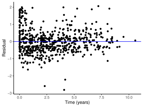
Figure 1: Absolute residuals plot against time for linear model m1

This shows that there seems to be some model misspecification, as the values at the beginning and end are generally under predicted, while values between 1 and 4 years are over predicted. To address this we can add further flexibility to the shape of the log valve gradient over time, using restricted cubic splines, with number degrees of freedom specified as below. The boundary knots will be assumed to be at the minimum and maximum of log.grad with the internal knots at equally spaced centiles. Alternatively the locations of the knots can be specified by using the knots() option. The spline terms have been orthogonalised, which will impact on the interpretation of the intercept term. While the spline terms themselves have little meaningful interpretation they are reported to allow the model to be used to make external predictions.

R> m2 <- merlin( R+ model = log.grad   sex + age + rcs(time, df = 3, orthog = TRUE), R+ timevar = "time", R+ family = "gaussian", R+ data = heart.valve R+ ) R> summary(m2)

Mixed effects regression model Log likelihood = -678.6148

Estimate Std. Error z Pr(>|z|) [95sex -0.090970 0.057917 -1.571 0.11625 -0.204486 0.022545 age 0.016740 0.002454 6.822 0.00000 0.011931 0.021550 rcs():1 -0.067805 0.026277 -2.580 0.00987 -0.119306 -0.016304 rcs():2 -0.215318 0.025901 -8.313 0.00000 -0.266084 -0.164553 rcs():3 0.097600 0.025675 3.801 0.00014 0.047278 0.147922 _cons 1.532048 0.159002 9.635 0.00000 1.220411 1.843685 log_sd(resid.) -0.448594 0.030335 -14.788 0.00000 -0.508050 -0.389139

When we plot the residuals for model m2 we can see there is less of a pattern over time, suggesting this model is a better fit to the data.

R> heart.valve$m2res<-heart.valve$log.grad - predict(m2, stat = "mu") R> ggplot(heart.valve, aes(x = time, y = m2res)) + R+ geom_point() + R+ geom_hline(yintercept = 0, color = "blue") + R+ xlab("Time (years)") + R+ ylab("Residual") + R+ theme_classic()

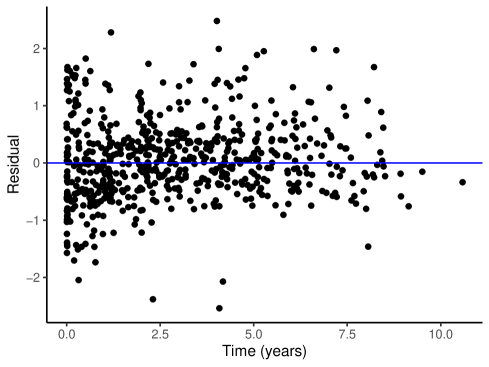
Figure 2: Absolute residuals plot against time for restricted cubic spline model m2

We can further improve this model by accounting for the clustered nature of the log.grad measurements within patients (id). We can add a normally-distributed random intercept at the patient id level using the M# syntax below. Each random effect is given a name of this form to enable the sharing of random effects between models, which will be illustrated later. In the model below M1 specifies a random intercept and M2 specifies a random linear slope. By default the random-effects at each level are not assumed to be correlated (option covariance(identity)), however this can be relaxed and the correlation estimated by instead specifying covariance(unstructured). For mixed-effects models the levels must be specified using the level option. There is no limit to the number of levels which can be fitted, but the levels must be be specified from highest to lowest, e.g. county > practice > patient. By default all components in the model will have an estimated coefficient, however the coefficient can be constrained to 1 using *1 notation, which would normally be the case for random effects not shared between models. By default estimation of the likelihood is done using Gauss-Hermite quadrature with 7 nodes, increasing this number using the ip option will improve estimation of the likelihood, although this will increase computation time considerably.

R> m3 <- merlin( R+ model = log.grad   sex + age + rcs(time, df = 3, orthog = TRUE) + R+ M1[id] * 1 + time:M2[id] * 1, R+ timevar = "time", R+ level = "id", R+ covariance = "unstructured", R+ family = "gaussian", R+ data = heart.valve R+ ) R> summary(m3)

Mixed effects regression model Log likelihood = -612.5806

Estimate Std. Error z Pr(>|z|) [95sex 0.1559667 0.0741357 2.104 0.0354 0.0106635 0.3012699 age 0.0057777 0.0030691 1.883 0.0598 -0.0002377 0.0117931 rcs():1 -0.0331820 0.0332446 -0.998 0.3182 -0.0983402 0.0319762 rcs():2 -0.1828734 0.0262125 -6.977 0.0000 -0.2342490 -0.1314978 rcs():3 0.1294719 0.0233294 5.550 0.0000 0.0837471 0.1751967 _cons 2.2338384 0.2030426 11.002 0.0000 1.8358823 2.6317945 log_sd(resid.) -0.7233108 0.0342331 -21.129 0.0000 -0.7904063 -0.6562152 log_sd(M1) -1.0672644 0.1262396 -8.454 0.0000 -1.3146895 -0.8198394 log_sd(M2) -0.7900452 0.1528337 -5.169 0.0000 -1.0895939 -0.4904966 atanh_corr(M2,M1) -2.1512169 0.1571694 -13.687 0.0000 -2.4592632 -1.8431706

Integration method: Non-adaptive Gauss-Hermite quadrature Integration points: 7

Adding the random-effects terms at the id level greatly reduces the log-likelihood. The standard deviation for the random intercept is 0.344, and for the random slope is 0.454. The correlation between these random-effects is reported as the inverse hyperbolic tangent, to get the estimate of the correlation the tanh() function can be used, tanh(-2.151) = -0.973 showing that these random-effects are highly correlated. Random-effects at multiple hierarchical levels can be included by changing the level variable in square brackets, and by specifying the levels from highest to lowest in the level option.

We can make predictions of the expected value of the response from mixed-effects model m3 using the predict function with the mu option. Predictions will only be made for non-missing values of the response. These predictions are marginal, calculated by integrating out the random-effects, giving population averaged predictions.

R> ldata <- heart.valve[!is.na(heart.valve$log.grad),]R>ldata$pred1 <- predict(m3, stat = "mu", predmodel = 1, type = "marginal") R> print( R+ ldata[ldata$idR+row.names=FALSER+)\par\CodeOutput idtimelog.gradpred110.01095892.3025853.12239113.67945202.3025852.52327814.69589002.3025852.64585426.36438402.6390572.60346827.30411002.1972252.64273328.30137002.4849072.665921130.13698632.7080503.177508131.05753402.8332132.720037132.05479502.9957322.514966133.97260303.4011972.689035\par$

As well as a wide range of standard models, merlin also allows users the flexibility to specify their own likelihood functions using the user family.

To help users to define their own likelihood there are a number of inbuilt utility functions.

• merlin_util_depvar(M) - returns the dependent variable for the current model. For time-to-event outcomes this will be a matrix with two columns, for event time and event-indicator.

• merlin_util_xzb(M, t) - returns the complex predictor for the current model, optionally evaluated at time t.

• merlin_util_xzb_deriv(M, t) - returns the derivative with respect to time of the complex linear predictor for the current model, optionally evaluated at time t.

• merlin_util_xzb_deriv2(M, t) - returns the second derivative with respect to time of the complex linear predictor for the current model, optionally evaluated at time t.

• merlin_util_xzb_integ(M, t) - returns the integral with respect to time of the complex linear predictor for model M, optionally evaluated at time t.

• merlin_util_expval(M, t) - returns the expected value of the response for the current model, optionally evaluated at time t.

• merlin_util_expval_deriv(M, t) - returns the derivative with respect to time of the expected value of the response for the current model, optionally evaluated at time t.

• merlin_util_expval_deriv2(M, t) - returns the second derivative with respect to time of the expected value of the response for the current model, optionally evaluated at time t.

• merlin_util_expval_integ(M, t) - returns the integral with respect to time of the expected value of the response for the current model,, optionally evaluated at time t.

• merlin_util_ap(M,i) - returns the ith ancillary parameter of the current model.

• merlin_util_timevar(M) - returns the time variable for he current model, specified by the timevar option.

These utility functions take a list as input, which has been referred to as gml below. This contains a merlin object, which should not then be edited by the user. The xzb or expval functions have a corresponding *_mod() function, which allows users to specify an additional argument for which model to call, e.g. merlin_util_xzb_mod(M,2) will return the complex predictor for the second model in the merlin statement, allowing submodels to be linked.

The log-likelihood is specified as a function, giving the observation level log-likelihood contribution. As an example a simple linear model can be fitted using the function below.

R> logl_gaussian <- function(gml) R+ y <- merlin_util_depvar(gml) R+ xzb <- merlin_util_xzb(gml) R+ se <- exp(merlin_util_ap(gml, 1)) R+ R+ mu <- (sweep(xzb, 1, y, "-"))^2 R+ logl <- ((-0.5 * log(2 * pi) - log(se)) - (mu / (2 * se^2))) R+ return(logl) R+

To specify a user defined function, the family is given as user, the userf option must then be given the function above.

R> m4 <- merlin(log.grad   sex + age + time + ap(1), R+ family = "user", R+ userf = "logl_gaussian", R+ data = heart.valve R+ ) R> summary(m4)

Mixed effects regression model Log likelihood = -651.4753

Estimate Std. Error z Pr(>|z|) [95sex 0.140489 0.059778 2.350 0.0188 0.023327 0.257651 age -0.002212 0.002297 -0.963 0.3356 -0.006714 0.002290 time -0.013541 0.011958 -1.132 0.2574 -0.036978 0.009895 _cons 2.771597 0.160581 17.260 0.0000 2.456863 3.086330 _ap1 -0.383205 0.028194 -13.592 0.0000 -0.438465 -0.327946

The parameter estimates from this model are the same as model M1 above, where _ap1 is the ancillary residual error parameter. These user defined functions allows users to extend merlin, which is particularly useful for those doing methodological research.

3.1 Survival / time-to-event analysis

A number of standard time-to-event models are available in merlin such as Weibull, exponential and Gompertz models. Additionally a range of more flexible models are also available including Royston-Parmar models, and a model on the log hazard scale, for both a number of forms can be used for the baseline including restricted cubic splines, or fractional polynomials.

3.1.1 Weibull proportional hazards model

We will start by fitting a simple Weibull proportional hazard model for time-to-death, adjusting for age and type of aortic valve replacement. In order to fit a survival model a Surv object must be supplied with the time and event indicator variables.

R> m5 <- merlin( R+ model = Surv(stime, died)   age + type, R+ family = "weibull", R+ data = heart.valve R+ ) R> summary(m5)