Abstract

The paper discusses what characteristic quantities could quantify nonequilibrium states of Bose systems. Among such quantities, the following are considered: effective temperature, Fresnel number, and Mach number. The suggested classification of nonequilibrium states is illustrated by studying a Bose-Einstein condensate in a shaken trap, where it is possible to distinguish eight different nonequilibrium states: weak nonequilibrium, vortex germs, vortex rings, vortex lines, deformed vortices, vortex turbulence, grain turbulence, and wave turbulence. Nonequilibrium states are created experimentally and modeled by solving the nonlinear Schrödinger equation.

1 Generation of nonequilibrium condensates

Weakly interacting atoms at asymptotically low temperature are almost completely Bose condensed, forming a coherent system. Such a system can be described in the quasiclassical approximation resulting in the equation for the coherent field corresponding to the nonlinear Schrödinger (NLS) equation

$$i\;\frac{\partial}{\partial t}\;\psi({\bf r},t)=\hat{H}[\;\psi\;]\;\psi({\bf r},t)\;,$$ (1)

in which the nonlinear Hamiltonian is

$$\hat{H}[\;\psi\;]=-\;\frac{\nabla^{2}}{2m}+U({\bf r},t)+N\int\Phi({\bf r}-{\bf r}^{\prime})\;|\;\psi({\bf r}^{\prime},t)\;|^{2}\;d{\bf r}^{\prime}\;.$$ (2)

Here the Planck constant is set to one, $U({\bf r},t)$ is an external potential, and $\Phi({\bf r})$ is the interaction potential of atoms. This equation was advanced by Bogolubov [1] in 1949 in his widely known book Lectures on Quantum Statistics (see also [2, 3, 4]).

For a dilute gas, the interaction potential is modeled by the local form

$$\Phi({\bf r})=\Phi_{0}\delta({\bf r})\qquad\left(\Phi_{0}\equiv 4\pi\;\frac{a_{s}}{m}\right)\;,$$ (3)

where $a_{s}$ is scattering length. Then the nonlinear Hamiltonian becomes

$$\hat{H}[\;\psi\;]=-\;\frac{\nabla^{2}}{2m}+U({\bf r},t)+N\Phi_{0}|\;\psi({\bf r},t)\;|^{2}\;.$$ (4)

The solution to the NLS equation is also called the condensate wave function. In the present case, it is normalized to one,

$$\int|\;\psi({\bf r},t)\;|^{2}\;d{\bf r}=1\;.$$ (5)

The stationary solution to the NLS equation corresponds to the situation where the external potential does not depend on time, or simply is absent, and the initial condition is also stationary. Then the substitution

$$\psi({\bf r},t)\rightarrow\varphi({\bf r})e^{-iEt}$$

yields the stationary NLS equation

$$\hat{H}[\;\varphi\;]\varphi({\bf r})=E\varphi({\bf r})\;.$$

The minimal $E$ corresponds to the ground-state energy of the Bose-condensed system.

Nonstationary solutions arise when either the initial condition is nonstationary or when the external potential depends on time. The creation of a nonequilibrium condensate can be done by applying external fields modulating either the trap potential or the scattering length. This way allows us to create not merely weakly nonequilibrium condensates, but strongly nonequilibrium condensates containing coherent topological modes [5, 6, 7].

The creation of strongly nonequilibrium condensates has been studied both experimentally and in numerical modeling. In the experiments of the group from the University of São Paulo, trapped atoms of ⁸⁷Rb, with the scattering length $a_{s}=0.557\times 10^{-6}$ cm were employed [8, 9]. A cylindrical trap with the radial frequency $\omega_{r}=2\pi\times 210$ Hz and longitudinal frequency $\omega_{z}=2\pi\times 23$ Hz was used. The trap is elongated, with the aspect ratio $\alpha\equiv\omega_{z}/\omega_{r}=0.11$. The number of condensed atoms in the trap is $N\approx 1.5\times 10^{5}$. The temporal modulation was accomplished through the trapping potential of the form

$$U({\bf r},t)=\frac{m}{2}\;\omega_{r}^{2}(x\cos\Theta_{2}+z\sin\Theta_{2}-\delta_{3}B_{t})^{2}\;+$$

$$+\;\frac{m}{2}\;\omega_{r}^{2}(y\cos\Theta_{1}-z\sin\Theta_{1}-\delta_{2}B_{t})^{2}\;+\;\frac{m}{2}\;\omega_{z}^{2}(z\cos\Theta_{1}-x\sin\Theta_{2}+y\sin\Theta_{1}-\delta_{1}B_{t})^{2}\;,$$ (6)

where

$$\Theta_{i}=A_{i}(1-\cos\omega t)\;,\qquad B_{t}=1-\cos\omega t\;.$$

The modulation frequency is $\omega=2\pi\times 200$ Hz and the modulation amplitude is about $0.2\omega_{r}$.

All parameters of the setup were taken the same in the numerical simulations and in experiments. The results of numerical simulations are close to the experimentally observed. Here we concentrate on numerical simulations, since they allow us to clearly illustrate the sequence of created nonequilibrium states and to calculate the related characteristic quantities.

2 Numerical simulation

The numerical solution of Eq. (1) is accomplished by using the methods thoroughly described in [10]). Here we demonstrate the resulting nonequilibrium states in more details than in the previous works [11, 12, 13, 14]. The following nonequilibrium states have been observed. At the first stage, lasting during the time interval $0<t<5$ ms, when the condensate is yet weakly disturbed, there appear only density fluctuations, without forming complicated structures.

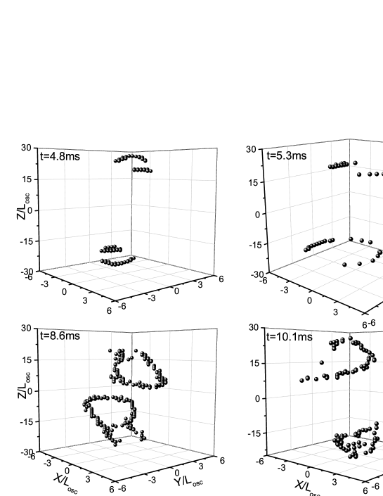
Figure 1: Typical vortex germs.

For longer modulation of the trapping potential, in the time interval $5<t<10$ ms, there arise the germs of vortex rings shown in Fig. 1. If the pumping is stopped at this stage, the germs survive during the time around $0.2$ s, which shows that they are metastable topological objects.

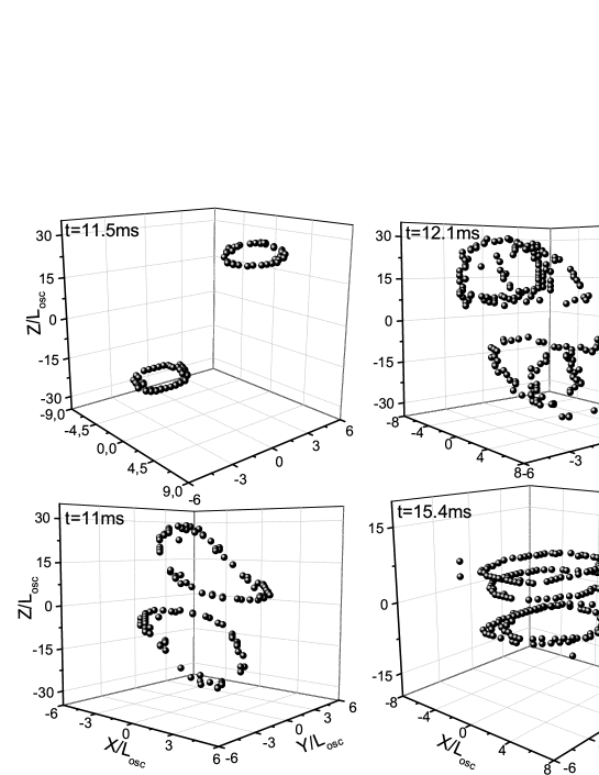
Figure 2: Typical vortex rings.

In the interval $10<t<15$ ms, well defined rings appear in pairs, with opposite circulations, so that their total circulation is zero. The circulation number for each ring is $\pm 1$. The corresponding picture is shown in Fig. 2. The ring lifetime, after switching off the pumping, is about $0.1$ s.

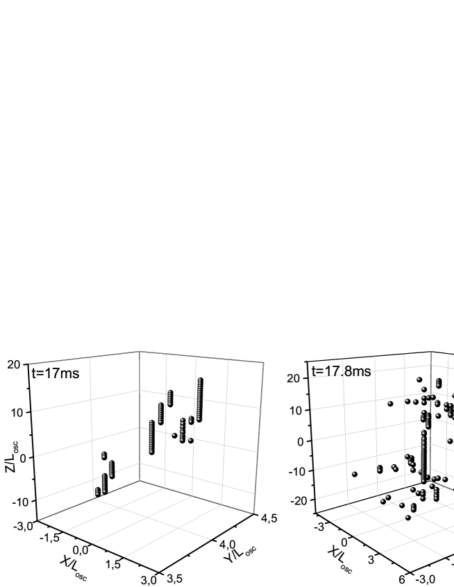
Figure 3: Almost straight vortex lines (left figure) and slightly deformed vortices (right figure).

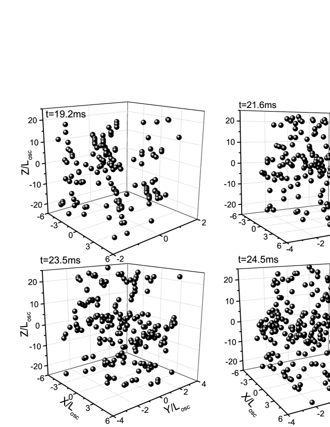
Figure 4: Strongly deformed vortices.

For $15<t<17$ ms, vortex lines arise (left Fig 3), with $\pm 1$ circulation number. The total circulation in the system is zero. A vortex lifetime is $0.2$ s. After $17$ ms, vortices start deforming, as in the right Fig. 3, and become strongly deformed in the interval $19<t<25$ ms, as is shown in Fig. 4.

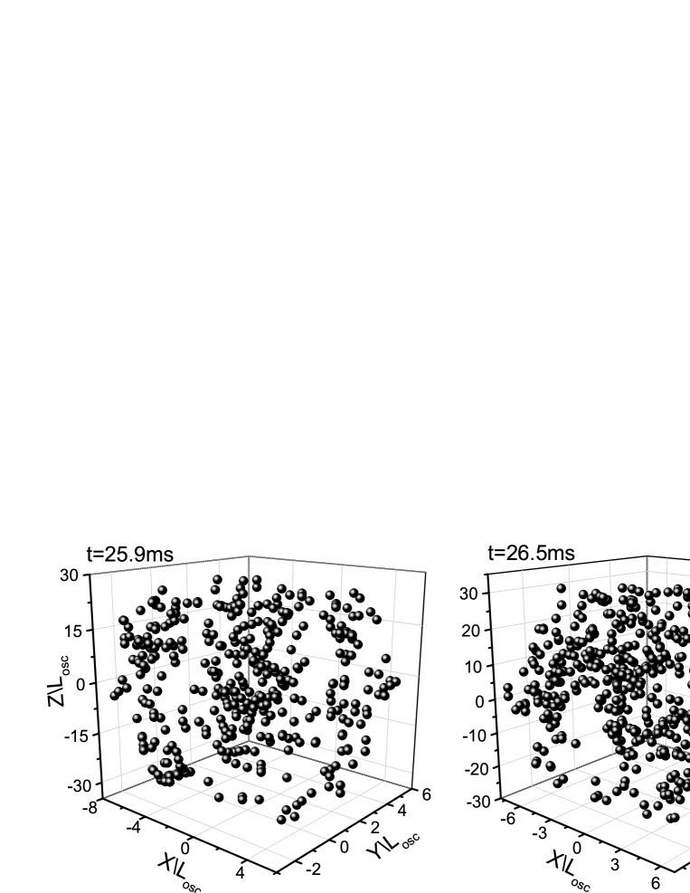
Figure 5: Initial stage of vortex turbulence.

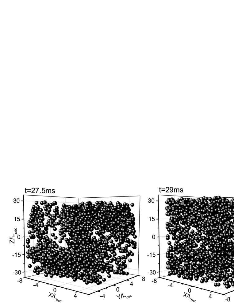
Figure 6: Developed vortex turbulence.

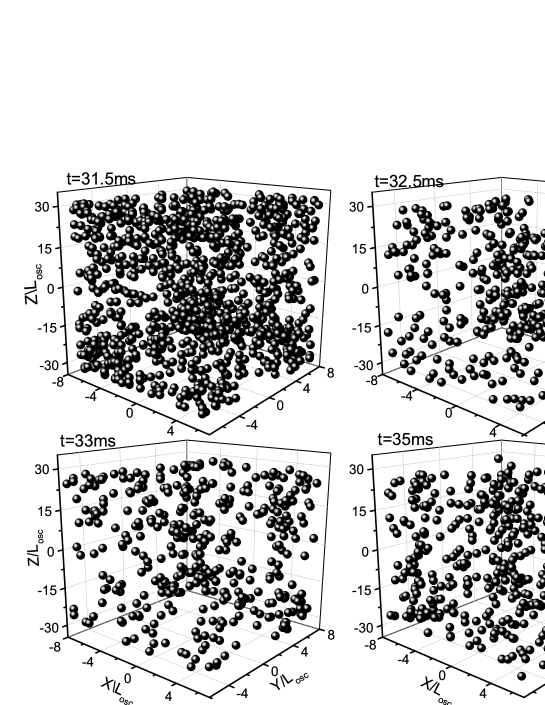
Figure 7: Decaying vortex turbulence.

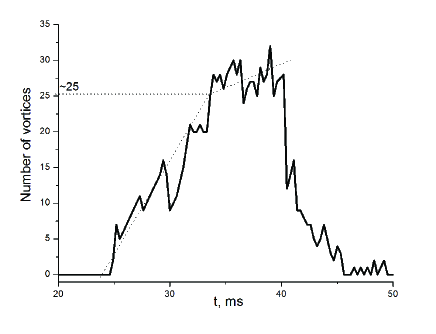
Figure 8: Number of vortices as a function of time.

In the time interval $25<t<27$ ms, the stage of vortex turbulence begins to develop, with strongly deformed and entangled vortices (Fig. 5). The dots in the figure are assumed to be connected with their nearest neighbours, which is rather difficult to draw, since the vortices are so strongly entangled and deformed. The turbulent regime becomes well developed after $27$ ms. The well developed turbulence exists approximately in the interval $27<t<30$ ms (Fig. 6), after which vortices start decaying (Fig. 7). The decaying turbulence occurs in the interval $30<t<40$ ms. Thus in total, the stage of quantum turbulence exists in the time interval $25<t<40$ ms. The state of quantum turbulence possesses the standard properties, typical of Vinen turbulence [15, 16, 17, 18, 19], such as the occurrence of a random vortex tangle and an anisotropic self-similar expansion preserving the aspect ratio of the cloud during its expansion. The number of vortices as a function of time, characterizing the beginning, development, and decay of turbulence, is shown in Fig. 8.

After about $45$ ms, the number of vortices quickly diminishes almost to zero and the granular, or droplet, state develops. In this state, the system is formed by dense droplets (grains) that are randomly distributed in space and surrounded by a rarified gas. The density inside a droplet is $100$ times larger than in the surrounding. The typical radius of a droplet is about $1.5\times 10^{-5}$ cm, which is close to the coherence length $\xi$. The phase inside a droplet is constant, while in the surrounding gas the phase is random, which implies that each droplet is a coherent object. The lifetime of a droplet, after switching off pumping, is much longer than the local equilibrium time,

$$t_{life}\sim 10^{-2}\;{\rm s}\gg t_{loc}\sim 10^{-3}\;{\rm s}\;,$$

which means that a droplet is a metastable formation. Generally, the droplet state has to satisfy the following properties in order to be classified as such. (1) the typical size of each droplet is of the order of the healing length; (2) the phase inside a droplet is constant, which defines a droplet as a coherent object; (3) the phase in the space around a droplet is random; (4) the lifetime of a droplet has to be much longer than the local equilibrium time; (5) the density inside a coherent droplet should be much larger than that of its incoherent surrounding. Under the considered pumping, the droplet state lasts approximately in the interval $40<t<150$ ms.

By the end of the droplet regime, after $150$ ms, the number of droplets falls and the regime of wave turbulence develops, where the system consists of small-amplitude waves of the density only three times larger than in the surrounding. The typical size of each wave is around $10^{-4}$ cm. The phase is everywhere random, so that there is no coherence either inside each wave or outside it. The density snapshots comparing the state of an equilibrium condensate with the droplet state and the state of wave turbulence is presented in Fig. 9.

3 Characteristic quantities

The appearance of this or that state is clearly connected with the amount of energy pumped into the system. The amount of energy transferred to the system depends on the amplitude of perturbation and on the duration of the perturbation time. It is, therefore, more convenient to distinguish different regimes not merely by the pumping time, but rather by the amount of the energy pumped into the system. The alternating external field mainly increases the kinetic energy of the system, as is seen from Fig. 10. Hence it is logical to introduce such characteristics that take into account the change in the system kinetic energy [20]. The change of kinetic energy can be connected with the effective temperature

$$T_{eff}=\frac{2}{3}\;\left(E_{kin}-E_{kin}^{eq}\right)=\frac{2}{3}\;\Delta E_{kin}$$ (7)

defined through the difference of the current-state kinetic energy and its value at equilibrium.

The states of such nonequilibrium systems as lasers are usually characterized by Fresnel number, which for a system of cylindrical shape of radius $R$ and length $L$ reads

$$F=\frac{A_{cross}}{\lambda L}=\frac{\pi R^{2}}{\lambda L}\;.$$ (8)

Here, under the wavelength, it is possible to assume the thermal wavelength

$$\lambda=\sqrt{\frac{2\pi}{mT_{eff}}}\;,$$ (9)

which results in the effective Fresnel number

$$F=\sqrt{\frac{\pi\alpha\Delta E_{kin}}{12\hbar\omega_{r}}}\;,$$ (10)

with the aspect ratio

$$\alpha\equiv\frac{\omega_{z}}{\omega_{r}}=\frac{4R^{2}}{L^{2}}\;.$$

Finally, it is possible to introduce the effective Mach number

$$M=\frac{v}{c}=\sqrt{\frac{2\Delta E_{kin}}{mc^{2}}}\;,$$ (11)

where $c$ is sound velocity. The classification of nonequilibrium states by means of the introduced characteristic quantities is illustrated in Fig. 11. Note that the developed regime of wave turbulence, where coherence completely disappears, corresponds to the effective temperature $T_{eff}=23.5\omega_{r}$, which practically coincides with the critical temperature $T_{c}=23.8\omega_{r}$ for ⁸⁷Rb in the studied setup.

4 Resonant generation

The frequency of the alternating field modulating the trap potential in the above setup was not connected to any transition frequency of the Bose system in the trap. If, however, the modulation frequency is specially tuned to the transition frequency between the ground state and an excited state representing a coherent topological mode, as described in Refs. [5, 6, 7], the beginning of the nonequilibrium process, for times $t\ll 100$ ms, can be different. This is illustrated in Figs. 12 and 13 by the temporal behaviour of the Fresnel number for different aspect ratios and different modulation amplitudes, with other parameters fixed as in all calculations above. In these figures, the parameter $b$ defines the ratio of the modulation amplitude to the strength of interactions between the atoms. The effective Fresnel number oscillates with time. The amplitude of the oscillations and their period increase with growing modulation amplitude $b$. In contrast, when $b$ is fixed and the aspect ratio increases, only the oscillation amplitude rises, while the oscillation period does not vary.

The resonant generation is possible only at the beginning of the pumping process, till times of order $10$ ms. For much larger times, the effect of power broadening comes into play, and the whole process of creation of nonequilibrium states continues approximately as under nonresonant pumping.

In conclusion, we demonstrated that strongly nonequilibrium states of Bose-Einstein condensates, containing topological modes, can be created by subjecting the system of trapped atoms to external alternating fields. The generated nonequilibrium states are conveniently characterized by effective temperature, Fresnel number, and Mach number.

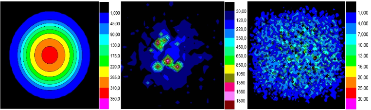
Figure 9: Density snapshot of equilibrium condensate (left plot), droplet state (middle plot), and wave turbulence (right plot).

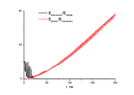
Figure 10: Comparison of kinetic and potential energies in the condensate of trapped atoms.

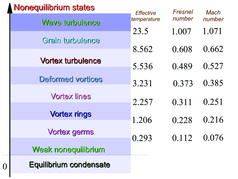
Figure 11: Classification of nonequilibrium states of trapped Bose-condensed atoms.

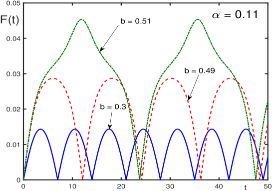
Figure 12: Temporal variation of Fresnel number for a fixed aspect ratio $\alpha$ and different modulation amplitudes, labeled by the parameter $b$.

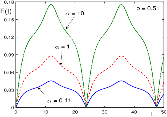
Figure 13: Temporal variation of Fresnel number for a fixed modulation amplitude and different values of aspect ratio.

References

- [1] Bogolubov N N 1949 Lectures on Quantum Statistics (Kiev: Ryadyanska Shkola).
- [2] Bogolubov N N 1967 Lectures on Quantum Statistics (New York: Gordon and Breach) Vol. 1.
- [3] Bogolubov N N 1970 Lectures on Quantum Statistics (New York: Gordon and Breach) Vol. 2.
- [4] Bogolubov N N 2015 Quantum Statistical Mechanics (Singapore: World Scientific).
- [5] Yukalov V I, Yukalova E P and Bagnato V S 1997 Phys. Rev. A 56 4845
- [6] Yukalov V I, Yukalova E P and Bagnato V S 2002 Phys. Rev. A 66 043602
- [7] Yukalov V I 2011 Phys. Part. Nucl. 42 460
- [8] Shiozaki R F, Telles G D, Yukalov V I and Bagnato V S 2011 Laser Phys. Lett. 8 393
- [9] Seman J A, Henn E A L, Shiozaki R F, Roati G, Poveda-Cuevas F J, Magalhães K M F, Yukalov V I, Tsubota M, Kobayashi M, Kasamatsu K and Bagnato V S 2011 Laser Phys. Lett. 8 691
- [10] Novikov A N, Yukalov V I and Bagnato V S 2015 J. Phys. Conf. Ser. 594 012040
- [11] Yukalov V I, Novikov A N and Bagnato V S 2014 Laser Phys. Lett. 11 095501
- [12] Yukalov V I, Novikov A N and Bagnato V S 2015 Phys. Lett. A 379 1366
- [13] Yukalov V I, Novikov A N and Bagnato V S 2015 J. Low Temp. Phys. 180 53
- [14] Yukalov V I, Novikov A N, Yukalova E P and Bagnato V S 2016 J. Phys. Conf. Ser. 691 012019
- [15] Vinen W F 2006 J. Low Temp. Phys. 145 7
- [16] Vinen W F 2010 J. Low Temp. Phys. 161 419
- [17] Tsubota M, Kobayashi M and Takeuchi H 2013 Phys. Rep. 522 191
- [18] Nemirovskii S K 2013 Phys. Rep. 524 85
- [19] Tsatsos M C, Tavares, P E S, Cidrim A, Fritsch A R, Caracanhas M A, Dos Santos F E A, Barenghi C F and Bagnato V S 2016 Phys. Rep. 622 1
- [20] Yukalov V I, Novikov A N and Bagnato V S 2018 Laser Phys. Lett. 15 065501