Kalman Filter-based Head Motion Prediction for Cloud-based Mixed Reality

Abstract.

Volumetric video allows viewers to experience highly-realistic 3D content with six degrees of freedom in mixed reality (MR) environments. Rendering complex volumetric videos can require a prohibitively high amount of computational power for mobile devices. A promising technique to reduce the computational burden on mobile devices is to perform the rendering at a cloud server. However, cloud-based rendering systems suffer from an increased interaction (motion-to-photon) latency that may cause registration errors in MR environments. One way of reducing the effective latency is to predict the viewer’s head pose and render the corresponding view from the volumetric video in advance.

In this paper, we design a Kalman filter for head motion prediction in our cloud-based volumetric video streaming system. We analyze the performance of our approach using recorded head motion traces and compare its performance to an autoregression model for different prediction intervals (look-ahead times). Our results show that the Kalman filter can predict head orientations $0.5\text{\,}\mathrm{d}\mathrm{e}\mathrm{g}\mathrm{r}\mathrm{e}\mathrm{e}\mathrm{s}$ more accurately than the autoregression model for a look-ahead time of $60\text{\,}\mathrm{m}\mathrm{s}$.

1. Introduction

With the advances in volumetric capture technologies, volumetric video has been gaining importance for the immersive representation of 3D scenes and objects for virtual reality (VR) and augmented reality (AR) applications (Schreer et al., 2019b). Combined with highly accurate positional tracking technologies, volumetric video allows users to freely explore six degrees of freedom (6DoF) content and enables novel mixed reality (MR) applications where highly realistic virtual objects can be placed inside real environments and animated based on user interaction (Eisert and Hilsmann, 2020).

Geometry of volumetric objects is usually represented using meshes or point clouds. High-quality volumetric meshes typically contain thousands of polygons, and high-quality point clouds may contain millions to billions of points (Schreer et al., 2019a; Schwarz et al., 2019). Therefore, rendering complex volumetric content is still a very demanding task despite the remarkable computing power available in today’s mobile devices (Clemm et al., 2020). Moreover, no efficient hardware implementations of mesh/point cloud decoders are available yet. Software-based decoding can be prohibitively expensive in terms of battery usage and may not be able to meet the real-time rendering requirements (Qian et al., 2019).

One way to avoid the complex rendering on mobile devices is to offload the processing to a powerful remote server which dynamically renders a 2D view from the volumetric video based on the user’s actual head pose (Shi and Hsu, 2015). The server then compresses the rendered texture into a 2D video stream and transmits it over a network to the client. The client can then efficiently decode the video stream using its hardware decoder and display the dynamically updated content to the viewer. Moreover, the cloud-based rendering approach allows utilizing highly efficient 2D video coding techniques and thus can reduce the network bandwidth requirements by avoiding the transmission of the volumetric content (Qian et al., 2019).

However, one drawback of cloud-based rendering is the increased interaction latency, also known as the motion-to-photon (M2P) latency (Shi et al., 2012). Due to the network round-trip time and the added processing delays, the M2P latency is higher than in a system that performs the rendering locally. Several studies show that an increased interaction latency may lead to a degraded user experience and motion sickness (Beigbeder et al., 2004; McCandless et al., 2000; Livingston and Ai, 2008).

One way to reduce the latency is to predict the user’s future head pose at the cloud server and render the corresponding view of the volumetric content in advance. Thereby, it is possible to significantly reduce or even eliminate the M2P latency, if the user pose is successfully predicted for a look-ahead time (LAT) equal to or larger than the M2P latency of the system. However, mispredictions of head motion may increase registration errors and degrade the user experience in AR environments (Livingston and Ai, 2008). Therefore, designing accurate head motion prediction algorithms is crucial for high-quality volumetric video streaming.

In this paper, we consider the problem of head motion prediction for cloud-based AR/MR applications. Our main contributions are as follows:

• We develop a Kalman filter-based predictor for head motion prediction in 6DoF space and analyze its performance compared to an autoregression model and a baseline (no prediction) model using recorded head motion traces.

• We present an architecture for integration of the Kalman filter-based predictor into our existing cloud-based volumetric streaming framework.

The paper is structured as follows. Sec. 2 gives an overview of the literature on volumetric video streaming, remote rendering and head motion prediction. Sec. 3 gives an overview of our cloud-based volumetric video streaming system. Sec. 4 describes the developed Kalman filter-based predictor and presents a framework for its integration into our volumetric streaming system. Sec. 5 presents our experimental setup and the evaluation results. Sec. 6 concludes this paper.

2. Related Work

2.1. Volumetric video streaming

A few recent works deal with efficient streaming of volumetric videos in different content representations. Hosseini and Timmerer (Hosseini and Timmerer, 2018) extended the concepts of Dynamic Adaptive Streaming over HTTP (DASH) for point cloud streaming. They proposed different approaches for spatial subsampling of dynamic point clouds to decrease the density of points in the 3D space and thus reduce the bandwidth requirements. Park et al. (Park et al., 2019) proposed using 3D tiles for streaming of voxelized point clouds. Their system selects 3D tiles and adjusts the corresponding level-of-details (LODs) using a rate-utility model that considers the user’s viewpoint and distance to the object. Qian et al. (Qian et al., 2019) developed a point cloud streaming system that uses an edge proxy to convert point cloud streams into 2D video streams based on the user’s viewpoint in order to enable efficient decoding on mobile devices. They also proposed various optimizations to reduce the M2P latency between the client and the edge proxy. Van der Hooft et al. (van der Hooft et al., 2019) proposed an adaptive streaming framework compliant to the recent point cloud compression standard MPEG V-PCC (Schwarz et al., 2019). Their framework PCC-DASH enables adaptive streaming of scenes with multiple dynamic point cloud objects. They also presented rate adaptation techniques that rely on the user’s position and focus as well as the available bandwidth and the client’s buffer status to select the optimal quality representation for each object. Petrangeli et al. (Petrangeli et al., 2019) proposed a streaming framework for AR applications that dynamically decides which virtual objects should be fetched from the server as well as their LODs, depending on the proximity of the user and likelihood of the user to view the object.

2.2. Remote rendering

The idea of offloading the rendering process to a powerful remote server was first considered in 1990s when PCs did not have sufficient computational power for intensive graphics tasks (Shi and Hsu, 2015). A remote rendering system renders complex graphics on a powerful server and delivers the result over a network to a less-powerful client device.

With the advent of cloud gaming and Mobile Edge Computing (MEC), interactive remote rendering applications have started to emerge which allow the client device to control the rendering application based on user interaction (Mangiante et al., 2017; Shi et al., 2019; Qian et al., 2019). Mangiante et al. (Mangiante et al., 2017) presented a MEC system for field-of-view (FoV) rendering of $360\mathrm{°}$ videos to optimize the required bandwidth and reduce the processing requirements and battery utilization. Shi et al. (Shi et al., 2019) developed a MEC system to stream AR scenes containing only the user’s FoV plus a latency-adaptive margin around it. They deployed the prototype on a MEC node connected to a LTE network and evaluated its performance. A detailed survey of interactive remote rendering system is given in (Shi and Hsu, 2015).

2.3. Head motion prediction

Previous techniques for head motion prediction were mainly developed for dealing with the rendering and display delays of the early AR systems. In his dissertation, Azuma (Azuma, 1995) developed an AR system that relies on head motion prediction to reduce the dynamic registration errors of virtual objects. His results indicate that prediction is most effective for short prediction intervals that are less than $80\text{\,}\mathrm{m}\mathrm{s}$. In a follow-up work, Azuma and Bishop (Azuma and Bishop, 1995) presented a frequency domain analysis of head motion prediction and concluded that the error in predicted position grows rapidly with increasing prediction intervals and head motion signal frequencies. Van Rhijn et al. (van Rhijn et al., 2005) proposed a framework for Bayesian predictive filtering algorithms and studied the effect of the filter parameters on the prediction performance. They compared the performances of different prediction methods using both synthetic and experimental data. La Viola (LaViola, 2003) presented a comparison of the unscented Kalman filter (UKF) and extended Kalman filter (EKF) for prediction of head and hand orientation represented with quaternions. Kraft (Kraft, 2003) proposed a quaternion-based UKF that extends the original UKF formulation to address the inherent properties of unit quaternions. The developed filter was applied for prediction of head orientation; however, the evaluation is limited to simulated motion. Himberg and Motai (Himberg and Motai, 2009) proposed an EKF that operates on the change of quaternions between consecutive time points (delta quaternion) and showed that their approach provides similar prediction performance to a quaternion-based EKF with less computational burden.

In recent years, with the resurgence of interest in VR, head motion prediction regained importance for prediction of the future user viewport in $360\mathrm{°}$ videos. Bao et al. (Bao et al., 2016) developed regression models to predict the user’s viewport. They also used the same models to predict the accuracy of prediction to determine the size of margins around the viewport for efficient transmission of $360\mathrm{°}$ videos. Sanchez et al. (de la Fuente et al., 2019) proposed angular velocity and angular acceleration based predictors to tackle the delay issue in tile-based viewport-dependent streaming. Qian et al. (Qian et al., 2018) analyzed the performance of several machine learning algorithms on head movement traces collected from 130 diverse users and employed different prediction algorithms depending on the prediction interval. The developed prediction framework was integrated into a streaming system for $360\mathrm{°}$ videos to reduce the bandwidth usage or boost the video quality given the same bandwidth.

The principles of head motion prediction for $360\mathrm{°}$ videos and volumetric videos in mixed reality are similar. However, volumetric videos are more complex and allow movement in a higher degree of freedom making prediction a more difficult task. In our volumetric streaming system, we employ a Kalman filter-based prediction framework to jointly predict both translational and rotational head movements in 6DoF space.

3. Volumetric streaming system

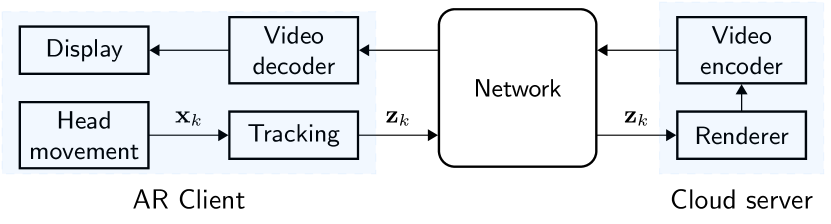
Figure 1. High level operation of our cloud-based volumetric streaming system.

Fig. 1 shows an overview of our cloud-based volumetric streaming system. We abstract the software components as functional blocks to focus on the prediction aspects. A detailed software architecture of our system is described in (ano, [n.d.]).

At the cloud server, we store our compressed volumetric video as a single MP4 file containing video and mesh tracks. Particularly, we encode the texture atlas using H.264/AVC and the mesh geometry using Google Draco that implements the Edgebreaker algorithm (Rossignac, 1999). The compressed mesh and texture data are multiplexed into different tracks of an MP4 file ready to be processed by the game engine (Unity) running at our server by means of a native plug-in that demultiplexes and decodes the respective data streams.

Head movement of the user is described by the state vector $\mathbf{x}_{k}$. The tracking system of the AR headset measures the head pose with a sampling interval of $t_{s}$. The measurement $\mathbf{z}_{k}$ is then sent over a network to the cloud server, which then renders the corresponding view from the volumetric content (textured meshes) according to $\mathbf{z}_{k}$. Next, the rendered view is encoded as a video stream using the NVIDIA hardware encoder (NVENC) (NVIDIA, 2019) and sent to the client using WebRTC (Cullen Jennings, 2019). We selected WebRTC as the delivery protocol since it provides low-latency (real-time) streaming capabilities and is already widely adopted by different web browsers allowing our system to support several different platforms. After the transmission, the client decodes the received video stream and displays it to the viewer.

The time period between the head movement and display of the decoded video frame to the viewer is the M2P latency of the system which we aim to compensate by applying prediction.

4. Head motion prediction

We propose to use a Kalman filter for 6DoF head motion prediction in our cloud-based volumetric streaming system. As a benchmark, we investigate the performance of a Baseline and an autoregression model.

4.1. Baseline

The Baseline model represents the operation of the system without prediction. We assume that the prediction time is set equal to the M2P latency such that the prediction completely eliminates the latency. For a prediction time of $N$ samples, the measurement $\mathbf{z}_{k}$ is simply propagated $N$ samples ahead in our simulations and set as the user pose at time $k+N$, i.e. $\hat{\mathbf{x}}_{k+N}=\mathbf{z}_{k}$.

4.2. Autoregression

Autoregressive (AutoReg) models use a linear combination of the past values of a variable to forecast its future values (Hyndman and Athanasopoulos, 2018).

An AutoReg model of lag order $\rho$ can be written as

(1) $$y_{t}=c+\phi_{1}y_{t-1}+\phi_{2}y_{t-2}+\dots+\phi_{\rho}y_{\rho-1}+\epsilon_{t}$$

where $y_{t}$ is the true value of the time series $y$ at time $t$, $\epsilon_{t}$ is the white noise, $\phi_{i}$ are the coefficients of the model. Such a model with $\rho$ lagged values is referred to as an $\mathrm{AR}(\rho)$ model. The optimal lag order for the model can be automatically determined using statistical tests such as the Akaike Information Criterion (AIC) (Akaike, 1973). AutoReg models must first be trained to learn the model coefficients, and the learned model coefficients $\phi_{i}$ as well as the lag order $\rho$ may vary depending on the training data.

Typically, we need to predict not only the next sample but multiple samples ahead in the future to achieve a given look-ahead time (LAT). Therefore, we repeat the prediction step in a sliding window fashion by using the just-predicted sample for the prediction of the next sample and iterate Eq. (1) until we achieve the desired LAT. Fig. 2 shows an example that demonstrates the iterations of the AutoReg model for a history window of 3 samples and LAT =2.

.

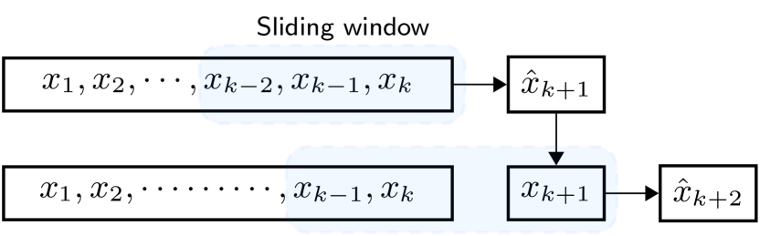
Figure 2. An example showing multi-step ahead prediction using autoregression model for a history window of 3 and a look-ahead time (LAT)of 2 samples.

4.3. Kalman filter

Basics

The Kalman filter estimates the state $\mathbf{x}\in\mathbb{R}^{n}$ of a discrete-time process expressed by the linear difference equation

(2) $$\mathbf{x}_{k}=\mathrm{\mathbf{F}}\mathbf{x}_{k-1}+\mathbf{w}_{k-1},$$

with a measurement (observation) $\mathbf{z}\in\mathbb{R}^{m}$ expressed by

(3) $$\mathbf{z}_{k}=\mathrm{\mathbf{H}}\mathbf{x}_{k}+\mathbf{v}_{k},$$

where the random variables $\mathbf{w}_{k}$ and $\mathbf{v}_{k}$ represent the process and measurement noise, respectively. They are assumed to be independent from each other and have the Gaussian distributions $\mathit{p}(\mathbf{w})\sim\mathit{N}(0,\mathrm{\mathbf{Q}})$ and $\mathit{p}(\mathbf{v})\sim\mathit{N}(0,\mathrm{\mathbf{R}})$ where $\mathrm{\mathbf{Q}}$ and $\mathrm{\mathbf{R}}$ are the process and measurement noise covariance matrices, respectively. The general formulation of the Kalman filter allows $\mathrm{\mathbf{Q}}$ and $\mathrm{\mathbf{R}}$ to be changed at each time step; however, we assume that they remain constant. The matrix $\mathrm{\mathbf{F}}\in\mathbb{R}^{n\times n}$ represents the state transition (process) model that relates the state at the previous time step $\mathbf{x}_{k-1}$ to the current state $\mathbf{x}_{k}$. The matrix $\mathrm{\mathbf{H}}\in\mathbb{R}^{m\times n}$ represents the observation model that relates the state to the measurement. Since no external control is involved in a subject’s head movements, we do not include a control input in our framework (Welch and Bishop, 1995).

Given the knowledge of the state before step $k$, we define $\hat{\mathbf{x}}_{k}^{\mathchar 45\relax}$ as our a priori state estimate, and given the measurement $\mathbf{z}_{k}$ at step $k$, we define $\hat{\mathbf{x}}_{k}$ as our a posteriori state estimate. We can then define a priori estimate error and a posteriori estimate error as

(4) $$\mathrm{\mathbf{P}}_{k}^{\mathchar 45\relax} =\mathrm{cov}(\mathbf{x}_{k}-\hat{\mathbf{x}}_{k}^{\mathchar 45\relax}),$$

(5) $$\mathrm{\mathbf{P}}_{k} =\mathrm{cov}(\mathbf{x}_{k}-\hat{\mathbf{x}}_{k}),$$

respectively.

A complete Kalman filter cycle consists of the time update (”prediction”) and measurement update (”correction”) steps. The time update projects the current state estimate ahead in time using the process model $\mathrm{\mathbf{F}}$. Given the previous state estimate $\hat{\mathbf{x}}_{k-1}$, the a priori state and error covariance estimates are obtained by

(6) $$\hat{\mathbf{x}}_{k}^{\mathchar 45\relax} =\mathrm{\mathbf{F}}\hat{\mathbf{x}}_{k-1},$$

(7) $$\mathrm{\mathbf{P}}_{k}^{\mathchar 45\relax} =\mathrm{\mathbf{F}}\mathrm{\mathbf{P}}_{k-1}\mathrm{\mathbf{F}}^{T}+\mathrm{\mathbf{Q}},$$

respectively.

The measurement update applies a correction to the projected estimate using the actual measurement. First, the Kalman gain $\mathrm{\mathbf{K}}$ is computed which is a ratio expressing how much the filter ”trusts” the prediction vs. the measurement

(8) $$\mathrm{\mathbf{K}}_{k}=\mathrm{\mathbf{P}}_{k}^{\mathchar 45\relax}\mathrm{\mathbf{H}}^{T}(\mathrm{\mathbf{H}}\mathrm{\mathbf{P}}_{k}^{\mathchar 45\relax}\mathrm{\mathbf{H}}^{T}+\mathrm{\mathbf{R}})^{-1}.$$

Then, the actual measurement $\mathbf{z}_{k}$ is incorporated to obtain the a posteriori state estimate by

(9) $$\mathbf{\hat{x}}_{k}=\mathbf{\hat{\mathbf{x}}}_{k}^{\mathchar 45\relax}+\mathrm{\mathbf{K}}_{k}(\mathbf{z}_{k}-\mathrm{\mathbf{H}}\hat{\mathbf{x}}_{k}^{\mathchar 45\relax}),$$

and the a posteriori error covariance is obtained by

(10) $$\mathrm{\mathbf{P}}_{k}=(\mathrm{\mathbf{I}}-\mathrm{\mathbf{K}}_{k}\mathrm{\mathbf{H}})\mathrm{\mathbf{P}}_{k}^{\mathchar 45\relax}.$$

A detailed derivation of the Kalman filter equations can be found in (Labbe, 2015).

Filter design

We use a 14D state vector that consists of the position and orientation components as well as their first time-derivatives

(11) $$\mathbf{x}=\left[x,\dot{x},y,\dot{y},z,\dot{z},q_{w},\dot{q_{w}},q_{x},\dot{q_{x}},q_{y},\dot{q_{y}},q_{z},\dot{q_{z}}\right]^{T}.$$

We initialize the state as a zero-vector, $\mathbf{x}=\mathrm{\mathbf{0}}_{14}$ and the error covariance as an identity matrix, $\mathrm{\mathbf{P}}=\mathrm{\mathbf{I}}_{14}$. Our state transition model $\mathrm{\mathbf{F}}\in\mathbb{R}^{14\times 14}$ is a block diagonal matrix with the block

$$\begin{bmatrix}1&\Delta t\\ 0&1\end{bmatrix}$$

repeated seven times in the diagonal such that the same constant-velocity motion model is applied to all the state variables. $\Delta t$ is the time step of the filter set equal to the sampling time $t_{s}$ ($5\text{\,}\mathrm{m}\mathrm{s}$) in our simulations. Our observation model $\mathrm{\mathbf{H}}\in\mathbb{R}^{7\times 14}$ is also a block diagonal matrix with $\begin{bmatrix}1&0\end{bmatrix}$ repeated seven times in the diagonal.

Measurement noise

$\mathrm{\mathbf{R}}\in\mathbb{R}^{7\times 7}$ models the noise in the sensors as a covariance matrix. The AR headset we use for data collection, Microsoft HoloLens, uses advanced visual-inertial Simultaneous Localization and Mapping (SLAM) algorithms that track the user pose with high accuracy (Liu et al., 2018). Therefore, we experimented with small noise variances and empirically constructed $\mathrm{\mathbf{R}}$ as a diagonal matrix with the diagonal values set to $10^{-6}$. In practice, there might be correlation between different sensors and usually their noise is not a pure Gaussian (Labbe, 2015). However, for the lack of a better sensor model, we employ a simplified measurement matrix.

Process noise

Since we have a discrete-time process in which we sample the system at regular intervals, we need a discrete representation of the noise term $\mathbf{w}$ given in Eq. 2. Therefore, we consider a discretized white noise model which assumes that the velocity remains constant during each $\Delta t$ but differs for each time period (Bar-Shalom et al., 2004).

The process noise covariance matrix $\mathrm{\mathbf{Q}}\in\mathbb{R}^{14\times 14}$ is then a block diagonal matrix with the block

$$\begin{bmatrix}\frac{\Delta t^{4}}{4}&\frac{\Delta t^{3}}{2}\\[5.0pt] \frac{\Delta t^{3}}{2}&\Delta t^{2}\end{bmatrix}\sigma_{\nu}^{2}$$

repeated seven times in the diagonal, where the noise variance is empirically set to $\sigma_{\nu}^{2}=10^{3}$ for the first three blocks (position) and $\sigma_{\nu}^{2}=4\times 10^{6}$ for the remaining blocks (orientation). A derivation of $\mathrm{\mathbf{Q}}$ for the discretized white noise model is given in (Bar-Shalom et al., 2004).

Multi-step ahead prediction

Each iteration of the Kalman filter results in an a posteriori state estimate $\mathbf{\hat{x}}_{k}$. To obtain an $N$-step prediction $\mathbf{\hat{x}}_{k+N}$, after each iteration we need to propagate $\mathbf{\hat{x}}_{k}$ ahead by applying the process model $\mathrm{\mathbf{F}}$ multiple times on $\mathbf{\hat{x}}_{k}$, i.e. by iterating the Eq. (6) $N$ times (Kiruluta et al., 1997; van Rhijn et al., 2005).

4.4. Representation of orientation

We perform the prediction of orientations in the quaternion domain (Diebel, 2006). We readily obtain quaternions from the HoloLens and thus can avoid conversion from another representation such as Euler angles or rotation matrices. Quaternions allow smooth interpolation of orientations using techniques like Spherical Linear Interpolation of Rotations (SLERP) (Shoemake, 1985). Moreover, quaternions do not suffer from gimbal lock as opposed to Euler angles and offer a singularity-free description of orientation. They are more compact compared to rotation matrices and thus computationally more efficient (Jia, 2013). The set of unit quaternions, i.e. quaternions of norm one, constitutes a unit sphere in 4-D space. The three remaining degrees of freedom after applying the unity constraint are sufficient to represent any rotation in 3-D space (Diebel, 2006).

4.5. System integration

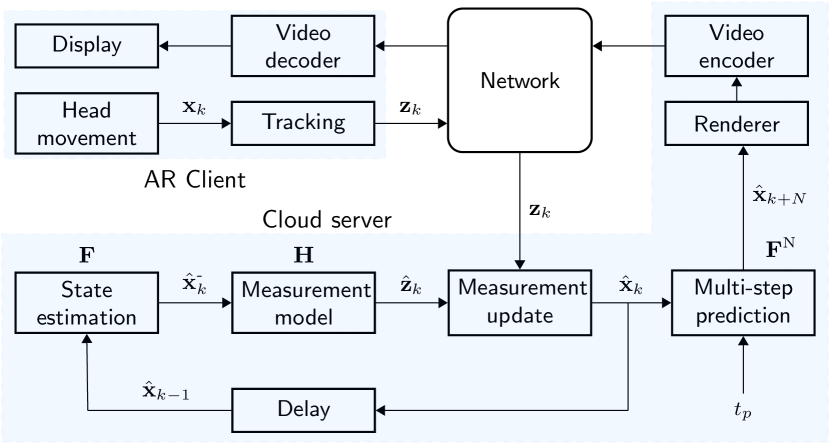
Figure 3. Integration of the Kalman filter-based predictor into our cloud-based volumetric streaming system.

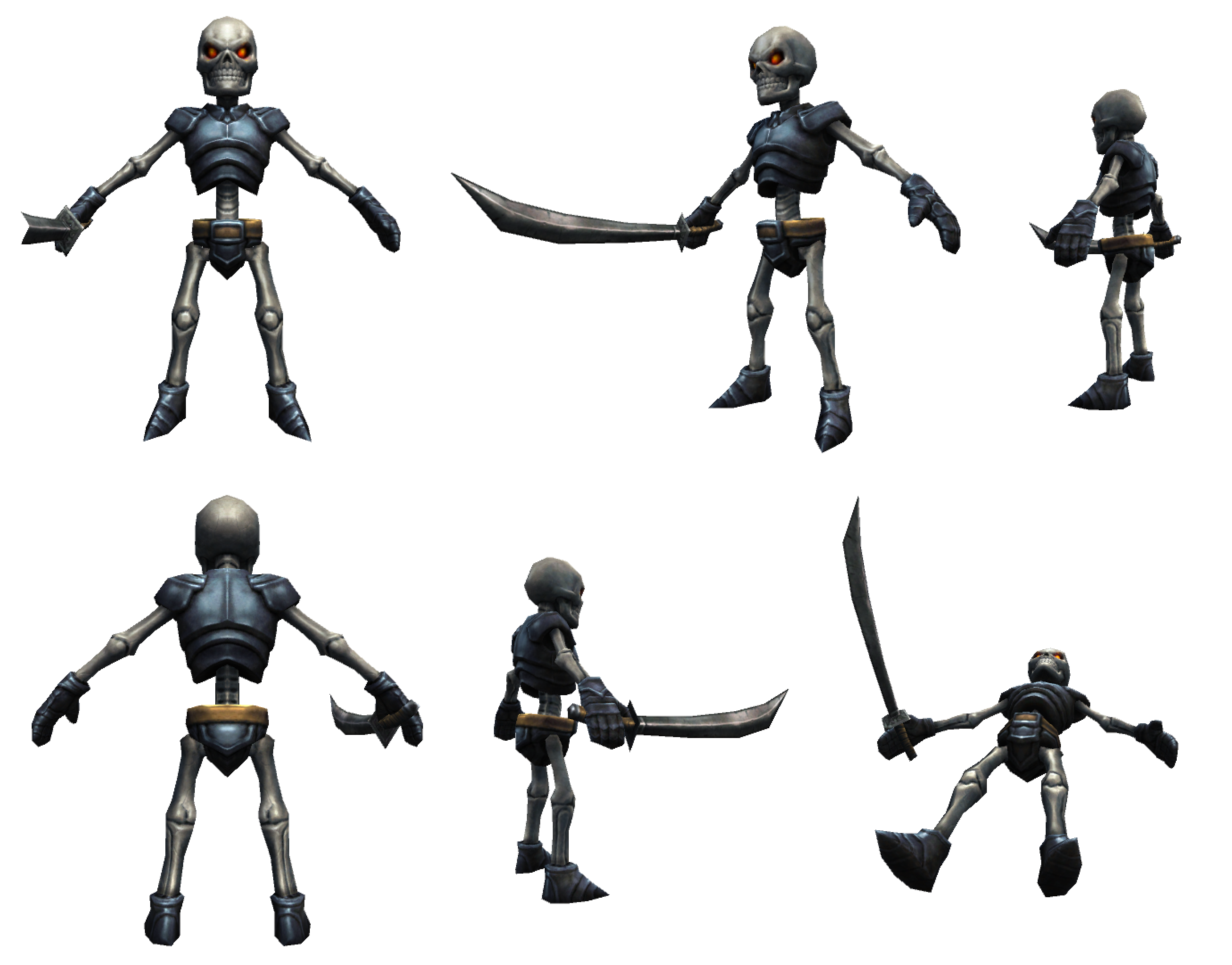
Figure 4. The virtual object used during trace collection shown from different viewpoints.

Figure 5. One sample trace from our dataset collected using Microsoft HoloLens. Top: position, bottom: orientation (shown as Euler angles).

Fig. 3 shows the different steps of the Kalman filter-based predictor and presents interfaces for its integration into our volumetric streaming system. After initialization, the state estimate from the previous step $\hat{\mathbf{x}}_{k-1}$ is propagated in time using the process model $\mathrm{\mathbf{F}}$ and the time step of the filter $\Delta t=1/f_{s}$. Then, the obtained initial state estimate $\hat{\mathbf{x}}_{k}^{\mathchar 45\relax}$ is converted to a measurement estimate $\hat{\mathbf{z}}_{k}$ using the measurement model $\mathrm{\mathbf{H}}$. Finally, the actual measurement $\mathbf{z}_{k}$ (sent over the network) is combined with $\hat{\mathbf{z}}_{k}$ to obtain the corrected state estimate $\hat{\mathbf{x}}_{k}$. This completes one cycle of the Kalman filter operation. At the end of each cycle, the process model $\mathrm{\mathbf{F}}$ is re-used to propagate the state estimate $\hat{\mathbf{x}}_{k}$ in time by the $\mathrm{LAT}=t_{\mathrm{p}}$ and obtain the predicted state $\hat{\mathbf{x}}_{k+N}$ at time $t_{k}+t_{p}$. Finally, a corresponding view from the volumetric video is rendered based on the predicted user pose and transmitted to the client.

5. Evaluation

To evaluate the proposed predictors for different head movements and LATs, we recorded user traces via Microsoft HoloLens and created a Python-based simulation framework that enables offline processing of the traces. Below, we first discuss the experimental setup and the evaluation metrics, before presenting the obtained results and discussing the limitations of our approach.

5.1. Experimental setup

Dataset

We created a HoloLens application that overlays a virtual object (shown in Fig. 4) on the real world and collected 14 head movement traces. For each session, the user was asked to freely move around and explore the object for a duration of $60\text{\,}\mathrm{s}$. We recorded the position samples ($x$, $y$, $z$) and rotation samples in the form of quaternions ($q_{x}$, $q_{y}$, $q_{z}$, $q_{w}$) together with the corresponding timestamps. Since the raw sensor data we obtained from the HoloLens was unevenly sampled at $60\text{\,}\mathrm{H}\mathrm{z}$ (i.e. different temporal distances between consecutive samples), we interpolated the data to obtain temporally equidistant samples. We upsampled the position data using linear interpolation and quaternions using SLERP (Shoemake, 1985). Thus, we obtained an evenly-sampled dataset with a sampling rate of $200\text{\,}\mathrm{H}\mathrm{z}$. This resampling significantly simplifies the offline analysis of our traces and implementation of the predictors.

Autoregression model settings

We used one of our collected head motion traces (see Sec. 5.1) as training data and estimated the AutoReg model parameters from each time series ($x$, $y$, $z$, $q_{w}$, $q_{x}$, $q_{y}$, $q_{z}$) separately using the Python library statsmodels (Seabold and Perktold, 2010). To select the best AutoReg model, we trained different models using three different training traces and selected the best-performing model. Our models have an automatically determined lag order of 40 samples, i.e. they consider the past $40*5=200$ ms and predict the next sample using Eq. (1).

5.2. Trace statistics

Fig. 5 shows one of the traces in our dataset. For visualization purposes, orientations are given as Euler angles (yaw, pitch, roll), although we perform the prediction in the quaternion domain (see Sec. 4.4). Note that our framework uses a left-handed coordinate system where +y axis points up and +z axis lies in the viewing direction.

We can make two important observations based on the sample trace: firstly, the viewer rarely moves along the y-axis (except for the time period between $3842\text{\,}\mathrm{s}$ during which the viewer probably sat down and stood back up), which is understandable since it requires more effort to crouch down and stand up. Secondly, the orientation changes are typically due to yaw movements, whereas the magnitude of changes due to roll and pitch movements are much smaller. Our observations are also confirmed by visual inspection of the other recorded traces.

Head movement velocity

We analyzed the peak and mean head movement velocities by computing the first-order difference for all degrees of freedom ($x$, $y$, $z$, yaw, roll, pitch). Since numerical differentiation using finite-differences is a noisy operation that amplifies any noise present in the data (Chartrand, 2011), we used a Savitzky-Golay filter (Savitzky and Golay, 1964) to smooth the computed velocities.

Fig. 6 shows the cumulative distribution functions (CDFs) of the computed linear and angular velocities, respectively, for trace 1 (shown in Fig. 5). We observe that the 95th percentile in $y$ dimension is located at $0.2\text{\,}\mathrm{m}\mathrm{/}\mathrm{s}$, whereas the 95th percentiles in $x$ and $z$ dimension are at around $0.5\text{\,}\mathrm{m}\mathrm{/}\mathrm{s}$. We also observe that the pitch and roll velocities are mostly smaller than the yaw velocity, which can reach peak values around $200\text{\,}\mathrm{d}\mathrm{e}\mathrm{g}\mathrm{/}\mathrm{s}$.

Fig. 7 shows the mean linear and angular velocities as well as the 95th percentile ranges for five different traces. In all traces, we observe that the linear velocities in $x$ and $z$ dimensions are greater than those in $y$. Similarly, the angular velocities in yaw dimension are greater than those in pitch and roll. Deviations from the mean values can be significant in all dimensions, as observed by inspecting the 95th percentiles (lightly shaded in the figure).

.

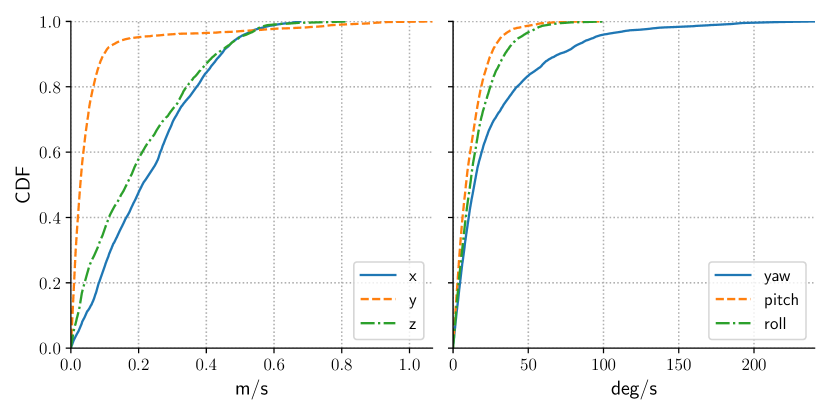
Figure 6. CDF of linear velocity (left) and angular velocity (right) for trace 1.

.

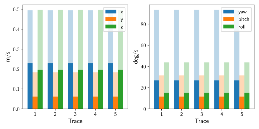
Figure 7. Mean linear velocity (left) and mean angular velocity (right) for five traces. Lighter shades show the 95th percentile.

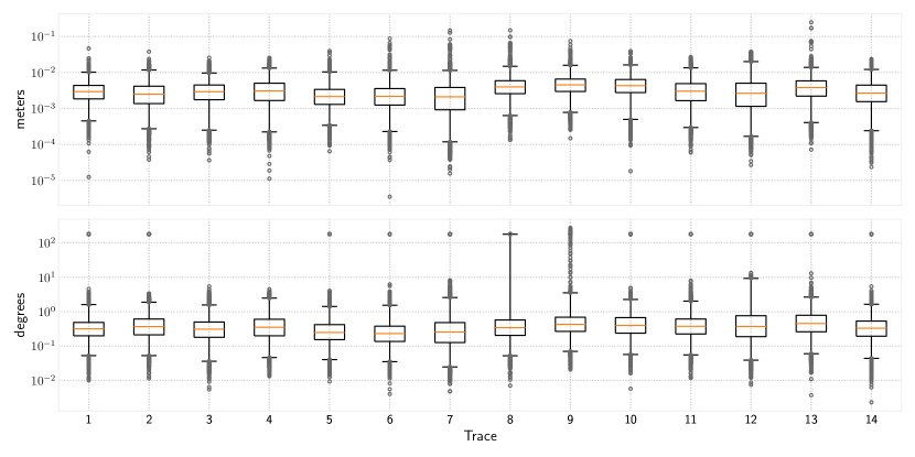
Figure 8. Per-trace distribution of the position errors (top) and angular errors (bottom) of the Kalman filter for a given LAT=60 ms. Whiskers represent the 1-99% range; outliers are shown by circles. Each trace contains 12k data points. Note the logarithmic scale of the y-axes.

5.3. Evaluation metrics

For evaluation of the prediction methods, we employed two objective error metrics: position error and angular error. Position error is the Euclidean distance (in meters) between the actual and the predicted position. It is defined as

(12) $$d=\sqrt{(\hat{x}-x)^{2}+(\hat{y}-y)^{2}+(\hat{z}-z)^{2}}.$$

Angular error is the spherical distance (in degrees) between the actual and the predicted orientation. Let $\mathbf{q}$ be a measured and $\mathbf{\hat{q}}$ be a predicted unit quaternion. Then, the spherical distance $\phi$ between the two orientations can be computed as follows (Solà, 2017)

(13) $$\mathbf{r} =\mathbf{q^{*}}\mathbf{\hat{q}}$$

(14) $$\phi =2\frac{180}{\pi}\arccos(r_{w})$$

where $\mathbf{q^{*}}$ is the conjugate of the quaternion $\mathbf{q}$ and $r_{w}$ is the scalar (real) part of the quaternion $\mathbf{r}$.

After computing the position and angular error for each time point, we compute the mean absolute error (MAE) over a trace as

(15) $$\mathrm{MAE(d)}=\frac{1}{N}\sum_{i=1}^{N}d_{i},\;\;\mathrm{MAE(\phi)}=\frac{1}{N}\sum_{i=1}^{N}\phi_{i}$$

where $d_{i}$ and $\phi_{i}$ are the position and angular errors at time $i$, respectively, and $N$ is the number of predicted samples in a trace.

5.4. Prediction results

We evaluated the performance of our Kalman filter-based predictor for different LATs {20,40,60,80,100} ms. This range was chosen considering the measured M2P latency of our cloud-based volumetric streaming system. Running our server on an Amazon Web Services (AWS) instance, we measured an average M2P latency around 60 ms with a network latency of 13.3 ms (ano, [n.d.]).

First, we evaluate the performance of the Kalman filter for a fixed LAT, $t_{p}=60$ ms. Fig. 8 shows the distributions of the position and angular errors for each trace. In the top plot, we observe that most of the position errors lie within the range $0.11\text{\,}\mathrm{c}\mathrm{m}$ with few outliers exceeding $10\text{\,}\mathrm{c}\mathrm{m}$. Thus, the worst outliers are approximately one order of magnitude greater than the median of the position errors. The bottom plot shows that the most angular errors have a magnitude of about $0.11\text{\,}\mathrm{d}\mathrm{e}\mathrm{g}$. However, we notice that each trace contains a few angular errors around $100\text{\,}\mathrm{d}\mathrm{e}\mathrm{g}$ that would significantly degrade the accuracy of the rendered texture in a real system. We believe that these outliers are caused by the inability of the standard Kalman filter to deal with the inherent properties of spherical distributions (Kurz et al., 2016a). In our case, those are the head orientations expressed as quaternions. Although we applied a workaround to reduce their occurrence (see the discussion in Sec. 5.5), we could not yet find a way to eliminate all significant angular errors, as evident from the outliers in Fig. 8.

Next, we compare the performance of the Kalman filter to the AutoReg and Baseline models and also aim to understand the effect of LAT on the prediction accuracy. Fig. 9 shows the mean $\mathrm{MAE(d)}$ and $\mathrm{MAE(\phi)}$ of the AutoReg, Kalman filter and the Baseline model for each LAT. The results are averaged over all traces. We observe that both position error and angular error increase linearly with increasing LAT. Both AutoReg and Kalman filter perform better than the Baseline in terms of position error showing that predicting translational movement is better than doing no prediction. This is more evident for larger M2P latencies (assumed equal to LATs in our simulations) for which the performance of the Baseline deteriorates more quickly than both predictors. However, the results for angular error show that AutoReg does not have a clear advantage over the Baseline. On the other hand, the Kalman filter decreases the angular errors on average by $0.30.9\text{\,}\mathrm{d}\mathrm{e}\mathrm{g}$ depending on LAT compared to the Baseline.

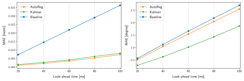
Figure 9. Position error (left) and angular error (right) in terms of MAE. Averages over 14 traces are shown.

Statistical significance

To verify that the gain obtained by the Kalman filter over Baseline is statistically significant, we applied a two-sample T-test on the angular errors obtained by the Baseline and Kalman filter, for each trace and LAT combination. Consequently, we reject the null hypothesis $\mathrm{H}_{0}$ of identical means of the angular error of the Baseline model and the Kalman filter-based prediction with $p<0.05$.

5.5. Limitations

During the trace recordings, we observed that the HoloLens flips the sign of a quaternion, when its real (scalar) component $q_{w}$ approaches $\pm 0.5$. Since a quaternion $\mathbf{q}$ and its negative $\mathbf{-q}$ correspond to the same orientation on the unit sphere (Solà, 2017), this behavior does not lead to a discontinuity in the rotation space. However, the Kalman filter assumes that all latent and observed variables have a Gaussian distribution which cannot model the true topology of the spherical quantities (Kurz et al., 2016a). Therefore, these ”jumps” in our data are detrimental to the performance of our predictor and cause large peak errors.

As a workaround, we compare a new measurement $\mathbf{z}_{k}$ with the previous one $\mathbf{z}_{k-1}$ at each iteration of the filter and reset the filter by re-initializing the state $\mathbf{x}$ and error covariance $\mathrm{\mathbf{P}}$, whenever a sign flip is detected. This workaround partially alleviates the peak errors observed after quaternion sign flips. However, the filter requires a few iterations to output good predictions again which causes a few large outliers after a re-initialization. In Sec. 6, we identify some techniques that correctly handle spherical distributions and thus may reduce the observed peak errors.

6. Conclusions and Future work

This paper presented a Kalman filter-based framework for prediction of head motion in order to reduce the interaction (motion-to-photon) latency of a cloud-based volumetric streaming system. We evaluated our approach using real head motion traces for different look-ahead times. Our results show that the proposed approach can predict head orientation $0.30.9\text{\,}\mathrm{d}\mathrm{e}\mathrm{g}$ more accurately than the benchmark AutoReg model for a tested range of LATs $20100\text{\,}\mathrm{m}\mathrm{s}$. Moreover, once its parameters are tuned, the Kalman filter is more robust to variations in data compared to the AutoReg model that has varying performance depending on the training data and needs training to learn its model coefficients.

However, the presented approach exhibits several shortcomings that can be addressed in future research. Particularly, our approach can be improved in terms of predicting spherical quantities. In our future work, we will use recursive filters based on spherical distributions such as von-Mises-Fisher (Kurz et al., 2016b) and Bingham distribution (Kurz et al., 2016b) to predict head orientations more accurately. These techniques rely on circular statistics and correctly handle the estimation in which the state is represented by a point on the unit sphere (Kurz et al., 2016a).

Another promising direction is to take into account the content properties of the volumetric video (in addition to sensor measurements). Such content-based techniques that take into account the visual saliency have recently been successfully applied for viewport prediction in 360-degree videos (Aladagli et al., 2017; Nguyen et al., 2018; Ozcinar et al., 2019). We expect that extending these techniques to 6DoF volumetric videos can significantly improve the prediction accuracy.

Another open research area is the subjective evaluation of volumetric videos in AR/MR environments. Our evaluation of prediction accuracy was performed using the objective metrics position error and angular error. However, although these metrics give a good idea about the relative performance of different predictors, the effect on user experience in a real system cannot directly be inferred from our results. Moreover, AR/MR headsets like Microsoft HoloLens use post-rendering updates known as late-stage reprojection  (Microsoft, 2016) or time-warping (Van Waveren, 2016) to account for any slight head movement since the last head pose prediction that may cause ”judder” effects, i.e. unstable overlaid virtual objects. Through image warping, such corrections can compensate for prediction errors in 6DoF motion (Mark et al., 1997). Therefore, subjective tests are required to understand the effect of prediction together with post-rendering correction on the user perception in an AR/MR environment. In this regard, we are currently investigating the effect of latency and mispredictions on the subjective experience of the viewers.

References

- (1)
- ano ([n.d.]) [n.d.]. Anoynmous for peer review.
- Akaike (1973) Htrotugu Akaike. 1973. Maximum likelihood identification of Gaussian autoregressive moving average models. Biometrika 60, 2 (1973), 255–265. https://doi.org/10.1093/biomet/60.2.255
- Aladagli et al. (2017) A Deniz Aladagli, Erhan Ekmekcioglu, Dmitri Jarnikov, and Ahmet Kondoz. 2017. Predicting head trajectories in 360 virtual reality videos. In 2017 International Conference on 3D Immersion (IC3D). IEEE, 1–6. https://doi.org/10.1109/IC3D.2017.8251913
- Azuma (1995) Ronald Azuma. 1995. Predictive tracking for augmented reality. Dissertation. University of North Carolina at Chapel Hill.
- Azuma and Bishop (1995) Ronald Azuma and Gary Bishop. 1995. A frequency-domain analysis of head-motion prediction. In Proceedings of the 22nd annual conference on Computer graphics and interactive techniques - SIGGRAPH ’95. ACM Press, 401–408. https://doi.org/10.1145/218380.218496
- Bao et al. (2016) Yanan Bao, Huasen Wu, Tianxiao Zhang, Albara Ah Ramli, and Xin Liu. 2016. Shooting a moving target: Motion-prediction-based transmission for 360-degree videos. In 2016 IEEE International Conference on Big Data (Big Data). IEEE, 1161–1170. https://doi.org/10.1109/bigdata.2016.7840720
- Bar-Shalom et al. (2004) Yaakov Bar-Shalom, X Rong Li, and Thiagalingam Kirubarajan. 2004. Estimation with applications to tracking and navigation: theory algorithms and software. John Wiley & Sons.
- Beigbeder et al. (2004) Tom Beigbeder, Rory Coughlan, Corey Lusher, John Plunkett, Emmanuel Agu, and Mark Claypool. 2004. The Effects of Loss and Latency on User Performance in Unreal Tournament 2003. In Proceedings of 3rd ACM SIGCOMM Workshop on Network and System Support for Games (NetGames ’04). ACM, 144–151. https://doi.org/10.1145/1016540.1016556
- Chartrand (2011) Rick Chartrand. 2011. Numerical differentiation of noisy, nonsmooth data. ISRN Applied Mathematics 2011 (2011). https://doi.org/10.5402/2011/164564
- Clemm et al. (2020) Alexander Clemm, Maria Torres Vega, Hemanth Kumar Ravuri, Tim Wauters, and Filip De Turck. 2020. Toward Truly Immersive Holographic-Type Communication: Challenges and Solutions. IEEE Communications Magazine 58, 1 (2020), 93–99.
- Cullen Jennings (2019) Jan-Ivar Bruaroey Cullen Jennings, Henrik Boström. 2019. WebRTC 1.0: Real-time Communication Between Browsers. https://www.w3.org/TR/webrtc/. Online (W3C specification); accessed: 2020-05-19.
- de la Fuente et al. (2019) Y. S. de la Fuente, G. S. Bhullar, R. Skupin, C. Hellge, and T. Schierl. 2019. Delay Impact on MPEG OMAF’s Tile-Based Viewport-Dependent 360 Video Streaming. IEEE Journal on Emerging and Selected Topics in Circuits and Systems 9, 1 (2019), 18–28. https://doi.org/10.1109/jetcas.2019.2899516
- Diebel (2006) James Diebel. 2006. Representing attitude: Euler angles, unit quaternions, and rotation vectors. Matrix 58, 15-16 (2006), 1–35.
- Eisert and Hilsmann (2020) Peter Eisert and Anna Hilsmann. 2020. Hybrid Human Modeling: Making Volumetric Video Animatable. In Real VR - Immersive Digital Reality: How to Import the Real World into Head-Mounted Immersive Displays, Marcus Magnor and Alexander Sorkine-Hornung (Eds.). Springer International Publishing, Cham, 167–187. https://doi.org/10.1007/978-3-030-41816-8_7
- Himberg and Motai (2009) Henry Himberg and Yuichi Motai. 2009. Head Orientation Prediction: Delta Quaternions Versus Quaternions. IEEE Transactions on Systems, Man, and Cybernetics, Part B (Cybernetics) 39, 6 (2009), 1382–1392. https://doi.org/10.1109/TSMCB.2009.2016571
- Hogg et al. (2005) Robert V Hogg, Joseph McKean, and Allen T Craig. 2005. Introduction to mathematical statistics. Pearson Education.
- Hosseini and Timmerer (2018) Mohammad Hosseini and Christian Timmerer. 2018. Dynamic Adaptive Point Cloud Streaming. In Proceedings of the 23rd Packet Video Workshop (PV ’18). ACM, New York, NY, USA, 25–30. https://doi.org/10.1145/3210424.3210429
- Hyndman and Athanasopoulos (2018) Rob J Hyndman and George Athanasopoulos. 2018. Forecasting: principles and practice. OTexts.
- Jia (2013) Yan-Bin Jia. 2013. Quaternions and Rotations. http://graphics.stanford.edu/courses/cs348a-17-winter/Papers/quaternion.pdf. Online; accessed: 2020-05-23.
- Kiruluta et al. (1997) Andrew Kiruluta, Moshe Eizenman, and Subbarayan Pasupathy. 1997. Predictive head movement tracking using a Kalman filter. IEEE Transactions on Systems, Man, and Cybernetics, Part B (Cybernetics) 27, 2 (1997), 326–331. https://doi.org/10.1109/3477.558841
- Kraft (2003) Edgar Kraft. 2003. A quaternion-based unscented Kalman filter for orientation tracking. In Sixth International Conference of Information Fusion, 2003. Proceedings of the, Vol. 1. IEEE, 47–54. https://doi.org/10.1109/ICIF.2003.177425
- Kurz et al. (2016a) Gerhard Kurz, Igor Gilitschenski, and Uwe D. Hanebeck. 2016a. Recursive Bayesian filtering in circular state spaces. IEEE Aerospace and Electronic Systems Magazine 31, 3 (2016), 70–87. https://doi.org/10.1109/MAES.2016.150083
- Kurz et al. (2016b) Gerhard Kurz, Igor Gilitschenski, and Uwe D Hanebeck. 2016b. Unscented von mises–fisher filtering. IEEE Signal Processing Letters 23, 4 (2016), 463–467.
- Labbe (2015) Roger Labbe. 2015. Kalman and Bayesian filters in Python. https://github.com/rlabbe/Kalman-and-Bayesian-Filters-in-Python. Online; accessed: 2020-05-14.
- LaViola (2003) Joseph J. LaViola. 2003. A comparison of unscented and extended Kalman filtering for estimating quaternion motion. In Proceedings of the 2003 American Control Conference, 2003., Vol. 3. 2435–2440 vol.3. https://doi.org/10.1109/ACC.2003.1243440
- Liu et al. (2018) Yang Liu, Haiwei Dong, Longyu Zhang, and Abdulmotaleb El Saddik. 2018. Technical Evaluation of HoloLens for Multimedia: A First Look. IEEE MultiMedia 25, 4 (2018), 8–18. https://doi.org/10.1109/MMUL.2018.2873473
- Livingston and Ai (2008) Mark A Livingston and Zhuming Ai. 2008. The effect of registration error on tracking distant augmented objects. In 2008 7th IEEE/ACM International Symposium on Mixed and Augmented Reality. IEEE, 77–86. https://doi.org/10.1109/ISMAR.2008.4637329
- Mangiante et al. (2017) Simone Mangiante, Guenter Klas, Amit Navon, Zhuang GuanHua, Ju Ran, and Marco Dias Silva. 2017. VR is on the edge: How to deliver 360 videos in mobile networks. In Proceedings of the Workshop on Virtual Reality and Augmented Reality Network. ACM, 30–35. https://doi.org/10.1145/3097895.3097901
- Mark et al. (1997) William R Mark, Leonard McMillan, and Gary Bishop. 1997. Post-rendering 3D warping. In Proceedings of the 1997 symposium on Interactive 3D graphics. 7–ff. https://doi.org/10.1145/253284.253292
- McCandless et al. (2000) Jeffrey W. McCandless, Stephen R. Ellis, and Bernard D. Adelstein. 2000. Localization of a Time-Delayed, Monocular Virtual Object Superimposed on a Real Environment. Presence: Teleoperators and Virtual Environments 9, 1 (2000), 15–24. https://doi.org/10.1162/105474600566583
- Microsoft (2016) Microsoft. 2016. Hologram stabilization. https://microsoft.github.io/MixedRealityToolkit-Unity/Documentation/hologram-stabilization.html. Online; accessed: 2020-05-24.
- Nguyen et al. (2018) Anh Nguyen, Zhisheng Yan, and Klara Nahrstedt. 2018. Your attention is unique: Detecting 360-degree video saliency in head-mounted display for head movement prediction. In Proceedings of the 26th ACM international conference on Multimedia. 1190–1198. https://doi.org/10.1145/3240508.3240669
- NVIDIA (2019) NVIDIA. 2019. NVIDIA CloudXR Delivers Low-Latency AR/VR Streaming Over 5G Networks to Any Device. https://blogs.nvidia.com/blog/2019/10/22/nvidia-cloudxr. Online; accessed: 2020-03-26.
- Ozcinar et al. (2019) Cagri Ozcinar, Julian Cabrera, and Aljosa Smolic. 2019. Visual Attention-Aware Omnidirectional Video Streaming Using Optimal Tiles for Virtual Reality. IEEE Journal on Emerging and Selected Topics in Circuits and Systems 9, 1 (2019), 217–230. https://doi.org/10.1109/jetcas.2019.2895096
- Park et al. (2019) Jounsup Park, Philip A Chou, and Jenq-Neng Hwang. 2019. Rate-utility optimized streaming of volumetric media for augmented reality. IEEE Journal on Emerging and Selected Topics in Circuits and Systems 9, 1 (2019), 149–162. https://doi.org/10.1109/jetcas.2019.2898622
- Petrangeli et al. (2019) Stefano Petrangeli, Gwendal Simon, Haoliang Wang, and Vishy Swaminathan. 2019. Dynamic Adaptive Streaming for Augmented Reality Applications. In 2019 IEEE International Symposium on Multimedia (ISM). IEEE, 56–567. https://doi.org/10.1109/ism46123.2019.00017
- Qian et al. (2019) Feng Qian, Bo Han, Jarrell Pair, and Vijay Gopalakrishnan. 2019. Toward practical volumetric video streaming on commodity smartphones. In Proceedings of the 20th International Workshop on Mobile Computing Systems and Applications. ACM, 135–140. https://doi.org/10.1145/3301293.3302358
- Qian et al. (2018) Feng Qian, Bo Han, Qingyang Xiao, and Vijay Gopalakrishnan. 2018. Flare: Practical Viewport-Adaptive 360-Degree Video Streaming for Mobile Devices. In Proceedings of the 24th Annual International Conference on Mobile Computing and Networking (MobiCom ’18). ACM, New York, NY, USA, 99–114. https://doi.org/10.1145/3241539.3241565
- Rossignac (1999) Jarek Rossignac. 1999. Edgebreaker: Connectivity compression for triangle meshes. IEEE transactions on visualization and computer graphics 5, 1 (1999), 47–61. https://doi.org/10.1109/2945.764870
- Savitzky and Golay (1964) Abraham Savitzky and Marcel JE Golay. 1964. Smoothing and differentiation of data by simplified least squares procedures. Analytical chemistry 36, 8 (1964), 1627–1639. https://doi.org/10.1021/ac60214a047
- Schreer et al. (2019a) O Schreer, I Feldmann, P Kauff, P Eisert, D Tatzelt, C Hellge, K Müller, T Ebner, and S Bliedung. 2019a. Lessons learnt during one year of commercial volumetric video production. In 2019 IBC conference. IBC.
- Schreer et al. (2019b) Oliver Schreer, Ingo Feldmann, Sylvain Renault, Marcus Zepp, Markus Worchel, Peter Eisert, and Peter Kauff. 2019b. Capture and 3D video processing of volumetric video. In 2019 IEEE International Conference on Image Processing (ICIP). IEEE, 4310–4314. https://doi.org/10.1109/icip.2019.8803576
- Schwarz et al. (2019) Sebastian Schwarz, Marius Preda, Vittorio Baroncini, Madhukar Budagavi, Pablo Cesar, Philip A. Chou, Robert A. Cohen, Maja Krivokuća, Sebastien Lasserre, Zhu Li, Joan Llach, Khaled Mammou, Rufael Mekuria, Ohji Nakagami, Ernestasia Siahaan, Ali Tabatabai, Alexis M. Tourapis, and Vladyslav Zakharchenko. 2019. Emerging MPEG Standards for Point Cloud Compression. IEEE Journal on Emerging and Selected Topics in Circuits and Systems 9, 1 (2019), 133–148. https://doi.org/10.1109/JETCAS.2018.2885981
- Seabold and Perktold (2010) Skipper Seabold and Josef Perktold. 2010. statsmodels: Econometric and statistical modeling with python. In 9th Python in Science Conference. inproceedings.
- Shi et al. (2019) Shu Shi, Varun Gupta, Michael Hwang, and Rittwik Jana. 2019. Mobile VR on edge cloud: a latency-driven design. In Proceedings of the 10th ACM Multimedia Systems Conference. ACM, 222–231. https://doi.org/10.1145/3304109.3306217
- Shi and Hsu (2015) Shu Shi and Cheng-Hsin Hsu. 2015. A survey of interactive remote rendering systems. Comput. Surveys 47, 4 (May 2015), 1–29. https://doi.org/10.1145/2719921
- Shi et al. (2012) Shu Shi, Klara Nahrstedt, and Roy Campbell. 2012. A real-time remote rendering system for interactive mobile graphics. ACM Transactions on Multimedia Computing, Communications, and Applications (TOMM) 8, 3s (2012), 1–20. https://doi.org/10.1145/2348816.2348825
- Shoemake (1985) Ken Shoemake. 1985. Animating rotation with quaternion curves. In ACM SIGGRAPH computer graphics, Vol. 19. ACM, 245–254. https://doi.org/10.1145/325165.325242
- Solà (2017) Joan Solà. 2017. Quaternion kinematics for the error-state Kalman filter. CoRR abs/1711.02508 (2017). arXiv:1711.02508 http://arxiv.org/abs/1711.02508
- van der Hooft et al. (2019) Jeroen van der Hooft, Tim Wauters, Filip De Turck, Christian Timmerer, and Hermann Hellwagner. 2019. Towards 6DoF HTTP adaptive streaming through point cloud compression. In Proceedings of the 27th ACM International Conference on Multimedia. 2405–2413. https://doi.org/10.1145/3343031.3350917
- van Rhijn et al. (2005) A. van Rhijn, R. van Liere, and J.D. Mulder. 2005. An analysis of orientation prediction and filtering methods for VR/AR. In IEEE Proceedings. VR 2005. Virtual Reality, 2005. IEEE, 67–74. https://doi.org/10.1109/VR.2005.1492755
- Van Waveren (2016) JMP Van Waveren. 2016. The asynchronous time warp for virtual reality on consumer hardware. In Proceedings of the 22nd ACM Conference on Virtual Reality Software and Technology. ACM, 37–46. https://doi.org/10.1145/2993369.2993375
- Welch and Bishop (1995) Greg Welch and Gary Bishop. 1995. An introduction to the Kalman filter. Technical Report TR 95-041. University of North Carolina.