We obtain turnpike results for optimal control problems with lack of stabilizability in the state equation and/or detectability in the state term in the cost functional.
We show how, under weakened stabilizability/detectability conditions, terminal conditions may affect turnpike phenomena.
Numerical simulations have been performed to illustrate the theoretical results.
(Noboru Sakamoto) Supported, in part, by JSPS KAK-
ENHI Grant Number JP19K04446 and by Nanzan University Pache Research Subsidy I-A-2 for 2019 academic year.
(Dario Pighin)
This project has received funding from the European Research Council (ERC) under the European Union’s Horizon 2020 research and innovation programme (grant agreement NO. 694126-DyCon).
Dario Pighin
Departamento de Matemáticas, Universidad Autónoma de Madrid
28049 Madrid, Spain
Chair of Computational Mathematics, Fundación Deusto
University of Deusto, 48007, Bilbao, Basque Country, Spain
Noboru Sakamoto
Faculty of Science and Engineering, Nanzan University
Yamazato-cho 18, Showa-ku, Nagoya, 464-8673, Japan
Introduction
The purpose of this manuscript is to check the validity of the turnpike property for linear quadratic optimal control problems, with weak observation of the state in the cost functional. We consider the time-evolution optimal control problem
where:
and the corresponding steady one
The time-evolution problem satisfies the turnpike property if the time-evolution optimal pair approximate the steady optimal pair as the time horizon .
Typically, for turnpike to hold, the pair is required to be stabilizable and the pair is asked to be detectable (see, e.g. [21, 32, 28]). Our goal is to check if turnpike holds for the full control and the detected state, under weakened detectability and controllability assumptions.
The study of the behaviour of control problems in long time and the turnpike property is a classical topic in the literature. We provide just some essential references. A pioneer on the topic has been the econometrician Paul Samuelson (see [9, 29, 18]). Later on the topic has been studied both in Mathematics and in Economic Sciences [19, 36, 26, 14, 2, 23, 24, 10]. The infinite dimensional case has been explored [1, 7, 8]. An extensive review on the topic is [37]. More recently, the topic has been studied in [21, 32, 22, 31, 30, 13, 12, 20]. Related results have been obtained in Mean Field Games (see, for instance, [5, 6]).
We distinguish two cases:
•
section 1: free endpoint (the state left free at final time );
•
section 2: fixed endpoint (the state has to match a given final target at time ).
In section 1, we suppose the state is left free at . We can then employ Kalman decomposition (see, e.g. [38, section 3.3]) to decompose the state space into a detectable part and an undetectable one. In Proposition 1, we prove that an exponential turnpike property is satisfied by the full control and the detected state if and only if the observable modes are stabilizable. In particular, if the state equation is stabilizable, the turnpike property holds for the full control and the detected state, without any observability assumptions on the cost functional (Corollary 1).
These results rely on the absence of final condition for the state. As a consequence of that, unobservable modes do not influence the value of the cost functional, i.e. they are irrelevant for the sake of optimization.
In subsections 1.2 and 1.3, the above results are employed in the context of pointwise control of respectively the heat and wave equation. We project the state equation onto a finite number of Fourier modes. For the heat equation with potential, the full control and the observed state fulfils turnpike if and only if whenever an eigenfunction is non-zero on the observation point, either the same eigenfunction is non-zero on the control point or the point is stable for the free dynamics. For the wave equation, a more restricted condition is required. The turnpike property is verified by the full control and the observed state if and only if whenever an eigenfunction vanishes on the control point, it vanishes on the observation point as well.
In section 2, we deal with a fixed endpoint problem. Therefore,
•
on the one hand, in the running cost we penalize only the observed state;
•
on the other hand, the unobservable modes are relevant to fulfill the final condition. Namely, the unobservable component of the system enters in the definition of the set of admissible controls, where the functional is minimized.
For this reason, we need to assume controllability of the full state equation and we cannot employ Kalman decomposition to get rid of the unobservable component. In Proposition 4, we prove that the turnpike property is verified for full control and state, if the unobservable modes of are not critical (they are not associated to a purely imaginary eigenvalue of the free dynamics). In particular, turnpike can hold even if both stable and unstable modes of are not observable. This condition is formulated as weak Hautus test.
Inspired by [10], we study a class of optimal control problems with fixed endpoint, where the Hamiltonian matrix may have imaginary eigenvalues. In Proposition 5 we prove that basically the exponential turnpike is satisfied by the control and the observed state, while the unobserved state is linear in time, up to an exponentially small remainder. We show how this result applies to the illustrative example in [10, section 3].
1. Free endpoint problem
1.1. Statement of the main results
We consider the linear quadratic optimal control problem:
(1)
where:
(2)
The matrix describes the free dynamics, while the action of the control is defined by multiplication by the matrix . is an observation matrix. By the Direct Methods in the Calculus of Variations and strict convexity, the above problem admits a unique optimal control denoted by . The optimal state is denoted by . Furthermore, by strict convexity, the optimal control is the unique solution to the optimality system
(3)
The corresponding steady problem reads as
(4)
The well posedeness of the steady problem follows from the following Lemma.
Lemma 1.1.
Let , , and . Set
and
(5)
Then,
(1)
there exists global minimizer for over ;
(2)
the set of global minimizers of is given by
We prove this Lemma in the Appendix.
Inspired by [3, Definition 2.1, page 480], we give the following definition of -stabilizability, namely stabilizability of the observable part of the state.
Definition 1.2.
Let , and . is said to be -stabilizable if there exists a feedback matrix , such that
for some , .
We introduce the concept of -turnpike, i.e. turnpike for the full control and the detected state. To this end, let us decompose the state space into a detectable part and an undetectable one. We start be defining some observability and detectability concepts. Let be a time horizon. The output operator is defined as
(6)
for any . The subspace is called the unobservable space, which admits an algebraic representation [33, Propositon 1.4.7]
(7)
We define the observable space as the orthogonal . The undetectbale space is defined as the subspace , made of those unobservable modes which are not stable. By (7),
The detectable space is defined as .
We are now in position to decompose the state space into a detectable part and an undetectable one
where
and
The matrix associated to the orthogonal projection onto is denoted by , while the matrix associated to the projection onto is indicated by . For any ,
(8)
If is detectable, is the identity matrix.
Definition 1.3.
Let , and . Let be the corresponding projection onto the detectable space , as in (8). The triplet enjoys -turnpike if, for any initial datum and target , there exists and , such that, for any ,
where is the optimal pair for (2)-(1) and is a minimizer for the steady functional (5).
As we announced, the main assumption of the following Proposition is that observable modes are stabilizable.
Proposition 1.
In the above notation, the triplet enjoys -turnpike if and only if is -stabilizable.
is stabilizable. Then, for any , is -stabilizable. Hence, Proposition 1 yields the conclusion.
∎
In subsection 1.2 we apply our theory to the pointwise control of the heat equation and in subsection 1.3 we illustrate how our theory works in the pointwise control of the wave equation. In subsection 1.4, we prove Proposition 1.
1.2. Pointwise control of the heat equation
Let be a connected bounded open set of , , with boundary. Inspired by [17, section 1.2], we consider a heat equation controlled from one point
(9)
where is the state, while is the control and is the Dirac delta at , i.e. the control acts on . The potential coefficient is supposed to be bounded. Following [17, subsection 1.2.2], one can prove that for any and , there exists a unique solution by transposition to (9), with initial datum and control .
We derive now a finite-dimensional Fourier approximation of the above controlled equation. We assume that the spectrum of is simple. Let be the spectrum of and let be a corresponding set of eigenfunctions, orthonormal basis of .
Fix . The projection of (9) on the finite dimensional space reads as
(10)
where is an diagonal matrix
(11)
the control operator is an matrix
(12)
and the initial datum
We consider the optimal control problem:
(13)
where is the state solution to (10), with control and initial datum , the scalar is a running target and
namely the state is observed on .
Proposition 2.
The triplet enjoys -turnpike if and only if for any such that , either or .
Hence, since the spectrum of the Dirichlet laplacian is simple, the observable subspace is
and the stabilizable subspace reads as
Then, if and only if
Then, by Proposition 1, the triplet enjoys -turnpike if and only if for any such that , either or .
∎
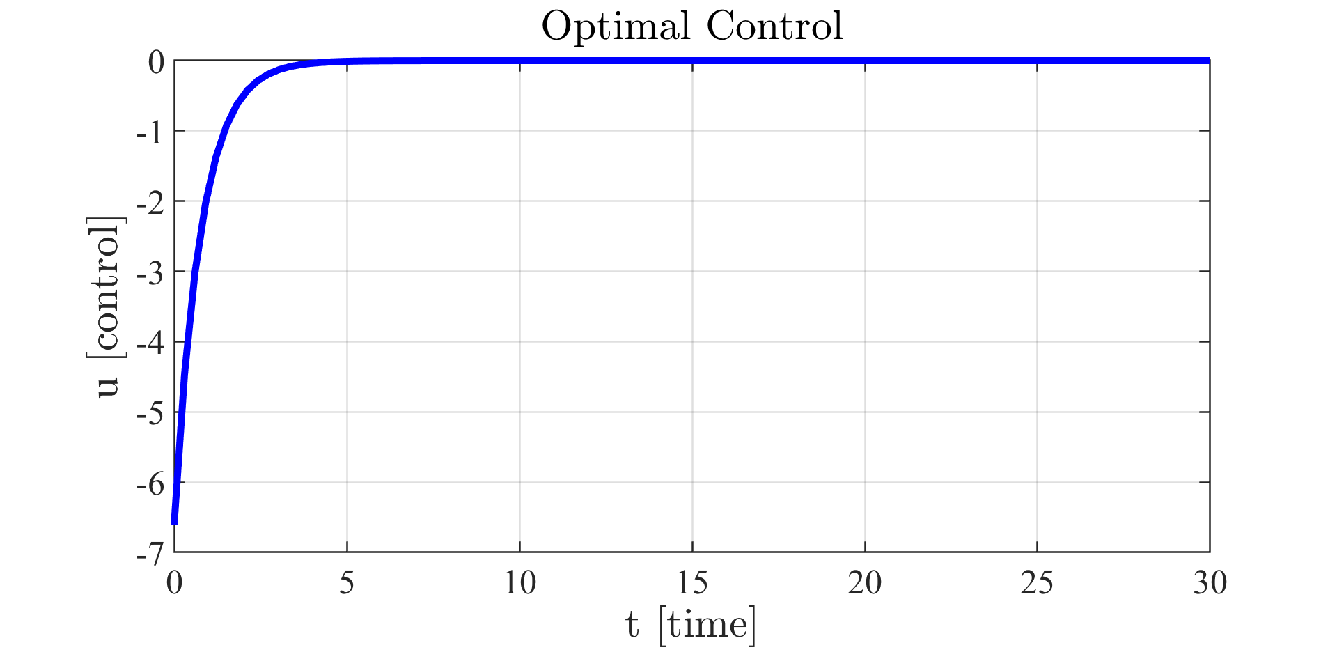
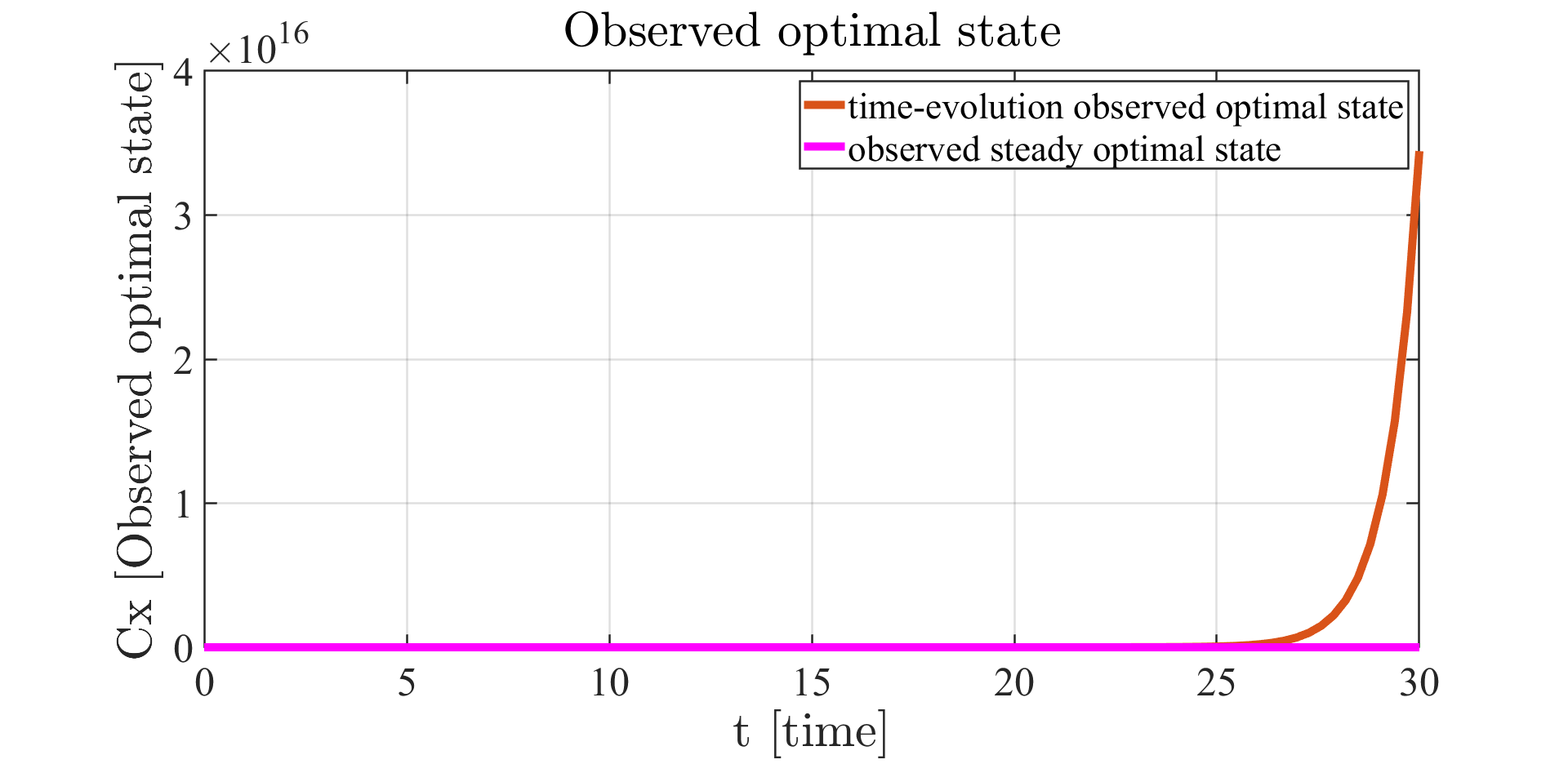
We have performed some numerical simulations employing a conjugate gradient method (see [25, algorithm 2 page 111]). In our notation, we chose domain , , potential coefficient , , , target and initial datum . The results are depicted in figures 1 and 2.
Figure 1. Optimal control for (13) subject to (10), with , , , , , target and initial datum .Figure 2. Observed optimal state for (13) subject to (10), with , , , , , target and initial datum .
1.3. Pointwise control of the wave equation
Let be a connected bounded open set of , , with boundary.
As in [17, section 1.3], we consider the wave equation controlled from
(15)
where is the state, while is the control whose action is localized on the point by means of multiplication with the Dirac delta . The well posedeness of the above equation was analyzed in [17, subsection 1.3.2], by using transposition techniques. For any , and , there exists a unique solution by transposition to (15), with initial datum and control .
We suppose that the spectrum of the Dirichlet laplacian is simple. Let be an orthonormal basis of , such that .
Fix . Set
(16)
The projection of (15) onto the finite dimensional space reads as
(17)
where is an matrix
(18)
the control operator is an matrix
(19)
and the initial datum
We consider the optimal control problem:
(20)
where is the state solution to (17), with control and initial datum , the scalar is a running target and
namely the state is observed on .
We have the following result.
Proposition 3.
The triplet enjoys -turnpike if and only if for any such that , we have .
As in the proof of Proposition 2, we define the observable subspace
(21)
and the stabilizable subspace
where in this case and are given respectively by (18) and (19).
The -stabilizability of is equivalent to the inclusion
On the one hand, for any natural , we have
and
On the other hand, for any natural , we have
and
Hence, since the spectrum of the Dirichlet laplacian is simple, the observable subspace is
and the stabilizable subspace reads as
Then, the inclusion holds if and only if
Then, by Proposition 1, the triplet enjoys -turnpike if and only if for any such that , .
∎
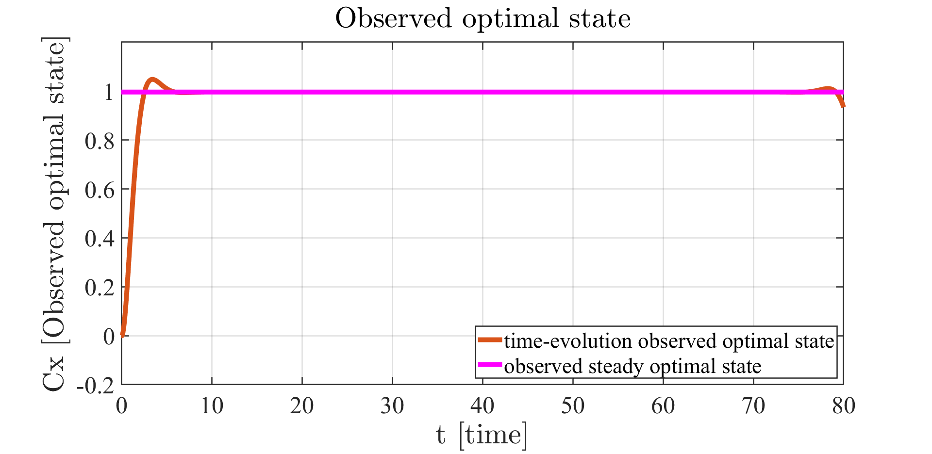
We carried out some numerical simulations using the interior-point optimization routine IPOpt (see [34] and [35]) coupled with AMPL [11], which serves as modelling language and performs the automatic differentiation. In our notation, we chose domain , , , , target and initial datum . The results are illustrated in figures 3 and 4.
Figure 3. Optimal control for (17)-(20), with , , , , and .Figure 4. Observed optimal state for (17)-(20), with , , , , and .
The key-tool for our analysis of the control problem (2)-(1) is the Kalman decomposition (see, e.g. [38, section 3.3]). In the notation of [4], denote the -invariant subspace of spanned by the generalized eigenvectors of corresponding to eigenvalues of such that . We decompose the state space into an detectable part and an undetectable one
where
(22)
and
(23)
The matrix associated to the orthogonal projection onto is denoted by , while the matrix associated to the projection onto is indicated by . Hence, for any ,
In the notation of [4], denote the -invariant subspace of spanned by the generalized eigenvectors of corresponding to eigenvalues of such that and the stabilizable subspace
An essential tool for the proof of Proposition 1 is the following Lemma.
Lemma 1.4.
Let , and . is -stabilizable if and only if for any initial datum , there exists a control , such that
(26)
being the solution to (2), with initial datum and control .
The above Lemma follows from [3, Remark 2.2 page 24] applied to the detectable space , introduced in (23).
Step 1Necessity of the -stabilizability of
Suppose enjoys -turnpike. Then, taking target , for any initial datum , we have
being the optimal pair for (2)-(1), with target and initial datum , whence
(27)
where is independent of the time horizon . By Banach-Alaoglu Theorem, there exists , such that, up to subsequences,
weakly in . We denote by the solution to (2), with initial datum and control . Arbitrarily fix . By definition of weak convergence, up to subsequences
weakly in . By lower-semicontinuity of the norm with respect to the weak convergence and (27), for any , we have
whence, by the arbitrariness of ,
Then, by Lemma 1.4, is -stabilizable.
Step 2We rewrite the functional employing Kalman decomposition
Assume is -stabilizable. Take any initial datum and control . Let be the corresponding solution to the state equation
Then, the functional introduced in (2)-(1) can be rewritten as
(30)
where:
(31)
Step 3Sufficiency of -stabilizability of
Let be the optimal control and be the optimal state for the optimal control problem (31)-(30).
By construction, is detectable on and, since is -stabilizable,
is stabilizable on . Then, by [28, Corollary 3.2] applied to (31)-(30), we have
and being independent of the time horizon. Then, the triplet enjoys -turnpike, as desired.
∎
2. Fixed endpoint problem
In this section, we consider an optimal control problem for (2) with arbitrarily prescribed terminal state. Let an initial datum and a final target be given.
In the notation of section 1, assume is controllable. Consider the control system
(32)
We introduce the set of admissible controls
(33)
We consider the linear quadratic optimal control problem:
(34)
where is a running target. By the Direct Methods in the Calculus of Variations and strict convexity, the above problem admits a unique optimal control denoted by . The optimal state is denoted by . Furthermore, by strict convexity, the optimal control , where is the unique solution to the optimality system
(35)
As in the free endpoint problem, the steady problem is a minimization problem in finite dimension under linear constraints
The corresponding steady problem reads as
As we anticipated, the fixed endpoint case is more delicate. Indeed,
•
in the functional, we penalize only the observable part of the state;
•
in the definition of the set of admissible control, we impose a final condition , which involves the full state, including the unobservable part.
We cannot expect the classical turnpike property to be valid, without any additional assumptions on . Indeed, take skew adjoint and . The resulting optimal control is oscillatory, thus violating the turnpike property.
The turnpike property is verified by the full state and adjoint state if fulfills the weak Hautus test, introduced in definition (2.1) below. In subsection 2.2, inspired by [10], we study velocity turnpike in case the Hamiltonian matrix has imaginary eigenvalues.
2.1. The sufficiency of the weak Hautus test for exponential turnpike
Definition 2.1.
Take as in (32)-(34). The pair is said to satisfy the weak Hautus test if
(37)
where denotes the spectrum of , stands for the imaginary unit and .
Note that the difference with respect to the classical Hautus test (see, e.g. [33, Proposition 1.5.1]) is that the above rank condition has to be checked only for purely imaginary eigenvalues . Namely, only eigenvectors of imaginary eigenvalues of are required to be observable.
Proposition 4.
Suppose is controllable and the weak Hautus test (37) is satisfied. Take . Let be an optimal control for (32)-(34) and be the optimal state. There exist -independent and such that
(38)
where is the unique solution to the steady problem (36).
The proof of the sufficiency of the weak Hautus test (37) (available at the end of the present section) is based on Lemma 2.2, Lemma 2.3 and Lemma 2.4, concerning the properties of the optimality system (35) and its associated matrix, the so-called Hamiltonian matrix
(39)
Lemma 2.2 is well-known in the literature (see e.g. [15, Lemma 8]). However, we provide the proof for the reader’s convenience.
Lemma 2.2.
Consider the Hamiltonian matrix Ham introduced in (39). Assume is stabilizable. We have if and only if the weak Hautus test is satisfied.
Since is stabilizable, the Algebraic Riccati Equation
(40)
admits a unique antistrong solution , a symmetric and positive semidefinite matrix, such that has all eigenvalues with nonpositive real parts (see e.g. [16] and references therein). As in [27] and [16, formula (3.8) page 57], set
This, together with [4, Fact 1-(f)], yields the equivalence between and , with
To conclude, we have to prove that if and only if satisfies the weak Hautus test (37). On the one hand, if , then for any eigenvector corresponding to imaginary eigenvalue of and for any
(41)
Since , we have , whence
as required. On the other hand, suppose (37) is verified. Suppose, by contradiction, that . Since is -invariant,
there exists a nonzero eigenvector corresponding to an imaginary eigenvalue . By (41), this leads to , which yields
so obtaining a contradiction, as desired.
∎
We now provide a global bound of the norm of the adjoint state, uniform in the time horizon .
Lemma 2.3.
Consider the control problem (32)-(34). There exists such that, for any time horizon and time instant , we have
Step 1Reduction to the case running target
By Lemma B.1, the vector , whence there exists solving the steady optimality system
(43)
Introduce the perturbation variables and . We realize that the pair solves
(44)
the optimality system for the control problem (32)-(34), with terminal conditions and . This allows us to reduce to the case . To avoid weighting the notation, we will drop the tilde in and .
Step 2Upper bound for the minimum value of the functional
Consider the control
(45)
where
drives the control system (32) from to in time and steers (32) from to in time . Consequently the control , steers the system from to in time .
Now, for , the control operates in an interval of length one. Then, there exists some , independent of , such that
whence
(46)
Now, let be the solution to (32), with control . By definition of , , for , whence
(47)
the constant being independent of the time horizon. Therefore, by (46) and (47) and since is a minimizer of ,
(48)
Step 3Boundedness of and
By assumptions, is controllable. Then, is observable. Therefore, by adapting the techniques of [21, remark 2.1 page 4245], for every , we have
(49)
with independent of , as desired.
∎
Let be a square matrix. Following the notation of [4], , and denote resp. the -invariant subspaces of spanned by the generalized eigenvectors of corresponding to eigenvalues of such that , and . In the proof Proposition 4 we use the following Lemma, proved in the appendix.
Lemma 2.4.
Let be a square matrix. Let be a solution to
(50)
Then, for every
(51)
the constants and being independent of the time horizon.
Step 1Hyperbolicity of the Hamiltonian matrix
If the weak Hautus test (37) is verified, by Lemma 2.2, the critical subspace .
Step 2Uniqueness of the minimizer for the steady problem
By the above step, we have . Then, the steady optimality system
(52)
admits a unique solution , whence the optimal pair for the minimization problem (36) is unique and is given by .
Step 3Conclusion
If the weak Hautus test (37) is verified, by Lemma 2.2, the critical subspace . Then, Lemma 2.3 and Lemma 2.4 allow us to conclude.
∎
2.2. Exponential velocity turnpike
This subsection has been inspired by [10] where the notion of velocity turnpike has been introduced. In particular, we give a theoretical explanation of the illustrative example in [10, section 3]. Note that, in the proposition below the Hamiltonian matrix may have imaginary eigenvalues.
The optimal control for the time-evolution problem (32)-(34) reads as , where
(58)
By working in perturbation variables, as in the step 1 of the proof of Lemma 2.3, we can reduce to the case .
Step 1Change of variable
Set the linear transformation
(59)
By using the Algebraic Riccati Equation (40), we have222
Set further . Then the pair solves
(60)
Step 2Proof of the equality
By [4, fact 1.(f)-(d)] and the hypothesis , we have
as desired.
Step 5Proof of (57)
On the one hand, defining a control as in (45), we have the upper bound
(81)
On the other hand, employing (55) we get the lower bound
(82)
where the constant is independent of the time horizon and the terminal data and . Since ,
(81) together with (82) yields (57). This finishes the proof.
∎
Example 1.
We show now how our techniques apply in the example presented in [10, section 3]. We consider the control system
(83)
We introduce the set of admissible controls
(84)
We formulate the optimal control problem
(85)
For this special problem, we have , whence Proposition 5 is applicable.
We write the Algebraic Riccati Equation associated to the above problem
(86)
The unique positive semidefinite solution to the above equation is given by
(87)
whence
(88)
with spectrum . We have
•
;
•
;
•
;
•
.
We decompose
(89)
with the corresponding projections and .
By Proposition 5, there exist -independent and such that
Step 1Existence of minimizer
We introduce the equivalence relation in
We denote by the equivalence class of . Actually, , provided that . Then, we are in position to define
Now, by definition of and , for any the sublevel set
is compact. Hence, by the Weierstrass extreme value theorem, there exists global minimizer for . Then, is a global minimizer of .
Step 2Conclusion
By definition of and ,
Let us now prove the other inclusion by contradiction. Suppose there exists global minimizer such that
Then, either or
In both cases . Indeed, in the first case, from , we have . In the second case . Therefore, . Then, , whence . Now, the function
is strictly convex.
Then, . Hence is not a minimizer, so obtaining a contradiction. This finishes the proof.
∎
Appendix B Kernel and range of the Hamiltonian matrix
Let , and . We determine the kernel and the range of the Hamiltonian matrix
(93)
The above is the coefficient matrix of the optimality system (52) for the steady problem (4).
Step 1Stable, antistable and critical splitting
We have
where stands for the direct sum. Then, let be a solution to (50). Denote by , and resp. the projections of onto , and . Then, and, for ,
Step 2Estimate for the stable part
We have
All the eigenvalues of have strictly negative real part, where we have denoted by the linear operator associated to the matrix . Then,
we have, for any
(106)
the constant depending only on .
Step 3Estimate for the unstable part
By definition
(107)
Then, solves
(108)
Now, all the eigenvalues of have strictly negative real part. Then, as in Step 1,
[1]G. Allaire, A. Münch, and F. Periago, Long time behavior of a
two-phase optimal design for the heat equation, SIAM Journal on Control and
Optimization, 48 (2010), pp. 5333–5356.
[2]B. D. Anderson and P. V. Kokotovic, Optimal control problems over
large time intervals, Automatica, 23 (1987), pp. 355–363.
[3]A. Bensoussan, G. Da Prato, M. Delfour, and S. Mitter, Representation and Control of Infinite Dimensional Systems, Systems &
Control: Foundations & Applications, Birkhäuser Boston, 2006.
[4]F. M. Callier and J. Winkin, Convergence of the time-invariant
riccati differential equation towards its strong solution for stabilizable
systems, Journal of mathematical analysis and applications, 192 (1995),
pp. 230–257.
[5]P. Cardaliaguet, J.-M. Lasry, P.-L. Lions, and A. Porretta, Long
time average of mean field games., Networks & Heterogeneous Media, 7
(2012).
[6]P. Cardaliaguet, J.-M. Lasry, P.-L. Lions, and A. Porretta, Long
time average of mean field games with a nonlocal coupling, SIAM Journal on
Control and Optimization, 51 (2013), pp. 3558–3591.
[7]D. Carlson, A. Haurie, and A. Leizarowitz, Infinite Horizon Optimal
Control: Deterministic and Stochastic Systems, Springer Berlin Heidelberg,
2012.
[8]T. Damm, L. Grüne, M. Stieler, and K. Worthmann, An exponential
turnpike theorem for dissipative discrete time optimal control problems,
SIAM Journal on Control and Optimization, 52 (2014), pp. 1935–1957.
[9]R. Dorfman, P. Samuelson, and R. Solow, Linear Programming and
Economic Analysis, Dover Books on Advanced Mathematics, Dover Publications,
1958.
[10]T. Faulwasser, K. Flaßamp, S. Ober-Blöbaum, and K. Worthmann,
Towards velocity turnpikes in optimal control of mechanical systems,
IFAC-PapersOnLine, 52 (2019), pp. 490–495.
In Proc. 11th IFAC Symposium on Nonlinear Control Systems,
NOLCOS 2019.
[11]R. Fourer, D. M. Gay, and B. W. Kernighan, A modeling language for
mathematical programming, Management Science, 36 (1990), pp. 519–554.
[12]L. Grüne, M. Schaller, and A. Schiela, Sensitivity analysis of
optimal control for a class of parabolic pdes motivated by model predictive
control, SIAM Journal on Control and Optimization, 57 (2019),
pp. 2753–2774.
[13]L. Grüne, M. Schaller, and A. Schiela, Exponential sensitivity and
turnpike analysis for linear quadratic optimal control of general evolution
equations, Journal of Differential Equations, (2019).
[14]A. Haurie, Optimal control on an infinite time horizon: the turnpike
approach, Journal of Mathematical Economics, 3 (1976), pp. 81–102.
[15]V. Kucera, A contribution to matrix quadratic equations, IEEE
Transactions on Automatic Control, 17 (1972), pp. 344–347.
[16]V. Kučera, Algebraic riccati equation: Hermitian and definite
solutions, in The Riccati Equation, Springer, 1991, pp. 53–88.
[17]J. L. Lions, 1. Pointwise Control for Distributed Systems, 1992,
pp. 1–39.
[18]N. Liviatan and P. A. Samuelson, Notes on turnpikes: Stable and
unstable, Journal of Economic Theory, 1 (1969), pp. 454 – 475.
[19]L. W. McKenzie, Turnpike theorems for a generalized leontief model,
Econometrica: Journal of the Econometric Society, (1963), pp. 165–180.
[20]D. Pighin, The turnpike property in semilinear control, arXiv
preprint arXiv:2004.03269, (2020).
[21]A. Porretta and E. Zuazua, Long time versus steady state optimal
control, SIAM J. Control Optim., 51 (2013), pp. 4242–4273.
[22], Remarks on long time
versus steady state optimal control, in Mathematical Paradigms of Climate
Science, Springer, 2016, pp. 67–89.
[23]A. Rapaport and P. Cartigny, Turnpike theorems by a value function
approach, ESAIM: control, optimisation and calculus of variations, 10
(2004), pp. 123–141.
[24], Competition between
most rapid approach paths: necessary and sufficient conditions, Journal of
optimization theory and applications, 124 (2005), pp. 1–27.
[25]J.-P. Raymond, Optimal Control of Partial Differential Equations,
Université Paul Sabatier.
[26]R. Rockafellar, Saddle points of hamiltonian systems in convex
problems of lagrange, Journal of Optimization Theory and Applications, 12
(1973), pp. 367–390.
[27]W. E. Roth, On the matric equation x 2+ ax+ xb+ c= 0, Proceedings
of the American Mathematical Society, 1 (1950), pp. 586–589.
[28]N. Sakamoto, D. Pighin, and E. Zuazua, The turnpike property in
nonlinear optimal control — A geometric approach, in Proc. of 58th IEEE
Conference on Decision and Control, 2019, pp. 2422–2427.
[29]P. A. Samuelson, The general saddlepoint property of optimal-control
motions, Journal of Economic Theory, 5 (1972), pp. 102 – 120.
[30]E. Trélat and C. Zhang, Integral and measure-turnpike properties
for infinite-dimensional optimal control systems, Mathematics of Control,
Signals, and Systems, 30 (2018), p. 3.
[31]E. Trélat, C. Zhang, and E. Zuazua, Steady-state and periodic
exponential turnpike property for optimal control problems in hilbert
spaces, SIAM Journal on Control and Optimization, 56 (2018), pp. 1222–1252.
[32]E. Trélat and E. Zuazua, The turnpike property in
finite-dimensional nonlinear optimal control, Journal of Differential
Equations, 258 (2015), pp. 81–114.
[33]M. Tucsnak and G. Weiss, Observation and control for operator
semigroups, Springer Science & Business Media, 2009.
[34]A. Wächter and L. T. Biegler, On the implementation of an
interior-point filter line-search algorithm for large-scale nonlinear
programming, Mathematical programming, 106 (2006), pp. 25–57.
[35]A. Waechter, C. Laird, F. Margot, and Y. Kawajir, Introduction to
ipopt: A tutorial for downloading, installing, and using ipopt, Revision,
(2009).
[36]R. Wilde and P. Kokotovic, A dichotomy in linear control theory,
IEEE Transactions on Automatic control, 17 (1972), pp. 382–383.
[37]A. J. Zaslavski, Turnpike properties in the calculus of variations
and optimal control, vol. 80, Springer Science & Business Media, 2006.
[38]K. Zhou, J. Doyle, and K. Glover, Robust and Optimal Control,
Feher/Prentice Hall Digital and, Prentice Hall, 1996.