High-Order Phase Reduction for Coupled Oscillators

Abstract

We explore the phase reduction in networks of coupled oscillators in the higher orders of the coupling parameter. For coupled Stuart-Landau oscillators, where the phase can be introduced explicitly, we develop an analytic perturbation procedure to allow for the obtaining of the higher-order approximation explicitly. We demonstrate this by deriving the second-order phase equations for a network of three Stuart-Landau oscillators. For systems where explicit expressions of the phase are not available, we present a numerical procedure that constructs the phase dynamics equations for a small network of coupled units. We apply this approach to a network of three van der Pol oscillators and reveal components in the coupling with different scaling in the interaction strength.

1 Introduction

Networks of coupled self-sustained oscillators are widely used to describe complex rhythmical systems in physics [1, 2], biology [3, 4], and other fields [5, 6]. In particular, such models are relevant for the description of laser [7] and nanomechanical [8] oscillator arrays, coupled Josephson junctions [9] and spin-torque oscillators [10], power grids [11], the activity of neuronal populations [12], the interaction of different organs within a human body [13], cell assemblies [14], etc.

One of the most famous theoretical tools for the analysis of coupled oscillators is the phase reduction [15, 16, 17, 18]. This approach provides a recipe for a description of complex high-dimensional oscillators by a single cyclic variable, phase $\varphi$, so that the dynamics of a network of $N$ generally high-dimensional elements reduces to a set of $N$ coupled one-dimensional differential equations for the phases. This reduction is based on the slaving principle (the corresponding notion in mathematical literature is the normal hyperbolicity): While the phases correspond to the neutral directions with zero Lyapunov exponents, the “amplitudes” (i.e. all other variables except for the phases) are stable and thus follow the phase dynamics. As a result, the full system’s dynamics reduces to that on the $N$-dimensional torus spanned by the phases.

This reduction allows studying general behaviours of coupled oscillators through phase dynamics models, a prominent example here is the analytically tractable Kuramoto model of all-to-all interconnected units, derived for a population of weakly coupled oscillators close to the Hopf bifurcation point [19, 15, 20]. Generally, phase dynamics models are expected to be valid for arbitrary oscillators and weak to moderate coupling. However, the existing theory employs a perturbative approach and provides phase equations only in the first-order approximation in the coupling strength. Derivation of high-order corrections would extend the validity of the approach beyond the weak-coupling limit and, thus, essentially increase our ability to analyse complex networks. Yet, for the moment it remains a theoretical challenge, in spite of numerous attempts [21, 22, 23, 24, 25, 26].

In addition to obvious advantages for theoretical studies, phase reduction provides a framework for model reconstruction from measurements and, hence, plays an essential role in experimental research. Reconstruction of the phase dynamics equations from data is much more simple than recovery of equations for the state variables because (i) phase equations are low-dimensional and (ii) have a simple universal form because their right-hand sides are $2\pi$-periodic functions of the phases. Though precise estimation of the phases from scalar signals remains a topic of ongoing studies [27, 28, 29], phase models have been successfully recovered for several laboratory experiments as well as for physiological systems [30, 31, 32, 33, 34, 35, 36, 37, 38]. In particular, this approach yields a way to tackle the connectivity problem, i.e. to recover directional causal links between oscillatory sources solely from multivariate data.

However, for more than two oscillators and moderate coupling the connectivity, as it appears in phase equations, generally differs from the connectivity as defined by physical connections, e.g. the units that are not directly coupled appear as interacting with each other or the interaction of pairwise physically connected elements appears as non-pairwise in the phase description. These effects are due to the terms that do not appear in the first-order phase approximation. Thus, reconstruction and interpretation of phase models requires better understanding of the high-order phase reduction [8, 39, 40].

In this paper, we take a step to explore high-order phase dynamics. Our main goal is to match theoretical derivation of higher-order phase coupling terms with the data analysis. After a brief introduction to phase reduction approach in Section 2.1, in the rest of Section 2 we outline the perturbation approach and apply it to a particular example of three coupled Stuart-Landau oscillators. Our technique is close to the procedure of Ref. [21], but is better suited for generic networks and different natural frequencies of the oscillators. For this system, we derive and discuss phase dynamics equations in the higher orders in the coupling parameter (we present the second-order terms in full details, while for the higher orders we discuss only the phase dependence of the terms). Next, in Section 3 we present a numerical framework for the reconstruction of the phase equations from the simulations. First, we apply this framework to the Stuart-Landau network and in this way verify our analytical results. Second, we analyse a network of three van der Pol oscillators for which only a numerical study is currently possible, and identify the scaling of different coupling terms with the coupling strength parameter. In Section 4 we discuss our results.

2 Theoretical analysis

2.1 Coupled oscillators and first-order phase reduction

We first briefly recall the basic ideas of the phase reduction in the first order in the coupling parameter $\varepsilon$ (see Refs. [18, 16] for more details). One starts by considering an oscillatory dynamical system

$$\frac{d\mathbf{y}}{dt}=\mathbf{f}(\mathbf{y})$$

possessing a stable limit cycle $\mathbf{Y}(t)=\mathbf{Y}(t+T)$ in its state space. As is well-known, on the limit cycle and in its basin of attraction one can define the phase $\varphi=\Phi(\mathbf{y})$ which grows uniformly in time

$$\dot{\varphi}=\omega=\frac{\partial\Phi}{\partial\mathbf{y}}\mathbf{f}(\mathbf{y})$$

with basic frequency $\omega=2\pi/T$. Notice, that on the limit cycle the system’s state is uniquely defined by the phase: $\mathbf{y}=\mathbf{Y}(\varphi)$. Outside of the limit cycle, this is not true: one also has to know the deviation from the cycle.

In the context of oscillatory networks, one considers many coupled oscillators that we label by index $k$:

$$\frac{d\mathbf{y}_{k}}{dt}=\mathbf{f}_{k}(\mathbf{y}_{k})+\varepsilon\mathbf{G}_{k}(\mathbf{y}_{1},\mathbf{y}_{2},\ldots)\;.$$ (1)

Here $\varepsilon$ is the small parameter governing the strength of the coupling. The equation for the phases is obtained by exploiting their definition $\varphi_{k}=\Phi_{k}(\mathbf{y}_{k})$:

$$\dot{\varphi}_{k}=\omega_{k}+\varepsilon\frac{\partial\Phi_{k}}{\partial\mathbf{y}_{k}}\mathbf{G}_{k}(\mathbf{y}_{1},\mathbf{y}_{2},\ldots)\;.$$ (2)

This equation is exact, but it contains the full state space trajectories $\{\mathbf{y}_{j}\}$. However, for a small perturbation these trajectories are close to the limit cycle, up to deviations of order $\sim\varepsilon$. Thus, substituting the zero-order approximation $\mathbf{y}_{j}\approx\mathbf{Y}_{j}$ into the r.h.s. of (2), we obtain equations, where only the states on the limit cycles appear, and these states are unambiguously determined by the phases:

$$\dot{\varphi}_{k}=\omega_{k}+\varepsilon\frac{\partial\Phi_{k}}{\partial\mathbf{Y}_{k}}\mathbf{G}_{k}(\mathbf{Y}_{1},\mathbf{Y}_{2},\ldots)=\omega_{k}+\varepsilon G_{k}(\varphi_{k},\varphi_{1},\varphi_{2},\ldots)\;.$$

As is clear from the presented consideration, to extend the reduction beyond the first-order approximation, one has to calculate the deviations from the limit cycle of orders $\sim\varepsilon,\varepsilon^{2},\ldots$ and to express these deviations in terms of the phases. Below, we do not provide a general approach valid for arbitrary systems, but restrict ourselves to the simplest case where the phase can be introduced analytically.

2.2 A network of Stuart-Landau oscillators

It is instructive to introduce the Stuart-Landau oscillators in dimensional variables, to understand the meaning of dimensionless parameters in the problem. We write the equation for the complex amplitude of oscillations $Z$ for a particular oscillator as

$$\frac{dZ}{d\tau}=(\mu+i\nu)Z-(\beta+i\gamma)|Z|^{2}Z+\epsilon G(Z_{1},Z_{2},\ldots)\;,$$ (3)

where $G$ is the coupling term depending on the states of other elements of the network. Notice that for brevity and without loss of generality we omit the index for the considered oscillator and label other units by the index $k=1,2,\ldots$.

In Eq. (3), all the parameters are dimensional, and it is convenient to perform a transformation to dimensionless variables and parameters. Here one should also take into account, that generally the parameters might be different for different oscillators. Using only local parameters, one can introduce the dimensionless amplitude $Z=\sqrt{\mu/\beta}A$, so that all uncoupled oscillators will have amplitude one. Another variable that we can scale is the time, and here one has to choose some common scaling for all oscillators. It appears convenient to assume that the growth rate of linear oscillations $\mu$ is the same for all oscillators (the results can be straightforwardly generalized also to the case of different $\mu$), and use it to introduce dimensionless time as $t=\mu\tau$. Then we obtain

$$\dot{A}=(1+i\omega)A-|A|^{2}A-i\alpha A(|A|^{2}-1)+\varepsilon G(A_{1},A_{2},\ldots)\;,$$ (4)

where $\dot{A}$ now means derivative with respect to $t$. Here $\omega=\nu/\mu-\gamma/\beta$ is the dimensionless frequency of the limit cycle oscillation and the limit cycle has unit amplitude $|A^{(0)}|=1$. Parameter $\alpha=\gamma/\beta$ measures non-isochronicity, as we will see below, it determines the phase definition function $\Phi(A)$. The dimensionless coupling parameter $\varepsilon$ depends on the scaling of the function $G$. If $G$ contains first powers of the amplitudes $Z$, then $\varepsilon=\epsilon/\mu$, where we assume that $\mu/\beta\approx\mu_{k}/\beta_{k}$, i.e. all the coupled oscillators $Z$ have similar amplitudes. As we see, all the dimensionless parameters entering the problem, namely $\omega,\alpha,\varepsilon$, are the original parameters of the system normalized by the linear growth rate of oscillations $\mu$.

For further analysis it is instructive to write the Stuart-Landau equations in polar coordinates, with the amplitude $R$ and the angle $\theta$, so that $A=Re^{i\theta}$ and

$$\dot{R} = R-R^{3}+\varepsilon{\rm Re}\left[e^{-i\theta}G\right]\;,$$ (5)

$$\dot{\theta} = \omega-\alpha(R^{2}-1)+\varepsilon R^{-1}{\rm Im}\left[e^{-i\theta}G\right]\;.$$ (6)

It is straightforward to check that, in the absence of coupling, the quantity $\varphi=\theta-\alpha\ln R$ grows uniformly in time and, hence, is the true phase. Therefore, we rewrite Eqs. (5,6) in terms of $R,\varphi$:

$$\dot{R} = R-R^{3}+\varepsilon{\rm Re}\left[e^{-i(\varphi+\alpha\ln R)}G(R_{1},\varphi_{1},R_{2},\varphi_{2},\ldots)\right]\;,$$ (7)

$$\dot{\varphi} = \omega+\frac{\varepsilon}{R}[{\rm Im}\left[e^{-i(\varphi+\alpha\ln R)}G(R_{1},\varphi_{1},R_{2},\varphi_{2},\ldots)\right]$$ (8)

$$-\alpha{\rm Re}\left[e^{-i(\varphi+\alpha\ln R)}G(R_{1},\varphi_{1},R_{2},\varphi_{2},\ldots)\right]\;.$$

Here we have explicitly used that the coupling terms depend on the amplitudes and the phases of other oscillators.

2.3 Outline of the perturbation method

Now, we outline the exploited perturbation procedure, while in the next subsection we will elaborate on it for a particular example. The idea is to look for a dynamics, in which the amplitudes are enslaved by the phases. Namely, we assume that the amplitude $R$ is a function of the phases:

$$R=1+\varepsilon r^{(1)}(\varphi,\varphi_{1},\varphi_{2},\ldots)+\varepsilon^{2}r^{(2)}(\varphi,\varphi_{1},\varphi_{2},\ldots)+\ldots\,,$$ (9)

and that the dynamics of the phases is also represented as a power series in $\varepsilon$:

$$\dot{\varphi}=\omega+\varepsilon\Psi^{(1)}(\varphi,\varphi_{1},\varphi_{2},\ldots)+\varepsilon^{2}\Psi^{(2)}(\varphi,\varphi_{1},\varphi_{2},\ldots)+\ldots\,.$$ (10)

We substitute these expressions, together with the similar expressions for $R_{k}$, $\varphi_{k}$, into Eqs. (7,8). Equating the terms in each power of $\varepsilon$, we obtain the unknown functions $r^{(1)},r^{(2)},\Psi^{(1)},\Psi^{(2)},\ldots$.

We illustrate here the first few steps. In the equation for the phase, the first-order approximation, as discussed above, corresponds to taking into account only the leading term in Eq. (9), this yields

$$\Psi^{(1)}={\rm Im}\left[e^{-i\varphi}G(1,\varphi_{1},1,\varphi_{2},\ldots)\right]-\alpha{\rm Re}\left[e^{-i\varphi}G(1,\varphi_{1},1,\varphi_{2},\ldots)\right]\;.$$

The equation for the amplitude in the first order is obtained by substituting Eq. (9) in Eq. (7):

$$\frac{dr^{(1)}}{dt}=-2r^{(1)}+{\rm Re}\left[e^{-i\varphi}G(1,\varphi_{1},1,\varphi_{2},\ldots)\right]\;.$$

We express the time derivative of $r^{(1)}$ via partial derivatives with respect to the phases, and insert the zero-order expressions for these derivatives:

$$\frac{dr^{(1)}}{dt} = \frac{\partial r^{(1)}}{\partial\varphi}\dot{\varphi}+\frac{\partial r^{(1)}}{\partial\varphi_{1}}\dot{\varphi}_{1}+\frac{\partial r^{(1)}}{\partial\varphi_{2}}\dot{\varphi}_{2}+\ldots\approx$$ (11)

$$\approx\frac{\partial r^{(1)}}{\partial\varphi}\omega+\frac{\partial r^{(1)}}{\partial\varphi_{1}}\omega_{1}+\frac{\partial r^{(1)}}{\partial\varphi_{2}}\omega_{2}+\ldots\;.$$

Thus, the problem of determining first-order correction to the amplitude reduces to the partial differential equation

$$2r^{(1)}+\frac{\partial r^{(1)}}{\partial\varphi}\omega+\frac{\partial r^{(1)}}{\partial\varphi_{1}}\omega_{1}+\frac{\partial r^{(1)}}{\partial\varphi_{2}}\omega_{2}+\ldots=$$

$${\rm Re}\left[e^{-i\varphi}G(1,\varphi_{1},1,\varphi_{2},\ldots)\right]=\sum_{m,m_{1},m_{2},\ldots}g_{mm_{1}m_{2}\ldots}e^{i(m\varphi+m_{1}\varphi_{1}+m_{2}\varphi_{2}+\ldots)}$$ (12)

Here, we used that the function $G$ is $2\pi$-periodic with respect to the phases and, hence, the r.h.s. can be written as a multiple Fourier series. Similarly, we expand the function $r^{(1)}$ as:

$$r^{(1)}=\sum_{m,m_{1},m_{2},\ldots}\rho_{mm_{1}m_{2}\ldots}e^{i(m\varphi+m_{1}\varphi_{1}+m_{2}\varphi_{2}+\ldots)}\;,$$

which finally yields an expression for the Fourier coefficients of $r^{(1)}$

$$\rho_{mm_{1}m_{2}\ldots}=\frac{g_{mm_{1}m_{2}\ldots}}{2+im\omega+im_{1}\omega_{1}+im_{2}\omega_{2}+\ldots}\;.$$ (13)

These are the basic steps in the perturbation expansion. The expressions for $r^{(1)},r_{k}^{(1)}$, being substituted in Eq. (8) provide phase equations in order $\sim\varepsilon^{2}$. Equations for $r^{(2)}$ are partial differential equations of type (12) with r.h.s containing also $\Psi^{(1)},\;r^{(1)}$, etc.

2.4 Example: Three coupled Stuart-Landau oscillators

In this Section, we exemplify the perturbative procedure for the derivation of phase dynamics equations in a higher order of the perturbation parameter $\varepsilon$ with a particular configuration of three coupled Stuart-Landau oscillators.

2.4.1 Configuration of the network.

We consider an array of three elements with the coupling structure $1\leftrightarrow 2\leftrightarrow 3$ and write the equations in the form (4):

$$\eqalign{\qquad\dot{A}_{1}&=(1+\rmi\omega_{1})A_{1}-|A_{1}|^{2}A_{1}-\rmi\alpha A_{1}(|A_{1}|^{2}-1)+\varepsilon c_{2,1}e^{\rmi\beta_{2,1}}A_{2}\;,\\ \qquad\dot{A}_{2}&=(1+\rmi\omega_{2})A_{2}-|A_{2}|^{2}A_{2}-\rmi\alpha A_{2}(|A_{2}|^{2}-1)+\varepsilon\left(c_{1,2}e^{\rmi\beta_{1,2}}A_{1}+c_{3,2}e^{\rmi\beta_{3,2}}A_{3}\right)\;,\\ \qquad\dot{A}_{3}&=(1+\rmi\omega_{3})A_{3}-|A_{3}|^{2}A_{3}-\rmi\alpha A_{3}(|A_{3}|^{2}-1)+\varepsilon c_{2,3}e^{\rmi\beta_{2,3}}A_{2}\;.}$$ (14)

Notice that the oscillators have different frequencies. Introducing the amplitudes and the angle variables according to $A_{k}=R_{k}\exp[\rmi\theta_{k}]$ and the phases $\varphi_{k}=\theta_{k}-\alpha\ln R_{k}$, we obtain a system of equations in the form (7-8):

$$\eqalign{\dot{R}_{1}&=R_{1}-R_{1}^{3}+\varepsilon c_{2,1}R_{2}\cos(\theta_{2}-\theta_{1}+\beta_{2,1})\;,\\ \dot{R}_{2}&=R_{2}-R_{2}^{3}+\varepsilon c_{1,2}R_{1}\cos(\theta_{1}-\theta_{2}+\beta_{1,2})\\ &+\varepsilon c_{3,2}R_{3}\cos(\theta_{3}-\theta_{2}+\beta_{3,2})\;,\\ \dot{R}_{3}&=R_{3}-R_{3}^{3}+\varepsilon c_{2,3}R_{2}\cos(\theta_{2}-\theta_{3}+\beta_{2,3})\;,\\ \dot{\varphi_{1}}&=\omega_{1}+\varepsilon c_{2,1}\frac{R_{2}}{R_{1}}[\sin(\theta_{2}-\theta_{1}+\beta_{2,1})-\alpha\cos(\theta_{2}-\theta_{1}+\beta_{2,1})]\;,\\ \dot{\varphi_{2}}&=\omega_{2}+\varepsilon c_{1,2}\frac{R_{1}}{R_{2}}[\sin(\theta_{1}-\theta_{2}+\beta_{1,2})-\alpha\cos(\theta_{1}-\theta_{2}+\beta_{1,2})]\\ &+\varepsilon c_{3,2}\frac{R_{3}}{R_{2}}[\sin(\theta_{3}-\theta_{2}+\beta_{3,2})-\alpha\cos(\theta_{3}-\theta_{2}+\beta_{3,2})]\;,\\ \dot{\varphi_{3}}&=\omega_{3}+\varepsilon c_{2,3}\frac{R_{2}}{R_{3}}[\sin(\theta_{2}-\theta_{3}+\beta_{2,3})-\alpha\cos(\theta_{2}-\theta_{3}+\beta_{2,3})]\;.}$$ (15)

2.4.2 Small parameter expansion.

Now we expand the amplitude deviations in powers of $\varepsilon$ (below $k=1,2,3$):

$$R_{k}=1+\varepsilon r_{k}^{(1)}+\varepsilon^{2}r_{k}^{(2)}+\varepsilon^{3}r_{k}^{(3)}+\ldots\;.$$ (16)

According to this, the angles $\theta_{k}$ can be represented as

$$\theta_{k}=\varphi_{k}+\alpha\left[\varepsilon r_{k}^{(1)}+\varepsilon^{2}r_{k}^{(2)}-0.5\varepsilon^{2}\left({r_{k}^{(1)}}\right)^{2}\right]+\ldots\;.$$ (17)

Also the ratios of the amplitudes, entering (15), can be expressed as

$$\frac{R_{m}}{R_{k}}=1+\varepsilon\left[r_{m}^{(1)}-r_{k}^{(1)}\right]+\varepsilon^{2}\left[r_{m}^{(2)}-r_{k}^{(2)}-r_{m}^{(1)}r_{k}^{(1)}+\left(r_{k}^{(1)}\right)^{2}\right]+\ldots\;.$$ (18)

Substituting these expansions in Eq. (15), we obtain the following expressions for the dynamics of the phases, up to the order $\varepsilon^{3}$:

$$\eqalign{\dot{\varphi}_{1}&=\omega_{1}+\varepsilon c_{2,1}[\sin(\varphi_{2}-\varphi_{1}+\beta_{2,1})-\alpha\cos(\varphi_{2}-\varphi_{1}+\beta_{2,1})]\\ &+\varepsilon^{2}c_{2,1}(1+\alpha^{2})\sin(\varphi_{2}-\varphi_{1}+\beta_{2,1})(r_{2}^{(1)}-r_{1}^{(1)})\\ &+\varepsilon^{3}c_{2,1}(1+\alpha^{2})\Big{[}\left(r_{2}^{(2)}-r_{1}^{(2)}-r_{2}^{(1)}r_{1}^{(1)}+(r_{1}^{(1)})^{2}\right)\sin(\varphi_{2}-\varphi_{1}+\beta_{2,1})\\ &+\alpha\left(0.5(r_{1}^{(1)})^{2}+0.5(r_{2}^{(1)})^{2}-r_{2}^{(1)}r_{1}^{(1)}\right)\cos(\varphi_{2}-\varphi_{1}+\beta_{2,1})\Big{]}+\ldots\;,\\ \dot{\varphi}_{2}&=\omega_{2}+\varepsilon c_{1,2}[\sin(\varphi_{1}-\varphi_{2}+\beta_{1,2})-\alpha\cos(\varphi_{1}-\varphi_{2}+\beta_{1,2})]\\ &+\varepsilon c_{3,2}[\sin(\varphi_{3}-\varphi_{2}+\beta_{3,2})-\alpha\cos(\varphi_{3}-\varphi_{2}+\beta_{3,2})]\\ &+\varepsilon^{2}c_{1,2}(1+\alpha^{2})\sin(\varphi_{1}-\varphi_{2}+\beta_{1,2})(r_{1}^{(1)}-r_{2}^{(1)})\\ &+\varepsilon^{2}c_{3,2}(1+\alpha^{2})\sin(\varphi_{3}-\varphi_{2}+\beta_{3,2})(r_{3}^{(1)}-r_{2}^{(1)})\\ &+\varepsilon^{3}c_{1,2}(1+\alpha^{2})\Big{[}\left(r_{1}^{(2)}-r_{2}^{(2)}-r_{1}^{(1)}r_{2}^{(1)}+(r_{2}^{(1)})^{2}\right)\sin(\varphi_{1}-\varphi_{2}+\beta_{1,2})\\ &+\alpha\left(0.5(r_{2}^{(1)})^{2}+0.5(r_{1}^{(1)})^{2}-r_{1}^{(1)}r_{2}^{(1)}\right)\cos(\varphi_{1}-\varphi_{2}+\beta_{1,2})\Big{]}\\ &+\varepsilon^{3}c_{3,2}(1+\alpha^{2})\Big{[}\left(r_{3}^{(2)}-r_{2}^{(2)}-r_{3}^{(1)}r_{2}^{(1)}+(r_{2}^{(1)})^{2}\right)\sin(\varphi_{3}-\varphi_{2}+\beta_{3,2})\\ &+\alpha\left(0.5(r_{2}^{(1)})^{2}+0.5(r_{3}^{(1)})^{2}-r_{3}^{(1)}r_{2}^{(1)}\right)\cos(\varphi_{3}-\varphi_{2}+\beta_{3,2})\Big{]}+\ldots\;,\\ \dot{\varphi}_{3}&=\omega_{3}+\varepsilon c_{2,3}[\sin(\varphi_{2}-\varphi_{3}+\beta_{2,3})-\alpha\cos(\varphi_{2}-\varphi_{3}+\beta_{2,3})]\\ &+\varepsilon^{2}c_{2,3}(1+\alpha^{2})\sin(\varphi_{2}-\varphi_{3}+\beta_{2,3})(r_{2}^{(1)}-r_{3}^{(1)})\\ &+\varepsilon^{3}c_{2,3}(1+\alpha^{2})\Big{[}\left(r_{2}^{(2)}-r_{3}^{(2)}-r_{2}^{(1)}r_{3}^{(1)}+(r_{3}^{(1)})^{2}\right)\sin(\varphi_{2}-\varphi_{3}+\beta_{2,3})\\ &+\alpha\left(0.5(r_{3}^{(1)})^{2}+0.5(r_{2}^{(1)})^{2}-r_{2}^{(1)}r_{3}^{(1)}\right)\cos(\varphi_{2}-\varphi_{3}+\beta_{2,3})\Big{]}+\ldots\;.}$$ (19)

Next, we have to evaluate corrections $r_{k}^{(1)},r_{k}^{(2)},\ldots$. This is accomplished by substituting expressions (16) in the equations for the amplitudes in (15). Here the time derivatives are calculated according to the chain rule, as the corrections $r_{k}^{(1)},r_{k}^{(2)},\ldots$ are assumed to be functions of the phases $\varphi_{k}$. For the sake of brevity, we present only the formulas for $r_{1}$:

$$\eqalign{&\omega_{1}\frac{{\partial r_{1}^{(1)}}}{{\partial\varphi_{1}}}+\omega_{2}\frac{{\partial r_{1}^{(1)}}}{{\partial\varphi_{2}}}+\omega_{3}\frac{{\partial r_{1}^{(1)}}}{{\partial\varphi_{3}}}+2r_{1}^{(1)}=c_{2,1}\cos(\varphi_{2}-\varphi_{1}+\beta_{2,1})\;,\\ &\omega_{1}\frac{{\partial r_{1}^{(2)}}}{{\partial\varphi_{1}}}+\omega_{2}\frac{{\partial r_{1}^{(2)}}}{{\partial\varphi_{2}}}+\omega_{3}\frac{{\partial r_{1}^{(2)}}}{{\partial\varphi_{3}}}+2r_{1}^{(2)}=-3(r_{1}^{(1)})^{2}\\ &-\alpha c_{2,1}(r_{2}^{(1)}-r_{1}^{(1)})\sin(\varphi_{2}-\varphi_{1}+\beta_{2,1})+c_{2,1}r_{2}^{(1)}\cos(\varphi_{2}-\varphi_{1}+\beta_{2,1})\\ &+c_{2,1}[\sin(\varphi_{2}-\varphi_{1}+\beta_{2,1})-\alpha\cos(\varphi_{2}-\varphi_{1}+\beta_{2,1})]\frac{{\partial r_{1}^{(1)}}}{{\partial\varphi_{1}}}\\ &+\Big{[}c_{1,2}[\sin(\varphi_{1}-\varphi_{2}+\beta_{1,2})-\alpha\cos(\varphi_{1}-\varphi_{2}+\beta_{1,2})]\\ &+c_{3,2}[\sin(\varphi_{3}-\varphi_{2}+\beta_{3,2})-\alpha\cos(\varphi_{3}-\varphi_{2}+\beta_{3,2})]\Big{]}\frac{{\partial r_{1}^{(1)}}}{{\partial\varphi_{2}}}\\ &+c_{2,3}[\sin(\varphi_{2}-\varphi_{3}+\beta_{2,3})-\alpha\cos(\varphi_{2}-\varphi_{3}+\beta_{2,3})]\frac{{\partial r_{1}^{(1)}}}{{\partial\varphi_{3}}}\;.}$$ (20)

The partial differential equations for $r_{k}^{(1)},r_{k}^{(2)},\ldots$ are straightforwardly solved in the Fourier representation, because the variations of the amplitudes are $2\pi$-periodic functions of the phases, as outlined in discussion of Eq. (13) above. As a result, we obtain in the 1st order in $\varepsilon$:

$$\eqalign{r_{1}^{(1)}&=\frac{2c_{2,1}}{4+(\omega_{2}-\omega_{1})^{2}}\cos(\varphi_{2}-\varphi_{1}+\beta_{2,1})+\frac{(\omega_{2}-\omega_{1})c_{2,1}}{4+(\omega_{2}-\omega_{1})^{2}}\sin(\varphi_{2}-\varphi_{1}+\beta_{2,1})\;,\\ r_{2}^{(1)}&=\frac{2c_{1,2}}{4+(\omega_{1}-\omega_{2})^{2}}\cos(\varphi_{1}-\varphi_{2}+\beta_{1,2})+\frac{(\omega_{1}-\omega_{2})c_{1,2}}{4+(\omega_{1}-\omega_{2})^{2}}\sin(\varphi_{1}-\varphi_{2}+\beta_{1,2})\\ &+\frac{2c_{3,2}}{4+(\omega_{3}-\omega_{2})^{2}}\cos(\varphi_{3}-\varphi_{2}+\beta_{3,2})+\frac{(\omega_{3}-\omega_{2})c_{3,2}}{4+(\omega_{3}-\omega_{2})^{2}}\sin(\varphi_{3}-\varphi_{2}+\beta_{3,2})\;,\\ r_{3}^{(1)}&=\frac{2c_{2,3}}{4+(\omega_{2}-\omega_{3})^{2}}\cos(\varphi_{2}-\varphi_{3}+\beta_{2,3})+\frac{(\omega_{2}-\omega_{3})c_{2,3}}{4+(\omega_{2}-\omega_{3})^{2}}\sin(\varphi_{2}-\varphi_{3}+\beta_{2,3})\;.}$$ (21)

Substitution of these expression in Eq. (19) completes the second-order phase reduction and yields closed equations:

$$\eqalign{\dot{\varphi}_{1}&=\omega_{1}+\varepsilon c_{2,1}[\sin(\varphi_{2}-\varphi_{1}+\beta_{2,1})-\alpha\cos(\varphi_{2}-\varphi_{1}+\beta_{2,1})]\\ &+\varepsilon^{2}\Big{[}a^{(2)}_{1;0}+a^{(2)}_{1;-2,2,0}\cos(2\varphi_{2}-2\varphi_{1})+b^{(2)}_{1;-2,2,0}\sin(2\varphi_{2}-2\varphi_{1})\\ &+a^{(2)}_{1;-1,2,-1}\cos(2\varphi_{2}-\varphi_{1}-\varphi_{3})+b^{(2)}_{1;-1,2,-1}\sin(2\varphi_{2}-\varphi_{1}-\varphi_{3})\\ &+a^{(2)}_{1;-1,0,1}\cos(\varphi_{3}-\varphi_{1})+b^{(2)}_{1;-1,0,1}\sin(\varphi_{3}-\varphi_{1})\Big{]}\;,}$$ (22)

$$\eqalign{\dot{\varphi}_{2}&=\omega_{2}+\varepsilon c_{1,2}[\sin(\varphi_{1}-\varphi_{2}+\beta_{1,2})-\alpha\cos(\varphi_{1}-\varphi_{2}+\beta_{1,2})]\\ &+\varepsilon c_{3,2}[\sin(\varphi_{3}-\varphi_{2}+\beta_{3,2})-\alpha\cos(\varphi_{3}-\varphi_{2}+\beta_{3,2})]\\ &+\varepsilon^{2}\Big{[}a^{(2)}_{2;0}+a^{(2)}_{2;2,-2,0}\cos(2\varphi_{1}-2\varphi_{2})+b^{(2)}_{2;2,-2,0}\sin(2\varphi_{1}-2\varphi_{2})\\ &+a^{(2)}_{2;0,-2,2}\cos(2\varphi_{3}-2\varphi_{2})+b^{(2)}_{2;0,-2,2}\sin(2\varphi_{3}-2\varphi_{2})\\ &+a^{(2)}_{2;-1,2,-1}\cos(2\varphi_{2}-\varphi_{1}-\varphi_{3})+b^{(2)}_{2;-1,2,-1}\sin(2\varphi_{2}-\varphi_{1}-\varphi_{3})\\ &+a^{(2)}_{2;1,0,-1}\cos(\varphi_{1}-\varphi_{3})+b^{(2)}_{2;1,0,-1}\sin(\varphi_{1}-\varphi_{3})\Big{]}\;,}$$ (23)

$$\eqalign{\dot{\varphi}_{3}&=\omega_{3}+\varepsilon c_{2,3}[\sin(\varphi_{2}-\varphi_{3}+\beta_{2,3})-\alpha\cos(\varphi_{2}-\varphi_{3}+\beta_{2,3})]\\ &+\varepsilon^{2}\Big{[}a^{(2)}_{3;0}+a^{(2)}_{3;0,2,-2}\cos(2\varphi_{2}-2\varphi_{3})+b^{(2)}_{3;0,2,-2}\sin(2\varphi_{2}-2\varphi_{3})\\ &+a^{(2)}_{3;-1,2,-1}\cos(2\varphi_{2}-\varphi_{3}-\varphi_{1})+b^{(2)}_{3;-1,2,-1}\sin(2\varphi_{2}-\varphi_{3}-\varphi_{1})\\ &+a^{(2)}_{3;1,0,-1}\cos(\varphi_{1}-\varphi_{3})+b^{(2)}_{3;1,0,-1}\sin(\varphi_{1}-\varphi_{3})\Big{]}\;.}$$ (24)

The coefficients of the second-order coupling terms, denoted in Eqs. (22-24) by $a_{k;\boldsymbol{l}}^{(2)},b_{k;\boldsymbol{l}}^{(2)}$, are listed in Tables 2, 3, 4). Here the 3-component vector $\boldsymbol{l}=(l_{1},l_{2},l_{3})$ is used to signify the term with the combination of the phases $l_{1}\varphi_{1}+l_{2}\varphi_{2}+l_{3}\varphi_{3}$. Furthermore, in Table 5 we list the terms (without coupling coefficients) appearing in orders $\varepsilon^{3},\varepsilon^{4}$.

We now shortly discuss the physical meaning of the terms that appear in higher orders in $\varepsilon$.

1. In the second-order approximation, there are no correction terms to the first-order couplings. These corrections appear in the third order (and, presumably, in all odd orders).

2. There are terms, which can be roughly described as “squares” of the basic coupling terms; for the dynamics of the 1st oscillator $\varphi_{1}$ these are constant terms and terms containing the second harmonics of the phase difference, e.g. $\sim\sin(2\varphi_{2}-2\varphi_{1})$. These high-order terms do not arise from the interaction within the whole network; they appear already in a system of two coupled oscillators.

3. Terms containing combinations of all three phases, e.g., $\sim\sin(2\varphi_{2}-\varphi_{1}-\varphi_{3})$, mean that an effective hypernetwork with non-pairwise coupling appears already in the second-order reduction (cf. studies of synchronization on hypernetworks of phase oscillators [41, 42]).

4. Terms containing phase differences for not directly coupled oscillators, (e.g., the term $\sim\sin(\varphi_{3}-\varphi_{1})$ on the r.h.s. of the equation for $\dot{\varphi}_{1}$) mean that connections in terms of phase dynamics do not coincide with the “structural” connections in the original formulation.

5. While the first-order coupling terms are frequency-independent, the second-order terms depend explicitly on frequency differences. In a more general setup (cf. a system of coupled van der Pol equations treated below) we expect that coupling will depend on the frequencies themselves.

3 Numerical phase reduction

Stuart-Landau oscillator represents an exceptional case when the phase and the instantaneous frequency can be directly obtained from equations. We exploited this feature to derive the second-order phase dynamics equation in the previous Section. For a general oscillator, one has to evaluate the phases numerically. This immediately provides the first-order approximation of the phase dynamics via numerically calculated phase sensitivity functions.

In this Section, we describe a numerical procedure for determining coupling functions in higher orders, by virtue of the phase analysis of numerically obtained trajectories of the full system. We will first verify it by comparing the results for the Stuart-Landau model (14) with theory in Section 2, and then apply it to a network of three interacting van der Pol oscillators.

3.1 Numerical computation of phases and their derivatives

The first step in numerical analysis is the determination of phases $\varphi_{i}$ and their derivatives $\dot{\varphi}_{i}$ for all elements of the analyzed network, $i=1,\ldots,N$. For this purpose, we extend the technique suggested in [43], where it was described how to obtain phases from an arbitrary trajectory.

Consider a particular oscillator within a network described by Eq. (1). Omitting the index of this unit for simplicity of presentation, we write

$$\frac{d\mathbf{y}}{dt}=\mathbf{f}(\mathbf{y})+\varepsilon\mathbf{G}\;,$$ (25)

where the last term describes the coupling to all other units. As a preparatory step we compute the autonomous period $T$. It is, for $\varepsilon=0$ we take an arbitrary point on the limit cycle $\mathbf{Y}$, and assign to it $\varphi=0$; the return time to this point is exactly $T$. Now, for any other point on the limit cycle we can compute the time $\tau(\mathbf{Y})$ required to reach the zero point where $\varphi=0$ or, equivalently, $\varphi=2\pi$. Since the true phase grows linearly in time and gains $2\pi$ with one revolution around the cycle, its value can be obtained as $\varphi(\mathbf{Y})=2\pi\frac{T-\tau(\mathbf{Y})}{T}$.

The next step is to compute $\varphi(t)$ and $\dot{\varphi}(t)$ for an arbitrary trajectory, on which at some time $t$ the oscillator has the state $\mathbf{u}=\mathbf{y}(t)$, and the time derivative of this state is $\mathbf{v}=\dot{\mathbf{y}}(t)$. To this end, we introduce an autonomous copy of the investigated unit:

$$\frac{d\mathbf{w}}{dt}=\mathbf{f}(\mathbf{w})\;,$$ (26)

and let this auxiliary system evolve from initial conditions $\mathbf{w}(0)=\mathbf{u}$, for the time interval $nT$, where the integer $n$ shall be large enough to ensure that the trajectory attracts to the limit cycle. (Practically, we stop the evolution when $\|\mathbf{w}\left((n-1)T\right)-\mathbf{w}(nT)\|$ is smaller than a given tolerance.) Since the time interval of the evolution is a multiple of the period, the initial point $\mathbf{w}(0)=\mathbf{u}$ and the end point $\mathbf{w}(nT)=\bar{\mathbf{w}}$ have same value of the phase. The point $\bar{\mathbf{w}}$ is on the limit cycle, and, hence, its phase $\varphi$ can be easily computed as described above, and $\varphi(\mathbf{u})=\varphi(\mathbf{w}(0))=\varphi(\bar{\mathbf{w}})=2\pi\frac{T-\tau(\bar{\mathbf{w}})}{T}$ is exactly the desired phase of the oscillator at the state $\mathbf{u}$.

In order to obtain the phase derivative we also have to follow the autonomous evolution (26) towards the limit cycle of the initial condition $\mathbf{u}+\mathbf{v}dt$. (Practically, it can be performed simultaneously with the evolution of the point $\mathbf{u}$.) Since $dt$ is (infinitely) small, this can be done by tracing the linear evolution of $\mathbf{v}dt$ to $\bar{\mathbf{v}}dt$ within time interval $nT$. The law of this linear evolution is given by the Jacobian of the original equations (26). Thus, two states $\mathbf{u}$ and $\mathbf{u}+\mathbf{v}dt$ of the coupled system (25) map to two points $\bar{\mathbf{w}}$ and $\bar{\mathbf{w}}+\bar{\mathbf{v}}dt$ on the limit cycle of the autonomous system (26). These points are characterized by the phases $\varphi$ and $\varphi+d\varphi$, respectively. On the other hand, let us consider the evolution of the autonomous system, from the point $\bar{\mathbf{w}}$ to $\bar{\mathbf{w}}+\bar{\mathbf{v}}dt$. This evolution occurs along the limit cycle of the system (26) within time interval $\overline{dt}$. (Notice that generally $\overline{dt}\neq dt$). The evolution is governed by the flow on the cycle, i.e. $\bar{\mathbf{w}}+\bar{\mathbf{v}}dt=\bar{\mathbf{w}}+\mathbf{f}(\bar{\mathbf{w}})\overline{dt}$, what yields $\overline{dt}=dt\left(\bar{\mathbf{v}}\cdot\mathbf{f}(\bar{\mathbf{w}})\right)/\|\mathbf{f}(\bar{\mathbf{w}})\|^{2}$. Accordingly, phase growth is determined by the natural frequency $\omega=2\pi/T$, i.e. $d\varphi=\omega\overline{dt}$, which finally yields

$$\frac{d\varphi}{dt}=\omega\frac{\bar{\mathbf{v}}\cdot\mathbf{f}(\bar{\mathbf{w}})}{\|\mathbf{f}(\bar{\mathbf{w}})\|^{2}}\;.$$

Thus, with the presented algorithm we can compute phases and their derivatives as time series with an arbitrary time step and of sufficient length. Certainly, this can be done for all elements of the network.

3.2 Numerical reconstruction of the phase dynamics equations

Now, we discuss how the phase dynamics equations of a network can be constructed numerically from given phases and their derivatives. To explain the procedure, it is convenient to denote the r.h.s. of Eq. (10) as $Q_{k}(\varphi_{1},\varphi_{2},\ldots,\varphi_{N})$, where the subscript $k=1,2,\ldots,N$ labels the oscillator. $Q_{k}$ are commonly referred to as the coupling functions. Since each $Q_{k}$ is $2\pi$-periodic with respect to all its arguments, we can write it as a multiple Fourier series

$$\dot{\varphi}_{k}=a_{k;\boldsymbol{0}}+\sum_{\boldsymbol{l}\neq\boldsymbol{0}}\left[a_{k;\boldsymbol{l}}\cos(\boldsymbol{\varphi}\cdot\boldsymbol{l})+b_{k;\boldsymbol{l}}\sin(\boldsymbol{\varphi}\cdot\boldsymbol{l})\right],$$ (27)

where $\boldsymbol{l}=(l_{1},l_{2},\ldots,l_{N})$ and $\boldsymbol{\varphi}=(\varphi_{1},\varphi_{2},\ldots,\varphi_{N})$ are $N$-dimensional vectors of integer indices and phases, respectively. $\boldsymbol{\varphi}\cdot\boldsymbol{l}=\sum_{j=1}^{N}l_{j}\varphi_{j}$ denotes the scalar product between the vectors of phases and the mode indices. Notice the relation between the Fourier coefficients $a_{k;\boldsymbol{l}}$, $b_{k;\boldsymbol{l}}$, and coefficients in Eqs. (22-24):

$$a_{k;\boldsymbol{l}}=a^{(0)}_{k;\boldsymbol{l}}+\varepsilon a^{(1)}_{k;\boldsymbol{l}}+\varepsilon^{2}a^{(2)}_{k;\boldsymbol{l}}\ldots\;,\qquad b_{k;\boldsymbol{l}}=\varepsilon b^{(1)}_{k;\boldsymbol{l}}+\varepsilon^{2}b^{(2)}_{k;\boldsymbol{l}}\ldots\;.$$

Thus, we have time series of the phases $\varphi_{1,n},\varphi_{2,n},\ldots,\varphi_{N,n}$ and their derivatives $\dot{\varphi}_{1,n},\dot{\varphi}_{2,n},\ldots,\dot{\varphi}_{N,n}$, where $n=1,2,\ldots,L$ is the point index, Eq. (27) becomes a system of $L$ linear equations for the unknown coupling coefficients $a,b$. It is natural to approximate $Q_{k}$ by a finite Fourier series, preserving only $M\ll L$ terms in the sum in Eq. (27). Practically, we vary the mode indices in the range $|l_{j}|\leq m$, which leaves $M=2(m+1)(2m(2m+1)+1)-1$ unknown coefficients. We apply the least square fit method to find the Fourier modes in the coupling from the over-determined linear system. Practically this is accomplished via the Singular Value Decomposition as described in [44].

We denote the Fourier coefficients of the truncated series obtained from this procedure by capitals $A_{k;\boldsymbol{l}},B_{k;\boldsymbol{l}}$. Thus, as a result of the numerical evaluation we obtain an approximation of the phase dynamics as

$$\dot{\varphi}_{k}=A_{k;\boldsymbol{0}}+\sum_{\boldsymbol{l}\neq\boldsymbol{0},|l_{j}|\leq m}\left[A_{k;\boldsymbol{l}}\cos(\boldsymbol{\varphi}\cdot\boldsymbol{l})+B_{k;\boldsymbol{l}}\sin(\boldsymbol{\varphi}\cdot\boldsymbol{l})\right]\;.$$ (28)

The sum in Eq. (27) goes over the combination of mode indices such that either $\boldsymbol{l}$ or $-\boldsymbol{l}$ is counted.

The success of this numerical approach depends on how how interdependent the series $\phi_{k}$ are. Here we use two different protocols.

Asynchronous case.

Suppose that the network does not synchronize. It means that the trajectories of the system (1) are dense on the $N$-dimensional torus. Then one just has to calculate one long trajectory of the system (1) starting from some initial conditions and compute phases and instantaneous frequencies for each point of the solution, as described above. If the data series is sufficiently long, the computed trajectory covers the surface of the torus spanned by $\varphi,\varphi_{1},\varphi_{2},\ldots,\varphi_{N}$. Hence, we obtain enough information to recover the function $Q$ of $N$ variables and to determine the Fourier coefficients.

Synchronous case.

If the network synchronizes, the trajectory on the torus collapses to a closed line and Eqs. (27) for the Fourier coefficients become dependent and cannot be solved. However, there is a way to obtain enough data to solve the problem even in this case. For this goal one considers not one long trajectory, but an ensemble of short transients (cf. [45, 46]). Namely, one starts numerical integration with some asynchronous initial conditions and follows the trajectory unless it is on the invariant torus. The corresponding transient time should be larger than the amplitude relaxation time, but smaller than the synchronization time of the phases. Then the procedure is repeated with new initial conditions. Thus, instead of one long record one collects many dynamical states on the torus, unless the sufficient number of points is obtained. Certainly, this protocol can be use for the asynchronous case as well.

We exemplify these two protocols in the next Section, but before proceeding with the examples, we have to discuss an important issue. As we mentioned, the least squares optimization requires that data points fill the surface of an $N$-dimensional torus. Thus, we face the curse of dimensionality: the data requirement grows fast with the network size $N$ and becomes hardly feasible already for $N>3$. Some information about the network, e.g., strength of directed links, can, however, be revealed for $N>3$ as well. A possible approach is to perform the triplet-based analysis [47, 40, 48, 49].

3.3 The Stuart-Landau network

Here, we perform the numerical analysis for the system (14) with the goal to verify main results in Sec. 2.4 as well as the numerical approach. We choose two sets of parameters that correspond to asynchronous and synchronous dynamics, respectively, and employ the corresponding protocols.

The parameter values are: $\alpha=0.1$, while $\omega_{1}$, $\omega_{2}$ and $\omega_{3}$ are varied to change the synchronization behaviour. Uncoupled oscillators with these parameters have a limit cycle with $R=1$ and initial conditions were chosen on it so that the relaxation time is significantly reduced. The coupling parameters are all equal $c_{j,k}=1$ for $(j,k)\in\{(1,2),(2,1),(2,3),(3,2)\}$ and the phase lags are $\beta_{1,2}=0.32$, $\beta_{2,1}=0.44$, $\beta_{2,3}=0.43$ and $\beta_{3,2}=0.18$. We consider two sets of frequencies: case I with $\omega_{1}=-\sqrt{5}/2$, $\omega_{2}=(\sqrt{2}-1)/10$ and $\omega_{3}=0.8$; here the dynamics is asynchronous quasiperiodic; while for case II with $\omega_{1}=-0.055$, $\omega_{2}=0$ and $\omega_{3}=0.33$ the dynamics is synchronous with a long transient. In both cases, we generated the set of points as follows: we started the dynamics of system (14) with random phases and amplitudes equal to one. Then, after an initial transient time $\Delta t=20$ (which has been chosen to ensure that the relaxation of the amplitude to the invariant torus is over, but locking of the phases still does not occur), the values of the phases and their velocities were stored. Altogether we constructed a set of $L=10^{6}$ data points.

Next, we computed the coefficients of the truncated Fourier series, see Eq. (28), for different values of $\varepsilon$, using the SVD approach as described above. The system of coupled Stuart-Landau oscillators is invariant with respect to a phase shift $\varphi_{k}\to\varphi_{k}+\phi$ which means that only modes that fulfill the condition

$$\sum_{j=1}^{3}l_{j}=0$$ (29)

can exist. To incorporate this into the analysis, we exploited two approaches:

1. only modes satisfying (29) are taken into account, all other modes are set to zero; these modes constitute a small subset of all possible modes and therefore we determined the Fourier coefficients up to harmonics $|l_{j}|\leq m=8$.

2. all modes with $|l_{j}|\leq m=4$ are determined.

Here we present the results for the case (i), while the results for (ii) are presented in C.

First of all, we compare the theoretical findings presented in Eqs. (22-24) with numerical results. To this end, we show in Figs. 1,2 the differences $|a_{k;\boldsymbol{l}}-A_{k;\boldsymbol{l}}|$, $|b_{k;\boldsymbol{l}}-B_{k;\boldsymbol{l}}|$, where $k=1,2,3$, for the theoretically known modes (see Eqs. (22-24)), for the asynchronous and synchronous configurations, respectively.

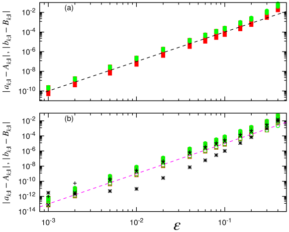
Figure 1: Results for the asynchronous configuration of three coupled Stuart-Landau oscillators, see Eq. (15). Differences between the numerically calculated coupling coefficients and the theoretical values given by Eqs. (22-24) are shown as a function of the coupling strength, for all oscillators. Panel (a) presents this difference for the terms appearing in the 1st order in $\varepsilon$; the black dashed line here corresponds to $\sim\varepsilon^{3}$. Panel (b) presents the terms appearing in the 2nd order in $\varepsilon$; the magenta dashed line here corresponds to $\sim\varepsilon^{4}$. Red squares (green circles) represent cosine (sine) coefficients. Additional black markers in (b) show the differences between the zero-order terms $A_{k;0}$, $k=1,2,3$ and their theoretical values in the second-order approximation.

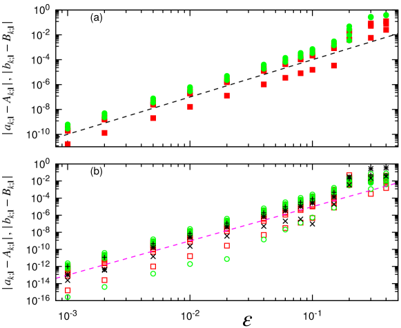
Figure 2: The same as in Fig. 1, but for the synchronous configuration.

We see that for weak coupling the difference is on the level of numerical precision; it becomes of the order of one only for such strong coupling as $\varepsilon=0.4$. Next, we see that the difference for the first-order terms grows proportionally to $\varepsilon^{3}$, in correspondence with our theoretical conclusion that there are no second-order correction to the first-order terms. Thus, numerical results exhibit a good correspondence with the theory.

Figures 3,4 present an overview of all Fourier coefficients for which we do not have theoretical values. Namely, we show here all coefficients except for those entering Eqs. (22-24) and analyzed in Figs. 1,2. The results are in full agreement with the power-series representation of the coupling terms. Indeed, we see four groups of coefficients that scale as $\varepsilon^{3}$, $\varepsilon^{4}$, $\varepsilon^{5}$ and $\varepsilon^{6}$, respectively.

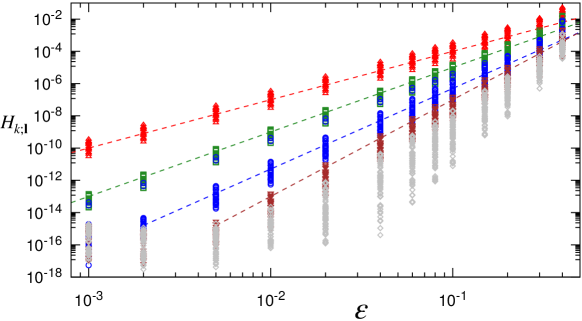
Figure 3: Results for the asynchronous configuration of three coupled Stuart-Landau oscillators, see Eq. (15). Here amplitudes $H_{k;\mathbf{l}}=\sqrt{A_{k;\mathbf{l}}^{2}+B_{k;\mathbf{l}}^{2}}$ of all Fourier coefficients for all three oscillators except for those shown in Fig. 1 are plotted vs. the coupling strength. Red triangles up, green squares, blue circles, and brown triangles down show the coefficients that scale as $\varepsilon^{3}$, $\varepsilon^{4}$, $\varepsilon^{5}$, and $\varepsilon^{6}$, respectively. (The dashed lines, from top to bottom, have slopes 3, 4, 5, and 6 in log-log coordinates.) We did not checked for scaling $\sim\varepsilon^{7}$ and higher, and show all the coupling coefficients that do not fulfill above scaling laws with gray diamonds.

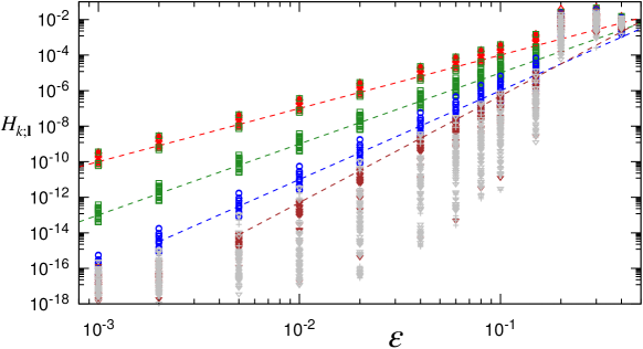
Figure 4: The same as in Fig. 3, but for the synchronous configuration.

Finally, we mention that the overall precision of the numerical procedure can be estimated by computing the rest term $\xi_{k}$ of the Fourier series representation in Eq. (28). The results presented in Fig. 5 show that the rest term grows with the coupling strength as $\varepsilon^{9}$. This is an indication that all the terms of orders from $0$ to $8$ are within the set of chosen Fourier modes.

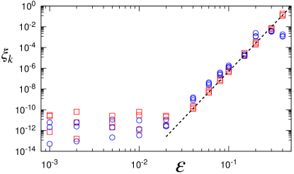
Figure 5: Accuracy of the phase dynamics reconstruction for all oscillators. Red squares and blue circles represent the rest term $\xi_{k}$ of the Fourier representation Eq. (28) for asynchronous and synchronous cases, respectively. The dashed line shows power law $\sim\varepsilon^{9}$.

3.4 A network of van der Pol oscillators

Up to this point, our analysis was restricted to the case of Stuart-Landau oscillators where expressions for phases and their derivatives are known. In this Section we present a purely numerical evaluation of high-order coupling terms for a network of three non-identical van der Pol oscillators:

$$\eqalign{\ddot{x}_{1}&-\mu(1-x_{1}^{2})\dot{x}_{1}+\omega_{1}^{2}x_{1}=\varepsilon x_{2}\\ \ddot{x}_{2}&-\mu(1-x_{2}^{2})\dot{x}_{2}+\omega_{2}^{2}x_{2}=\varepsilon(x_{1}+x_{3})\\ \ddot{x}_{3}&-\mu(1-x_{3}^{2})\dot{x}_{3}+\omega_{3}^{2}x_{3}=\varepsilon x_{2}\\ }$$ (30)

We fixed parameters $\omega_{1}=1$, $\omega_{2}=1.324715957$, $\omega_{3}=\omega_{2}^{2}$ (here $\omega_{2}$ is the spiral mean, the root of cubic equation $\omega_{2}^{3}-\omega_{2}-1=0$). We fixed $\mu=1$ and varied the coupling constant $\varepsilon$ in the range $0.001\leq\varepsilon\leq 0.3$, in this range the dynamics of the network is asynchronous. From a trajectory of the system (30) we obtained time series $\varphi_{1,2,3},\dot{\varphi}_{1,2,3}$ of length $L=10^{6}$ points each. We used this set to estimate the coefficients of the truncated Fourier series in Eq. (28) for $m=4$. Thus, 729 coupling constants $A_{k;\boldsymbol{l}},\;B_{k;\boldsymbol{l}}$ were calculated for each $\varepsilon$. Below we restrict our attention only to the strengths of the coupling and ignore the relative phase, so we look on the properties of 364 coupling constants $H_{k,\boldsymbol{l}}=(A_{k;\boldsymbol{l}}^{2}+B_{k;\boldsymbol{l}}^{2})^{1/2}$. Together with the free term $A_{k;\boldsymbol{0}}$ this constitutes a set of $365$ numerically obtained coefficients for each oscillator and for each coupling constant $\varepsilon$.

For presentation of the results we perform a preliminary sorting. According to the theory, we expect to obtain terms with leading dependencies $\sim\varepsilon^{q}$, with $q=0,1,2,\ldots$. Therefore, for each set of indices $\boldsymbol{l}$ and each oscillator, we tried to approximate the coefficients $H_{k,\boldsymbol{l}}(\varepsilon)$ by the function $\sim\varepsilon^{q}$, and if the fitted value $q$ was close to an integer and the reliability of the fit was high, we attributed the corresponding power to the coupling term. Additionally, for $\varepsilon^{0},\varepsilon,\varepsilon^{2}$ we used the five small values of $\varepsilon=0.001,\;0.002,\;0.005,\;0.01,\;0.02$, while for powers $\varepsilon^{3}$ and $\varepsilon^{4}$ we used larger coupling constants $\varepsilon=0.04,\;0.06,\;0.08,\;0.1,\;0.15$. We did not look for powers $5$ and larger.

Figure 6 illustrates these findings. It is instructive to look which coupling modes appear in each power of $\varepsilon$. For modes up to $\sim\varepsilon^{2}$ we summarize this in Table 1. The modes $A_{k;\boldsymbol{0}}$, describing corrections to the natural frequency are not listed. Notice that in each cell of the table the modes are ordered according to their amplitudes. Below we summarize the properties of the coupling modes of the van der Pol oscillators:

1. Looking at the modes that appear in the first order in $\varepsilon$, we notice that the terms with phase differences and the terms with phase sums have nearly the same amplitude. This means that the coupling terms $\sim\varepsilon$ have nearly the Winfree form: they are products of two functions of the oscillator phase and of the driving oscillator phase, in full agreement with the first-order theory. Recall that it is different for the Stuart-Landau oscillators, where only terms with phase differences appear due to the condition (29).

2. Because the variable $x$ of the van der Pol equation possesses odd harmonics of the phase (and the same is true for the phase response curve), terms with the third harmonics appear already in the 1st order in $\varepsilon$.

3. Inspection of terms $\sim\varepsilon$ in Table 1 reveals some terms that are not expected in the first-order analysis, we show them in italic font. Data in Fig. 6 show that the amplitudes of these terms are extremely small, comparable to the errors in terms reconstruction. We conclude that these terms are probably spurious and just occasionally possess a scaling $\sim\varepsilon$, what is not surprising due to the fact that the total number of terms to be found is large.

4. With the size of the time series explored, we could not reliably detect coupling terms appearing in order $\varepsilon^{5}$. However, as the figures show, the terms $\sim 4$ can be detected with good confidence.

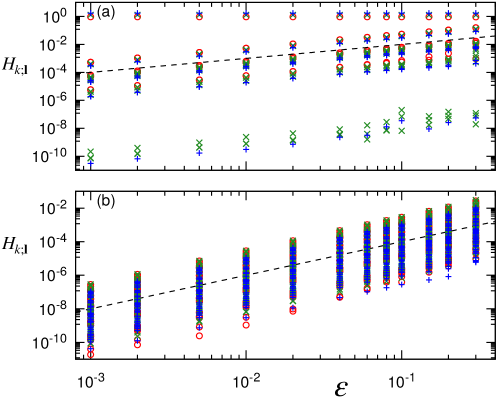
Figure 6: Coupling coefficients $H_{k,\boldsymbol{l}}=(A_{k;\boldsymbol{l}}^{2}+B_{k;\boldsymbol{l}}^{2})^{1/2}$ for all three oscillators are shown by red circles, green crosses, and blue pluses, respectively, vs coupling strength $\varepsilon$. Panel (a) shows powers $0$ and $1$, and panel (b) shows power $2$. Dashed black lines correspond to the scaling $\sim\varepsilon$ and $\sim\varepsilon^{2}$, respectively.

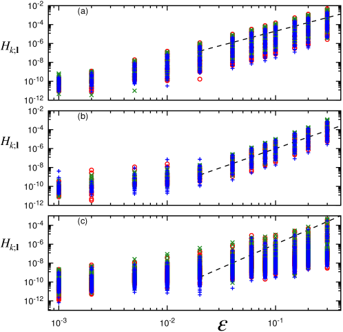
Figure 7: The same as Fig. 6, but for powers $3$ (a) and $4$ (b). Panel (c) presents all other coefficients. Dashed black lines show powers 3,4, and 5, respectively.

Osc	$\varepsilon$	$\varepsilon^{2}$
1	8 Modes: (1,-1,0), (1,1,0), (3,-1,0), (3,1,0), (1,3,0), (1,-3,0), (3,-3,0), (3,3,0)	47 Modes: (2,-2,0), (2,0,0), (0,2,0), (1,-2,1), (1,2,-1), (1,0,-1), (1,0,1), (2,2,0), (1,-2,-1), (1,2,1), (2,-4,0), (1,-4,1), (1,4,-1), (0,4,0), (4,-2,0), (2,4,0), (3,-2,1), (3,2,-1), (3,-2,-1), (3,0,1), (1,4,1), (3,-4,1), (4,2,0), (4,-4,0), (3,0,-1), (1,-4,-1), (3,-4,-1), (4,0,0), (3,2,1), (3,4,-1), (4,4,0), (1,2,-3), (1,0,-3), (1,-2,3), (3,4,1), (1,0,3), (1,2,3), (1,-2,-3), (3,-2,-3), (3,-4,-3), (3,-2,3), (1,1,-4), (3,0,-3), (1,4,3), (3,2,-3), (1,-4,-3), (3,2,3)
2	19 Modes: (0,1,-1), (1,1,0), (0,1,1), (1,-1,0), (3,1,0), (3,-1,0), (0,3,1), (0,1,-3), (0,1,3), (1,3,0), (1,-3,0), (3,-3,0), (0,3,-3), (3,3,0), (0,3,3), (1,2,0), (3,4,0), (2,1,4)	56 Modes: (0,2,0), (2,-2,0), (1,-2,1), (0,2,-2), (2,0,0), (1,0,1), (1,0,-1), (1,-2,-1), (0,0,2), (1,2,-1), (1,2,1), (2,2,0), (4,-2,0), (0,2,2), (4,0,0), (4,2,0), (0,2,-4), (3,0,1), (3,0,-1), (0,0,4), (1,-4,1), (1,-2,3), (3,2,-1), (1,2,-3), (1,4,-1), (1,-2,-3), (1,0,-3), (0,4,-2), (0,2,4), (1,-4,-1), (3,-2,1), (2,4,0), (3,-2,-1), (1,-4,3), (0,4,0), (1,4,1), (1,2,3), (1,0,3), (2,-4,0), (3,4,-1), (4,-4,0), (0,4,2), (3,2,1), (3,-4,1), (3,0,-3), (3,-2,-3), (0,4,-4), (4,4,0), (1,4,-3), (3,-2,3), (3,0,3), (1,-4,-3), (0,4,4), (1,4,3), (3,-4,-3), (3,2,3)
3	9 Modes: (0,1,1), (0,1,-1), (0,3,1), (0,3,-1), (0,1,3), (0,1,-3), (0,3,-3), (0,3,3), (1,-1,1)	50 Modes: (0,2,-2), (0,0,2), (1,0,-1), (1,0,1), (1,-2,-1), (1,-2,1), (0,2,0), (1,2,1), (1,2,-1), (0,2,2), (0,4,-2), (1,-4,-1) , (1,-4,1), (0,4,0), (1,4,1), (1,4,-1), (0,4,2), (3,-2,-1), (3,-4,-1), (1,0,3), (3,-2,1), (3,-4,1), (1,0,-3), (1,-2,-3), (1,-2,3), (0,2,-4), (1,2,3), (1,-4,3), (1,2,-3), (0,2,4) , (3,2,1), (3,2,-1), (3,0,-1), (0,0,4), (3,0,1), (1,4,-3), (1,-4,-3), (1,4,3), (3,-2,-3), (0,4,-4), (3,4,1), (3,-2,3), (0,4,4), (3,4,-1), (3,-4,3), (3,0,3), (3,2,3), (3,2,-3), (3,0,-3), (3,4,3)

Table 1: All modes revealed in orders $\varepsilon$ and $\varepsilon^{2}$ for a network of van der Pol oscillators. Italic font in the second column denotes the modes that shall not appear in the first-order approximation.

4 Conclusion

In this work, we have presented an analytic perturbation approach, allowing the derivation of the equations for the phase dynamics for general networks of Stuart-Landau oscillators. We exemplified this framework with calculations for a particular system of three units. We demonstrated explicitly that already in the second order in coupling strength, there exist coupling terms that are not present in the structural coupling configuration. This result confirms a general statement that phase connectivity generally differs from the structural connectivity of a network. In particular, in higher-order approximation we find triplet coupling terms, which are characteristic for a hypernetwork.

Since analytic derivations of the phase dynamics equations for generic oscillators remain a theoretical challenge, we developed a numerical method to compute the phase dynamics of an oscillatory network and to extract the coupling terms from time series of the obtained phases. These data could be one long trajectory if the dynamics is quasiperiodic, or multiple small pieces (or points) if the dynamics is synchronous. The result of the numerical procedure is a set of Fourier modes of the coupling functions. Analysing these sets for different coupling strengths, we found terms with various power-law dependencies on this strength. We first tested this approach on the coupled Stuart-Landau oscillators, where we demonstrated an excellent agreement with the theory. This numerical approach has also been applied to a network of van der Pol oscillators, coupling functions of which are much more involved.

Appendix A Second-order coupling coefficients in a network of Stuart-Landau oscillators.

Here we present the coefficients for $\dot{\varphi}_{1,2,3}$ in Eqs. (22-24). In Tables 2, 3, 4 we use the notation

$$C_{m,k}=\frac{1+\alpha^{2}}{2}\frac{2c_{m,k}}{4+(\omega_{m}-\omega_{k})^{2}},\qquad D_{m,k}=\frac{1+\alpha^{2}}{2}\frac{(\omega_{m}-\omega_{k})c_{m,k}}{4+(\omega_{m}-\omega_{k})^{2}}\;.$$

$a^{(2)}_{1;0}$	$c_{2,1}\Big{(}C_{1,2}\sin(\beta_{1,2}+\beta_{2,1})-D_{1,2}\cos(\beta_{1,2}+\beta_{2,1})-D_{2,1}\Big{)}$
$a^{(2)}_{1;-2,2,0}$	$c_{2,1}\Big{(}C_{1,2}\sin(\beta_{2,1}-\beta_{1,2})+D_{1,2}\cos(\beta_{2,1}-\beta_{1,2})$
	$-C_{2,1}\sin 2\beta_{2,1}+D_{2,1}\cos 2\beta_{2,1}\Big{)}$
$b^{(2)}_{1;-2,2,0}$	$c_{2,1}\Big{(}C_{1,2}\cos(\beta_{2,1}-\beta_{1,2})-D_{1,2}\sin(\beta_{2,1}-\beta_{1,2})$
	$-C_{2,1}\cos 2\beta_{2,1}-D_{2,1}\sin 2\beta_{2,1}\Big{)}$
$a^{(2)}_{1;-1,2,-1}$	$c_{2,1}\Big{(}C_{3,2}\sin(\beta_{2,1}-\beta_{3,2})+D_{3,2}\cos(\beta_{2,1}-\beta_{3,2})\Big{)}$
$b^{(2)}_{1;-1,2,-1}$	$c_{2,1}\Big{(}C_{3,2}\cos(\beta_{2,1}-\beta_{3,2})-D_{3,2}\sin(\beta_{2,1}-\beta_{3,2})\Big{)}$
$a^{(2)}_{1;-1,0,1}$	$c_{2,1}\Big{(}-D_{3,2}\cos(\beta_{2,1}+\beta_{3,2})+C_{3,2}\sin(\beta_{2,1}+\beta_{3,2})\Big{)}$
$b^{(2)}_{1;-1,0,1}$	$c_{2,1}\Big{(}D_{3,2}\sin(\beta_{2,1}+\beta_{3,2})+C_{3,2}\cos(\beta_{2,1}+\beta_{3,2})\Big{)}$

Table 2: Coupling coefficients of the first Stuart-Landau oscillator.

$a^{(2)}_{2;0}$	$\Big{(}C_{2,1}c_{1,2}\sin(\beta_{2,1}+\beta_{1,2})-D_{2,1}c_{1,2}\cos(\beta_{2,1}+\beta_{1,2})-D_{1,2}c_{1,2}$
	$+C_{2,3}c_{3,2}\sin(\beta_{3,2}+\beta_{2,3})-D_{3,2}c_{3,2}-D_{2,3}c_{3,2}\cos(\beta_{3,2}+\beta_{2,3})\Big{)}$
$a^{(2)}_{2;2,-2,0}$	$\Big{(}C_{2,1}c_{1,2}\sin(\beta_{1,2}-\beta_{2,1})+D_{2,1}c_{1,2}\cos(\beta_{1,2}-\beta_{2,1})$
	$-C_{1,2}c_{1,2}\sin 2\beta_{1,2}+D_{1,2}c_{1,2}\cos 2\beta_{1,2}\Big{)}$
$b^{(2)}_{2;2,-2,0}$	$\Big{(}C_{2,1}c_{1,2}\cos(\beta_{1,2}-\beta_{2,1})-D_{2,1}c_{1,2}\sin(\beta_{1,2}-\beta_{2,1})$
	$-C_{1,2}c_{1,2}\cos 2\beta_{1,2}-D_{1,2}c_{1,2}\sin 2\beta_{1,2}\Big{)}$
$a^{(2)}_{2;0,-2,2}$	$\Big{(}C_{2,3}c_{3,2}\sin(\beta_{3,2}-\beta_{2,3})+D_{2,3}c_{3,2}\cos(\beta_{3,2}-\beta_{2,3})$
	$-C_{3,2}c_{3,2}\sin 2\beta_{3,2}+D_{3,2}c_{3,2}\cos 2\beta_{3,2}\Big{)}$
$b^{(2)}_{2;0,-2,2}$	$\Big{(}C_{2,3}c_{3,2}\cos(\beta_{3,2}-\beta_{2,3})-D_{2,3}c_{3,2}\sin(\beta_{3,2}-\beta_{2,3})$
	$-C_{3,2}c_{3,2}\cos 2\beta_{3,2}-D_{3,2}c_{3,2}\sin 2\beta_{3,2}\Big{)}$
$a^{(2)}_{2;-1,2,-1}$	$\Big{(}D_{3,2}c_{1,2}\cos(\beta_{1,2}+\beta_{3,2})-C_{3,2}c_{1,2}\sin(\beta_{1,2}+\beta_{3,2})$
	$-C_{1,2}c_{3,2}\sin(\beta_{3,2}+\beta_{1,2})+D_{1,2}c_{3,2}\cos(\beta_{3,2}+\beta_{1,2})\Big{)}$
$b^{(2)}_{2;-1,2,-1}$	$\Big{(}D_{3,2}c_{1,2}\sin(\beta_{1,2}+\beta_{3,2})+C_{3,2}c_{1,2}\cos(\beta_{1,2}+\beta_{3,2})$
	$+C_{1,2}c_{3,2}\cos(\beta_{3,2}+\beta_{1,2})+D_{1,2}c_{3,2}\sin(\beta_{3,2}+\beta_{1,2})\Big{)}$
$a^{(2)}_{2;1,0,-1}$	$\Big{(}-D_{3,2}c_{1,2}\cos(\beta_{1,2}-\beta_{3,2})-C_{3,2}c_{1,2}\sin(\beta_{1,2}-\beta_{3,2})$
	$-C_{1,2}c_{3,2}\sin(\beta_{3,2}-\beta_{1,2})-D_{1,2}c_{3,2}\cos(\beta_{3,2}-\beta_{1,2})\Big{)}$
$b^{(2)}_{2;1,0,-1}$	$\Big{(}D_{3,2}c_{1,2}\sin(\beta_{1,2}-\beta_{3,2})-C_{3,2}c_{1,2}\cos(\beta_{1,2}-\beta_{3,2})$
	$+C_{1,2}c_{3,2}\cos(\beta_{3,2}-\beta_{1,2})-D_{1,2}c_{3,2}\sin(\beta_{3,2}-\beta_{1,2})\Big{)}$

Table 3: Coupling coefficients of the second Stuart-Landau oscillator.

$a^{(2)}_{3;0}$	$c_{2,3}\Big{(}C_{3,2}\sin(\beta_{3,2}+\beta_{2,3})-D_{3,2}\cos(\beta_{3,2}+\beta_{2,3})-D_{2,3}\Big{)}$
$a^{(2)}_{3;0,2,-2}$	$c_{2,3}\Big{(}C_{3,2}\sin(\beta_{2,3}-\beta_{3,2})+D_{3,2}\cos(\beta_{2,3}-\beta_{3,2})$
	$-C_{2,3}\sin 2\beta_{2,3}+D_{2,3}\cos 2\beta_{2,3}\Big{)}$
$b^{(2)}_{3;0,2,-2}$	$c_{2,3}\Big{(}C_{3,2}\cos(\beta_{2,3}-\beta_{3,2})-D_{3,2}\sin(\beta_{2,3}-\beta_{3,2})$
	$-C_{2,3}\cos 2\beta_{2,3}-D_{2,3}\sin 2\beta_{2,3}\Big{)}$
$a^{(2)}_{3;-1,2,-1}$	$c_{2,3}\Big{(}C_{1,2}\sin(\beta_{2,3}-\beta_{1,2})+D_{1,2}\cos(\beta_{2,3}-\beta_{1,2})\Big{)}$
$b^{(2)}_{3;-1,2,-1}$	$c_{2,3}\Big{(}C_{1,2}\cos(\beta_{2,3}-\beta_{1,2})-D_{1,2}\sin(\beta_{2,3}-\beta_{1,2})\Big{)}$
$a^{(2)}_{3;1,0,-1}$	$c_{2,3}\Big{(}-D_{1,2}\cos(\beta_{2,3}+\beta_{1,2})+C_{1,2}\sin(\beta_{2,3}+\beta_{1,2})\Big{)}$
$b^{(2)}_{3;1,0,-1}$	$c_{2,3}\Big{(}D_{1,2}\sin(\beta_{2,3}+\beta_{1,2})+C_{1,2}\cos(\beta_{2,3}+\beta_{1,2})\Big{)}$

Table 4: Coupling coefficients of the third Stuart-Landau oscillator.

Appendix B Terms in the higher orders for coupled Stuart-Landau oscillators

In Table 5 we present coupling modes appearing in higher orders in $\varepsilon$. Namely, we just give the vectors $\boldsymbol{l}$ of these modes. Up to order $4$ we checked all of them both analytically and numerically; for order $5$ we present only numerical results.

	1 and 3	2 and 4	3	4	5
1	(-1,1,0)	(0,0,0)	(-3,3,0), (0,-1,1)	(-4,4,0), (0,-2,2)	(0,3,-3), (5,-5,0)
		(-2,2,0)	(-1,3,-2), (-2,3,-1)	(-2,0,2), (2,-4,2)	(2,-5,3), (3,-5,2)
		(-1,0,1)	(-1,-1,2), (-2,1,1)	(-1,-2,3), (3,-2,-1)	(3,-1,-2), (2,1,-3)
		(1,-2,1)		(-1,4,-3), (-3,4,-1)	(4,-5,1), (1,-5,4)
					(4,-3,-1), (1,3,-4)
2	(1,-1,0)	(0,0,0)	(-3,3,0), (0,3,-3)	(-4,4,0), (0,4,-4)	(5,-5,0), (0,5,-5)
	(0,-1,1)	(2,-2,0)	(-1,3,-2), (-2,3,-1)	(-2,0,2), (2,-4,2)	(3,-1,-2), (1,2,-3)
		(0,-2,2)	(-1,-1,2), (-2,1,1)	(-1,-2,3), (3,-2,-1)	(1,3,-4), (4,-3,-1)
		(-1,0,1)		(-1,4,-3), (-3,4,-1)	(4,-5,1), (1,-5,4)
		(1,-2,1)		(2,-5,3), (3,-5,2)	(3,-5,2), (2,-5,3)
3	(0,1,-1)	(0,0,0)	(0,3,-3), (1,-1,0)	(0,4,-4), (2,-2,0)	(3,-3,0), (0,5,-5)
		(0,2,-2)	(-1,3,-2), (-2,3,-1)	(2,0,-2), (2,-4,2)	(3,-5,2), (2,-5,3)
		(1,0,-1)	(-1,-1,2), (-2,1,1)	(-1,-2,3), (3,-2,-1)	(3,-1,-2), (2,1,-3)
		(1,-2,1)		(-1,4,-3), (-3,4,-1)	(1,-5,4), (4,-5,1)
					(1,3,-4), (4,-3,-1)

Table 5: Coupling terms that appear in different orders (see columns) and for all three oscillators (see rows).

Appendix C Numerical reconstruction of coupling for Stuart-Landau oscillators: approach (ii)

Here we present the result of the numerical procedure using the approach (ii), i.e. here we do not exclude zero modes that do not fulfill the condition (29). Comparison of this case with the results for the approach (i), presented in the main text, is important for the analysis of networks of van der Pol or other oscillators, for which no modes can be excluded a priori. Figures 8-12 shall be compared to Figs. 1-5, respectively. The comparison shows that the results are consistent. As expected, the approach (i) provides a higher accuracy since fewer unknowns shall be found. However, even with the second approach, we managed to reliably reveal scaling of the mode coefficients up to the order $\sim\varepsilon^{5}$.

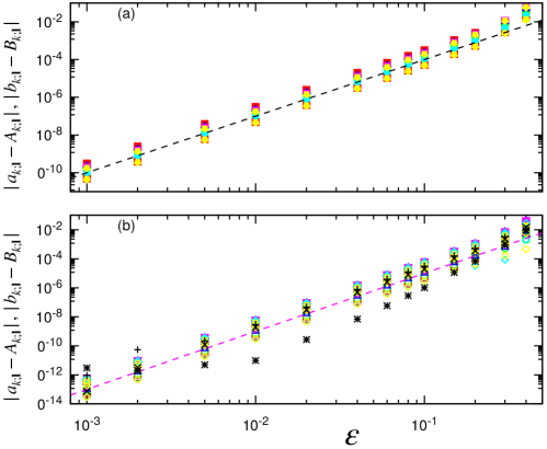
Figure 8: Results for the asynchronous configuration (case I) of three coupled Stuart-Landau oscillators, see Eq.(15). Differences between the numerically calculated coupling coefficients and the theoretical values given by Eqs.(22-24) are shown as a function of the coupling strength, for all oscillators. Panel (a) presents this difference for the terms appearing in the 1st order in $\varepsilon$; the black dashed line here corresponds to $\sim\varepsilon^{3}$. Panel (b) presents the terms appearing in the 2nd order in $\varepsilon$; the magenta dashed line here corresponds to $\sim\varepsilon^{4}$. Red squares (green circles) represent cosine (sine) coefficients. Additional black markers in (b) show the differences between the zero-order terms $A_{k;0}$, $k=1,2,3$ and their theoretical values in the second-order approximation.

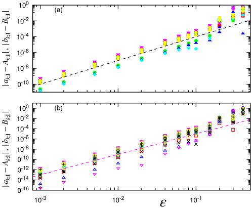
Figure 9: The same as in Fig. 8, but for the synchronous configuration.

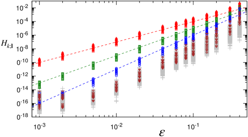
Figure 10: Results for the asynchronous configuration (case I) of three coupled Stuart-Landau oscillators, see Eq. (15). Here all Fourier coefficients for all three oscillators except for those shown in Fig. 8 are plotted vs. the coupling strength. Red triangles up, green squares, blue circles, and brown triangles down show the coefficients that scale as $\varepsilon^{3}$, $\varepsilon^{4}$, and $\varepsilon^{5}$, respectively. (The dashed lines, from top to bottom, have slopes 3, 4, and 5, in log-log coordinates.) We did not checked for scaling $\sim\varepsilon^{6}$ and higher, and show all the coupling coefficients that do not fulfill above scaling laws with gray pluses.

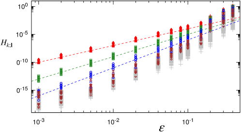
Figure 11: The same as in Fig. 10, but for the synchronous configuration.

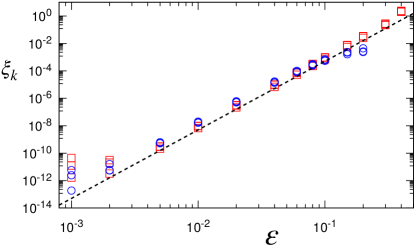
Figure 12: Accuracy of the phase dynamics reconstruction. Red squares and blue circles illustrate asynchronous and synchronous cases, respectively. The dashed line shows power law $\sim\varepsilon^{5}$.

References

- [1] Micha Nixon, Eitan Ronen, Asher A. Friesem, and Nir Davidson. Observing geometric frustration with thousands of coupled lasers. Phys. Rev. Lett., 110:184102, 2013.
- [2] M. H. Matheny, M. Grau, L. G. Villanueva, R. B. Karabalin, M. C. Cross, and M. L. Roukes. Phase synchronization of two anharmonic nanomechanical oscillators. Phys. Rev. Lett., 112:014101, 2014.
- [3] Balth. van der Pol and J. van der Mark. The heartbeat considered as a relaxation oscillation, and an electrical model of the heart. The London, Edinburgh, and Dublin Philosophical Magazine and Journal of Science, 6(38):763–775, 1928.
- [4] I Ashraf, R Godoy-Diana, J Halloy, B Collignon, and B Thiria. Synchronization and collective swimming patterns in fish (hemigrammus bleheri). Journal of the Royal Society Interface, 13(123):20160734, 2016.
- [5] Steven H Strogatz, Daniel M Abrams, Allan McRobie, Bruno Eckhardt, and Edward Ott. Theoretical mechanics: Crowd synchrony on the Millennium Bridge. Nature, 438(7064):43–44, 2005.
- [6] Florian Dörfler and Francesco Bullo. Synchronization in complex networks of phase oscillators: A survey. Automatica, 50(6):1539–1564, 2014.
- [7] J. García-Ojalvo, J. Casademont, and M. C. Torrent. Coherence and synchronization in diode-laser arrays with delayed global coupling. Int. J. of Bifurcation and Chaos, 9(11):2225–2229, 1999.
- [8] M. H. Matheny, J. Emenheiser, W. Fon, A. Chapman, A. Salova, M. Rohden, J. Li, M. Hudoba de Badyn, M. P’osfai, L. Duenas-Osorio, M. Mesbahi, J. P. Crutchfield, M. C. Cross, R. M. D’Souza, and M. L. Roukes. Exotic states in a simple network of nanoelectromechanical oscillators. Science, 363:eaav7932, 2019.
- [9] A. B. Cawthorne, P. Barbara, S. V. Shitov, C. J. Lobb, K. Wiesenfeld, and A. Zangwill. Synchronized oscillations in Josephson junction arrays: The role of distributed coupling. Phys. Rev. B, 60:7575–7578, 1999.
- [10] V. Tiberkevich, A. Slavin, E. Bankowski, and G. Gerhart. Phase-locking and frustration in an array of nonlinear spin-torque nano-oscillators. Appl. Phys. Lett., 95:262505, 2009.
- [11] A. E. Motter, S. A. Myers, M. Anghel, and T. Nishikawa. Spontaneous synchrony in power-grid networks. Nat. Phys., 9:191, 2013.
- [12] Peter Uhlhaas, Gordon Pipa, Bruss Lima, Lucia Melloni, Sergio Neuenschwander, Danko Nikolić, and Wolf Singer. Neural synchrony in cortical networks: history, concept and current status. Frontiers in Integrative Neuroscience, 3:17, 2009.
- [13] L. Glass. Synchronization and rhythmic processes in physiology. Nature, 410:277–284, 2001.
- [14] A. Prindle, P. Samayoa, I. Razinkov, T. Danino, L. S. Tsimring, and J. Hasty. A sensing array of radically coupled genetic “biopixels”. Nature, 481(7379):39–44, 2012.
- [15] Yoshiki Kuramoto. Chemical oscillations, turbulence and waves. Springer, Berlin, 1984.
- [16] Arkady Pikovsky, Jurgen Kurths, Michael Rosenblum, and Jürgen Kurths. Synchronization: a universal concept in nonlinear sciences. Cambridge University Press, 2001.
- [17] Hiroya Nakao. Phase reduction approach to synchronisation of nonlinear oscillators. Contemporary Physics, 57(2):188–214, 2016.
- [18] Bastian Pietras and Andreas Daffertshofer. Network dynamics of coupled oscillators and phase reduction techniques. Physics Reports, 2019.
- [19] Y. Kuramoto. Self-entrainment of a population of coupled nonlinear oscillators. In H. Araki, editor, International Symposium on Mathematical Problems in Theoretical Physics, page 420, New York, 1975. Springer Lecture Notes Phys., v. 39.
- [20] J. A. Acebrón, L. L. Bonilla, C. J. Pérez Vicente, F. Ritort, and R. Spigler. The Kuramoto model: A simple paradigm for synchronization phenomena. Rev. Mod. Phys., 77(1):137–175, 2005.
- [21] Iván León and Diego Pazó. Phase reduction beyond the first order: The case of the mean-field complex Ginzburg-Landau equation. Physical Review E, 100(1):012211, 2019.
- [22] Dan Wilson and Jeff Moehlis. Isostable reduction of periodic orbits. Physical Review E, 94(5):052213, 2016.
- [23] Hiroaki Daido. Order function and macroscopic mutual entrainment in uniformly coupled limit-cycle oscillators. Progress of Theoretical Physics, 88(6):1213–1218, 1992.
- [24] Michael Rosenblum and Arkady Pikovsky. Self-organized quasiperiodicity in oscillator ensembles with global nonlinear coupling. Physical Review Letters, 98(6):064101, 2007.
- [25] Wataru Kurebayashi, Sho Shirasaka, and Hiroya Nakao. Phase reduction method for strongly perturbed limit cycle oscillators. Physical Review Letters, 111(21), November 2013.
- [26] Kestutis Pyragas and Viktor Novičenko. Phase reduction of a limit cycle oscillator perturbed by a strong amplitude-modulated high-frequency force. Physical Review E, 92(1), July 2015.
- [27] Erik Gengel and Arkady Pikovsky. Phase demodulation with iterative Hilbert transform embeddings. Signal Processing, 165:115–127, 2019.
- [28] Rok Cestnik and Michael Rosenblum. Inferring the phase response curve from observation of a continuously perturbed oscillator. Scientific reports, 8(1):1–10, 2018.
- [29] Björn Kralemann, Laura Cimponeriu, Michael Rosenblum, Arkady Pikovsky, and Ralf Mrowka. Phase dynamics of coupled oscillators reconstructed from data. Physical Review E, 77(6), June 2008.
- [30] B. Bezruchko, V. Ponomarenko, M. G. Rosenblum, and A. S. Pikovsky. Characterizing direction of coupling from experimental observations. CHAOS, 13(1):179–184, 2003.
- [31] I. T. Tokuda, S. Jain, I. Z. Kiss, and J. L. Hudson. Inferring phase equations from multivariate time series. Phys. Rev. Lett., 99:064101, 2007.
- [32] K. A. Blaha, A. Pikovsky, M. Rosenblum, M. T. Clark, C. G. Rusin, and J. L. Hudson. Reconstruction of two-dimensional phase dynamics from experiments on coupled oscillators. Phys. Rev. E, 84:046201, 2011.
- [33] B. Kralemann, M. Frühwirth, A. Pikovsky, M. Rosenblum, T. Kenner, J. Schaefer, and M. Moser. In vivo cardiac phase response curve elucidates human respiratory heart rate variability. Nature Communications, 4:2418, 2013.
- [34] M. Rosenblum, M. Frühwirth, M. Moser, and A. Pikovsky. Dynamical disentanglement in an analysis of oscillatory systems: an application to respiratory sinus arrhythmia. Philosophical Transactions of the Royal Society A: Mathematical, Physical and Engineering Sciences, 377(2160):20190045, 2019.
- [35] Valentina Ticcinelli, Tomislav Stankovski, Dmytro Iatsenko, Alan Bernjak, Adam E Bradbury, Andrew R Gallagher, Peter Clarkson, Peter VE McClintock, and Aneta Stefanovska. Coherence and coupling functions reveal microvascular impairment in treated hypertension. Frontiers in physiology, 8:749, 2017.
- [36] Çağdaş Topçu, Matthias Frühwirth, Maximilian Moser, Michael Rosenblum, and Arkady Pikovsky. Disentangling respiratory sinus arrhythmia in heart rate variability records. Physiological measurement, 39(5):054002, 2018.
- [37] Tomislav Stankovski, Tiago Pereira, Peter VE McClintock, and Aneta Stefanovska. Coupling functions: universal insights into dynamical interaction mechanisms. Reviews of Modern Physics, 89(4):045001, 2017.
- [38] Tomislav Stankovski, Spase Petkoski, Johan Raeder, Andrew F Smith, Peter VE McClintock, and Aneta Stefanovska. Alterations in the coupling functions between cortical and cardio-respiratory oscillations due to anaesthesia with propofol and sevoflurane. Philosophical Transactions of the Royal Society A: Mathematical, Physical and Engineering Sciences, 374(2067):20150186, 2016.
- [39] Björn Kralemann, Arkady Pikovsky, and Michael Rosenblum. Reconstructing phase dynamics of oscillator networks. Chaos: An Interdisciplinary Journal of Nonlinear Science, 21(2):025104, 2011.
- [40] Björn Kralemann, Arkady Pikovsky, and Michael Rosenblum. Reconstructing effective phase connectivity of oscillator networks from observations. New Journal of Physics, 16(8):085013, August 2014.
- [41] M. Komarov and A. Pikovsky. Finite-size-induced transitions to synchrony in oscillator ensembles with nonlinear global coupling. Phys. Rev. E, 92:020901, 2015.
- [42] C. C. Gong and A. Pikovsky. Low-dimensional dynamics for higher-order harmonic, globally coupled phase-oscillator ensembles. Phys. Rev. E, 100:062210, 2019.
- [43] Michael Rosenblum and Arkady Pikovsky. Numerical phase reduction beyond the first order approximation. Chaos: An Interdisciplinary Journal of Nonlinear Science, 29(1):011105, 2019.
- [44] William H Press, Saul A Teukolsky, William T Vetterling, and Brian P Flannery. Numerical recipes: The art of scientific computing (3rd edition). Cambridge university press, 2007.
- [45] Z. Levnajić and A. Pikovsky. Network reconstruction from random phase resetting. Phys. Rev. Lett., 107(3):034101, 2011.
- [46] A. Pikovsky. Reconstruction of a random phase dynamics network from observations. Physics Letters A, 382(4):147 – 152, 2018.
- [47] Björn Kralemann, Arkady Pikovsky, and Michael Rosenblum. Detecting triplet locking by triplet synchronization indices. Physical Review E, 87(5), May 2013.
- [48] Hannes Osterhage, Florian Mormann, Tobias Wagner, and Klaus Lehnertz. Measuring the directionality of coupling: phase versus state space dynamics and application to EEG time series. International journal of neural systems, 17(03):139–148, 2007.
- [49] Thorsten Rings and Klaus Lehnertz. Distinguishing between direct and indirect directional couplings in large oscillator networks: Partial or non-partial phase analyses? Chaos: An Interdisciplinary Journal of Nonlinear Science, 26(9):093106, September 2016.