Convergence of the Kiefer-Wolfowitz algorithm in the presence of discontinuities

Abstract

In this paper we estimate the expected error of a stochastic approximation algorithm where the maximum of a function is found using finite differences of a stochastic representation of that function. An error estimate of the order $n^{-1/5}$ for the $n$th iteration is achieved using suitable parameters. The novelty with respect to previous studies is that we allow the stochastic representation to be discontinuous and to consist of possibly dependent random variables (satisfying a mixing condition).

1 Introduction

We are interested in maximizing a function $U:\mathbb{R}^{d}\to\mathbb{R}$ which is unknown. However, we can observe a sequence $J(\theta,X_{n})$, $n\geq 1$ where $J:\mathbb{R}^{d}\times\mathbb{R}^{m}\to\mathbb{R}$ is measurable,

$$\mathbb{E}[J(\theta,X_{1})]=U(\theta),\ \theta\in\mathbb{R}^{d},$$ (1)

and $X_{n}$, $n\geq 1$ is an $\mathbb{R}^{m}$-valued stationary process in the strong sense. The stochastic representations $J(\theta,X_{n})$ are often interpreted as noisy measurements of $U(\theta)$. In this paper we focus on applications to mathematical finance, described in Section 6 below, where $J(\theta,X_{t})$ are functionals of observed economic variables $X_{t}$ and $\theta$ determines an investor’s portfolio strategy. In that context, stochasticity does not come from measurement errors but it is an intrinsic property of the system. Maximizing $U$ serves to find the best investment policy in an online, adaptive manner.

We study a recursive algorithm employing finite differences, as proposed by Kiefer and Wolfowitz in [14]. This is a variant of the Robbins-Monro stochastic gradient method [19] where, instead of the objective function itself, its gradient is assumed to admit a stochastic representation.

The novelty in our work is that we do not assume differentiability, not even continuity of $\theta\to J(\theta,\cdot)$ and the sequence $X_{n}$ may well be dependent as long as it satisfies a mixing condition. The only result in such a setting that we are aware of is in [16], however, they only study almost sure convergence, without a convergence rate. Our purpose is not to find the weakest possible hypotheses but to arouse keen interest in the given problem that can lead to further, more general results. Our work is also a continuation of [7, 4], where discontinuous stochastic gradient procedures were treated.

The main theorems are stated in Section 2 and proved in Section 3. Section 4 recalls earlier results that we are relying on. A numerical example is provided in Section 5. We explain the significance of our results for algorithmic trading in Section 6.

2 Setup and results

For real-valued quantities $X,Y$ the notation $O(X)=Y$ means that there is a constant $C>0$ such that $|X|\leq CY$. We will always work on a fixed probability space $(\Omega,\mathcal{F},P)$ equipped with a filtration $\mathcal{F}_{n}$, $n\in\mathbb{N}$ such that $\mathcal{F}_{0}=\{\emptyset,\Omega\}$. A decreasing sequence of sigma-algebras $\mathcal{F}^{+}_{n}$, $n\in\mathbb{N}$ is also given, such that, for each $n\in\mathbb{N}$, $\mathcal{F}_{n}$ and $\mathcal{F}_{n}^{+}$ are independent and $X_{n}$ is adapted to $\mathcal{F}_{n}$. The notation $\mathbb{E}[X]$ refers to the expectation of a real-valued random variable $X$, while $\mathbb{E}_{k}[X]$ is a shorthand notation for $\mathbb{E}[X|\mathcal{F}_{k}]$, $k\in\mathbb{N}$. $P_{k}(A)$ refers to the conditional probability $P(A|\mathcal{F}_{k})$. We denote by $\mathbb{1}_{A}$ the indicator of a set $A$. The notation $\omega$ refers to a generic element of $\Omega$. For $r\geq 1$, we refer to the set of random variables with finite $r$th moments as $L^{r}$. $|\cdot|$ denotes the Euclidean norm in $\mathbb{R}^{k}$ where $k$ may vary according to the context.

For $i=1,\ldots,d$, let $\mathbf{e}_{i}\in\mathbb{R}^{d}$ denote the vector whose $i$th coordinate is $1$ and the other coordinates are $0$. For two vectors $v,w\in\mathbb{R}^{m}$ the relation $v\leq w$ expresses that $v^{i}\leq w^{i}$ for all the components $i=1,\ldots,m$. Let $B_{r}:=\{\theta\in\mathbb{R}^{d}:\,|\theta|\leq r\}$ denote the ball of radius $r$, for $r\geq 0$.

Let the function $U:\mathbb{R}^{d}\to\mathbb{R}$ have a unique maximum at the point $\theta^{*}\in\mathbb{R}^{d}$. Consider the following recursive stochastic approximation scheme for finding $\theta^{*}$:

$$\theta_{k+1}=\theta_{k}+\lambda_{k}H(\theta_{k},X_{k+1},c_{k})\text{, for }k\in\mathbb{N},$$ (2)

starting from some initial (deterministic) guess $\theta_{0}\in\mathbb{R}^{d}$, where $H$ is an estimator of the gradient of $J$, defined as

$$H(\theta,x,c)=\sum_{i=1}^{d}\frac{J(\theta+c\mathbf{e}_{i},x)-J(\theta-c\mathbf{e}_{i},x)}{2c}\mathbf{e}_{i},$$

for all $\theta\in\mathbb{R}^{d}$, $x\in\mathbb{R}^{m}$ and $c>0$.

The sequences $(\lambda_{k})_{k\in\mathbb{N}}$ and $(c_{k})_{k\in\mathbb{N}}$ appearing in (2) will consist of positive real numbers, which are to be specified later. We will distinguish the cases where $\lambda_{k}$, $c_{k}$ tend to zero and where they are kept constant, the former being called decreasing gain approximation and the latter fixed gain approximation.

Remark 2.1.

Our results below could easily be formulated in a more general setting where $J(\theta_{k}+c_{k}\mathbf{e}_{i},X_{k+1}(i))$ and $J(\theta_{k}-c_{k}\mathbf{e}_{i},X_{k+1}^{\prime}(i))$, $i=1,\ldots,d$ are considered with distinct $X_{k+1}(i)$ and $X_{k+1}^{\prime}(i)$. In the applications that motivate us this is not the case hence, for reasons of simplicity, we stay in the present setting.

Assumption 1.

$U$ is continuously differentiable with unique maximum $\theta^{*}\in\mathbb{R}^{d}$. Denote $G(\theta)=\nabla U(\theta)$. The function $G$ is assumed Lipschitz-continuous with Lipschitz-constant $L_{G}$.

We assume in the sequel that the function $J$ in (1) has a specific form. Note that though $J$ is not continuous, $U$ can nonetheless be continuously differentiable, by the smoothing effect of randomness.

Assumption 2.

Let the function $J$ be of the following specific form:

$$J(\theta,x)=l_{0}(\theta)\mathbb{1}_{A_{0}(x)}+{}\sum_{i=1}^{m_{s}}\mathbb{1}_{A_{i}(x)}l_{i}(\theta,x),{}$$

where $l_{i}:\mathbb{R}^{d}\times\mathbb{R}^{m}\to\mathbb{R}^{d}$ are Lipschitz-continuous (in both variables) for $i=1,\ldots,m_{s}$ and, for some $m_{p},m_{p}^{\prime}\in\mathbb{N}$,

$$A_{i}(x):=\left(\cap_{j=1}^{m_{p}}\{\theta:x\leq g_{i}^{j}(\theta)\}\right)\bigcap\left(\cap_{j=1}^{m_{p}^{\prime}}\{\theta:x>h_{i}^{j}(\theta)\}\right),\ i=1,\ldots,m_{s}$$

with Lipschitz-continuous functions $g^{j}_{i},h_{i}^{j}:\mathbb{R}^{d}\to\mathbb{R}^{m}$. Furthermore, $A_{0}(x):=\mathbb{R}^{d}\setminus\cup_{i=1}^{m_{s}}A_{i}(x)$ and

$$\cup_{x\in\mathbb{R}^{m}}\cup_{i=1}^{m_{s}}A_{i}(x)\subset B_{D}$$

for some $D>0$. The function $l_{0}$ is twice continuously differentiable and there are constants $L_{1}^{\prime\prime},L_{2}^{\prime\prime}$ such that

$$L_{1}^{\prime\prime}I\leq\nabla\nabla l_{0}\leq L_{2}^{\prime\prime}I$$

where $I$ is the $d\times d$ identity matrix.

Remark 2.2.

Assumption 2 implies that $\nabla l_{0}$ grows linearly, hence $l_{0}$ itself is locally Lipschitz with linearly growing Lipschitz-coefficient, that is,

$$|l_{0}(\theta_{1})-l_{0}(\theta_{2})|\leq L_{0}(1+|\theta_{1}|+|\theta_{2}|)|\theta_{1}-\theta_{2}|,$$

with some $L_{0}>0$, for all $\theta_{1},\theta_{2}\in\mathbb{R}^{d}$.

In plain English, we consider $J$ which is smooth on a finite number of bounded domains (the interior of the constraint sets $A_{i}(x)$, $i=1,\ldots,m_{s}$) but may have discontinuities at the boundaries. Furthermore, $J$ (and hence also $U$) is required to be quadratic “near infinity” (on $A_{0}(x)$).

We briefly explain why such a hypothesis is not restrictive for real-life applications. Normally, there is a compact set $Q$ (e.g. a cube or a ball) such that only parameters from $Q$ are relevant, i.e. $U$ is defined only on $Q$. Assume it has some stochastic representation

$$U(\theta)=\mathbb{E}[J(\theta,X_{0})],\ \theta\in Q$$ (3)

and a unique maximum $\theta^{*}\in Q$. Assume that $Q\subset B_{D}$ for some $D$. Extend $U$ outside $B_{D}$ as $U(\theta)=-A|\theta|^{2}+B$ for suitable $A,B$. Extend $U$ and $J$ to $B_{D}\setminus Q$ as well in such a way that $U$ is continuously differentiable, $U(\theta)<U(\theta^{*})$ for all $\theta\neq\theta^{*}$ (see Section 4 of [5] for a rigorous construction of this kind). Set $J:=U$ outside $Q$. Then our maximization procedure can be applied to this setting for finding $\theta^{*}$.

Defining $U=l_{0}$ (essentially) quadratic outside a compact set is one way of solving the problem that such procedures often leave their effective domain $Q$. Other solutions are resetting, see e.g. [9]; or an analysis of the probability of divergence, see e.g. [2].

The next assumption postulates that the process $X$ should be bounded and the conditional laws of $X_{k+1}$ should be absolutely continuous with a bounded density.

Assumption 3.

For each $k\in\mathbb{N}$,

$$P_{k}(X_{k+1}\in A)(\omega)=\int_{A}p_{k}(u,\omega)\,du,P\mbox{-a.s.,}A\in\mathcal{B}(\mathbb{R}^{d}),$$

for some measurable $p_{k}:\mathbb{R}^{d}\times\Omega\to\mathbb{R}_{+}$ and there is a fixed constant $F$ such that $p_{k}(u,\omega)\leq F$ holds for all $k$, $\omega$, $u$. The random variable $X_{0}$ satisfies $|X_{0}|\leq K_{0}$ for some constant $K_{0}$.

Note that, by strong stationarity, the process $X_{k}$ is uniformly bounded under Assumption 3.

We will assume a certain mixing property about the process $X_{n}$ which we recall now. A family of $\mathbb{R}^{d}$-valued random variables $Z_{i}$, $i\in\mathcal{I}$ is called $L^{r}$-bounded for some $r\geq 1$ if $\sup_{i\in\mathcal{I}}\mathbb{E}|Z_{i}|^{r}<\infty$, here $\mathcal{I}$ may be an arbitrary index set.

For a random field $Y_{n}(\theta)$, $n\in\mathbb{N}$, $\theta\in\mathbb{R}^{d}$ bounded in $L^{r}$ for some $r\geq 1$, we define, for all $n\in\mathbb{N}$,

$$M_{r}^{n}(Y)=\operatorname*{ess\,sup}_{\theta}\sup_{k\in\mathbb{N}}\mathbb{E}^{1/r}[\left|Y_{n+k}(\theta)\right|^{r}|\mathcal{F}_{n}],$$

$$\gamma_{r}^{n}(\tau,Y)=\operatorname*{ess\,sup}_{\theta}\sup_{k\geq\tau}\mathbb{E}^{1/r}\left[\left|Y_{n+k}(\theta)-\mathbb{E}[Y_{n+k}(\theta)|\mathcal{F}_{n+k-\tau}^{+}\vee\mathcal{F}_{n}]\right|^{r}|\mathcal{F}_{n}\right],\tau\geq 0,$$

$$\Gamma_{r}^{n}(Y)=\sum_{\tau=0}^{\infty}\gamma_{r}^{n}(\tau,Y).$$

These quantities clearly make sense also for any $L^{r}$-bounded stochastic process $Y_{n}$, $n\in\mathbb{N}$ (the essential suprema disappear in this case). $M^{n}_{r}(Y)$ measures the (conditional) moments of $Y$ while $\Gamma_{r}^{n}(Y)$ describes its dependence structure (like covariance decay). In particular, one can define $M^{n}_{r}(X)$, $\Gamma^{n}_{r}(X)$. We clearly have $M^{n}_{r}(X)\leq K_{0}$ under Assumption 3. The quantities $\Gamma^{n}_{r}(X)$ will figure in certain estimates later.

Assumption 4.

For some $\epsilon>0$, $\gamma_{3}^{n}(\tau,X)=O((1+\tau)^{-4-\epsilon})$, where the constant of $O(\cdot)$ is independent of $\omega$, $\tau$ and $n$. Furthermore,

$$\mathbb{E}\left[\left|X_{n+k}-\mathbb{E}[X_{n+k}|\mathcal{F}_{n}^{+}]\right|\right]=O(k^{-2-\epsilon}),\ k\geq 1,$$

where the constantof $O(\cdot)$ is independent of $n,k$.

Both requirements in Assumption 4 are about how the effect of the past on the present decreases as we go back farther in time.

Example 2.1.

Let $\varepsilon_{n}$, $n\in\mathbb{N}$ be a bounded i.i.d. sequence in $\mathbb{R}^{m}$ with bounded density w.r.t. the Lebesgue measure and choose $\mathcal{F}_{k}:=\sigma(\varepsilon_{j},\ j\leq k)$ and $\mathcal{F}_{k}^{+}:=\sigma(\varepsilon_{j},\ j\geq k+1)$ . Then $X_{n}:=\varepsilon_{n}$, $n\in\mathbb{N}$ satisfies Assumptions 3 and 4. A causal infinite moving average process whose coefficients decay sufficiently fast is another pertinent example. Indeed, using the argument of Lemma 4.2 of [4] one can show that $X_{n}:=\sum_{j=0}^{\infty}s_{j}\varepsilon_{n-j}$, $n\in\mathbb{N}$ satisfies Assumption 4 where the $\varepsilon_{i}$ are as above, $s_{0}\neq 0$ and $|s_{j}|\leq(1+j)^{-\beta}$ holds for some $\beta>9/2$. Assumption 3 is also clearly satisfied in that model.

Remark 2.3.

A random field $Y_{n}(\theta),n\in\mathbb{N}$ is called uniformly conditionally $L$-mixing if $Y_{n}(\theta)$ is adapted to the filtration $\mathcal{F}_{n}$, $n\in\mathbb{N}$ for all $\theta$, and the sequences $M_{r}^{n}(Y)$, $\Gamma_{r}^{n}(Y)$, $n\in\mathbb{N}$ are bounded in $L^{r}$ for each $r\geq 1$. Our Assumption 4 thus requires a sort of related mixing property. Conditional $L$-mixing was introduced in [4], inspired by [8].

2.1 Decreasing gain stochastic approximation

The usual assumption on the sequences $(\lambda_{k})_{k=1,2,\dots}$ and $(c_{k})_{k=1,2,\dots}$ in the definition of the recursive scheme (2) are the following, see [14]:

$$c_{k} \rightarrow 0,\ k\rightarrow\infty,$$

$$\sum_{k=1}^{\infty}\lambda_{k} = \infty,$$

$$\sum_{k=1}^{\infty}\lambda_{k}c_{k} < \infty,$$

$$\sum_{k=1}^{\infty}\lambda_{k}^{2}c_{k}^{-2} < \infty.$$ (4)

In the sequel we stick to a more concrete choice which clearly fulfills the conditions in (4) above.

Assumption 5.

We fix $\lambda_{0},c_{0}>0$, $\gamma\in(0,1/3)$ and set

$$\lambda_{k}=\lambda_{0}\int_{k}^{k+1}\frac{1}{u}\,du,$$

and $c_{k}=c_{0}k^{-\gamma}$, $k\geq 1$. We also assume $c_{0}\leq 1$.

Asymptotically $\lambda_{k}$ behaves like $\lambda_{0}/k$. However, our choice somewhat simplifies the otherwise already involved theoretical analysis.

The ordinary differential equation associated with the problem is

$$\dot{y}_{t}=\frac{\lambda_{0}}{t}G(y_{t}).$$ (5)

The idea to use an associated deterministic ODE to study the asymptotic properties of recursive schemes was introduced by Ljung in [17]. The intuition behind this association is that on the long run the noise effects average out and the asymptotic behavior is determined by this ’mean’ differential equation. Heuristic connection between the dynamics of the recursive scheme and the ODE can be seen if one looks at the Euler-discretization of the latter.

The solution of (5) with initial condition $y_{s}=\xi$ will be denoted by $y(t,s,\xi)$ for $0<s\leq t$.

Assumption 6.

The ODE (5) fulfills the stability assumption formulated below: there exist $C^{*}>0$ and $\alpha>0$ such that

$$\left|\frac{\partial y(t,s,\xi)}{\partial\xi}\right|\leq C^{*}\left(\frac{s}{t}\right)^{\alpha}$$

for all $0<s<t$.

Our main result comes next.

Theorem 2.1.

Let Assumptions 1, 2, 3, 4, 5 and 6 hold. Then $\mathbb{E}|\theta_{n}-\theta^{*}|=O(n^{-\chi}+n^{-\alpha})$, $n\geq 1$, where $\chi=\min\{\frac{1}{2}-\frac{3}{2}\gamma,\gamma\}$ and the constant in $O(\cdot)$ depends only on $\theta_{0}$.

To get the best result set $\gamma=\frac{1}{5}$. In this case the convergence rate is $\chi=\frac{1}{5}$ (provided that $\alpha\geq 1/5$). For Kiefer-Wolfowitz procedures [20] establishes a convergence rate $n^{-1/3}$ under fairly restrictive conditions (e.g. $J$ is assumed smooth and $X$ is i.i.d.). Our approach is entirely different from that of [20] and relies on the ODE method (see e.g. [15]) in the spirit of [9, 10, 11] where so-called SPSA procedures were analysed.

Theoretical analysis in the present case is much more involved for two reasons: the discontinuities of $J$ and the state-dependent setting (hardly analysed in the literature at all). Our results are closest to [11] where a rate of $n^{-2/7}$ is obtained for the SPSA algorithm (a close relative of Kiefer-Wolfowitz) imposing strong smoothness assumptions on $J$. As already remarked, in the absence of smoothness ours is the first study providing a convergence rate. Eventual strengthening of our result seems to be difficult and will be object of further investigations.

We also point to two related papers where stochastic gradient procedures are analysed: [7] treats the Markovian case while [4] is about possibly non-Markovian settings. In these studies, the gradient of $J$ is assumed to exist but it may be discontinuous. Some of the ideas of [4] apply in the present, more difficult case where even $J$ fails continuity.

2.2 Fixed gain stochastic approximation

Let us also consider a modified recursive scheme

$$\theta_{k+1}=\theta_{k}+aH(\theta_{k},X_{k+1},c),\ k\in\mathbb{N},$$ (6)

where $a$ and $c$ are fixed (small) positive reals, independent of $k$. In contrast with the previous scheme (2), which is meant to converge to the maximum of the function, this method is expected to track the maximum.

The ordinary differential equations associated with the problem are

$$\dot{y}_{t}=\lambda G(y_{t}),$$ (7)

for each $\lambda>0$.

Note that, by an exponential time change, one can show that Assumption 6 on the ODE (5) implies (7) being exponentially stable, i.e. satisfying

$$\left|\frac{\partial y(t,s,\xi)}{\partial\xi}\right|\leq C^{*}e^{-\alpha\lambda(t-s)},\ 0<s\leq t$$

for some $\alpha>0$ (possibly different from the one in (5)).

Theorem 2.2.

Let Assumptions 1, 2, 3, 4 and 6 hold. Then $\mathbb{E}|\theta_{n}-\theta^{*}|=O\left(\max\left(c^{2},\sqrt{\frac{a}{c}}\right)+e^{-a\alpha n}\right)$ holds for all $n\geq 1$ where the constant in $O(\cdot)$ depends only on $\theta_{0}$.

Note that, similarly to the decreasing gain setting, this leads to the best choice being $c=a^{\frac{1}{5}}$. We know of no other papers where the fixed gain case has been treated. In the case of stochastic gradients there are many such studies obtaining a rate of $\sqrt{a}$ for step size $a$, see e.g. [4] and the references therein.

3 Proofs

The following lemma will play a pivotal role in our estimates: it establishes the conditional Lipschitz-continuity of the difference function obtained from $J$.

Lemma 3.1.

Under Assumptions 2 and 3, there is $C_{\flat}>0$ such that, for each $i=1,\ldots,d$ and $c\leq 1$,

$$\mathbb{E}_{k}|J(\bar{\theta}_{1}+c\mathbf{e}_{i},X_{k+1})-J(\bar{\theta}_{1}-c\mathbf{e}_{i},X_{k+1})-J(\bar{\theta}_{2}+c\mathbf{e}_{i},X_{k+1})+J(\bar{\theta}_{2}-c\mathbf{e}_{i},X_{k+1})|\leq C_{\flat}[|\bar{\theta}_{1}-\bar{\theta}_{2}|+c^{2}]$$

holds for all $k\in\mathbb{N}$ and for all pairs of $\mathcal{F}_{k}$-measurable $\mathbb{R}^{d}$-valued random variables $\bar{\theta}_{1}$, $\bar{\theta}_{2}$.

Proof.

We assume that $m_{s}=1$, $m_{p}=1$, $m_{p}^{\prime}=0$. We will shortly refer to the general case later. We thus assume that $J(\theta,x)=l_{1}(\theta,x)1_{\{x\leq g(\theta)\}}+l_{0}(\theta)1_{A_{0}(x)}$ with some Lipschitz-continuous $g,l_{1}$ with Lipschitz-constant $L_{1}$ (for both). Let $K_{1}$ be an upper bound for $l_{1}$ in $B_{D+2}$.

Consider first the event $A_{1}:=\{\bar{\theta}_{1},\bar{\theta}_{2}\in B_{D+1}\}$ and the corresponding indicator $I_{1}:=1_{A_{1}}$. Note that on $I_{1}$ we have $\bar{\theta}_{j}\pm c\mathbf{e}_{i}\in B_{D+2}$, $j=1,2$. Now estimate

$$\mathbb{E}_{k}|I_{1}l_{1}(\bar{\theta}_{1}+c\mathbf{e}_{i},X_{k+1})1_{\{X_{k+1}\leq g(\bar{\theta}_{1}+c\mathbf{e}_{i})\}}-I_{1}l_{1}(\bar{\theta}_{2}+c\mathbf{e}_{i},X_{k+1})1_{\{X_{k+1}\leq g(\bar{\theta}_{2}+c\mathbf{e}_{i})\}}|$$ (8)

$$\leq \mathbb{E}_{k}|I_{1}l_{1}(\bar{\theta}_{1}+c\mathbf{e}_{i},X_{k+1})1_{\{X_{k+1}\leq g(\bar{\theta}_{1}+c\mathbf{e}_{i})\}}-I_{1}l_{1}(\bar{\theta}_{2}+c\mathbf{e}_{i},X_{k+1})1_{\{X_{k+1}\leq g(\bar{\theta}_{1}+c\mathbf{e}_{i})\}}|$$

$$+ \mathbb{E}_{k}|I_{1}l_{1}(\bar{\theta}_{2}+c\mathbf{e}_{i},X_{k+1})1_{\{X_{k+1}\leq g(\bar{\theta}_{1}+c\mathbf{e}_{i})\}}-I_{1}l_{1}(\bar{\theta}_{2}+c\mathbf{e}_{i},X_{k+1})1_{\{X_{k+1}\leq g(\bar{\theta}_{2}+c\mathbf{e}_{i})}\}|$$

$$\leq L_{1}\mathbb{E}_{k}|\bar{\theta}_{1}-\bar{\theta}_{2}|+K_{1}\sum_{j=1}^{m}\left[P_{k}(g^{j}(\bar{\theta}_{2}+c\mathbf{e}_{i})<X_{k+1}^{j}\leq g^{j}(\bar{\theta}_{1}+c\mathbf{e}_{i}))+P_{k}(g^{j}(\bar{\theta}_{1}+c\mathbf{e}_{i})<X^{j}_{k+1}\leq g^{j}(\bar{\theta}_{2}+c\mathbf{e}_{i}))\right]$$

$$\leq L_{1}|\bar{\theta}_{1}-\bar{\theta}_{2}|+2mK_{1}L_{1}F|\bar{\theta}_{1}-\bar{\theta}_{2}|.$$

In the same way, we also get

$$\mathbb{E}_{k}|I_{1}l_{1}(\bar{\theta}_{1}-c\mathbf{e}_{i},X_{k+1})-I_{1}l_{1}(\bar{\theta}_{2}-c\mathbf{e}_{i},X_{k+1})| \leq L_{1}|\bar{\theta}_{1}-\bar{\theta}_{2}|+2mK_{1}L_{1}F|\bar{\theta}_{1}-\bar{\theta}_{2}|.$$

As $l_{0}$ is clearly Lipschitz on $B_{D+2}$, we also have $|I_{1}l_{0}(\bar{\theta}_{1}\pm c\mathbf{e}_{i},X_{k+1})-I_{1}l_{0}(\bar{\theta}_{2}\pm c\mathbf{e}_{i},X_{k+1})|=O(|\bar{\theta}_{1}-\bar{\theta}_{2}|)$.

Let $L_{2}^{\prime\prime}$ be an upper bound for the second derivative $\nabla\nabla l_{0}$, recall Assumption 2. Now let $A_{2}$ be the event that the line from $\bar{\theta}_{1}$ to $\bar{\theta}_{2}$ does not intersect $B_{D+1}$ at all, let $I_{2}:=1_{A_{2}}$. It follows in particular that neither $\bar{\theta}_{1}\pm c\mathbf{e}_{i}$ nor $\bar{\theta}_{2}\pm c\mathbf{e}_{i}$ fall into $B_{D}$. Since $J=l_{0}$ outside $B_{D}$ we can write, by the Lagrange mean value theorem,

$$\mathbb{E}_{k}I_{2}|J(\bar{\theta}_{1}+c\mathbf{e}_{i},X_{k+1})-J(\bar{\theta}_{2}+c\mathbf{e}_{i},X_{k+1})-J(\bar{\theta}_{1}-c\mathbf{e}_{i},X_{k+1})+J(\bar{\theta}_{2}-c\mathbf{e}_{i},X_{k+1})|$$

$$= 2c\mathbb{E}_{k}I_{2}|\partial_{\theta_{i}}l_{0}(\xi_{1})-\partial_{\theta_{i}}l_{0}(\xi_{2})|$$

$$\leq 2c\sup_{u\in\mathbb{R}^{d}}|\nabla(\partial_{\theta_{i}}l_{0}(u))|\,\mathbb{E}_{k}|\xi_{1}-\xi_{2}|$$

$$\leq 2cL_{2}^{\prime\prime}\mathbb{E}_{k}|\xi_{1}-\xi_{2}|$$

$$\leq 2cL_{2}^{\prime\prime}[|\bar{\theta}_{1}-\bar{\theta}_{2}|+2c]\leq 2L_{2}^{\prime\prime}|\bar{\theta}_{1}-\bar{\theta}_{2}|+4c^{2}L_{2}^{\prime\prime}$$

holds with some random variables $\xi_{j}\in[\bar{\theta}_{j}-c\mathbf{e}_{i},\bar{\theta}_{j}+c\mathbf{e}_{i}]$, $j=1,2$, remembering our assumptions on $l_{0}$ and $c\leq 1$.

Turning to the event $\Omega\setminus(A_{1}\cup A_{2})$, let us consider the directed straight line from $\bar{\theta}_{1}(\omega)$ to $\bar{\theta}_{2}(\omega)$ and let its first intersection point with the boundary of $B_{D+1}$ be denoted by $\kappa_{1}(\omega)$ and its second intersection point by $\kappa_{2}(\omega)$. In the case where there is only one intersection point it is denoted by $\kappa_{1}(\omega)$. Let $I_{3}$ be the indicator of the event that there is only one intersection point ($\kappa_{1}$) with $B_{D+1}$ and that $\bar{\theta}_{1}$ is inside $B_{D+1}$. The arguments of the previous two cases guarantee that

$$\mathbb{E}_{k}I_{3}|J(\bar{\theta}_{1}+c\mathbf{e}_{i},X_{k+1})-J(\bar{\theta}_{2}+c\mathbf{e}_{i},X_{k+1})-J(\bar{\theta}_{1}-c\mathbf{e}_{i},X_{k+1})+J(\bar{\theta}_{2}-c\mathbf{e}_{i},X_{k+1})|$$

$$\leq \mathbb{E}_{k}I_{3}|J(\bar{\theta}_{1}+c\mathbf{e}_{i},X_{k+1})-J(\kappa_{1}+c\mathbf{e}_{i},X_{k+1})-J(\bar{\theta}_{1}-c\mathbf{e}_{i},X_{k+1})+J(\kappa_{1}-c\mathbf{e}_{i},X_{k+1})|$$

$$+ \mathbb{E}_{k}I_{3}|J(\kappa_{1}+c\mathbf{e}_{i},X_{k+1})-J(\bar{\theta}_{2}+c\mathbf{e}_{i},X_{k+1})-J(\kappa_{1}-c\mathbf{e}_{i},X_{k+1})+J(\bar{\theta}_{2}-c\mathbf{e}_{i},X_{k+1})|$$

$$= O(|\bar{\theta}_{1}-\kappa_{1}|)+O(|\kappa_{1}-\bar{\theta}_{2}|)+O(c^{2})$$

$$= O(|\bar{\theta}_{1}-\bar{\theta}_{2}|)+O(c^{2}).$$

Similarly, if $I_{4}$ is the indicator of the event where there is one intersection point and $\bar{\theta}_{2}$ is inside $B_{D+1}$ then we also get

$$\mathbb{E}_{k}I_{4}|J(\bar{\theta}_{1}+c\mathbf{e}_{i},X_{k+1})-J(\bar{\theta}_{2}+c\mathbf{e}_{i},X_{k+1})-J(\bar{\theta}_{1}-c\mathbf{e}_{i},X_{k+1})+J(\bar{\theta}_{2}-c\mathbf{e}_{i},X_{k+1})|=O(|\bar{\theta}_{1}-\bar{\theta}_{2}|+c^{2}).$$

Let $I_{5}$ denote the indicator of the case where both $\bar{\theta}_{1}$, $\bar{\theta}_{2}$ are outside $B_{D+1}$ and there are two intersection points $\kappa_{1}$, $\kappa_{2}$. We get, as above,

$$\mathbb{E}_{k}I_{5}|J(\bar{\theta}_{1}+c\mathbf{e}_{i},X_{k+1})-J(\bar{\theta}_{2}+c\mathbf{e}_{i},X_{k+1})-J(\bar{\theta}_{1}-c\mathbf{e}_{i},X_{k+1})+J(\bar{\theta}_{2}-c\mathbf{e}_{i},X_{k+1})|$$

$$= O(|\bar{\theta}_{1}-\kappa_{1}|)+O(|\kappa_{1}-\kappa_{2}|)+O(|\kappa_{2}-\bar{\theta}_{2}|)+O(c^{2})$$

$$= O(|\bar{\theta}_{1}-\bar{\theta}_{2}|+c^{2}).$$

Finally, in the remaining case (where there is only one intersection point with $B_{D+1}$ though both $\bar{\theta}_{1}$, $\bar{\theta}_{2}$ are outside $B_{D+1}$) we similarly get an estimate of the order $O(|\bar{\theta}_{1}-\bar{\theta}_{2}|+c^{2})$ and hence we eventually obtain the statement of the lemma.

When $m_{p}=0$ and $m_{p}^{\prime}=1$, the same ideas work. When $m_{p}+m_{p}^{\prime}>1$ we can rely on the following elementary observation:

$$\left|\prod_{j=1}^{m_{p}}\mathbb{1}_{\{X_{k+1}\leq g^{j}(\bar{\theta}_{1}+c\mathbf{e}_{i})\}}-\prod_{j=1}^{m_{p}}\mathbb{1}_{\{X_{k+1}\leq g^{j}(\bar{\theta}_{2}+c\mathbf{e}_{i})\}}\right|\leq\sum_{j=1}^{m_{p}}\left|\mathbb{1}_{\{X_{k+1}\leq g^{j}(\bar{\theta}_{1}+c\mathbf{e}_{i})\}}-\mathbb{1}_{\{X_{k+1}\leq g^{j}(\bar{\theta}_{2}+c\mathbf{e}_{i})\}}\right|,{}$$

and its counterpart for the $h^{j}$. Estimates can be repeated for each summand in the definition of $J$ so the case $m_{s}>1$ follows, too. ∎

The arguments of the previous lemma, (8) in particular, also give us the following:

Lemma 3.2.

Under Assumptions 2 and 3, there is $C_{\natural}>0$ such that, for each $i=1,\ldots,d$,

$$\mathbb{E}_{k}|J(\bar{\theta}+c\mathbf{e}_{i},X_{k+1})-J(\bar{\theta}-c\mathbf{e}_{i},X_{k+1})|\leq C_{\natural}c,\quad 0<c\leq 1,$$

holds for all $k\in\mathbb{N}$ and for all $\mathcal{F}_{k}$-measurable $B_{D+1}$-valued random variables $\bar{\theta}$. $\Box$

3.1 Moment estimates

In this subsection, we will prove that the first moments of our iteration scheme remain bounded. This will be followed by other moment estimates. We start with a preliminary lemma on deterministic sequences.

Lemma 3.3.

Let $x_{k}\geq 0$, $k\in\mathbb{N}$ be a sequence, let $\zeta_{k}>0$, $k\geq 1$ be another sequence. If they satisfy $\nu\zeta_{k}<1$, $k\geq 1$ and

$$x_{k}\leq(1-\nu\zeta_{k})x_{k-1}+\underline{c}\zeta_{k},\ k\geq 1,$$

with some $\underline{c},\nu>0$ then

$$\sup_{k\in\mathbb{N}}x_{k}\leq x_{0}+\frac{\underline{c}}{\nu}.$$

Proof.

Following the argument of Lemma 1 in [6], we notice that

$$x_{k}\leq\prod_{i=1}^{k}(1-\nu\zeta_{i})x_{0}+\underline{c}\sum_{i=1}^{k}\zeta_{i}\prod_{j=i+1}^{k}(1-\nu\zeta_{j}),$$

where an empty product is meant to be $1$. We can write

$$\sum_{i=1}^{k}\zeta_{i}\prod_{j=i+1}^{k}(1-\nu\zeta_{j})$$

$$= \frac{1}{\nu}\sum_{i=1}^{k}\left({}\prod_{j=i+1}^{k}(1-\nu\zeta_{j})-\prod_{j=i}^{k}(1-\nu\zeta_{j})\right){}$$

$$\leq \frac{1}{\nu}.$$

This shows the claim. ∎

Certain calculations are easier to carry out if we consider the continuous-time embedding of the discrete time processes. Consider the following extension ${\theta}_{t}$, $t\in\mathbb{R}_{+}$ of $\theta_{k}$, $k\in\mathbb{N}$: let

$${\theta}_{t}:=\theta_{k}+\int_{k}^{t}a_{u}H(u,\theta_{k})\,du$$

for all $k\in\mathbb{N}$ and for all $k\leq t<k+1$, where $H(u,\theta)=H(\theta,X_{k+1},c_{k})$ for all $k\in\mathbb{N}$ and for all $k\leq u<k+1$, $c_{u}=c_{k}$ and $a_{u}=\lambda_{0}/\max\{u,1\}$, $u\geq 0$. Extend the filtration to continuous time by $\mathcal{F}_{t}:=\mathcal{F}_{\lceil t\rceil}$, $t\in\mathbb{R}_{+}$. Now fix $\mu>1$. We introduce an auxiliary process that will play a crucial role in later estimates. For each $n\geq 1$ and for $\lceil n^{\mu}\rceil\leq t<\lceil(n+1)^{\mu}\rceil$ define $\overline{y}_{t}:=y(t,\lceil n^{\mu}\rceil,\theta_{\lceil n^{\mu}\rceil})$, i.e. the solution of (5) starting at $\lceil n^{\mu}\rceil$ with initial condition $\overline{y}_{\lceil n^{\mu}\rceil}=\theta_{\lceil n^{\mu}\rceil}$.

We introduce the $L^{1}$-norm

$$\|Z\|_{1}:=\mathbb{E}|Z|,$$

for each $\mathbb{R}^{d}$-valued random variable $Z$.

Lemma 3.4.

Under Assumptions 2 and 3, we have

$$\sup_{t\geq 1}\|\overline{y}_{t}\|_{1}+\sup_{t\geq 1}E\|\theta_{t}\|_{1}<\infty.$$

Proof.

Note that $2c_{k}H^{j}(\theta,x,c_{k})=l_{0}(\theta+c_{k}\mathbf{e}_{j})-l_{0}(\theta-c_{k}\mathbf{e}_{j})$, for all $x$, $j=1,\ldots,d$ when $\theta\notin B_{D+1}$. Furthermore, the function $l_{0}(\theta+c_{k}\mathbf{e}_{j})-l_{0}(\theta-c_{k}\mathbf{e}_{j})$ is Lipschitz on $B_{D+1}$ which, together with Lemma 3.2 implies

$$\left\|\frac{l_{0}(\theta+c_{k}\mathbf{e}_{j})-l_{0}(\theta-c_{k}\mathbf{e}_{j})}{2c_{k}}-H^{j}(\theta,X_{k+1},c_{k})\right\|_{1}\leq\bar{C},\ \theta\in\mathbb{R}^{d},$$ (9)

for a fixed constant $\bar{C}$. Clearly,

$$||\theta_{k+1}||_{1} \leq \left\|\theta_{k}-\frac{\lambda_{k}}{2c_{k}}\sum_{j=1}^{d}[l_{0}(\theta_{k}+c_{k}\mathbf{e}_{j})-l_{0}(\theta_{k}-c_{k}\mathbf{e}_{j})]\mathbf{e}_{j}\right\|_{1}$$

$$+ \left\|\frac{\lambda_{k}}{2c_{k}}\sum_{j=1}^{d}[l_{0}(\theta_{k}+c_{k}\mathbf{e}_{j})-l_{0}(\theta_{k}-c_{k}\mathbf{e}_{j})]\mathbf{e}_{j}-\lambda_{k}H(\theta_{k},X_{k+1},c_{k})\right\|_{1}.$$

Note that, by Assumption 2, $l_{0}$ is strongly convex, in particular,

$$\langle\nabla l_{0}(\theta)-\nabla l_{0}(0),\theta\rangle\geq A_{0}|\theta|^{2},\ \theta\in\mathbb{R}^{d}$$

for all $\theta$, with some $A_{0}>0$. Hence also

$$\langle\nabla l_{0}(\theta),\theta\rangle\geq A|\theta|^{2}-B,\ \theta\in\mathbb{R}^{d}$$

for suitable $A,B>0$. But then for all $a>0$ small enough,

$$|\theta-a\nabla l_{0}(\theta)|\leq(1-A^{\prime}a)|\theta|+aB^{\prime},\ \theta\in\mathbb{R}^{d}$$

for suitable $A^{\prime},B^{\prime}>0$. By the mean value theorem,

$$l_{0}(\theta_{k}+c_{k}\mathbf{e}_{j})-l_{0}(\theta_{k}-c_{k}\mathbf{e}_{j})=2c_{k}\partial_{j}l_{0}(\xi_{j})$$

for some random variable $\xi_{j}\in[\theta_{k}-c_{k}\mathbf{e}_{j},\theta_{k}+c_{k}\mathbf{e}_{j}]$. Since $\nabla l_{0}$ is Lipschitz,

$$\max_{j}\left\|\nabla l_{0}(\theta_{k})-\nabla l_{0}(\xi_{j})\right\|_{1}\leq L^{\prime}$$

for some $L^{\prime}>0$. It follows then easily that, for $k\geq k_{0}$ large enough such that $\lambda_{k}$ is small enough,

$$\left\|\theta_{k}-\frac{\lambda_{k}}{2c_{k}}\sum_{j=1}^{d}[l_{0}(\theta_{k}+c_{k}\mathbf{e}_{j})-l_{0}(\theta_{k}-c_{k}\mathbf{e}_{j})]\mathbf{e}_{j}\right\|_{1}$$

$$\leq \lambda_{k}dL^{\prime}+||\theta_{k}-\lambda_{k}\nabla l_{0}(\theta_{k})||_{1}$$

$$\leq \lambda_{k}(B^{\prime}+dL^{\prime})+(1-A^{\prime}\lambda_{k})||\theta_{k}||_{1}$$

holds. By (9),

$$\left\|\frac{\lambda_{k}}{2c_{k}}\sum_{j=1}^{d}[l_{0}(\theta_{k}+c_{k}\mathbf{e}_{j})-l_{0}(\theta_{k}-c_{k}\mathbf{e}_{j})]\mathbf{e}_{j}-\lambda_{k}H(\theta_{k},X_{k+1},c_{k})\right\|_{1}\leq\lambda_{k}d\bar{C}.$$

Apply Lemma 3.3 with the choice $x_{k}:=||\theta_{k}||_{1}$, $\underline{c}:=d(L^{\prime}+\bar{C})+B^{\prime}$ and $\zeta_{k}:=\lambda_{k}$, $\nu:=A^{\prime}$ to obtain that $\sup_{k\geq k_{0}}\|\theta_{k}\|_{1}<\infty$. Then trivially also $\sup_{n\in\mathbb{N}}\|\theta_{n}\|_{1}<\infty$ holds, which easily implies $\sup_{t\geq 1}\|\theta_{t}\|_{1}<\infty$ as well.

Now turning to $\overline{y}_{t}$ we see that, for $n\geq 1$ and $\lceil n^{\mu}\rceil\leq t<\lceil(n+1)^{\mu}\rceil$,

$$|\overline{y}_{t}-\theta^{*}|$$

$$= |\overline{y}_{t}-y(t,\lceil n^{\mu}\rceil,\theta^{*})|$$

$$\leq |\theta_{\lceil n^{\mu}\rceil}-\theta^{*}|C^{*},$$

finishing the proof. ∎

Lemma 3.5.

Let Assumptions 2 and 3 hold. Then there exists $C_{l}>0$ such that $\sup_{k\geq 1}|J(\theta,X_{k})|\leq C_{l}(1+|\theta|^{2})$.

Proof.

Recall that

$$|J(\theta,x)|\leq|l_{0}(\theta)|+\sum_{i=1}^{m_{s}}1_{A_{i}(x)}\left|l_{i}(x,\theta)\right|,$$

where the functions $l_{i}$ are bounded on the bounded sets $\cup_{x\in\mathbb{R}^{d}}A_{i}(x)$ for $i=1,\ldots,d$, and $l_{0}$ grows quadratically. ∎

The difficulty of the following lemma consists in handling the discontinuities and the dependence of the sequence $X_{k}$ at the same time.

Lemma 3.6.

Let Assumptions 2 and 3 hold. Then for each $R>0$ the random field $J(\theta,X_{n})$, $\theta\in B_{R}$, $n\in\mathbb{N}$ satisfies

$$M_{3}^{n}(J(\theta,X))\leq C_{l}(1+R^{2}),$$

$$\Gamma_{3}^{n}(J(\theta,X))\leq L(1+R^{2}),$$

for some $L>0$, where $C_{l}$ is as in Lemma 3.5.

Proof.

The first statement is clear from Lemma 3.5. Let $n\geq 0$, $\tau\geq 1$ be fixed. For $k\geq\tau$, define $X_{k}^{+}=\mathbb{E}[X_{n+k}|\mathcal{F}_{n+k-\tau}^{+}\vee\mathcal{F}_{n}]$. For the sake of simplicity, assume that $m_{s}=1$ in the definition of $J$, $m_{p}=0$, but the same argument would work for several summands, too. We also take the process $X$ unidimensional ($m:=1$) noting that the same arguments easily carry over to a general $m$.

We now perform an auxiliary estimate. Let $\epsilon_{\tau}>0$ be a parameter to be chosen later and let $1\leq j\leq m_{p}^{\prime}$. We will write $h$ below instead of $h_{1}$. Define $Z_{k}=X_{n+k}-X_{k}^{+}$ and estimate

$$\mathbb{E}_{n}\left|1_{\{X_{n+k}>h^{j}(\theta)\}}-1_{\{X_{k}^{+}>h^{j}(\theta\})}\right|^{3}=\mathbb{E}_{n}\left|1_{\{X_{n+k}>h^{j}(\theta)\}}-1_{\{X_{k}^{+}>h^{j}(\theta\})}\right|$$

$$\leq\mathbb{P}_{n}\left(X_{n+k}\in\left(h^{j}(\theta)-|Z_{k}|,h^{j}(\theta)+|Z_{k}|\right)\right)$$

$$\leq\mathbb{P}_{n}\left(X_{n+k}\in\left(h^{j}(\theta)-|Z_{k}|,h^{j}(\theta)+|Z_{k}|\right),|Z_{k}|\leq\epsilon_{\tau}\right)+\mathbb{P}_{n}(|Z_{k}|\geq\epsilon_{\tau})$$

$$\leq 2F\epsilon_{\tau}+\frac{\mathbb{E}_{n}[|X_{n+k}-X_{k}^{+}|^{3}]}{\epsilon_{\tau}^{3}},$$

where the last inequality follows from Assumption 3 and the Markov inequality. Now estimate

$$\mathbb{E}_{n}^{1/3}\left|\left(\prod_{j=1}^{m_{p}^{\prime}}{1}_{\{X_{n+k}>h^{j}(\theta)\}}\right)l_{1}(X_{n+k},\theta)-\left(\prod_{j=1}^{m_{p}^{\prime}}{1}_{\{X_{k}^{+}>h^{j}(\theta)\}}\right)l_{1}(X_{k}^{+},\theta)\right|^{3}$$

$$\leq \mathbb{E}_{n}^{1/3}\left|\left(\prod_{j=1}^{m_{p}^{\prime}}{1}_{\{X_{n+k}>h^{j}(\theta)\}}-\prod_{j=1}^{m_{p}^{\prime}}{1}_{\{X^{+}_{k}>h^{j}(\theta)\}}\right)l_{1}(X_{n+k},\theta)\right|^{3}$$

$$+ \mathbb{E}_{n}^{1/3}\left|\left(l_{1}(X_{n+k},\theta)-l_{1}(X_{k}^{+},\theta)\right)\prod_{j=1}^{m_{p}^{\prime}}{1}_{\{X_{k}^{+}>h^{j}(\theta)\}}\right|^{3}$$

$$\leq \mathbb{E}^{1/3}_{n}\left[\left|\sum_{j=1}^{m_{p}^{\prime}}\left|{1}_{\{X_{n+k}>h^{j}(\theta)\}}-{1}_{\{X^{+}_{k}>h^{j}(\theta)\}}\right|\right|^{3}(L_{1}(|X_{n+k}|+R)+|l_{1}(0,0)|)^{3}\right]+L_{1}\mathbb{E}_{n}^{1/3}|X_{n+k}-X_{k}^{+}|^{3}$$

$$\leq C_{1}(1+R)\left(\epsilon_{\tau}^{1/3}+\frac{\mathbb{E}_{n}^{1/3}[|X_{n+k}-X_{k}^{+}|^{3}]}{\epsilon_{\tau}}\right)$$

for some $C_{1}$, where we used the Lipschitz-continuity of the function $l_{1}$, as well as the observation that

$$\left|\prod_{j=1}^{m_{p}^{\prime}}{1}_{\{X_{n+k}>h^{j}(\theta)\}}-\prod_{j=1}^{m_{p}^{\prime}}{1}_{\{X^{+}_{k}>h^{j}(\theta)\}}\right|\leq\sum_{j=1}^{m_{p}^{\prime}}\left|{1}_{\{X_{n+k}>h^{j}(\theta)\}}-{1}_{\{X^{+}_{k}>h^{j}(\theta)\}}\right|.{}$$

A similar estimate works for $l_{0}$ but we get the upper bound

$$\mathbb{E}_{n}^{1/3}\left|1_{A_{0}(X_{n+k})}l_{0}(\theta)-1_{A_{0}(X_{k}^{+})}l_{0}(\theta)\right|^{3}$$

$$\leq C_{1}(1+R^{2})\left(\epsilon_{\tau}^{1/3}+\frac{\mathbb{E}_{n}^{1/3}[|X_{n+k}-X_{k}^{+}|^{3}]}{\epsilon_{\tau}}\right)$$

instead. For the second inequality of the present lemma, note first that Lemma 4.1 below implies

$$\mathbb{E}^{1/3}_{n}\left[\left|J(\theta,X_{n+k})-\mathbb{E}[J(\theta,X_{n+k})|\mathcal{F}_{n}\vee\mathcal{F}_{n+k-\tau}^{+}]\right|^{3}\right]$$

$$\leq 2\mathbb{E}_{n}^{1/3}\left[\left|J(\theta,X_{n+k})-J(\theta,X_{k}^{+})\right|^{3}\right],$$

hence it suffices to estimate the latter quantity. From our previous estimates it follows that, for some $C>0$,

$$\mathbb{E}_{n}^{1/3}\left[|J(\theta,X_{n+k})-J(\theta,X_{k}^{+})|^{3}\right]\leq C(1+R^{2})\left[\sqrt[3]{\epsilon_{\tau}}+\frac{\mathbb{E}^{1/3}_{n}|X_{n+k}-X_{k}^{+}|^{3}}{\epsilon_{\tau}}\right]$$ (10)

Choose $\epsilon_{\tau}:=(\tau+1)^{-3-\epsilon/2}$. Summing up the right-hand side for $\tau\geq 1$ we see that, by Assumption 4, the sum has an upper bound independent of $k$. The statement follows as the case $\tau=0$ is easy.∎

3.2 Decreasing gain case

The following lemma contains the core estimates of the present paper.

Lemma 3.7.

Let $n\geq 1$. Let $\lceil n^{\mu}\rceil\leq t<\lceil(n+1)^{\mu}\rceil$ for $\mu:=1/\gamma$ and let Assumptions 1, 2, 3, 4, 5 and 6 hold. Then $\mathbb{E}|\theta_{t}-\overline{y}_{t}|=O(n^{-\beta})$, where $\beta=\min\left(\frac{1}{2\gamma}-\frac{1}{2},2\right)$.

Proof.

For $\lceil n^{\mu}\rceil\leq t<\lceil(n+1)^{\mu}\rceil$,

$$|\theta_{\lfloor t\rfloor}-\overline{y}_{t}| \leq{}|\overline{y}_{\lfloor t\rfloor}-\overline{y}_{t}|+|\theta_{\lfloor t\rfloor}-\overline{y}_{\lfloor t\rfloor}|$$

$$\leq\int\limits_{\lfloor t\rfloor}^{t}a_{u}\left|G(\overline{y}_{u})\right|\,du+\left|\int\limits_{\lceil n^{\mu}\rceil}^{\lfloor t\rfloor}a_{u}\left(H(u,\theta_{\lfloor u\rfloor})-G(\overline{y}_{u})\right)\,du\right|$$

$$\leq a_{n^{\mu}}\int\limits_{\lfloor t\rfloor}^{t}\left|G(\overline{y}_{u})\right|\,du{}$$

$$+\left|\int\limits_{\lceil n^{\mu}\rceil}^{\lfloor t\rfloor}a_{u}\left(H(u,\theta_{\lfloor u\rfloor})-H(u,\overline{y}_{u})\right)\,du\right|$$

$$+\left|\int\limits_{\lceil n^{\mu}\rceil}^{\lfloor t\rfloor}a_{u}\left(H(u,\overline{y}_{u})-\mathbb{E}[H(u,\overline{y}_{u})|\mathcal{F}_{\lceil n^{\mu}\rceil}]\right)\,du\right|$$

$$+\left|\int\limits_{\lceil n^{\mu}\rceil}^{\lfloor t\rfloor}a_{u}\left(\mathbb{E}[H(u,\overline{y}_{u})|\mathcal{F}_{\lceil n^{\mu}\rceil}]-G(\overline{y}_{u})\right)\,du\right|$$

$$=:\Sigma_{0}+\Sigma_{1}+\Sigma_{2}+\Sigma_{3}.$$

Estimation of $\Sigma_{0}$. Since $G$ has at most linear growth, Lemma 3.4 guarantees that

$$\mathbb{E}[\Sigma_{0}]=O\left(a_{n^{\mu}}\int_{\lfloor t\rfloor}^{t}(\mathbb{E}|\overline{y}_{u}|+1)\,du\right)=O(n^{-\mu}).$$

Estimation of $\Sigma_{1}$. Recall that, by the tower property for conditional expectations,

$$\mathbb{E}\left|H(u,\theta_{u})-H(u,\overline{y}_{u})\right|=\mathbb{E}\mathbb{E}_{k}\left|H(u,\theta_{u})-H(u,\overline{y}_{u})\right|$$

for all $k\in\mathbb{N}$. Applying this observation to $k=\lfloor u\rfloor$, Lemma 3.1 implies that

$$\mathbb{E}[\Sigma_{1}] =\mathbb{E}\left|\int\limits_{\lceil n^{\mu}\rceil}^{\lfloor t\rfloor}a_{u}\left(H(u,\theta_{\lfloor u\rfloor})-H(u,\overline{y}_{u})\right)\,du\right|$$

$$\leq\int\limits_{\lceil n^{\mu}\rceil}^{t}a_{u}\mathbb{E}\left|H(u,\theta_{\lfloor u\rfloor})-H(u,\overline{y}_{u})\right|\,du$$

$$\leq C_{\flat}\int\limits_{\lceil n^{\mu}\rceil}^{t}\frac{a_{u}}{c_{u}}\mathbb{E}\left|\theta_{\lfloor u\rfloor}-\overline{y}_{u}\right|\,du+C_{\flat}\int\limits_{\lceil n^{\mu}\rceil}^{t}\frac{a_{u}}{c_{u}}c_{u}^{2}\,du$$ (11)

Henceforth we will denote

$$\Sigma_{1}^{\prime}:=C_{\flat}\int\limits_{\lceil n^{\mu}\rceil}^{\lceil(n+1)^{\mu}\rceil}\frac{a_{u}}{c_{u}}c_{u}^{2}\,du.$$

Notice that

$$E[\Sigma_{1}^{\prime}]=O(n^{-\mu\gamma-1})=O(n^{-2}).$$

Estimation of $\Sigma_{2}$. Notice that $H(u,\bar{\theta})=\mathbb{E}[H(u,\bar{\theta})|\mathcal{F}_{\lceil n^{\mu}\rceil}]$ for all $\mathcal{F}_{\lceil n^{\mu}\rceil}$-measurable $\bar{\theta}$ such that a.s. $\bar{\theta}\notin B_{D}$ since $J(\theta,x)$ does not depend on $x$ outside $B_{D}$ by Assumption 2. Thus

$$\Sigma_{2} \leq\sup_{\lceil n^{\mu}\rceil\leq t<\lceil(n+1)^{\mu}\rceil}\left|\int\limits_{\lceil n^{\mu}\rceil}^{t}a_{u}\mathbb{1}_{\{\overline{y}_{u}\in B_{D}\}}\left(H(u,\overline{y}_{u})-\mathbb{E}[H(u,\overline{y}_{u})|\mathcal{F}_{n^{\mu}}]\right)\,du\right|.$$

We will use the inequality of Theorem 4.1 below with $r=3$, with $\mathcal{R}_{t}:=\mathcal{F}_{t+\lceil n^{\mu}\rceil}$, $t\in\mathbb{R}_{+}$, $\mathcal{R}_{t}^{+}:=\mathcal{F}_{t+\lceil n^{\mu}\rceil}^{+}$ with the process defined by

$$W_{t}=\mathbb{1}_{\{\overline{y}_{t+\lceil n^{\mu}\rceil}\in B_{D}\}}c_{t+\lceil n^{\mu}\rceil}\left(H(t,{}\overline{y}_{t+\lceil n^{\mu}\rceil})-\mathbb{E}[H(t,\overline{y}_{t+\lceil n^{\mu}\rceil})|\mathcal{F}_{\lceil n^{\mu}\rceil}]\right),\ t\geq 0$$ (12)

and with the function $f_{t}={a_{t+\lceil n^{\mu}\rceil}}/{c_{t+\lceil n^{\mu}\rceil}}$. Note that $\{\overline{y}_{t}\in B_{D}\}\in\mathcal{F}_{\lceil n^{\mu}\rceil}$ for all $\lceil n^{\mu}\rceil\leq t<\lceil(n+1)^{\mu}\rceil$. We get from Lemma 4.2 below and from the cited inequality that

$$\mathbb{E}[\Sigma_{2}] =\mathbb{E}[\mathbb{E}[\Sigma_{2}|\mathcal{F}_{\lceil n^{\mu}\rceil}]]\leq\mathbb{E}[\mathbb{E}^{1/3}[\Sigma_{2}^{3}|\mathcal{F}_{\lceil n^{\mu}\rceil}]]$$

$$\leq C^{\prime}(3)\left(\int\limits_{\lceil n^{\mu}\rceil}^{\lceil(n+1)^{\mu}\rceil}\left(\frac{a_{u}}{c_{u}}\right)^{2}\,du\right)^{1/2}\mathbb{E}[\tilde{M}_{3}+\tilde{\Gamma}_{3}]$$

$$\leq C^{\prime}(3)\left(\int\limits_{\lceil n^{\mu}\rceil}^{\lceil(n+1)^{\mu}\rceil}\left(\frac{a_{u}}{c_{u}}\right)^{2}\,du\right)^{1/2}C(1+D^{2}).$$

We thus get

$$\mathbb{E}[\Sigma_{2}]=O\left(\int\limits_{\lceil n^{\mu}\rceil}^{\lceil(n+1)^{\mu}\rceil}\left(\frac{a_{u}}{c_{u}}\right)^{2}\,du\right)^{1/2}=O\left(n^{\frac{-\mu+2\mu\gamma-1}{2}}\right).$$

Estimation of $\Sigma_{3}$.

$$\mathbb{E}[\Sigma_{3}] \leq\mathbb{E}\left[\int\limits_{\lceil n^{\mu}\rceil}^{t}a_{u}\left|\mathbb{E}[H(u,\overline{y}_{u})|\mathcal{F}_{\lceil n^{\mu}\rceil}]-G(\overline{y}_{u})\right|\,du\right]$$

$$\leq\mathbb{E}\left[\int\limits_{\lceil n^{\mu}\rceil}^{t}a_{u}\sup_{\vartheta\in\mathbb{R}^{d}}\left|\mathbb{E}[H(\vartheta,X_{\lfloor u\rfloor+1},c_{\lfloor u\rfloor})|\mathcal{F}_{\lceil n^{\mu}\rceil}]-\mathbb{E}[H(\vartheta,X_{\lfloor u\rfloor+1},c_{\lfloor u\rfloor})]\right|\,du\right]$$

$$+\mathbb{E}\left[\int\limits_{\lceil n^{\mu}\rceil}^{t}a_{u}\sup_{\vartheta\in\mathbb{R}^{d}}\left|\mathbb{E}[H(\vartheta,X_{\lfloor u\rfloor+1},c_{\lfloor u\rfloor})]-G(\vartheta)\right|\,du\right]$$ (13)

To handle the second sum, note that, for each $i=1,\ldots,d$,

$$\mathbb{E}[H^{i}(\vartheta,X_{k+1},c_{k})]=\frac{U(\vartheta+c_{k}\mathbf{e}_{i})-U(\vartheta-c_{k}\mathbf{e}_{i})}{2c_{k}}=G^{i}(\xi^{i}_{k})$$

for some $\xi^{i}_{k}\in[\vartheta-c_{k}\mathbf{e}_{i},\vartheta+c_{k}\mathbf{e}_{i}]$. The Lipschitz continuity of $G$ implies that $|G^{i}(\xi^{i}_{k})-G^{i}(\vartheta)|\leq L_{G}c_{k}$ so

$$\mathbb{E}\left[\int\limits_{\lceil n^{\mu}\rceil}^{t}a_{u}\sup_{\vartheta\in\mathbb{R}^{d}}\left|\mathbb{E}[H(\vartheta,X_{\lfloor u\rfloor+1},c_{\lfloor u\rfloor})]-G(\vartheta)\right|\,du\right]\leq\int\limits_{\lceil n^{\mu}\rceil}^{t}a_{u}dL_{G}c_{\lceil u\rceil}\,du=O\left(\int\limits_{\lceil n^{\mu}\rceil}^{\lceil(n+1)^{\mu}\rceil}u^{-1-\gamma}\,du\right)=O(n^{-2}).$$

Now we turn to the first sum in (13). Define $X_{k}^{+}=\mathbb{E}[X_{k}|\mathcal{F}_{\lceil n^{\mu}\rceil}^{+}]$, $k\geq\lceil n^{\mu}\rceil$. First let us estimate

$$\mathbb{E}_{\lceil n^{\mu}\rceil}[|H(\vartheta,X_{k+1+\lceil n^{\mu}\rceil},c_{k+\lceil n^{\mu}\rceil})-H(\vartheta,X_{k+1+\lceil n^{\mu}\rceil}^{+},c_{k+\lceil n^{\mu}\rceil})|].$$

Fix $\epsilon_{k}>0$ to be chosen later. By an argument similar to that of Lemma 3.6 (using the first instead of the third moment in Markov’s inequality) we get that, for some constant $C_{1}$,

$$c_{k+\lceil n^{\mu}\rceil}\mathbb{E}_{\lceil n^{\mu}\rceil}[|H(\vartheta,X_{\lceil n^{\mu}\rceil+k+1},c_{k+\lceil n^{\mu}\rceil})-H(\vartheta,X_{\lceil n^{\mu}\rceil+k+1}^{+},c_{k+\lceil n^{\mu}\rceil})|]$$

$$\leq C_{1}\left[\epsilon_{k}+\frac{\mathbb{E}_{\lceil n^{\mu}\rceil}[|X_{\lceil n^{\mu}\rceil+k+1}-X_{\lceil n^{\mu}\rceil+k+1}^{+}|]}{\epsilon_{k}}\right].$$

Choose $\epsilon_{k}=(1+k)^{-1-\epsilon/2}$. Then using Assumption 4 we get

$$c_{k+\lceil n^{\mu}\rceil}\sup_{\vartheta\in\mathbb{R}^{d}}\mathbb{E}[|H(\vartheta,X_{\lceil n^{\mu}\rceil+k+1},c_{\lceil n^{\mu}\rceil+k})-H(\vartheta,X_{\lceil n^{\mu}\rceil+k+1}^{+},c_{k+\lceil n^{\mu}\rceil})||\mathcal{F}_{\lceil n^{\mu}\rceil}]=O(k^{-1-\epsilon/2})$$

which also implies

$$c_{k+\lceil n^{\mu}\rceil}\sup_{\vartheta\in\mathbb{R}^{d}}\mathbb{E}[|H(\vartheta,X_{\lceil n^{\mu}\rceil+k+1},c_{\lceil n^{\mu}\rceil+k})-H(\vartheta,X_{\lceil n^{\mu}\rceil+k+1}^{+},c_{\lceil n^{\mu}\rceil+k})|]=O(k^{-1-\epsilon/2}).$$

Since $\mathbb{E}[H(\vartheta,X_{k+1}^{+},c_{\lceil n^{\mu}\rceil+k})|\mathcal{F}_{\lceil n^{\mu}\rceil}]=\mathbb{E}[H(\vartheta,X_{k+1}^{+},c_{k+\lceil n^{\mu}\rceil})]$ for $k\geq\lceil n^{\mu}\rceil$ by independence of $\mathcal{F}_{\lceil n^{\mu}\rceil}$ and $\mathcal{F}_{\lceil n^{\mu}\rceil}^{+}$, we have

$$\left[\int\limits_{\lceil n^{\mu}\rceil}^{t}a_{u}\mathbb{E}\sup_{\vartheta\in\mathbb{R}^{d}}\left|\mathbb{E}[H(\vartheta,X_{\lfloor u\rfloor+1},c_{\lfloor u\rfloor})|\mathcal{F}_{\lceil n^{\mu}\rceil}]-\mathbb{E}[H(\vartheta,X_{\lfloor u\rfloor+1},c_{\lfloor u\rfloor})]\right|\,du\right]$$

$$\leq\int\limits_{\lceil n^{\mu}\rceil}^{\infty}\frac{a_{u}}{c_{u}}c_{u}\mathbb{E}\sup_{\vartheta\in\mathbb{R}^{d}}\mathbb{E}[\left|H(\vartheta,X_{\lfloor u\rfloor+1},c_{k})-H(\vartheta,X_{\lfloor u\rfloor+1}^{+},c_{k})\right||\mathcal{F}_{\lceil n^{\mu}\rceil}]\,du$$

$$+\int\limits_{\lceil n^{\mu}\rceil}^{\infty}\frac{a_{u}}{c_{u}}c_{u}\sup_{\vartheta\in\mathbb{R}^{d}}\mathbb{E}\left[\left|H(\vartheta,X_{\lfloor u\rfloor+1},c_{k})-H(\vartheta,X_{\lfloor u\rfloor+1}^{+},c_{k})\right|\right]\,du$$

$$\leq C_{2}\frac{a_{\lceil n^{\mu}\rceil}}{c_{\lceil n^{\mu}\rceil}}\sum_{k=1}^{\infty}k^{-1-\epsilon/2}$$

with some $C_{2}$ so

$$\mathbb{E}[\Sigma_{3}]=O\left(n^{\mu(\gamma-1)}\right).$$

Combining the estimates we have so far, we get

$$E[\Sigma_{0}+\Sigma_{1}^{\prime}+\Sigma_{2}+\Sigma_{3}]=O(n^{-\mu}+n^{-2}+n^{\frac{-\mu+2\mu\gamma-1}{2}}+n^{-2}+n^{\mu(\gamma-1)}).$$ (14)

Notice that $\mathbb{E}|\theta_{t}-\overline{y}_{t}|$ is always finite, see Lemma 3.4 above. Use Gronwall’s lemma and (11) to obtain the inequality

$$\mathbb{E}[|\theta_{\lfloor t\rfloor}-\overline{y}_{t}|] \leq E[\Sigma_{0}+\Sigma_{1}^{\prime}+\Sigma_{2}+\Sigma_{3}]\exp\left(C_{3}\int_{n^{\mu}}^{\lceil(n+1)^{\mu}\rceil}\frac{a_{u}}{c_{u}}\,du\right)$$

with some constant $C_{3}$. From Lemma 3.2 it is also easy to check that $\mathbb{E}|\theta_{t}-\theta_{\lfloor t\rfloor}|=O(n^{-\mu})$. Note furthermore that the terms $n^{-\mu}$ and $n^{\mu(\gamma-1)}$ are always negligible in (14). These observations lead to

$$\mathbb{E}|\theta_{t}-\overline{y}_{t}|$$

$$=O(n^{\frac{-\mu+2\mu\gamma-1}{2}}+n^{-2})\exp\left(C_{4}n^{\mu\gamma-1}\right)$$

$$=O(n^{\frac{1}{2}-\frac{1}{2\gamma}}+n^{-2})$$

with some $C_{4}$, finsihing the proof. ∎

Proof of Theorem 2.1.

Denote

$$d_{i}=\sup_{\lceil i^{\mu}\rceil\leq s<\lceil(i+1)^{\mu}\rceil}\mathbb{E}|\theta_{s}-\overline{y}_{s}|,\ i=1,2,\ldots$$

By Fatou’s lemma, we also have

$$\mathbb{E}|\theta_{\lceil(i+1)^{\mu}\rceil}-\overline{y}_{\lceil(i+1)^{\mu}\rceil-}|\leq d_{i}$$

where $\overline{y}_{s-}$ denotes the left limit of $\overline{y}$ at $s$.

It follows from Lemma 3.7, that $d_{i}=O(i^{-\beta})$. Combining this with Assumption 6 and using telescoping sums we get, for each integer $N\geq 1$,

$$\mathbb{E}|y(\lceil{N^{\mu}}\rceil,1,\theta_{1})-\theta_{\lceil N^{\mu}\rceil}| =\mathbb{E}|y(\lceil N^{\mu}\rceil,1,\theta_{1})-y(\lceil N^{\mu}\rceil,\lceil N^{\mu}\rceil,\theta_{\lceil N^{\mu}\rceil})|$$

$$\leq\sum_{i=2}^{N}\mathbb{E}\left|y(\lceil N^{\mu}\rceil,\lceil(i-1)^{\mu}\rceil,\theta_{\lceil(i-1)^{\mu}\rceil})-y(\lceil N^{\mu}\rceil,\lceil i^{\mu}\rceil,\theta_{\lceil i^{\mu}\rceil})\right|$$

$$\leq\sum_{i=2}^{N}\mathbb{E}\left|y(\lceil N^{\mu}\rceil,\lceil i^{\mu}\rceil,y(\lceil i^{\mu}\rceil,\lceil(i-1)^{\mu}\rceil,\theta_{\lceil(i-1)^{\mu}\rceil}))-y(\lceil N^{\mu}\rceil,\lceil i^{\mu}\rceil,\theta_{\lceil i^{\mu}\rceil})\right|$$

$$\leq C^{*}\sum_{i=2}^{N}\left(\frac{i+1}{N}\right)^{\alpha\mu}d_{i-1}=O(N^{-\beta+1}),$$

noting that $y(\lceil i^{\mu}\rceil,\lceil(i-1)^{\mu}\rceil,\theta_{\lceil(i-1)^{\mu}\rceil})$ equals the left limit $\overline{y}_{\lceil i^{\mu}\rceil-}$. A similar argument provides, for all $t\in(\lceil N^{\mu}\rceil,\lceil(N+1)^{\mu}\rceil)$,

$$\mathbb{E}|\theta_{t}-y(t,1,\theta_{1})|=O(N^{-\beta+1}).$$

Taking $\mu$th root we obtain

$$\mathbb{E}|\theta_{t}-y(t,1,\theta_{1})|=O(t^{\frac{-\beta+1}{\mu}}),\ t\geq 1.$$

To conclude, note that by the stability Assumption 6, $|y(t,1,\theta_{1})-\theta^{*}|\leq C^{*}|\theta_{1}-\theta^{*}|t^{-\alpha}$ and that $E|\theta_{1}|<\infty$, as easily seen using Lemma 3.2. ∎

3.3 Fixed gain stochastic approximation

Define $T=\frac{c}{a}$. For $nT\leq t<(n+1)T$, define $\overline{y}_{t}=y(t,nT,\theta_{nT})$, i.e. the solution of (5) with the initial condition $y_{nT}=\theta_{nT}$. We use the piece-wise linear extension $\overline{\theta}_{t}$ of $\theta_{t}$ and the piece-wise constant extension $H(t,\theta)$ of $H(\theta,X_{k+1},c)$ as defined in the decreasing gain setting, but $a$ and $c$ are now constants.

Lemma 3.8.

Let Assumptions 1,2, 3, 4 and 6 hold. Then for $t\in[nT,(n+1)T]$ there is $\overline{C}>0$ such that $\mathbb{E}|\theta_{t}-\overline{y}_{t}|\leq\overline{C}\max(c^{2},\sqrt{\frac{a}{c}})$.

Proof.

Using essentially the same estimates we derived in the decreasing gain setting, for fixed $a$ and $c$ we get

$$\mathbb{E}[\Sigma_{0}]\leq C_{0}a$$ (15)

$$\mathbb{E}[\Sigma_{1}]\leq C_{1}\left[\frac{a}{c}\sum_{nT}^{t-1}\mathbb{E}|\theta_{k}-\overline{y_{k}}|+c^{2}\right]$$ (16)

$$\mathbb{E}[\Sigma_{2}]\leq C_{2}\left(\sum_{nT}^{t-1}\left(\frac{a^{2}}{c^{2}}\right)\right)^{1/2}\leq C_{2}\left(\frac{c}{a}\frac{a^{2}}{c^{2}}\right)^{1/2}=C_{2}\sqrt{\frac{a}{c}}$$ (17)

$$\mathbb{E}[\Sigma_{3}]\leq C_{3}\left[\frac{a}{c}+\sum_{nT}^{t-1}ac\right]=C_{3}Tac+C_{3}\frac{a}{c}=O\left(c^{2}+\frac{a}{c}\right),$$ (18)

with suitable constants $C_{0},C_{1},C_{2},C_{3}$. Combine these estimates and use Gronwall-lemma to get the statement. To choose optimally, set $c^{2}=\sqrt{\frac{a}{c}}$, that is $c=a^{\frac{1}{5}}$. In this case $\mathbb{E}|\theta_{t}-\overline{y}_{t}|\leq C_{4}a^{\frac{2}{5}}$ for some $C_{4}$. ∎

Proof of Theorem 2.2.

Denote

$$d_{i}=\sup_{iT\leq s<(i+1)T}\mathbb{E}|\theta_{s}-\overline{y}^{i}_{s}|.$$

It follows from Lemma 3.8, that $d_{i}\leq\overline{C}\max(c^{2},\sqrt{\frac{a}{c}})$. Combining this with Assumption 6 and using telescoping sums we get

$$\mathbb{E}|y(NT,1,\theta_{1})-\theta_{NT}| =\mathbb{E}|y(NT,1,\theta_{1})-y(NT,NT,\theta_{NT})|$$

$$\leq\sum_{i=2}^{N}\mathbb{E}\left|y(NT,(i-1)T,\theta_{(i-1)T})-y(NT,iT,\theta_{iT})\right|$$

$$\leq\sum_{i=2}^{N}\mathbb{E}\left|y(NT,iT,y(iT,(i-1)T,\theta_{(i-1)T}))-y(NT,iT,\theta_{iT})\right|$$

$$\leq\sum_{i=2}^{N}\left(C^{*}e^{-a\alpha(NT-iT)}\right)d_{i-1}\leq\hat{C}\max\left(c^{2},\sqrt{\frac{a}{c}}\right),$$

with some $\hat{C}$ since $\sum_{i=2}^{N}e^{-a\alpha(NT-iT)}$ has an upper bound independent of $N$. We similarly get

$$\sup_{NT\leq t<(N+1)T}\mathbb{E}|\theta_{t}-{y}(t,1,\theta_{1})|\leq\check{C}\max\left(c^{2},\sqrt{\frac{a}{c}}\right)$$

with some $\check{C}$. To conclude, note that by the stability Assumption 6, $|y(t,1,\theta_{1})-\theta^{*}|\leq C^{*}|\theta_{1}-\theta^{*}|e^{-a\alpha t}$ and therefore

$$\mathbb{E}|\theta_{t}-\theta^{*}|=O\left(\max\left(c^{2},\sqrt{\frac{a}{c}}\right)+e^{-a\alpha t}\right).$$

∎

4 Auxiliary results

We define continuous-time analogues of the key quantities $M$ and $\Gamma$ from Assumption 4 and establish a pivotal maximal inequality for them.

Consider a continuous-time filtration $(\mathcal{R}_{t})_{t\in\mathbb{R}_{+}}$ as well as a decreasing family of sigma-fields $(\mathcal{R}_{t}^{+})_{t\in\mathbb{R}_{+}}$. We assume that $\mathcal{R}_{t}$ is independent of $\mathcal{R}_{t}^{+}$, for all $t\in\mathbb{R}_{+}$.

We consider an $\mathbb{R}^{d}$-valued continuous-time stochastic process $(W_{t})_{t\in\mathbb{R}_{+}}$ which is progressively measurable (i.e. $W:[0,t]\times\Omega\to\mathbb{R}^{d}$ is $\mathcal{B}([0,t])\otimes\mathcal{R}_{t}$-measurable for all $t\in\mathbb{R}_{+}$).

From now on we assume that $W_{t}\in L^{1}$, $t\in\mathbb{R}_{+}$. Fix $r\geq 1$. We define the quantities

$$\tilde{M}_{r} := \operatorname*{ess\,sup}_{t\in\mathbb{R}_{+}}\mathbb{E}^{1/r}\left[|W_{t}|^{r}|{\mathcal{R}_{0}}\right],$$

$$\tilde{\gamma}_{r}(\tau) := \operatorname*{ess\,sup}_{t\geq\tau}\mathbb{E}^{1/r}[|W_{t}-\mathbb{E}[W_{t}|{\mathcal{R}_{t-\tau}^{+}\vee\mathcal{R}_{0}}]|^{r}|{\mathcal{R}_{0}}],\ \tau\in\mathbb{R}_{+},$$

and set $\tilde{\Gamma}_{r}:=\sum_{\tau=0}^{\infty}\tilde{\gamma}_{r}(\tau)$.

Now we recall a powerful maximal inequality, Theorem B.3 of [1].

Theorem 4.1.

Let $(W_{t})_{t\in\mathbb{R}_{+}}$ be $L^{r}$-bounded for some $r>2$ and let $\tilde{M}_{r}+\tilde{\Gamma}_{r}<\infty$ a.s. Assume $\mathbb{E}[{W_{t}}|{\mathcal{R}_{0}}]=0$ a.s. for $t\in\mathbb{R}_{+}$. Let $f:[0,T]\to\mathbb{R}$ be $\mathcal{B}([0,T])$-measurable with $\int_{0}^{T}f_{t}^{2}\,dt<\infty$. Then there is a constant $C^{\prime}(r)$ such that

$$\mathbb{E}^{1/r}\left[\sup_{s\in[0,T]}\left|\int_{0}^{s}f_{t}W_{t}\,dt\right|^{r}|{\mathcal{R}_{0}}\right]\leq C^{\prime}(r)\left(\int_{0}^{T}f_{t}^{2}\,dt\right)^{1/2}[\tilde{{M}}_{r}+\tilde{\Gamma}_{r}],$$ (19)

almost surely. $\Box$

We also recall Lemma A.1 of [4].

Lemma 4.1.

Let $\mathcal{G},\mathcal{H}\subset\mathcal{F}$ be sigma-algebras. Let $X,Y\in\mathbb{R}^{d}$ be random variables in $L^{p}$ such that $Y$ is measurable with respect to $\mathcal{H}\vee\mathcal{G}$. Then for any $p\geq 1$,

$$E^{1/p}\left[|X-E[X|\mathcal{H}\vee\mathcal{G}]|^{p}\big{|}\mathcal{G}\right]\leq 2E^{1/p}\left[|X-Y|^{p}\big{|}\mathcal{G}\right].$$

$\Box$

Lemma 4.2.

Let the process $W_{t}$ be defined by (12). Taking the filtration $\mathcal{R}_{t}:=\mathcal{F}_{t+\lceil n^{\mu}\rceil}$ and $\mathcal{R}^{+}_{t}:=\mathcal{F}_{t+\lceil n^{\mu}\rceil}^{+}$, we get $\tilde{M}(W)+\tilde{\Gamma}(W)\leq C(1+D^{2})$ for some $C>0$.

Proof.

Estimations of Lemma 3.6 with $R=D$ and with $\overline{y}_{t+\lceil n^{\mu}\rceil}$ instead of $\theta$ imply the statement. ∎

5 Numerical experiments

In what follows we present numerical results to check the convergence of the algorithm for a simple discontinuous function $J$, defined as

$$J(\theta,X)=\begin{cases}(\theta-X)^{2}+1\text{, if }X\leq\theta\\ (\theta-X)^{2}\text{, otherwise,}\end{cases}$$

where $X$ is a square-integrable, absolutely continuous random variable. Clearly, this function is not continuous in the parameter, but its expectation is continuous:

$$U(\theta) =\mathbb{E}J(X,\theta)=\int_{-\infty}^{\theta}((x-\theta^{2})+1)f(x)dx+\int_{\theta}^{\infty}(x-\theta)^{2}f(x)dx$$

$$=\mathbb{E}(X-\theta)^{2}+F(\theta)=\mathbb{E}X^{2}-2\theta\mathbb{E}X+\theta^{2}+F(\theta),$$

where $f(\cdot)$ and $F(\cdot)$ are the density function resp. the distribution function of $X$. Assuming that $F$ is differentiable, we need to solve

$$\frac{\partial U(\theta)}{\partial\theta}=-2\mathbb{E}X+2\theta-f(\theta)=0$$

in order to find $\operatorname*{arg\,min}\mathbb{E}J(X,\theta)$.

For the numerical examples we will use the recursion

$$\theta_{k+1}=\theta_{k}+\frac{1}{k+k_{0}}\frac{J(\theta+(k+k_{0})^{-1/5},X_{k+1})-J(\theta-(k+k_{0})^{-1/5},X^{\prime}_{k+1})}{(k+k_{0})^{-1/5}}.$$ (20)

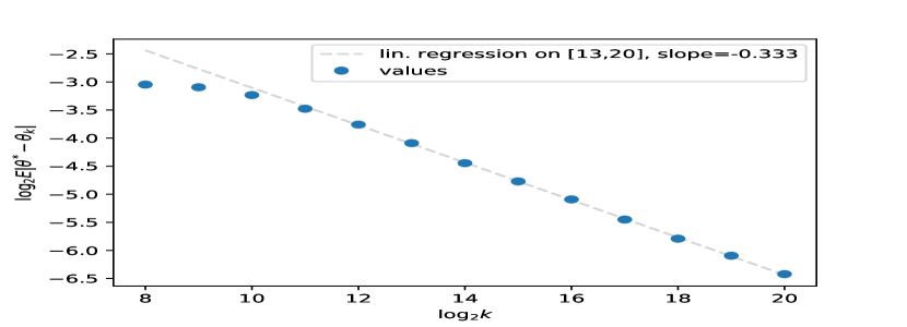
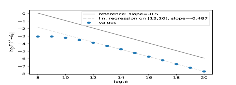
To compute the expected error, Monte Carlo simulations were used with $10000$ sample paths and the number of steps $k$ ranging from $2^{8}$ to $2^{20}$. We fit regression on the log-log plot to get the convergence rate only on $[2^{13},2^{20}]$ and set $k_{0}=10000$ to avoid the initial fluctuations of the algorithm.

5.1 Independent innovations

In this section we assume that the consecutive “measurement noises” $X_{n}$ are i.i.d. We consider three different choices for the distribution of the noise: normal, uniform and beta distributions. Note that normal distribution violates boundedness and for uniform distribution the differentiability of $F$ fails, however convergence is achieved even in these cases. We also distinguish between the case where the observations $X_{k+1}$ and $X^{\prime}_{k+1}$ are the same and when they are independent. Here we refer back to Remark 2.1 where we point out that this choice does not influence our theoretical results, however it may make a visible difference numerically. This phenomenon has already been observed, see [12] for more about the variance reduction technique called common random numbers (CRN). The values in Table 1 below represent the slope of linear regression we fit on the log-log plot of the average absolute error vs. the number of steps, together with the R-squared value measuring the goodness of the fit.

	independent $X_{k+1}$,$X^{\prime}_{k+1}$	identical $X_{k+1}=X^{\prime}_{k+1}$
N$(0,1)$	$-0.299$ $(R^{2}=0.999)$	$-0.459$ $(R^{2}=0.999)$
U$([0,1])$	$-0.14$ $(R^{2}=0.997)$	$-0.14$ $(R^{2}=0.997)$
Beta$(2,2)$	$-0.374$ $(R^{2}=0.999)$	$-0.393$ $(R^{2}=0.999)$

Table 1: Convergence speed for different distributions of i.i.d. noise

The lower limit that we theoretically achieved for the convergence rate in Theorem 2.1 was ${-0.2}$, however the numerical experiments we present show that the practical convergence rate can outperform this.

5.1.1 Standard normal distribution

Assume that $X\sim N(0,1)$. Then the function we aim to find the minimum of is $U_{1}(\theta)=1+\theta^{2}+\Phi(\theta),$ where $\Phi$ denotes the the cumulative distribution function of standard normal distribution. We get the solution $\theta^{*}=-\sqrt{W\left(\frac{1}{8\pi}\right)}\approx-0.19569,$ where $W$ is the Lambert-W function.

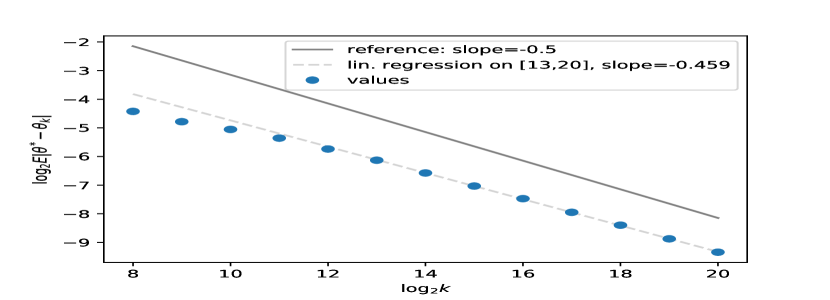
Figure 1 illustrates the convergence of two variations of algorithm (20) for $U_{1}$, starting the iteration from $\theta_{0}=-0.1$. On figure (1(a)) we present the case where $X_{k+1}$ and $X^{\prime}_{k+1}$ are independent on a log-log plot, we observe a convergence rate of $k^{-0.299}$ while (1(b)) shows the case where $X_{k+1}=X^{\prime}_{k+1}$ which yields a convergence rate of $k^{-0.459}$.

(a) $X_{k+1}$ and $X^{\prime}_{k+1}$ independent

(b) $X_{k+1}=X^{\prime}_{k+1}$

Figure 1: Log-log plot of $\mathbb{E}|\theta^{*}-\theta_{k}|$ vs. number of iterations for i.i.d. standard normal innovations

5.1.2 Uniform([0,1]) distribution

Let $X\sim Uniform([0,1])$. Then the function we aim to find the minimum of is $U_{2}(\theta)=1/3-\theta+\theta^{2}+F_{uni}(\theta),$ where $F_{uni}$ denotes the the cumulative distribution function of Uniform([0,1]) distribution. We get the solution $\theta^{*}=0.$

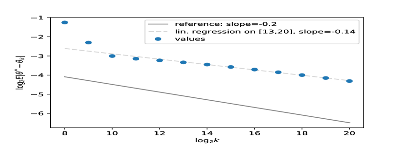
Figure 2 illustrates the convergence of two variations of algorithm (20) for $U_{2}$, starting the iteration from $\theta_{0}=1$. On figure (2(a)) we present the case where $X_{k+1}$ and $X^{\prime}_{k+1}$ are independent on a log-log plot, while (2(b)) shows the case where $X_{k+1}=X^{\prime}_{k+1}$, both of which yield a convergence rate of $k^{-0.14}$, worse that the theoretical rate $k^{-0.2}$.

(a) $X_{k+1}$ and $X^{\prime}_{k+1}$ independent

(b) $X_{k+1}=X^{\prime}_{k+1}$

Figure 2: Log-log plot of $\mathbb{E}|\theta^{*}-\theta_{k}|$ vs. number of iterations for i.i.d. uniform innovations

5.1.3 Beta(2,2) distribution

Let $X\sim Beta(2,2)$. Then the function we aim to find the minimum of is $U_{3}(\theta)=0.3-\theta+\theta^{2}+F_{\beta}(\theta),$ where $F_{\beta}$ denotes the the cumulative distribution function of Beta(2,2) distribution. We get the solution $\theta^{*}=\frac{2-\sqrt{2.5}}{3}\approx 0.13962.$

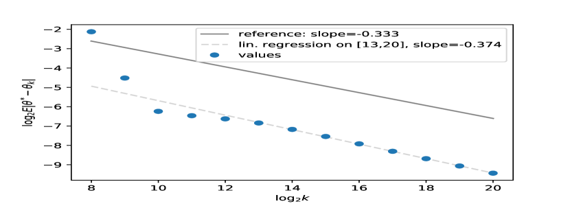
Figure 3 illustrates the convergence of two variations of algorithm (20) for $U_{3}$, starting the iteration from $\theta_{0}=1$. On figure (3(a)) we present the case where $X_{k+1}$ and $X^{\prime}_{k+1}$ are independent on a log-log plot, we observe a convergence rate of $k^{-0.374}$ while (3(b)) shows the case where $X_{k+1}=X^{\prime}_{k+1}$ which yields a convergence rate of $k^{-0.393}$.

(a) $X_{k+1}$ and $X^{\prime}_{k+1}$ independent

(b) $X_{k+1}=X^{\prime}_{k+1}$

Figure 3: Log-log plot of $\mathbb{E}|\theta^{*}-\theta_{k}|$ vs. number of iterations for i.i.d. beta innovations

5.2 AR(1) innovations

For an example with non-i.i.d. $X_{t}$, assume that the “noise” is an AR(1) process defined as

$$Y_{t+1}=\kappa Y_{t}+\varepsilon_{t+1}\text{, for }t\in\mathbb{Z},$$

where $\varepsilon_{t}$ is standard normal for $t\in\mathbb{Z}$ and $|\kappa|<1$. Clearly, $Y_{t}=\sum_{k=0}^{\infty}\kappa^{k}\varepsilon_{t-k},$ and therefore $Y_{t}\sim N\left(0,\frac{1}{1-\kappa^{2}}\right)$. For the sequences $X_{t}$ and $X_{t}^{\prime}$ we have two options: either we take consecutive measurements i.e. $X_{k}=Y_{2k-1}$ and $X^{\prime}_{k}=Y_{2k}$ or we use identical values, i.e. $X_{k}=X^{\prime}_{k}=Y_{k}$. In both cases

$$U_{4}(\theta)=\mathbb{E}J(\theta,X)=\theta^{2}+\frac{1}{1-\kappa^{2}}+\Phi\left(\theta\sqrt{1-\kappa^{2}}\right).$$

Solving this for $\kappa=0.75$ we get the optimal value $\theta^{*}\approx-0.13144.$

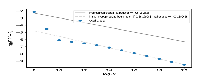
Figure 4 and table 2 illustrate the convergence rate of algorithm (20) for the function $U_{4}$, starting from $\theta_{0}=0$. On figure (4(a)) we present the rate in the case where we take consecutive measurements of the AR(1) process, ($X_{k}=Y_{2k-1}$ and $X^{\prime}_{k}=Y_{2k}$), the convergence rate of $k^{-0.333}$ was observed. Figure (4(b)) shows the case where the two measurements are the same, ($X_{k}=X^{\prime}_{k}=Y_{k}$), with the rate $k^{-0.487}$.

	consecutive observations: $X_{k}=Y_{2k-1}$ and $X^{\prime}_{k}=Y_{2k}$	identical: $X_{k}=X^{\prime}_{k}=Y_{k}$
AR(1)	-0.333 $(R^{2}=0.999)$	-0.487 $(R^{2}=0.999)$

Table 2: Convergence rate for AR(1) noise

(a) $X_{k}=Y_{2k-1}$ and $X^{\prime}_{k}=Y_{2k}$

(b) $X_{k}=X^{\prime}_{k}=Y_{k}$

Figure 4: Log-log plot of $\mathbb{E}|\theta^{*}-\theta_{k}|$ vs. number of iterations for AR(1) innovations

6 Application to mathematical finance

The price of a financial asset either follows a trend during a given period of time or just rambles around its “fair” price value – at least so it seems to many actual traders. This “rambling”, in more mathematical terms, means that the price is reverting to its long-term average. Such a mean-reversion phenomenon can be exploited by “buying low, selling high”-type strategies. Related discussions involve plenty of common-sense advice and benevolent concrete suggestion, see e.g. [21, 22, 23]. There exist also theoretical studies about optimal trading with such prices, see e.g. [13]. However, a rigorous approach to adaptive trading algorithms of this type is lacking.

Results of the present paper provide theoretical convergence guarantees for such algorithms which cannot be deduced from existing literature on stochastic approximation. The most conspicuous feature of mean-reversion strategies is that they are triggered when the price reaches a certain level. This means that their payoffs are discontinuous with respect to the parameters, gradients do not exist and only finite-difference approximations can be used (the Kiefer-Wolfowitz method). Their convergence in the given discontinuous case cannot be shown based on available results hence we fill an important and practically relevant gap here.

We describe in some detail a trading model below and explain how it fits into the framework used in the previous sections. Let the price of the observed financial asset be described by a real-valued stochastic process $S_{t}$, $t\in\mathbb{Z}$, adapted to a given filtration $\mathcal{F}_{t}$, $t\in\mathbb{Z}$, representing the flow of information. (Alternatively $S_{t}$ may be the increment of the price at $t$ which can safely be assumed to follow a stationary process.)

Our algorithm will be based on several dynamically updated estimators which are assumed to be functionals of the trajectories of $S_{t}$ and possibly of another adapted process $F_{t}$ describing important economic factors. The estimate for the long-term average of the process is denoted by $A_{t}(\theta)$ at time $t$. The upper and lower bandwith processes will be denoted $B_{t}^{+}(\theta)$ and $B_{t}^{-}(\theta)$, they are non-negative. All these estimates depend on a parameter $\theta$ to be tuned, where $\theta$ ranges over a subset $Q$ of $\mathbb{R}^{d}$.

In practice, $A_{t}(\theta)$ is some moving average (or exponential moving average) of previous values of $S$ but it may depend on the other indicators $F$ (market indices, etc.). Here $\theta$ determines, for instance, the weights of the moving average estimate. The quantities $B_{t}^{\pm}(\theta)$ are normally based on standard deviation estimates for $S$ but, again, may be more complex with $\theta$ describing weighting of past information. If we peek from time $t$ back to time $t-p$ with some $p\in\mathbb{N}$ then $A_{t}(\theta),B^{\pm}_{t}(\theta)$ are functionals of $(S_{t-p},F_{t-p},\ldots,S_{t},F_{t})$.

The price range $[A_{t}-B^{-}_{t},A_{t}+B^{+}_{t}]$ is considered to be “normal” by the algorithm while quitting that interval suggest “extremal” behaviour that the market should correct soon. For example, reaching the level $A_{t}-B^{-}_{t}$ means that the price is abnormally low for the present circumstances, hence it is worth buying a quantity $b(\theta)$ of them where, again, the parameter $\theta$ should be optimally found. When the price returns to $A_{t^{\prime}}$ at some later time $t^{\prime}$, the asset will be sold and a profit is realized. Similarly, when reaching $A_{t}+B^{+}_{t}$, quantity $s(\theta)$ of the asset is sold (the price being abnormally high) and it will be repurchased once the “normal” level $A_{t^{\prime}}$ is reached at some future $t^{\prime}>t$, aiming to realize profit.

The value of the parameter $\theta$ will be updated at times $tN$, $t\in\mathbb{N}$ where $N\geq 1$ is fixed. The (random) profit (or loss) resulting from trading on the interval $[N(t-1),Nt]$ is denoted by $u(\theta,X_{t})$ with $X_{t}=(S_{N(t-1)-p},F_{N(t-1)-p},\ldots,S_{Nt},F_{Nt})$. We could even write an explicit expression for $u$ based on the description of the trading mechanism in the previous paragraph but it would be very cumbersome without providing additional insight hence we omit it. We also add that, in many cases, a fee must also be paid at every transaction. Such strategies being “threshold-type”, the function $u$ is generically a discontinuous function of $\theta$.

We furthermore argue that one cannot smooth out $u$ and make it continuous without losing essential features of the problem. Approximating the indicator function of the interval $[0,\infty)$ by a function $f$ which is $1$ on $[0,\infty)$, $0$ on $(-\infty,-\epsilon]$ for some small $\epsilon>0$ and linear on $(-\epsilon,0)$ may look reasonable at first sight but in this way we get a Lipschitz approximation with a huge Lipschitz constant hence with a poor convergence rate! This is just to stress that such simple tricks might work in certain practical situations but they only obscure the real issues in the theoretical analysis (namely, there is a discontinuity to be handled).

The described algorithm is very close to what actual investors do, see [21, 22, 23]. We also mention the related theoretical studies [18, 3] which, however, do not take an adaptive view and calculate optimal strategies for concrete models.

Taking a more realistic, adaptive approach, the investor may seek to maximize $Eu(\theta,X_{0})$ by dynamically updating $\theta$ at every instant $tN$, $t\in\mathbb{N}$. Our versions of the Kiefer-Wolfowitz algorithm, presented in the previous sections, are tailor-made for such online optimization, both the decreasing and the fixed gain version, depending on the circumstances. Theorems 2.1 and 2.2 provide solid theoretical convergence guarantees for such procedures.

References

- [1] M. Barkhagen, N. H. Chau, É. Moulines, M. Rásonyi, S. Sabanis, and Y. Zhang. On stochastic gradient Langevin dynamics with dependent data streams in the logconcave case. Bernoulli, 27:1–33, 2021.
- [2] A. Benveniste, M. Métivier, and P. Priouret. Adaptive algorithms and stochastic approximations. Springer, 1990.
- [3] Á. Cartea, S. Jaimungal and J. Penalva. Algorithmic and high-frequency trading. Cambridge University Press, 2015.
- [4] H. N Chau, C. Kumar, M. Rásonyi, and S. Sabanis. On fixed gain recursive estimators with discontinuity in the parameters. ESAIM: Probability and Statistics, 23:217–244, 2019.
- [5] N. H. Chau, É. Moulines, M. Rásonyi, S. Sabanis, and Y. Zhang. On stochastic gradient Langevin dynamics with dependent data streams: the fully non-convex case. To appear in SIAM Journal on Mathematics of Data Science, 2021. arXiv:1905.13142
- [6] A. Durmus and É. Moulines. Nonasymptotic convergence analysis for the unadjusted Langevin algorithm. Annals of Applied Probability, 27:1551–1587, 2017.
- [7] G. Fort, É. Moulines, A. Schreck, and M. Vihola. Convergence of Markovian stochastic approximation with discontinuous dynamics. SIAM Journal on Control and Optimization, 54(2):866–893, 2016.
- [8] L. Gerencsér. On a class of mixing processes. Stochastics, 26(3):165–191, 1989.
- [9] L. Gerencsér. Rate of convergence of recursive estimators. SIAM Journal on Control and Optimization, 30(5):1200–1227, 1992.
- [10] L. Gerencsér. Convergence rate of moments in stochastic approximation with simultaneous perturbation gradient approximation and resetting. IEEE Trans. Automatic Control, 44:894–905, 1999.
- [11] L. Gerencsér. SPSA with state-dependent noise. A tool for direct adaptive control. In: Proc. of the 37th IEEE Conference on Decision and Control, Tampa, Fl., USA, (IEEE, 1998), 3451–3456, 1998.
- [12] P. Glasserman and D. D. Yao. Some guidelines and guarantees for common random numbers. Management Science, 38(6):884–908, 1992.
- [13] P. Guasoni, A. Tolomeo and G. Wang. Should Commodity Investors Follow Commodities’ Prices? SIAM Journal on Financial Mathematics, 10:466–490, 2019.
- [14] J. Kiefer and J. Wolfowitz. Stochastic estimation of the maximum of a regression function. Annals of Mathematical Statistics, 23(3):462–466, 1952.
- [15] H. J. Kushner and D. S. Clark. Stochastic approximation for constrained and unconstrained systems. Springer, 1978.
- [16] S. Laruelle and G. Pagès. Stochastic approximation with averaging innovation applied to finance. Monte Carlo Methods and Applications, 18(1):1–51, 2012.
- [17] L. Ljung. Analysis of recursive stochastic algorithms. IEEE Transactions on Automatic Control, 22(4):551–575, 1977.
- [18] T. Leung and X. Li. Optimal Mean Reversion Trading. World Scientific, 2015.
- [19] H. Robbins and S. Monro. A stochastic approximation method. Annals of Mathematical Statistics, 22(3):400–407, 1951.
- [20] J. Sacks. Asymptotic distribution of stochastic approximation procedures. Annals of Mathematical Statistics, 29:373–405, 1958.
- [21] https://tradergav.com/what-is-mean-reversion-trading-strategy/
- [22] https://www.warriortrading.com/mean-reversion/
- [23] https://tradingstrategyguides.com/mean-reversion-trading-strategy/