Two-size Probability-Changing Cluster Algorithm

Abstract

We propose a self-adapted Monte Carlo approach to automatically determine the critical temperature by simulating two systems with different sizes at the same temperature. The temperature is increased or decreased by checking the short-time average of the correlation ratios of the two system sizes. The critical temperature is achieved using the negative feedback mechanism, and the thermal average near the critical temperature can be calculated precisely. The proposed approach is a general method to treat second-order phase transition, first-order phase transition, and Berezinskii-Kosterlitz-Thouless transition on the equal footing.

1 Introduction

Finite-size scaling (FSS) [1] is a basic concept in the study of phase transitions and critical phenomena. The Binder ratio [2], essentially the moment ratio, is widely used in the analysis of the numerical data. The moment ratios of the magnetization $m$,

$$U(T)=\langle m(T)^{4}\rangle/\langle m(T)^{2}\rangle^{2},$$ (1)

for different sizes scale as

$$U(T)=f(tL^{1/\nu}),$$ (2)

where $t=(T-T_{c})/T_{c}$ and $\nu$ is the correlation-length exponent. The linear system size is denoted by $L$. We can determine the critical temperature $T_{c}$ of the second-order phase transition by employing a condition where $U(T)$ does not depend on $L$. By measuring $U(T)$ for different sizes, we can determine $T_{c}$ from the crossing point of temperature-dependent curves of different sizes. We note that there are corrections to FSS. There are other quantities that satisfy the scaling form such as Eq. (2); the second-moment correlation length divided by $L$ [3] and the ratio of the correlation functions with different distances [4] are examples of such quantities.

Moreover, if we consider the ratio of $U(T)$ with different sizes, e.g., $U(T,L)/U(T,L/2)$, the critical value of this ratio becomes one, even if the critical value of $U(T)$ itself is not a universal one, and does depend on the model. The ratios of $U(T)$ with different sizes were studied in the analysis of the Potts model [5, 6]. These ratios were also used in the recent analysis of the clock model [7].

The FSS analysis is often associated with the Monte Carlo simulation. To overcome the slow dynamics in the single-spin flip algorithm, a multi-cluster flip algorithm was proposed by Swendsen and Wang [8]. Wolff [9] proposed another type of cluster algorithm, that is, a single-cluster flip algorithm. Tomita and Okabe [10] developed a cluster algorithm, called the probability-changing cluster (PCC) algorithm, for automatically determining the critical point. It is an extension of the cluster algorithm, but it changes the probability of cluster update (essentially, the temperature) during the Monte Carlo process.

This paper presents a self-adapted method using two system sizes for automatically determining the critical temperature, which is referred to as the two-size PCC algorithm. We simultaneously perform the Monte Carlo simulations for the two system sizes. We measure some quantity $U$, which follows the scaling form shown in Eq. (2), and calculate the ratio of $U(L)/U(L/2)$ for short time. Then, we increase or decrease the temperature by checking the value of $U(L)/U(L/2)$.

We start with the two-size PCC algorithm for the second-order transition. As an example, we treat the two-dimensional (2D) Ising model, and demonstrate how the critical temperature can be determined in a self-adapted way. We calculate the thermal average of the physical quantities near the critical temperature. We also study the first-order transition. As a typical example, we deal with the 2D 6-state Potts model. We investigate the first-order transition temperature and the latent heat. We demonstrate that the same procedure is also effective for studying the Berezinskii-Kosterlitz-Thouless (BKT) transition, where a fixed line instead of a fixed point exists. We select the 2D 5-state clock model that has two BKT transitions with higher and lower transition temperatures.

The remaining part of the paper is organized as follows: We describe the two-size PCC algorithm for the second-order transition in Section II. Two-size PCC studies of the first-order transition and BKT transition are discussed in Sections III and IV, respectively. Section V is devoted to summarizing the study and discussing results.

2 Second-order transition

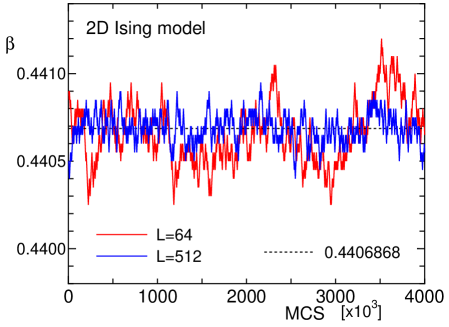
Figure 1: The time evolution of $\beta$ with the two-size PCC algorithm for the 2D Ising model. The system sizes are $L=64$ and $L=512$; that is, the set of system sizes are (64,32) and (512,256). The exact value of $\beta_{c}$ (=$\ln(1+\sqrt{2})/2=0.4406868$) for an infinite system is denoted by a dotted line.

Let us start with the second-order phase transition. As an example, we consider a 2D Ising model on the square lattice, whose Hamiltonian is given by

$$H=-J\sum_{\langle ij\rangle}\sigma_{i}\sigma_{j},\quad\sigma_{i}=\pm 1.$$ (3)

The summation is taken over the nearest-neighbor pairs, and periodic boundary conditions are imposed in numerical simulations. Using the Wolff single-cluster flip algorithm for spin update, we simulate the two system sizes simultaneously. In determining the critical point (line), we use the ratio of the correlation functions with different distances, i.e., the correlation ratio [4],

$$R(T)=\langle g(r)\rangle/\langle g(r^{\prime})\rangle.$$ (4)

Here, $g(r)$ is a correlation function with the distance $r$. For the values of $r$ and $r^{\prime}$, we choose $r=L/2$ and $r^{\prime}=L/4$ for numerical calculations.

The actual procedure for the two-size PCC algorithm is as follows. We use two systems of different sizes, say $L$ and $L/2$. After simulating some steps at the same temperature, we measure the correlation ratios of both the systems, $R(L)$ and $R(L/2)$. We increase or decrease the inverse temperature $\beta$ (= $1/T$ in units of the coupling $J$) according to the following rule:

$$\beta=\left\{\begin{array}[]{ll}\beta+\Delta\beta&\quad\mbox{if $R(L)/R(L/2)<1$},\\ \beta-\Delta\beta&\quad\mbox{otherwise},\end{array}\right.$$ (7)

where $\Delta\beta>0$. There are two parameters to choose, the number of Monte Carlo steps (MCS) for taking a short-time average, $N_{\rm av}$, and the difference of $\beta$, $\Delta\beta$. Note that the cluster flip algorithm is effective because the rapid equilibration is required after a change in temperature.

The plot of the time evolution of $\beta$ is shown in Fig. 1. For this plot, we chose $N_{\rm av}$ = 4000 and $\Delta\beta$ = 0.00005; that is, after every 4000 MCS, $\beta$ is changed by $\pm 0.00005$. We will discuss the choice of $N_{\rm av}$ and $\Delta\beta$ later. In the figure, the time steps are given in units of 1000 MCS, and we show the data up to $4\times 10^{6}$ MCS. The system sizes are $L=64$ and $L=512$; that is, the set of system sizes are (64,32) and (512,256). We see that the temperature oscillates around the average value. The width of fluctuation decreases as the system size increases because of the effect of self-averaging. For convenience, we denote the exact value of $\beta_{c}$ (=$\ln(1+\sqrt{2})/2=0.4406868$) for an infinite system by a dotted line.

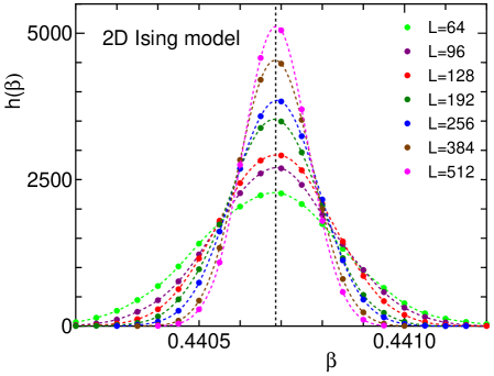
Figure 2: The size dependence of the histogram of $\beta$, $h(\beta)$, for the 2D Ising model. The system sizes are $L$ = 64, 96, 128, 192, 256, 384, and 512; the condition for averaging is $N_{\rm av}$=4000, $\Delta\beta$=0.00005. The exact value of $\beta_{c}$ (=$\ln(1+\sqrt{2})/2=0.4406868$) for an infinite system is denoted by a dotted line.

Next, we examine the histogram of $\beta$, $h(\beta)$, for the two-size PCC algorithm. We plot $h(\beta)$ of the 2D Ising model for $L$ = 64, 96, 128, 192, 256, 384, and 512 in Fig. 2. Measurement is performed for $4\times 10^{6}$ MCS after equilibration of 10,000 MCS. We made 32 runs for each system size in order to estimate statistical errors. For smaller sizes ($L$ = 64, 96, and 128), we made 64 runs. The parameters $N_{\rm av}$ and $\Delta\beta$ were chosen as 4000 and 0.00005, respectively. In the plot, the histogram $h(\beta)$ is normalized by

$$\int h(\beta)\ d\beta=1.$$

The obtained histogram is similar to normal distribution, and we see that the histogram becomes sharper with an increase in system size. Furthermore, the peak position approaches the exact value of $\beta_{c}$ for the infinite system.

Here, we examine the choice of $N_{\rm av}$ and $\Delta\beta$. Figure 3 shows a comparison of $h(\beta)$ of the 2D Ising model with $L=128$ for five conditions; (a) $N_{\rm av}$=4000, $\Delta\beta$=0.00005, (b) $N_{\rm av}$=4000, $\Delta\beta$=0.000025, (c) $N_{\rm av}$=4000, $\Delta\beta$=0.0001, (d) $N_{\rm av}$=2000, $\Delta\beta$=0.00005, (e) $N_{\rm av}$=8000, $\Delta\beta$=0.00005. The histogram becomes sharper with a decrease in $\Delta\beta$ and an increase in $N_{\rm av}$. The systematic size dependence is obtained when the conditions of $N_{\rm av}$ and $\Delta\beta$ are fixed. In the following, we will show the data for condition (a) $N_{\rm av}$=4000, $\Delta\beta$=0.00005.

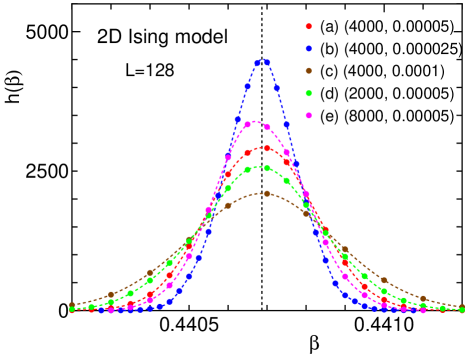
Figure 3: The comparison of the histogram of $\beta$, $h(\beta)$, for the 2D Ising model. The system sizes is set to be $L$ = 128, and the conditions for averaging are (a) $N_{\rm av}$=4000, $\Delta\beta$=0.00005, (b) $N_{\rm av}$=4000, $\Delta\beta$=0.000025, (c) $N_{\rm av}$=4000, $\Delta\beta$=0.0001, (d) $N_{\rm av}$=2000, $\Delta\beta$=0.00005, (e) $N_{\rm av}$=8000, $\Delta\beta$=0.00005.

The transition (inverse) temperature for each size, $\beta_{c}(L)$, was estimated using the averaged value of $\beta$. The plot of the size dependence of $\beta_{c}(L)$ as a function of $1/L$ is shown in Fig. 4, where the statistical errors were estimated by $2\sigma$ of the distribution of $\beta_{c}$. We can see from Fig. 4 that $\beta_{c}(L)$ rapidly approaches the exact value $\ln(1+\sqrt{2})/2=0.4406868$, which is denoted by a dotted line, even for small sizes. The rapid convergence of the present algorithm is apparent when we compare the size-convergence rate of $\beta_{c}(L)$ with that of the original PCC (Fig. 1 of Ref. [10]). In the original version of the PCC algorithm, although the size-dependent $\beta_{c}(L)$ is automatically tuned, we still have to consider the size dependence of $\beta_{c}(L)$ based on the FSS. Instead, with the two-size PCC algorithm, the infinite-size critical temperature is easily achieved even for small sizes.

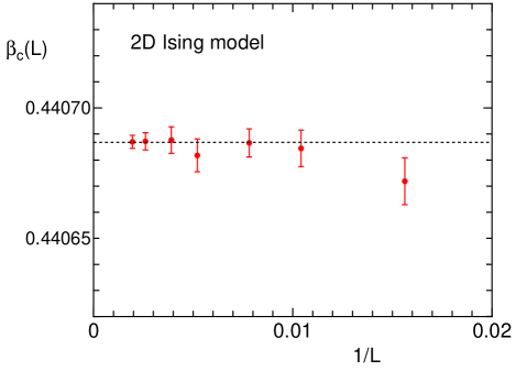
Figure 4: The plot of $\beta_{c}(L)$ of the 2D Ising model. The linear system sizes $L$ are 64, 96, 128, 192, 256, 384, and 512. The exact value is denoted by a dotted line.

The energy distribution $p(E/N)$ is plotted in Fig. 5 for $L$ = 64, 96, 128, 192, 256, 384, and 512. The energy distribution is normalized by

$$\int p(E/N)\ d(E/N)=1.$$

There is a single peak, which will be compared with the case of the first-order transition later. We see that the distribution becomes sharper as the system size increases. The peak position approaches the exact energy at the critical temperature, that is, $E/N$ = $-\sqrt{2}=-1.41421$. The exact critical value is denoted by a dotted line in the figure.

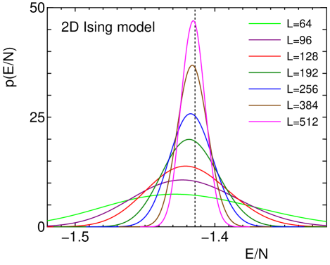
Figure 5: The plot of $p(E/N)$ for the 2D Ising model. The system sizes are $L$ = 64, 96, 128, 192, 256, 384, and 512; the condition for averaging is $N_{\rm av}$=4000, $\Delta\beta$=0.00005.

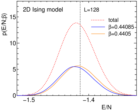
Figure 6: The plot of the $\beta$-decomposed energy distribution $p(E/N;\beta)$ for the 2D Ising model. The system size is $L=128$. The data of two $\beta$’s are compared. The whole distribution $p(E/N)$ is shown by a dotted line.

Because each system wanders around temperature, we can take a thermal average of physical quantities at each temperature. This is the same situation encountered in the replica exchange method [11]. There, the temperatures of replicas are exchanged following the transition probabilities based on the Boltzmann weight; the thermal average at a fixed $\beta$ is obtained by averaging over different replicas. Before showing the data of the thermal average of physical quantities, we present the energy distribution for a fixed value of $\beta$. The energy distribution is decomposed as

$$p(E)=\sum_{\beta}p(E;\beta).$$ (8)

The data of $p(E/N;\beta)$ at two typical temperatures, $\beta$ = 0.44085 and 0.4405, together with the whole distribution of $p(E/N)$, is shown in Fig. 6. The system size is fixed at $L=128$. The value of the $\beta$-decomposed distribution is magnified twenty times for clarity. Two energy distributions with different values of $\beta$ are related to each other through the equation

$$p(E;\beta^{\prime})\propto e^{-(\beta^{\prime}-\beta)E}\ p(E;\beta).$$ (9)

It is a reweighting of the Boltzmann factor, which is the basis of the histogram method by Ferrenberg and Swendsen [12]. The thermal average of a physical quantity $A$ at $\beta^{\prime}$ is obtained by the measurement at $\beta$ through the relation

$$\langle A\rangle_{\beta^{\prime}}=\frac{[A(E)\ e^{-(\beta^{\prime}-\beta)E}]_{\beta}}{[e^{-(\beta^{\prime}-\beta)E}]_{\beta}},$$ (10)

where $[\cdots]$ stands for the Monte Carlo average at $\beta$. We note that the $\beta$-decomposed energy distribution, $p(E/N;\beta)$, does not depend on $h(\beta)$. Thus, we obtain the thermal average of a physical quantity $A$, $\langle A\rangle_{\beta}$, without considering $N_{\rm av}$ and $\Delta\beta$.

As an example of the physical quantities, we show the correlation ratio $R(\beta)$ as a function of temperature for various system sizes in Fig. 7. We see that the data of different sizes intersect at the critical point within statistical errors. The critical value of the correlation ratio, $R_{c}$, is calculated as follows:

$$\frac{\langle g(L/2)\rangle}{\langle g(L/4)\rangle} = \frac{\displaystyle|\theta_{1}(1/2)|^{-1/4}\ \sum_{\nu=1}^{4}|\theta_{\nu}(1/4)|}{\displaystyle|\theta_{1}(1/4)|^{-1/4}\ \sum_{\nu=1}^{4}|\theta_{\nu}(1/8)|}$$ (11)

$$= 0.943905,$$

using the Jacobi $\theta$-functions [13] (see also Refs. [14, 4]). This value is denoted by a dotted line in Fig. 7. Our simulation reproduces the exact value of $R_{c}$ with an accuracy up to four digits.

Now let us consider the FSS. Because the critical temperature and the critical exponents are known for the 2D Ising model, $R(\beta)$ are plotted as a function of $(\beta-\beta_{c})L^{1/\nu}$, as shown in Fig. 8, where $\beta_{c}=\ln(1+\sqrt{2})/2$ and $1/\nu=1$. We see that the FSS works quite well.

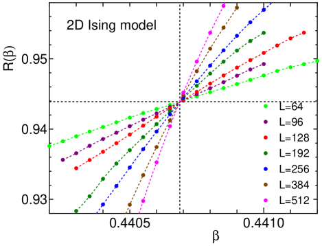
Figure 7: The plot of $R(\beta)$ for the 2D Ising model. The system sizes are $L$ = 64, 96, 128, 192, 256, 384, and 512. The exact values of $\beta_{c}$ and $R_{c}$ are given by a dotted line.

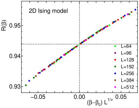
Figure 8: The FSS plot of $R(\beta)$ for the 2D Ising model. The system sizes are $L$ = 64, 96, 128, 192, 256, 384, and 512.

3 First-order phase transition

We now consider the case of the first-order phase transition. The 2D ferromagnetic $q$-state Potts model [15, 16, 17] is taken into account. The Hamiltonian is given by

$$H=J\sum_{\langle ij\rangle}(1-\delta_{s_{i}s_{j}}),\quad s_{i}=1,2,\cdots,q,$$ (12)

where $\delta_{ab}$ is the Kronecker delta. This model is known to show the second-order phase transition for $q\leq 4$ and first-order phase transition for $q\geq 5$.

Here, we provide the data for a two-size PCC calculation of the 2D 6-state Potts model. Hysteresis in the first-order transition systems should be considered, which is different from the conditions of the second-order transition. It is more feasible to employ the multi-cluster update of the Swendsen-Wang type [8] because a spin configuration changes extensively with such an update. For the systems with the second-order transition, there is no appreciable difference in the choice of the cluster update. The number of the steps for calculating the short-time average, $N_{\rm av}$, and the difference in $\beta$, $\Delta\beta$, were chosen as 4000 and 0.00001, respectively. We used smaller values of $\Delta\beta$ as this could help reduce the effect of hysteresis. We conducted measurements for $4\times 10^{6}$ steps after equilibration of 10,000 steps; such measurements were repeated 64 times for $L$ = 64 and 96, and 32 times for $L$ = 128, 192, 256, 384, and 512. We note that the correlation function of the $q$-state Potts model is given as

$$g(r)=\frac{q\sum_{i}\delta_{s_{i}s_{i+r}}-N}{q-1}.$$ (13)

The histogram of $\beta$, $h(\beta)$, for the system sizes $L$ = 64, 96, 128, 192, 256, 384, and 512 is shown in Fig. 9. The histogram exhibits sharp peaks, and the peak position gradually approaches the exact value. The exact value of the first-order transition inverse temperature for the infinite system is given by $\ln(1+\sqrt{q})$ = 1.23823 (for $q=6$), in units of $J$, which is shown by the dotted line.

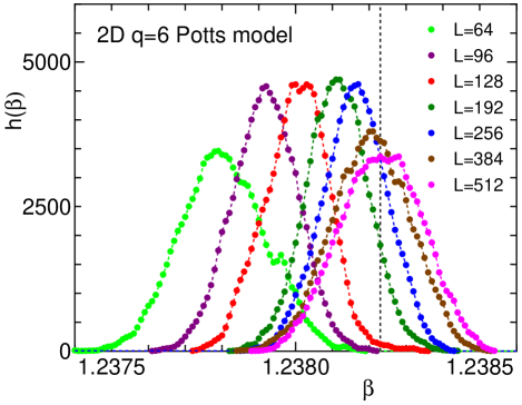
Figure 9: The plot of $h(\beta)$ for the 2D $q=6$ Potts model. The system sizes are $L$ = 64, 96, 128, 192, 256, 384, and 512; the condition for averaging is $\Delta\beta$=0.00001, $N_{\rm av}$=4000. The exact value of $\beta_{c}$ (=$\ln(1+\sqrt{6})=1.23823$) for the infinite system is given by a dotted line.

The average value of $\beta$, $\beta_{c}(L)$, is plotted as a function of $1/L$ in Fig. 10. The exact value of the first-order transition inverse temperature (1.23823) is given by the dotted line. We can observe that the calculated estimate of the transition temperature converges to the exact value with five-digit accuracy.

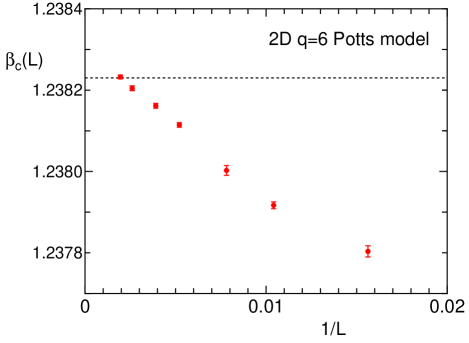
Figure 10: The plot of $\beta_{c}(L)$ of the 2D $q=6$ Potts model. The linear system sizes $L$ are 64, 96, 128, 192, 256, 384, and 512. The exact value is denoted by a dotted line.

The distribution of $E$, $p(E/N)$, is shown in Fig. 11 for various sizes. We observe double peaks, which are specific to the first-order transition. In Fig. 12, we plot the $\beta$-decomposed energy distribution, $p(E/N;\beta)$. The system size is set to be $L=128$. Here, we show the data of two typical temperatures, $\beta$ = 1.23809 and 1.23794, which are on both sides of the peak value of $h(\beta)$ shown in Fig. 9, together with the entire distribution of $p(E/N)$. The value of the $\beta$-decomposed distribution is magnified twenty times for clarity. We can observe that the weight of high energies increases for the high-temperature (low-$\beta$) energy distribution.

We now examine the peak positions of energy. Baxter [18] (see also [19]) calculated the exact difference in the higher energy peak $E_{2}$ and the lower energy peak $E_{1}$, i.e., the latent heat. The exact result is

$$(E_{2}-E_{1})/N=2(1+\frac{1}{\sqrt{q}})\tanh\frac{\Theta}{2}\prod_{n=1}^{\infty}(\tanh n\Theta)^{2},$$ (14)

where $\Theta=\textrm{arcosh}(\sqrt{q}/2)$. The middle point $(E_{1}+E_{2})/2N$ is also given as

$$(E_{1}+E_{2})/2N=1-1/\sqrt{q}.$$ (15)

Thus, for $q=6$, $E_{1}/N$ and $E_{2}/N$ are calculated as 0.49102 and 0.69248, respectively. These values are given in Fig. 11. We can observe that the positions of the energy peaks approach the exact infinite values as the system size increases. The size dependences of the numerical estimates of $E_{1}/N$ and $E_{2}/N$ are plotted as a function of $1/L$ in Fig. 13. The statistical errors are within the size of marks. They converge to the exact values [18].

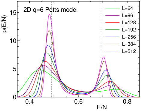
Figure 11: The plot of $p(E/N)$ for the 2D $q=6$ Potts model. The system sizes are $L$ = 64, 96, 128, 192, 256, 384, and 512. Baxter’s results [18] for two peak positions are given by dotted lines.

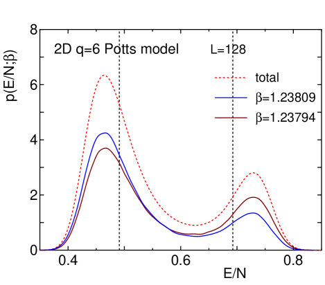
Figure 12: The plot of the $\beta$-decomposed energy distribution $p(E/N;\beta)$ for the 2D $q=6$ Potts model. The system size is $L=128$. The data of two $\beta$’s are compared. The whole distribution $p(E/N)$ is shown by a dotted line.

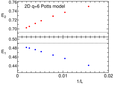
Figure 13: The plot of $E_{1}$ and $E_{2}$ as a function of $1/L$ for the 2D $q=6$ Potts model. The system sizes are $L$=64, 96, 128, 192, 256, 384, and 512. Baxter’s results [18] for two peak positions are given by dotted lines.

4 BKT transition

The 2D spin systems with continuous XY symmetry exhibit a unique phase transition called the Berezinskii-Kosterlitz-Thouless (BKT) transition [20, 21, 22]. There exists a BKT phase of a quasi long-range order (QLRO), where the correlation function decays as a power law. Here, we consider the $q$-state clock model, which is a discrete version of the classical XY model. The Hamiltonian is given by

$$H=-J\sum_{\langle ij\rangle}\cos(\theta_{i}-\theta_{j}),\quad\theta_{i}=2\pi i/q,\ i=1,2,\cdots,q.$$ (16)

The 2D $q$-state clock model experiences the BKT transition for $q\geq 5$, whereas the $q=4$ clock model is two sets of the Ising model and the 3-state clock model is equivalent to the 3-state Potts model. The $q=2$ clock model is simply the Ising model.

For $q\geq 5$, there is an interplay between the plane-rotator symmetry, which attempts to preserve the BKT phase, and the discreteness, which tends to create a long-range order (LRO) at low temperatures. Two transition temperatures, $T_{1}<T_{2}$, are observed; each corresponds to the transition between LRO and QLRO and between QLRO and a disordered phase.

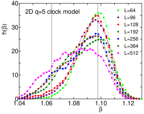
Figure 14: The plot of $h(\beta)$ for the 2D $q=5$ clock model. The system sizes are $L$ = 64, 96, 128, 192, 256, 384, and 512. The numerical estimates of $\beta_{1}$ and $\beta_{2}$ are given by dotted lines.

We conducted a simulation of the two-size PCC algorithm for the 2D $q=5$ clock model. As the system has a wide temperature range in the critical state, we selected a larger $\Delta\beta$, 0.002. Again, we selected $N_{\rm av}$=4000. A histogram of $\beta$, $h(\beta)$, of the $q=5$ clock model is shown in Fig. 14. The data in the histogram are widely distributed, which is contrast to the case of strong transitions, i.e., the second-order and first-order transitions. This is related to the fact that there is a fixed line instead of a fixed point for the system with the BKT transition. In the figure, the numerical estimates of $\beta_{1}$ ($1/T_{1}=1/0.911(5)$) and $\beta_{2}$ ($1/T_{2}=1/0.940(5)$) [7] are shown by dotted lines for convenience.

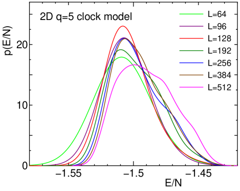
Figure 15: The plot of $p(E)$ for the 2D $q=5$ clock model. The system sizes are $L$ = 64, 96, 128, 192, 256, 384, and 512.

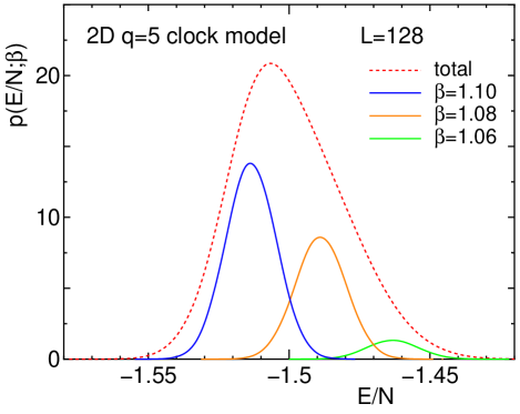
Figure 16: The plot of the $\beta$-decomposed energy distribution $p(E/N;\beta)$ for the 2D $q=5$ clock model. The system size is $L=128$. We show the data for three $\beta$’s; from left, $\beta$=1.10, 1.08, and 1.06. The whole distribution $p(E/N)$ is shown by a dotted line.

The distribution of $E$, $p(E/N)$, is shown in Fig. 15 for various sizes. In Fig. 16, we plot the $\beta$-decomposed energy distribution $p(E/N;\beta)$. The system size is $L=128$. Data for three $\beta$’s are shown; from left, $\beta$=1.10, 1.08, and 1.06. The value of the $\beta$-decomposed distribution is magnified ten times for clarity. Energy peaks are observed at certain values depending on the temperature.

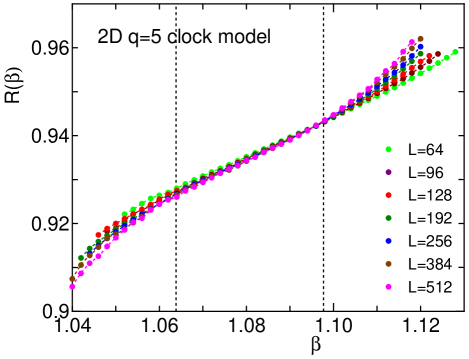
Figure 17: The plot of $R(\beta)$ for the 2D $q=5$ clock model. The system sizes are $L$ = 64, 96, 128, 192, 256, 384, and 512. The numerical estimates of $\beta_{1}$ and $\beta_{2}$ are given by dotted lines.

We calculate the temperature dependence of physical quantities using the same procedure as the one followed by the Ising model. Although the histogram $h(\beta)$ shown in Fig. 14 is not very smooth, fairly accurate estimates of the thermal average of physical quantities at a fixed $\beta$ can be obtained as was discussed in the case of the Ising model. The temperature dependence of the correlation ratio for various sizes is plotted in Fig. 17. The numerical estimates of $\beta_{1}$ and $\beta_{2}$ reported in [7] are shown by dotted lines for convenience. In the intermediate temperature range, the correlation ratios of different sizes take the same value, whereas they start to exhibit variations below $\beta_{2}$ and above $\beta_{1}$. To locate the BKT transition temperatures precisely, a careful FSS treatment with exponential divergence behavior is required [7]. When the present method is used directly, the systems remain in the intermediate state for a long time. We may set windows for the allowed temperature range. In the case of the 2D $q=5$ clock model, the temperature range may, for example, be restricted as $\beta<1.07$ for the $\beta_{2}$ transition, and $\beta>1.09$ for the $\beta_{1}$ transition.

5 Summary and discussion

In this paper, we described the two-size PCC algorithm. We simultaneously simulate two systems of different sizes at the same temperature. Comparing the short-time average of the correlation ratios of the two sizes, we increase or decrease the temperature based on the negative feedback mechanism given by Eq. (7). A temperature near the critical temperature is automatically selected. It is simply an Ehrenfest model for diffusion with a central force [23, 24].

For the strong transitions including second-order or first-order transitions, the temperature peaks sharply at the critical temperature. Thus, we can locate the critical temperature in a self-adapted manner. The energy distribution is singly peaked in the case of the second-order transition, whereas it is doubly peaked in the case of the first-order transition. As the system wanders around the temperature, we can calculate the thermal average of physical quantities for each temperature. We showed the results of the correlation ratios of the 2D Ising model, which demonstrated a satisfactory FSS behavior. For the first-order transition, we determined the double-peak positions $E_{1}$ and $E_{2}$ for the 2D $q=6$ Potts model. The results were compared with the exact values obtained by Baxter [18].

In the case of the systems with the BKT transition, the temperature is widely distributed in the two-size PCC algorithm, which is owing to the existence of a fixed line in the BKT transition. An investigation of the temperature dependence of the correlation ratio for the 2D $q=5$ clock model showed that correlation ratios of different sizes take the same value in the intermediate BKT state, whereas they start to vary below $\beta_{2}$ and above $\beta_{1}$. We can easily determine the specific behavior of the BKT transition compared to the second-order transition or the first-order transition.

The advantage of the present method is that a temperature range can be automatically selected near the critical temperature. As the sampling of the temperature peaks at the critical temperature, the critical phenomena can be studied efficiently.

To summarize, we have proposed a unified method of numerical simulation that can treat the second-order phase transition, the first-order phase transition, and the BKT transition with equal footing. By simultaneously simulating two systems of different sizes, say $L$ and $L/2$, we could measure the correlation functions, which are essential when investigating phase transition. Thus, we could easily determine the type of the phase transition. The proposed algorithm is general. We can apply this algorithm to various problems of any dimension. For example, the 2D ferromagnetic $q$-state Potts model with $r$ invisible (redundant) states exhibits a change in the phase transition from the second order to the first order owing to the entropy effect of invisible states [25]. A study on the two-size PCC algorithm is now in progress for such a transition change problem.

References

References

- [1] M. E. Fisher, in Proc. 1970 E. Fermi Int. School of Physics, edited by M. S. Green (Academic, New York, 1971) Vol. 51, p. 1; Finite-size Scaling, edited by J. L. Cardy (North-Holland, New York, 1988).
- [2] K. Binder, Z. Phys. B 43, 119 (1981).
- [3] H. G. Katzgraber, M. Körner, and A. P. Young, Phys. Rev. B 73, 224432 (2006).
- [4] Y. Tomita and Y. Okabe, Phys. Rev. B 66, 180401(R) (2002).
- [5] S. Caraccido, R. G. Edwards, S. J. Ferreira, A. Pelissetto, and A. D. Sokal, Phys. Rev. Lett. 74, 2969 (1995).
- [6] J. Salas and A. D. Sokal, J. Stat. Phys. 88, 567 (1997).
- [7] T. Surungan, S. Masuda, Y. Komura, and Y. Okabe, J. Phys. A: Math. Theor. 52 275002, (2019).
- [8] R. H. Swendsen and J. S. Wang, Phys. Rev. Lett. 58, 86 (1987).
- [9] U. Wolff, Phys. Rev. Lett. 62, 361 (1989).
- [10] Y. Tomita and Y. Okabe, Phys. Rev. Lett. 86, 572 (2001).
- [11] K. Hukushima and K. Nemoto, J. Phys. Soc. Jpn. 6, 1604 (1996).
- [12] A. M. Ferrenberg and R. H. Swendsen, Phys. Rev. Lett. 61, 2635 (1988).
- [13] P. Di Francesco, H. Saleur, and J.-B. Zuber, Nucl. Phys. B 290 [FS20], 527 (1987); Europhys. Lett. 5, 95 (1988).
- [14] J. Salas and A. D. Sokal, J. Stat. Phys. 98, 551 (2000).
- [15] R. B. Potts, Proc. Camb. Phil. Soc. 48, 106 (1952).
- [16] T. Kihara, Y. Midzuno, and T. Shizume, J. Phys. Soc. Jpn. 9, 681 (1954).
- [17] F. Y. Wu, Rev. Mod. Phys. 54, 235 (1982).
- [18] R. J. Baxter, J. Phys. C: Solid State Phys. 6, L445 (1973).
- [19] K. Binder, J. Stat. Phys. 24, 69 (1981).
- [20] V. L. Berezinskii, Sov. Phys. JETP 32, 493 (1970); V. L. Berezinskii, Sov. Phys. JETP 34, 610 (1972).
- [21] J. M. Kosterlitz and D. Thouless, J. Phys. C: Solid State Phys. 6, 1181 (1973).
- [22] J. M. Kosterlitz, J. Phys. C: Solid State Phys. 7, 1046 (1974).
- [23] P. Ehrenfest and T. Ehrenfest, Phys. Z. 8, 311 (1907).
- [24] W. Feller, An Introduction to Probability Theory and Its Application (John Wiley & Sons, New York, 1968) Vol. 1, 3rd ed.
- [25] R. Tamura, S. Tanaka, and N. Kawashima, Prog. Theor. Phys. 124, 381 (2010).