Biot-Savart law in quantum matter

Abstract

We study the topological nature of a class of lattice systems, whose Bloch vector can be expressed as the difference of two independent periodic vector functions (knots) in an auxiliary space. We show exactly that each loop as a degeneracy line generates a polarization field, obeying the Biot-Savart law: The degeneracy line acts as a current-carrying wire, while the polarization field corresponds to the generated magnetic field. Applying the Ampère’s circuital law on a nontrivial topological system, we find that two Bloch knots entangle with each other, forming a link with the linking number being the value of Chern number of the energy band. In addition, two lattice models, an extended QWZ model and a quasi-$1$D model with magnetic flux, are proposed to exemplify the application of our approach. In the aid of the Biot-Savart law, the pumping charge as a dynamic measure of Chern number is obtained numerically from quasi-adiabatic processes.

I Introduction

Condensed matter provides a platform to realize many physical objects in other subjects such as Majorana and Dirac Weyl fermions which are proposed in particle physics but not be discovered in nature XWAN ; LLU ; SMH ; HWENG ; SYXU ; BQLV ; LLU2 ; VMO ; SNA . Another example is the Dirac monopole, which is a point source of a magnetic field proposed by Dirac PAM . It has a quantum analogy in quantum physics, where the Berry curvature of energy band acts as the magnetic field generated by degeneracy points as Dirac monopoles DXIAO . As the extension of degeneracy points, nodal loops as closed $1$-dimensional ($1$D) manifolds in $3$D momentum space can be classified as nodal rings AAB , nodal chains TB , nodal links ZYAN , and nodal knots RBI . It has been extensively studied both theoreticallyXQSUN ; SNIE ; JAHN ; CFANG1 ; TK ; JYL ; CFANG2 ; PYC ; WCHEN ; MEZAWA ; YZHOU ; ZYANG ; MXIAO and experimentally QXU ; RYU ; QYAN ; GCHANG ; XFENG . In the recent work, it has turned out that the relation between degeneracy lines and the corresponding polarization field in the parameter space is topologically isomorphic to Biot-Savart law in electromagnetism RWANG .

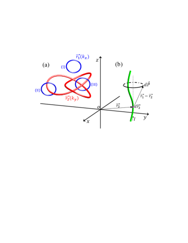
Figure 1: Schematic illustration of the aim of present work. (a) We consider a $2$D system with the Bloch Hamiltonian related to two periodic vector functions $\mathbf{r}_{1}(k_{x})$ and $\mathbf{r}_{2}(k_{y})$ in auxiliary space, which correspond to two knots. The topological index of the energy band is determined by the relations of two knots: The Chern number of the band equals to the linking number of two knots. Several representative configurations of $[\mathbf{r}_{1}(k_{x}),$ $\mathbf{r}_{2}(k_{y})]$ is presented. Here $\mathbf{r}_{2}$ is a trefoil knot, while three types of $\mathbf{r}_{1}$ are taken as simple loops, but at different positions, resulting linking numbers $\mathcal{N}=0$, $1$, and $2$, respectively. The corresponding Bloch Hamiltonians describe the systems with Chern numbers $c=0$, $1$, and $2$, respectively. (b) The main purpose of this work. For a $1$D model with a fixed function $\mathbf{r}_{2}(k_{y})$, $\mathbf{r}_{2}(k_{y})$ is referred as to the degeneracy circuit. For an arbitrary point $\mathbf{r}_{1}(k_{x})$, the polarization filed $\mathbf{P}(\mathbf{r}_{1})$ obeys the Biot-Savart law for magnetic field arising from the degeneracy loop as a current loop. Polarization field $\mathrm{d}\mathbf{P}$ at point $\mathbf{r}_{1}$ generated from an infinitesmall length of degeneracy line $\mathrm{d}\mathbf{r}_{2}$ at $\mathbf{r}_{2}$, has the identical form with the Biot-Savart Law related magnetic field generated from the current loop. Finding the polarization field $\mathbf{P}$ at arbitrary point $\mathbf{r}_{1}$ resulting from a degeneracy line can be simply obtained by the Biot-Savart law in electromagnetism.

In this work, we provide another quantum analogy of classical electromagnetism. We consider a class of Bloch Hamiltonians, which contains two periodic vector functions with respect to two independent variables, such as momentum $k_{x}$ and $k_{y}$ for a $2$D lattice system, respectively. These two periodic vector functions correspond to two knots in $3$D auxiliary space (see Fig. 1(a)). The Bloch vector is the difference of two vectors. When we only consider one of two knots, the system reduces to a $1$D lattice system. The Zak phase and polarization field at a fixed point in $3$D auxiliary space can be obtained. We show exactly that the knot as a degeneracy line has a simple relation of its corresponding polarization field, obeying the Biot-Savart law: The degeneracy line acts as a current-carrying wire, while the polarization field corresponds to the generated magnetic field. The relationship between two knots can be characterized by applying the Ampère’s circuital law on the field integral arising from one knot along another knot. For a nontrivial topological system, the integral is nonzero, due to the fact that two Bloch knots entangle with each other, forming a link with the linking number being the value of Chern number of the energy band. In Fig. 1, we schematically illustrate the main conclusion of this work.

We propose two lattice models to exemplify the application of our approach. The first one is an extended QWZ model. We show that the Bloch Hamiltonian is an example of our concerned system. Two knots of the original QWZ model simply reduce to two circles. The second one is a time-dependent quasi-$1$D model with magnetic flux. In this case, the Ampère circulation integral is equivalent to the topological invariant. In the aid of the Biot-Savart law, the pumping charge acts as a dynamic measure of the Chern number. We perform numerical simulation for several representative quasi-adiabatic processes to demonstrate this application.

The remainder of this paper is organized as follows. In Sec. II, we present a class of models, whose Bloch Hamiltonian relates to two knots. In Sec. III We propose the extended QWZ model to exemplify the application of our approach. Sec. IV gives another example, which is a time-dependent quasi-$1$D model with magnetic flux. Sec. V devotes to a dynamic measure of Chern number, the pumping charge, which can be computed numerically for several representative quasi-adiabatic processes to demonstrate our work. Finally, we present a summary and discussion in Sec. VI.

II Double-knot model

Consider a Bloch Hamiltonian $h_{\mathbf{k}}$ in the form

$$h_{\mathbf{k}} = \left(\begin{array}[]{cc}\left(z_{1}-z_{2}\right)&x_{1}-x_{2}-i\left(y_{1}-y_{2}\right)\\ x_{1}-x_{2}+i\left(y_{1}-y_{2}\right)&-\left(z_{1}-z_{2}\right)\end{array}\right)$$ (3)

$$= \left[\mathbf{r}_{1}(k_{x})\mathbf{-r}_{2}(k_{y})\right]\mathbf{\cdot\sigma},$$ (4)

which is the starting point of our study. It is consisted of two periodic vector functions $\mathbf{r}_{1}(k_{x})=\mathbf{r}_{1}(2\pi+k_{x})=x_{1}\mathbf{i}+y_{1}\mathbf{j}+z_{1}\mathbf{k}$ and $\mathbf{r}_{2}(k_{y})=\mathbf{r}_{2}(2\pi+k_{y})=x_{2}\mathbf{i}+y_{2}\mathbf{j}+z_{2}\mathbf{k}$, representing two knots (loops) in $3$D auxiliary space. Here $\mathbf{\sigma=(}\sigma_{x},\sigma_{y},\sigma_{z}\mathbf{)}$ are Pauli matrices and $h_{\mathbf{k}}$ represents a class of models, which is referred as to double-knot (double-loop) model. Matrix $h_{\mathbf{k}}$ can take the role of a core matrix of crystalline system for non-interacting Hamiltonian, or Kitaev Hamiltonian. We note that the spectrum of $h_{\mathbf{k}}$ is two-band and the gap closes when two knots have crossing points. The aim of this work is to reveal the feature of the system which is originated from the character of two knots.

To this end, we first consider the case with a fixed $k_{x}$. Then the model only contains a point $\mathbf{r}_{1}$ and a knot $\mathbf{r}_{2}\left(k_{y}\right)$. The Hamiltonian reduces to

$$h_{k_{y}}=\left[\mathbf{r}_{1}\mathbf{-r}_{2}(k_{y})\right]\mathbf{\cdot\sigma},$$ (5)

which is a $1$D system in real space. Here $r_{2}(k_{y})$ is a degeneracy line, at which the gap closes. The solution of equation $h_{k_{y}}\left|u_{\pm}^{k_{y}}\right\rangle=\varepsilon_{k_{y}}^{\pm}\left|u_{\pm}^{k_{y}}\right\rangle$ has the form

$$\left|u_{+}^{k_{y}}\right\rangle=\left(\begin{array}[]{c}\cos\frac{\theta_{k_{y}}}{2}e^{-i\varphi_{k_{y}}}\\ \sin\frac{\theta_{k_{y}}}{2}\end{array}\right),\left|u_{-}^{k_{y}}\right\rangle=i\left(\begin{array}[]{c}-\sin\frac{\theta_{k_{y}}}{2}\\ \cos\frac{\theta_{k_{y}}}{2}e^{i\varphi_{k_{y}}}\end{array}\right)$$ (6)

with $\varepsilon_{k_{y}}^{\pm}=\pm\left|\mathbf{r}_{1}\mathbf{-r}_{2}\left(k_{y}\right)\right|$, where the azimuthal and polar angles are defined as

$$\cos\theta_{k_{y}}=\frac{z_{1}-z_{2}}{\left|\mathbf{r}_{1}\mathbf{-r}_{2}\right|},\tan\varphi_{k_{y}}=\frac{y_{1}-y_{2}}{x_{1}-x_{2}}.$$ (7)

For this $1$D system, the corresponding Zak phases for upper and lower bands are defined as

$$\mathcal{Z}_{\pm}=\frac{i}{2\pi}\int_{-\pi}^{\pi}\left\langle u_{\pm}^{k_{y}}\right|\frac{\partial}{\partial k_{y}}\left|u_{\pm}^{k_{y}}\right\rangle\mathrm{d}k_{y}.$$ (8)

It is well known that the Zak phase is gauge-dependent and the present expression of $\left|u_{\pm}^{k_{y}}\right\rangle$ results in

$$\mathcal{Z}=\mathcal{Z}_{+}=-\mathcal{Z}_{-}=\frac{1}{2\pi}\oint_{\mathrm{L}}\cos^{2}\frac{\theta_{k_{y}}}{2}\mathrm{d}\varphi_{k_{y}},$$ (9)

where L denotes the integral loop about the solid angle. Accordingly, the polarization vector field is defined as

$$\mathbf{P}=-\mathbf{\nabla}\mathcal{Z},$$ (10)

where $\mathbf{\nabla}$ is the nabla operator

$$\mathbf{\nabla}=(\frac{\partial}{\partial x_{1}}\mathbf{i}+\frac{\partial}{\partial y_{1}}\mathbf{j}+\frac{\partial}{\partial z_{1}}\mathbf{k}),$$ (11)

with unitary vectors $\mathbf{i}$, $\mathbf{j}$, and $\mathbf{k}$ in $3$D auxiliary space. Straightforward derivation (see Appendix) shows that

$$\mathbf{P}=\frac{1}{4\pi}\oint_{\mathrm{L}}\frac{\mathrm{d}\mathbf{r}_{2}\times\left(\mathbf{r}_{1}-\mathbf{r}_{2}\right)}{\left|\mathbf{r}_{1}-\mathbf{r}_{2}\right|^{3}},$$ (12)

where $\mathrm{L}$ denotes the integral loop about the degeneracy loop. It is clear that if we consider a degeneracy loop as current-carrying wire with steady current strength $I=1/\mu_{0}$, flowing in the direction of increasing $k_{y}$ from $0$ to $2\pi$, the field $\mathbf{P}$ is identical to the magnetic field generated by the current loop, where $\mu_{0}$ is the vacuum permittivity of free space. Since the Eq. (12) holds for an arbitrary loop $\mathrm{L}$, one can have its differential form

$$\mathrm{d}\mathbf{P}=\frac{1}{4\pi}\frac{\mathrm{d}\mathbf{r}_{2}\times\left(\mathbf{r}_{1}-\mathbf{r}_{2}\right)}{\left|\mathbf{r}_{1}-\mathbf{r}_{2}\right|^{3}},$$ (13)

which is illustrated in Fig. 1. It indicates that the relationship between $\mathbf{P}$ and the degeneracy loop obeys the Biot-Savart law. It reveals the topological characteristics of the degeneracy lines in a clear physical picture. We will regard degeneracy loops as a band degeneracy circuit. This result helps us to determine the polarization of any loops in the auxiliary space. In addition, the Ampère circulation integral $\oint_{\ell}\mathbf{P(\mathbf{r})\cdot}\mathrm{d}\mathbf{r}$ along a loop $\ell$ has clear physical means: (i) It equals to the sum of the current through the surface spanned by the loop $\ell$; (ii) It is the pumping charge for the adiabatic passage $\ell$.

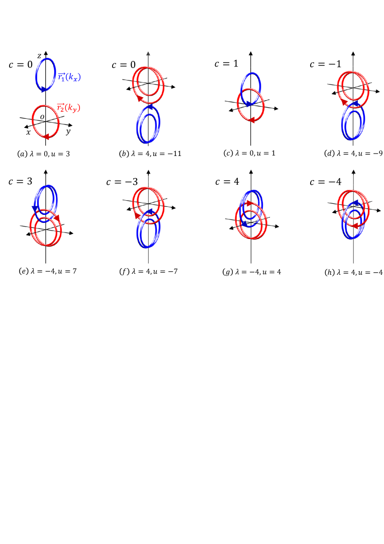
Figure 2: Schematic several representative configurations of double-knot $\left\{\mathbf{r}_{1}(k_{x}),\mathbf{r}_{2}(k_{y})\right\}$ for the extended QWZ model. The plots are obtained from parameter equations in Eq. (18) with parameters indicated in the panels. The arrows on the loops indicate the directions of the knots with various topologies. The corresponding Chern numbers are labeled, that match the linking numbers exactly.

Now we go back to $h_{\mathbf{k}}$, taking the loop $\ell$ as the knot $\mathbf{r}_{1}(k_{x})$, which has no crossing point on the knot $\mathbf{r}_{2}(k_{y})$. We find that the corresponding Ampère circulation integral is connected to the topology of two knots and the band structure of the system

$$-\oint_{\ell}\mathbf{P(\mathbf{r})\cdot}\mathrm{d}\mathbf{r=}c=\mathcal{N}\mathbf{.}$$ (14)

Here the Chern number for lower band is defined as XLQI ; GYCHO

$$c=\frac{1}{4\pi}\int_{0}^{2\pi}\int_{0}^{2\pi}\frac{\mathbf{r}^{\prime}}{\left|\mathbf{r}^{\prime}\right|^{3}}\mathbf{\cdot}\left(\frac{\partial\mathbf{r}^{\prime}}{\partial k_{x}}\times\frac{\partial\mathbf{r}^{\prime}}{\partial k_{y}}\right)\mathrm{d}k_{x}\mathrm{d}k_{y},$$ (15)

with $\mathbf{r}^{\prime}=\mathbf{r}_{1}-\mathbf{r}_{2}$, which also equals to the linking number RICCA of two knots $\mathbf{r}_{1}(k_{y})$ and $\mathbf{r}_{2}(k_{x})$

$$\mathcal{N}=\frac{1}{4\pi}\int_{0}^{2\pi}\int_{0}^{2\pi}\frac{\mathbf{r}^{\prime}}{\left|\mathbf{r}^{\prime}\right|^{3}}\mathbf{\cdot}\left(\frac{\partial\mathbf{r}_{1}}{\partial k_{x}}\times\frac{\partial\mathbf{r}_{2}}{\partial k_{y}}\right)\mathrm{d}k_{x}\mathrm{d}k_{y}.$$ (16)

These relations are evident demonstrations of the system’s topological feature and clearly reveal the physical significance of the Ampère circulation integral $\oint_{\ell}\mathbf{P(\mathbf{r})\cdot}\mathrm{d}\mathbf{r}$. Furthermore, it corresponds to the jump of Zak phase for an adiabatic passage along a knot, which can be measured by the Thouless pumping charge in a quasi $1$D system. In the following, we present two examples to illustrate our results.

III Extended QWZ model

In this section, we consider a model, which is an extension of QWZ model introduced by Qi, Wu and Zhang QWZ , to illustrate our result. The Bloch Hamiltonian is

$$h_{\mathbf{k}}=B_{x}\sigma_{x}+B_{y}\sigma_{y}+B_{z}\sigma_{z},$$ (17)

where the field components are

$$\left\{\begin{array}[]{l}B_{x}=\sin k_{x}+\lambda\sin\left(2k_{x}\right)\\ B_{y}=\sin k_{y}+\lambda\sin\left(2k_{y}\right)\\ B_{z}=u+\cos k_{x}+\cos k_{y}\\ +\lambda\left[\cos\left(2k_{x}\right)+\cos\left(2k_{y}\right)\right]\end{array}\right..$$ (18)

It reduces to original QWZ model when taking $\lambda=0$.

Now we rewrite it in the form

$$h_{\mathbf{k}}=\left[\mathbf{r}_{1}(k_{x})\mathbf{-r}_{2}(k_{y})\right]\mathbf{\cdot\sigma},$$ (19)

where two vector functions are

$$\left\{\begin{array}[]{l}\mathbf{r}_{1}=(\sin k_{x}+\lambda\sin\left(2k_{x}\right),0,u+\cos k_{x}+\lambda\cos\left(2k_{x}\right))\\ \mathbf{r}_{2}=-(0,\sin k_{y}+\lambda\sin\left(2k_{y}\right),\cos k_{y}+\lambda\cos\left(2k_{y}\right))\end{array}\right..$$ (20)

It is clear that $\mathbf{r}_{1}(k_{x})$ and $\mathbf{r}_{2}(k_{y})$ represent two limacons within $xz$ and $yz$ plane, respectively. When taking $\left|\lambda\right|<0.5$, the crossing point of the limacon disappears. Particularly, when taking $\lambda=0$, limacons reduce to circles. The radiuses of two circles are both $1$, but the centers are $(0,0,u)$ and $(0,0,0)$, respectively. Chern numbers can be easily obtained from the linking numbers of these two circles: $c=0$, for $\left|u\right|>2$, and $c=\pm 1$, for $0<\pm u<2$. When taking $\left|\lambda\right|>0.5$, the crossing point of the limacon appears. Since limacons with crossing point cannot be classified as knots, we add perturbation terms $\kappa\sin 2k_{x}$ to $r_{1y}$ and $\kappa\sin 2k_{y}$ to $r_{2x}$ to untie the crossing point ($\left|\kappa\right|\ll 1$), then limacons become knots again. The possible linking numbers of such two knots are still equal to the Chern numbers $c=0$, $\pm 1$, $\pm 3$, and $\pm 4$. The absence of $c=\pm 2$ is due to the fact that we take the identical $\lambda$ in the expressions of $\mathbf{r}_{1}(k_{x})$ and $\mathbf{r}_{2}(k_{y})$. In Fig. 2, we plot some representative configurations to demonstrate this point. Comparing to the direct calculation of Chern number from the Berry connection, the example shows that the Chern number can be easily obtained by the geometrical configurations hidden in the Bloch Hamiltonian.

IV Ladder system

As a simple application of our result, we consider a quasi $1$D system with periodically time-dependent parameters. The Bloch Hamiltonian has the form

$$h_{k}(t)=\left[\mathbf{r}(t)\mathbf{-r}_{c}(k)\right]\mathbf{\cdot\sigma},$$ (21)

where $\mathbf{r}(t)=\mathbf{r}(t+T)$ represents a loop $\ell$ without crossing point on the degeneracy loop $\mathbf{r}_{c}(k)$. The result obtained above still apply to the case of replacing $(k_{x},k_{y})$ with $(t,k)$, and replacing $\left|u_{\pm}^{\mathbf{k}}\right\rangle$ with $|u_{\pm}^{k}(t)\rangle$ accordingly. In this section we will demonstrate our result and its physical implications through an alternative tight-binding model, which is two coupled SSH chains, or a ladder system with staggered magnetic flux, on-site potential and long range hopping terms. These ingredients allow the system to support multiple types of degeneracy loops with different geometric topologies.

We consider a ladder system which is illustrated in Fig. 3, represented by the Hamiltonian

$$H_{\text{L}}=\sum_{j=1}^{N}\{r_{\bot}e^{i\phi}c_{2j}^{{\dagger}}c_{2j-1}+\alpha c_{2j-1}^{{\dagger}}c_{2\left(j+1\right)}+\beta c_{2\left(j+1\right)-1}^{{\dagger}}c_{2j}$$

$$+\mu c_{2\left(j+2\right)-1}^{{\dagger}}c_{2j}+\nu c_{2j-1}^{{\dagger}}c_{2\left(j+2\right)}+i\kappa[c_{2\left(j+3\right)-1}^{{\dagger}}c_{2j-1}$$

$$-c_{2\left(j+3\right)}^{{\dagger}}c_{2j}]+\text{{H.c.}}\}+z\sum_{j=1}^{2N}\left(-1\right)^{j+1}c_{j}^{{\dagger}}c_{j},$$ (22)

on a $2N$ lattice. Here $c_{j}^{{\dagger}}$ is the creation operator of a fermion at the $j$th site with the periodic boundary condition $c_{2N+1}=c_{1}$. The inter-sublattice hopping amplitudes are $\left(\alpha,\beta,\mu,\nu\right)$ and the intra-sublattice hopping amplitude is $\kappa$. Besides, two time-dependent parameters, $2\phi(t)$ is the staggered magnetic flux threading each plaquette and $z(t)$ is the strength of staggered potentials. The ladder system is essentially two coupled SSH chains. As a building block of the system, the SSH model SSH has served as a paradigmatic example of the $1$D system supporting topological character Zak . It has an extremely simple form but well manifests the typical feature of topological insulating phase, and the transition between non-trivial and trivial topological phases, associated with the number of zero energy and edge states as the topological invariant Asboth . It has been demonstrated that all the parameters of this model can be easily accessed within the existing technology of cold-atomic experiments Clay ; Ueda ; Jo . We schematically illustrate this model in Fig. 3. We introduce the fermionic operators in $k$ space

$$\left\{\begin{array}[]{l}a_{k}=\frac{1}{\sqrt{N}}\sum_{j=1}^{N}e^{-ikj}c_{2j-1}\\ b_{k}=\frac{1}{\sqrt{N}}\sum_{j=1}^{N}e^{-ikj}c_{2j}\end{array}\right.,$$ (23)

and the wave vector $k=\pi(2n-N)/N$, $(n=0,1,...,N-1)$. Then we have

$$H_{\text{L}}=\sum_{k}(a_{k}^{\dagger},b_{k}^{\dagger})h_{k}\left(\begin{array}[]{c}a_{k}\\ b_{k}\end{array}\right),$$ (24)

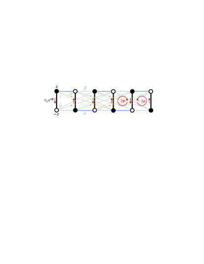
Figure 3: Schematics of the two coupled SSH chains with staggered flux and potential. The system consists of two sublattices A and B with on-site potentials $z$ and $-z$, indicated by filled and empty circles, respectively. Hopping amplitudes along each chain are staggered by $\alpha$ (blue solid line) and $\beta$ (blue dotted line). The interchain hopping amplitude is $r_{\perp}$ (thick black line) associated with a phase factor and interchain diagonal hopping amplitude $\mu$ (gray solid line), $\nu$ (gray dotted line) and $i\kappa$ (light green solid line). The red arrows indicate the hopping directions for complex amplitudes, which are induced by the staggered flux threading each plaquettes (arrow circles).

where the core matrix has the form

$$h_{k}=\left(\begin{array}[]{cc}z+2\kappa\sin\left(3k\right)&R(\phi,k)\\ R^{\ast}(\phi,k)&-z-2\kappa\sin\left(3k\right)\end{array}\right),$$ (25)

and the off-diagonal matrix element is

$$R(\phi,k)=r_{\bot}e^{-i\phi}+\alpha e^{ik}+\beta e^{-ik}+\mu e^{-2ik}+\nu e^{2ik}.$$ (26)

Taking

$$x+iy=r_{\bot}e^{i\phi},$$ (27)

the parameter equations for degeneracy loop is

$$\left\{\begin{array}[]{l}x_{c}=-\left(\alpha+\beta\right)\cos k-\left(\mu+\nu\right)\cos\left(2k\right)\\ y_{c}=-\left(\beta-\alpha\right)\sin k-\left(\mu-\nu\right)\sin\left(2k\right)\\ z_{c}=-2\kappa\sin\left(3k\right)\end{array}\right.,$$ (28)

which is plotted in Fig. 4 for the case with parameters $\alpha=\mu=0.5$, $\beta=1$, $\nu=1.5$, and $\kappa=0.1$. One can see that the degeneracy curve is a trefoil knot. Intuitively, it should result in topological features with indices $2$, $1$, and $0$. We will demonstrate this point in the next section.

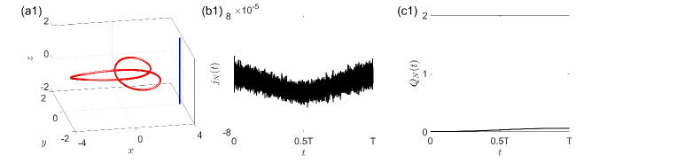
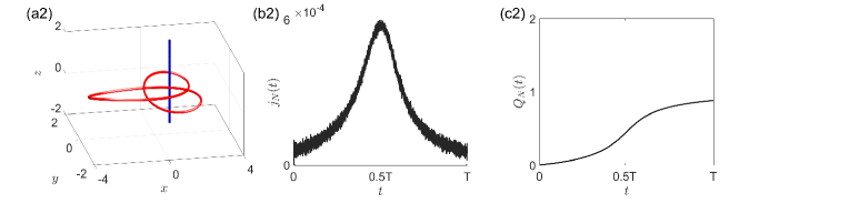
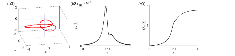
Figure 4: (a1-a3) Schematics of three adiabatic passages in $3$D auxiliary space for pumping charge. The degeneracy curve (red) is a trefoil knot with parameters $\alpha=\mu=0.5$, $\beta=1$, $\nu=1.5$, and $\kappa=0.1$ of the system in Eq. (22) (Fig. 3). The adiabatic passages are straight lines (blue) at positions $(x,y):$ (a1) $(3.80,0)$, (a2) $(1.15,0.84)$, and (a3) $(0.40,0.01)$, respectively. (b1-b3) and (c1-c3) are plots of current and the corresponding total charge transfer for quasi-adiabatic process. The results are obtained by numerically exact diagonalization method for the system in Eq. (22) with $N=100$. The speed of time evolution is $\omega=1\times 10^{-3}$. It indicates that the topological invariant can be obtained by dynamical process.

V Pumping charge

For a $2$D system with Bloch Hamiltonian in the form of Eq. (4), the physical and geometric meanings of Chern number is well established. For a quasi $1$D system with Bloch Hamiltonian in the form of Eq. (4) by replacing $(k_{x},k_{y})$ with $(t,k)$, the Chern number is connected to an adiabatic passage driven by the parameters from $t$ to $t+T$, or a periodic loop $\mathbf{r=r}(t)$ in auxiliary space. In a $1$D model, it has been shown that the adiabatic particle transport over a time period takes the form of the Chern number and it is quantized DXIAO . The pumped charge counts the net number of degeneracy point enclosed by the loop. This can be extended to the loop $\mathbf{r=r}(t)$ in the present model.

Actually, one can rewrite Eq. (14) in the form

$$c=\mathcal{N}=-\oint_{\ell}\mathbf{P(\mathbf{r})\cdot}\frac{\partial\mathbf{\mathbf{r}}}{\partial t}\mathrm{d}t\mathbf{.}$$ (29)

where $\mathbf{\mathbf{r}}$ (or $r_{\bot},\phi,$ and $z$) is periodic function of time $t$. Furthermore, we can find out the physical meaning of the Chern number by the relation

$$c=\int_{0}^{T}\mathcal{J}(t)\mathrm{d}t,$$ (30)

where

$$\mathcal{J}=\frac{i}{2\pi}\int_{0}^{2\pi}[(\partial_{t}\langle u_{-}^{k}|)\partial_{k}|u_{-}^{k}\rangle-(\partial_{k}\langle u_{-}^{k}|)\partial_{t}|u_{-}^{k}\rangle]\mathrm{d}k$$ (31)

is the adiabatic current. Then $c$ is pumped charge of all channel $k$ driven by the time-dependent Hamiltonian varying in a period, which can be measured through a quasi adiabatic process.

Inspired by these analysis, we expect that the Chern number can be unveiled by the pumping charge of all the energy levels. This can be done in single-particle sub-space. The accumulated charge passing the unit cell $l$ during the period $T$ is

$$Q_{l}=\sum_{k}\int_{0}^{T}j_{l}\mathrm{d}t,$$ (32)

where current across two neighboring unit cells is

$$j_{l}=\frac{1}{i}\left\langle u_{-}^{k}\left(t\right)\right|[\alpha a_{j}^{{\dagger}}b_{j+1}+\beta b_{j}^{{\dagger}}a_{j+1}+\mu b_{j}^{{\dagger}}a_{j+2}+$$

$$\nu a_{j}^{{\dagger}}b_{j+2}-i\kappa a_{j}^{{\dagger}}a_{j+3}+i\kappa b_{j}^{{\dagger}}b_{j+3}-\text{{H.c.}}]\left|u_{-}^{k}\left(t\right)\right\rangle.$$ (33)

As we mentioned above, there are three types of adiabatic loop $\mathbf{r=r}(t)$ in auxiliary space, with pumping charges $Q_{l}=0$, $1$, and $2$, respectively. In general, three periodic functions $r_{\bot}(t)$, $\phi(t)$, and $z(t)$ should be taken to measure the pumping charge. However, a quasi adiabatic loop is tough to be realized in practice. Thanks to the Biot-Savart law for the field $\mathbf{P}(r)$, we can take the adiabatic passage along a straight line with fixed $r_{\bot}$ and $\phi$, since the field $\mathbf{P}$ far from the trefoil knot $\mathbf{r}_{c}(k)$ has no contribution to the Ampère circulation integral, or the pumping charge.

We consider the case by taking $z=\omega t$ with $\omega\ll 1$. According to the analysis above, if $t$ varies from $-\infty$ to $\infty$, $Q_{l}$ should be $0$, $1$, and $2$, respectively. To examine how the scheme works in practice, we simulate the quasi-adiabatic process by computing the time evolution numerically for finite system. In principle, for a given initial eigenstate $\left|u_{-}^{k}\left(0\right)\right\rangle$, the time evolved state under a Hamiltonian $H_{\text{L}}\left(t\right)$ is

$$\left|\Phi\left(t\right)\right\rangle=\mathcal{T}\{\exp(-i\int_{0}^{t}H_{\text{L}}\left(t\right)\mathrm{d}t)\left|u_{-}^{k}\left(0\right)\right\rangle\},$$ (34)

where $\mathcal{T}$ is the time-ordered operator. In low speed limit $\omega\rightarrow 0$, we have

$$f\left(t\right)=\left|\langle u_{-}^{k}\left(t\right)\left|\Phi\left(t\right)\right\rangle\right|\rightarrow 1,$$ (35)

where $\left|u_{-}^{k}\left(t\right)\right\rangle$ is the corresponding instantaneous eigenstate of $H_{\text{L}}\left(t\right)$. The computation is performed by using a uniform mesh in the time discretization for the time-dependent Hamiltonian $H_{\text{L}}$. In order to demonstrate a quasi-adiabatic process, we keep $f\left(t\right)>0.9$ during the whole process by taking sufficient small $\omega$. Fig. 4 plots the simulations of particle current and the corresponding total probability, which shows that the obtained dynamical quantities are in close agreement with the expected Chern number.

VI Summary and discussion

We have analyzed a family of $2$D tight-binding model with various Chern numbers, which are directly connected to the topology of two knots. When reduced to $1$D single-knot degeneracy model, a polarization vector field can be established for a gapped band. We have exactly shown an interesting analogy between the topological feature of the band and classical electromagnetism: polarization vector field acts as the static magnetic field generated by the degeneracy knot as a current circuit. It indicates that there is a quantum analogy of Biot-Savart law in quantum matter. Before ending this paper, we would like to point out that our findings also reveal the topological feature hidden in the case with zero Chern number. In Fig. 2(a) and (b), we find out that though the linking numbers of these two sets of loops are zero, the configurations are different. It should imply certain topological feature in a single direction, which will be investigated in future work. This finding extends the understanding of topological feature in matter and provides methodology and tool for dealing with the calculation and detection of Chern numbers.

VII Appendix: Proof of the Biot-Savart law

In this appendix, we provide the proof of Eq. (12) in the main text. To this end, we first revisit the Biot-Savart law for a current carrying loop, and then compare it with the polarization field in the present work.

VII.1 The magnetic field

Consider a current carrying loop $\mathrm{L}$ with current strength $I=1/\mu_{0}$, which is described by a periodic function $\mathbf{r}_{2}\left(k_{y}\right)=x_{2}\mathbf{i+}y_{2}\mathbf{j+}z_{2}\mathbf{k}$ in a $3$D space. Here $\mu_{0}$ is the vacuum permittivity of free space and the current flows in the direction of increasing $k_{y}$ from $0$ to $2\pi$. According to the Biot-Savart law, the magnetic field $\mathbf{B}$ at position $\mathbf{r}_{1}=x_{1}\mathbf{i+}y_{1}\mathbf{j+}z_{1}\mathbf{k}$ generated by the loop $\mathrm{L}$ is

$$\mathbf{B}=\frac{1}{4\pi}\oint_{\mathrm{L}}\frac{\mathbf{r}_{2}-\mathbf{r}_{1}}{\left|\mathbf{r}_{1}-\mathbf{r}_{2}\right|^{3}}\times\mathrm{d}\mathbf{r}_{2}.$$ (36)

For the sake of simplicity we only give the proof for $\mathbf{B}$ and $\mathbf{P}$ in the $x$ component as an example. The explicit form of the component is

$$B_{x}=\frac{1}{4\pi}\oint_{\mathrm{L}}\frac{\left(y_{2}-y_{1}\right)\mathrm{d}z_{2}\mathbf{-}\left(z_{2}-z_{1}\right)\mathrm{d}y_{2}}{\left|\mathbf{r}_{1}-\mathbf{r}_{2}\right|^{3}}.$$ (37)

According to the Stokes’ theorem, the line integral of $B_{x}$ can be expressed as a double integral

$$B_{x} = \frac{1}{4\pi}\iint\nolimits_{\mathrm{S}}[\frac{3\left(x_{2}-x_{1}\right)^{2}-\left|\mathbf{r}_{1}-\mathbf{r}_{2}\right|^{2}}{\left|\mathbf{r}_{1}-\mathbf{r}_{2}\right|^{5}}\mathrm{d}y_{2}\mathrm{d}z_{2}$$ (38)

$$-\frac{3\left(x_{2}-x_{1}\right)\left(y_{1}-y_{2}\right)}{\left|\mathbf{r}_{1}-\mathbf{r}_{2}\right|^{5}}\mathrm{d}z_{2}\mathrm{d}x_{2}$$

$$-\frac{3\left(x_{2}-x_{1}\right)\left(z_{1}-z_{2}\right)}{\left|\mathbf{r}_{1}-\mathbf{r}_{2}\right|^{5}}\mathrm{d}x_{2}\mathrm{d}y_{2}],$$

where $S$ represents a smooth surface spanned by the loop $L$.

VII.2 The polarization vector field

Now we turn to the quantum analogy of Biot-Savart law. For a fixed $k_{x}$, $h_{\mathbf{k}}$ reduces to a $1$D system $h_{k_{y}}$, and the corresponding Zak phases for upper and lower bands are defined as

$$\mathcal{Z}_{\pm}=\frac{i}{2\pi}\int_{-\pi}^{\pi}\left\langle u_{\pm}^{k_{y}}\right|\frac{\partial}{\partial k_{y}}\left|u_{\pm}^{k_{y}}\right\rangle\mathrm{d}k_{y},$$ (39)

which is gauge-dependent. For the present expression of $\left|u_{\pm}^{k_{y}}\right\rangle$, we have

$$\mathcal{Z}=\mathcal{Z}_{+}=-\mathcal{Z}_{-}=\frac{1}{2\pi}\oint_{\mathrm{L}}\cos^{2}\frac{\theta}{2}\mathrm{d}\varphi,$$ (40)

where $\mathrm{L}$ denotes loop $\mathbf{r}_{2}(k_{y})$ and

$$\cos\theta=\frac{z_{1}-z_{2}}{\left|\mathbf{r}_{1}-\mathbf{r}_{2}\right|},\tan\varphi=\frac{y_{1}-y_{2}}{x_{1}-x_{2}}.$$ (41)

The polarization vector field is defined as

$$\mathbf{P}=-\mathbf{\nabla}\mathcal{Z},$$ (42)

where $\mathbf{\nabla}$ is the nabla operator

$$\mathbf{\nabla}=(\frac{\partial}{\partial x_{1}}\mathbf{i}+\frac{\partial}{\partial y_{1}}\mathbf{j}+\frac{\partial}{\partial z_{1}}\mathbf{k}),$$ (43)

with unitary vectors $\mathbf{i}$, $\mathbf{j}$, and $\mathbf{k}$ in $3$D auxiliary space. We note the fact that

$$\mathbf{k\cdot[}\oint_{\mathrm{L}}\frac{\mathbf{r}_{2\bot}-\mathbf{r}_{1\bot}}{\left|\mathbf{r}_{2\bot}-\mathbf{r}_{1\bot}\right|^{2}}\times\mathrm{d}\left(\mathbf{r}_{2\bot}-\mathbf{r}_{1\bot}\right)]=\oint_{\mathrm{L}}\mathrm{d}\varphi=2\pi w,$$ (44)

where $w$ is winding number of the integral loop $\mathbf{r}_{2\bot}(k_{y})=x_{2}\mathbf{i}+y_{2}\mathbf{j}$ around the point $\mathbf{r}_{1\bot}=x_{1}\mathbf{i}+y_{1}\mathbf{j}$. Then the Zak phase can be rewritten as

$$\mathcal{Z}=\frac{\mathbf{k}}{4\pi}\mathbf{\cdot}\oint_{\mathrm{L}}\left[1+\frac{z_{1}-z_{2}}{\left|\mathbf{r}_{1}-\mathbf{r}_{2}\right|}\right]\frac{\mathbf{r}_{2\bot}-\mathbf{r}_{1\bot}}{\left|\mathbf{r}_{2\bot}-\mathbf{r}_{1\bot}\right|^{2}}\times\mathrm{d}\left(\mathbf{r}_{2\bot}-\mathbf{r}_{1\bot}\right).$$ (45)

The projection of the polarization vector field $\mathbf{P}$ in the $x$ direction is represented as

$$P_{x}=-\frac{\partial}{\partial x_{1}}\mathcal{Z}=\frac{1}{4\pi}\oint_{\mathrm{L}}\left(G\mathrm{d}x_{2}+Q\mathrm{d}y_{2}+R\mathrm{d}z_{2}\right),$$ (46)

where

$$G = -\frac{\left(z_{1}-z_{2}\right)\left(x_{2}-x_{1}\right)\left(y_{2}-y_{1}\right)}{\left|\mathbf{r}_{1}-\mathbf{r}_{2}\right|^{3}\left|\mathbf{r}_{2\bot}-\mathbf{r}_{1\bot}\right|^{2}}$$

$$-\left(1+\frac{z_{1}-z_{2}}{\left|\mathbf{r}_{1}-\mathbf{r}_{2}\right|}\right)\frac{2\left(x_{2}-x_{1}\right)(y_{2}-y_{1})}{\left|\mathbf{r}_{2\bot}-\mathbf{r}_{1\bot}\right|^{4}},$$

and

$$Q = \left(1+\frac{z_{1}-z_{2}}{\left|\mathbf{r}_{1}-\mathbf{r}_{2}\right|}\right)\frac{\left[\left(x_{2}-x_{1}\right)^{2}-\left(y_{2}-y_{1}\right)^{2}\right]}{\left|\mathbf{r}_{2\bot}-\mathbf{r}_{1\bot}\right|^{4}}$$ (48)

$$+\frac{\left(z_{1}-z_{2}\right)\left(x_{2}-x_{1}\right)^{2}}{\left|\mathbf{r}_{1}-\mathbf{r}_{2}\right|^{3}\left|\mathbf{r}_{2\bot}-\mathbf{r}_{1\bot}\right|^{2}}.$$

By the Stokes’ theorem, the line integral of $P_{x}$ can be expressed as a double integral

$$P_{x} = \frac{1}{4\pi}\iint\nolimits_{\mathrm{S}}[\frac{3\left(x_{2}-x_{1}\right)^{2}-\left|\mathbf{r}_{1}-\mathbf{r}_{2}\right|^{2}}{\left|\mathbf{r}_{1}-\mathbf{r}_{2}\right|^{5}}\mathrm{d}y_{2}\mathrm{d}z_{2}$$ (49)

$$-\frac{3\left(x_{2}-x_{1}\right)\left(y_{1}-y_{2}\right)\allowbreak}{\left|r_{2}-r_{1}\right|^{5}}\mathrm{d}z_{2}\mathrm{d}x_{2}$$

$$-\frac{3\left(x_{1}-x_{2}\right)\left(z_{2}-z_{1}\right)}{\left|\mathbf{r}_{1}-\mathbf{r}_{2}\right|^{5}}\mathrm{d}x_{2}\mathrm{d}y_{2}],$$

which results in

$$P_{x}=B_{x}.$$ (50)

Similarly, the projection of polarization vector field $\mathbf{P}$ and magnetic field $\mathbf{B}$ in the $y$ and $z$ direction can be calculated in the same way. Eventually, we can come to a conclusion

$$\mathbf{P}=\mathbf{B}=\frac{1}{4\pi}\oint_{\mathrm{L}}\frac{\mathbf{r}_{2}-\mathbf{r}_{1}}{\left|\mathbf{r}_{1}-\mathbf{r}_{2}\right|^{3}}\times\mathrm{d}\mathbf{r}_{2}.$$ (51)

- (1) X. Wan, A. M. Turner, A. Vishwanath, and S. Y. Savrasov, Topological semimetal and Fermi-arc surface states in the electronic structure of pyrochlore iridates, Phys. Rev. B 83, 205101 (2011).
- (2) L. Lu, L. Fu, J. D. Joannopoulos, and M. Soljačić, Weyl points and line nodes in gyroid photonic crystals, Nature Photon. 7, 294–299 (2013).
- (3) S.-M. Huang, S.-Y. Xu, I. Belopolski, C.-C. Lee, G. Chang, B. Wang, N. Alidoust, G. Bian, M. Neupane, A. Bansil et al., A Weyl Fermion semimetal with surface Fermi arcs in the transition metal monopnictide TaAs class, Nature Commun. 6, 7373 (2015).
- (4) H. Weng, C. Fang, Z. Fang, B. A. Bernevig, and X. Dai, Weyl Semimetal Phase in Noncentrosymmetric Transition-Metal Monophosphides, Phys. Rev. X 5, 011029 (2015).
- (5) S.-Y. Xu, I. Belopolski, N. Alidoust, M. Neupane, G. Bian, C. Zhang, R. Sankar, G. Chang, Z. Yuan, C.-C. Lee, M. Z. Hasan et al., Discovery of a Weyl fermion semimetal and topological Fermi arcs, Science 349, 613–617 (2015).
- (6) B. Q. Lv, H. M. Weng, B. B. Fu, X. P. Wang, H. Miao, J. Ma, P. Richard, X. C. Huang, L. X. Zhao, G. F. Chen, Z. Fang, X. Dai, T. Qian, and H. Ding, Experimental Discovery of Weyl Semimetal TaAs, Phys. Rev. X 5, 031013 (2015).
- (7) L. Lu, Z. Wang, D. Ye, L. Ran, L. Fu, J. D. Joannopoulos, and M. Soljačić, Experimental observation of Weyl points, Science 349, 622–624 (2015).
- (8) V. Mourik, K. Zuo, S. M. Frolov, S. R. Plissard, E. P. A. M. Bakkers, L. P. Kouwenhoven, Signatures of Majorana Fermions in Hybrid Superconductor-Semiconductor Nanowire Devices, Science 336, 1003–1007 (2012).
- (9) S. Nadj-Perge, I. K. Drozdov, J. Li, H. Chen, S. Jeon, J. Seo, A. H. MacDonald, B. A. Bernevig, and A. Yazdani, Observation of Majorana fermions in ferromagnetic atomic chains on a superconductor, Science 346, 602–607 (2014).
- (10) P.A.M. Dirac, Quantized singularities in the electromagnetic field, Proc. Royal Soc. London , A133 60 (1931).
- (11) D. Xiao, M.-C. Chang, and Q. Niu, Berry phase effects on electronic properties, Rev. Mod. Phys. 82, 1959 (2010).
- (12) A. A. Burkov, M. D. Hook, and L. Balents, Topological nodal semimetals, Phys. Rev. B 84, 235126 (2011).
- (13) T. Bzdusek, Q. Wu, A. Rüegg, M. Sigrist, and A. A. Soluyanov, Nodal-chain metals, Nature (London) 538, 75 (2016).
- (14) Z. Yan, R. Bi, H. Shen, L. Lu, S.-C. Zhang, and Z. Wang, Nodal-link semimetals, Phys. Rev. B 96, 041103 (2017).
- (15) R. Bi, Z. Yan, L. Lu, and Z.Wang, Nodal-knot semimetals, Phys. Rev. B 96, 201305 (2017).
- (16) X.-Q. Sun, B. Lian, and S.-C. Zhang, Double helix nodal line superconductor, Phys. Rev. Lett. 119, 147001 (2017).
- (17) S. Nie, H. Weng, and F. B. Prinz, Topological nodal-line semimetals in ferromagnetic rare-earth-metal monohalides, Phys. Rev. B 99, 035125 (2019).
- (18) J. Ahn, D. Kim, Y. Kim, and B.-J. Yang, Band Topology and Linking Structure of Nodal Line Semimetals with Monopole Charges, Phys. Rev. Lett. 121, 106403 (2018).
- (19) C. Fang, H. Weng, X. Dai, and Z. Fang, Topological nodal line semimetals, Chin. Phys. B 25, 117106 (2016).
- (20) T. Kawakami and X. Hu, Symmetry-guaranteed and accidental nodal-line semimetals in fcc lattice, Phys. Rev. B 96, 235307 (2017).
- (21) J. Y. Lin, N. C. Hu, Y. Jian Chen, C. H. Lee, and X. Zhang, Line nodes, Dirac points, and Lifshitz transition in two-dimensional nonsymmorphic photonic crystals, Phys. Rev. B 96, 075438 (2017).
- (22) C. Fang, Y. Chen, H.-Y. Kee, and L. Fu, Topological nodal line semimetals with and without spin-orbital coupling, Phys. Rev. B 92, 081201 (2015).
- (23) P. Y. Chang and C. H. Yee, Weyl-link semimetals, Phys. Rev. B 96, 081114 (2017).
- (24) W. Chen, H. Z. Lu, and J. M. Hou, Topological semimetals with a double-helix nodal link, Phys. Rev. B 96, 041102 (2017).
- (25) M. Ezawa, Topological semimetals carrying arbitrary Hopf numbers, Phys. Rev. B 96, 041202(R) (2017).
- (26) Y. Zhou, F. Xiong, X. Wan, and J. An, Hopf-link topological nodal-loop semimetals, Phys. Rev. B 97, 155140 (2018).
- (27) Z. Yang, C,-K, Chiu, C. Fang, and J. Hu, Jones Polynomial and Knot Transitions in Hermitian and non-Hermitian Topological Semimetals, Phys. Rev. Lett. 124, 186402 (2020).
- (28) M. Xiao and S. Fan, Topologically charged nodal surface, arXiv:1709.02363.
- (29) Q. Xu, R. Yu, Z. Fang, X. Dai, and H. Weng, Topological nodal line semimetals in the CaP3 family of materials, Phys. Rev. B 95, 045136 (2017).
- (30) R. Yu, Q. Wu, Z. Fang, and H. Weng, From Nodal Chain Semimetal to Weyl Semimetal in HfC, Phys. Rev. Lett. 119, 036401 (2017).
- (31) Q. Yan, R. Liu, Z. Yan, B. Liu, H. Chen, Z. Wang, and L. Lu, Experimental discovery of nodal chains, Nat. Phys. 14, 461-464 (2018).
- (32) G. Chang, S.-Y. Xu, X. Zhou, S.-M. Huang, B. Singh, B. Wang, I. Belopolski, J. Yin, S. Zhang, A. Bansil, H. Lin, and M. Z. Hasan, Topological Hopf and Chain Link Semimetal States and Their Application to Co2MnGa, Phys. Rev. Lett. 119, 156401 (2017).
- (33) X. Feng, C. Yue, Z. Song, Q. Wu, and B. Wen, Topological Dirac nodal-net fermions in AlB2-type TiB2 and ZrB2, Phy. Rev. Materials 2, 014202 (2018).
- (34) R. Wang, C. Li, X. Z. Zhang, and Z. Song, Dynamical bulk-edge correspondence for degeneracy lines in parameter space, Phys. Rev. B 98, 014303 (2018).
- (35) X.-L. Qi and S.-C. Zhang, Topological insulators and superconductors, Rev. Mod.Phys. 83, 1057 (2011).
- (36) G. Y. Cho and J. E. Moore, Quantum phase transition and fractional excitations in a topological insulator thin film with Zeeman and excitonic masses, Phys. Rev. B 84, 165101 (2011).
- (37) R. L. Ricca and B. Nipoti, Gauss’ linking number revisited, J. Knot Theory Ramif. 20, 1325 (2011).
- (38) X.-L. Qi, Y.-S. Wu, and S.-C. Zhang, Topological quantization of the spin hall effect in two-dimensional paramagnetic semiconductors, Phys. Rev. B 74, 085308 (2006).
- (39) W. P. Su, J. R. Schrieffer, and A. J. Heeger, Solitons in Polyacetylene, Phys. Rev. Lett. 42, 1698 (1979).
- (40) J. Zak, Berry’s phase for energy bands in solids, Phys. Rev. Lett. 62, 2747 (1989).
- (41) J. K. Asbóth, L. Oroszlány, and A. Pályi, A Short Course on Topological Insulators: Band Structure and Edge States in One and Two Dimensions, Lecture Notes in Physics (Springer International Publishing, Switzerland, 2016).
- (42) R. T. Clay and S. Mazumdar, Cooperative Density Wave and Giant Spin Gap in the Quarter-Filled Zigzag Electron Ladder, Phys. Rev. Lett. 94, 207206 (2005).
- (43) Y. Shimizu, S. Aoyama, T. Jinno, M. Itoh, and Y. Ueda, Site-Selective Mott Transition in a Quasi-One-Dimensional Vanadate V6O13, Phys. Rev. Lett. 114, 166403 (2015).
- (44) T. Zhang and G. B. Jo, One-dimensional sawtooth and zigzag lattices for ultracold atoms, Sci. Rep. 5, 16044 (2015).