Semiglobal exponential input-to-state stability of sampled-data systems based on approximate discrete-time models

Abstract

Exact discrete-time models of nonlinear systems are difficult or impossible to obtain, and hence approximate models may be employed for control design. Most existing results provide conditions under which the stability of the approximate model in closed-loop carries over to the stability of the (unknown) exact model but only in a practical sense, i.e. the trajectories of the closed-loop system are ensured to converge to a bounded region whose size can be made as small as desired by limiting the maximum sampling period. In addition, some very stringent conditions exist for the exact model to exhibit exactly the same type of asymptotic stability as the approximate model. In this context, our main contribution consists in providing less stringent conditions by considering semiglobal exponential input-to-state stability (SE-ISS), where the inputs can successfully represent state-measurement and actuation errors. These conditions are based on establishing SE-ISS for an adequate approximate model and are applicable both under uniform and nonuniform sampling. As a second contribution, we show that explicit Runge-Kutta models satisfy our conditions and can hence be employed. An example of control design for stabilization based on approximate discrete-time models is also given.

1 Introduction

Modern digital control applications involve measuring the available signals of the continuous-time plant via a sampling mechanism and then applying the computed control action via zero-order hold (ZOH). One of the existing approaches for control design consists in designing a discrete-time control law based on a discrete/time model of the plant. For nonlinear systems the exact discrete/time model, i.e. the model that exactly matches the state of the continuous-time system at sampling instants, may be difficult (or impossible) to derive due to the complexity (or non-existence) of the closed form solutions of the equations that describe the plant dynamics. Thus, the usual approach is to design the control law based on a (sufficiently good) approximate discrete-time model.

In this context, several results have been derived in order to establish different kinds of stability properties of the exact model or generate adequate approximate models [Nešić et al., 1999, Nešić and Laila, 2002, Nešić and Teel, 2004, Karafyllis and Kravaris, 2009, Nešić et al., 2009, Monaco and Normand-Cyrot, 2007, Yuz and Goodwin, 2014, van de Wouw et al., 2012, Zeng et al., 2017]. These results usually provide conditions that ensure certain kind of stability property for the approximate closed-loop model and, if the exact and approximate models satisfy some consistency property, also ensure that the stability property or a practical version of it is also fulfilled by the exact model for sufficiently small sampling periods. These stability properties contemplate a wide range of situations with respect to the uniformity of the sampling (periodic or aperiodic), the nature of the convergence to an equilibrium point (asymptotic or practical), the consideration of disturbances (input-to-state stability properties) and the nature of the maximum allowable sampling period (semiglobal or global). Several works address problems such as the presence of time delays [Di Ferdinando and Pepe, 2017, 2019, Di Ferdinando et al., 2019], observer design [Arcak and Nešić, 2004, Postoyan and Nešić, 2012, Beikzadeh and Marquez, 2016], and control schemes involving dual-rate [Liu et al., 2008, Üstüntürk, 2012] or multirate [Beikzadeh and Marquez, 2015, Polushin and Marquez, 2004] sampling. Other approaches for sampled-data stabilization only contemplate emulated controllers [Nešić et al., 2009] or require Lyapunov-like assumptions on the continuous/time plant [Nešić et al., 2009, Abdelrahim et al., 2017]. A recent publication [Lin, 2020] shows that global asymptotic and local exponential stabilizability of the continuous-time plant by state feedback imply semiglobal asymptotic stabilizability by digital state feedback; these results hold under uniform sampling. In Vallarella and Haimovich [2018], we derived necessary and sufficient conditions for (i) semiglobal asymptotic stability, robustly with respect to bounded disturbances, and (ii) semiglobal ISS, where the (disturbance) input may successfully represent state-measurement or actuation errors, both for discrete-time models of nonuniformly sampled (i.e. periodic or aperiodic) nonlinear systems. These properties are semiglobal only in the sampling period, meaning that a bound on the state exists such that for every bound on the initial condition (and input), a maximum sampling period exists for which the state bound holds. In Vallarella and Haimovich [2019], we have shown that if a consistency property (MSEC) holds between the approximate and exact closed-loop models then the smaller the maximum admissible sampling period is, the lower the error between their solutions over a fixed time period becomes. Moreover, if the control law renders the approximate model semiglobal practical ISS under nonuniform sampling (SP-ISS-VSR), then the same controller ensures SP-ISS-VSR of the exact closed/loop model. In all of these existing results, stability of the exact model is either semiglobal and practical or global and asymptotic. The conditions for ensuring global stability are stringent. To the best of the authors’ knowledge, results based on approximate discrete-time models, ensuring semiglobal and asymptotic stability under conditions that may hence be much weaker than those required for a global result, without requiring Lyapunov-like assumptions on the continuous-time plant, and admitting nonuniform sampling and control laws not necessarily based on emulation (which may use the knowledge of the current sampling period to compute the control action), have not been previously derived.

The main purpose of this paper is thus to provide results that ensure semiglobal asymptotic ISS under nonuniform sampling and in the presence of disturbances that successfully cover the case of state-measurement and actuation errors. Specifically, we give sufficient conditions for semiglobal exponential ISS under nonuniform sampling (SE-ISS-VSR) of the exact closed-loop model, based on the fact that the same property holds for an approximate model. To do that, we introduce two novel consistency properties that take disturbances into account: Robust Equilibrium/Preserving Consistency (REPC) and Multistep Consistency (REPMC). REPC bounds the mismatch after only one sampling period and REPMC bounds the mismatch between the models’ trajectories over finite time intervals, irrespective of how many sampling periods fall within the interval. As a second contribution, we show that any explicit and consistent Runge-Kutta model is REPC with the exact model under very mild conditions not requiring high-order differentiability of the function that defines the continuous-time plant.

The organization of this paper is as follows. In Section 2 we present a brief summary of the notation employed, we state the problem and the required definitions and properties. Our main results are given in Section 3. An illustrative example of stabilization of a plant via discrete-time design is provided in Section 4. Concluding remarks are presented in Section 5. The Appendix contains the proofs of the presented results and some of the intermediate technical points.

2 Preliminaries

2.1 Notation

$\mathbb{R}$, $\mathbb{R}_{\geq 0}$, $\mathbb{N}$ and $\mathbb{N}_{0}$ denote the sets of real, nonnegative real, natural and nonnegative integer numbers, respectively. We write $\alpha\in\mathcal{K}$ if $\alpha:\mathbb{R}_{\geq 0}\to\mathbb{R}_{\geq 0}$ is strictly increasing, continuous and $\alpha(0)=0$. We write $\alpha\in\mathcal{K}_{\infty}$ if $\alpha\in\mathcal{K}$ and $\alpha$ is unbounded. We write $\beta\in\mathcal{KL}$ if $\beta:\mathbb{R}_{\geq 0}\times\mathbb{R}_{\geq 0}\to\mathbb{R}_{\geq 0}$, $\beta(\cdot,t)\in\mathcal{K}$ for all $t\geq 0$, and $\beta(s,\cdot)$ is strictly decreasing asymptotically to $0$ for every $s$. We denote the Euclidean norm of a vector $x\in\mathbb{R}^{n}$ by $|x|$. We denote an infinite sequence as $\{T_{i}\}:=\{T_{i}\}_{i=0}^{\infty}$. For any sequences $\{T_{i}\}\subset\mathbb{R}_{\geq 0}$ and $\{e_{i}\}\subset\mathbb{R}^{m}$, and any $\gamma\in\mathcal{K}$, we take the following conventions: $\sum_{i=0}^{-1}T_{i}=0$ and $\gamma(\sup_{0\leq i\leq-1}|e_{i}|)=0$. Given a real number $T>0$ we denote by $\Phi(T):=\{\{T_{i}\}:\{T_{i}\}\text{ is such that }T_{i}\in(0,T)\text{ for all }i\in\mathbb{N}_{0}\}$ the set of all sequences of real numbers in the open interval $(0,T)$. For a given sequence we denote the norm $\|\{x_{i}\}\|:=\sup_{i\geq 0}|x_{i}|$.

2.2 Discrete-time models

We consider discrete-time models for sampled continuous-time nonlinear systems of the form

$$\dot{x}=f(x,u),\quad x(0)=x_{0},$$ (1)

under zero-order hold, where $x(t)\in\mathbb{R}^{n}$, $u(t)\in\mathbb{R}^{m}$ are the state and control vectors respectively. We consider that the sampling instants $t_{k}$, $k\in\mathbb{N}_{0}$, satisfy $t_{0}=0$ and $t_{k+1}=t_{k}+T_{k}$, where $\{T_{k}\}_{k=0}^{\infty}$ is the sequence of corresponding sampling periods. We consider that sampling periods may vary; we refer to this scheme as Varying Sampling Rate (VSR). We also assume that the next sampling instant $t_{k+1}$, and hence the current sampling period $T_{k}$, is known at the current sampling instant $t_{k}$. This situation is typical of schemes where the controller sets the next sampling instant according to a specific control strategy as in self-triggered control [Anta and Tabuada, 2010]. Due to zero-order hold, the continuous-time control signal is piecewise constant such that $u(t)=u(t_{k})=:u_{k}$ for all $t\in[t_{k},t_{k+1})$. The class of discrete-time systems that arise when modelling (1) under this scheme is thus of the form

$$x_{k+1}=F^{\diamondsuit}(x_{k},u_{k},T_{k}),$$ (2)

meaning that the state at the next sampling instant depends on the current state and input values, as well as on the current sampling period. We will set $\diamondsuit=e$ to symbolize that the discrete-time model is exact (i.e. its state coincides with that of the continuous-time plant state at sampling instants). We will set $\diamondsuit=a,b,c$, etc., for other in principle arbitrary discrete-time models, and $\diamondsuit=Euler$ or $\diamondsuit=RK$ for the Euler or a Runge-Kutta model, respectively. Using our notation and the definition of the Euler model, then $F^{Euler}(x,u,T):=x+Tf(x,u)$.

Given that the current sampling period $T_{k}$ is known or determined at the current sampling instant $t_{k}$, the current control action $u_{k}$ may depend not only on the current state sample $x_{k}$ but also on $T_{k}$. If state-measurement or actuation errors exist we will denote them by $e_{k}\in\mathbb{R}^{q}$, where the dimension $q$ depends on the type of error (i.e., $q=n$ for state-measurement additive error or $q=m$ for actuation additive error). In this case, the true control action applied will also be affected by such errors

$$u_{k}=U(x_{k},e_{k},T_{k}).$$ (3)

This scheme also covers the case of static output feedback. For a system’s output $y=h(x)\in\mathbb{R}^{p}$ and a control law $W(y,e,T)$ we can simply define the function $U(x,e,T):=W(h(x),e,T)$ to obtain (3). Under (3), the closed-loop model given by the pair $(U,F^{\diamondsuit})$ becomes

$$x_{k+1}=F^{\diamondsuit}(x_{k},U(x_{k},e_{k},T_{k}),T_{k})=:\bar{F}^{\diamondsuit}(x_{k},e_{k},T_{k})$$ (4)

which is once again of the form (2). For the sake of notation, we may refer to the discrete-time model (4) simply as $\bar{F}^{\diamondsuit}$.

2.3 Definitions and stability properties

We consider that the continuous-time model of the plant (1) and the control law (3) fulfill the following assumptions.

Assumption 2.1.

The function $f:\mathbb{R}^{n}\times\mathbb{R}^{m}\rightarrow\mathbb{R}^{n}$ is locally Lipschitz in $x$ uniformly in $u$, i.e. for every compact sets $\mathcal{X}\subset\mathbb{R}^{n}$ $\mathcal{U}\subset\mathbb{R}^{m}$ there exists $L=L(\mathcal{X},\mathcal{U})>0$ such that for all $x,y\in\mathcal{X}$ and $u\in\mathcal{U}$ we have $\left|f(x,u)-f(y,u)\right|\leq L|x-y|$.

Assumption 2.2.

The function $f$ is locally bounded, i.e. for every $M,C_{u}\geq 0$ there exists $C_{f}=C_{f}(M,C_{u})>0$, with $C_{f}(\cdot,\cdot)$ nondecreasing in each variable, such that $|f(x,u)|\leq C_{f}$ for every $|x|\leq M$ and $|u|\leq C_{u}$.

Assumption 2.3.

The control law $U(x,e,T)$ is small-time locally uniformly bounded, i.e. for every $M,E\geq 0$ there exist $T^{u}=T^{u}(M,E)>0$ and $C_{u}=C_{u}(M,E)>0$, with $T^{u}(\cdot,\cdot)$ nonincreasing in each variable and $C_{u}(\cdot,\cdot)$ nondecreasing in each variable, such that $|U(x,e,T)|\leq C_{u}$ for all $|x|\leq M$, $|e|\leq E$, and $T\in(0,T^{u})$.

Remark 2.4.

Assumption 2.3 ensures that there exists a maximum sampling period such that the control law remains bounded for all states and disturbances whose norms are bounded by $M,E\geq 0$, respectively. For example, the control law $U(x,e,T)=-x/(1-T|x|)$ is small-time locally uniformly bounded with $T^{u}=1/(2M)$ but $U(x,e,T)=-x/(T(1-|x|))$ is not, as it grows unbounded for every $T>0$ when $|x|\rightarrow 1$.

The following stability definitions are used throughout the paper.

Definition 2.5.

The system (4) is said to be

1. Semiglobally ISS-VSR (S-ISS-VSR) if there exist $\beta\in\mathcal{KL}$ and $\gamma\in\mathcal{K}_{\infty}$ such that for all $M,E\geq 0$ there exists $T^{\star}=T^{\star}(M,E)>0$ such that for all $k\in\mathbb{N}_{0}$, $\{T_{i}\}\in\Phi(T^{\star})$, $|x_{0}|\leq M$ and $\|\{e_{i}\}\|\leq E$ the solutions of (4) satisfy

   $$|x_{k}|\leq\beta\left(|x_{0}|,\sum_{i=0}^{k-1}T_{i}\right)+\gamma\left(\sup_{0\leq i\leq k-1}|e_{i}|\right).$$ (5)

2. Semiglobally Exponentially ISS-VSR (SE-ISS-VSR) if it is S-ISS-VSR and additionally $\beta\in\mathcal{KL}$ can be chosen as $\beta(r,t):=Kr\exp(-\lambda t)$ with $K\geq 1$ and $\lambda>0$.

The S-ISS-VSR property was introduced in Vallarella and Haimovich [2018]. Since the maximum admisible sampling period $T^{\star}$ depends on the bound of the initial condition and error input it constitutes a natural semiglobal version of the ISS property for discrete-time models under nonuniform sampling. The fact that it holds for all posible sequences of sampling periods that are bounded by $T^{\star}$ makes it useful in linking the stability of the sampled-data system with that of its discrete-time model.

3 Main results

3.1 SE-ISS-VSR via approximate discrete-time models

In this section, we give novel sufficient conditions for SE-ISS-VSR of the exact discrete-time model based on an approximate model. For this, we introduce two novel consistency properties: Robust Equilibrium/Preserving Consistency (REPC), which is a one-step property, and Robust Equilibrium/Preserving Multistep Consistency (REPMC). Specifically, we will prove that if the approximate closed-loop model is SE-ISS-VSR and if the exact and approximate models are REPMC, then the exact closed-loop model is also SE-ISS-VSR.

Definition 3.1.

The discrete-time model $\bar{F}^{a}$ is said to be Robustly Equilibrium/Preserving Consistent (REPC) with $\bar{F}^{b}$ if there exists $\phi\in\mathcal{K}_{\infty}$ such that for each $M,E\geq 0$ there exist constants $K:=K(M,E)>0$, $T^{*}:=T^{*}(M,E)>0$ and a function $\rho\in\mathcal{K}_{\infty}$ such that

$$\left|\bar{F}^{a}(x^{a},e,T)-\bar{F}^{b}(x^{b},e,T)\right|$$

$$\quad\leq(1+KT)\left|x^{a}-x^{b}\right|+T\rho(T)\left(\max\{|x^{a}|,|x^{b}|\}+\phi(|e|)\right)$$ (6)

for all $|x^{a}|,|x^{b}|\leq M$, $|e|\leq E$ and $T\in(0,T^{*})$. The pair $(\bar{F}^{a},\bar{F}^{b})$ is said to be REPC if $\bar{F}^{a}$ is REPC with $\bar{F}^{b}$.

The REPC condition is robust in the sense that it admits the presence of discrete-time bounded disturbances and ensures that their effect on the mismatch between models in one step is bounded by a quantity that can be reduced by decreasing the sampling period. REPC additionally requires $\bar{F}^{a}(0,0,T)=\bar{F}^{b}(0,0,T)$, and thus forces the mismatch between models to approach 0 as the equilibrium is approached in the absence of disturbances. The latter feature is key in allowing any type of asymptotic stability to be mirrored from one model to the other.

It is evident that REPC is symmetric (if $\bar{F}^{a}$ is REPC with $\bar{F}^{b}$, then $\bar{F}^{b}$ is REPC with $\bar{F}^{a}$). REPC is also transitive, as stated in Proposition 3.2 and proven in A.

Proposition 3.2.

Suppose that the pairs $(\bar{F}^{a},\bar{F}^{b})$ and $(\bar{F}^{b},\bar{F}^{c})$ are REPC. Then $(\bar{F}^{a},\bar{F}^{c})$ is REPC.

We next introduce the REPMC property, which extends the linear gain multistep upper consistency property in [Nešić et al., 2009, Definition 5] by the facts that: (i) it is a perturbation-admitting condition, and (ii) it is semiglobal with respect to the magnitude of the initial condition and disturbance input.

Definition 3.3.

The discrete-time model $\bar{F}^{a}$ is said to be Robustly Equilibrium/Preserving Multistep Consistent (REPMC) with $\bar{F}^{b}$ if there exists $\phi\in\mathcal{K}_{\infty}$ such that for each $M,E\geq 0$ and $\mathcal{T},\eta>0$ there exist a constant $T^{*}=T^{*}(M,E,\mathcal{T},\eta)>0$ and a function $\alpha:\mathbb{R}_{\geq 0}\times\mathbb{R}_{\geq 0}\rightarrow\mathbb{R}_{\geq 0}\cup\{\infty\}$ with $\alpha(\cdot,T)$ non-decreasing for all $T\in[0,T^{*})$ such that

$$|x^{a}-x^{b}|\leq\delta\Rightarrow|\bar{F}^{a}(x^{a},e,T)-\bar{F}^{b}(x^{b},e,T)|\leq\alpha(\delta,T)$$ (7)

for all $|x^{a}|,|x^{b}|\leq M$, $|e|\leq E$ and $T\in(0,T^{*})$, and $\sum_{i=0}^{k-1}T_{i}\leq\mathcal{T}$ implies

$$\alpha^{k}(0,\{T_{i}\}):=\overbrace{\alpha(\cdots\alpha(\alpha}^{k}(0,T_{0}),T_{1})\cdots,T_{k-1})\leq\eta M+\phi(E).$$ (8)

In Vallarella and Haimovich [2019, Definition 2.6], we introduced a perturbation-admitting consistency property called MSEC. The main difference between MSEC and REPMC is that the latter requires the difference between model solutions to become smaller as the equilibrium is approached, and forces such a difference to be 0 at the equilibrium (case $M=E=0$). At the same time, REPMC does not require the effect of the disturbances on the difference between solutions to decrease as the sampling period is decreased. Lemma 3.4 makes these facts more explicit; its proof is given in B.

Lemma 3.4.

Suppose that $\bar{F}^{a}$ is REPMC with $\bar{F}^{b}$ as per Definition 3.3 with function $\phi\in\mathcal{K}_{\infty}$. Let $x^{a}(k,\xi,\{e_{i}\},\{T_{i}\})$ and $x^{b}(k,\xi,\{e_{i}\},\{T_{i}\})$ be the solutions with initial condition $\xi\in\mathbb{R}^{n}$, input sequence $\{e_{i}\}$ and sampling period sequence $\{T_{i}\}$ for the models $\bar{F}^{a}$ and $\bar{F}^{b}$, respectively. Then for each $M_{a},E\geq 0$ and $\mathcal{T},\eta>0$, there exists $T^{L}=T^{L}(M_{a},E,\mathcal{T},\eta)>0$ such that, if $\xi\in\mathbb{R}^{n}$ satisfies

$$|x^{a}(k,\xi,\{e_{i}\},\{T_{i}\})|\leq M_{a}$$ (9)

for all $\{T_{i}\}\in\Phi(T^{L})$, $\|\{e_{i}\}\|\leq E$ and $k\in\mathbb{N}_{0}$ for which $\sum_{i=0}^{k-1}T_{i}\in[0,\mathcal{T}]$, then

$$|x^{b}(k,\xi,\{e_{i}\},\{T_{i}\})-x^{a}(k,\xi,\{e_{i}\},\{T_{i}\})|\leq\eta|\xi|+\phi\left(\sup_{0\leq i\leq k-1}|e_{i}|\right).$$

for all $\{T_{i}\}\in\Phi(T^{L})$, $\|\{e_{i}\}\|\leq E$ and $k\in\mathbb{N}_{0}$ for which $\sum_{i=0}^{k-1}T_{i}\in[0,\mathcal{T}]$.

Our main result is the following.

Theorem 3.5.

Consider that

1. $(\bar{F}^{a},\bar{F}^{b})$ is REPMC with $\phi\in\mathcal{K}_{\infty}$.

2. $x^{a}_{k+1}=\bar{F}^{a}(x^{a}_{k},e_{k},T_{k})$ is SE-ISS-VSR with $K_{a}\geq 1$, $\lambda_{a}>0$ and $\gamma_{a}\in\mathcal{K}_{\infty}$.

Then $x^{b}_{k+1}=\bar{F}^{b}(x^{b}_{k},e_{k},T_{k})$ is SE-ISS-VSR with $K_{b}\geq 1$, $\lambda_{b}>0$ and $\gamma_{b}\in\mathcal{K}_{\infty}$ given by

$$K_{b}:=\frac{K_{a}+\eta}{\delta}\medspace\text{, }\medspace\lambda_{b}:=-\frac{\ln(\delta)}{\frac{1}{\lambda_{a}}\ln(\frac{K_{a}}{\delta-\eta})+1}\medspace\text{, }$$

$$\gamma_{b}:=\left(\frac{K_{a}+\eta}{1-\delta}+1\right)(\gamma_{a}+\phi),$$

with $0<\eta<\delta<1$ quantities that can be chosen arbitrarily.

The proof of Theorem 3.5 is given in C. Theorem 3.5 provides a sufficient condition, namely the REPMC property, for the SE-ISS-VSR of a (closed-loop) model $\bar{F}^{a}$ to carry over to another model $\bar{F}^{b}$ (and viceversa). Therefore, to establish SE-ISS-VSR of the exact model it suffices to ensure that some approximate model is SE-ISS-VSR on the one hand and REPMC with the exact model on the other. In the next subsections, we will give sufficient conditions for an approximate model to be REPMC with the exact model and show that these conditions are not restrictive.

Sufficient Lyapunov-type checkable conditions for SE-ISS-VSR of a discrete-time model are presented in Theorem 3.6. The proof is obtained by performing minor changes to the proof of the S-ISS-VSR characterization in [Vallarella and Haimovich, 2018, Theorem 3.2] and is given in D.

Theorem 3.6 (Adapted from Theorem 3.2 of Vallarella and Haimovich [2018]).

Suppose that

1. There exists $\mathring{T}>0$ so that $\bar{F}(0,0,T)=0$ for all $T\in(0,\mathring{T})$.

2. There exists $\hat{T}>0$ such that for every $\epsilon>0$ there exists $\delta=\delta(\epsilon)>0$ such that $|\bar{F}(x,e,T)|<\epsilon$ whenever $|x|\leq\delta$, $|e|\leq\delta$ and $T\in(0,\hat{T})$.

3. For every $M,E\geq 0$, there exist $C=C(M,E)>0$ and $\check{T}=\check{T}(M,E)>0$, with $C(\cdot,\cdot)$ nondecreasing in each variable and $\check{T}(\cdot,\cdot)$ nonincreasing in each variable, such that $|\bar{F}(x,e,T)|\leq C$ for all $|x|<M$, $|e|<E$ and $\check{T}\in(0,T)$.

4. There exist $\alpha_{1},\alpha_{2},\alpha_{3}\in\mathcal{K}_{\infty}$ defined as $\alpha_{1}(s):=K_{1}s^{N}$, $\alpha_{2}(s):=K_{2}s^{N}$ and $\alpha_{3}(s):=K_{3}s^{N}$ with $N>0$ and $K_{i}\geq 1$ for all $i\in\{1,2,3\}$ and $\rho\in\mathcal{K}$ such that for every $M,E\geq 0$ there exist $\tilde{T}=\tilde{T}(M,E)>0$ and $V=V_{M,E}:\mathbb{R}^{n}\rightarrow\mathbb{R}_{\geq 0}\bigcup\{\infty\}$ such that

   $$\alpha_{1}(|x|)\leq V(x),\quad\forall x\in\mathbb{R}^{n},$$ (10a)

   $$V(x)\leq\alpha_{2}(|x|),\quad\forall|x|\leq M,$$ (10b)

   and

   $$V(\bar{F}(x,e,T))-V(x)\leq-T\alpha_{3}(|x|)$$ (11)

   for all $\rho(|e|)\leq|x|\leq M$, $|e|\leq E$ and $T\in(0,\tilde{T})$.

then the system (4) is SE-ISS-VSR.

3.2 Sufficient conditions for REPMC

In Lemma 3.7, we prove that REPC is a sufficient condition for REPMC. Whether REPC is also necessary for REPMC remains as an open problem. We additionaly show that REPC is not a restrictive condition by proving in Theorem 3.9 that any explicit and consistent Runge-Kutta model is REPC with the exact discrete-time model.

Lemma 3.7.

Suppose that the pair $(\bar{F}^{a},\bar{F}^{b})$ is REPC, then the pair is REPMC.

Proof.

Let $M,E\geq 0$ and $\mathcal{T},\eta>0$ be given. Let $|x^{a}|,|x^{b}|\leq M$ be such that $|x^{a}-x^{b}|\leq\delta$. Let $M,E\geq 0$ generate $K,T^{i}>0$ and $\rho\in\mathcal{K}_{\infty}$ according to Definition 3.1. Define

$$T^{*}:=\min\left\{T^{i},\rho^{-1}\left(\frac{\eta}{e^{K\mathcal{T}}\mathcal{T}}\right),\rho^{-1}\left(\frac{1}{e^{K\mathcal{T}}\mathcal{T}}\right)\right\}$$

and $\alpha(\delta,T):=(1+KT)\delta+T\rho(T)(M+\phi(E))$, then (7) is satisfied. For all $k\in\mathbb{N}$ such that $\sum_{i=0}^{k-1}T_{i}\leq\mathcal{T}$ with $\{T_{i}\}\in\Phi(T^{*})$ we have

$$\alpha^{k}(0,\{T_{i}\})=$$

$$=\left(\sum_{j=0}^{k-2}T_{j}\rho(T_{j})\prod_{i=j+1}^{k-1}(1+KT_{i})+T_{k-1}\rho(T_{k-1})\right)(M+\phi(E))$$

$$\leq\left(\sum_{j=0}^{k-2}T_{j}\rho(T_{j})e^{K\sum_{i=j+1}^{k-1}T_{i}}+T_{k-1}\rho(T_{k-1})\right)(M+\phi(E))$$

$$\leq\rho(T^{*})e^{K\mathcal{T}}\left(\sum_{j=0}^{k-2}T_{j}+T_{k-1}\right)(M+\phi(E))$$

$$\leq\rho(T^{*})e^{K\mathcal{T}}\mathcal{T}M+\rho(T^{*})e^{K\mathcal{T}}\mathcal{T}\phi(E)\leq\eta M+\phi(E).$$ (12)

This concludes the proof. $\hfill\blacksquare$

Next, we derive a bound for the mismatch between the exact model and the Euler approximate model. Lemma 3.8 is used in the proof of Theorem 3.9 and its proof is given in E.

Lemma 3.8.

Suppose that Assumptions 2.1 and 2.2 hold. Then, for every compact sets $\mathcal{X}\subset\mathbb{R}^{n}$ and $\mathcal{U}\subset\mathbb{R}^{m}$ there exist constants $\bar{T}=\bar{T}(\mathcal{X},\mathcal{U})>0$ and $\bar{L}=\bar{L}(\mathcal{X},\mathcal{U})>0$ such that

$$\left|F^{e}(\xi,u,T)-F^{Euler}(\xi,u,T)\right|\leq\bar{L}T^{2}\left|f(\xi,u)\right|$$ (13)

for all $\xi\in\mathcal{X}$, $u\in\mathcal{U}$ and $T\in(0,\bar{T})$.

An $s$-stage explicit Runge-Kutta model for (1) is given by

$$y_{1}=x,\quad y_{i} =x+T\sum_{j=1}^{i-1}a_{ij}f(y_{j},u),\quad i=2,\ldots,s,$$ (14)

$$F^{RK}(x,u,T) :=x+T\sum_{i=1}^{s}b_{i}f(y_{i},u),$$

with $a_{ij},b_{i}\in\mathbb{R}$ for all required values of $i$ and $j$. The Runge-Kutta model is said to be consistent if $\sum_{i=1}^{s}b_{i}=1$ [Stuart and Humphries, 1996, Sec 3.2].

Theorem 3.9.

Consider that system (1) is fed back, under ZOH and possible nonuniform sampling, with the control law $U(x,e,T)$, yielding the exact discrete-time model $\bar{F}^{e}(x,e,T)=F^{e}(x,U(x,e,T),T)$. Let Assumptions 2.1, 2.2 and 2.3 hold and suppose that

1. there exists $\phi\in\mathcal{K}_{\infty}$ such that for every $E\geq 0$ there exists $T^{i}:=T^{i}(E)>0$ such that for all $|e|\leq E$ and $T\in(0,T^{i})$ we have

   $$|f(0,U(0,e,T))|\leq\phi(|e|);$$ (15)

2. for every $M,E\geq 0$ there exist $K:=K(M,E)>0$ and $T^{ii}:=T^{ii}(M,E)>0$, with $K(\cdot,\cdot)$ nondecreasing in each variable and $T^{v}(\cdot,\cdot)$ nonincreasing in each variable, such that for all $|x^{a}|,|x^{b}|\leq M$, $|e|\leq E$ and $T\in(0,T^{ii})$ we have

   $$|f(x^{a},U(x^{a},e,T))-f(x^{b},U(x^{b},e,T))|\leq K|x^{a}-x^{b}|.$$ (16)

Let $F^{\text{RK}}$ denote any explicit Runge-Kutta model for (1) and $\bar{F}^{\text{RK}}$ the corresponding closed-loop model involving $U(x,e,T)$. Then, $(\bar{F}^{\text{RK}},\bar{F}^{e})$ is REPC.

The proof of Theorem 3.9 is given in F. Theorem 3.9 gives sufficient conditions for REPC (and, via Lemma 3.7, also for REPMC) between any explicit and consistent Runge-Kutta model and the exact model, based on conditions on the continuous-time plant and on the control law. Assumptions 2.1 to 2.3 and condition i) consist in mild boundedness and continuity requirements. Condition ii) is also a type of continuity requirement and allows to ensure uniqueness of solutions of the closed-loop continuous-time model. Given that REPC is transitive it is evident that under the assumptions of Theorem 3.9 all explicit and consistent Runge-Kutta models are also REPC with each other. In particular, since the Euler model is the simplest explicit Runge-Kutta model, we have that $(\bar{F}^{Euler},\bar{F}^{e})$ is REPC.

Remark 3.10.

Theorem 3.9 does not explicitly require differentiability of the function $f$ that defines the continuous/time plant but only Lipschitz-type conditions. The latter conditions may imply almost-everywhere differentiability but only of first order. Therefore, the requirements imposed by Theorem 3.9 on $f$ are weaker than the high-order differentiability required to ensure convergence of a high-order Runge-Kutta model.

3.3 Intersample bound

Once any type of S-ISS-VSR property (e.g. SE-ISS-VSR) is established for the exact discrete-time closed-loop model we can then derive a bound for the intersample behaviour for the sampled-data system.

Lemma 3.11.

Consider that $x_{k+1}=F^{e}(x_{k},U(x_{k},e_{k},T_{k}),T_{k})$ is S-ISS-VSR with functions $\beta\in\mathcal{KL}$ and $\gamma\in\mathcal{K}_{\infty}$. Then, for the closed-loop sampled-data system given by (1) and $U(x_{k},e_{k},T_{k})$ under ZOH we have

$$\left|x(t_{k}+t)\right| \leq\beta\left(|x_{0}|,\sum_{i=0}^{k-1}T_{i}\right)+\gamma\left(\sup_{0\leq i\leq k-1}|e_{i}|\right)+C(R,E)t.$$ (17)

for all $t\in[0,T_{k}]$, $\{T_{i}\}\in\Phi(T^{\star})$, $|x_{0}|\leq M$ and $\|\{e_{i}\}\|\leq E$. If additionally, the control law is independent of the current sampling period, i.e. $U(x_{k},e_{k})$, we have

$$|x(t)|\leq\beta\left(|x_{0}|,t\right)+\gamma\left(\sup_{0\leq i\leq k-1}|e_{i}|\right)$$ (18)

for all $t\geq 0$, $\{T_{i}\}\in\Phi(T^{\star})$, $|x_{0}|\leq M$ and $\|\{e_{i}\}\|\leq E$.

For the particular case where the control action is independent of the current sampling period, such as in the emulation case, the evolution between consecutive samples $x_{k}$ and $x_{k+1}$ is determined by $x(t_{k}+t)=F^{e}(x_{k},U(x_{k},e_{k}),t)$ for all $t\in[0,T_{k}]$. The values that $x(t)$ takes in the interval $[t_{k},t_{k+1}]$ are given by the open-loop exact discrete-time model under the constant input $U(x_{k},e_{k})$, regardless of the value of $t_{k+1}=t_{k}+T_{k}$. Given that the bound (5) holds for every possible sequence of sampling periods, it then straightforwardly follows that the bound that is ensured for the exact discrete-time model also holds for the sampled-data system with the same functions $\beta\in\mathcal{KL}$, $\gamma\in\mathcal{K}_{\infty}$ and maximum admissible sampling period $T^{\star}$. An intersample bound (17) leads to a bound of the form (18) with different functions $\beta$ and $\gamma$ by repeating the bound (18) and considering each sampling instant as a new initial time. However, the precise way in which the maximum admissible sampling period depends on such a decreasing intersample bound is not at all straightforward and the derivation of the functions for the general case is thus left for future work. The proof of Lemma 3.11 is in G.

4 Example

Consider the continuous-time plant $\dot{x}=f(x,u)=x^{3}+u$ in Example A of Vallarella and Haimovich [2019]. Note that the solution of the open-loop continuous-time plant may not exist for all times due to finite escape time. We next perform discrete-time design based on the use of Runge-Kutta models. We consider the Euler model of the open-loop plant

$$F^{Euler}(x,u,T):=x+T(x^{3}+u).$$ (19)

We also consider a desired closed-loop continuous-time stable system, e.g. $\dot{x}=f_{d}(x)=-x^{3}-2x$, which we approximate by means of a second-order Runge-Kutta model, namely the Heun model:

$$\bar{F}^{Heun} (x,T):=x+\frac{T}{2}(f_{d}(x)+f_{d}(x+Tf_{d}(x)))$$

$$=\frac{1}{2}(x^{3}+2x)^{3}T^{4}-\frac{3}{2}x(x^{3}+2x)^{2}T^{3}$$ (20)

$$+(2x+(3x^{2}(x^{3}+2x))/2+x^{3})T^{2}-(x^{3}+2x)T+x.$$

Matching equations (19) and (20) and solving for $u$ we obtain the following control law for the disturbance-free case

$$u=U(x,0,T):=\frac{\bar{F}^{Heun}(x,T)-x}{T}-x^{3}.$$ (21)

Thus, we ensure that the behaviour of the Euler closed-loop model $x_{k+1}=\bar{F}^{Euler}(x_{k},0,T_{k})=F^{Euler}(x_{k},U(x_{k},0,T_{k}),T_{k})$ is described by (20). If we consider additive state-measurement errors, this yields

$$\bar{F}^{Euler}(x,e,T) :=x+T(x^{3}+U(x,e,T))$$ (22a)

$$U(x,e,T) =\frac{\bar{F}^{Heun}(x+e,T)-x-e}{T}-(x+e)^{3}.$$ (22b)

We will prove that (22) is SE-ISS-VSR via Theorem 3.6. The continuity and boundedness assumptions i), ii) and iii) of Theorem 3.6 are easy to verify for (22). Now we will prove assumption iv). Define $\alpha_{1},\alpha_{2},\alpha_{3}\in\mathcal{K}_{\infty}$ via $\alpha_{1}(s)=\alpha_{2}(s)=s^{2}$, $\alpha_{3}(s)=s^{2}/2$ and $\rho(s)=s/K$ with $K>0$ to be selected. Let $M\geq 0$ and $E\geq 0$ be given and define $V(x)=x^{2}$. We have

$$V(\bar{F}(x,e,T))-V(x)=\sum_{i=1}^{8}a_{i}(x,e)T^{i}$$

$$=\left[a_{1}(x,e)+T\sum_{i=2}^{8}a_{i}(x,e)T^{i-2}\right]T\leq\left[a_{1}(x,e)+T\sum_{i=2}^{8}|a_{i}(x,e)|\right]T$$

for all $T\in(0,1)$, where each $a_{i}(x,e)$ is a multivariate polynomial in the indeterminates $x,e$, and $a_{1}(x,e)=-4e^{3}x-12e^{2}x^{2}-12ex^{3}-4ex-2x^{4}-4x^{2}$. Selecting $K=0.01$, noting that whenever $\rho(|e|)\leq|x|$ we have $|e|\leq K|x|$ and taking absolute values on sign-indefinite terms of $a_{1}(x,e)$ we can bound it as

$$a_{1}(x,e) \leq 4K^{3}x^{4}+12K^{2}x^{4}+12Kx^{4}+4Kx^{2}-2x^{4}-4x^{2}$$

$$\leq(-4+4K)x^{2}+(-2+28K)x^{4}\leq-1.5(x^{2}+x^{4}).$$

Defining $C=670$, replacing the negative definite terms of each $a_{i}(x,e)$ by zero, taking absolute values on sign-indefinite terms and bounding each $e$ according to $|e|\leq K|x|$ we obtain $\sum_{i=2}^{8}|a_{i}(x,e)|\leq C\sum_{i=1}^{9}x^{2i}$ for all $\rho(|e|)\leq|x|\leq M$, $|e|\leq E$ and $T\in(0,1)$. Select $\tilde{T}=\min\left\{\frac{1}{C\left(1+\sum_{i=1}^{8}M^{2i}\right)},1\right\},$ then

$$a_{1}(x,e)+T\sum_{i=2}^{8}|a_{i}(x,e)|\leq-1.5(x^{2}+x^{4})+TC\sum_{i=1}^{9}x^{2i}$$

$$\leq-0.5x^{2}+\left(TC\left(1+\sum_{i=1}^{8}M^{2i}\right)-1\right)x^{2}\leq-0.5x^{2}=-\alpha_{3}(|x|).$$

for all $\rho(|e|)\leq|x|\leq M$, $|e|\leq E$ and $T\in(0,\tilde{T})$.

Next, we will prove that (22) is not globally stable. Suppose that there exists $T^{*}\in(0,1)$ such that the system $x_{k+1}=\bar{F}^{Euler}(x_{k},0,T_{k})$ is globally exponentially stable under VSR for all $\{T_{i}\}\in\Phi(T^{*})$. Define $\bar{T}:=T^{*}/2$ and consider the constant sequence $\{T_{i}\}\in\Phi(T^{*})$, with $T_{i}=\bar{T}$ for all $i$. For all $|x|>\sqrt{(3-\bar{T})/(2\bar{T})}$ we have

$$|\bar{F}^{Euler}(x,0,\bar{T})|=|x+\bar{T}(x^{3}+U(x,0,\bar{T}))|$$

$$=\left|\frac{\bar{T}}{2}\left[2x^{2}+1\right]\left[\bar{T}(2x^{2}+1)-2\right]\left[2\bar{T}x^{2}(2\bar{T}x^{2}+T-1)\right]+1\right||x|$$

$$>\left|\frac{\bar{T}}{2}\left[2x^{2}+1\right]\left[4\bar{T}x^{2}\right]+1\right||x|>|x|.$$

The solution thus diverges for large values of the state.

Next, by means of Theorem 3.5 we will prove that $\bar{F}^{e}$ exhibits the stronger SE-ISS-VSR property that could not be ensured by the existing results. Theorem 2 of Nešić et al. [2009] cannot be applied to prove asymptotic stability of $\bar{F}^{e}$ even in the absence of errors due to the fact that the Euler model (22) is not globally stable. Theorem 1 of Vallarella and Haimovich [2019] can be applied but only to ensure semiglobal practical (not asymptotic) ISS-VSR.

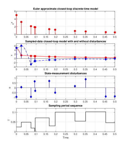
Figure 1: Evolution of the sampled-data system for the disturbance-free case (red solid line) and in the presence of state-measurement disturbances (blue dashed line) for a given sequence of sampling periods. The state of the approximate and exact discrete-time models is represented with stems in both cases.

First, we prove that $(\bar{F}^{Euler},\bar{F}^{e})$ is REPMC via Theorem 3.9. Assumptions 2.1 to 2.3 are easy to verify for the plant $\dot{x}=f(x,u)$ and control law $U(x,e,T)$. To prove conditions i) and ii), define $\phi\in\mathcal{K}_{\infty}$ via $\phi(s):=s^{9}+3s^{7}+3s^{5}$, then

$$\left|f(0,U(0,e,T))\right|=\frac{1}{2}\left|e^{9}+3e^{7}+3e^{5}\right|\leq|e|^{9}+3|e|^{7}+3|e|^{5}=\phi(|e|)$$

for all $T\in(0,1)$, thus i) holds. The function $f(x,U(x,e,T))$ is easily seen to be a multivariate polynomial in the variables $x,e,T$. Therefore, this function is locally Lipschitz in $x$, uniformly with respect to the other variables in compact sets and ii) holds. By Theorem 3.9, $(\bar{F}^{Euler},\bar{F}^{e})$ is REPC and by Lemma 3.7 also REPMC. By Theorem 3.5 then $\bar{F}^{e}$ is SE-ISS-VSR.

In order to illustrate the results we simulated the approximate Euler closed-loop model (used for control design) and the original sampled-data model (both with and without disturbances) from initial condition $x(0)=5$ for the same sequence of random sampling periods on a given interval. We considered the case where random continuous uniformly distributed state-measurment disturbances $e\in[-1,1]$ are present. The simulations in Figure 1 show the expected behaviour.

5 Conclusions

We have presented novel results that guarantee the semiglobal exponential input-to-state stability (SE-ISS-VSR) for discrete-time models of nonlinear nonuniformly sampled plants under state-measurement or actuation-error disturbances based on approximate discrete-time models. We have proved that under a multistep consistency property (REPMC) between two discrete-time models the SE-ISS-VSR property is carried over between models. We have shown that a much easier-to-verify one-step condition (REPC) is a transitive property and that it constitutes a sufficient condition for REPMC. Furthermore, we have proved that under mild boundedness and continuity conditions on the continuous-time model and the control law, any explicit and consistent Runge-Kutta (approximate) model is REPC with the exact discrete/time model and thus can be used for control design. We have provided an example of semiglobal exponential stabilization discrete-time design based on Runge-Kutta models.

Very recently, we proved that the simplest implicit Runge-Kutta model (backward Euler), is also REPC with the exact model [Vallarella et al., 2020]. We conjecture that this holds also for all implicit Runge-Kutta models and also for other types of well-known models. This is a topic for future work, as well as extending Theorem 3.9 to the case of dynamic controllers.

Appendix A Proof of Proposition 3.2

Let the REPC property define $\phi_{1}\in\mathcal{K}_{\infty}$ and $\phi_{2}\in\mathcal{K}_{\infty}$ for the the pairs $(\bar{F}^{a},\bar{F}^{b})$ and $(\bar{F}^{b},\bar{F}^{c})$, respectively. Suppose $M,E\geq 0$ given and let them generate $K_{1},T^{*,1}>0$, $\rho_{1}\in\mathcal{K}_{\infty}$ and $K_{2},T^{*,2}>0$, $\rho_{2}\in\mathcal{K}_{\infty}$ according to Definition 3.1 for the pairs $(\bar{F}^{a},\bar{F}^{b})$ and $(\bar{F}^{b},\bar{F}^{c})$, respectively. Consider $|x^{a}|,|x^{c}|\leq M$ and $|e|\leq E$ given. Define $K:=K_{1}$, $T^{*}:=\min\{T^{*,1},T^{*,2}\}$ and $\rho,\phi\in\mathcal{K}_{\infty}$ via $\rho:=\rho_{1}+\rho_{2}$ and $\phi:=\phi_{1}+\phi_{2}$. Thus we have

$$\left|\bar{F}^{a}(x^{a},e,T)-\bar{F}^{c}(x^{c},e,T)\right|$$

$$\leq\left|\bar{F}^{a}(x^{a},e,T)-\bar{F}^{b}(x^{c},e,T)\right|+\left|\bar{F}^{b}(x^{c},e,T)-\bar{F}^{c}(x^{c},e,T)\right|$$

$$\leq(1+K_{1}T)|x^{a}-x^{c}|+T\rho_{1}(T)\left(\max\{|x^{a}|,|x^{c}|\}+\phi_{1}(|e|)\right)$$

$$\qquad+(1+K_{2}T)|x^{c}-x^{c}|+T\rho_{2}(T)\left(\max\{|x^{c}|,|x^{c}|\}+\phi_{2}(|e|)\right)$$

$$\leq(1+KT)|x^{a}-x^{c}|+T\rho_{1}(T)\left(\max\{|x^{a}|,|x^{c}|\}+\phi(|e|)\right)$$

$$\qquad+T\rho_{2}(T)\left(\max\{|x^{a}|,|x^{c}|\}+\phi(|e|)\right)$$

$$\leq(1+KT)(|x^{a}-x^{c}|)+T\rho(T)(\max\{|x^{a}|,|x^{c}|\}+\phi(|e|)).$$ (23)

for all $|x^{a}|,|x^{c}|\leq M$, $|e|\leq E$ and $T\in(0,T^{*})$ and the pair $(\bar{F}^{a},\bar{F}^{c})$ is REPC.

$\hfill\blacksquare$

Appendix B Proof of Lemma 3.4

Consider $M_{a},E\geq 0$ and $\mathcal{T},\eta>0$ given. Since $\bar{F}^{a}$ is REPMC with $\bar{F}^{e}$ define $M_{e}:=(1+\eta)M_{a}+\phi(E)$ and generate $T^{*}:=T^{*}(M_{e},E,\mathcal{T},\eta)>0$ and function $\alpha:\mathbb{R}_{\geq 0}\times\mathbb{R}_{\geq 0}\rightarrow\mathbb{R}_{\geq 0}\cup\{\infty\}$ according to Definition 3.3. Define $T^{L}:=T^{*}$ and consider $\{T_{i}\}\in\Phi(T^{L})$ and $\|\{e_{i}\}\|\leq E$. Define $\Delta x_{k}:=x^{e}(k,\xi,\{e_{i}\},\{T_{i}\})-x^{a}(k,\xi,\{e_{i}\},\{T_{i}\})$. For $k=0$ we have

$$|\Delta x_{0}|:=|\xi-\xi|=0\leq\eta|\xi|+\phi(E).$$ (24)

We proceed by induction on $k$. Let $k\in\mathbb{N}_{0}$ be such that $\sum_{i=0}^{k-1}T_{i}\in[0,\mathcal{T}]$. Suppose that $|x^{a}(j,\xi,\{e_{i}\},\{T_{i}\})|\leq M_{a}$ and $|\Delta x_{j}|\leq\eta|\xi|+\phi(\sup_{0\leq i\leq j-1}|e_{i}|)$ for all $0\leq j\leq k$. Thus $|x^{e}(j,\xi,\{e_{i}\},\{T_{i}\})|\leq M_{a}+\eta|\xi|+\phi(\sup_{0\leq i\leq j-1}|e_{i}|)\leq M_{e}$ for all $0\leq j\leq k$. From (7) and (8) and noting that by causality $\Delta x_{k+1}$ cannot depend on future values of $e_{i}$ we have

$$|\Delta x_{k+1}|=|\bar{F}^{e}(x^{e}_{k},e_{k},T_{k})-\bar{F}^{a}(x^{a}_{k},e_{k},T_{k})|\leq\alpha(|\Delta x_{k}|,\{T_{i}\})$$

$$\leq\alpha^{k+1}(|\Delta x_{0}|,\{T_{i}\})=\alpha^{k+1}(0,\{T_{i}\})\leq\eta|\xi|+\phi\left(\sup_{0\leq i\leq k}|e_{i}|\right). \hfill\blacksquare$$

Appendix C Proof of Theorem 3.5

Let $K_{a},\lambda_{a}>0$, $\gamma_{a}\in\mathcal{K}_{\infty}$ and $T^{\star}(\cdot,\cdot)$ characterize the SE-ISS-VSR property of $x^{a}_{k}=\bar{F}^{a}(x^{a},e_{k},T_{k})$. Consider $M\geq 0$ and $E\geq 0$ given. Consider $\phi\in\mathcal{K}_{\infty}$ from i) and define $\hat{\gamma}\in\mathcal{K}_{\infty}$ via $\hat{\gamma}:=\gamma_{a}+\phi$. Let $\delta\in(0,1)$ and $\eta\in(0,\delta)$. Define $M_{a}:=K_{a}M+\frac{1}{1-\delta}\hat{\gamma}(E)$. Let $\mathcal{T}:=\frac{1}{\lambda_{a}}\ln{\frac{K_{a}}{\delta-\eta}}$. Define $\mathcal{T}_{1}:=\mathcal{T}+1$ and generate $T^{L}:=T^{L}(M_{a},E,\mathcal{T}_{1},\eta)$ according to Lemma 3.4. We have

$$|x^{a}_{k}|\leq K_{a}|\xi|\exp{\left(-\lambda_{a}\sum_{i=0}^{k-1}T_{i}\right)}+\gamma_{a}\left(\sup_{0\leq i\leq k-1}|e_{i}|\right)$$ (25)

for all $k\in\mathbb{N}_{0}$, $|\xi|\leq M_{a}$, $\{T_{i}\}\in\Phi(T^{\star}(M_{a},E))$ and $\|\{e_{i}\}\|\leq E$. Define $\bar{T}<\min\left\{1,T^{\star}(M_{a},E),T^{L}\right\}$. Consider $\{T_{i}\}\in\Phi(\bar{T})$. For every $k\in\mathbb{N}_{0}$ and $j\in\mathbb{N}$, define

$$s(k) :=\sup\left\{r\in\mathbb{N}_{0}:r\geq k+1,\sum_{i=k}^{r-1}T_{i}\leq\mathcal{T}_{1}\right\}\text{ and}$$ (26)

$$s^{j}(k) :=\overbrace{s(\ldots s(s}^{j}(k)))$$ (27)

Note that $s^{1}(k)\geq k+1$ for all $k\in\mathbb{N}_{0}$ because $\mathcal{T}_{1}>1$ and $T_{i}<1$ for all $i\in\mathbb{N}_{0}$. Also, $\sum_{i=k}^{s^{1}(k)-1}T_{i}>\mathcal{T}_{1}-\bar{T}>\mathcal{T}_{1}-1=\mathcal{T}$ holds for all $k\in\mathbb{N}_{0}$. For every $k,\ell\in\mathbb{N}_{0}$ with $k\geq\ell$ and $|\xi|\leq M_{a}$ define $\Delta x^{\xi}_{k,\ell}:=|x^{b}(k-\ell,\xi,\{e_{i+\ell}\},\{T_{i+\ell}\})-x^{a}(k-\ell,\xi,\{e_{i+\ell}\},\{T_{i+\ell}\})|$. Consider that $|\xi|\leq M$. Then $|x^{a}_{k}|\leq M_{a}$ for all $k\in\mathbb{N}_{0}$, $\{T_{i}\}\in\Phi(\bar{T})$ and $\|\{e_{i}\}\|\leq E$. From i), according to Lemma 3.4, for all $k\in\mathbb{N}_{0}$ for which $\sum_{i=0}^{k-1}\leq\mathcal{T}_{1}$ and $\{T_{i}\}\in\Phi(\bar{T})$ we have

$$|x^{b} (k,\xi,x\{e_{i}\},\{T_{i}\})|\leq|x^{a}(k,\xi,\{e_{i}\},\{T_{i}\})|+\left|\Delta x^{\xi}_{k,0}\right|$$

$$\leq K_{a}|\xi|\exp{\left(-\lambda_{a}\sum_{i=0}^{k-1}T_{i}\right)}+\gamma_{a}\left(\sup_{0\leq i\leq k-1}|e_{i}|\right)+\left|\Delta x^{\xi}_{k,0}\right|$$

$$\leq K_{a}|\xi|\exp{\left(-\lambda_{a}\sum_{i=0}^{k-1}T_{i}\right)}+\gamma_{a}\left(\sup_{0\leq i\leq k-1}|e_{i}|\right)+\eta|\xi|+\phi\left(\sup_{0\leq i\leq k-1}|e_{i}|\right)$$

$$\leq K_{a}|\xi|\left(\exp{\left(-\lambda_{a}\sum_{i=0}^{k-1}T_{i}\right)}+\frac{\eta}{K_{a}}\right)+\hat{\gamma}\left(\sup_{0\leq i\leq k-1}|e_{i}|\right).$$

For the sake of notation define $x^{b}_{s^{j}(0)}:=x^{b}(s^{j}(0),\xi,\{e_{i}\},\{T_{i}\})$. For instant $s^{1}(0)$ we have

$$|x^{b}_{s^{1}(0)}| \leq K_{a}|\xi|\left(\exp{\left(-\lambda_{a}\sum_{i=0}^{s^{1}(0)-1}T_{i}\right)}+\frac{\eta}{K_{a}}\right)+\hat{\gamma}\left(\sup_{0\leq i\leq s^{1}(0)-1}|e_{i}|\right)$$

$$\leq K_{a}|\xi|\left(\exp{\left(-\lambda_{a}\mathcal{T}\right)}+\frac{\eta}{K_{a}}\right)+\hat{\gamma}\left(\sup_{0\leq i\leq s^{1}(0)-1}|e_{i}|\right)$$

$$\leq K_{a}|\xi|\left(\frac{\delta-\eta}{K_{a}}+\frac{\eta}{K_{a}}\right)+\hat{\gamma}\left(\sup_{0\leq i\leq s^{1}(0)-1}|e_{i}|\right)$$

$$\leq\delta|\xi|+\hat{\gamma}\left(\sup_{0\leq i\leq s^{1}(0)-1}|e_{i}|\right)$$ (28)

$$\leq\delta M+\hat{\gamma}\left(E\right)\leq M_{a}$$

Note that for an initial condition such that $|x^{b}_{s^{j}(0)}|\leq M_{a}$ for some $j\in\mathbb{N}_{0}$ then, following the same reasoning that leads to (28), we can bound $|x^{b}_{s^{j+1}(0)}|$ as

$$|x^{b}_{s^{j+1}(0)}|\leq\delta|x^{b}_{s^{j}(0)}|+\hat{\gamma}\left(E\right).$$ (29)

Thus, we have $|x^{b}_{s^{j+1}(0)}|\leq\delta M_{a}+\hat{\gamma}(E)=\delta(K_{a}M+\frac{1}{1-\delta}\hat{\gamma}(E))+\hat{\gamma}(E)=\delta K_{a}M+(\frac{\delta}{1-\delta}+1)\hat{\gamma}(E))=\delta K_{a}M+\frac{1}{1-\delta}\hat{\gamma}(E)<M_{a}$. Thus $\left|x^{b}_{s^{j}(0)}\right|\leq M_{a}$ for all $j\in\mathbb{N}_{0}$. Then we can apply (28) iteratively to obtain

$$\left|x^{b}_{s^{j}(0)}\right| \leq\delta^{j}|\xi|+\hat{\gamma}\left(\sup_{0\leq i\leq s^{j}(0)-1}|e_{i}|\right)\sum_{i=0}^{j-1}\delta^{i}$$

$$=\exp{\left(-\lambda_{1}j\right)}|\xi|+\frac{1-\delta^{j}}{1-\delta}\hat{\gamma}\left(\sup_{0\leq i\leq s^{j}(0)-1}|e_{i}|\right)$$ (30)

where $\lambda_{1}:=\ln{\frac{1}{\delta}}>0$. Using the definition of $s^{j}(0)$ we have

$$-\lambda_{1}j=-\lambda_{1}j\frac{\mathcal{T}_{1}}{\mathcal{T}_{1}}\leq-\lambda_{1}\frac{\sum_{i=0}^{s^{j}(0)-1}T_{i}}{\mathcal{T}_{1}}=-\bar{\lambda}\sum_{i=0}^{s^{j}(0)-1}T_{i}$$ (31)

where $\bar{\lambda}:=\lambda_{1}/\mathcal{T}_{1}$. Using (31) on (30) and the fact that for $\delta\in(0,1)$ it holds that $\frac{1-\delta^{j}}{1-\delta}\leq\frac{1}{1-\delta}$ for all $j\in N_{0}$, we have

$$\left|x^{e}_{s^{j}(0)}\right|\leq\exp{\left(-\bar{\lambda}\sum_{i=0}^{s^{j}(0)-1}T_{i}\right)}|\xi|+\frac{1}{1-\delta}\hat{\gamma}\left(\sup_{0\leq i\leq s^{j}(0)-1}|e_{i}|\right).$$ (32)

Define $x^{b}_{k}(\xi):=x^{b}(k,\xi,\{e_{i}\},\{T_{i}\})$. From ii) and Lemma 3.4, for all $k\in[s^{j}(0),s^{j+1}(0)]$, we have that

$$\left|x^{b}_{k}(\xi)\right|=\left|x^{b}(k-s^{j}(0),x^{b}_{s^{j}(0)},\{e_{i+s^{j}(0)}\},\{T_{i+s^{j}(0)}\})\right|$$

$$\leq\left|x^{a}(k-s^{j}(0),x^{b}_{s^{j}(0)},\{e_{i+s^{j}(0)}\},\{T_{i+s^{j}(0)}\})\right|$$

$$\qquad+\big{|}x^{b}(k-s^{j}(0),x^{b}_{s^{j}(0)},\{e_{i+s^{j}(0)}\},\{T_{i+s^{j}(0)}\})$$

$$\qquad-x^{a}(k-s^{j}(0),x^{b}_{s^{j}(0)},\{e_{i+s^{j}(0)}\},\{T_{i+s^{j}(0)}\})\big{|}$$

$$\leq K_{a}\left|x^{b}_{s^{j}(0)}\right|+\gamma_{a}\left(\sup_{s^{j}(0)\leq i\leq k-1}|e_{i}|\right)+\eta\left|x^{b}_{s^{j}(0)}\right|+\phi\left(\sup_{s^{j}(0)\leq i\leq k-1}|e_{i}|\right)$$

$$\leq(K_{a}+\eta)\left|x^{b}_{s^{j}(0)}\right|+\hat{\gamma}\left(\sup_{s^{j}(0)\leq i\leq k-1}|e_{i}|\right).$$ (33)

Using (32) and (33), for all $k\in[s^{j}(0),s^{j+1}(0)]$, we have

$$|x^{b}_{k}(\xi)|\leq(K_{a}+\eta)\left|x^{b}_{s^{j}(0)}\right|+\hat{\gamma}\left(\sup_{s^{j}(0)\leq i\leq k-1}|e_{i}|\right)$$

$$\leq(K_{a}+\eta)\left(\exp{\left(-\bar{\lambda}\sum_{i=0}^{s^{j}(0)-1}T_{i}\right)}|\xi|+\frac{1}{1-\delta}\hat{\gamma}\left(\sup_{0\leq i\leq s^{j}(0)-1}|e_{i}|\right)\right)$$

$$\qquad+\hat{\gamma}\left(\sup_{s^{j}(0)\leq i\leq k-1}|e_{i}|\right)$$

$$\leq(K_{a}+\eta)\exp{\left(-\bar{\lambda}\sum_{i=0}^{s^{j}(0)-1}T_{i}\right)}|\xi|$$

$$\qquad+\left(\frac{(K_{a}+\eta)}{1-\delta}+1\right)\hat{\gamma}\left(\sup_{0\leq i\leq s^{j}(0)-1}|e_{i}|\right)$$

$$\leq(K_{a}+\eta)\exp{\left(-\bar{\lambda}\left(\sum_{i=0}^{k-1}T_{i}-\mathcal{T}_{1}\right)\right)}|\xi|+\gamma_{b}\left(\sup_{0\leq i\leq s^{j}(0)-1}|e_{i}|\right)$$

$$\leq(K_{a}+\eta)\exp{\left(\bar{\lambda}\mathcal{T}_{1}\right)}\exp{\left(-\bar{\lambda}\sum_{i=0}^{k-1}T_{i}\right)}|\xi|+\gamma_{b}\left(\sup_{0\leq i\leq s^{j}(0)-1}|e_{i}|\right)$$

$$\leq K_{b}\exp{\left(-\bar{\lambda}\sum_{i=0}^{k-1}T_{i}\right)}|\xi|+\gamma_{b}\left(\sup_{0\leq i\leq s^{j}(0)-1}|e_{i}|\right)$$

for all $k\in\mathbb{N}_{0}$, $|\xi|\leq M$ and $\{T_{i}\}\in\Phi(\bar{T}(M,E))$, where $K_{b}:=(K_{a}+\eta)\exp{\left(\bar{\lambda}\mathcal{T}_{1}\right)}$ $=(K_{a}+\eta)/\delta$ and $\gamma_{b}\in\mathcal{K}_{\infty}$ is defined via $\gamma_{b}:=\left(\frac{K_{a}+\eta}{1-\delta}+1\right)\hat{\gamma}$. $\hfill\blacksquare$

Appendix D Proof of Theorem 3.6

The proof copies the proof of 2. $\Rightarrow$ 1. of [Vallarella and Haimovich, 2018, Theorem 3.2] but keeps track of the changes introduced by the fact that $\alpha_{i}(s)=K_{i}s^{N}$ with $N>0$ and $K_{i}\geq 1$ for all $i\in\{1,2,3\}$.

Since the assumptions of condition 2. of [Vallarella and Haimovich, 2018, Theorem 3.2] are satisfied, then by the latter theorem we know that system (4) is S-ISS-VSR. The function $\alpha\in\mathcal{K}_{\infty}$ in [Vallarella and Haimovich, 2018, eq.(28)] results $\alpha(s):=\alpha_{3}\circ\alpha_{2}^{-1}(s)=\tilde{\lambda}s$ where $\tilde{\lambda}:=\frac{K_{3}}{K_{2}^{1/N}}$. Therefore, the right-hand side of inequality [Vallarella and Haimovich, 2018, eq.(32)] is linear in $y$. It then follows that the function $\beta_{1}\in\mathcal{KL}$ in [Vallarella and Haimovich, 2018, eq.(33)] is given by $\beta_{1}(s,t)=s\exp{\left(-\tilde{\lambda}t\right)}$. Then, the function $\beta\in\mathcal{KL}$ in [Vallarella and Haimovich, 2018, eq.(35)] defined via $\beta(s,t):=\alpha_{1}^{-1}(2\beta_{1}(\alpha_{2}(s),t))$ becomes $\beta(s,t)=Ks\exp{(-\lambda t)}$ where $K:=\frac{2K_{2}}{K_{1}^{1/N}}$ and $\lambda:=\frac{\tilde{\lambda}}{N}$. Since this function $\beta$ characterizes the S-ISS-VSR property, it follows from Definition 2.5 that system (4) is SE-ISS-VSR. $\hfill\blacksquare$

Appendix E Proof of Lemma 3.8

Consider $\tilde{\mathcal{X}}\subset\mathbb{R}^{n}$ and $\mathcal{U}\subset\mathbb{R}^{m}$ given and let $\phi_{u}(t,\xi):=F^{e}(\xi,u,t)$ be the unique solution of (1) that begins from initial condition $\xi\in\tilde{\mathcal{X}}$ at $t_{0}=0$ and has a constant input $u\in\mathcal{U}$. Then

$$\phi_{u}(t,\xi)=\xi+\int_{0}^{t}f(\phi_{u}(\tau,\xi),u)d\tau.$$ (34)

Define $C_{u}:=\max_{u\in\mathcal{U}}\{|u|\}$, $R:=\max\{1,\max_{x\in\tilde{\mathcal{X}}}|x|\}$ and $\hat{\mathcal{X}}:=\{x\in\mathbb{R}^{n}:|x|\leq 2R\}$ and generate $C_{f}=C_{f}(2R,C_{u})$ from Assumption 2.2. Then

$$|\phi_{u}(t,\xi)|\leq|\xi|+\int_{0}^{t}|f(\phi_{u}(\tau,\xi),u)|d\tau\leq R+C_{f}t.$$

for all $t\in(0,\bar{T})$ with $\bar{T}:=R/C_{f}$. Define $\mathcal{X}:=\{x:|x|\leq R+C_{f}\bar{T}\}$ and $\tilde{L}:=\tilde{L}(\mathcal{X},\mathcal{U})$ from Assumption 2.1. The error between the solutions of the exact model and the Euler approximate model after one step of duration $T\in(0,\bar{T})$ from initial condition $x^{e}_{0}=x^{a}_{0}=\xi$ with $\xi\in\tilde{\mathcal{X}}$ and input $u\in\mathcal{U}$ results

$$\vartheta(T): =F^{e}(\xi,u,T)-F^{Euler}(\xi,u,T)$$

$$=\xi+\left(\int_{0}^{T}f(\phi_{u}(\tau,\xi),u)d\tau\right)-\xi-Tf(\xi,u)$$

$$=\int_{0}^{T}f(\phi_{u}(\tau,\xi),u)d\tau-Tf(\xi,u)$$

$$=\int_{0}^{T}f(\phi_{u}(\tau,\xi),u)-f(\xi,u)d\tau.$$ (35)

Taking the norm on both sides of (35) we have

$$|\vartheta(T)|=\left|\int_{0}^{T}f(\phi_{u}(\tau,\xi),u)-f(\xi,u)d\tau\right|$$

$$\leq\int_{0}^{T}\left|f(\phi_{u}(\tau,\xi),u)-f(\xi,u)\right|d\tau\leq\tilde{L}\int_{0}^{T}|\phi_{u}(\tau,\xi)-\xi|d\tau$$

$$=\tilde{L}\int_{0}^{T}\left|F^{e}(\xi,u,\tau)-F^{Euler}(\xi,u,\tau)+\tau f(\xi,u)\right|d\tau$$

$$\leq\tilde{L}\int_{0}^{T}|\vartheta(\tau)|d\tau+\tilde{L}\int_{0}^{T}\tau|f(\xi,u)|d\tau$$

$$\leq\tilde{L}\int_{0}^{T}|\vartheta(\tau)|d\tau+\tilde{L}\frac{T^{2}}{2}|f(\xi,u)|$$ (36)

From (36), by Gronwall’s inequality, we can bound the error as $|\vartheta(T)|\leq\tilde{L}\frac{T^{2}}{2}|f(\xi,u)|e^{\tilde{L}T}$ for all $T\in[0,\bar{T})$. Defining $\bar{L}:=\frac{1}{2}\tilde{L}e^{\tilde{L}\bar{T}}$ we have that

$$|F^{e}(\xi,u,T)-F^{Euler}(\xi,u,T)|\leq\bar{L}T^{2}|f(\xi,u)|$$ (37)

for all $\xi\in\mathcal{X}$, $u\in\mathcal{U}$ and $T\in(0,\bar{T})$. $\hfill\blacksquare$

Appendix F Proof of Theorem 3.9

We will establish that $(\bar{F}^{RK},\bar{F}^{e})$ is REPC by showing that both $(\bar{F}^{Euler},\bar{F}^{e})$ and $(\bar{F}^{RK},\bar{F}^{Euler})$ are REPC and using the fact that REPC is transitive.

Consider $M,E\geq 0$ given and let them generate $K,T^{ii}>0$ from ii) and $T^{i}>0$ from i). Let $M,E$ generate $C_{u},T^{u}>0$ from Assumption 2.3. Define $\mathcal{X}:=\{x\in\mathbb{R}^{n}:|x|\leq M\}$ and $\mathcal{U}:=\{u\in\mathbb{R}^{m}:|u|\leq C_{u}\}$.

Claim 1.

$(\bar{F}^{Euler},\bar{F}^{e})$ is REPC.

Proof of Claim 1: From Assumptions 2.1 and 2.2, the conditions of Lemma 3.8 hold. Let $\mathcal{X}$ and $\mathcal{U}$ generate $\bar{L},\bar{T}>0$ from Lemma 3.8, so that the open-loop condition (13) holds for all $x\in\mathcal{X}$, $u\in\mathcal{U}$ and $T\in(0,\bar{T})$. Define $T^{o}:=\min\{\bar{T},T^{u},T^{i},T^{ii}\}$, $\bar{K}:=\max\{K,1\}$ and $\rho\in\mathcal{K}_{\infty}$ via $\rho(s):=\bar{K}\bar{L}s$. For all $|x^{e}|,|x^{a}|\leq M$, $|e|\leq E$ and $T\in(0,T^{o})$ we have

$$|\bar{F}^{e}(x^{e},e,T)-\bar{F}^{Euler}(x^{a},e,T)|$$

$$\leq|F^{e}(x^{e},U(x^{e},e,T),T)-F^{Euler}(x^{e},U(x^{e},e,T),T)|$$

$$+|F^{Euler}(x^{e},U(x^{e},e,T),T)-F^{Euler}(x^{a},U(x^{a},e,T),T)|$$

$$\leq|F^{e}(x^{e},U(x^{e},e,T),T)-F^{Euler}(x^{e},U(x^{e},e,T),T)|$$

$$+|x^{e}-x^{a}|+T|f(x^{e},U(x^{e},e,T))-f(x^{a},U(x^{a},e,T))|$$ (38)

$$\leq(1+KT)|x^{e}-x^{a}|+\bar{L}T^{2}|f(x^{e},U(x^{e},e,T))|$$ (39)

$$\leq(1+KT)|x^{e}-x^{a}|$$

$$+\bar{L}T^{2}(|f(x^{e},U(x^{e},e,T))-f(0,U(0,e,T))|+|f(0,U(0,e,T))|)$$

$$\leq(1+KT)|x^{e}-x^{a}|+\bar{L}T^{2}\left(K|x^{e}|+\phi(|e|)\right)$$ (40)

$$\leq(1+KT)|x^{e}-x^{a}|+T\rho(T)(|x^{e}|+\phi(|e|)).$$ (41)

In (38) we have used the definition of the Euler approximation. In (39) we have used (16) from ii) and (13) from Lemma 3.8. In (40) we have used (15) from i) and (16) from ii). Note that $\phi\in\mathcal{K}_{\infty}$ is given by i) and hence does not depend on $M$ or $E$. Thus, (3.1) holds and $(\bar{F}^{Euler},\bar{F}^{e})$ is REPC. $\circ$

Claim 2.

$(\bar{F}^{RK},\bar{F}^{Euler})$ is REPC.

Proof of Claim 2: For the sake of notation, define $\bar{f}(x,e,T):=f(x,U(x,e,T))$. Employing the definitions of the Euler and Runge-Kutta models, we have

$$\big{|}\bar{F}^{Euler}(x,e,T) -\bar{F}^{RK}(z,e,T)\big{|}$$

$$\leq|x-z|+T\left|\bar{f}(x,e,T)-\sum_{i=1}^{s}b_{i}\bar{f}(y_{i},e,T)\right|$$

Adding and subtracting $\left(\sum_{i=j}^{s}b_{i}\right)\bar{f}(y_{j-1},e,T)$, for $j=2,\ldots,s$, and operating, we reach

$$\big{|}\bar{F}^{Euler}(x,e,T)-\bar{F}^{RK}(z,e,T)\big{|}\leq|x-z|$$

$$+T\Bigg{|}\bar{f}(x,e,T)\ -\left[\sum_{j=2}^{s}\left(\sum_{i=j}^{s}b_{i}\right)\big{[}\bar{f}(y_{j},e,T)-\bar{f}(y_{j-1},e,T)\right]$$

$$+\left(\sum_{i=1}^{s}b_{i}\right)\bar{f}(y_{1},e,T)\big{]}\Bigg{|}.$$

Taking into account that $\sum_{i=1}^{s}b_{i}=1$ and that $y_{1}=z$, then

$$\big{|}\bar{F}^{Euler}(x,e,T)-\bar{F}^{RK}(z,e,T)\big{|}\leq|x-z|$$ (42)

$$+T\left|\bar{f}(x,e,T)-\bar{f}(z,e,T)\right|+TB\sum_{j=2}^{s}\left|\bar{f}(y_{j},e,T)-\bar{f}(y_{j-1},e,T)\right|$$

with $B:=\sum_{i=2}^{s}|b_{i}|$. Define $T^{\#}:=\min\{1,T^{u},T^{iv},T^{v}\}>0$ and $A:=2\max_{i=2,\ldots,s,j=1,\ldots,i-1}|a_{ij}|$. Consider $|x|\leq M$, $|e|\leq E$, and $T\in(0,T^{\#})$. From (14) we have

$$|y_{i}|\leq|y_{1}|+T^{\#}\sum_{j=1}^{i-1}|a_{ij}|\left|\bar{f}(y_{j},e,T)\right|$$

$$\leq|x|+T^{\#}A\sum_{j=1}^{s-1}\left|f(y_{j},U(y_{j},e,T))\right|,\quad\text{for }i=2,\ldots,s.$$ (43)

Define $M_{1}:=M$ and recursively for $i=2,\ldots,s$,

$$M_{i}:=M_{i-1}+(s-1)T^{\#}AC_{f}\left(M_{i-1},C_{u}(M_{i-1},E)\right),$$

where $C_{f}(\cdot,\cdot)$ and $C_{u}(\cdot,\cdot)$ are given by Assumptions 2.2 and 2.3. With these definitions, it follows that $|y_{i}|\leq M_{s}\text{ for all }1\leq i\leq s$. Define $T^{*}:=\min\{1,T^{\#},T^{u}(M_{s},E),T^{iv}(E),T^{v}(M_{s},E)\}$. and $K_{s}:=\max\{K(M_{s},E),1\}$. For $T\in(0,T^{*})$, it follows that

$$\left|\bar{f}(y_{1},e,T)\right| \leq\left|\bar{f}(y_{1},e,T)-\bar{f}(0,e,T)\right|+\left|\bar{f}(0,e,T)\right|$$

$$\leq K_{s}|y_{1}|+\phi(|e|)$$

and for $i=2,\ldots,s$

$$\left|\bar{f}(y_{i},e,T)\right|$$

$$\leq|f(y_{i},U(y_{i},e,T))-f(0,U(0,e,T)|+|f(0,U(0,e,T))|$$

$$\leq K_{s}|y_{i}|+\phi(|e|)\leq K_{s}\left|y_{1}+T\sum_{j=1}^{i-1}a_{ij}\bar{f}(y_{j},e,T)\right|+\phi(|e|)$$

$$\leq K_{s}|y_{1}|+K_{s}T\left|\sum_{j=1}^{i-1}a_{ij}\bar{f}(y_{j},e,T)\right|+\phi(|e|)$$

$$\leq K_{s}|y_{1}|+\phi(|e|)+K_{s}AT\sum_{j=1}^{i-1}\left|\bar{f}(y_{j},e,T)\right|.$$ (44)

Using (44) recursively yields

$$\left|\bar{f}(y_{i},e,T)\right| \leq\left[K_{s}|y_{1}|+\phi(|e|)\right]\sum_{j=0}^{i-1}(K_{s}AT)^{j}$$

$$\leq C\left(|y_{1}|+\phi(|e|)\right),\quad\text{for }i=1,\ldots,s,$$ (45)

where we have used the fact that $K_{s}\geq 1$ and defined $C:=K_{s}\sum_{j=0}^{s-1}(K_{s}AT^{*})^{j}$. From (42) and ii), then provided $T\in(0,T^{*})$, we have

$$\big{|}\bar{F}^{Euler}(x,e,T)-\bar{F}^{RK}(z,e,T)\big{|}$$

$$\leq(1+KT)|x-z|+TBK_{s}\sum_{j=2}^{s}\left|y_{j}-y_{j-1}\right|.$$ (46)

Using (14) and defining $a_{ij}:=0$ for $j\geq i$, we have

$$|y_{i}-y_{i+1}| =\left|T\sum_{j=1}^{s}(a_{ij}-a_{(i+1)j})\bar{f}(y_{j},e,T)\right|$$

$$\leq TA\sum_{j=1}^{s}|\bar{f}(y_{j},e,T)|\quad\text{for }i=1,\ldots,s-1.$$ (47)

Combining (47) and (46), then

$$|\bar{F}^{Euler}(x,e,T)-\bar{F}^{RK}(z,e,T)|$$

$$\leq(1+KT)|x-z|+(s-1)ABK_{s}T^{2}\sum_{j=1}^{s}\left|\bar{f}(y_{j},e,T)\right|$$ (48)

Using (45) in (48) we obtain, for all $|x|,|z|\leq M$, $|e|\leq E$ and $T\in(0,T^{*})$

$$|\bar{F}^{Euler}(x,e,T)-\bar{F}^{RK}(z,e,T)|$$

$$\leq(1+KT)|x-z|+(s-1)ABK_{s}T^{2}C\sum_{j=1}^{s}\left(|y_{1}|+\phi(|e|)\right)$$

$$\leq(1+KT)|x-z|+T\rho(T)\left(|z|+\phi(|e|)\right)$$

where $\rho\in\mathcal{K}_{\infty}$ is defined via $\rho(T):=(s-1)sABCK_{s}T$. Note that $\phi\in\mathcal{K}_{\infty}$ is given by i) and hence does not depend on $M$ or $E$. Thus, (3.1) holds and $(\bar{F}^{Euler},\bar{F}^{RK})$ is REPC. $\circ$

According with Claim 1 and Claim 2, by Proposition 3.2 then the pair $(\bar{F}^{RK},\bar{F}^{e})$ is REPC. $\hfill\blacksquare$

Appendix G Proof of Lemma 3.11

Consider $M,E\geq 0$ given and let the S-ISS-VSR property generate the bound (5) and $T^{\star}(M,E)$. Given some $k\in\mathbb{N}_{0}$, the evolution of the sampled-data system between any consecutive samples $x_{k}$ and $x_{k+1}$ of the continuous-time solution that begins from initial condition $|x_{0}|\leq M$ with $\|\{e_{i}\}\|\leq E$ and $\{T_{i}\}\in\Phi(T^{\star})$ is given by $x(t_{k}+t)=\bar{F}^{e}(x_{k},e_{k},t)$, thus

$$x(t_{k}+t)=x_{k}+\int_{0}^{t}f\left(\bar{F}^{e}(x_{k},e_{k},s),U(x_{k},e_{k},T_{k})\right)ds$$ (49)

for all $t\in[0,T_{k}]$. Define $R:=\beta(M,0)+\gamma(E)$ from Definition 2.5, then $|x_{k}|\leq R$ for all $k\in\mathbb{N}_{0}$. From Assumption 2.3 we have that $|U(x,e,T)|\leq C_{u}(|x|,|e|)$ for all $|x|\leq R$, $|e|\leq E$ and $T\in(0,T^{u}(R,E))$. Define $C(|x|,|e|):=C_{f}(2|x|,C_{u}(|x|,|e|))$ with $C_{f}$ from Assumption 2.2, and $\bar{T}(M,E):=\min\left\{T^{\star},T^{u},\frac{R}{C(R,E)}\right\}$. Next, we will prove that $|x(t_{k}+t)|\leq 2R$ for all $t\in[0,\bar{T}]$. Let $|x_{k}|\leq R$, $|e_{k}|\leq E$ and define

$$\tau:=\inf\left\{t>0:\left|F^{e}(x_{k},U(x_{k},e_{k},T_{k}),t)\right|\geq 2R\right\}.$$ (50)

Due to $F^{e}(x_{k},U(x_{k},e_{k},T_{k}),0)=x_{k}$ and the continuity of $F^{e}(x_{k},U(x_{k},e_{k},T_{k}),\cdot)$ we have $\tau>0$ for all $T_{k}\in[0,\bar{T}]$. For a contradiction, suppose that $\tau<\bar{T}$ for some $T_{k}\in[0,\bar{T}]$. From continuity and (50), it follows that $\left|F^{e}(x_{k},U(x_{k},e_{k},T_{k}),\tau)\right|=2R$ and $\left|F^{e}(x_{k},U(x_{k},e_{k},T_{k}),t)\right|<2R$ for all $t\in[0,\tau)$. Thus,

$$\left|F^{e}(x_{k},U(x_{k},e_{k},T_{k}),\tau)\right|$$

$$\leq|x_{k}|+\int_{0}^{\tau}\left|f\left(F^{e}(x_{k},U(x_{k},e_{k},T_{k}),s),U(x_{k},e_{k},T_{k})\right)\right|ds$$

$$<R+C(R,E)\bar{T}\leq 2R$$ (51)

The strict inequality in (51) contradicts $\left|F^{e}(x_{k},U(x_{k},e_{k},T_{k}),\tau)\right|=2R$. Therefore, $\tau\geq\bar{T}$. From (49), (51) and (5), then for all $k\in\mathbb{N}_{0}$, $\{T_{i}\}\in\Phi(\bar{T})$, $|x_{0}|\leq M$ and $\|\{e_{i}\}\|\leq E$, we have

$$\left|x(t_{k}+t)\right| \leq\beta\left(|x_{0}|,\sum_{i=0}^{k-1}T_{i}\right)+\gamma\left(\sup_{0\leq i\leq k-1}|e_{i}|\right)+C(R,E)t$$ (52)

for all $t\in[0,T_{k}]$.

References

- Abdelrahim et al. [2017] Abdelrahim, M., Postoyan, R., Daafouz, J., Nešić, D., 2017. Robust event-triggered output feedback controllers for nonlinear systems. Automatica 75, 96 – 108.
- Anta and Tabuada [2010] Anta, A., Tabuada, P., 2010. To sample or not to sample: Self-triggered control for nonlinear systems. IEEE Transactions on Automatic Control. 55, 2030–2042.
- Arcak and Nešić [2004] Arcak, M., Nešić, D., 2004. A framework for nonlinear sampled-data observer design via approximate discrete-time models and emulation. Automatica. 40, 1931–1938.
- Beikzadeh and Marquez [2015] Beikzadeh, H., Marquez, H.J., 2015. Multirate output feedback control of nonlinear networked control systems. IEEE Transactions on Automatic Control. 60, 1939–1944.
- Beikzadeh and Marquez [2016] Beikzadeh, H., Marquez, H.J., 2016. Input-to-error stable observer for nonlinear sampled-data systems with application to one-sided Lipschitz systems. Automatica. 67, 1–7.
- Di Ferdinando and Pepe [2017] Di Ferdinando, M., Pepe, P., 2017. Robustification of sample-and-hold stabilizers for control-affine time-delay systems. Automatica. 83, 141–154.
- Di Ferdinando and Pepe [2019] Di Ferdinando, M., Pepe, P., 2019. Sampled-data emulation of dynamic output feedback controllers for nonlinear time-delay systems. Automatica. 99, 120–131.
- Di Ferdinando et al. [2019] Di Ferdinando, M., Pepe, P., Fridman, E., 2019. Exponential input-to-state stability of globally Lipschitz time-delay systems under sampled-data noisy output feedback and actuation disturbances. International Journal of Control. 0, 1–11.
- Karafyllis and Kravaris [2009] Karafyllis, I., Kravaris, C., 2009. Global stability results for systems under sampled-data control. International Journal of Robust and Nonlinear Control. 19, 1105–1128.
- Lin [2020] Lin, W., 2020. When is a nonlinear system semiglobally asymptotically stabilizable by digital feedback? IEEE Transactions on Automatic Control 65, 4584–4599.
- Liu et al. [2008] Liu, X., Marquez, H.J., Lin, Y., 2008. Input-to-state stabilization for nonlinear dual-rate sampled-data systems via approximate discrete-time model. Automatica. 44, 3157–3161.
- Monaco and Normand-Cyrot [2007] Monaco, S., Normand-Cyrot, D., 2007. Advanced tools for nonlinear sampled-data systems’ analysis and control. European Journal of Control 13, 221–241.
- Nešić et al. [1999] Nešić, D., A. R. Teel, Kokotović, P.V., 1999. Sufficient conditions for stabilization of sampled-data nonlinear systems via discrete-time approximations. Systems & Control Letters. 38, 259–270.
- Nešić and Laila [2002] Nešić, D., Laila, D.S., 2002. A note on input-to-state stabilization for nonlinear sampled-data systems. IEEE Transactions on Automatic Control. 47, 1153–1158.
- Nešić et al. [2009] Nešić, D., Loría, A., Panteley, E., Teel, A.R., 2009. On stability of sets for sampled-data nonlinear inclusions via their approximate discrete-time models and summability criteria. SIAM Journal on Control and Optimization. 48, 1888–1913.
- Nešić and Teel [2004] Nešić, D., Teel, A.R., 2004. A framework for stabilization of nonlinear sampled-data systems based on their approximate discrete-time models. IEEE Transactions on Automatic Control. 49, 1103–1122.
- Nešić et al. [2009] Nešić, D., Teel, A.R., Carnevale, D., 2009. Explicit computation of the sampling period in emulation of controllers for nonlinear sampled-data systems. IEEE Transactions on Automatic Control 54, 619–624.
- Polushin and Marquez [2004] Polushin, I.G., Marquez, H.J., 2004. Multirate versions of sampled-data stabilization of nonlinear systems. Automatica 40, 1035 – 1041.
- Postoyan and Nešić [2012] Postoyan, R., Nešić, D., 2012. A framework for the observer design for networked control systems. IEEE Transactions on Automatic Control. 57, 1309–1314.
- Stuart and Humphries [1996] Stuart, A., Humphries, A., 1996. Dynamical Systems and numerical analysis. Cambridge University Press: NY.
- Vallarella et al. [2020] Vallarella, A.J., Cardone, P., Haimovich, H., 2020. On the use of backward euler for sampled-data control design, in: 27 Congreso Argentino de Control Automático (AADECA), Buenos Aires, Argentina. pp. 485–490.
- Vallarella and Haimovich [2018] Vallarella, A.J., Haimovich, H., 2018. Characterization of semiglobal stability properties for discrete-time models of non-uniformly sampled nonlinear systems. Systems & Control Letters. 122, 60 – 66. doi:https://doi.org/10.1016/j.sysconle.2018.10.005.
- Vallarella and Haimovich [2019] Vallarella, A.J., Haimovich, H., 2019. State measurement error-to-state stability results based on approximate discrete-time models. IEEE Transactions on Automatic Control. 64, 3308–3315. doi:10.1109/TAC.2018.2874669.
- van de Wouw et al. [2012] van de Wouw, N., Nešić, D., Heemels, W.P.M.H., 2012. A discrete-time framework for stability analysis of nonlinear networked control systems. Automatica. 48, 1144–1153.
- Yuz and Goodwin [2014] Yuz, J.I., Goodwin, G.C., 2014. Sampled-data models for linear and nonlinear systems. Springer.
- Zeng et al. [2017] Zeng, C., Liang, S., Xiang, S., 2017. A novel condition for stable nonlinear sampled-data models using higher-order discretized approximations with zero dynamics. ISA Transactions. 68, 73–81.
- Üstüntürk [2012] Üstüntürk, A., 2012. Output feedback stabilization of nonlinear dual-rate sampled-data systems via an approximate discrete-time model. Automatica. 48, 1796–1802.