Abstract

While modern large-scale datasets often consist of heterogeneous subpopulations—for example, multiple demographic groups or multiple text corpora—the standard practice of minimizing average loss fails to guarantee uniformly low losses across all subpopulations. We propose a convex procedure that controls the worst-case performance over all subpopulations of a given size. Our procedure comes with finite-sample (nonparametric) convergence guarantees on the worst-off subpopulation. Empirically, we observe on lexical similarity, wine quality, and recidivism prediction tasks that our worst-case procedure learns models that do well against unseen subpopulations.

1 Introduction

When we train models over heterogeneous data, a basic goal is to train models that perform uniformly well across all subpopulations instead of just on average. For example, in natural language processing (NLP), large-scale corpora often consist of data from multiple domains, each domain varying in difficulty and frequently containing large proportions of easy examples [21]. Standard approaches optimize average performance, however, and yield models that accurately predict easy examples but sacrifice predictive performance on hard subpopulations [62].

The growing use of machine learning systems in socioeconomic decision-making problems, such as loan-servicing and recidivism prediction, highlights the importance of models that perform well over different demographic groups [6]. In the face of this need, a number of authors observe that optimizing average performance often yields models that perform poorly on minority subpopulations [3, 36, 41, 17, 66, 76]. When datasets contain demographic information, a natural approach is to optimize worst-case group loss or equalize losses over groups. But in many tasks—such as language identification or video analysis [76, 17]—privacy concerns preclude recording demographic or other sensitive information, limiting the applicability of methods that require knowledge of demographic identities. For example, lenders in the United States are prohibited from asking loan applicants for racial information unless it is to demonstrate compliance with anti-discrimination regulation [20, 22].

To address these challenges, we seek models that perform well on each subpopulation rather than those that achieve good (average) performance by focusing on the easy examples and domains. Thus, in this paper we develop procedures that control performance over all large enough subpopulations, agnostic to the distribution of each subpopulation. We study a worst-case formulation over large enough subpopulations in the data, providing procedures that automatically focus on the difficult subsets of the dataset. Our procedure guarantees a uniform level of performance across subpopulations by hedging against unseen covariate shifts, potentially even in the presence of confounding.

In classical statistical learning and prediction problems, we wish to predict a target $Y\in\mathcal{Y}$ from a covariate vector $X\in\mathcal{X}\subset\mathbb{R}^{d}$ drawn from an underlying population $(X,Y)\sim P$, measuring performance of a predictor $\theta$ via the loss $\ell:\Theta\times(\mathcal{X}\times\mathcal{Y})\to\mathbb{R}_{+}$. The standard approach is to minimize the population expectation $\mathbb{E}_{P}[\ell(\theta;(X,Y))]$. In contrast, we consider an elaborated setting in which the observed data comes from a mixture model, and we evaluate model losses on a component (subpopulation) from this mixture. More precisely, we assume that for some mixing proportion $\alpha\in(0,1)$, the data $X$ are marginally distributed as $X\sim P_{X}:=\alpha Q_{0}+(1-\alpha)Q_{1}$, while the subpopulations $Q_{0}$ and $Q_{1}$ are unknown. The classical formulation does little to ensure equitable performance for data $X$ from both $Q_{0}$ and $Q_{1}$, especially for small $\alpha$. Thus for a fixed conditional distribution $P_{Y\mid X}$, we instead seek $\theta\in\Theta$ that minimizes the expected loss under the latent subpopulation $Q_{0}$

$$\mathop{\rm minimize}_{\theta\in\Theta}~{}\mathbb{E}_{X\sim Q_{0}}[\mathbb{E}[\ell(\theta;(X,Y))\mid X]].$$ (1)

We call this loss minimization under mixture covariate shifts.

As the latent mixture weight and components are unknown, it is impossible to compute the loss (1) from observed data. Thus, we postulate a lower bound $\alpha_{0}\in(0,\frac{1}{2})$ on the subpopulation proportion $\alpha$ and consider the set of potential minority subpopulations

$$\mathcal{P}_{\alpha_{0},X}:=\left\{Q_{0}:P_{X}=\alpha Q_{0}+(1-\alpha)Q_{1}~{}~{}\mbox{for some}~{}\alpha\geq\alpha_{0}~{}\mbox{and distribution}~{}Q_{1}~{}\mbox{on}~{}\mathcal{X}\right\}.$$

Concretely, our goal is to minimize worst-case subpopulation risk $\mathcal{R}$,

$$\mathop{\rm minimize}_{\theta\in\Theta}\left\{\mathcal{R}(\theta):=\sup_{Q_{0}\in\mathcal{P}_{\alpha_{0},X}}\underset{X\sim Q_{0}}{\mathbb{E}}[\mathbb{E}[\ell(\theta;(X,Y))\mid X]]\right\}.$$ (2)

The worst-case formulation (2) is a distributionally robust optimization (DRO) problem [9, 70] where we consider the worst-case loss over mixture covariate shifts $Q_{0}\in\mathcal{P}_{\alpha_{0},X}$, and we term the methodology we develop around this formulation marginal distributionally robust optimization, as we seek robustness only to shifts in the marginals over the covariates $X$. For datasets with heterogeneous subpopulations (e.g. natural language processing corpora), the worst-case subpopulation corresponds to a group that is “hard” under the current model $\theta$. As we detail in the related work section, the approach (2) has connections with covariate shift problems, distributional robustness, fairness, and causal inference. In particular, the dual form of (2) corresponds to the conditional-value-at-risk (CVaR) of the conditional risk $\mathbb{E}[\ell(\theta;(X,Y))\mid X]$.

In some instances, the worst-case subpopulation (2) may be too conservative; the distribution of $X$ may shift only on some components, or we may only care to achieve uniform performance across one variable. As an example, popular computer-vision datasets draw images mostly from western Europe and the United States [68], but one may wish for models that perform uniformly well over different geographic locations. In such cases, when one wishes to consider distributional shifts only on a subset of variables $X_{1}$ (e.g. geographic location) of the covariate vector $X=(X_{1},X_{2})$, we may simply redefine $X$ as $X_{1}$, and $Y$ as $(X_{2},Y)$ in the problem (2). All of our subsequent discussion generalizes to such scenarios.

On the other hand, because of confounding, the assumption that the conditional distribution $P_{Y\mid X}$ does not change across groups may be too optimistic. While the assumption is appropriate for machine learning tasks where human annotators use $X$ to generate the label $Y$, many problems include unmeasured confounding variables that affect the label $Y$ and vary across subpopulations. For example, in a recidivism prediction task, the feature $X$ may be the type of crime, the label $Y$ represents re-offending, and the subgroup may be race; without measuring unobserved variables, such as income or location, $P_{Y\mid X}$ is likely to differ between groups. To address this issue, in Section B we generalize our proposed worst-case loss (2) to incorporate worst-case confounding shifts, providing finite-sample upper bounds on worst-case loss whose tightness depends on the effect of the unmeasured confounders on the conditional risk $\mathbb{E}[\ell(\theta;(X,Y))\mid X]$.

1.1 Overview of results

In the rest of the paper, we construct a tractable finite sample approximation to the worst-case problem (2), and show that it allows learning models $\theta\in\Theta$ that perform uniformly well over subpopulations. Our starting point is the duality result (see Section 2.1)

$$\mathcal{R}(\theta) :=\sup_{Q_{0}\in\mathcal{P}_{\alpha_{0},X}}\mathop{\mathbb{E}}_{X\sim Q_{0}}[\mathbb{E}[\ell(\theta;(X,Y))\mid X]]=\inf_{\eta}\left\{\frac{1}{\alpha_{0}}\mathop{\mathbb{E}}_{X\sim P_{X}}[\left({\mathbb{E}[\ell(\theta;(X,Y))\mid X]-\eta}\right)_{+}]+\eta\right\}.$$

For convex losses, the dual form yields a single convex loss minimization in the variables $(\theta,\eta)$ for minimizing $\mathcal{R}(\theta)$. When we (approximately) know the conditional risk $\mathbb{E}[\ell(\theta;(X,Y))\mid X]$—for example, when we have access to replicate observations $Y$ for each $X$—it is reasonably straightforward to develop estimators for the risk (2) (see Section 2.2).

Estimating the conditional risk via replication is infeasible in scenarios in which $X$ corresponds to a unique individual (similar to issues in estimation of conditional treatment effects [44]). Alternative procedures that depend on parametric assumptions on the family of conditional risks $\mathbb{E}[\ell(\theta;X,Y)\mid X]$ for all $\theta\in\Theta$ are restrictive, as we study learning problems over a flexible class of machine learning models $\theta\in\Theta$ (e.g., random forests, gradient boosted decision trees, kernel methods, neural networks). In this work, we instead consider a scalable nonparametric approach involving the variational representation

$$\mathbb{E}[\left({\mathbb{E}[\ell(\theta;(X,Y))\mid X]-\eta}\right)_{+}]=\sup_{h:\mathcal{X}\to[0,1]}\mathbb{E}_{P}[h(X)(\ell(\theta;(X,Y))-\eta)].$$ (3)

As the space $\{h:\mathcal{X}\to[0,1]\}$ is too large to effectively estimate the quantity (3), we consider approximations via easier-to-control function spaces $\mathcal{H}\subset\{h:\mathcal{X}\to\mathbb{R}\}$ and study the problem

$$\mathop{\rm minimize}_{\theta\in\Theta,\eta}\left\{\frac{1}{\alpha_{0}}\sup_{h\in\mathcal{H}}\mathbb{E}_{P}[h(X)(\ell(\theta;(X,Y))-\eta)]+\eta\right\}.$$ (4)

By choosing $\mathcal{H}$ appropriately—e.g. as a reproducing kernel Hilbert space [11, 25] or a collection of bounded Hölder continuous functions—we can develop analytically and computationally tractable approaches to minimizing Eq. (4) to approximate Eq. (2).

Since the variational approximation to the dual objective is a lower bound on the worst-case subpopulation risk $\mathcal{R}(\theta)$, it does not (in general) provide uniform control over subpopulations $Q_{0}\in\mathcal{P}_{\alpha_{0},X}$. Motivated by empirical observations that confirm the limitations of this approach, we propose and study a more “robust” formulation than the problem (2) that provides a natural upper bound on the worst-case subpopulation risk $\mathcal{R}(\theta)$. Our proposed formulation variational form analogous to Eq. (4) and is estimable. If we consider a broader class of distributional shifts, we arrive at a more conservative formulation than the problem (2). Define the Rényi divergence-ball [78] of order $q$

$$\mathcal{P}_{\Delta,X,q}:=\{Q:D_{q}\left({Q}|\!|{P_{X}}\right)\leq\Delta\}~{}~{}~{}\mbox{where}~{}~{}~{}D_{q}\left({P}|\!|{Q}\right):=\frac{1}{q-1}\log\int\left(\frac{dP}{dQ}\right)^{q}dQ.$$

Then for $1/p+1/q=1$ and $p\in(1,\infty)$, Lemma 2.1 and Duchi and Namkoong [27, Section 3.2] show

$$R_{{p}}(\theta):=\sup_{Q\in\mathcal{P}_{\Delta,X,q}}\mathop{\mathbb{E}}_{X\sim Q}\left[\mathbb{E}[\ell(\theta;(X,Y))\mid X]\right]=\inf_{\eta}\left\{\exp(\Delta/{p})\mathop{\mathbb{E}}_{X\sim P_{X}}\left[\left({\mathbb{E}[\ell(\theta;(X,Y))\mid X]-\eta}\right)_{+}^{p}\right]^{{1/p}}+\eta\right\}.$$

Abstracting the particular choice of uncertainty in $P_{X}$, for ${p}\in[1,\infty]$, the dual reformulation [69, 27]

$$R_{{p}}(\theta)=\inf_{\eta\geq 0}\left\{\frac{1}{\alpha_{0}}\left(\mathbb{E}_{X\sim P_{X}}\left[\left({\mathbb{E}[\ell(\theta;(X,Y))\mid X]-\eta}\right)_{+}^{p}\right]\right)^{{1/p}}+\eta\right\}$$ (5)

always upper bounds the worst-case subpopulation performance (2). As we show in Section 4, for Lipschitz conditional risks $x\mapsto\mathbb{E}[\ell(\theta;(X,Y))\mid X=x]$, Eq. (5) is equal to a variant of the problem (4) where we take $\mathcal{H}$ to be a particular collection of Hölder-continuous functions allowing estimation from data. Because our robustness approach in this paper is new, there is limited analysis—either empirical or theoretical—of similar problems. Consequently, we perform some initial empirical evaluation on simulations to suggest the appropriate approximation spaces $\mathcal{H}$ in the dual form (4) (see Section 3). Our empirical analysis shows that the upper bound (5) provides good performance compared to other variational procedures based on (4), which informs our theoretical development and more detailed empirical evaluation to follow.

We develop an empirical surrogate to the risk (5) in Section 4. A key advantage of our finite-sample procedure is that it does not depend on unrealistic parametric assumptions on the conditional risk $\mathbb{E}[\ell(\theta;(X,Y))\mid X]$. Our main theoretical result—Theorem 1—shows that the model $\widehat{\theta}^{\rm rob}_{n}\in\mathbb{R}^{d}$ minimizing this empirical surrogate achieves

$$\sup_{Q_{0}\in\mathcal{P}_{\alpha_{0},X}}\mathbb{E}_{X\sim Q_{0}}[\mathbb{E}[\ell(\widehat{\theta}^{\rm rob}_{n};(X,Y))\mid X]]\leq\inf_{\theta\in\Theta}R_{{p}}(\theta)+O\left(n^{-\frac{{p}-1}{d+1}}\right),$$

with high probability whenever $x\mapsto\mathbb{E}[\ell(\theta;(X,Y))\mid X=x]$ is suitably smooth. In a rough sense, then, we expect that ${p}$ trades between approximation error—via the gap between $\inf_{\theta\in\Theta}R_{{p}}(\theta)$ and $\inf_{\theta\in\Theta}R(\theta)$—and estimation error.

While our convergence guarantee gives the nonparametric rate $O(n^{-\frac{{p}-1}{d+1}})$, we empirically observe that our procedure achieves low worst-case losses even when the dimension $d$ is large. We conjecture that this follows because our empirical approximation to the $L^{{p}}$ norm bound (5) is an upper bound with error only $O(n^{-\frac{1}{4}})$, but a lower bound at the conservative rate $O(n^{-\frac{{p}-1}{d+1}})$. Such results—which we present at the end of Section 4—seem to point to the conservative nature of our convergence guarantee in practical scenarios. In our careful empirical evaluation on semantic similarity assessment and recidivism prediction tasks (Section 6), we observe that our procedure learns models that perform uniformly well across unseen minority subpopulations and difficult examples. Nevertheless, the pessimistic dependence on the dimension is unavoidable under nonparametric assumptions on the conditional risk $\mathbb{E}[\ell(\theta;X,Y)\mid X]$, as we show in Section 5. In light of these fundamental hardness results, identifying a realistic yet restricted class of conditional risks that allow faster statistical convergence is an interesting topic of future work.

1.2 Related work

Several important issues within statistics and machine learning closely relate to our goals of uniform performance across subpopulations. We briefly touch on a few of these connections here and hope that further linking them may yield alternative approaches and deeper insights.

Covariate shifts.

A number of authors study the case where a target distribution of interest is different from the data-generating distribution—known as covariate shift or sample selection bias [71, 8, 75]. Much of the work focuses on the domain adaptation setting where the majority of the observations come from a source population (and corresponding domain) $P$. These methods require (often unsupervised) samples from an a priori fixed target domain, and apply importance weight methods to reweight the observations when training a model for the target [74, 13, 35, 43]. For multiple domains, representation based methods can identify sufficient statistics not affected by covariate shifts [40, 34].

On the other hand, our worst-case formulation assumes no knowledge of the latent group distribution $Q_{0}$ (unknown target) and controls performance on the worst subpopulation of size larger than $\alpha_{0}$. Kernel-based adversarial losses [79, 53, 54] minimize the worst-case loss over importance weighted distributions, where the importance weights lie within a reproducing kernel Hilbert space. These methods are similar in that they consider a worst-case loss, but these worst-case weights provide no guarantees (even asymptotically) for latent subpopulations.

Distributionally robust optimization.

A large body of work on distributionally robust optimization (DRO) methods [10, 12, 49, 58, 28, 59, 30, 67, 16, 72, 51, 32, 15, 33, 48, 73, 47] solves a worst-case problem over the joint distribution on $(X,Y)$. On the other hand, our marginal DRO formulation (2) studies shifts in the marginal covariate distribution $X\sim P_{X}$. Concretely, we can formulate an analogue of our marginal formulation (2)

$$\sup_{Q_{0}\in\mathcal{P}_{\alpha_{0},(X,Y)}}\mathbb{E}_{(X,Y)\sim Q_{0}}[\ell(\theta;(X,Y))],$$ (6)

where $\mathcal{P}_{\alpha_{0},(X,Y)}$ is the set of joint distributions $Q_{0}$ over $(X,Y)$ such that $P=\alpha Q_{0}+(1-\alpha)Q_{1}$ for some $\alpha\geq\alpha_{0}$ and probability $Q_{1}$ on $\mathcal{X}\times\mathcal{Y}$. The joint DRO objective (6) upper bounds the marginal worst-case formulation (2), and is frequently too conservative (see Section 2). By providing a tighter bound on the worst-case loss (2) under mixture covariate shifts, our proposed finite-sample procedure (16) achieves better performance on unseen subpopulations (see Sections 4 and 6). For example, the joint DRO bound (6) applied to zero-one loss for classification may result in a degenerate non-robust estimator that upweights all misclassified examples [42], but our marginal DRO formulation mitigates these issues by using the underlying metric structure.

Similar to our formulation (2), distributionally robust methods defined with appropriate Wasserstein distances—those associated with cost functions that are infinity when values of $Y$ differ—also consider distributional shifts in the marginal covariate distribution $X\sim P_{X}$. Such formulations allow incorporating the geometry of $X$, and consider local perturbations in the covariate vector (with respect to some metric on $\mathcal{X}$). Our worst-case subpopulation formulation (2) departs from these methods by considering all large enough mixture components (subpopulations) of $P_{X}$, giving strong fairness and tail-performance guarantees for learning problems.

Fairness.

A growing literature recognizes the challenges of fairness within statistical learning [29, 37, 46, 45, 38, 22], which motivates our approach as well. Among the many approaches to this problem, researchers have proposed that models with similar behavior across demographic subgroups are fair [29, 45]. The closest approach to our work is the use of Lipschitz constraints as a way to constrain the labels predicted by a model [29]. Rather than directly constraining the prediction space, we use the Lipschitz continuity of the conditional risk to derive upper bounds on model performance. The gap between joint DRO and marginal DRO relates to “gerrymandering” [45]: fair models can be unreasonably pessimistic by guaranteeing good performance against minority subpopulations with high observed loss—which can be a result of random noise—rather than high expected loss [29, 45, 39]. Our marginal DRO approach mitigates such gerrymandering behavior relative to the joint DRO formulation (6); see Section 4 for a more detailed discussion.

Causal inference.

A common goal in causal inference is to learn models that perform well under interventions, and one formulation of causality is as a type of invariance across environmental changes [61]. In this context, our formulation seeking models $\theta$ with low loss across marginal distributions on $X$ is an analogue of observational studies in causal inference. Bühlmann, Meinshausen, and colleagues have proposed a number of procedures similar in spirit to our marginal DRO formulation (2), though the key difference in their approaches is that they assume that underlying environmental changes or groups are known. Their maximin effect methods find linear models that perform well over heterogeneous data relative to a fixed baseline with known or constrained population structure [56, 64, 19], while anchor regression [65] fits regression models that perform well under small perturbations to feature values. Heinze-Deml and Meinshausen [40] consider worst-case covariate shifts, but assume a decomposition between causal and nuisance variables, with replicate observations sharing identical causal variables. Peters et al. [61] use heterogeneous environments to discover putative causal relationships in data, identifying robust models and suggesting causal links. Our work, in contrast, studies models that are robust to mixture covariate shifts, a new type of restricted intervention over all large enough subpopulations.

2 Performance Under Mixture Covariate Shift

We begin by reformulating the worst-case loss over mixture covariate shifts (2) via its dual (Section 2.1). We first consider a simpler setting in which we can collect replicate labels $Y$ for individual feature vectors $X$—essentially, the analogue of a randomized study in causal inference problems—showing that in this case appropriate sample averages converge quickly to the worst-case loss (2) (Section 2.2). Although this procedure provides a natural gold standard when $x\mapsto\mathbb{E}[\ell(\theta;(x,Y))\mid X=x]$ is estimable, it is impossible to implement when large sets of replicate labels are unavailable. This motivates the empirical fitting procedure we propose in Eq. (16) to come, which builds out of the tractable upper bounds we present in Section 4.

2.1 Upper bounds for mixture covariate shift

Taking the dual of the inner maximization problem over covariate shifts (2) gives the below result.

Lemma 2.1.

If $\mathbb{E}[|\mathbb{E}[\ell(\theta;(X,Y))\mid X]|]<\infty$, then

$$\sup_{Q_{0}\in\mathcal{P}_{\alpha_{0},X}}\mathop{\mathbb{E}}_{X\sim Q_{0}}[\mathbb{E}[\ell(\theta;(X,Y))\mid X]]=\inf_{\eta\in\mathbb{R}}\left\{\frac{1}{\alpha_{0}}\mathop{\mathbb{E}}_{X\sim P_{X}}\left[\left({\mathbb{E}[\ell(\theta;(X,Y))\mid X]-\eta}\right)_{+}\right]+\eta\right\}.$$ (7)

If additionally $0\leq\mathbb{E}[\ell(\theta;(X,Y))\mid X]\leq M$ w.p. 1, the infimizing $\eta$ lies in $[0,M]$.

See Section D.1 for the proof. The dual form (7) is the conditional-value-at-risk (CVaR) of the conditional risk $\mathbb{E}[\ell(\theta;(X,Y))\mid X]$; CVaR is a common measure of risk in the portfolio and robust optimization literatures [63, 70], but there it applies to an unconditional loss, making it (as we discuss below) conservative for the problems we consider.

The joint DRO (6) problem is more conservative than its marginal counterpart (7) where the adversary selects over distributions with a fixed $P_{Y\mid X}$; the joint DRO dual objective $\inf_{\eta}\{\frac{1}{\alpha_{0}}\mathbb{E}[\left({\ell(\theta;(X,Y))-\eta}\right)_{+}]+\eta\}$ is greater than the marginal DRO (7) unless $Y$ is a deterministic function of $X$. In Section 4, we provide an approximation to the marginal DRO dual form (7), and one of our contributions is to show that our procedure has better theoretical and empirical performance than conservative estimators using the joint DRO objective (6). Furthermore, we expect the joint DRO problem to exhibit particular sensitivity to outliers in $Y\mid X$ unlike its marginal counterpart. Both joint and marginal DRO are sensitive to outliers in $X$—addressing this is an important topic of future research.

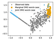
(a) Data for a 1-dimensional regression problem (circle) and the worst case distribution $Q_{0}$ for joint and marginal DRO (triangle/square).

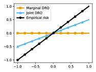
(b) Best fit lines according to each loss. Only marginal DRO selects a line which fits both the $X>0$ and $X<0$ groups.

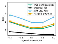
(c) Loss under different regression coefficients. Unlike Marginal DRO, ERM dramatically underestimates and joint DRO overestimates the worst case loss (2).

Figure 1: Toy problem of $L_{1}$ regression through origin.

To illustrate the advantages of the marginal distributionally robust approach, consider a misspecified linear regression problem, where we predict $\widehat{Y}=X\theta$ and use absolute the loss $\ell(\theta;(x,y))=|\theta x-y|$. Letting $\varepsilon\sim\mathsf{N}(0,1)$, the following mixture model generates the data

$$Z\sim\text{Bernoulli}(0.15),~{}~{}~{}X=(1-2Z)\cdot\text{Uniform}([0,1]),~{}~{}~{}Y=|X|+\mathbf{1}\left\{X\geq 0\right\}\cdot\varepsilon$$ (8)

so that the subpopulation $Q_{0}(\cdot):=P(\cdot|Z=1)$ has minority proportion $15\%$. We plot observations from this model in Figure 1(a), where 85% of the points are on the right, and have high noise. The model with the best uniform performance is near $\theta=0$, which incurs similar losses between left and right groups. In contrast, the empirical risk minimizer ($\theta=1$) incurs a high loss of $1$ on the left group and $\sqrt{2/\pi}$ on the right one.

Empirical risk minimization tends to ignore the (left) minority group, resulting in high loss on the minority group $X<0$ (Figure 1(b)). The joint DRO solution (6) minimizes losses over a worst-case distribution $Q_{0}$ consisting of examples that receive high loss (blue triangles), which tend to be samples on $X>0$ due to noise. This results in a loose upper bound on the true worst-case risk as seen in Figure 1(c). Our proposed estimator selects a worst-case distribution consisting of examples with high conditional risk $\mathbb{E}[\ell(\theta;(X,Y))\mid X]$ (Figure 1(a), orange squares). This worst-case distribution is not affected by the noise level, and results in a close approximation to the true loss (Figure 1(c)).

2.2 Estimation via replicates

A natural approach to estimating the dual form (7) is a two phase strategy, where we draw $X_{1},\ldots,X_{n}\stackrel{{\scriptstyle\rm iid}}{{\sim}}P_{X}$ and then—for each $X_{i}$ in the sample—draw a secondary sample of size $m$ i.i.d. from the conditional $Y\mid X=X_{i}$. We then use these empirical samples to estimate $\mathbb{E}[\ell(\theta;(X,Y))\mid X=X_{i}]$. While it is not always possible to collect replicate labels for a single $X$, human annotated data—which is common in machine learning applications [55, 5]—allows replicate measurement, where we may ask multiple annotators to label the same $X$.

We show this procedure can yield explicit finite sample bounds with error at most $O(n^{-1/2}+m^{-1/2})$ for the population marginal robust risk (2) when the losses are bounded.

Assumption A1.

For $M<\infty$, we have $\ell(\theta;(x,y))\in[0,M]$ for all $\theta\in\Theta,x\in\mathcal{X},y\in\mathcal{Y}$.

Since we often want to show uniform concentration guarantees over $\theta\in\Theta$, we make the following standard assumption to control the size of the model class.

Assumption A2.

$\theta\mapsto\ell(\theta;X,Y)$ is $K$-Lipschitz a.s., and $D:=\sup_{\theta,\theta^{\prime}\in\Theta}\left\|{\theta-\theta^{\prime}}\right\|_{2}<\infty$.

The following estimate approximates the worst-case loss (2) for a fixed value of $\theta$.

Proposition 1.

Let Assumption A1 hold. There exists a universal constant $C$ such that for any fixed $\theta\in\Theta$, with probability at least $1-\delta$

$$\Bigg{|}\mathcal{R}(\theta)-\inf_{\eta\in[0,M]}\bigg{\{}\frac{1}{\alpha_{0}n}\sum_{i=1}^{n}\bigg{(}{\frac{1}{m}\sum_{j=1}^{m}\ell(\theta;(X_{i},Y_{i,j}))-\eta}\bigg{)}_{+}+\eta\bigg{\}}\Bigg{|}\leq C\frac{M}{\alpha_{0}}\sqrt{\frac{1+\log\frac{1}{\delta}}{\min\{m,n\}}}.$$

If Assumption A2 also holds, then there exists another universal constant $C^{\prime}$ such that $C^{\prime}\frac{M+DK}{\alpha_{0}}\sqrt{\frac{1+\log\frac{1}{\delta}}{\min\{m,n\}}}$ bounds the left hand side uniformly over $\theta\in\Theta$ with probability at least $1-\delta$.

See Section D.2 for the proof. The estimator in Proposition 1 approximates the worst-case loss (2) well for large enough $m$ and $n$. However—similar to the challenges of making causal inferences from observational data and estimating conditional treatment effects—it is frequently challenging or impossible to collect replicates for individual observations $X$, as each $X$ represents an unrepeatable unique measurement. Consequently, the quantity in Proposition 1 is a type of gold standard, but achieving it can be practically challenging.

3 Variational Approximation to Worst-Case Loss

The difficulty of collecting replicate data, coupled with the conservativeness of the joint DRO objective (6) for approximating the worst-case loss $\mathcal{R}(\theta)$, impel us to study tighter approximations that do not depend on replicates. Recalling the variational representation (3), our goal is to minimize

$$\mathcal{R}(\theta)=\inf_{\eta}\left\{\frac{1}{\alpha_{0}}\sup_{h:\mathcal{X}\to[0,1]}\mathbb{E}_{P}[h(X)(\ell(\theta;(X,Y))-\eta)]+\eta\right\}.$$

As we note in the introduction, this quantity is challenging to work with, so we restrict $h$ to subsets $\mathcal{H}\subset\{h:\mathcal{X}\to[0,1]\}$. The advantage of this formulation and its related relaxations (4) is that it replaces the dependence on the conditional risk with an expectation over the joint distribution on $(X,Y)$, which we may estimate using the empirical distribution, as we describe in the next section.

Each choice of a collection of functions $\mathcal{H}\subset\{h:\mathcal{X}\to[0,1]\}$ to approximate the variational form (3) in the formulation (4) yields a new optimization problem. The lack of a “standard” choice motivates us to perform experiments to direct our development. In Section A, we develop several candidate approximations that are computationally feasible. A priori it is unclear whether different formulations should yield better performance; at least at this point, our theoretical understanding provides similarly limited guidance. To this end, we perform a small simulation study in Section A.2 to direct our coming deeper theoretical and empirical evaluation, discussing the benefits and drawbacks of various choices of $\mathcal{H}$ through the example we introduce in Figure 1(a), Section 2.1. For ease of exposition, we initially defer these comparisons to Section A and focus on developing the approximation method that exhibits the best empirical performance.

We consider the $L^{p}$ upper bound (5) on $\mathcal{R}(\theta)$ as—as we shall see—it provides the best empirical performance. Recall that a function $f:\mathcal{X}\to\mathbb{R}$ is $(\alpha,c)$-Hölder continuous for $\alpha\in(0,1]$ and $c>0$ if $|f(x)-f(x^{\prime})|\leq c\left\|{x-x^{\prime}}\right\|^{\alpha}$ for all $x,x^{\prime}\in\mathcal{X}$. We consider the function class consisting of $L^{p}$ bounded Hölder functions, which we motivate via an $L^{p}$-norm bound (5) on the dual objective (7). For any ${p}\in(1,\infty)$ and $q=\frac{{p}}{{p}-1}$ we have

$$\mathbb{E}_{X\sim P_{X}}\left[\left({\mathbb{E}[\ell(\theta;(X,Y))\mid X]-\eta}\right)_{+}\right]\leq\left(\mathbb{E}_{X\sim P_{X}}\left[\left({\mathbb{E}[\ell(\theta;(X,Y))\mid X]-\eta}\right)_{+}^{p}\right]\right)^{{1/p}}$$

$$\qquad\qquad\qquad~{}=\sup_{h}\left\{\mathbb{E}\left[h(X)(\ell(\theta;(X,Y))-\eta)\right]\mid h:\mathcal{X}\to\mathbb{R}_{+},~{}\mathbb{E}[h(X)^{q}]\leq 1\right\}.$$ (9)

If $x\mapsto\mathbb{E}[\ell(\theta;(X,Y))\mid X=x]$ is Hölder continuous, then the function

$$h^{\star}(x):=\frac{\left({\mathbb{E}[\ell(\theta;(X,Y))\mid X=x]-\eta}\right)_{+}^{{p}-1}}{\left(\mathbb{E}_{X\sim P_{X}}\left[\left({\mathbb{E}[\ell(\theta;(X,Y))\mid X]-\eta}\right)_{+}^{p}\right]\right)^{{1/q}}}$$ (10)

attaining the supremum in the variational form (9) is Hölder continuous with constant dependent on the magnitude of the denominator. As we show shortly, carefully selecting the smoothness constant and $L^{p}$ norm radius allows us to ensure $h^{\star}\in\mathcal{H}$ and to derive guarantees for the resulting estimator.

Minimizing the $L^{p}$ upper bound rather than the original variational objective (alternatively, seeking higher-order robustness than the CVaR of the conditional risk $\mathbb{E}[\ell(\theta;(X,Y))\mid X]$ as in our discussion of the quantity (5)) incurs approximation error. In practice, our experience is that this gap has limited effect, and the following lemma—whose proof we defer to Section D.4—quantifies the approximation error in inequality (9).

Lemma 3.1.

Let Assumption A1 hold and $Z(X)=\mathbb{E}[\ell(\theta;(X,Y))\mid X]$. For $\eta\in[0,M]$

$$\left(\mathbb{E}_{X\sim P_{X}}\left[\left({Z(X)-\eta}\right)_{+}^{p}\right]\right)^{{1/p}}\leq\min\Bigg{\{}(M-\eta)^{{1/q}}\left(\mathbb{E}\left({Z(X)-\eta}\right)_{+}\right)^{{1/p}},$$

$$\qquad\mathbb{E}\left({Z(X)-\eta}\right)_{+}+{p}^{{1/p}}(M-\eta)^{{1/q}}\left(\mathbb{E}\left|\left({Z(X)-\eta}\right)_{+}-\mathbb{E}[\left({Z(X)-\eta}\right)_{+}]\right|\right)^{{1/p}}\Bigg{\}}.$$

We now formally show that the $L^{p}$ variational form provides a tractable upper bound to the worst-case loss for Lipschitzian conditional risks.

Assumption A3.

For $\theta\in\Theta$, the mappings $(x,y)\mapsto\ell(\theta;(x,y))$ and $x\mapsto\mathbb{E}[\ell(\theta;(x,Y))\mid X=x]$ are $L$-Lipschitz.

To ease notation let $\mathcal{H}_{L,{p}}$ denote the space of Hölder continuous functions

$$\mathcal{H}_{L,{p}}:=\left\{h:\mathcal{X}\to\mathbb{R},~{}({p}-1,L^{{p}-1})\mbox{-H\"{o}lder continuous}\right\}.$$ (11)

If Assumption A3 holds and the denominator in the expression (10) has lower bound $\epsilon>0$, then $\epsilon h^{\star}\in\mathcal{H}_{L,{p}}$, and we can approximate the variational form (9) by solving an analogous problem over smooth functions. Otherwise, we can bound the $L^{p}$-norm (9) by $\epsilon^{q-1}$, which is small for small values of $\epsilon$. Hence, if we define a variational objective over smooth functions $\mathcal{H}_{L,{p}}$

$$R_{{p},\epsilon,L}(\theta,\eta):=\sup_{h\in\mathcal{H}_{L,{p}}}\left\{\mathbb{E}\left[\frac{h(X)}{\epsilon}(\ell(\theta;(X,Y))-\eta)\right]~{}~{}\Bigg{|}~{}~{}h\geq 0,~{}\left(\mathbb{E}[h(X)^{q}]\right)^{{1/q}}\leq\epsilon\right\},$$ (12)

we arrive at a tight approximation to the variational form (9), which we prove in Section D.5.

Lemma 3.2.

Let Assumptions A1, A3 hold and let ${p}\in(1,2]$. Then, for any $\theta\in\Theta$ and $\eta\in\mathbb{R}$,

$$\left(\mathbb{E}_{X\sim P_{X}}\left[\left({\mathbb{E}[\ell(\theta;(X,Y))\mid X]-\eta}\right)_{+}^{p}\right]\right)^{{1/p}}=\inf_{\epsilon\geq 0}\left\{R_{{p},\epsilon,L}(\theta,\eta)\vee\epsilon^{q-1}\right\}$$

and for any $\epsilon>0$, $\left(R_{{p},\epsilon,L}(\theta,\eta)\vee\epsilon^{q-1}\right)-\epsilon^{q-1}\leq\left(\mathbb{E}_{X\sim P_{X}}\left[\left({\mathbb{E}[\ell(\theta;(X,Y))\mid X]-\eta}\right)_{+}^{p}\right]\right)^{{1/p}}$.

Empirically, a variational approximation to the $L^{{p}}$-norm bound (5) based on the function class (11) outperforms other potential approximations (Section A.2). We choose to focus on it in the sequel.

4 Tractable Risk Bounds for $L^{p}$ Variational Problem

In this section, we develop an empirical approximation to the $L^{p}$ norm bounded Hölder class, and formally develop and analyze a marginal DRO estimator $\widehat{\theta}^{\rm rob}_{n}$. We derive this estimator by solving an empirical approximation of the upper bound (12) and provide a number of generalization guarantees for this procedure. We complement these results in Section 5 and quantify the fundamental hardness of optimizing over subpopulations $\mathcal{P}_{\alpha_{0},X}$ using finite samples.

4.1 The empirical estimator

Since the variational approximation $R_{{p},\epsilon,L}$ does not use the unknown conditional risk $\mathbb{E}[\ell(\theta;(X,Y))\mid X]$, its empirical plug-in is a natural finite-sample estimator. Defining

$$\widehat{\mathcal{H}}_{L,{p}}:=\left\{h\in\mathbb{R}^{n}:~{}h(X_{i})-h(X_{j})\leq L^{{p}-1}\left\|{X_{i}-X_{j}}\right\|^{{p}-1}~{}~{}\mbox{for all}~{}~{}i,j\in[n]\right\},$$ (13)

we consider the estimator

$$\widehat{R}_{{p},\epsilon,L}(\theta,\eta):=\sup_{h\in\widehat{\mathcal{H}}_{L,{p}}}\left\{\mathbb{E}_{\widehat{P}_{n}}\left[\frac{h(X)}{\epsilon}(\ell(\theta;(X,Y))-\eta)\right]~{}\Bigg{|}~{}h\geq 0,\left(\mathbb{E}_{\widehat{P}_{n}}[h^{q}(X)]\right)^{{1/q}}\leq\epsilon\right\}.$$ (14)

The following lemma shows that the plug-in $\widehat{R}_{{p},\epsilon,L}(\theta,\eta)$ is the infimum of a convex objective.

Lemma 4.1.

For a sample $(X_{1},Y_{1}),\ldots,(X_{n},Y_{n})$ and $B\in\mathbb{R}_{+}^{n\times n}$, define the empirical loss

$$\widehat{R}_{{p},\epsilon,L}(\theta,\eta,B):=\bigg{(}\frac{{p}-1}{n}\sum_{i=1}^{n}\Big{(}{\ell(\theta;(X_{i},Y_{i}))-\frac{1}{n}\sum_{j=1}^{n}(B_{ij}-B_{ji})-\eta}\Big{)}_{+}^{p}\bigg{)}^{{1/p}}+\frac{L^{{p}-1}}{\epsilon n^{2}}\sum_{i,j=1}^{n}\left\|{X_{i}-X_{j}}\right\|^{{p}-1}B_{ij}.$$ (15)

Then $\widehat{R}_{{p},\epsilon,L}(\theta,\eta)=\inf_{B\geq 0}\widehat{R}_{{p},\epsilon,L}(\theta,\eta,B)$ for all $\epsilon>0$.

See Section D.6 for proof. We can interpret dual variables $B_{ij}$ as a transport plan for transferring the loss from example $i$ to $j$ in exchange for a distance dependent cost represented by the last term in the preceding display. The objective $\widehat{R}_{{p},\epsilon,L}(\theta,\eta,B)$ thus consists of transport costs and any losses larger than $\eta$ after smoothing according to the transport plan $B$.

Noting that $\widehat{R}_{{p},\epsilon,L}(\theta,\eta,B)$ is jointly convex in $(\eta,B)$—and jointly convex in $(\theta,\eta,B)$ if the loss $\theta\mapsto\ell(\theta;(X,Y))$ is convex—we consider the empirical minimizer

$$\widehat{\theta}^{\rm rob}_{n,\epsilon}\in\mathop{\rm argmin}_{\theta\in\Theta}\inf_{\eta\in[0,M],B\in\mathbb{R}_{+}^{n\times n}}\left\{\frac{1}{\alpha_{0}}\left(\widehat{R}_{{p},\epsilon,L}(\theta,\eta,B)\vee\epsilon^{q-1}\right)+\eta\right\}$$ (16)

as an approximation to the worst-case mixture covariate shift problem (2). We note that $\widehat{\theta}^{\rm rob}_{n,\epsilon}$ interpolates between the marginal and joint DRO solution; as $L\to\infty$, $B\to 0$ in the infimum over $\widehat{\theta}^{\rm rob}_{n,\epsilon}$ and $\widehat{R}_{{p},\epsilon,L}(\theta,\eta)\to(\frac{p-1}{n}\sum_{i=1}^{n}({\ell(\theta;(X_{i},Y_{i}))-\eta})_{+}^{p})^{1/p}$, an existing empirical approximation to the joint DRO problem [27].

4.2 Generalization and uniform convergence

We now turn to uniform convergence guarantees based on concentration of Wasserstein distances, which show that the empirical minimizer $\widehat{\theta}^{\rm rob}_{n,\epsilon}$ in expression (16) is an approximately optimal solution to the population bound (5). First, we prove that the empirical plug-in (14) converges to its population counterpart at the rate $O(n^{-\frac{p-1}{d+1}})$. For $\alpha\in\left({0},{1}\right]$, define the Wasserstein distance $W_{\alpha}(Q_{1},Q_{2})$ between two probability distributions $Q_{1},Q_{2}$ on a metric space $\mathcal{Z}$ by

$$W_{\alpha}(Q_{1},Q_{2}):=\sup\left\{\left|\mathbb{E}_{Q_{1}}[h]-\mathbb{E}_{Q_{2}}[h]\right|\mid h:\mathcal{Z}\to\mathbb{R},~{}(\alpha,1)\mbox{-H\"{o}lder continuous}\right\}.$$

The following result—whose proof we defer to Section D.7—shows that the empirical plug-in (14) is at most $W_{p-1}(P,\widehat{P}_{n})$-away from its population version.

Lemma 4.2.

Let Assumptions A1, A3 hold, and $\mathop{\rm diam}(\mathcal{X})+\mathop{\rm diam}(\mathcal{Y})\leq R$. For $p\in\left({1},{2}\right],q=p/(p-1)$,

$$\sup_{\theta\in\Theta,\eta\in[0,M]}\left|\epsilon\vee\widehat{R}_{{p},\epsilon,L}(\theta,\eta)-\epsilon\vee R_{{p},\epsilon,L}(\theta,\eta)\right|\leq B_{\epsilon}W_{{p}-1}(\widehat{P}_{n},P)$$

for

$$B_{\epsilon}:=\epsilon^{-q}2^{q-1}RML^{2}+\epsilon^{-1}2^{q-1}L\left(2M+(q-1)LR\right)+\epsilon^{q-2}(q-1)2^{q-2}L+LR.$$ (17)

Our final bound follows from the fact that the Wasserstein distance between empirical and population distributions converges at rate $n^{-(p-1)/(d+1)}$. (See Section D.8 for proof.) In the next subsection, we show that the exponential dependence on the dimension is unavoidable even under more restrictive assumptions on the conditional risk $\mathbb{E}[\ell(\theta;X,Y\mid X]$.

Theorem 1.

Let Assumptions A1, A3 hold, ${p}\in(1,2]$, $\mathop{\rm diam}(\mathcal{X})+\mathop{\rm diam}(\mathcal{Y})\leq R$, and $\frac{d+1}{2}>p-1$. For constants $c_{1},c_{2}>0$ depending on $M,d,{p}$, with probability at least $1-c_{1}\exp\left(-c_{2}n(t^{\frac{d+1}{{p}-1}}\wedge t^{2})\right)$

$$\sup_{Q_{0}(x)\in\mathcal{P}_{\alpha_{0},X}}\mathbb{E}_{X\sim Q_{0}}[ \mathbb{E}[\ell(\widehat{\theta}^{\rm rob}_{n,\epsilon};(X,Y))\mid X]]\leq\inf_{\eta\in[0,M]}\left\{\frac{1}{\alpha_{0}}\left(\mathbb{E}\left[\left({\mathbb{E}[\ell(\widehat{\theta}^{\rm rob}_{n,\epsilon};(X,Y))\mid X]-\eta}\right)_{+}^{p}\right]\right)^{{1/p}}+\eta\right\}$$

$$\leq\inf_{\theta\in\Theta,\eta\in[0,M]}\left\{\frac{1}{\alpha_{0}}\left(\mathbb{E}\left[\left({\mathbb{E}[\ell(\theta;(X,Y))\mid X]-\eta}\right)_{+}^{p}\right]\right)^{{1/p}}+\eta\right\}+\frac{\epsilon^{q-1}}{\alpha_{0}}+\frac{2B_{\epsilon}t}{\alpha_{0}}.$$ (18)

Our concentration bounds exhibit tradeoffs for the worst case loss (2) under mixture covariate shifts; in Theorem 1, the power ${p}$ trades between approximation and estimation error. As ${p}\downarrow 1$, the value $\inf_{\theta\in\Theta}R_{p}(\theta)$ defined by the infimum of the expression (5) over $\theta\in\Theta$ approaches the optimal value $\inf_{\theta\in\Theta}\sup_{Q_{0}\in\mathcal{P}_{\alpha_{0},X}}\underset{X\sim Q_{0}}{\mathbb{E}}[\mathbb{E}[\ell(\theta;(X,Y))\mid X]]$ so that approximation error goes down, but estimation becomes more difficult.

Upper bounds at faster rates

Theorem 1 shows the empirical estimator $\widehat{\theta}^{\rm rob}_{n,\epsilon}$ is approximately optimal with respect to the $L^{{p}}$-bound (5), but with a conservative $O(n^{-\frac{p-1}{d+1}})$-rate of convergence. On the other hand, we can still show that $\widehat{R}_{{p},\epsilon,L}(\theta,\eta)$ provides an upper bound to the worst-case loss under mixture covariate shifts (2) at the faster rate $O(n^{-\frac{1}{4}})$. This provides a conservative estimate on the performance under the worst-case subpopulation. See Section D.9 for the proof.

Proposition 2.

Let Assumptions A1 and A3 hold. There exist numerical constants $c_{1},c_{2}<\infty$ such that the following holds. Let $\theta\in\Theta$, $\epsilon>0$, and ${p}\in\left({1},{2}\right]$. Then with probability at least $1-2\gamma$, uniformly over $\eta\in[0,M]$

$$\mathbb{E}[\left({\mathbb{E}[\ell(\theta;(X,Y))\mid X]-\eta}\right)_{+}^{p}]^{{1/p}}\leq\max\left\{\epsilon^{q-1},(1+\tau_{n})^{q-1}\widehat{R}_{{p},\epsilon,L_{n}(\gamma)}(\theta,\eta)+\frac{c_{1}M^{2}}{\epsilon^{q-1}}\sqrt{\frac{1}{n}\log\frac{1}{\gamma}}\right\}$$

where $\tau_{n}:=c_{2}M^{2}\epsilon^{-q}\sqrt{\frac{1}{n}\log\frac{1}{\gamma}}$ and $L_{n}(\gamma):=L(1+\tau_{n}(\gamma,\epsilon))^{-{1/q}}$. If Assumption A2 further holds, the same bound with $M^{2}+M^{p-1}KD$ in place of $M^{2}$ holds uniformly over $\theta\in\Theta$.

5 Fundamental hardness of marginal DRO

So far in our development, we only required flexible nonparametric assumptions on the conditional risk $\mathbb{E}[\ell(\theta;X,Y)\mid X=x]$ for all $\theta\in\Theta$. We view this as a practically important aspect of our approach; a learning procedure should not depend on unrealistic modeling assumptions. In this section, we show that the pessimistic scaling with the problem dimension we saw in the previous section is unavoidable when considering a nonparametric class of conditional risks. Optimization of both the original worst-case subpopulation risk (2) and the $L^{p}$-norm the upper bound are governed by similar pessimistic dependence on the dimension.

We study the fundamental hardness of optimizing the worst-case subpopulation risk $\mathcal{R}(\theta;P)=\sup_{Q_{0}\in\mathcal{P}_{\alpha_{0},X}(P)}\underset{X\sim Q_{0}}{\mathbb{E}}[\mathbb{E}_{P}[\ell(\theta;X,Y)\mid X]]$, where we now make explicit the dependence on the data-generating distribution $P$ in the notation. We show that the fundamental statistical difficulty of solving marginal DRO problems follow a standard nonparametric rate when only requiring the conditional risk $x\mapsto\mathbb{E}_{P}[\ell(\theta;X,Y)\mid X=x]$ to be a Hölder-smooth function. Recall that the Hölder class $\Lambda^{\beta}$ of $\beta$-smooth functions for $\beta_{1}=\left\lceil{\beta}\right\rceil-1$ and $\beta_{2}=\beta-\beta_{1}$ is

$$\Lambda^{\beta}:=\left\{\mu(\cdot)\in C^{\beta_{1}}(\mathcal{X}):\sup_{\tiny\begin{array}[]{c}x\in\mathcal{X}\\ \sum_{k=1}^{d}\gamma^{k}<\beta_{1}\end{array}}|D^{\gamma}\mu(x)|\leq 1,~{}\sup_{\tiny\begin{array}[]{c}x\neq x^{\prime}\in\mathcal{X}\\ \sum_{k=1}^{d}\gamma^{k}=\beta_{1}\end{array}}\frac{|D^{\gamma}\mu(x)-D^{\gamma}\mu(x^{\prime})|}{\left\|{x-x^{\prime}}\right\|^{\beta_{2}}}\leq 1\right\},$$ (19)

where $C^{\beta_{1}}(\mathcal{X})$ denotes the space of $\beta_{1}$-times continuously differentiable functions on $\mathcal{X}$, and $D^{\gamma}=\frac{\partial^{\gamma}}{\partial^{\gamma^{1}}\ldots\partial^{\gamma^{d}}}$, for any $d$-tuple of nonnegative integers $\gamma=(\gamma^{1},\ldots,\gamma^{d})$. Let $\mathfrak{P}_{\beta}$ be the set of data-generating distributions with Hölder smooth conditional risk uniformly over $\theta\in\Theta$

$$\mathfrak{P}_{\beta}:=\left\{P:\mathbb{E}_{P}[\ell(\theta;X,Y)\mid X=\cdot]\in\Lambda^{\beta}~{}~{}\mbox{for~{}all}~{}\theta\in\Theta,~{}|Y|\leq 1~{}P\mbox{-a.s.}\right\}.$$

We study the finite sample minimax risk for a sample of size $n$

$$\mathcal{M}_{n}:=\inf_{\widehat{\theta}}\sup_{P\in\mathfrak{P}_{\beta}}\mathbb{E}_{P}\left[\mathcal{R}(\widehat{\theta};P)-\inf_{\theta\in\Theta}\mathcal{R}(\theta;P)\right]$$ (20)

where the outer infimum is over all measurable functions of the data $\{X_{i},Y_{i}\}_{i=1}^{n}$. In the definition (20), the inner supremum is not to be confused with the worst-case over subpopulations in $\mathcal{P}_{\alpha_{0},X}$ defining our distributionally robust formulation. With this, in Appendix D.10 we prove the following.

Theorem 2.

Let $\mathcal{X}=[0,1]^{d}$, $\Theta=[0,1]$, $\ell(\theta;X,Y)=\theta\cdot Y$. There are constants $N,c>0$ depending on $(d,\alpha_{0},\beta)$, such that for all $n\geq N$, $\mathcal{M}_{n}\geq cn^{-\frac{2\beta}{2\beta+d^{\prime}}}$ where $d^{\prime}=d$ for odd $d$ and $d-1$ for even $d$.

Our minimax lower bound shows that the exponential sample complexity in the dimension $d$ is unavoidable in the nonparametric minimax sense (20), so that while the bounds Theorem 1 guarantees may not be completely sharp, the worst-case exponential dependence on dimension $d$ is real. As is typical in nonparametric estimation, we recover parametric rates as $\beta\to\infty$. More carefully identifying the (problem-dependent) constants $c,N$ remains a goal of future work.

A similar argument shows it is equally difficult to optimize the $L_{p}$-upper bound (5) on the worst-case subpopulation risk. We again study the finite sample minimax risk for a sample of size $n$

$$\mathcal{M}_{n,p}:=\inf_{\widehat{\theta}}\sup_{P\in\mathfrak{P}_{\beta}}\mathbb{E}_{P}\left[\mathcal{R}_{{p}}(\widehat{\theta};P)-\inf_{\theta\in\Theta}\mathcal{R}_{{p}}(\theta;P)\right]$$

where the outer infimum is over all measurable functions of the data $\{X_{i},Y_{i}\}_{i=1}^{n}$. In Appendix D.11, we prove the following result via a trivial adaptation of the proof of Theorem 2.

Corollary 1.

Let the conditions of Theorem 2 hold. There are constants $N,c>0$ depending on $(d,\alpha_{0},\beta)$ such that for $n\geq N$, $\mathcal{M}_{n,p}\geq cn^{-\frac{2\beta}{2\beta+d^{\prime}}}$ where $d^{\prime}=d$ for odd $d$ and $d-1$ for even $d$.

6 Experiments

We now present empirical investigations of the procedure (16), focusing on two main aspects of our results. First, our theoretical results exhibit nonparametric rates of convergence, so it is important to understand whether these upper bounds on convergence rates govern empirical performance and the extent to which the procedure is effective. Second, on examples with high conditional risk $\mathbb{E}[\ell(\theta;(X,Y))\mid X]$, we expect our procedure to improve performance on minority groups and hard subpopulations when compared against joint DRO and empirical risk minimization (ERM). The code for all experiments can be found in https://github.com/hsnamkoong/marginal-dro.

To investigate both of these issues, we begin by studying simulated data (Section 6.1) so that we can evaluate true convergence precisely. We see that in moderately high dimensions, our procedure outperforms both ERM and joint DRO on worst-off subpopulations; we perform a parallel simulation study in Section B.1 for the confounded case (minimizing $\widehat{R}_{{p},\epsilon,L,\delta}(\theta,\eta)$ of Lemma B.2). After our simulation study, we continue to assess the efficacy of our procedure on real data, using our method to predict semantic similarity (Section 6.2), wine quality (Section 6.3) and crime recidivism (Section 6.4). In all of these experiments, our results are consistent with our expectation that our procedure (16) typically improves performance over unseen subpopulations.

Hyperparameter choice is important in our procedures. We must choose a Lipschitz constant $L$, worst-case group size $\alpha_{0}$, risk level $\epsilon$, and moment parameter ${p}$. In our experiments, we see that cross-validation is attractive and effective. We treat the value $L/\epsilon$ as a single hyperparameter to estimate via a hold-out set or, in effort to demonstrate sensitivity to the parameter, plot results across a range of $L/\epsilon$. As the objective (16) is convex standard methods apply; we use (sub)gradient descent to optimize the problem parameters over $\theta,\eta,B$. In each experiment, we compare our marginal DRO method against two baselines: empirical risk minimization (ERM) and joint DRO (6). ERM minimizes the empirical risk $\mathop{\rm minimize}_{\theta\in\Theta}\mathbb{E}_{\widehat{P}_{n}}[\ell(\theta;(X,Y))]$, and provides very weak guarantees on subpopulation performance. The joint DRO formulation (6) is the only existing method that provides an upper bound to the worst-case risk. We evaluate empirical plug-ins of the dual formulation ($p\geq 1$)

$$\inf_{\eta\in\mathbb{R}}\left\{\frac{1}{\alpha_{0}}\mathbb{E}[\left({\ell(\theta;(X,Y))-\eta}\right)_{+}^{p}]^{1/p}+\eta\right\},$$ (21)

which is the joint DRO counterpart of our marginal DRO procedure (16) for the same value of $p$. Joint DRO formulations over other uncertainty sets (e.g. Wasserstein balls [47]) do not provide guarantees on subpopulation performance as they protect against different distributional shifts, including adversarial attacks [72].

6.1 Simulation study: the unconfounded case

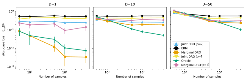
Figure 2: Dimension and sample size dependence of robust loss surrogates. The two marginal DRO methods correspond to different choices in the variational approximation ($L_{p}$ Hölder and Bounded Hölder).

Our first simulation study focuses on the unconfounded procedure (16), where the data follows the distribution (28), and the known ground truth allows us to carefully measure the effects of the problem parameters $(n,d,\alpha)$ and sensitivity to the smoothness assumption $L$. We focus on the regression example from Sec. A.2 with loss $\ell(\theta;x,y)=|\theta^{\top}x-y|$, so the procedure (16) is an empirical approximation to minimizing the worst-case objective $\sup_{Q_{0}\in\mathcal{P}_{\alpha_{0},X}}\underset{X\sim Q_{0}}{\mathbb{E}}\left[\mathbb{E}[|\theta^{\top}X-Y|\mid X]\right]$.

The simulation distribution (28) captures several aspects of loss minimization in the presence of heterogeneous subpopulations. The subpopulations $X_{1}\geq 0$ and $X_{1}<0$ constitute a majority and minority group, and minimizing the risk of the majority group comes at the expense of risk for the minority group. The two subpopulations also define an oracle model that minimizes the maximum loss over the two groups. As the uniform distribution exhibits the slowest convergence of empirical distributions for Wasserstein distance [31]—and as Wasserstein convergence underpins our $n^{-1/d}$ rates in Lemma 4.2—we use the uniform distribution over covariates $X$. We train all DRO models with worst-case group size $\alpha_{0}=0.3$ and choose the estimated Lipschitz parameter $L/\epsilon$ by cross-validation on a replicate-based estimate of the worst-case loss (22) (below) using a held-out set of 1000 examples and 100 repeated measurements of $Y$. We do not regularize as $d\ll n$.

Effect of the $p$-norm bound

We evaluate the difference in model quality as a function of $p$, which controls the tightness of the $p$-norm upper bound. Our convergence guarantees in Theorem 1 are looser for $p$ near $1$, though such values achieve smaller asymptotic bias to the true sub-population risk, while values of $p$ near 2 suggest a more favorable sample size dependence in the theorem.

In Figure 2, we plot the results of experiments for each suggested procedure, where the horizontal axes index sample size and the vertical axes an empirical approximation to the worst-case loss

$$R_{\alpha_{0}}(\theta):=\sup_{Q_{0}\in\mathcal{P}_{\alpha_{0},X}}\underset{X\sim Q_{0}}{\mathbb{E}}\mathbb{E}\left[|\theta^{\top}X-Y|\mid X\right]$$ (22)

over the worst 5% of the population (test-time $\alpha_{0}=0.05$); the plots index dimensions $d=1,10,50$. . We evaluate a worst-case error smaller than the true mixture proportion to measure our procedure’s robustness within the minority subgroup. The plots suggest that the choice $p=2$ (Marginal DRO) outperforms $p=1$ (Linf Marginal DRO), and performance generally seems to degrade as $p\downarrow 1$. We consequently focus on the $p=2$ case for the remainder of this section.

Sample size and dimension dependence

We use the same experiment to also examine the pessimistic $O(n^{-1/d})$ convergence rate of our estimator (16); this is substantially worse than that for ERM and joint DRO (6), both of which have convergence rates scaling at worst as $1/\sqrt{n}$ [27]. In low dimensions ($d=1$ to $d=10$) convergence to the optimal function value—which we can compute exactly—is relatively fast, and marginal DRO becomes substantially better with as few as 500 samples (Figure 2). In higher dimensions ($d=50$), marginal DRO convergence is slower, but it is only worse than the joint DRO solution when $n=d=100$. At large sample sizes $n>1000$, marginal DRO begins to strictly outperform the two baselines as measured by the worst-case 5% loss (22).

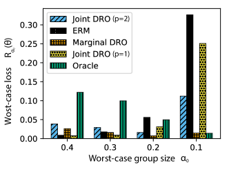
(a) Loss for various worst group sizes.

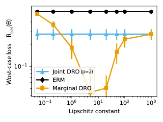
(b) Marginal DRO losses across $L/\epsilon$

Figure 3: Sensitivity of marginal DRO losses to test-time worst-case group size (left) and Lipschitz constant estimate (right).

Additional extended results in the supplement demonstrate that these results are robust to changes in the type of loss ($L_{1}$ vs $L_{2}$) Section C.2 and can be obtained with only a factor of 2 computational overhead Section C.1.

Sensitivity to robustness level

We rarely know the precise minority proportion $\alpha_{\rm true}$, so that in practice one usually provides a postulated lower bound $\alpha_{0}$; we investigate sensitivity to its specification. We fix the data generating distribution $\alpha_{\rm true}=0.15$ and train DRO models with $\alpha_{0}=0.3$, while evaluating them using varying test-time worst case group size $\alpha_{0}$ in Eq. 22. We show the results of varying the test-time worst-case group size in Figure 3(a). Marginal DRO obtains a loss within $1.2$ times the oracle model regardless of the test-time worst-case group size, while both ERM and joint DRO incur substantially higher losses on the tails.

Sensitivity to Lipschitz constant

Finally, the empirical bound (18) requires an estimate of the Lipschitz constant of the conditional risk. We vary the estimate $L/\epsilon$ in Figure 3) for $\alpha=0.3$, $d=2$, and $n=1000$, showing that the marginal robustness formulation has some sensitivity to the parameter, though there is a range of several orders of magnitude through which it outperforms the joint DRO procedures. The behavior that it exhibits is expected, however: the choice $L=0$ reduces the marginal DRO procedure to ERM in the bound (18), while the choice $L=\infty$ results in the joint DRO approach. In higher dimensions, marginal DRO will increasingly behave like joint DRO, leading to a smaller range of Lipschitz constants where marginal DRO performs well.

6.2 Semantic similarity prediction

We now present the first of our real-world evaluations of the marginal DRO procedure (16), focusing on a setting where we have multiple measured outcome labels $Y$ for each covariate $X$, so it is possible to accurately estimate the worst-case loss over covariate shifts. We consider the WS353 lexical semantic similarity prediction dataset [2] where the features are pairs of words, and labels are a set of $13$ human annotations rating the word similarity on a $0$–$10$ scale. In this task, our goal is to use noisy human annotations of word similarities to learn a robust model that accurately predicts word similarities over a large set of word pairs.

We represent each word pair as the difference $(x_{1}-x_{2})$ of the word vectors $x_{1}$ and $x_{2}$ associated to each word in GloVe [60] and cast this as a standard metric learning task of predicting a scalar similarity $Y$ with a word-pair vector $X$ via the quadratic model $x\mapsto x^{\top}\theta_{1}x+\theta_{2}$, $\theta_{1}\in\mathbb{R}^{d\times d}$, $\theta_{2}\in\mathbb{R}$. We use the absolute deviation loss $|y-x^{\top}\theta_{1}x+\theta_{2}|$. The training set consists of $1989$ individual annotations of word similarities (ignoring any replicate structure), and we fit the marginal DRO model with $p=2$, joint DRO models (21) with $p=1,2$, and an ERM model. All methods use the same ridge regularizer tuned for the ERM model. We train all DRO procedures using $\alpha_{0}=0.3$ and tune the Lipschitz constant via a held out set using the empirical estimate to the worst-case loss based on replicate annotations (as in Proposition 1).

To evaluate each model $\theta=(\theta_{1},\theta_{2})$, we take an empirical approximation to the worst-case loss over the word pairs with respect to the averaged human annotation

$$R_{\alpha_{0}}(\theta):=\sup_{Q_{0}\in\mathcal{P}_{\alpha_{0},X}}\underset{X\sim Q_{0}}{\mathbb{E}}\left[|X^{\top}\theta_{1}X+\theta_{2}-\mathbb{E}\left[Y\mid X\right]|\right].$$ (23)

This is a worst-case version of the standard word similarity evaluation [60], where we also use averaged replicate human annotations as the ground truth $\mathbb{E}[Y\mid X]$ in our evaluations, and consider test-time worst-case group sizes $\alpha_{0}$ ranging from 0.01 to 1.0.

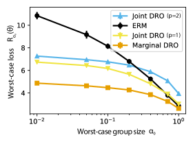
Figure 4: Semantic similarity prediction task, with worst-case prediction error $R_{\alpha_{0}}(\theta)$ (Eq. 23) over subgroups (y-axis) evaluated over varying test time worst-case group sizes $\alpha_{0}$ (x-axis).

All methods achieve low average error over the entire dataset, but ERM, joint DRO and marginal DRO exhibit disparate behaviors for small subgroups. ERM incurs large errors at $\sim 5\%$ of the test set, resulting in near random prediction. Applying the joint DRO estimator reduces error by nearly half and marginal DRO reduces this even further (Figure 4).

6.3 Distribution shifts in wine quality prediction

Next, we show that marginal DRO ($p=2$) can yield improvements outside of the worst-case subgroup assumptions we have studied thus far. The UCI wine dataset [24] is a regression task with 4898 examples and 12 features, where each example is a wine with measured chemical properties and the label $y\in\mathbb{R}$ is a subjective quality assessment; the data naturally splits into subgroups of white and red wines. We consider a distribution shift problem where the regression model is trained on red wines but tested on (subsets of) white wines. Unlike the earlier examples, the test set here does not correspond to subpopulations of the training distribution, and the chemical features of red wine are likely distinct from those for white wines, violating naive covariate shift assumptions.

We minimize the absolute deviation loss $\ell(\theta;x,y)=|\theta^{\top}x-y|$ for linear predictions, tuning baseline parameters (e.g. ridge regularization) on a held-out set that is i.i.d. with the training distribution. Our training distribution is 1500 samples of red wines and the test distribution is all white wines. We evaluate models via their loss over worst-case subgroups of the white wines, though in distinction from earlier experiments, we have no replicate labels. Thus we measure the joint DRO loss (6), i.e.

$$R_{\alpha_{0},\mbox{\scriptsize joint}}(\theta):=\sup_{Q_{0}\in\mathcal{P}_{\alpha_{0},(X_{w},Y_{w})}}\underset{X_{w},Y_{w}\sim Q_{0}}{\mathbb{E}}\left[|\theta^{\top}X_{w}-Y_{w}|\right],$$

so that the worst-case loss $R_{\alpha_{0},\mbox{\scriptsize joint}}(\theta)$ measures the subgroup losses under the white wine distribution.

Figure 8 shows the worst-case loss $R_{\alpha_{0},\mbox{\scriptsize joint}}(\theta)$ over the test set as a function of $\alpha_{0}$. Here, Marginal DRO with Lipschitz constants $L/\epsilon$ varying over $0.1$ to $300$ and $\alpha_{0}=0.3$ provides improvements over both joint DRO and ERM baselines across the entire range of test-time $\alpha_{0}$. Marginal DRO improves losses both for the pure distribution shift from red to white wines (test-time group size $\alpha=1.0$) as well as for the more pessimistic groups with small test-time proportion $\alpha_{0}$. Distribution shift from red to white wines appears difficult to capture for the pessimistic joint DRO methods.

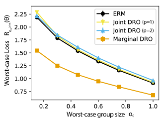
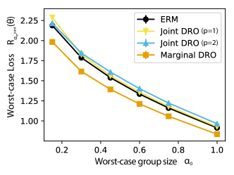
Figure 5: Marginal DRO improves worst-case loss $R_{\alpha_{0},\mbox{\scriptsize joint}}(\theta)$ for the wine quality prediction task under a real world red to white wine distribution shift. The gain holds on a wide range of Lipschitz constants from $L/\epsilon=0.1$ (left) to $300$ (right).

6.4 Recidivism prediction

Finally, we show that marginal DRO $(p=2)$ can control the loss over a minority group on a recidivism prediction task. The COMPAS recidivism dataset [23] is a classification task where examples are individual convicts, features consist of binary demographic labels (such as African American or not) and description of their crimes, and the label is whether they commit another crime after release (recidivism). We use the fairML toolkit version of this dataset [1]. Classification algorithms for recidivism have systematically discriminated against minority groups, and this dataset illustrates such discrimination [6]. We consider this dataset from the perspective of achieving uniform performance across various groups. There are $10$ binary variables in data, each indicating a potential split of the data into minority and majority group (e.g. young vs. not young, or Black vs. non-Black), of which $7$ have enough ($n>10$) observations in each split to make reasonable error estimates. We train a model over the full population (using all the features), and for each of the $7$ demographic indicator variables and evaluate the held-out 0-1 loss over both the associated majority group and minority group.

Our goal is to ensure that the classification accuracy remains high without explicitly splitting the data on particular demographic labels (though we include them in our models as they have predictive power). We use the binary logistic loss with linear models and a $70/30$ train/test split. We set $\alpha_{0}=0.4$ for all DRO methods (approximately matching demographic statistics in the United States, with 60% white and 40% other races), and apply ridge regularization to all models with regularization parameter tuned for the ERM model.

Method	Old	Young	Black	Hispanic	Other race	Female	Misdemeanor
ERM	37.7 $\pm$ 0.8	44.6 $\pm$ 1.0	37.7 $\pm$ 0.8	37.5 $\pm$ 0.9	37.9 $\pm$ 1.1	37.5 $\pm$ 0.9	37.6 $\pm$ 0.8
Joint ($p=2$) - ERM	10.0 $\pm$ 2.0	4.0 $\pm$ 1.7	9.7 $\pm$ 1.7	9.6 $\pm$ 1.8	10.9 $\pm$ 2.3	9.2 $\pm$ 1.8	9.0 $\pm$ 1.6
Joint ($p=1$) - ERM	5.8 $\pm$ 1.7	1.2 $\pm$ 1.7	5.2 $\pm$ 1.5	7.4 $\pm$ 1.9	6.6 $\pm$ 2.1	5.9 $\pm$ 1.7	5.1 $\pm$ 1.5
Marginal L=0.01 - ERM	-0.7 $\pm$ 0.7	1.4 $\pm$ 1.1	-1.0 $\pm$ 0.7	-1.7 $\pm$ 0.9	-2.4 $\pm$ 1.1	-1.5 $\pm$ 0.8	-1.5 $\pm$ 0.7
Marginal L=0.001 - ERM	-1.1 $\pm$ 0.7	0.4 $\pm$ 1.1	-1.4 $\pm$ 0.7	-2.1 $\pm$ 0.9	-2.6 $\pm$ 1.1	-1.9 $\pm$ 0.8	-1.8 $\pm$ 0.7

Table 1: Worst-case error of recidivism prediction models across demographic subgroups. The ERM row shows baseline worst-case error; subsequent rows show error differences from baseline (negatives indicate lower error).

Table 6.4 presents the 0-1 loss on the seven demographic splits over 100 random train/test splits. For each attribute (table column) we split the test set into examples for which the attribute is true and false and report the average 0-1 loss on the worst of the two groups. The first row gives the average worst-case error and associated 95% standard error for the ERM model. For the DRO based models (remaining rows), we report the average differences with respect to the baseline ERM model and standard error intervals. Unlike our earlier regression tasks, joint DRO (both $L_{2}$ and $L_{1}$) performs worse than ERM on almost all demographic splits. On the other hand, we find that marginal DRO with the appropriate smoothness constant $L\in\{10^{-2},10^{-3}\}$ reduces classification errors between $1$–$2\%$ on the worst-case group across various demographics, with the largest error reduction of 3% occurring in the young vs. old demographic split.

Appendix A Alternative variational approximations

Recalling the variational representation (3), we wish to minimize the variational approximation

$$\inf_{\eta}\left\{\frac{1}{\alpha_{0}}\sup_{h\in\mathcal{H}}\mathbb{E}_{P}[h(X)(\ell(\theta;(X,Y))-\eta)]+\eta\right\}.$$

For each choice of $\mathcal{H}$ we propose below, we consider an empirical approximation $\widehat{\mathcal{H}}$, the subset of $\mathcal{H}$ restricted to mapping $\{X_{1},\ldots,X_{n}\}\to\mathbb{R}$ instead of $\mathcal{X}\to\mathbb{R}$, solving the empirical alternative

$$\mathop{\rm minimize}_{\theta\in\Theta,\eta}\left\{\frac{1}{\alpha_{0}}\sup_{h\in\widehat{\mathcal{H}}}\mathbb{E}_{\widehat{P}_{n}}[h(X)(\ell(\theta;(X,Y))-\eta)]+\eta\right\}.$$ (24)

We design our proposals so the dual of the inner supremum (24) is computable. When the conditional risk $x\mapsto\mathbb{E}[\ell(\theta;(X,Y))\mid X=x]$ is smooth, we can provide generalization bounds for our procedures. We omit detailed development for our first two procedures—which we believe are natural proposals, justifying a bit of discussion—as neither is as effective as the last procedure in our empirical evaluations, which controls the $L^{p}$ upper bound (5) on $\mathcal{R}(\theta)$.

A.1 Example approximations and empirical variants

Reproducing Hilbert kernel spaces (RKHS)

Let $K:\mathcal{X}\times\mathcal{X}\to\mathbb{R}_{+}$ be a reproducing kernel [11, 4] generating the reproducing kernel Hilbert space $\mathcal{H}_{K}$ with associated norm $\left\|{\cdot}\right\|_{K}$. For any $R\in\mathbb{R}_{+}$, we can define a norm ball

$$\mathcal{H}_{K,R}:=\left\{h\in\mathcal{H}_{K}:\left\|{h}\right\|_{K}\leq R,h\in[0,1]\right\}$$

and consider the variational approximation (4) with $\mathcal{H}=\mathcal{H}_{K,R}$. To approximate the population variational problem $\sup_{h\in\mathcal{H}_{K,R}}\mathbb{E}[h(X)(\ell(\theta;(X,Y))-\eta)]$, we consider a restriction of the same kernel $K$ to the sample space $\{X_{1},\ldots,X_{n}\}$. Let $K_{n}=\{K(X_{i},X_{j})\}_{1\leq i,j\leq n}$ be the Gram matrix evaluated on samples $X_{1},\ldots,X_{n}$, and define the empirical approximation

$$\widehat{\mathcal{H}}_{K,R}:=\left\{h\in[0,1]^{n}:h=K_{n}\xi~{}\mbox{ for some}~{}\xi\in\mathbb{R}^{n}~{}\mbox{such that}~{}\frac{1}{n^{2}}\xi^{\top}K_{n}\xi\leq R\right\}.$$

(Recall that if $h(x)=\sum_{i=1}^{n}K(x,X_{i})\xi_{i}$, then $\left\|{h}\right\|_{K}^{2}=\frac{1}{n^{2}}\xi^{\top}K_{n}\xi$.) To compute the empirical problem (24) with $\widehat{\mathcal{H}}=\widehat{\mathcal{H}}_{k,R}$, we take the dual of the inner supremum. Simplifying the dual form—whose derivation is a standard exercise in convex optimization—we get

$$\mathop{\rm minimize}_{\theta\in\Theta,\eta\in\mathbb{R},\beta\in\mathbb{R}^{n}}\left\{\frac{1}{\alpha_{0}n}\sum_{i=1}^{n}\left({\ell(\theta;(X_{i},Y_{i}))-\eta+\beta_{i}}\right)_{+}+\frac{1}{n}\sqrt{R^{-1}\beta^{\top}K_{n}\beta}\right\}.$$ (25)

For convex losses $\ell(\theta;(X,Y))$, this is a convex optimization problem in $(\theta,\beta,\eta)$.

Hölder continuous functions (bounded Hölder)

Instead of the space of bounded functions, we restrict attention to Hölder continuous functions

$$\mathcal{H}_{L,{p}}:=\left\{h:\mathcal{X}\to[0,1]\mid h~{}\mbox{is}~{}~{}({p}-1,L^{{p}-1})\mbox{-H\"{o}lder continuous}\right\},$$ (26)

where the particular scaling with respect to ${p}\in(1,2]$ and $L>0$ is for notational convenience in Section 4. The empirical plug-in of $\mathcal{H}_{L,{p}}$ is

$$\widehat{\mathcal{H}}_{L,p}:=\left\{h:\{X_{1},\ldots,X_{n}\}\to[0,1]\mid h~{}\mbox{is}~{}({p}-1,L^{{p}-1})\mbox{-H\"{o}lder continuous}\right\},$$

the empirical plug-in of the variational problem (4) with $\mathcal{H}=\mathcal{H}_{L,{p}}$ is given by the procedure (24) with $\widehat{\mathcal{H}}=\widehat{\mathcal{H}}_{L,p}$. Taking the dual of the inner supremum problem, we have the following equivalent dual formulation of the empirical variational problem

$$\mathop{\rm minimize}_{\theta\in\Theta,\eta,B\in\mathbb{R}^{n\times n}_{+}}\bigg{\{}\frac{1}{\alpha_{0}n}\sum_{i=1}^{n}\Big{(}{\ell(\theta;(X_{i},Y_{i}))-\frac{1}{n}\sum_{j=1}^{n}(B_{ij}-B_{ji})-\eta}\Big{)}_{+}+\frac{L^{{p}-1}}{n^{2}}\sum_{i,j=1}^{n}\left\|{X_{i}-X_{j}}\right\|^{{p}-1}B_{ij}\bigg{\}}.$$ (27)

For convex losses $\theta\mapsto\ell(\theta;(X,Y))$, this is again a convex optimization problem in $(\theta,B,\eta)$, and is always smaller than the empirical joint DRO formulation (6).

By definition, the population Hölder continuous variational approximation provides the lower bound on the worst-case loss

$$\mathcal{R}_{L,{p}}(\theta):=\inf_{\eta}\sup_{h\in\mathcal{H}_{L,{p}}}\left\{\frac{1}{\alpha_{0}}\mathbb{E}_{P}[h(X)(\ell(\theta;(X,Y))-\eta)]+\eta\right\}\leq\mathcal{R}(\theta).$$

As a consequence, $\mathcal{R}_{L,{p}}$ cannot upper bound the subpopulation loss $\mathbb{E}_{X\sim Q_{0}}[\mathbb{E}[\ell(\theta;(X,Y))\mid X]]$ uniformly over $Q_{0}\in\mathcal{P}_{\alpha_{0},X}$. Nonetheless, for any subpopulation $Q_{0}\in\mathcal{P}_{\alpha_{0},X}$ with Lipschitz density $\frac{dQ_{0}}{dP}:\mathcal{X}\to\mathbb{R}_{+}$, then $\mathcal{R}_{L,2}(\theta)$ does provide a valid upper bound on $\mathbb{E}_{X\sim Q_{0}}[\mathbb{E}[\ell(\theta;(X,Y))\mid X]]$:

Lemma A.1.

Let $Q_{0}\in\mathcal{P}_{\alpha_{0},X}$ be any distribution with $L$-Lipschitz density $\frac{dQ_{0}}{dP}:\mathcal{X}\to\mathbb{R}_{+}$. Then

$$\mathbb{E}_{X\sim Q_{0}}[\mathbb{E}[\ell(\theta;(X,Y))\mid X]]\leq\mathcal{R}_{L,2}(\theta)\leq\mathcal{R}(\theta).$$

See Section D.3 for a proof. For example, if $P$ and $Q_{0}\in\mathcal{P}_{\alpha_{0},X}$ both have Lipschitz log densities, then $\frac{dQ_{0}}{dP}$ is also Lipschitz, as the following example shows.

Example 1:  Let $P$ be absolutely continuous with respect to some $\sigma$-finite measure $\mu$, denote $p(X):=\frac{dP}{d\mu}(X)$ and $q_{0}(X):=\frac{dQ_{0}}{d\mu}(X)$ and assume $\log p$ and $\log q_{0}$ are $L$-Lipschitz. Let $h(x):=\frac{q_{0}(x)}{p(x)}$, and consider any fixed $x,x^{\prime}\in\mathcal{X}$. If we assume that without loss of generality that $h(x)$ > $h(x^{\prime})$, then

$$\frac{\left|h(x)-h(x^{\prime})\right|}{\|x-x^{\prime}\|} =\frac{h(x)}{\left\|{x-x^{\prime}}\right\|}\left(1-\exp\Big{(}\log\frac{p(x)}{q_{0}(x)}-\log\frac{p(x^{\prime})}{q_{0}(x^{\prime})}\Big{)}\right)\leq\frac{L}{\alpha_{0}},$$

where the final inequality follows because $h(x)=q_{0}(x)/p(x)\leq 1/\alpha_{0}$ and $\exp(x)\geq 1+x$. Consequently, then $x\mapsto q_{0}(x)/p(x)$ is $(L/\alpha_{0})$-Lipschitz. $\Diamond$

A.2 Empirical Comparison of Variational Procedures

We consider an elaborated version of the data mechanism (8) to incorporate higher dimensionality, with the data generating distribution

$$\begin{split}Z\sim\mathsf{Bern}(0.15),~{}~{}&X_{1}=(1-2Z)\cdot\mathsf{Uni}([0,1]),~{}~{}X_{2},\ldots,X_{d}\stackrel{{\scriptstyle\rm iid}}{{\sim}}\mathsf{Uni}([-1,1])\\ &Y=|X_{1}|+\mathbf{1}\left\{X_{1}\geq 0\right\}\cdot\varepsilon,~{}~{}~{}\varepsilon\sim\mathsf{N}(0,1).\end{split}$$ (28)

Our goal is to predict $Y$ via $\widehat{Y}=\theta^{\top}X$, and we use the absolute loss $\ell(\theta;(x,y))=|y-\theta^{\top}x|$. We provide details of the experimental setup, such as the estimators and optimizers, in Section 6. In brief, we perform a grid search over all hyperparameters (Lipschitz estimates and kernel scales) for each method over 4 orders of magnitude; for the RKHS-based estimators, we test Gaussian, Laplacian, and Matern kernels, none of which have qualitative differences from one another, so we present results only for the Gaussian kernel $K(x,x^{\prime})=\exp(-\frac{1}{2\sigma^{2}}\left\|{x-x^{\prime}}\right\|_{2}^{2})$.

Dimension dependence

We first investigate the dimension dependence of the estimators, increasing $d$ in the model (28) from $d=2$ to $50$ with a fixed sample size $N=5000$.

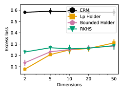
Figure 6: Variational estimates based on RKHS are less affected by the dimensionality of the problems, but perform worse than the Hölder continuous function approaches overall.

Under model (28), we consider marginal distributionally robust objective (2) and evaluate the excess risk $\mathcal{R}(\theta)-\inf_{\theta}\mathcal{R}(\theta)$ for the choice $\alpha_{0}=.15$, the hardest 15% of the data. As $d$ grows, we expect estimation over Hölder continuous functions to become more difficult, and for the RKHS-based estimator to outperform the others. Figure 6 bears out this intuition (plotting the excess risk): high dimensionality induces less degradation in the RKHS approach than the others. Yet the absolute performance of the Hölder-based methods is better, which is unsurprising, as we are approximating a discontinuous indicator function.

Sample size dependence

We also consider the sample dependence of the estimators, fitting models using losses with robustness level set to $\alpha_{0}=.15$, then evaluating their excess risk $\mathcal{R}(\widehat{\theta})-\inf_{\theta}\mathcal{R}(\theta)$ using $\alpha_{0}\in\{.05,.15\}$, so that we can see the effects of misspecification, as it is unlikely in practice that we know the precise minority population size against which to evaluate. Unlike the $L^{p}$-Hölder class (Eq. (9)), the bounded $c$-Hölder continuous function class (26) can approximate the population optimum of the original variational problem (3) as $n\to\infty$ and $c\to\infty$. Because of this, we expect that as the sample size grows, and $c$ is set optimally, the bounded Hölder class will perform well.

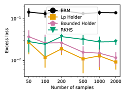
(a) $\alpha_{0}=0.15$ for both train and test.

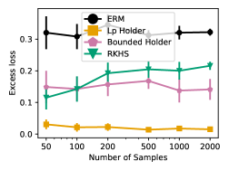
(b) $\alpha_{0}=0.15$ for training, $\alpha_{0}=0.05$ for testing.

Figure 7: Performance of the function classes in low dimensional high sample size settings with well-specified robustness level (left) and misspecified robustness level (right).

On example (8) with $d=1$, we observe in Figure 6(a) that both Hölder continuous class estimators with constants set via a hold-out set perform well as $n$ grows, achieving negligible excess error. In contrast, the RKHS approach incurs high loss even with large sample sizes. Although both Hölder class approaches perform similarly when the robustness level $\alpha_{0}$ is set properly, we find that the $L^{p}$-Hölder class is substantially better when the test time robustness level changes. The $L^{p}$-Hölder based estimator is the only one which provides reasonable estimators when training with $\alpha_{0}=0.15$ and testing with $\alpha_{0}=0.05$ (Figure 6(b)). Motivated by these practical benefits, we study finite sample properties of the $L^{p}$-bound estimator in this paper.

Real dataset

Finally, we expand the scope of empirical evaluations by studying the wine quality estimation experiment (Section 6.3). We observe that our proposed marginal DRO approach continues to be more accurate compared to alternative variational approximations.

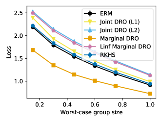
Figure 8: Comparison of various smoothness assumptions on the conditional risk on the wine quality prediction dataset.

Appendix B Risk bounds under confounding

Our assumption that $P_{Y\mid X}$ is fixed for each of our marginal populations over $X$ is analogous to the frequent assumptions in causal inference that there are no unmeasured confounders [44]. When this is true—for example, in machine learning tasks where the label $Y$ is a human annotation of the covariate $X$—minimizing worst-case loss over covariate shifts is natural, but the assumption may fail in other real-world problems. For example, in predicting crime recidivism $Y$ based on the type $X$ of crime committed and race $Z$ of the individual, unobserved confounders $C$ (e.g. income, location, education) likely vary with race. Consequently, we provide a parallel to our earlier development that provides a sensitivity analysis to unmeasured (hidden) confounding.

Let us formalize. Let $C\in\mathcal{C}$ be a random variable, and in analogy to (2) we define

$$\mathcal{P}_{\alpha_{0},(X,C)}:=\left\{Q_{0}:\exists~{}\alpha\geq\alpha_{0}~{}\mbox{and~{}measure}~{}Q_{1}~{}\mbox{on}~{}(\mathcal{X}\times\mathcal{C})~{}\mbox{s.t.}~{}P_{(X,C)}=\alpha Q_{0}+(1-\alpha)Q_{1}\right\}.$$ (29)

Our goal is then to minimize the worst-case loss under mixture covariate shifts

$$\mathop{\rm minimize}_{\theta\in\Theta}\sup_{Q_{0}\in\mathcal{P}_{\alpha_{0},(X,C)}}\underset{(X,C)\sim Q_{0}}{\mathbb{E}}[\mathbb{E}[\ell(\theta;(X,Y))\mid X,C]].$$ (30)

Since the confounding variable $C$ is unobserved, we extend our robustness approach assuming a bounded effect of confounding, and derive conservative upper bounds on the worst-case loss.

We make the following boundedness definition and assumption on the effects of $C$.

Definition 1.

The triple $(X,Y,C)$ is at most $\delta$-confounded for the loss $\ell$ if

$$\left\|{\mathbb{E}[\ell(\theta;(X,Y))\mid X]-\mathbb{E}[\ell(\theta;(X,Y))\mid X,C]}\right\|_{L^{\infty}(P)}\leq\delta.$$

Assumption A4.

The triple $(X,Y,C)$ is at most $\delta$-confounded for the loss $\ell$.

Paralleling earlier developments, we derive a variational bound on the worst-case confounded risk (30). If $C=Y$, our worst-case formulation approaches the joint DRO problem as $\delta\to\infty$.

Confounded variational problem

Under confounding, a development completely parallel to Lemma 2.1 and Hölder’s inequality yields the dual

$$\sup_{Q_{0}\in\mathcal{P}_{\alpha_{0},(X,C)}}\underset{(X,C)\sim Q_{0}}{\mathbb{E}}[\mathbb{E}[\ell(\theta;(X,Y))\mid X,C]]$$

$$\leq\inf_{\eta\in\mathbb{R}}\left\{\frac{1}{\alpha_{0}}\left(\mathbb{E}_{(X,C)\sim P_{(X,C)}}\left[\left({\mathbb{E}[\ell(\theta;(X,Y))\mid X,C]-\eta}\right)_{+}^{{p}}\right]\right)^{\frac{1}{{p}}}+\eta\right\}$$

for all ${p}\geq 1$. Taking the variational form of the $L^{p}$-norm for $p\in\left({1},{2}\right]$ yields

$$\begin{split}&\left(\mathbb{E}_{P_{X,C}}\left[\left({\mathbb{E}[\ell(\theta;(X,Y))\mid X,C]-\eta}\right)_{+}^{p}\right]\right)^{{1/p}}\\ &=\sup_{h}\left\{\mathbb{E}\left[h(X,C)(\mathbb{E}[\ell(\theta;(X,Y))\mid X,C]-\eta)\right]~{}\Big{|}~{}h\geq 0,\mathbb{E}[h^{q}(X,C)]\leq 1\right\}.\end{split}$$ (31)

Instead of the somewhat challenging variational problem over $h$, we reparameterize problem (31) as $h(X)+f(X,C)$, where $h$ is smooth and $f$ is a bounded residual term, which—by taking the worst case over bounded $f$—allows us to provide an upper bound on the worst-case problem (29). Let $\mathcal{H}_{L,{p}}$ be the space of Hölder functions (11) and $\mathcal{F}_{\delta,{p}}$ be the space of bounded functions

$$\mathcal{F}_{\delta,{p}}:=\left\{f:\mathcal{X}\times\mathcal{C}\to\mathbb{R}~{}\mbox{measurable},~{}\left\|{f(X,C)}\right\|_{L^{\infty}(P)}\leq\delta^{{p}-1}\right\}.$$

Then defining the analogue of the unconfounded variational objective (12)

$$R_{{p},\epsilon,L,\delta}(\theta,\eta):=\sup_{h+f\geq 0}\left\{\mathbb{E}\left[\frac{h(X)+f(X,C)}{\epsilon}(\ell(\theta;(X,Y))-\eta)\right]\mid h\in\mathcal{H}_{L,{p}},f\in\mathcal{F}_{\delta,{p}},\left\|{h+f}\right\|_{L^{q}(P)}\leq\epsilon\right\},$$

the risk $R_{{p},\epsilon,L,\delta}$ is $\epsilon$-close to the variational objective (31). See Appendix D.12 for proof.

Lemma B.1.

Let Assumptions A1, A3, and A4 hold. Then, for any $\theta\in\Theta$ and $\eta\in\mathbb{R}$, we have

$$\left(\mathbb{E}_{P_{X,C}}\left[\left({\mathbb{E}[\ell(\theta;(X,Y))\mid X,C]-\eta}\right)_{+}^{p}\right]\right)^{{1/p}}=\inf_{\epsilon\geq 0}\left\{R_{{p},\epsilon,L,\delta}(\theta,\eta)\vee\epsilon^{q-1}\right\}$$ (32)

and for any $\epsilon>0$, $(R_{{p},\epsilon,L,\delta}(\theta,\eta)\vee\epsilon^{q-1})-\epsilon^{q-1}\leq\left(\mathbb{E}_{P_{X,C}}\left[\left({\mathbb{E}[\ell(\theta;(X,Y))\mid X,C]-\eta}\right)_{+}^{p}\right]\right)^{{1/p}}.$

Confounded estimator

By replacing $\mathcal{H}_{L,{p}}$ with the empirical version $\widehat{\mathcal{H}}_{L,{p}}$ (the set of Hölder functions on the empirical distribution) and $\mathcal{F}_{\delta,{p}}$ with the empirical counterpart $\mathcal{F}_{\delta,p,n}:=\{f\in\mathbb{R}^{n}\mid\max_{i\leq n}|f(X_{i},C_{i})|\leq\delta^{p-1}\}$, we get the obvious empirical plug-in $\widehat{R}_{{p},\epsilon,L,\delta}(\theta,\eta)$ of the population quantity $R_{{p},\epsilon,L,\delta}(\theta,\eta)$. In this case, a duality argument provides the following analogue of Lemma 4.1, which follows because the class $\mathcal{F}_{\delta,p,n}$ simply corresponds to an $\left\|{\cdot}\right\|_{\infty}$ constraint on a vector in $\mathbb{R}^{n}$.

Lemma B.2.

For any $\epsilon>0$ and $(X_{1},Y_{1}),\ldots,(X_{n},Y_{n})$, we have

$$\widehat{R}_{{p},\epsilon,L,\delta}(\theta,\eta) =\inf_{B\in\mathbb{R}^{n\times n}_{+}}\Bigg{\{}\bigg{(}\frac{{p}-1}{n}\sum_{i=1}^{n}\Big{(}{\ell(\theta;(X_{i},Y_{i}))-\frac{1}{n}\sum_{j=1}^{n}(B_{ij}-B_{ji})-\eta}\Big{)}_{+}^{p}\bigg{)}^{{1/p}}$$

$$\hskip 80.0pt+\frac{L^{{p}-1}}{\epsilon n^{2}}\sum_{i,j=1}^{n}\left\|{X_{i}-X_{j}}\right\|B_{ij}+\frac{2\delta^{{p}-1}}{\epsilon n^{2}}\sum_{i,j=1}^{n}|B_{ij}|\Bigg{\}}.$$

See Appendix D.14 for the proof. The lemma is satisfying in that it smoothly interpolates, based on the degree of confounding $\delta$, between marginal distributionally robust optimization (when $\delta=0$, as in Lemma 4.1) and the fully robust joint DRO setting as $\delta\uparrow\infty$, which results in the choice $B=0$.

Upper bound on confounded objective

In analogy with Proposition 2, the empirical plug-in $\widehat{R}_{{p},\epsilon,L,\delta}(\theta,\eta)$ is an upper bound on the population objective under confounding. Although our estimator only provides an upper bound, it provides practical procedures for controlling the worst-case loss (29) when Assumption A4 holds, as we observe in the next section. The next proposition, whose proof we provide in Section D.13, shows the upper bound.

Proposition 3.

Let Assumptions A1, A3, and A4 hold. There exist universal constants $c_{1},c_{2}<\infty$ such that the following holds. Let $\theta\in\Theta$, $\epsilon>0$, and ${p}\in\left({1},{2}\right]$. Then with probability at least $1-2\gamma$, uniformly in $\eta\in[0,M]$

$$\left(\mathbb{E}_{P_{X,C}}\left({\mathbb{E}[\ell(\theta;(X,Y))\mid X,C]-\eta}\right)_{+}^{p}\right)^{{1/p}}$$

$$\leq\max\left\{\epsilon^{q-1},~{}(1+\tau_{n}(\gamma,\epsilon))^{{1/q}}~{}\widehat{R}_{{p},\epsilon,L_{n}(\gamma),\delta_{n}(\gamma)}(\theta,\eta)+\frac{c_{1}M^{2}}{\epsilon^{q-1}}\sqrt{\frac{\log\frac{1}{\gamma}}{n}}\right\}$$

where $\tau_{n}(\gamma,\epsilon):=\frac{c_{2}M^{2}}{\epsilon^{q-1}}\sqrt{\frac{1}{n}\log\frac{1}{\gamma}}$, $\delta_{n}(\gamma):=\delta(1+\tau_{n}(\gamma,\epsilon))^{-{1/q}}$, and $L_{n}(\gamma):=L(1+\tau_{n}(\gamma,\epsilon))^{-{1/q}}$.

B.1 Simulation study: the confounded case

To complement our results in the unconfounded case, we extend our simulation experiment by adding unmeasured confounders, investigating the risk upper bounds of Lemma B.2 and Proposition 3. We generate data nearly identically to model (28), introducing a confounder $C$:

$$Z\sim\mathsf{Bern}(0.15),~{}~{} X_{1}=(1-2Z)\cdot\mathsf{Uni}([0,1]),~{}~{}X_{2},\ldots,X_{d}\stackrel{{\scriptstyle\rm iid}}{{\sim}}\mathsf{Uni}([0,1])$$

$$Y=|X_{1}|+\mathbf{1}\left\{X_{1}\geq 0\right\}\cdot C,~{}~{}C\sim\mathsf{Uni}(\{-1,0.5,0,0.5,1\}).$$

To evaluate a putative parameter $\theta$, we approximate the worst-case risk

$$R_{\alpha_{0}}(\theta,c):=\sup_{Q_{0}\in\mathcal{P}_{\alpha_{0},X}}\underset{X\sim Q_{0}}{\mathbb{E}}\mathbb{E}\left[|\theta^{\top}X-Y|\mid X,C=c\right].$$ (33)

via the plug-in replicate estimate in Proposition 1, using a sample of size $n=2000$, $m=10$ replicates, and test-time worst-case group size $\alpha_{0}=0.05$. The gap in the conditional risk from $\delta$-confounding (i.e. $\mathbb{E}[\ell(\theta;(X,Y))\mid X]-\mathbb{E}[\ell(\theta;(X,Y))\mid X,C]$) in Definition 1 varies monotonically with $|c|$. To construct estimates $\widehat{\theta}$, we minimize the dual representation of the empirical confounded risk $\widehat{R}_{{p},\epsilon,L,\delta}(\theta,\eta)$ in Lemma B.2, varying the postulated level $\delta$ of confounding while fixing the training time worst-case group size $\alpha_{0}=0.1$. We present results in Fig. 9, which compares the worst-case loss (33) as $c$ varies (vertical axis) for different methods to select $\widehat{\theta}$ (horizontal axis). We compare marginal DRO (16) (which assumes no confounding $\delta=0$), the procedure minimizing empirical confounded risk $\widehat{R}_{{p},\epsilon,L,\delta}(\theta,\eta)$ as we vary $\delta$, and the joint DRO procedure (21) (full confounding) with $p=1,2$, and empirical risk minimization (ERM). The figure shows the (roughly) expected result that the confounding-aware risks achieve lower worst-case loss (33) as the postulated confounding level $\delta$ increases with the actual amount of confounding, with joint DRO and ERM achieving worse performance.

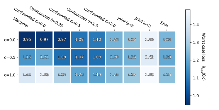
Figure 9: Worst-case losses (Eq. 33) incurred by each model (column) when varying the influence of the unobserved confounder $c$ (rows). Adjusting marginal DRO to account for the level of confounding (Lemma B.2) by varying $\delta$ improves worst-case loss.

Appendix C Additional validation experiments

In this section, we provide additional experiments quantifying the computational overhead associated with marginal DRO, and analyze the robustness of previous results with respect to the choice of the loss function. Finally, we compare different smoothness assumptions on the conditional risk on real-world data.

C.1 Computational overhead

To analyze the computational overhead of marginal DRO, we benchmark both the number of gradient oracle calls (defined as the number of times we take the gradient of the objective with respect to $\theta$ or $B$) and overall runtime. We focus on the simulation experiments in Section 6.1 with $d=10$ and $n=100$. The results in Figure 10 show that marginal DRO incurs a 2-3x overhead, but the overall runtime costs of all algorithms are still low. The gradient call comparisons show that the increased runtimes are primarily due to the increased cost of individual gradient calls (as each gradient computation for marginal DRO involves gradients over both the model parameters $\theta$ as well as the transport matrix $B$) rather then increases in the number of overall gradient steps.

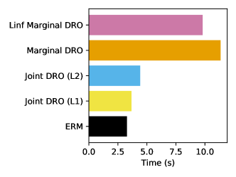
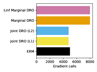
Figure 10: Runtime costs of marginal DRO and baselines

All DRO methods including joint and marginal DRO use bisection search to optimize the dual parameter $\eta$, but this additional cost does not substantially affect the number of gradient calls or runtime, as we re-use initializations for gradient descent across different steps of the bisection search. The added number of gradient calls to marginal DRO methods arise from the fact that we must tune one additional hyperparameter $(L/\epsilon)$ which involves additional grid search on top of the bisection search.

There is an added $2\times$ gradient call overhead for the marginal DRO variants, which must additionally perform hyperparameter search over $L/\epsilon$ on a held out set. Even with re-using initializations, this results in a higher number of gradient oracle calls. Finally, there is an additional runtime overhead for both marginal DRO variants in terms of runtime due to the larger number of parameters.

C.2 Effect of loss function choice

We also quantify the impact of the loss function by re-running the large scale simulation in Figure 2 using the squared loss rather than the absolute deviation loss, keeping the same experimental settings such as validation methods and hyperparameters. We find in Figure 11 that the results in the simulation remain qualitatively same as before. The main difference is that $L_{\infty}$ marginal DRO performs slightly better, but none of the ERM or joint DRO baselines perform well even in this setting. Together with the classification results discussed in previous sections, these squared loss results suggest that the performance gains of marginal DRO are not limited to minimizing the absolute deviation loss.

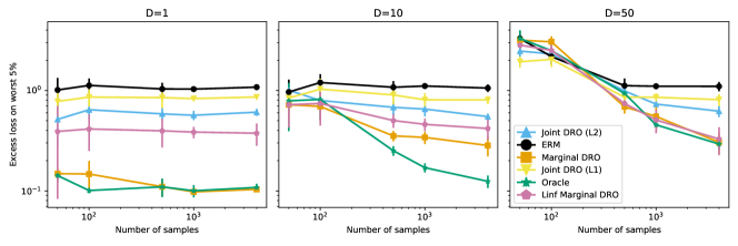
Figure 11: Simulation experiments with the squared loss rather than absolute deviation loss

Appendix D Proofs

D.1 Proof of Lemma 2.1

We begin by deriving a likelihood ratio reformulation, where we use $W:=\mathbb{E}[\ell(\theta;(X,Y))\mid X]$ to ease notation

$$\sup_{Q_{0}\in\mathcal{P}_{\alpha_{0},X}}\mathbb{E}_{X\sim Q_{0}}[W]=\sup_{L}\left\{\mathbb{E}_{P}[LW]\Bigg{|}L:\Omega\to[0,1/\alpha_{0}],~{}\mbox{measurable},~{}\mathbb{E}_{p}[L]=1\right\}.$$ (34)

To see that inequality “$\leq$” holds, let $Q_{0}\in\mathcal{P}_{\alpha_{0},X}$ be a probability over $\mathcal{X}$. Note that $Q_{0}$ induces a distribution over $(\Omega,\sigma(X))$, which we denote by the same notation for simplicity. Since $P_{X}=\alpha_{0}Q_{0}+(1-\alpha_{0})Q_{1}$ for some probability $Q_{1}$ and $\alpha_{0}\in(0,1)$, we have $Q_{0}\ll P_{X}$. Letting $L:=\frac{dQ_{0}}{dP_{X}}$, it belongs to the constraint set in the right hand side and we conclude $\leq$ holds. To see the reverse inequality “$\geq$”, for any likelihood ratio $L:\Omega\to[0,1/\alpha_{0}]$, let $Q_{0}:=P_{X}L$ so that $Q_{0}(A):=\mathbb{E}_{P_{X}}[\mathbf{1}\left\{A\right\}L]$ for all $A\in\sigma(X)$. Noting $Q_{1}:=\frac{1}{1-\alpha_{0}}P_{X}-\frac{\alpha_{0}}{1-\alpha_{0}}Q_{0}$ defines a probability measure and $P_{X}=\alpha_{0}Q_{0}+(1-\alpha_{0})Q_{1}$, we conclude that inequality $\geq$ holds.

Next, the following lemma gives a variational form for conditional value-at-risk, which corresponds to the worst-case loss (2) under mixture covariate shifts.

Lemma D.1 ([70, Example 6.19]).

For any random variable $W:\mathcal{X}\to\mathbb{R}$ with $\mathbb{E}|W|<\infty$,

$$\sup_{L}\left\{\mathbb{E}_{P}[LW]\Bigg{|}L:\Omega\to[0,\frac{1}{\alpha_{0}}],~{}\mbox{measurable},~{}\mathbb{E}_{p}[L]=1\right\}$$

$$=\inf_{\eta\in\mathbb{R}}\left\{\frac{1}{\alpha_{0}}\mathbb{E}_{X\sim P_{X}}\left[\left({W-\eta}\right)_{+}\right]+\eta\right\}.$$

From the reformulation (34) and Lemma D.1, we obtain the first result.

We now show that when $W\in[0,M]$,

$$\inf_{\eta\in\mathbb{R}}\left\{\frac{1}{\alpha_{0}}\mathbb{E}[\left({W-\eta}\right)_{+}]+\eta\right\}=\inf_{\eta\in[0,M]}\left\{\frac{1}{\alpha_{0}}\mathbb{E}[\left({W-\eta}\right)_{+}]+\eta\right\}.$$ (35)

Noting that $\eta\mapsto g(\eta):=\frac{1}{\alpha_{0}}\mathbb{E}[\left({W-\eta}\right)_{+}]+\eta$ is strictly increasing on $\left[{M},{\infty}\right)$ since $g(\eta)=\eta$ for $\eta\in\left[{M},{\infty}\right)$, we may assume w.l.o.g. that $\eta\leq M$. Further, for $\eta\leq 0$, we have

$$g(\eta)=\frac{1}{\alpha_{0}}\mathbb{E}[W]+\left(\frac{1}{\alpha_{0}}-1\right)|\eta|\geq\frac{1}{\alpha_{0}}\mathbb{E}[W]=g(0).$$

We conclude that the equality (35) holds.

D.2 Proof of Proposition 1

Using the dual of Lemma 2.1, we first show that with probability at least $1-\gamma$,

$$\sup_{\eta\in[0,M]}\Bigg{|}\mathbb{E}_{X\sim P_{X}}\left[\left({\mathbb{E}[\ell(\theta;(X,Y))\mid X]-\eta}\right)_{+}\right]-\frac{1}{n}\sum_{i=1}^{n}\bigg{(}{\frac{1}{m}\sum_{j=1}^{m}\ell(\theta;(X_{i},Y_{i,j}))-\eta}\bigg{)}_{+}\Bigg{|}$$

$$\leq CM\sqrt{\frac{1+\log\frac{1}{\gamma}}{\min\{m,n\}}}.$$ (36)

As the above gives a uniform approximation to the dual objective $\frac{1}{\alpha_{0}}\mathbb{E}[\left({\mathbb{E}[\ell(\theta;(X,Y))\mid X]-\eta}\right)_{+}]+\eta$, the proposition will then follow.

To show the result (36), we begin by noting that

$$\sup_{\eta\in[0,M]}\Bigg{|}\mathbb{E}_{X\sim P_{X}}\left[\left({\mathbb{E}[\ell(\theta;(X,Y))\mid X]-\eta}\right)_{+}\right]-\frac{1}{n}\sum_{i=1}^{n}\bigg{(}{\frac{1}{m}\sum_{j=1}^{m}\ell(\theta;(X_{i},Y_{i,j}))-\eta}\bigg{)}_{+}\Bigg{|}$$

$$\leq\sup_{\eta\in[0,M]}\Bigg{|}\mathbb{E}_{X\sim P_{X}}\left[\left({\mathbb{E}[\ell(\theta;(X,Y))\mid X]-\eta}\right)_{+}\right]-\frac{1}{n}\sum_{i=1}^{n}\left({\mathbb{E}[\ell(\theta;(X_{i},Y))\mid X=X_{i}]-\eta}\right)_{+}\Bigg{|}$$

$$\qquad+\sup_{\eta\in[0,M]}\frac{1}{n}\sum_{i=1}^{n}\bigg{|}\left({\mathbb{E}[\ell(\theta;(X_{i},Y))\mid X=X_{i}]-\eta}\right)_{+}-\bigg{(}{\frac{1}{m}\sum_{j=1}^{m}\ell(\theta;(X_{i},Y_{i,j}))-\eta}\bigg{)}_{+}\bigg{|}.$$ (37)

To bound the first term in the bound (37), note that since $\eta\mapsto\left({Z-\eta}\right)_{+}$ is $1$-Lipschitz, a standard symmetrization and Rademacher contraction argument [18, 7] yields

$$\sup_{\eta\in[0,M]}\Bigg{|}\mathbb{E}\left[\left({\mathbb{E}[\ell(\theta;(X,Y))\mid X]-\eta}\right)_{+}\right]-\frac{1}{n}\sum_{i=1}^{n}\left({\mathbb{E}[\ell(\theta;(X_{i},Y))\mid X=X_{i}]-\eta}\right)_{+}\Bigg{|}\leq C\sqrt{\frac{M^{2}}{n}(1+t)}$$

with probability at least $1-e^{-t}$. To bound the second term in the bound (37), we first note that

$$\sup_{\eta\in[0,M]}\left|\left({\mathbb{E}[\ell(\theta;(X,Y))\mid X=X_{i}]-\eta}\right)_{+}-\bigg{(}{\frac{1}{m}\sum_{j=1}^{m}\ell(\theta;(X_{i},Y_{i,j}))-\eta}\bigg{)}_{+}\right|$$

$$\leq\left|\mathbb{E}[\ell(\theta;(X_{i},Y_{i,j}))\mid X=X_{i}]-\frac{1}{m}\sum_{j=1}^{m}\ell(\theta;(X_{i},Y_{i,j}))\right|$$

since $|\left({x-\eta}\right)_{+}-\left({x^{\prime}-\eta}\right)_{+}|\leq|x-x^{\prime}|$. The preceding quantity has bound $M$, and using that its expectation is at most $M/\sqrt{m}$ the bounded differences inequality implies the uniform concentration result (36).

The second result follows from a nearly identical argument by noting that we still have the Lipschitz relation

$$|\left({\mathbb{E}[\ell(\theta;X,Y)\mid X]-\eta}\right)_{+}-\left({\mathbb{E}[\ell(\theta^{\prime};X,Y)\mid X]-\eta^{\prime}}\right)_{+}|\leq K\left\|{\theta-\theta^{\prime}}\right\|_{2}+|\eta-\eta^{\prime}|.$$

D.3 Proof of Lemma A.1

Let $\mathcal{L}_{\alpha_{0}}:=\{h:\mathcal{X}\to\mathbb{R}_{+}\mid\mathbb{E}_{P}[h(X)]=\alpha_{0}\}$. Since $\frac{dQ_{0}}{dP}$ is a likelihood ratio and $\mathbb{E}[dQ_{0}/dP]=1$, we have the upper bound

$$\mathbb{E}_{X\sim Q_{0}}[\mathbb{E}[\ell(\theta;(X,Y))\mid X]]=\mathbb{E}_{P}\left[\frac{dQ_{0}(X)}{dP(X)}\ell(\theta;(X,Y))\right]\leq\sup_{h\in\mathcal{H}_{L,2}\cap\mathcal{L}_{\alpha_{0}}}\mathbb{E}_{P}\left[\frac{h(X)}{\alpha_{0}}\ell(\theta;(X,Y))\right].$$

Then we use the sequence of inequalities, starting from our dual representation on $\mathcal{R}_{L,2}$, that

$$\mathcal{R}_{L,2}(\theta) =\inf_{\eta}\sup_{h\in\mathcal{H}_{L,2}}\frac{1}{\alpha_{0}}\mathbb{E}_{P}\left[h(X)(\ell(\theta;(X,Y))-\eta)\right]+\eta$$

$$\geq\sup_{h\in\mathcal{H}_{L,2}}\inf_{\eta}\frac{1}{\alpha_{0}}\mathbb{E}_{P}\left[h(X)(\ell(\theta;(X,Y))-\eta)\right]+\eta$$

$$\geq\sup_{h\in\mathcal{H}_{L,2}\cap\mathcal{L}_{\alpha_{0}}}\frac{1}{\alpha_{0}}\mathbb{E}_{P}\left[h(X)(\ell(\theta;(X,Y))-\eta)\right]+\eta=\sup_{h\in\mathcal{H}_{L,2}\cap\mathcal{L}_{\alpha_{0}}}\mathbb{E}_{P}[h(X)\ell(\theta;(X,Y))].$$

This gives the result.

D.4 Proof of Lemma 3.1

Since $Z,\eta\in[0,M]$, we have

$$\mathbb{E}_{X\sim P_{X}}\left[\left({Z(X)-\eta}\right)_{+}^{p}\right]\leq(M-\eta)^{{p}-1}\mathbb{E}_{X\sim P_{X}}\left[\left({Z(X)-\eta}\right)_{+}\right]$$

which gives the first bound. To get the second bound, note that for a $L$-Lipschitz function $f$, we have $\mathbb{E}[f(X)]\leq f(\mathbb{E}[X])+L\mathbb{E}|X-\mathbb{E}[X]|$. Since $f(x)=x^{p}$ is ${p}(M-\eta)^{{p}-1}$-Lipschitz on $[0,M-\eta]$, we get

$$\mathbb{E}_{X\sim P_{X}}\left[\left({Z(X)-\eta}\right)_{+}^{p}\right]\leq\left(\mathbb{E}_{X\sim P_{X}}\left[\left({Z(X)-\eta}\right)_{+}\right]\right)^{p}+{p}(M-\eta)^{{p}-1}\mathbb{E}\left|\left({Z(X)-\eta}\right)_{+}-\mathbb{E}[\left({Z(X)-\eta}\right)_{+}]\right|.$$

Taking $1/{p}$-power on both sides, we obtain the second bound.

D.5 Proof of Lemma 3.2

First, we argue that

$$\sup_{h}\left\{\mathbb{E}\left[h(X)(\ell(\theta;(X,Y))-\eta)\right]~{}~{}\Big{|}~{}~{}h:\mathcal{X}\to\mathbb{R}_{+},~{}\mathbb{E}[h^{q}(X)]\leq 1\right\}$$

$$\leq\sup_{h\in\mathcal{H}_{L,{p}}}\left\{\mathbb{E}\left[\frac{h(X)}{\epsilon}(\ell(\theta;(X,Y))-\eta)\right]\vee\epsilon^{q-1}~{}~{}\Bigg{|}~{}~{}h\geq 0,~{}\left(\mathbb{E}[h^{q}(X)]\right)^{{1/q}}\leq\epsilon\right\}$$ (38)

and for any $\epsilon>0$. We consider an arbitrary but fixed $\theta$ and $\eta$.

Suppose that $\epsilon^{q-1}\geq\left(\mathbb{E}_{X\sim P_{X}}\left[\left({\mathbb{E}[\ell(\theta;(X,Y))\mid X]-\eta}\right)_{+}^{p}\right]\right)^{{1/p}}$, then

$$\epsilon^{q-1} \geq\left(\mathbb{E}_{X\sim P_{X}}\left[\left({\mathbb{E}[\ell(\theta;(X,Y))\mid X]-\eta}\right)_{+}^{p}\right]\right)^{{1/p}}$$

$$=\sup_{h}\left\{\mathbb{E}\left[h(X)(\mathbb{E}[\ell(\theta;(X,Y))\mid X]-\eta)\right]~{}~{}\Big{|}~{}~{}h:\mathcal{X}\to\mathbb{R}~{}\mbox{measurable},~{}h\geq 0,~{}\mathbb{E}[h^{q}(X)]\leq 1\right\}$$

$$\geq\sup_{h\in\mathcal{H}_{L,{p}}}\left\{\mathbb{E}\left[\frac{h(X)}{\epsilon}(\mathbb{E}[\ell(\theta;(X,Y))\mid X]-\eta)\right]:~{}h\geq 0,~{}\left(\mathbb{E}[h^{q}(X)]\right)^{{1/q}}\leq\epsilon\right\},$$

and we have the upper bound. On the other hand, assume $\epsilon^{q-1}\leq\left(\mathbb{E}_{X\sim P_{X}}\left[\left({\mathbb{E}[\ell(\theta;(X,Y))\mid X]-\eta}\right)_{+}^{p}\right]\right)^{{1/p}}$. The inner supremum in Eq. (9) is attained at $h^{\star}$ defined in expression (10), and from Assumption A3, for any $x,x^{\prime}\in\mathcal{X}$,

$$|h^{\star}(x)-h^{\star}(x^{\prime})| \leq\frac{1}{\epsilon}\left|\left({\mathbb{E}[\ell(\theta;(X,Y))\mid X=x]-\eta}\right)_{+}^{{p}-1}-\left({\mathbb{E}[\ell(\theta;(X,Y))\mid X=x^{\prime}]-\eta}\right)_{+}^{{p}-1}\right|$$

$$\leq\frac{1}{\epsilon}\left|\left({\mathbb{E}[\ell(\theta;(X,Y))\mid X=x]-\eta}\right)_{+}-\left({\mathbb{E}[\ell(\theta;(X,Y))\mid X=x^{\prime}]-\eta}\right)_{+}\right|^{{p}-1}$$

$$\leq\frac{1}{\epsilon}\left|\mathbb{E}[\ell(\theta;(X,Y))\mid X=x]-\mathbb{E}[\ell(\theta;(X,Y))\mid X=x^{\prime}]\right|^{{p}-1}$$

$$\leq\frac{L^{{p}-1}}{\epsilon}\left\|{x-x^{\prime}}\right\|^{{p}-1},$$

where we used $\epsilon\leq\left(\mathbb{E}_{X\sim P_{X}}\left[\left({\mathbb{E}[\ell(\theta;(X,Y))\mid X]-\eta}\right)_{+}^{p}\right]\right)^{{1/q}}$ in the first inequality. Thus, we conclude that $\epsilon h^{\star}$ is in $\mathcal{H}_{L,{p}}$, and obtain the equality

$$\left(\mathbb{E}_{X\sim P_{X}}\left[\left({\mathbb{E}[\ell(\theta;(X,Y))\mid X]-\eta}\right)_{+}^{p}\right]\right)^{{1/p}}$$

$$=\sup_{h}\left\{\mathbb{E}_{X\sim P_{X}}\left[(\mathbb{E}[\ell(\theta;(X,Y))\mid X]-\eta)h(X)\right]\Bigg{|}h:\mathcal{X}\to\mathbb{R}~{}\mbox{measurable},~{}h\geq 0,~{}\mathbb{E}[h^{q}(X)]\leq 1,~{}\mbox{and}~{}\epsilon h\in\mathcal{H}_{L,{p}}\right\}$$

$$=\sup_{h\in\mathcal{H}_{L,{p}}}\left\{\mathbb{E}\left[\frac{h(X)}{\epsilon}(\ell(\theta;(X,Y))-\eta)\right]~{}~{}\Bigg{|}~{}~{}h\geq 0,~{}\left(\mathbb{E}[h^{q}(X)]\right)^{{1/q}}\leq\epsilon\right\}$$

where we did a change of variables $h$ to $h/\epsilon$ in the last equality. This yields the bound (38).

Now, for $\epsilon=\left(\mathbb{E}_{X\sim P_{X}}\left[\left({\mathbb{E}[\ell(\theta;(X,Y))\mid X]-\eta}\right)_{+}^{p}\right]\right)^{{1/q}}$, the bound (38) is actually an equality. This proves the first claim. To show the second claim, it remains to show that

$$\sup_{h\in\mathcal{H}_{L,{p}}}\left\{\mathbb{E}\left[\frac{h(X)}{\epsilon}(\ell(\theta;(X,Y))-\eta)\right]\vee\epsilon^{q-1}~{}~{}\Bigg{|}~{}~{}h\geq 0,~{}\left(\mathbb{E}[h^{q}(X)]\right)^{{1/q}}\leq\epsilon\right\}-\epsilon^{q-1}$$

$$\leq\sup_{h}\left\{\mathbb{E}\left[h(X)(\ell(\theta;(X,Y))-\eta)\right]~{}~{}\Big{|}~{}~{}h:\mathcal{X}\to\mathbb{R},~{}\mbox{measurable},~{}h\geq 0,~{}\mathbb{E}[h^{q}(X)]\leq 1\right\}.$$

If $\epsilon^{q-1}\geq\left(\mathbb{E}_{X\sim P_{X}}\left[\left({\mathbb{E}[\ell(\theta;(X,Y))\mid X]-\eta}\right)_{+}^{p}\right]\right)^{{1/p}}$, then the left hand side is less than or equal to $0$ by the same logic above. If $\epsilon^{q-1}\leq\left(\mathbb{E}_{X\sim P_{X}}\left[\left({\mathbb{E}[\ell(\theta;(X,Y))\mid X]-\eta}\right)_{+}^{p}\right]\right)^{{1/p}}$, then we have

$$\sup_{h\in\mathcal{H}_{L,{p}}}\left\{\mathbb{E}\left[\frac{h(X)}{\epsilon}(\ell(\theta;(X,Y))-\eta)\right]\vee\epsilon^{q-1}~{}~{}\Bigg{|}~{}~{}h\geq 0,~{}\left(\mathbb{E}[h^{q}(X)]\right)^{{1/q}}\leq\epsilon\right\}$$

$$=\sup_{h}\left\{\mathbb{E}\left[h(X)(\ell(\theta;(X,Y))-\eta)\right]~{}~{}\Big{|}~{}~{}h:\mathcal{X}\to\mathbb{R},~{}\mbox{measurable},~{}h\geq 0,~{}\mathbb{E}[h^{q}(X)]\leq 1\right\},$$

so the result follows.

D.6 Proof of Lemma 4.1

We take the dual of the following optimization problem

$$\mathop{\rm maximize}_{h\in\mathbb{R}^{n}}~{}~{}\frac{1}{n}\sum_{i=1}^{n}\frac{h_{i}}{\epsilon}(\ell(\theta;(X_{i},Y_{i}))-\eta)$$

$$\mathop{\rm subject\;to}~{}~{}h_{i}\geq 0~{}~{}\mbox{for all}~{}~{}i\in[n],~{}~{}\frac{1}{n}\sum_{i=1}^{n}h_{i}^{q}\leq\epsilon^{q},$$

$$\hskip 45.0pt~{}~{}h_{i}-h_{j}\leq L^{{p}-1}\left\|{X_{i}-X_{j}}\right\|^{{p}-1}~{}~{}\mbox{for all}~{}~{}i,j\in[n]$$

where $h_{i}:=h(X_{i})$. To ease notation, we do a change of variables $h_{i}\leftarrow\frac{h_{i}}{\epsilon}$

$$\mathop{\rm maximize}_{h\in\mathbb{R}^{n}}~{}~{}\frac{1}{n}\sum_{i=1}^{n}h_{i}(\ell(\theta;(X_{i},Y_{i}))-\eta)$$ (39)

$$\mathop{\rm subject\;to}~{}~{}h_{i}\geq 0~{}~{}\mbox{for all}~{}~{}i\in[n],~{}~{}\frac{1}{n}\sum_{i=1}^{n}h_{i}^{q}\leq 1,$$

$$\hskip 45.0pt~{}~{}h_{i}-h_{j}\leq\frac{L^{{p}-1}}{\epsilon}\left\|{X_{i}-X_{j}}\right\|^{{p}-1}~{}~{}\mbox{for all}~{}~{}i,j\in[n].$$

For $\gamma\in\mathbb{R}^{n}_{+}$, $\lambda\geq 0$, $B\in\mathbb{R}^{n\times n}_{+}$, the associated Lagrangian is given by

$$\mathcal{L}(h,\gamma,\lambda,B) :=\frac{1}{n}\sum_{i=1}^{n}h_{i}(\ell(\theta;(X_{i},Y_{i}))-\eta)+\gamma^{\top}h+\frac{\lambda}{q}\left(1-\frac{1}{n}\sum_{i=1}^{n}h_{i}^{q}\right)$$

$$\qquad+\frac{1}{n^{2}}\left(\frac{L^{{p}-1}}{\epsilon}\mathop{\rm tr}(B^{\top}D)-h^{\top}(B\mathbbm{1}-B^{\top}\mathbbm{1})\right)$$

where $D\in\mathbb{R}^{n\times n}$ is a matrix with entries $D_{ij}=\left\|{X_{i}-X_{j}}\right\|^{{p}-1}$. From strong duality, we have that the primal optimal value (39) is equal to $\inf_{\gamma\in\mathbb{R}^{n}_{+},\lambda\geq 0,B\in\mathbb{R}^{n\times n}_{+}}\sup_{h}\mathcal{L}(h,\gamma,\lambda,B)$.

Since $h\mapsto\mathcal{L}(h,\gamma,\lambda,B)$ is a quadratic, a bit of algebra shows that

$$\sup_{h}\mathcal{L}(h,\gamma,\lambda,B)=\frac{\lambda}{q}+\frac{L^{{p}-1}}{\epsilon n^{2}}\mathop{\rm tr}(B^{\top}D)+\frac{1}{q\lambda^{{p}-1}n}\sum_{i=1}^{n}\left(\ell(\theta;(X_{i},Y_{i}))-\eta-\frac{1}{n}(B\mathbbm{1}-B^{\top}\mathbbm{1})_{i}+\gamma_{i}\right)^{p}.$$

From complementary slackness,

$$\inf_{\gamma\in\mathbb{R}^{n}_{+}}\sup_{h}\mathcal{L}(h,\gamma,\lambda,B)=\frac{\lambda}{q}+\frac{L^{{p}-1}}{\epsilon n^{2}}\mathop{\rm tr}(B^{\top}D)+\frac{1}{q\lambda^{{p}-1}n}\sum_{i=1}^{n}\left({\ell(\theta;(X_{i},Y_{i}))-\eta-\frac{1}{n}(B\mathbbm{1}-B^{\top}\mathbbm{1})_{i}}\right)_{+}^{p}.$$

Finally, taking infimum with respect to $\lambda\geq 0$, we obtain

$$\inf_{\lambda\geq 0,\gamma\in\mathbb{R}^{n}_{+}}\sup_{h}\mathcal{L}(h,\gamma,\lambda,B)=\frac{L^{{p}-1}}{\epsilon n^{2}}\mathop{\rm tr}(B^{\top}D)+\left(\frac{{p}-1}{n}\sum_{i=1}^{n}\left({\ell(\theta;(X_{i},Y_{i}))-\eta-\frac{1}{n}(B\mathbbm{1}-B^{\top}\mathbbm{1})_{i}}\right)_{+}^{p}\right)^{{1/p}}.$$

Unpacking the matrix notation, we obtain the result.

D.7 Proof of Lemma 4.2

From the extension theorem for Hölder continuous functions [57, Theorem 1], any (${p}-1$, $L^{{p}-1}$)-Hölder continuous function $h:\{X_{1},\ldots,X_{n}\}\to\mathbb{R}$ extends to a (${p}-1$, $L^{{p}-1}$)-Hölder continuous $\bar{h}:\mathbb{R}^{d}\to\mathbb{R}$ with $\mbox{range}(\bar{h})\subseteq\mbox{range}(h)$ so that $h=\bar{h}$ on $\{X_{1},\ldots,X_{n}\}$. Since $h\geq 0$ implies $\bar{h}\geq 0$, we have

$$\widehat{R}_{{p},\epsilon,L}(\theta,\eta) =\sup_{h\in\mathcal{H}_{L,{p}}}\left\{\mathbb{E}_{\widehat{P}_{n}}\left[\frac{h(X)}{\epsilon}(\ell(\theta;(X,Y))-\eta)\right]\mid~{}h\geq 0,~{}\left(\mathbb{E}_{\widehat{P}_{n}}[h^{q}(X)]\right)^{{1/q}}\leq\epsilon\right\}.$$

To ease notation, for $c\in[0,\infty]$ define the function $R_{c,{p},\epsilon,L}=R_{p,c\epsilon,L}$ so that $R_{{p},\epsilon,L}=R_{1,{p},\epsilon,L}$. First, we establish the following claim, which relates $R_{{p},\epsilon,L}$ and $R_{c,{p},\epsilon,L}$.

Claim D.2.

$$R_{{p},\epsilon,L}(\theta,\eta) \leq\left(\frac{\epsilon}{c}\right)^{q-1}\vee\left\{R_{c,{p},\epsilon,L}(\theta,\eta)+(1-c)\left(\mathbb{E}\left[\left({\mathbb{E}[\ell(\theta;(X,Y))\mid X]-\eta}\right)_{+}^{p}\right]\right)^{{1/p}}\right\}~{}~{}\mbox{if}~{}~{}c<1$$

$$R_{c,{p},\epsilon,L}(\theta,\eta) \leq c^{q-1}\epsilon^{q-1}\vee\left\{R_{{p},\epsilon,L}(\theta,\eta)+(c-1)\left(\mathbb{E}\left[\left({\mathbb{E}[\ell(\theta;(X,Y))\mid X]-\eta}\right)_{+}^{p}\right]\right)^{{1/p}}\right\}~{}~{}\mbox{if}~{}~{}c>1.$$

Proof of Claim     We only prove the bound when $c<1$ as the proof is similar when $c>1$. In the case that

$$\left(\frac{\epsilon}{c}\right)^{q-1}\leq\left(\mathbb{E}_{X\sim P_{X}}\left[\left({\mathbb{E}[\ell(\theta;(X,Y))\mid X]-\eta}\right)_{+}^{{p}}\right]\right)^{{1/q}},$$

the constraint sets that define $R_{{p},\epsilon,L}$ and $R_{c,{p},\epsilon,L}$ contain the maximizers $h^{\star}$ and $ch^{\star}$ (for $h^{\star}$ defined in expression (10)), respectively. Hence,

$$R_{{p},\epsilon,L}(\theta,\eta)=\left(\mathbb{E}_{X\sim P_{X}}\left[\left({\mathbb{E}[\ell(\theta;(X,Y))\mid X]-\eta}\right)_{+}^{{p}}\right]\right)^{{1/p}}~{}\mbox{and}~{}$$

$$R_{c,{p},\epsilon,L}(\theta,\eta)=c\left(\mathbb{E}_{X\sim P_{X}}\left[\left({\mathbb{E}[\ell(\theta;(X,Y))\mid X]-\eta}\right)_{+}^{p}\right]\right)^{{1/p}}$$

and the desired bound holds. Otherwise, $R_{{p},\epsilon,L}(\theta,\eta)\leq(\epsilon/c)^{q-1}$. ∎

Using the two bounds in Claim D.2, we now bound $R_{{p},\epsilon,L}$ by its empirical counterpart. To obtain an upper bound on $R_{{p},\epsilon,L}$, let us first take $c_{1}:=(1-\widehat{\delta}_{n})^{{1/q}}$, where

$$\widehat{\delta}_{n}:=\frac{q}{2}\wedge q\epsilon^{-q}L^{{p}-1}\left((LR)^{{p}-1}+\epsilon\right)^{q-1}W_{{p}-1}(\widehat{P}_{n},P).$$

Noting that $(1-\delta)^{-{1/q}}\leq 1+\frac{4\delta}{q}$ for $\delta\in(0,\frac{1}{2}]$, and $1-(1-\delta)^{{1/q}}\leq\frac{2}{q}\delta$, the first bound in Claim D.2 yields for $\eta\geq 0$ that

$$\epsilon^{q-1}\vee R_{{p},\epsilon,L}(\theta,\eta)\leq\epsilon^{q-1}\vee R_{c_{1},{p},\epsilon,L}(\theta,\eta)+2^{q-1}\epsilon+\frac{2M}{q}\widehat{\delta}_{n}.$$ (40)

To bound $R_{c_{1},{p},\epsilon,L}(\theta,\eta)$ by $\widehat{R}_{{p},\epsilon,L}(\theta,\eta)$, we first note

$$R_{c_{1},{p},\epsilon,L}(\theta,\eta)\leq\sup_{h\in\mathcal{H}_{L,{p}}}\left\{\mathbb{E}\left[\frac{h(X)}{\epsilon}(\ell(\theta;(X,Y))-\eta)\right]~{}~{}\Bigg{|}~{}~{}h\geq 0,~{}\mathbb{E}_{\widehat{P}_{n}}[h^{q}(X)]\leq\epsilon^{q}\right\}.$$ (41)

Indeed, for $h\in\mathcal{H}_{L,{p}}$ satisfying $\mathbb{E}_{Q}[h(X)^{q}]\leq\epsilon^{q}$ for some probability measure $Q$, $h^{q}:\mathcal{X}\to\mathbb{R}$ is bounded by $((LR)^{{p}-1}+\epsilon)^{q-1}$. Hence, we have for all $x,x^{\prime}\in\mathcal{X}$

$$|h^{q}(x)-h^{q}(x^{\prime})|\leq q\max\left\{h(x),h(x^{\prime})\right\}^{q-1}|h(x)-h(x^{\prime})|\leq qL^{{p}-1}\left((LR)^{{p}-1}+\epsilon\right)^{q-1}\left\|{x-x^{\prime}}\right\|^{{p}-1}.$$

From the definition of the Wasserstein distance $W_{{p}-1}$,

$$\sup_{h\in\mathcal{H}_{L,{p}}}\left|\mathbb{E}_{\widehat{P}_{n}}[h^{q}(X)]-\mathbb{E}[h^{q}(X)]\right|\leq qL^{{p}-1}\left((LR)^{{p}-1}+\epsilon\right)^{q-1}W_{{p}-1}(\widehat{P}_{n},P),$$

which implies that for any $h\in\mathcal{H}_{L,{p}}$ satisfying $\mathbb{E}[h^{q}(X)]\leq c_{1}^{q}\epsilon^{q}$

$$\mathbb{E}_{\widehat{P}_{n}}[h^{q}(X)]\leq\mathbb{E}[h^{q}(X)]+qL^{{p}-1}\left((LR)^{{p}-1}+\epsilon\right)^{q-1}W_{{p}-1}(\widehat{P}_{n},P)\leq\epsilon^{q}.$$

To further bound the expression (41), we check that for any $\theta\in\Theta$ and $\eta\in[0,M]$, the map $(x,y)\mapsto\frac{h(x)}{\epsilon}(\ell(\theta;(x,y))-\eta)$ is Hölder continuous. By Assumption A3, we observe

$$\left|\frac{h(x)}{\epsilon}(\ell(\theta;(x,y))-\eta)-\frac{h(x^{\prime})}{\epsilon}(\ell(\theta;(x^{\prime},y^{\prime}))-\eta)\right|$$

$$\leq\frac{h(x)}{\epsilon}\left|\ell(\theta;(x,y))-\ell(\theta;(x^{\prime},y^{\prime}))\right|+\left|\ell(\theta;(x^{\prime},y^{\prime}))-\eta\right|\frac{\left|h(x)-h(x^{\prime})\right|}{\epsilon}$$

$$\leq\frac{(LR)^{{p}-1}+\epsilon}{\epsilon}L\left\|{(x,y)-(x^{\prime},y^{\prime})}\right\|+\frac{ML^{{p}-1}}{\epsilon}\left\|{x-x^{\prime}}\right\|^{{p}-1}$$

$$=\frac{(LR)^{{p}-1}+\epsilon}{\epsilon}LR\frac{\left\|{(x,y)-(x^{\prime},y^{\prime})}\right\|}{R}+\frac{ML^{{p}-1}}{\epsilon}\left\|{x-x^{\prime}}\right\|^{{p}-1}$$

$$\leq\frac{(LR)^{{p}-1}+\epsilon}{\epsilon}LR\frac{\left\|{(x,y)-(x^{\prime},y^{\prime})}\right\|^{{p}-1}}{R^{{p}-1}}+\frac{ML^{{p}-1}}{\epsilon}\left\|{x-x^{\prime}}\right\|^{{p}-1}$$

$$\leq\frac{1}{\epsilon}\left\{LR^{2-{p}}((LR)^{{p}-1}+\epsilon)+ML^{{p}-1}\right\}\left\|{(x,y)-(x^{\prime},y^{\prime})}\right\|^{{p}-1}$$

for all $(x,y),(x^{\prime},y^{\prime})\in\mathcal{X}\times\mathcal{Y}$. Using the definition of the Wasserstein distance to bound right hand side of (41),

$$R_{c_{1},{p},\epsilon,L}(\theta,\eta)\leq\widehat{R}_{{p},\epsilon,L}(\theta,\eta)+\frac{1}{\epsilon}\left\{LR^{2-{p}}((LR)^{{p}-1}+\epsilon)+ML^{{p}-1}\right\}W_{{p}-1}(\widehat{P}_{n},P).$$

Plugging in the preceding display in the bound (40), we get

$$\epsilon^{q-1}\vee R_{{p},\epsilon,L}(\theta,\eta) \leq\epsilon^{q-1}\vee\widehat{R}_{{p},\epsilon,L}(\theta,\eta)+2^{q-1}\epsilon$$

$$\qquad+M\left(1\wedge 2\epsilon^{-q}L^{{p}-1}\left((LR)^{{p}-1}+\epsilon\right)^{q-1}W_{{p}-1}(\widehat{P}_{n},P)\right)$$

$$\qquad+\frac{1}{\epsilon}\left\{LR^{2-{p}}((LR)^{{p}-1}+\epsilon)+ML^{{p}-1}\right\}W_{{p}-1}(\widehat{P}_{n},P).$$

To obtain the lower bound on the empirical risk Lemma 4.2 claims, let $c_{2}:=(1+\widehat{\delta}^{\prime}_{n})^{{1/q}}$ where

$$\widehat{\delta}_{n}^{\prime}=q\epsilon^{-q}L^{{p}-1}\left((LR)^{{p}-1}+\epsilon\right)^{q-1}W_{{p}-1}(\widehat{P}_{n},P).$$

From the second bound in Claim D.2,

$$\epsilon^{q-1}\vee R_{c_{2},{p},\epsilon,L}(\theta,\eta)\leq\epsilon^{q-1}\vee R_{{p},\epsilon,L}(\theta,\eta)+\left(\frac{\epsilon^{q-1}}{{p}}+\frac{M}{q}\right)\widehat{\delta}_{n}^{\prime}$$

holds, and from a similar argument as before, we have

$$R_{c_{2},{p},\epsilon,L}(\theta,\eta) \geq\sup_{h\in\mathcal{H}_{L,{p}}}\left\{\mathbb{E}\left[\frac{h(X)}{\epsilon}(\ell(\theta;(X,Y))-\eta)\right]~{}~{}\Bigg{|}~{}~{}h\geq 0,~{}\mathbb{E}_{\widehat{P}_{n}}[h^{q}(X)]\leq\epsilon^{q}\right\}$$

$$\geq\widehat{R}_{{p},\epsilon,L}(\theta,\eta)-\frac{1}{\epsilon}\left\{LR^{2-{p}}((LR)^{{p}-1}+\epsilon)+ML^{{p}-1}\right\}W_{{p}-1}(\widehat{P}_{n},P).$$

We conclude that

$$\epsilon^{q-1}\vee\widehat{R}_{{p},\epsilon,L}(\theta,\eta) \leq\epsilon^{q-1}\vee R_{{p},\epsilon,L}(\theta,\eta)$$

$$\qquad+\left((q-1)L^{{p}-1}\epsilon^{-1}+M\epsilon^{-q}L^{{p}-1}\right)\left((LR)^{{p}-1}+\epsilon\right)^{q-1}W_{{p}-1}(\widehat{P}_{n},P)$$

$$\qquad+\frac{1}{\epsilon}\left(LR^{2-{p}}((LR)^{{p}-1}+\epsilon)+ML^{{p}-1}\right)W_{{p}-1}(\widehat{P}_{n},P).$$

D.8 Proof of Theorem 1

We use the following concentration result for the Wasserstein distance between an empirical distribution and its population counterpart. We abuse notation and denote by $c_{1}$ and $c_{2}$ constants that may change from line to line.

Lemma D.3 (Fournier and Guillin [31], Theorem 2).

Let ${p}\in(1,2]$ and $p-1<\frac{d+1}{2}$. Then for any $t>0$,

$$\mathbb{P}\left(W_{p-1}(P,\widehat{P}_{n})\geq t\right)\leq c_{1}\exp\left(-c_{2}n(t^{\frac{d+1}{{p}-1}}\wedge t^{2})\right)$$

where $c_{1}$ and $c_{2}$ are positive constants that depend on $M,d,{p}$.

See Fournier and Guillin [31] and Lei [52] for general concentration results.

Let $B_{\epsilon}:=LR+\epsilon^{-1}2^{q-1}L\left(2M+(q-1)LR\right)+\epsilon^{-q}2^{q-1}RML^{2}+\epsilon^{q-2}(q-1)2^{q-2}L$ to ease notation. From Lemmas 4.2 and D.3, for any fixed $\epsilon>0$, with probability at least $1-\frac{\gamma}{2}$

$$\sup_{Q_{0}(x)\in\mathcal{P}_{\alpha_{0},X}}\mathbb{E}_{X\sim Q_{0}}[\mathbb{E}[\ell(\widehat{\theta}^{\rm rob}_{n,\epsilon};(X,Y))\mid X]] \leq\inf_{\eta\in[0,M]}\left\{\frac{1}{\alpha_{0}}\left(R_{{p},\epsilon,L}(\widehat{\theta}^{\rm rob}_{n,\epsilon},\eta)\vee\epsilon^{q-1}\right)+\eta\right\}$$

$$\leq\inf_{\eta\in[0,M]}\left\{\frac{1}{\alpha_{0}}\left(\widehat{R}_{{p},\epsilon,L}(\widehat{\theta}^{\rm rob}_{n,\epsilon},\eta)\vee\epsilon^{q-1}\right)+\eta\right\}+\frac{B_{\epsilon}t}{\alpha_{0}}$$

$$\leq\inf_{\eta\in[0,M]}\left\{\frac{1}{\alpha_{0}}\left(\widehat{R}_{{p},\epsilon,L}(\theta,\eta)\vee\epsilon^{q-1}\right)+\eta\right\}+\frac{B_{\epsilon}t}{\alpha_{0}}$$

for any $\theta\in\Theta$, where we used the fact that $\widehat{\theta}^{\rm rob}_{n,\epsilon}$ is an empirical minimizer.

Applying uniform convergence of $\widehat{R}_{{p},\epsilon,L}(\theta,\eta)$ to $R_{{p},\epsilon,L}$ again (Lemmas 4.2 and D.3), we get

$$\sup_{Q_{0}(x)\in\mathcal{P}_{\alpha_{0},X}}\mathbb{E}_{X\sim Q_{0}}[\mathbb{E}[\ell(\widehat{\theta}^{\rm rob}_{n,\epsilon};(X,Y))\mid X]]$$

$$\leq\inf_{\eta\in[0,M]}\left\{\frac{1}{\alpha_{0}}\left(R_{{p},\epsilon,L}(\theta,\eta)\vee\epsilon\right)+\eta\right\}+\frac{2B_{\epsilon}t}{\alpha_{0}}$$

$$\leq\inf_{\eta\in[0,M]}\left\{\frac{1}{\alpha_{0}}\left(\mathbb{E}_{X\sim P_{X}}\left[\left({\mathbb{E}[\ell(\theta;(X,Y))\mid X]-\eta}\right)_{+}^{p}\right]\right)^{{1/p}}+\eta\right\}+\frac{\epsilon^{q-1}}{\alpha_{0}}+\frac{2B_{\epsilon}t}{\alpha_{0}}$$

with probability at least $1-\gamma$, where we used the second bound of Lemma 3.2. Taking infimum over $\theta\in\Theta$, we obtain the result.

D.9 Proof of Proposition 2

Since our desired bound holds trivially if $\left(\mathbb{E}\left({\mathbb{E}[\ell(\theta;(X,Y))\mid X]-\eta}\right)_{+}^{p}\right)^{{1/p}}\leq\epsilon^{q-1}$, we assume $\left(\mathbb{E}\left({\mathbb{E}[\ell(\theta;(X,Y))\mid X]-\eta}\right)_{+}^{p}\right)^{{1/p}}\geq\epsilon^{q-1}$. First, we rewrite the left hand side as

$$\left(\mathbb{E}\left({\mathbb{E}[\ell(\theta;(X,Y))\mid X]-\eta}\right)_{+}^{p}\right)^{{1/p}}=\frac{\mathbb{E}\left({\mathbb{E}[\ell(\theta;(X,Y))\mid X]-\eta}\right)_{+}^{p}}{\left(\mathbb{E}\left({\mathbb{E}[\ell(\theta;(X,Y))\mid X]-\eta}\right)_{+}^{p}\right)^{{1/q}}}=\frac{\mathbb{E}[Z(\theta,\eta;(X,Y))]}{\left(\mathbb{E}\left({\mathbb{E}[\ell(\theta;(X,Y))\mid X]-\eta}\right)_{+}^{p}\right)^{{1/q}}}$$

where for convenience we defined

$$Z(\theta,\eta;(X,Y)):=(\ell(\theta;(X,Y))-\eta)\left({\mathbb{E}[\ell(\theta;(X,Y))\mid X]-\eta}\right)_{+}^{{p}-1}.$$

Now, note that $\eta\mapsto Z(\theta,\eta;(X,Y))$ is ${p}M$-Lipschitz. Applying a standard bracketing number argument for uniform concentration of Lipschitz functions [77, Theorem 2.7.11]

$$\sup_{\eta\in[0,M]}\left|\mathbb{E}[Z(\theta,\eta;(X,Y))]-\mathbb{E}_{\widehat{P}_{n}}[Z(\theta,\eta;(X,Y))]\right|\leq c_{1}M^{2}\sqrt{\frac{\log\frac{1}{\gamma}}{n}}$$

with probability at least $1-\gamma$, where $c_{1}$ is some universal constant. We conclude that with probability at least $1-\gamma$, for all $\eta\in[0,M]$

$$\left(\mathbb{E}\left({\mathbb{E}[\ell(\theta;(X,Y))\mid X]-\eta}\right)_{+}^{p}\right)^{{1/p}} \leq\left(\mathbb{E}\left({\mathbb{E}[\ell(\theta;(X,Y))\mid X]-\eta}\right)_{+}^{p}\right)^{-{1/q}}\mathbb{E}_{\widehat{P}_{n}}[Z(\theta,\eta;(X,Y))]$$

$$\qquad+\left(\mathbb{E}\left({\mathbb{E}[\ell(\theta;(X,Y))\mid X]-\eta}\right)_{+}^{p}\right)^{-{1/q}}c_{1}M^{2}\sqrt{\frac{\log\frac{1}{\gamma}}{n}}.$$ (42)

Next, we upper bound the first term by our empirical objective $\widehat{R}_{{p},\epsilon,L}(\theta,\eta)$

$$\left(\mathbb{E}\left({\mathbb{E}[\ell(\theta;(X,Y))\mid X]-\eta}\right)_{+}^{p}\right)^{-{1/q}}\mathbb{E}_{\widehat{P}_{n}}[Z(\theta,\eta;(X,Y))]$$

$$=(1+\tau_{n}(\gamma,\epsilon))^{{1/q}}~{}\mathbb{E}_{\widehat{P}_{n}}\left[\frac{h_{\eta}^{\star}(X)}{(1+\tau_{n}(\gamma,\epsilon))^{{1/q}}}(\ell(\theta;(X,Y))-\eta)\right],$$

where we used the definition of $\mathbb{E}[\ell(\theta;(X,Y))\mid X]$ in Eq. (10) (we now make the dependence on $\eta$ explicit). Uniform concentration of Lipschitz functions [77, Theorem 2.7.11] implies that there exists a universal constant $c_{2}>0$ such that with probability at least $1-\gamma$

$$\mathbb{E}_{\widehat{P}_{n}}\left({\mathbb{E}[\ell(\theta;(X,Y))\mid X]-\eta}\right)_{+}^{p}\leq\mathbb{E}\left({\mathbb{E}[\ell(\theta;(X,Y))\mid X]-\eta}\right)_{+}^{p}+c_{2}M^{2}\sqrt{\frac{1}{n}\log\frac{1}{\gamma}}$$

for all $\eta\in[0,M]$. Thus, we have

$$\mathbb{E}_{\widehat{P}_{n}}[h_{\eta}^{\star}(X)^{q}]\leq 1+c_{2}M^{2}\left(\mathbb{E}\left({\mathbb{E}[\ell(\theta;(X,Y))\mid X]-\eta}\right)_{+}^{p}\right)^{-1}\sqrt{\frac{1}{n}\log\frac{1}{\gamma}}.$$ (43)

with probability at least $1-\gamma$.

Recalling the definition (13) of $\widehat{\mathcal{H}}_{L,{p}}$, since $x\mapsto h_{\eta}^{\star}(x)$ is $\frac{L}{\epsilon}$-Lipschitz, we get

$$\left(\mathbb{E}\left({\mathbb{E}[\ell(\theta;(X,Y))\mid X]-\eta}\right)_{+}^{p}\right)^{-{1/q}}\mathbb{E}_{\widehat{P}_{n}}[Z(\theta,\eta;(X,Y))]$$

$$\leq(1+\tau_{n}(\gamma,\epsilon))^{{1/q}}\sup_{h\in\mathcal{H}_{L_{n}(\gamma),n}}\left\{\mathbb{E}_{\widehat{P}_{n}}\left[\frac{h(X)}{\epsilon}(\ell(\theta;(X,Y))-\eta)\right]~{}~{}\Bigg{|}~{}~{}\mathbb{E}_{\widehat{P}_{n}}[h^{q}(X)]\leq\epsilon^{q}\right\}$$

with probability at least $1-\gamma$, where we used the bound (43) in the second inequality. Combining the preceding display with the bound (42), with probability at least $1-2\gamma$,

$$\left(\mathbb{E}\left({\mathbb{E}[\ell(\theta;(X,Y))\mid X]-\eta}\right)_{+}^{p}\right)^{{1/p}}\leq(1+\tau_{n}(\gamma,\epsilon))^{{1/q}}~{}\widehat{R}_{{p},\epsilon,L_{n}(\gamma)}(\theta,\eta)+\frac{c_{1}M^{2}}{\epsilon^{q-1}}\sqrt{\frac{1}{n}\log\frac{1}{\gamma}}$$

for all $\eta\in[0,M]$.

To show the uniform result over $\theta\in\Theta$, we note that

$$|Z(\theta,\eta;X,Y)-Z(\theta^{\prime},\eta^{\prime};X,Y)|\leq pM|\eta-\eta^{\prime}|+pM^{p-1}K\left\|{\theta-\theta^{\prime}}\right\|_{2}~{}\mbox{for all}~{}\eta\in[0,M],\theta\in\Theta.$$

Setting $\tau_{n}:=c_{2}(M^{2}+pM^{p-1}KD\epsilon^{-q}\sqrt{\frac{1}{n}\log\frac{1}{\gamma}}$, a similar argument as above, mutandis mutatis, gives the desired result.

D.10 Proof of Theorem 2

We follow the frequent approach in modern statistics of reducing esitmation problems to testing problems, then applying information-theoretic lower bounds on test error rates, by reducing the minimax marginal DRO problem to a composite hypothesis testing problem between two classes of distributions $\mathcal{P}_{0}$ and $\mathcal{P}_{1}$. Following the approach Duchi [26, Ch. 5] suggests, define the optimization distance between two distributions $P_{0}$ and $P_{1}$ by

$$\mbox{d}_{\rm opt}(P_{0},P_{1}):=\sup\left\{\delta\geq 0\mid\begin{aligned} &\mathcal{R}(\theta;P_{0})\leq\mathcal{R}(\theta_{0}^{*};P_{0})+\delta\mbox{~{}~{}implies~{}~{}}\mathcal{R}(\theta;P_{1})\geq\mathcal{R}(\theta_{1}^{*};P_{1})+\delta\\ &\mathcal{R}(\theta;P_{1})\leq\mathcal{R}(\theta_{1}^{*};P_{1})+\delta\mbox{~{}~{}implies~{}~{}}\mathcal{R}(\theta;P_{0})\geq\mathcal{R}(\theta_{0}^{*};P_{0})+\delta\end{aligned}\right\}$$

where $\theta_{v}^{*}\in\mathop{\rm argmin}_{\theta\in\Theta}\mathcal{R}(\theta;P_{v})$. We have the following reduction from distributionally robust optimization to composite hypothesis testing. Its proof is similar to the Le Cam’s convex hull method for estimation—we give it in Section D.10.1 for completeness.

Lemma D.4 ([50, 80]).

Let $\mathcal{P}_{0},\mathcal{P}_{1}\subseteq\mathfrak{P}_{\beta}$ be two sets of distributions such that $\mbox{d}_{\rm opt}(P_{0},P_{1})\geq 2\delta$ for all $P_{v}\in\mathcal{P}_{v}$, $v\in\{0,1\}$. Then,

$$\mathcal{M}_{n} \geq\delta\cdot\sup\left\{1-\left\|{\bar{P}_{0}-\bar{P}_{1}}\right\|_{\rm TV}:\bar{P}_{v}\in\mathop{\rm Conv}(\mathcal{P}_{v}^{n}),v\in\{0,1\}\right\}$$

where $\mathcal{P}_{v}^{n}$ is the set of $n$-product distributions of $\mathcal{P}_{v}$ and $\mathop{\rm Conv}(\cdot)$ denotes the convex hull of a set.

Our approach using Lemma D.4 is then apparent: we construct families of distributions $\mathcal{P}_{0}$ and $\mathcal{P}_{1}$ such that their optimization distances are large, while their variation distances are small enough that testing between them is impossible. For simplicity in what follows, we restrict attention to odd-valued dimensions; the result for even-valued dimensions follow from an identical construction where we do not consider any variation in the last covariate dimension, so that the effective dimension of the problem is $d-1$. We divide the remainder of the proof into preliminaries, separation, and closeness in variation distance.

Preliminaries

We always consider a uniformly distributed covariate vector $X\sim\mathsf{Uni}[0,1]^{d}$. Our construction proceeds by concatenating a large number of bump functions together (across dimensions and space $[0,1]^{d}$). In general, we can allow any differentiable function $\varphi:[0,1]\to\mathbb{R}$ satisfying $\left\|{\varphi}\right\|_{\infty}\leq 1$ and $-\varphi(x)=\varphi(1-x)$, so that $\int_{0}^{1}\varphi(x)dx=0$, though to address our smoothness desiderata we make the specific choice

$$\varphi(x):=\begin{cases}\left(1-(4x-1)^{2}\right)^{\beta}&\mbox{for}~{}0\leq x\leq\frac{1}{2}\\ -\left(1-(4x-3)^{2}\right)^{\beta}&\mbox{for}~{}\frac{1}{2}\leq x\leq 1.\end{cases}$$ (44)

It is immediate that $\varphi\in C^{\beta}([0,1])$ and $\varphi(x)=-\varphi(1-x)$. Given this function, we can define the product function

$$g:[0,1]^{d}\to\mathbb{R},~{}~{}g(x):=\prod_{k=1}^{d}\varphi(x^{k})$$

and let $\sigma^{2}(\beta,d):=\int g(x)^{2}dx=(\int_{0}^{1}\varphi^{2}(u)du)^{d}$. Letting

$$q_{1-\alpha_{0}}:=\inf\{q\mid\mathbb{P}(g(X)\leq q)\geq 1-\alpha_{0}\}$$

be the $(1-\alpha_{0})$-th quantile of $g(X)$ for $X\sim\mathsf{Uni}[0,1]^{d}$, the symmetry of $\varphi$ guarantees that $q_{1-\alpha_{0}}>0$ whenever $\alpha_{0}<\frac{1}{2}$. We may then define the tail average

$$\Delta_{\alpha_{0},\beta,d}:=\int_{[0,1]^{d}}g(x)\mathbf{1}\left\{g(x)\geq q_{1-\alpha_{0}}\right\}dx,$$

which because of the bump construction (44) depends only on $\alpha_{0},\beta$, and $d$, and by symmetry of $\varphi$ we have $\Delta_{\alpha_{0},\beta,d}>0$ for any $\alpha_{0}$. Our coming construction of $\mathcal{P}_{0}$ and $\mathcal{P}_{1}$ will show the following result: there exist $c,N$ depending on $d,\beta,\alpha_{0}$ only such that for $n\geq N$,

$$\mathcal{M}_{n}\geq c\frac{\Delta_{\alpha_{0},\beta,d}}{\alpha_{0}}\left(\sigma^{2}(\beta,d)n\right)^{\frac{-2\beta}{2\beta+d}}.$$ (45)

As a brief remark, the terms $\Delta_{\alpha_{0},\beta,d}$ and $\sigma^{2}(\beta,d)$ depend strongly on the dimension; indeed, if $\sigma^{2}_{\varphi}=\int_{0}^{1}\varphi^{2}(u)du<1$, then $\sigma^{2}(\beta,d)=\sigma^{2d}_{\varphi}$. Similarly, $\varphi(X^{k})$ is a symmetric random variable on $[-1,1]$ (and so sub-Gaussian); the product $g(X)=\prod_{k=1}^{d}\varphi(X^{k})$ then concentrates very quickly to zero, and moreover, we have $q_{1-\alpha_{0}}\leq\mathbb{E}[|g(X)|\mid g(X)\geq q_{1-\alpha_{0}}]=\mathbb{E}[|g(X)|\mathbf{1}\left\{g(X)\geq q_{1-\alpha_{0}}\right\}]/\alpha_{0}\leq\mathbb{E}[|g(X)|]/\alpha_{0}$, and $\mathbb{E}[|g(X)|]=\mathbb{E}[|\varphi(X^{1})|]^{d}$ where $\mathbb{E}[|\varphi(X^{1})|]<1$. (A concentration argument for $\log|g(X)|=\sum_{k=1}^{d}\log|\varphi(X^{k})|$ shows that this exponential scaling is tight to within the factor $1/\alpha_{0}$.) By considering problems of smaller dimension $k\leq d$ (and ignoring all higher dimensions) we can replace the bound (45) by the bound

$$\max_{k\leq d}\frac{\Delta_{\alpha_{0},\beta,k}}{\alpha_{0}}\left(\sigma^{2k}_{\varphi}n\right)^{\frac{-2\beta}{2\beta+k}},$$

which allows finite sample guarantees for smaller $n$.

Separation in objectives

We now construct the families of distributions $\mathcal{P}_{0}$ and $\mathcal{P}_{1}$ to guarantee sufficient optimization distance separation $\mbox{d}_{\rm opt}(P_{0},P_{1})$ in Lemma D.4. Consider hyperrectangles formed by partitioning each side in the hypercube $[0,1]^{d}$ as $\left\{\left[\frac{l-1}{b},\frac{l}{b}\right]\right\}_{l=1}^{b}$ for some $b\in\mathbb{N}$ to be chosen later. Using a lexicographic ordering, denote the hyperrectangles as

$$R_{j}:=\prod_{k=1}^{d}\left[\frac{l_{jk}-1}{b},\frac{l_{jk}}{b}\right],~{}j=1,\ldots,b^{d}=:m$$ (46)

where $l_{jk}$’s are defined implicitly. For each of these $m=b^{d}$ hyperrectangles, define the localized bump function $g_{j}$ on $R_{j}$ by

$$g_{j}(x):=\prod_{k=1}^{d}\varphi\left(b\left(x^{k}-\frac{l_{jk}-1}{b}\right)\right)\mathbf{1}\left\{x^{k}\in\left[\frac{l_{jk}-1}{b},\frac{l_{jk}}{b}\right]\right\},~{}j=1,\ldots,m=b^{d}.$$ (47)

Now, fix $t>0$, to be chosen later when we optimize our separation. Recalling that $X\sim\mathsf{Uni}[0,1]^{d}$, let $P_{0}$ be such that

$$Y\mid X=-\frac{t\Delta_{\alpha_{0},\beta,d}}{2\alpha_{0}}+\begin{cases}1&~{}\mbox{w.p.}~{}\frac{1}{2}\\ -1&~{}\mbox{w.p.}~{}\frac{1}{2}\end{cases}~{}~{}~{}\mbox{under}~{}P_{0},$$ (48)

and let the distributions $P_{tv}$ indexed by $v\in\{-1,+1\}^{m}$ be

$$Y\mid X=-\frac{t\Delta_{\alpha_{0},\beta,d}}{2\alpha_{0}}+\begin{cases}1&~{}\mbox{w.p.}~{}\frac{1}{2}+\frac{t}{2}\sum_{j=1}^{m}v_{j}g_{j}(x)\\ -1&~{}\mbox{w.p.}~{}\frac{1}{2}-\frac{t}{2}\sum_{j=1}^{m}v_{j}g_{j}(x)\end{cases}~{}~{}~{}\mbox{under}~{}P_{tv}.$$

By inspection, we have

$$\mathbb{E}_{P_{0}}[Y\mid X]\equiv-\frac{t\Delta_{\alpha_{0},\beta,d}}{2\alpha_{0}}~{}~{}\mbox{and}~{}~{}\mathbb{E}_{P_{tv}}[Y\mid X]=-\frac{t\Delta_{\alpha_{0},\beta,d}}{2\alpha_{0}}+t\sum_{j=1}^{m}v_{j}g_{j}(X).$$

We will use Le Cam’s convex hull method (Lemma D.4) on the classes of distributions

$$\mathcal{P}_{0}=\{P_{0}\},~{}~{}\mathcal{P}_{1}=\{P_{tv}:v\in\{\pm 1\}^{m}\}.$$

The next lemma allows us to show separation between the sets $\mathcal{P}_{0}$ and $\mathcal{P}_{1}$ in optimization distance. See Section D.10.2 for a proof.

Lemma D.5.

Let $\varphi:[0,1]\to\mathbb{R}$ be a differentiable function such that $\left\|{\varphi}\right\|_{\infty}\leq 1$ and $-\varphi(x^{1})=\varphi(1-x^{1})$, and let $g_{j}$ be the localized products (47). If $d$ is odd, then

$$\sup_{Q_{0}\in\mathcal{P}_{\alpha_{0},X}(P)}\underset{X\sim Q_{0}}{\mathbb{E}}\left[\sum_{j=1}^{m}v_{j}g_{j}(X)\right]\geq\frac{\Delta_{\alpha_{0},\beta,d}}{\alpha_{0}}.$$

We claim that Lemma D.5 guarantees the separation

$$\mbox{d}_{\rm opt}(P_{tv},P_{0})\geq\frac{t\Delta_{\alpha_{0},\beta,d}}{4\alpha_{0}}~{}~{}~{}\mbox{for all}~{}v\in\{-1,+1\}^{m}.$$ (49)

To see this, note that under $P_{0}$, we have $\mathbb{E}_{P_{0}}[Y\mid X]=-t\frac{\delta_{\alpha_{0},\beta,d}}{2\alpha_{0}}$, independent of $X$, and so $\mathcal{R}(\theta;P_{0})=-\theta\frac{t\Delta_{\alpha_{0},\beta,d}}{2\alpha_{0}}$. For the set $\mathcal{P}_{1}$, we observe that any $P_{tv}\in\mathcal{P}_{1}$ has

$$\mathcal{R}(\theta;P_{tv})=\sup_{Q_{0}\in\mathcal{P}_{\alpha_{0},X}(P)}\mathbb{E}_{X\sim Q_{0}}\left[\theta\mathbb{E}_{P_{tv}}[Y\mid X]\right] =\sup_{Q_{0}\in\mathcal{P}_{\alpha_{0},X}(P)}\mathbb{E}_{X\sim Q_{0}}\left[\theta\left(-\frac{t\Delta_{\alpha_{0},\beta,d}}{2\alpha_{0}}+t\sum_{j=1}^{m}v_{j}g_{j}(X)\right)\right]$$

$$\stackrel{{\scriptstyle(\star)}}{{\geq}}\theta\frac{t\Delta_{\alpha_{0},\beta,d}}{2\alpha_{0}},$$

where inequality $(\star)$ follows from Lemma D.5. Consequently, we have $\inf_{\theta\in[0,1]}\mathcal{R}(\theta;P_{0})=-\frac{t\Delta_{\alpha_{0},\beta,d}}{2\alpha_{0}}$ while $\inf_{\theta\in[0,1]}\mathcal{R}(\theta;P_{tv})=0$. Combining these infimal risk values, we see that for any $\delta\leq\frac{t\Delta_{\alpha_{0},\beta,d}}{4\alpha_{0}}$, $\mathcal{R}(\theta;P_{0})-\inf_{\theta^{\prime}\in\Theta}\mathcal{R}(\theta^{\prime};P_{0})=\frac{t\Delta_{\alpha_{0},\beta,d}}{2\alpha_{0}}(1-\theta)\leq\delta$ implies

$$\mathcal{R}(\theta;P_{tv})-\inf_{\theta^{\prime}\in\Theta}\mathcal{R}(\theta^{\prime};P_{tv})\geq\theta\frac{t\Delta_{\alpha_{0},\beta,d}}{2\alpha_{0}}\geq\frac{t\Delta_{\alpha_{0},\beta,d}}{4\alpha_{0}}\geq\delta.$$

Similarly, for any $\delta\leq\frac{t\Delta_{\alpha_{0},\beta,d}}{4\alpha_{0}}$, $\mathcal{R}(\theta;P_{tv})-\inf_{\theta^{\prime}\in\Theta}\mathcal{R}(\theta^{\prime};P_{tv})\leq\delta$ implies $\theta\frac{t\Delta_{\alpha_{0},\beta,d}}{2\alpha_{0}}\leq\delta$ and hence

$$\mathcal{R}(\theta;P_{0})-\inf_{\theta^{\prime}\in\Theta}\mathcal{R}(\theta^{\prime};P_{0})=\frac{t\Delta_{\alpha_{0},\beta,d}}{2\alpha_{0}}(1-\theta)\geq\frac{t\Delta_{\alpha_{0},\beta,d}}{4\alpha_{0}}\geq\delta.$$

This is the desired separation (49).

Closeness in variation distance

It remains to bound the total variation distance in Lemma D.4. For shorthand in this section, let $\sigma^{2}=\sigma^{2}(\beta,d)$. Let $\rho_{\rm hel}$ be the Hellinger affinity between two distributions

$$\rho_{\rm hel}(P,Q):=\int\sqrt{\frac{dQ}{dP}}dP,$$

and define the following shorthand for the mixture distribution

$$\bar{P}_{1,t}:=\frac{1}{2^{m}}\sum_{v\in\{\pm 1\}^{m}}P_{tv}^{n}.$$

Le Cam’s inequality bounds the total variation distance between the convex hulls of $\mathcal{P}_{0}$ and $\mathcal{P}_{1}$

$$\inf\left\{\left\|{\bar{P}_{0}-\bar{P}_{1}}\right\|_{\rm TV}:\bar{P}_{1}\in\mathop{\rm Conv}(\mathcal{P}_{1}^{n})\right\}\leq\left\|{P_{0}^{n}-\bar{P}_{1,t}}\right\|_{\rm TV}\leq\sqrt{2(1-\rho_{\rm hel}(P_{0}^{n},\bar{P}_{1,t}))}.$$ (50)

Here, a key technical difficulty here is the mixture of the product distributions $\bar{P}_{1,t}$. In the rest of the proof, we bound $\rho_{\rm hel}(P_{0}^{n},\bar{P}_{1,t})$ following the approach of Birgé and Massart [14]. As the distributions of $X$ are identical across $P_{0}$ and $P_{tv}$ in our construction, the subsequent derivations subtly differ from the original proof of Birgé and Massart [14], as we must also consider the conditional distribution $Y\mid X$, and we detail it below for completeness.

Let $N=(N_{1},\ldots,N_{m})$ be a multinomial distribution counting the number of observations $(X_{i},Y_{i})$ such that $X_{i}\in R_{j}$ for $j=1,\ldots,m$. To bound the Hellinger affinity $\rho_{\rm hel}(P_{0}^{n},\bar{P}_{1,t})$, we start with the fact that conditional on $N$, the likelihood ratio between $P_{tv}^{n}$ and $P_{0}^{n}$ can be simplified. We use the shorthand

$$dP_{\pm,j}(x,y):=(1\pm ytg_{j}(x))dP_{0,j}(x,y).$$ (51)

Note that in our setting, we have bounded $y$ and $|g_{j}|\leq 1$, so that for small $t$, $P_{\pm,j}$ are valid distributions. For any fixed $\mathfrak{n}=(n_{1},\ldots,n_{m})\geq 0$ such that $\sum_{j=1}^{m}n_{j}=n$, denote $(\bar{X}_{ij},\bar{Y}_{ij})\stackrel{{\scriptstyle\rm iid}}{{\sim}}\mathbb{P}_{0}(\cdot\mid X\in R_{j})=:\mathbb{P}_{0,j}$ for $i=1,\ldots,n_{j}$. Notice that conditional on $N$

$$\prod_{i=1}^{n}\frac{dP_{tv}}{dP_{0}}(X_{i},Y_{i})\mid N=\mathfrak{n}~{}~{}\stackrel{{\scriptstyle d}}{{=}}\prod_{j:n_{j}>0}\frac{dP_{v_{j},j}^{n_{j}}}{dP_{0,j}^{n_{j}}}(\{X_{i},Y_{i}\}_{i=1}^{n_{j}})\stackrel{{\scriptstyle d}}{{=}}\prod_{j:n_{j}>0}\prod_{i=1}^{n_{j}}\left(1+\bar{Y}_{ij}tv_{j}g_{j}(\bar{X}_{ij})\right)$$

Writing $\{j:n_{j}>0\}=\{j_{1}<\ldots<j_{s}\}$ for convenience

$$\frac{1}{2^{m}}\sum_{v\in\{\pm 1\}^{m}}\prod_{j:n_{j}>0}\prod_{i=1}^{n_{j}}\left(1+\bar{Y}_{ij}tv_{j}g_{j}(\bar{X}_{ij})\right)$$

$$=\frac{1}{2}\prod_{i=1}^{n_{j_{1}}}\left(1+\bar{Y}_{ij_{1}}tv_{j_{1}}g_{j_{1}}(\bar{X}_{ij_{1}})\right)\cdot\frac{1}{2^{m-1}}\sum_{v:v_{j_{1}}=+1}\prod_{a=2}^{s}\prod_{i=1}^{n_{j_{a}}}\left(1+\bar{Y}_{ij_{a}}tv_{j_{a}}g_{j_{a}}(\bar{X}_{ij_{a}})\right)$$

$$\qquad+\frac{1}{2}\prod_{i=1}^{n_{j_{1}}}\left(1-\bar{Y}_{ij_{1}}tv_{j_{1}}g_{j_{1}}(\bar{X}_{ij_{1}})\right)\cdot\frac{1}{2^{m-1}}\sum_{v:v_{j_{1}}=-1}\prod_{a=2}^{s}\prod_{i=1}^{n_{j_{a}}}\left(1+\bar{Y}_{ij_{a}}tv_{j_{a}}g_{j_{a}}(\bar{X}_{ij_{a}})\right)$$

$$=\left\{\frac{1}{2}\prod_{i=1}^{n_{j_{1}}}\left(1+\bar{Y}_{ij_{1}}tv_{j_{1}}g_{j_{1}}(\bar{X}_{ij_{1}})\right)+\frac{1}{2}\prod_{i=1}^{n_{j_{1}}}\left(1-\bar{Y}_{ij_{1}}tv_{j_{1}}g_{j_{1}}(\bar{X}_{ij_{1}})\right)\right\}\cdot\frac{1}{2^{m-1}}\sum_{v:v_{j_{1}}=-1}\prod_{a=2}^{s}\prod_{i=1}^{n_{j_{a}}}\left(1+\bar{Y}_{ij_{a}}tv_{j_{a}}g_{j_{a}}(\bar{X}_{ij_{a}})\right)$$

noting that summands in the final term do not depend on $v_{j_{1}}$. Induct through $a=2,\ldots,s$ to conclude that the preceding display is equal to

$$\prod_{a=1}^{s}\left\{\frac{1}{2}\prod_{i=1}^{n_{j_{a}}}\left(1+\bar{Y}_{ij_{a}}tv_{j_{a}}g_{j_{a}}(\bar{X}_{ij_{a}})\right)+\frac{1}{2}\prod_{i=1}^{n_{j_{a}}}\left(1-\bar{Y}_{ij_{a}}tv_{j_{a}}g_{j_{a}}(\bar{X}_{ij_{a}})\right)\right\}$$

$$=\prod_{j:n_{j}>0}\left\{\frac{1}{2}\prod_{i=1}^{n_{j}}\left(1+\bar{Y}_{ij}tv_{j}g_{j}(\bar{X}_{ij})\right)+\frac{1}{2}\prod_{i=1}^{n_{j}}\left(1-\bar{Y}_{ij}tv_{j}g_{j}(\bar{X}_{ij})\right)\right\}.$$

Thus

$$\mathbb{E}_{P_{0}^{n}}\left[\left(\frac{1}{2^{m}}\sum_{v\in\{\pm 1\}^{m}}\prod_{i=1}^{n}\frac{dP_{tv}}{P_{0}}(X_{i},Y_{i})\right)^{\frac{1}{2}}\mid N=\mathfrak{n}\right]$$

$$=\mathbb{E}_{P_{0}^{n}}\prod_{j:n_{j}>0}\left\{\frac{1}{2}\prod_{i=1}^{n_{j}}\left(1+\bar{Y}_{ij}tv_{j}g_{j}(\bar{X}_{ij})\right)+\frac{1}{2}\prod_{i=1}^{n_{j}}\left(1-\bar{Y}_{ij}tv_{j}g_{j}(\bar{X}_{ij})\right)\right\}^{\frac{1}{2}}$$

$$=\prod_{j:n_{j}>0}\mathbb{E}_{P_{0,j}^{n_{j}}}\left\{\frac{1}{2}\prod_{i=1}^{n_{j}}\left(1+\bar{Y}_{ij}tv_{j}g_{j}(\bar{X}_{ij})\right)+\frac{1}{2}\prod_{i=1}^{n_{j}}\left(1-\bar{Y}_{ij}tv_{j}g_{j}(\bar{X}_{ij})\right)\right\}^{\frac{1}{2}}=\prod_{j:n_{j}>0}\mathbb{E}_{P_{0,j}^{n_{j}}}\left\{\frac{1}{2}\frac{dP_{+,j}^{n_{j}}}{dP_{0,j}^{n_{j}}}+\frac{1}{2}\frac{dP_{-,j}^{n_{j}}}{dP_{0,j}^{n_{j}}}\right\}^{\frac{1}{2}},$$

where $dP_{\pm,j}$ are the tilted densities (51).

The following lemma, which we prove in Section D.10.3, controls the individual terms in the product. (See also Birgé and Massart [14, Lemma 2].)

Lemma D.6.

Let $\sigma^{2}=\sigma^{2}(\beta,d)$. Then for any $j$ such that $n_{j}>0$,

$$\mathbb{E}_{P_{0,j}^{n_{j}}}\left\{\frac{1}{2}\frac{dP_{+,j}^{n_{j}}}{P_{0,j}^{n_{j}}}+\frac{1}{2}\frac{dP_{-,j}^{n_{j}}}{P_{0,j}^{n_{j}}}\right\}^{\frac{1}{2}}\geq 1-\frac{1}{2}\left[(1+t^{2}\sigma^{2})^{n_{j}}+(1-t^{2}\sigma^{2})^{n_{j}}-2\right].$$

Using $\prod_{j=1}^{m}(1-a_{j})\geq 1-\sum_{j=1}^{m}a_{j}$ for any $a_{j}\in[0,1]$, the lemma gives

$$\mathbb{E}_{P_{0}^{n}}\left[\left(\frac{1}{2^{m}}\sum_{v\in\{\pm 1\}^{m}}\prod_{i=1}^{n}\frac{dP_{tv}}{P_{0}}(X_{i},Y_{i})\right)^{\frac{1}{2}}\mid N=\mathfrak{n}\right]\geq 1-\frac{1}{2}\sum_{j=1}^{m}\left[(1+t^{2}\sigma^{2})^{n_{j}}+(1-t^{2}\sigma^{2})^{n_{j}}-2\right].$$

Taking expectations on both sides and using $N_{j}\sim\mathsf{Bin}(n,\frac{1}{m})$, we get

$$\rho_{\rm hel}\left(P_{0}^{n},\frac{1}{2^{m}}\sum_{v\in\{\pm 1\}^{m}}P_{tv}^{n}\right) \geq 1-\frac{1}{2}\sum_{j=1}^{m}\mathbb{E}\left[(1+t^{2}\tau_{j}^{2})^{N_{j}}+(1-t^{2}\tau_{j}^{2})^{N_{j}}-2\right]$$

$$=1-\frac{1}{2}\sum_{j=1}^{m}\left[\left(1+t^{2}\frac{\sigma^{2}}{m}\right)^{n}+\left(1-t^{2}\frac{\sigma^{2}}{m}\right)^{n}-2\right],$$

where the last line uses that if $N\sim\mathsf{Bin}(n,p)$ then $\mathbb{E}[a^{N}]=((1-p)+pa)^{n}$. Finally, an elementary calculation using that $e^{x}\leq 1+x+x^{2}$ for $|x|\leq 1$ and that $1+x\leq e^{x}$ for all $x$ shows that

$$\left(1+t^{2}\frac{\sigma^{2}}{m}\right)^{n}+\left(1-t^{2}\frac{\sigma^{2}}{m}\right)^{n}\leq\exp\left(\frac{t^{2}\sigma^{2}n}{m}\right)+\exp\left(-\frac{t^{2}\sigma^{2}n}{m}\right)\leq 2+2\left(\frac{t^{2}\sigma^{2}n}{m}\right)^{2}$$

whenever $\frac{nt^{2}\sigma^{2}}{m}\leq 1$, and therefore

$$\rho_{\rm hel}\left(P_{0}^{n},\frac{1}{2^{m}}\sum_{v\in\{\pm 1\}^{m}}P_{tv}^{n}\right)\geq 1-\frac{t^{4}n^{2}\sigma^{4}}{m}~{}~{}\mbox{whenever}~{}~{}\frac{nt^{2}\sigma^{2}}{m}\leq 1.$$ (52)

Finalizing the bound

To show the result (45), it remains to choose the separation parameter $t$ to be as large as possible while satisfying that the mapping $x\mapsto\mathbb{E}_{P_{tv}}[Y\mid X=x]=-\frac{t\Delta_{\alpha_{0},\beta,d}}{2\alpha_{0}}+t\sum_{j=1}^{m}v_{j}g_{j}(x)$ is $\beta$-Hölder in $x$ (i.e. in $\Lambda^{\beta}$) and that the Hellinger affinity (52) is at least a constant, which depends on the number of hyperrectangles $b$ via definitions (46)–(47).

We begin with the Hölder condition. For shorthand, let $h(x)=t\sum_{j=1}^{m}v_{j}g_{j}(\cdot)$, omitting the dependence on $t$. We claim that for any $b\in\mathbb{N}$, the choice $t=c(\beta)d^{-\beta/2}b^{-\beta}$, where $c(\beta)$ depends only on $\beta$, is sufficient to guarantee that $h\in\Lambda^{\beta}$. For simplicity assume $\beta\in\mathbb{N}$ (the calculation is similar but more tedious otherwise), so that $h\in\Lambda^{\beta}$ is equivalent to the $\beta$th order tensor $\nabla^{\beta}h(x)$ having operator norm at most $c(\beta)d^{\beta/2}$. To that end, let $k\in\mathbb{N}$ and $I=(i_{1},\ldots,i_{k})\subset[d]^{k}$, and let $U=\{u_{j}\}$ be a (non-repeated) list of the indices appearing at least once in $I$, while $S_{1},\ldots,S_{k^{\prime}}$ are the collections of unique indices in $I$ (e.g., if $i_{1}=1,\ldots,i_{k}=1$, then $S_{1}=(1,\ldots,1)\in\mathbb{N}^{k}$). The $(i_{1},\ldots,i_{k})$ entry of the tensor $\nabla^{k}h(x)$ has the form

$$[\nabla^{k}h(x)]_{i_{1},\ldots,i_{k}}=b^{k}\prod_{j=1}^{|U|}\varphi^{(|S_{j}|)}(z^{u_{j}})\prod_{j\not(i_{1},\ldots,i_{k})}\varphi(z^{j})$$

for some values $z^{j}\in[0,1]$, by the definition (47). Setting $k=\beta$, the construction (44) of the bumps $\varphi$ evidently guarantees that each entry satisfies $|[\nabla^{\beta}h(x)]_{I}|\leq c(\beta)b^{\beta}$ for $c(\beta)=O(\beta!)$. Making the observation that for an $r$th order tensor $T$ on $(\mathbb{R}^{d})^{\otimes r}$ with entries $\left\|{T}\right\|_{\infty}\leq C$ we have $\left\|{T}\right\|_{\textup{op}}\leq Cd^{r/2}$, we see that $\left\|{\nabla^{\beta}h(x)}\right\|_{\textup{op}}\leq c(\beta)b^{\beta}d^{\beta/2}$. Thus, there are $N(\alpha_{0},\beta,d)$ and $c(\beta,d)$ such that for $n\geq N(\alpha_{0},\beta,d)$, choosing $t=c(\beta,d)b^{-\beta}$ guarantees $x\mapsto\mathbb{E}_{tv}[Y\mid X=x]\in\Lambda^{\beta}$.

It remains to choose $b$ so that the Hellinger affinity (52) is at least $\frac{3}{4}$, so that we can apply Le Cam’s method (Lemma D.4). For this, we require that $\frac{t^{4}n^{2}\sigma^{4}}{m}\leq\frac{1}{4}$ (which certainly implies that $\frac{nt^{2}\sigma^{2}}{m}\leq 1$). Substituting the $t=cb^{-\beta}$ and recalling that $m=b^{d}$, we see that it is sufficient that $\frac{n^{2}c^{2}b^{-2\beta}\sigma^{4}}{b^{d}}\leq\frac{1}{4}$, i.e., $b^{d+2\beta}\geq 4n^{2}\sigma^{4}$, so that the choice $b=\left\lceil{(2nc\sigma^{2})^{\frac{2}{d+2\beta}}}\right\rceil$ suffices. Using the bound (52), we conclude $\rho_{\textup{hel}}(P_{0}^{n},\frac{1}{2^{m}}\sum_{v\in\{\pm 1\}^{m}}P_{tv}^{n})\geq\frac{3}{4}$. By combining the separation (49) with Le Cam’s convex hull method (Lemma D.4) and the bound (50) relating variation distance to Hellinger affinity, we obtain

$$\mathcal{M}_{n}\geq c^{\prime}(\beta,d)\frac{\Delta_{\alpha_{0},\beta,d}}{\alpha_{0}}(\sigma^{2}n)^{-\frac{2\beta}{2\beta+d}}$$

for some factor $c^{\prime}(\beta,d)$ and all suitably large $n$.

D.10.1 Proof of Lemma D.4

For any $P_{v}\in\mathcal{P}_{v}$, $v\in\{0,1\}$, we have

$$\sup_{P\in\mathfrak{P}_{\beta}}\mathbb{E}_{P^{n}}\left[\mathcal{R}(\widehat{\theta};P)-\inf_{\theta\in\Theta}\mathcal{R}(\theta;P)\right]\geq\frac{1}{2}\left(\mathbb{E}_{P_{0}^{n}}\left[\mathcal{R}(\widehat{\theta};P_{0})-\inf_{\theta\in\Theta}\mathcal{R}(\theta;P_{0})\right]+\mathbb{E}_{P_{1}^{n}}\left[\mathcal{R}(\widehat{\theta};P_{1})-\inf_{\theta\in\Theta}\mathcal{R}(\theta;P_{1})\right]\right).$$

For $v\in\{0,1\}$, if we define

$$\lambda_{v}(\widehat{\theta}):=\frac{1}{2\delta}\inf_{P_{v}\in\mathcal{P}_{v}}\left\{\mathcal{R}(\widehat{\theta};P_{v})-\inf_{\theta\in\Theta}\mathcal{R}(\widehat{\theta};P_{v})\right\},$$

we have the following lower bound on the first display.

$$\delta\cdot\sup_{P_{v}^{n}\in\mathcal{P}_{v}^{n},v\in\{0,1\}}\left\{\mathbb{E}_{P_{0}^{n}}\lambda_{0}(\widehat{\theta})+\mathbb{E}_{P_{1}^{n}}\lambda_{1}(\widehat{\theta})\right\}.$$

Since this supremum problem is linear in $P_{v}^{n}$, we may replace it with a supremum over the convex hull spanned by $\mathcal{P}_{v}^{n}$.

$$\delta\cdot\sup_{\bar{P}_{v}^{n}\in\mathop{\rm Conv}(\mathcal{P}_{v}^{n}),v\in\{0,1\}}\left\{\mathbb{E}_{\bar{P}_{0}^{n}}\lambda_{0}(\widehat{\theta})+\mathbb{E}_{\bar{P}_{1}^{n}}\lambda_{1}(\widehat{\theta})\right\}$$ (53)

By the definition of $\mbox{d}_{\rm opt}(P_{0},P_{1})$, we have

$$\mathcal{R}(\widehat{\theta};P_{0})-\inf_{\theta\in\Theta}\mathcal{R}(\theta;P_{0})+\mathcal{R}(\widehat{\theta};P_{1})-\inf_{\theta\in\Theta}\mathcal{R}(\theta;P_{1})\geq 2\delta$$

for all $P_{v}\in\mathcal{P}_{v}$, $v\in\{0,1\}$. Taking infimum over $P_{v}\in\mathcal{P}_{v}$, conclude $\lambda_{0}(\widehat{\theta})+\lambda_{1}(\widehat{\theta})\geq 1$ almost surely. From the variational representation of the total variation distance

$$1-\left\|{Q-P}\right\|_{\rm TV}=\inf_{f_{0}+f_{1}\geq 1}\{\mathbb{E}_{Q}f_{0}+\mathbb{E}_{P}f_{1}\},$$

we have

$$\mathbb{E}_{\bar{P}_{0}^{n}}\lambda_{0}(\widehat{\theta})+\mathbb{E}_{\bar{P}_{1}^{n}}\lambda_{1}(\widehat{\theta})\geq 1-\left\|{\bar{P}_{0}^{n}-\bar{P}_{1}^{n}}\right\|_{\rm TV}$$

for any $\bar{P}_{0}^{n}$ and $\bar{P}_{1}^{n}$. Using this to lower bound the expression (53) gives our result.

D.10.2 Proof of Lemma D.5

We construct a particular distribution $Q_{0}$ taking the form $dQ_{0}(x)=L(x)dP_{0}(x)$, where $L$ is a likelihood ratio we construct as

$$L(x):=\frac{1}{\alpha_{0}}\mathbf{1}\left\{\sum_{j=1}^{m}v_{j}g_{j}(x)\geq q_{1-\alpha_{0}}\right\}.$$

To see that $\mathbb{E}[L(X)]=1$, note that the disjointness of $R_{j}$ yields

$$\int_{[0,1]^{d}}\mathbf{1}\left\{\sum_{j=1}^{m}v_{j}g_{j}(x)\geq q_{1-\alpha_{0}}\right\}dx=\sum_{j=1}^{m}\int_{R_{j}}\mathbf{1}\left\{v_{j}g_{j}(x)\geq q_{1-\alpha_{0}}\right\}dx.$$

Using the change of variables $b(x^{k}-\frac{l_{jk}-1}{b})\mapsto x^{k}$ in the final display and recalling $m:=b^{d}$, we replace $g_{j}$ with $g(x)=\prod_{k=1}^{d}\varphi(x^{k})$ and find

$$\frac{1}{m}\sum_{j=1}^{m}\int_{[0,1]^{d}}\mathbf{1}\left\{v_{j}g(x)\geq q_{1-\alpha_{0}}\right\}dx$$

$$=\frac{1}{m}\sum_{v_{j}=+1}\int_{[0,1]^{d}}\mathbf{1}\left\{g(x)\geq q_{1-\alpha_{0}}\right\}dx+\frac{1}{m}\sum_{v_{j}=-1}\int_{[0,1]^{d}}\mathbf{1}\left\{g(x)\leq-q_{1-\alpha_{0}}\right\}dx$$

$$=\frac{1}{m}\sum_{v_{j}=+1}\int_{[0,1]^{d}}\mathbf{1}\left\{g(x)\geq q_{1-\alpha_{0}}\right\}dx+\frac{1}{m}\sum_{v_{j}=-1}\int_{[0,1]^{d}}\mathbf{1}\left\{g(\mathbbm{1}-x)\leq-q_{1-\alpha_{0}}\right\}dx,$$

where in the last equality, we used the change of variables $x^{k}\mapsto 1-x^{k}$ when $v_{j}=-1$. As $d$ is odd,

$$g(\mathbbm{1}-x)=\prod_{k=1}^{d}\varphi(1-x^{k})=-\prod_{k=1}^{d}\varphi(x^{k})=-g(x).$$

This implies $\int_{[0,1]^{d}}\mathbf{1}\left\{g(\mathbbm{1}-x)\leq-q_{1-\alpha_{0}}\right\}dx=\int_{[0,1]^{d}}\mathbf{1}\left\{-g(x)\leq-q_{1-\alpha_{0}}\right\}dx=\alpha_{0}$ by the continuity of $\varphi$. We conclude $\mathbb{E}[L(X)]=1$.

We now show that the choice $dQ_{0}=LdP_{0}$ satisfies the conclusion of the lemma. As $\left\|{L}\right\|_{L^{\infty}(\mathcal{X})}\leq\alpha_{0}^{-1}$, it is sufficient to show that $\mathbb{E}[L(X)\sum_{j=1}^{m}v_{j}g_{j}(X)]=\frac{\Delta_{\alpha_{0},\beta,d}}{\alpha_{0}}$. Indeed, we have

$$\int_{[0,1]^{d}}\sum_{j=1}^{m}v_{j}g_{j}(x)\mathbf{1}\left\{\sum_{j=1}^{m}v_{j}g_{j}(x)\geq q_{1-\alpha_{0}}\right\}dx$$

$$=\sum_{j=1}^{m}\int_{R_{j}}v_{j}g_{j}(x)\mathbf{1}\left\{v_{j}g_{j}(x)\geq q_{1-\alpha_{0}}\right\}dx=\frac{1}{m}\sum_{j=1}^{m}\int_{[0,1]^{d}}v_{j}g(x)\mathbf{1}\left\{v_{j}g(x)\geq q_{1-\alpha_{0}}\right\}dx$$

$$=\frac{1}{m}\sum_{v_{j}=+1}\int_{[0,1]^{d}}g(x)\mathbf{1}\left\{g(x)\geq q_{1-\alpha_{0}}\right\}dx-\frac{1}{m}\sum_{v_{j}=-1}\int_{[0,1]^{d}}g(x)\mathbf{1}\left\{g(x)\leq-q_{1-\alpha_{0}}\right\}dx$$

where we used the change of variables $b(x^{k}-\frac{l_{jk}-1}{b})\mapsto x^{k}$ in the final equality. When $v_{j}=-1$, again use the change of variables $x^{k}\mapsto 1-x^{k}$ and use $g(\mathbbm{1}-x)=-g(x)$ to arrive at

$$\frac{1}{m}\sum_{v_{j}=+1}\int_{[0,1]^{d}}g(x)\mathbf{1}\left\{g(x)\geq q_{1-\alpha_{0}}\right\}dx-\frac{1}{m}\sum_{v_{j}=-1}\int_{[0,1]^{d}}g(\mathbbm{1}-x)\mathbf{1}\left\{g(\mathbbm{1}-x)\leq-q_{1-\alpha_{0}}\right\}dx$$

$$=\frac{1}{m}\sum_{v_{j}=+1}\int_{[0,1]^{d}}g(x)\mathbf{1}\left\{g(x)\geq q_{1-\alpha_{0}}\right\}dx+\frac{1}{m}\sum_{v_{j}=-1}\int_{[0,1]^{d}}g(x)\mathbf{1}\left\{g(x)\geq q_{1-\alpha_{0}}\right\}dx=\Delta_{\alpha_{0},\beta,d}.$$

D.10.3 Proof of Lemma D.6

We begin with the simple observation that $\sigma^{2}\equiv\sigma^{2}(\beta,d)=\mathbb{E}_{P_{0,j}}[g_{j}^{2}(\bar{X}_{ij})]$: we have $\mathbb{E}_{P_{0,j}}[g_{j}^{2}(\bar{X}_{ij})]=\mathbb{E}[g_{j}^{2}(X)\mid X\in R_{j}]=(b\int_{0}^{1/b}\varphi^{2}(bx)dx)^{d}=(\int_{0}^{1}\varphi^{2}(x)dx)^{d}$. Now, denoting $n=n_{j}$ for simplicity, odd terms cancel to give

$$L_{n,j} :=\frac{1}{2}\prod_{i=1}^{n}\left(1+\bar{Y}_{ij}tv_{j}g_{j}(\bar{X}_{ij})\right)+\frac{1}{2}\prod_{i=1}^{n}\left(1-\bar{Y}_{ij}tv_{j}g_{j}(\bar{X}_{ij})\right)$$

$$=1+\underbrace{\sum_{k\in 2\mathbb{N},2\leq k\leq n}t^{k}\sum_{i_{1}<\cdots<i_{k}}\bar{Y}_{i_{1}j}g_{j}(\bar{X}_{i_{1}j})\cdots\bar{Y}_{i_{k}j}g_{j}(\bar{X}_{i_{k}j})}_{=:Z_{n,j}}.$$

As $\sqrt{1+y}\geq 1+\frac{y}{2}-\frac{y^{2}}{2}$ if $y\geq-1$, we have

$$\sqrt{L_{n,j}}\geq 1+\frac{1}{2}Z_{n,j}-\frac{1}{2}Z_{n,j}^{2}.$$

Taking expectations and noting $\mathbb{E}_{P_{0,j}^{n}}Z_{n,j}=0$ as $\mathbb{E}_{P_{0,j}}[\bar{Y}_{ij}\mid\bar{X}_{ij}]=0$, we get

$$\mathbb{E}_{P_{0,j}^{n}}\sqrt{L_{n,j}} \geq 1-\frac{1}{2}\mathbb{E}_{P_{0,j}^{n}}\left[Z_{n,j}^{2}\right]=1-\frac{1}{2}\sum_{k\in 2\mathbb{N},2\leq k\leq n}t^{2k}\sum_{i_{1}<\cdots<i_{k}}\mathbb{E}_{P_{0,j}^{n}}[g_{j}(\bar{X}_{i_{1}j})^{2}\cdots g_{j}(\bar{X}_{i_{k}j})^{2}]$$

$$=1-\frac{1}{2}\sum_{k\in 2\mathbb{N},2\leq k\leq n}\binom{n}{k}t^{2k}\sigma^{2k},$$

where we used the fact that $\bar{X}_{ij}$’s are i.i.d. in the final equality. Apply the binomial theorem to conclude

$$\sum_{k\in 2\mathbb{N},2\leq k\leq n}\binom{n}{k}t^{2k}\sigma^{2k}=(1+t^{2}\sigma^{2})^{n}+(1-t^{2}\sigma^{2})^{n}-2.$$

D.11 Proof of Corollary 1

Recalling that $\mathcal{R}_{{p}}(\theta;P)\geq\mathcal{R}(\theta;P)$ for any $p>1$, while for the construction (48) $\mathcal{R}_{{p}}(\theta;P_{0})=\mathcal{R}(\theta;P_{0})$ because $\mathbb{E}_{P_{0}}[Y\mid X]$ is constant, we simply recognize that the optimization distance $\mbox{d}_{\rm opt}(\cdot,\cdot)$ is larger for $\mathcal{R}_{{p}}$. The proof of Theorem 2 then gives the result.

D.12 Proof of Lemma B.1

First, note that variational form for the $L^{p}(P)$-norm gives

$$\left(\mathbb{E}_{(X,C)\sim P_{X,C}}\left[\left({\mathbb{E}[\ell(\theta;(X,Y))\mid X,C]-\eta}\right)_{+}^{p}\right]\right)^{{1/p}}$$ (54)

$$=\sup_{h}\left\{\mathbb{E}[\bar{h}(X,C)(\ell(\theta;(X,Y))-\eta)]:~{}\bar{h}:\mathcal{X}\times\mathcal{C}\to\mathbb{R}~{}\mbox{measurable},~{}\bar{h}\geq 0,~{}\mathbb{E}[\bar{h}(X,C)^{q}]\leq 1\right\}.$$

For ease of notation, let

$$e(x):=\mathbb{E}[\ell(\theta;(X,Y))\mid X=x],~{}~{}e(x,c):=\mathbb{E}[\ell(\theta;(X,Y))\mid X=x,C=c].$$

We first show the equality (32). To see that “$\geq$” direction holds, let $\epsilon:=\left(\mathbb{E}\left({e(X,C)-\eta}\right)_{+}^{p}\right)^{{1/q}}$. Then, we have

$$R_{{p},\epsilon,L,\delta}(\theta,\eta) \leq\sup_{h,f~{}{\scriptsize\mbox{measurable}}}\Bigg{\{}\mathbb{E}\left[(h(X)+f(X,C))(\ell(\theta;(X,Y))-\eta)\right]:h+f\geq 0,~{}\mathbb{E}[(h(X)+f(X,C))^{q}]\leq 1\Bigg{\}}$$

$$=\left(\mathbb{E}\left({\mathbb{E}[\ell(\theta;(X,Y))\mid X,C]-\eta}\right)_{+}^{p}\right)^{{1/p}}$$ (55)

where we used the variational form (54) in the last inequality.

For the “$\leq$” inequality, fix an arbitrary $\epsilon>0$. If $\left(\mathbb{E}\left({e(X,C)-\eta}\right)_{+}^{p}\right)^{1/q}\leq\epsilon$, then the bound follows. Otherwise, consider $\left(\mathbb{E}\left({e(X,C)-\eta}\right)_{+}^{p}\right)^{1/q}>\epsilon>0$. Note that the supremum in the variational form (54) is attained by

$$\bar{h}^{\star}(x,c):=\frac{\left({e(x,c)-\eta}\right)_{+}^{{p}-1}}{\left(\mathbb{E}\left({e(X,C)-\eta}\right)_{+}^{p}\right)^{{1/q}}}.$$

Now, define

$$h^{\star}(x) :=\frac{\left({e(x)-\eta}\right)_{+}^{{p}-1}}{\left(\mathbb{E}\left({e(X,C)-\eta}\right)_{+}^{p}\right)^{{1/q}}},$$

$$f^{\star}(x,c) :=\frac{1}{\left(\mathbb{E}\left({e(X,C)-\eta}\right)_{+}^{p}\right)^{{1/q}}}\left(\left({e(x,c)-\eta}\right)_{+}^{{p}-1}-\left({e(x)-\eta}\right)_{+}^{{p}-1}\right)$$

so that $\bar{h}^{\star}=h^{\star}+f^{\star}$. Since $\epsilon h^{\star}\in\mathcal{H}_{L,{p}}$ and $\left\|{f^{\star}(X,C)}\right\|_{L^{\infty}(P)}\leq\frac{\delta^{{p}-1}}{\epsilon}$, $h^{\star}$ and $f^{\star}$ are in the feasible region of the maximization problem that defines $R_{{p},\epsilon,L,\delta}(\theta,\eta)$. We conclude that

$$\left(\mathbb{E}\left({\mathbb{E}[\ell(\theta;(X,Y))\mid X,C]-\eta}\right)_{+}^{p}\right)^{{1/p}}$$

$$\leq\inf_{\epsilon\geq 0}\Bigg{\{}\epsilon\vee\sup_{h,f~{}{\scriptsize\mbox{meas.}}}\Big{\{}\mathbb{E}\left[(h(X)+f(X,C))(\ell(\theta;(X,Y))-\eta)\right]:$$

$$\hskip 50.0pth+f\geq 0,~{}\mathbb{E}[(h(X)+f(X,C))^{q}]\leq 1,~{}\epsilon h\in\mathcal{H}_{L,{p}},~{}\left\|{f(X,C)}\right\|_{L^{\infty}(P)}\leq\frac{\delta^{{p}-1}}{\epsilon}\Big{\}}\Bigg{\}}.$$

Rescaling the supremum problem by $1/\epsilon$, we obtain the first result (32).

To show the second result, fix an arbitrary $\epsilon>0$. If $\left(\mathbb{E}\left({e(X,C)-\eta}\right)_{+}^{p}\right)^{{1/q}}\leq\epsilon$, then from our upper bound (55)

$$(R_{{p},\epsilon,L,\delta}(\theta,\eta)\vee\epsilon^{q-1})-\epsilon^{q-1}\leq 0$$

so that our desired result trivially holds. On the other hand, if $\left(\mathbb{E}\left({e(X,C)-\eta}\right)_{+}^{p}\right)^{{1/q}}>\epsilon$, then

$$R_{{p},\epsilon,L,\delta}(\theta,\eta)=\left(\mathbb{E}_{(X,C)\sim p_{X,C}}\left[\left({\mathbb{E}[\ell(\theta;(X,Y))\mid X,C]-\eta}\right)_{+}^{p}\right]\right)^{{1/p}}$$

from our argument above, so the desired result again holds.

D.13 Proof of Proposition 3

We proceed similarly as in the proof of Proposition 2. Letting

$$Z(\theta,\eta;(X,C,Y)):=(\ell(\theta;(X,Y))-\eta)\left({\mathbb{E}[\ell(\theta;(X,Y))\mid X,C]-\eta}\right)_{+}^{{p}-1},$$

rewrite the $L^{p}$-norm as

$$\left(\mathbb{E}\left({\mathbb{E}[\ell(\theta;(X,Y))\mid X,C]-\eta}\right)_{+}^{p}\right)^{{1/p}} =\frac{\mathbb{E}\left({\mathbb{E}[\ell(\theta;(X,Y))\mid X,C]-\eta}\right)_{+}^{p}}{\left(\mathbb{E}\left({\mathbb{E}[\ell(\theta;(X,Y))\mid X,C]-\eta}\right)_{+}^{p}\right)^{{1/q}}}$$

$$=\frac{\mathbb{E}[Z(\theta,\eta;(X,C,Y))]}{\left(\mathbb{E}\left({\mathbb{E}[\ell(\theta;(X,Y))\mid X,C]-\eta}\right)_{+}^{p}\right)^{{1/q}}}.$$

Since $(\theta,\eta)\mapsto Z(\theta,\eta;(X,C,Y))$ is ${p}M$-Lipschitz, we again get from a standard bracketing number argument for uniform concentration of Lipschitz functions [77, Theorem 2.7.11]

$$\sup_{\eta\in[0,M]}\left|\mathbb{E}[Z(\theta,\eta;(X,C,Y))]-\mathbb{E}_{\widehat{P}_{n}}[Z(\theta,\eta;(X,C,Y))]\right|\leq c_{1}M^{2}\sqrt{\frac{\log\frac{1}{\gamma}}{n}}$$ (56)

with probability at least $1-\gamma$, where $c_{1}$ is some universal constant. Hence, with probability at least $1-\gamma$, for all $\theta\in\Theta,\eta\in[0,M]$

$$\left(\mathbb{E}\left({\mathbb{E}[\ell(\theta;(X,Y))\mid X,C]-\eta}\right)_{+}^{p}\right)^{{1/p}} \leq\left(\mathbb{E}\left({\mathbb{E}[\ell(\theta;(X,Y))\mid X,C]-\eta}\right)_{+}^{p}\right)^{-{1/q}}\mathbb{E}_{\widehat{P}_{n}}[Z(\theta,\eta;(X,C,Y))]$$

$$\qquad+\left(\mathbb{E}\left({\mathbb{E}[\ell(\theta;(X,Y))\mid X,C]-\eta}\right)_{+}^{p}\right)^{-{1/q}}c_{1}M^{2}\sqrt{\frac{\log\frac{1}{\gamma}}{n}}.$$ (57)

Next, we upper bound $\mathbb{E}_{\widehat{P}_{n}}[Z(\theta,\eta;(X,C,Y))]$ by our empirical objective $\widehat{R}_{{p},\epsilon,L,\delta}(\theta,\eta)$. To this end, uniform concentration of Lipschitz functions [77, Theorem 2.7.11] again yields

$$\mathbb{E}_{\widehat{P}_{n}}\left({\mathbb{E}[\ell(\theta;(X,Y))\mid X,C]-\eta}\right)_{+}^{{p}-1}\leq\mathbb{E}\left({\mathbb{E}[\ell(\theta;(X,Y))\mid X,C]-\eta}\right)_{+}^{{p}-1}+c_{2}M^{2}\sqrt{\frac{\log\frac{1}{\gamma}}{n}}$$ (58)

for all $\theta\in\Theta,\eta\in[0,M]$, with probability at least $1-\gamma$. Define the functions

$$h_{\eta}^{\star}(x) :=\frac{\left({e(x)-\eta}\right)_{+}^{{p}-1}}{\left(\mathbb{E}\left({e(X,C)-\eta}\right)_{+}^{p}\right)^{{1/q}}},$$

$$f^{\star}(x,c) :=\frac{1}{\left(\mathbb{E}\left({e(X,C)-\eta}\right)_{+}^{p}\right)^{{1/q}}}\left(\left({e(x,c)-\eta}\right)_{+}^{{p}-1}-\left({e(x)-\eta}\right)_{+}^{{p}-1}\right),$$

and note that

$$\mathbb{E}_{\widehat{P}_{n}}[(h_{\eta}^{\star}(X)+f^{\star}(X,C))^{q}]\leq 1+c_{2}M^{2}\left(\mathbb{E}\left({\mathbb{E}[\ell(\theta;(X,Y))\mid X,C]-\eta}\right)_{+}^{p}\right)^{-{1/q}}\sqrt{\frac{\log\frac{1}{\gamma}}{n}}.$$ (59)

with probability at least $1-\gamma$.

Since our desired bound holds trivially if $\left(\mathbb{E}\left({\mathbb{E}[\ell(\theta;(X,Y))\mid X,C]-\eta}\right)_{+}^{p}\right)^{{1/q}}\leq\epsilon$, we now assume that $\left(\mathbb{E}\left({\mathbb{E}[\ell(\theta;(X,Y))\mid X,C]-\eta}\right)_{+}^{p}\right)^{{1/q}}\geq\epsilon$. Since $\epsilon h_{\eta}^{\star}(x)\in\mathcal{H}_{L,{p}}$, we have

$$\left(\mathbb{E}\left({\mathbb{E}[\ell(\theta;(X,Y))\mid X,C]-\eta}\right)_{+}^{p}\right)^{-{1/q}}\mathbb{E}_{\widehat{P}_{n}}[Z(\theta,\eta;(X,C,Y))]$$

$$=(1+\tau_{n}(\gamma,\epsilon))^{{1/q}}\mathbb{E}_{\widehat{P}_{n}}\left[\frac{h_{\eta}^{\star}(X)+f^{\star}(X,C)}{(1+\tau_{n}(\gamma,\epsilon))^{{1/q}}}(\ell(\theta;(X,Y))-\eta)\right]$$

$$\leq(1+\tau_{n}(\gamma,\epsilon))^{{1/q}}\sup_{h\in\mathcal{H}_{L_{n}(\gamma),n},f\in\mathcal{F}_{\delta_{n}(\gamma),{p},n}}\Bigg{\{}\mathbb{E}_{\widehat{P}_{n}}\left[\frac{h(X)+f(X,C)}{\epsilon}(\ell(\theta;(X,Y))-\eta)\right]~{}~{}\Bigg{|}~{}~{}$$

$$\hskip 220.0pt\mathbb{E}_{\widehat{P}_{n}}[(h(X)+f(X,C))^{q}]\leq\epsilon^{q}\Bigg{\}}$$

with probability at least $1-\gamma$, where we used the bound (59) in the second inequality. Combining the preceding display with the bound (57), with probability at least $1-2\gamma$,

$$\left(\mathbb{E}\left({\mathbb{E}[\ell(\theta;(X,Y))\mid X,C]-\eta}\right)_{+}^{p}\right)^{{1/p}}\leq(1+\tau_{n}(\gamma,\epsilon))^{{1/q}}~{}\widehat{R}_{{p},\epsilon,L_{n}(\gamma),\delta_{n}(\gamma)}(\theta,\eta)+\frac{c_{1}M^{2}}{\epsilon^{q-1}}\sqrt{\frac{\log\frac{1}{\gamma}}{n}}.$$

for all $\theta\in\Theta,\eta\in[0,M]$.

D.14 Proof of Lemma B.2

We take the dual of the optimization problem

$$\mathop{\rm maximize}_{h,f\in\mathbb{R}^{n}}\frac{1}{n}\sum_{i=1}^{n}\frac{h_{i}+f_{i}}{\epsilon}(\ell(\theta;(X_{i},Y_{i}))-\eta)$$

$$\mathop{\rm subject\;to}~{}~{}h_{i}+f_{i}\geq 0~{}~{}\mbox{for all}~{}~{}i\in[n],~{}~{}\frac{1}{n}\sum_{i=1}^{n}(h_{i}+f_{i})^{q}\leq\epsilon^{q},$$

$$\hskip 45.0pt~{}~{}h_{i}-h_{j}\leq L^{{p}-1}\left\|{X_{i}-X_{j}}\right\|^{{p}-1}~{}~{}\mbox{for all}~{}~{}i,j\in[n],$$

$$\hskip 50.0pt|f_{i}|\leq\delta^{{p}-1}~{}~{}\mbox{for all}~{}~{}i\in[n]$$

where $h_{i}:=h(X_{i})$ and $f_{i}=f(X_{i},C_{i})$. To ease notation, we do a change of variables $h_{i}\leftarrow\frac{h_{i}}{\epsilon}$, $f_{i}\leftarrow\frac{f_{i}}{\epsilon}$ and $q_{i}\leftarrow h_{i}+f_{i}$ which gives

$$\mathop{\rm maximize}_{q,h\in\mathbb{R}^{n}}\frac{1}{n}\sum_{i=1}^{n}q_{i}(\ell(\theta;(X_{i},Y_{i}))-\eta)$$ (60)

$$\mathop{\rm subject\;to}~{}~{}q_{i}\geq 0~{}~{}\mbox{for all}~{}~{}i\in[n],~{}~{}\frac{1}{n}\sum_{i=1}^{n}q_{i}^{q}\leq 1,$$

$$\hskip 45.0pt~{}~{}h_{i}-h_{j}\leq\frac{L^{{p}-1}}{\epsilon}\left\|{X_{i}-X_{j}}\right\|^{{p}-1}~{}~{}\mbox{for all}~{}~{}i,j\in[n],$$

$$\hskip 50.0pt|q_{i}-h_{i}|\leq\frac{\delta^{{p}-1}}{\epsilon}~{}~{}\mbox{for all}~{}~{}i\in[n].$$ (61)

For $\gamma\in\mathbb{R}^{n}_{+}$, $\lambda\geq 0$, $B\in\mathbb{R}^{n\times n}_{+}$, $\xi^{+},\xi^{-}\in\mathbb{R}^{n}_{+}$, the associated Lagrangian is

$$\mathcal{L}(q,h,\gamma,\lambda,B,\xi^{+},\xi^{-}) :=\frac{1}{n}\sum_{i=1}^{n}q_{i}(\ell(\theta;(X_{i},Y_{i}))-\eta)+\frac{1}{n}\gamma^{\top}q+\frac{\lambda}{2}\left(1-\frac{1}{n}\sum_{i=1}^{n}q_{i}^{q}\right)$$

$$\qquad+\frac{1}{n^{2}}\left(\frac{L^{{p}-1}}{\epsilon}\mathop{\rm tr}(B^{\top}D)-h^{\top}(B\mathbbm{1}-B^{\top}\mathbbm{1})\right)$$

$$\qquad+\frac{\xi^{+\top}}{n}\left(\frac{\delta^{{p}-1}}{\epsilon}\mathbbm{1}-(q-h)\right)+\frac{\xi^{-\top}}{n}\left(\frac{\delta^{{p}-1}}{\epsilon}\mathbbm{1}+(q-h)\right)$$

where $D\in\mathbb{R}^{n\times n}$ is a matrix with entries $D_{ij}=\left\|{X_{i}-X_{j}}\right\|^{{p}-1}$. From strong duality, the primal optimal value (60) is $\inf_{\gamma\in\mathbb{R}^{n}_{+},\lambda\geq 0,B\in\mathbb{R}^{n\times n}_{+},\xi^{+},\xi^{-}\in\mathbb{R}^{n}_{+}}\sup_{q,h}\mathcal{L}(q,h,\gamma,\lambda,B,\xi^{+},\xi^{-})$.

The first order conditions for the inner supremum give

$$q^{\star}_{i}:=\frac{1}{n\lambda}\left(\ell(\theta;(X_{i},Y_{i}))-\eta+n\gamma-\xi^{+}_{i}+\xi^{-}_{i}\right),~{}~{}~{}\frac{1}{n}(B\mathbbm{1}-B^{\top}\mathbbm{1})=\left(\xi^{+}-\xi^{-}\right).$$

By nonnegativity of $B$ and $\xi^{+},\xi^{-}$, the second equality implies that $\xi^{+}=\frac{1}{n}B\mathbbm{1}$ and $\xi^{-}=\frac{1}{n}B^{\top}\mathbbm{1}$. Substituting these values and infimizing out $\lambda,\gamma\geq 0$ as in Lemma 4.1, we obtain

$$\inf_{\lambda\geq 0,\gamma\in\mathbb{R}^{n}_{+}}\sup_{q,h}\mathcal{L}(q,,h,\gamma,\lambda,B,\xi^{+},\xi^{-}) =\bigg{(}\frac{{p}-1}{n}\sum_{i=1}^{n}\Big{(}{\ell(\theta;(X_{i},Y_{i}))-\frac{1}{n}\sum_{j=1}^{n}(B_{ij}-B_{ji})-\eta}\Big{)}_{+}^{p}\bigg{)}^{{1/p}}$$

$$\hskip 40.0pt+\frac{L^{{p}-1}}{\epsilon n^{2}}\sum_{i,j=1}^{n}\left\|{X_{i}-X_{j}}\right\|B_{ij}+\frac{2\delta^{{p}-1}}{\epsilon n^{2}}\sum_{i,j=1}^{n}|B_{ij}|.$$

Taking the infimum with respect to $B\in\mathbb{R}^{n\times n}_{+}$ gives the lemma.

References

- Adebayo [2016] J. A. Adebayo. Fairml : Toolbox for diagnosing bias in predictive modeling. Master’s thesis, Massachusetts Institute of Technology, 2016.
- Agirre et al. [2009] E. Agirre, E. Alfonseca, K. Hall, J. Kravalova, M. Pasca, and A. Soroa. A study on similarity and relatedness using distributional and wordnet-based approaches. In Proceedings of the North American Chapter of the Association for Computational Linguistics (NAACL-HLT), 2009.
- Amodei et al. [2016] D. Amodei, S. Ananthanarayanan, R. Anubhai, J. Bai, E. Battenberg, C. Case, J. Casper, B. Catanzaro, Q. Cheng, and G. Chen. Deep speech 2: end-to-end speech recognition in English and Mandarin. In Proceedings of the 33rd International Conference on Machine Learning, pages 173–182, 2016.
- Aronszajn [1950] N. Aronszajn. Theory of reproducing kernels. Transactions of the American Mathematical Society, 68(3):337–404, May 1950.
- Asuncion and Newman [2007] A. Asuncion and D. J. Newman. UCI machine learning repository, 2007. URL http://www.ics.uci.edu/~mlearn/MLRepository.html.
- Barocas and Selbst [2016] S. Barocas and A. D. Selbst. Big data’s disparate impact. 104 California Law Review, 3:671–732, 2016.
- Bartlett and Mendelson [2002] P. L. Bartlett and S. Mendelson. Rademacher and Gaussian complexities: Risk bounds and structural results. Journal of Machine Learning Research, 3:463–482, 2002.
- Ben-David et al. [2007] S. Ben-David, J. Blitzer, K. Crammer, and F. Pereira. Analysis of representations for domain adaptation. In Advances in Neural Information Processing Systems 20, pages 137–144, 2007.
- Ben-Tal et al. [2009] A. Ben-Tal, L. E. Ghaoui, and A. Nemirovski. Robust Optimization. Princeton University Press, 2009.
- Ben-Tal et al. [2013] A. Ben-Tal, D. den Hertog, A. D. Waegenaere, B. Melenberg, and G. Rennen. Robust solutions of optimization problems affected by uncertain probabilities. Management Science, 59(2):341–357, 2013.
- Berlinet and Thomas-Agnan [2004] A. Berlinet and C. Thomas-Agnan. Reproducing Kernel Hilbert Spaces in Probability and Statistics. Kluwer Academic Publishers, 2004.
- Bertsimas et al. [2018] D. Bertsimas, V. Gupta, and N. Kallus. Data-driven robust optimization. Mathematical Programming, Series A, 167(2):235–292, 2018.
- Bickel et al. [2007] S. Bickel, M. Brückner, and T. Scheffer. Discriminative learning for differing training and test distributions. In Proceedings of the 24th International Conference on Machine Learning, 2007.
- Birgé and Massart [1995] L. Birgé and P. Massart. Estimation of integral functionals of a density. The Annals of Statistics, pages 11–29, 1995.
- Blanchet et al. [2017] J. Blanchet, Y. Kang, F. Zhang, and K. Murthy. Data-driven optimal transport cost selection for distributionally robust optimizatio. arXiv:1705.07152 [stat.ML], 2017.
- Blanchet et al. [2019] J. Blanchet, Y. Kang, and K. Murthy. Robust Wasserstein profile inference and applications to machine learning. Journal of Applied Probability, 56(3):830–857, 2019.
- Blodgett et al. [2016] S. L. Blodgett, L. Green, and B. O’Connor. Demographic dialectal variation in social media: A case study of African-American English. In Proceedings of Empirical Methods for Natural Language Processing, pages 1119–1130, 2016.
- Boucheron et al. [2013] S. Boucheron, G. Lugosi, and P. Massart. Concentration Inequalities: a Nonasymptotic Theory of Independence. Oxford University Press, 2013.
- Bühlmann and Meinshausen [2016] P. Bühlmann and N. Meinshausen. Magging: maximin aggregation for inhomogeneous large-scale data. Proceedings of the IEEE, 104(1):126–135, 2016.
- Bureau [2014] C. F. P. Bureau. Using publicly available information to proxy for unidentified race and ethnicity: a methodology and assessment, 2014. Available at https://www.consumerfinance.gov/data-research/research-reports/usingpublicly-available-information-to-proxy-for-unidentified-race-and-ethnicity/.
- Cer et al. [2017] D. Cer, M. Diab, E. Agirre, I. Lopez-Gazpio, and L. Specia. Semeval-2017 task 1: Semantic textual similarity multilingual and cross-lingual focused evaluation. In Proceedings of the 10th International Workshop on Semantic Evaluation (SemEval 2017), 2017.
- Chen et al. [2019] J. Chen, N. Kallus, X. Mao, G. Svacha, and M. Udell. Fairness under unawareness: Assessing disparity when protected class is unobserved. In Proceedings of the Conference on Fairness, Accountability, and Transparency, pages 339–348. ACM, 2019.
- Chouldechova [2017] A. Chouldechova. A study of bias in recidivism prediciton instruments. Big Data, pages 153–163, 2017.
- Cortez et al. [2009] P. Cortez, A. Cerdeira, F. Almeida, T. Matos, and J. Reis. Modeling wine preferences by data mining from physicochemical properties. Decision Support Systems, 47(4):547–553, 2009.
- Cristianini and Shawe-Taylor [2004] N. Cristianini and J. Shawe-Taylor. Kernel Methods for Pattern Analysis. Cambridge University Press, 2004.
- Duchi [2018] J. C. Duchi. Introductory lectures on stochastic convex optimization. In The Mathematics of Data, IAS/Park City Mathematics Series. American Mathematical Society, 2018.
- Duchi and Namkoong [2021] J. C. Duchi and H. Namkoong. Learning models with uniform performance via distributionally robust optimization. Annals of Statistics, 49(3):1378–1406, 2021.
- Duchi et al. [2021] J. C. Duchi, P. W. Glynn, and H. Namkoong. Statistics of robust optimization: A generalized empirical likelihood approach. Mathematics of Operations Research, 46:946–969, 2021.
- Dwork et al. [2012] C. Dwork, M. Hardt, T. Pitassi, O. Reingold, and R. Zemel. Fairness through awareness. In Innovations in Theoretical Computer Science (ITCS), pages 214–226, 2012.
- Esfahani and Kuhn [2018] P. M. Esfahani and D. Kuhn. Data-driven distributionally robust optimization using the wasserstein metric: Performance guarantees and tractable reformulations. Mathematical Programming, Series A, 171(1–2):115–166, 2018.
- Fournier and Guillin [2015] N. Fournier and A. Guillin. On the rate of convergence in Wasserstein distance of the empirical measure. Probability Theory and Related Fields, 162(3-4):707–738, 2015.
- Gao and Kleywegt [2016] R. Gao and A. J. Kleywegt. Distributionally robust stochastic optimization with wasserstein distance. arXiv:1604.02199 [math.OC], 2016.
- Gao et al. [2017] R. Gao, X. Chen, and A. Kleywegt. Wasserstein distributional robustness and regularization in statistical learning. arXiv:1712.06050 [cs.LG], 2017.
- Gong et al. [2016] M. Gong, K. Zhang, T. Liu, D. Tao, C. Glymour, and B. Schölkopf. Domain adaptation with conditional transferable components. In Proceedings of the 33rd International Conference on Machine Learning, pages 2839–2848, 2016.
- Gretton et al. [2009] A. Gretton, A. Smola, J. Huang, M. Schmittfull, K. Borgwardt, and B. Schölkopf. Covariate shift by kernel mean matching. In J. Q. nonero Candela, M. Sugiyama, A. Schwaighofer, and N. D. Lawrence, editors, Dataset Shift in Machine Learning, chapter 8, pages 131–160. MIT Press, 2009.
- Grother et al. [2010] P. J. Grother, G. W. Quinn, and P. J. Phillips. Report on the evaluation of 2d still-image face recognition algorithms. NIST Interagency/Internal Reports (NISTIR), 7709, 2010.
- Hardt et al. [2016] M. Hardt, E. Price, and N. Srebro. Equality of opportunity in supervised learning. In Advances in Neural Information Processing Systems 29, 2016.
- Hashimoto et al. [2018] T. Hashimoto, M. Srivastava, H. Namkoong, and P. Liang. Fairness without demographics in repeated loss minimization. In Proceedings of the 35th International Conference on Machine Learning, 2018.
- Hébert-Johnson et al. [2017] Ú. Hébert-Johnson, M. P. Kim, O. Reingold, and G. N. Rothblum. Calibration for the (computationally-identifiable) masses. arXiv:1711.08513 [cs.LG], 2017.
- Heinze-Deml and Meinshausen [2017] C. Heinze-Deml and N. Meinshausen. Grouping-by-id: Guarding against adversarial domain shifts, 2017.
- Hovy and Søgaard [2015] D. Hovy and A. Søgaard. Tagging performance correlates with author age. In Proceedings of the 53rd Annual Meeting of the Association for Computational Linguistics (Short Papers), volume 2, pages 483–488, 2015.
- Hu et al. [2018] W. Hu, G. Niu, I. Sato, and M. Sugiayma. Does distributionally robust supervised learning give robust classifiers? arXiv:1611.02041v4 [stat.ML], 2018. URL https://arxiv.org/abs/1611.02041v4.
- Huang et al. [2007] J. Huang, A. Gretton, K. M. Borgwardt, B. Schölkopf, and A. J. Smola. Correcting sample selection bias by unlabeled data. In Advances in Neural Information Processing Systems 20, pages 601–608, 2007.
- Imbens and Rubin [2015] G. Imbens and D. Rubin. Causal Inference for Statistics, Social, and Biomedical Sciences. Cambridge University Press, 2015.
- Kearns et al. [2018] M. Kearns, S. Neel, A. Roth, and Z. S. Wu. Preventing fairness gerrymandering: Auditing and learning for subgroup fairness. arXiv:1711.05144 [cs.LG], 2018.
- Kilbertus et al. [2017] N. Kilbertus, M. R. Carulla, G. Parascandolo, M. Hardt, D. Janzing, and B. Schölkopf. Avoiding discrimination through causal reasoning. In Advances in Neural Information Processing Systems 30, 2017.
- Kuhn et al. [2019] D. Kuhn, P. M. Esfahani, V. A. Nguyen, and S. Shafieezadeh-Abadeh. Wasserstein distributionally robust optimization: Theory and applications in machine learning. In Operations Research & Management Science in the Age of Analytics, pages 130–166. INFORMS, 2019.
- Lam and Qian [2019] H. Lam and H. Qian. Combating conservativeness in data-driven optimization under uncertainty: A solution path approach. arXiv:1909.06477 [math.OC], 2019.
- Lam and Zhou [2015] H. Lam and E. Zhou. Quantifying input uncertainty in stochastic optimization. In Proceedings of the 2015 Winter Simulation Conference. IEEE, 2015.
- Le Cam [1973] L. Le Cam. Convergence of estimates under dimensionality restrictions. Annals of Statistics, 1(1):38–53, 1973.
- Lee and Raginsky [2017] J. Lee and M. Raginsky. Minimax statistical learning and domain adaptation with Wasserstein distances. arXiv:1705.07815 [cs.LG], 2017.
- Lei [2018] J. Lei. Convergence and concentration of empirical measures under Wasserstein distance in unbounded functional spaces. arXiv:1804.10556 [math.ST], 2018.
- Liu and Ziebart [2014] A. Liu and B. Ziebart. Robust classification under sample selection bias. In Advances in Neural Information Processing Systems 27, pages 37–45, 2014.
- Liu and Ziebart [2017] A. Liu and B. Ziebart. Robust covariate shift prediction with general losses and feature views. arXiv:1712.10043 [cs.LG], 2017. URL https://arxiv.org/abs/1712.10043.
- Marcus et al. [1994] M. Marcus, B. Santorini, and M. Marcinkiewicz. Building a large annotated corpus of English: the Penn Treebank. Computational Linguistics, 19:313–330, 1994.
- Meinshausen and Bühlmann [2015] N. Meinshausen and P. Bühlmann. Maximin effects in inhomogeneous large-scale data. The Annals of Statistics, 43(4):1801–1830, 2015.
- Minty [1970] G. J. Minty. On the extension of lipschitz, lipschitz-hölder continuous, and monotone functions. Bulletin of the American Mathematical Society, 76(2):334–339, 1970.
- Miyato et al. [2015] T. Miyato, S.-i. Maeda, M. Koyama, K. Nakae, and S. Ishii. Distributional smoothing with virtual adversarial training. arXiv:1507.00677 [stat.ML], 2015.
- Namkoong and Duchi [2017] H. Namkoong and J. C. Duchi. Variance regularization with convex objectives. In Advances in Neural Information Processing Systems 30, 2017.
- Pennington et al. [2014] J. Pennington, R. Socher, and C. D. Manning. Glove: Global vectors for word representation. In Proceedings of Empirical Methods for Natural Language Processing, 2014.
- Peters et al. [2016] J. Peters, P. Bühlmann, and N. Meinshausen. Causal inference by using invariant prediction: identification and confidence intervals. Journal of the Royal Statistical Society, Series B, 78(5):947–1012, 2016.
- Rajpurkar et al. [2018] P. Rajpurkar, R. Jia, and P. Liang. Know what you don’t know: Unanswerable questions for squad. In Proceedings of the Annual Meeting of the Association for Computational Linguistics, 2018.
- Rockafellar and Uryasev [2000] R. T. Rockafellar and S. Uryasev. Optimization of conditional value-at-risk. Journal of Risk, 2:21–42, 2000.
- Rothenhäusler et al. [2016] D. Rothenhäusler, N. Meinshausen, and P. Bühlmann. Confidence intervals for maximin effects in inhomogeneous large-scale data. In Statistical Analysis for High-Dimensional Data, pages 255–277. Springer, 2016.
- Rothenhäusler et al. [2018] D. Rothenhäusler, P. Bühlmann, N. Meinshausen, and J. Peters. Anchor regression: heterogeneous data meets causality. arXiv:1801.06229 [stat.ME], 2018.
- Sapiezynski et al. [2017] P. Sapiezynski, V. Kassarnig, and C. Wilson. Academic performance prediction in a gender-imbalanced environment. In Proceedings of the Eleventh ACM Conference on Recommender Systems, volume 1, pages 48–51, 2017.
- Shafieezadeh-Abadeh et al. [2015] S. Shafieezadeh-Abadeh, P. M. Esfahani, and D. Kuhn. Distributionally robust logistic regression. In Advances in Neural Information Processing Systems 28, pages 1576–1584, 2015.
- Shankar et al. [2017] S. Shankar, Y. Halpern, E. Breck, J. Atwood, J. Wilson, and D. Sculley. No classification without representation: Assessing geodiversity issues in open data sets for the developing world. arXiv:1711.08536 [stat.ML], 2017.
- Shapiro [2017] A. Shapiro. Distributionally robust stochastic programming. SIAM Journal on Optimization, 27(4):2258–2275, 2017.
- Shapiro et al. [2009] A. Shapiro, D. Dentcheva, and A. Ruszczyński. Lectures on Stochastic Programming: Modeling and Theory. SIAM and Mathematical Programming Society, 2009.
- Shimodaira [2000] H. Shimodaira. Improving predictive inference under covariate shift by weighting the log-likelihood function. Journal of Statistical Planning and Inference, 90(2):227–244, 2000.
- Sinha et al. [2018] A. Sinha, H. Namkoong, and J. Duchi. Certifying some distributional robustness with principled adversarial training. In Proceedings of the Sixth International Conference on Learning Representations, 2018.
- Staib and Jegelka [2019] M. Staib and S. Jegelka. Distributionally robust optimization and generalization in kernel methods. In Advances in Neural Information Processing Systems, pages 9131–9141, 2019.
- Storkey and Sugiyama [2006] A. J. Storkey and M. Sugiyama. Mixture regression for covariate shift. In Advances in Neural Information Processing Systems 19, pages 1337–1344, 2006.
- Sugiyama et al. [2007] M. Sugiyama, M. Krauledat, and K.-R. Müller. Covariate shift adaptation by importance weighted cross validation. Journal of Machine Learning Research, 8:985–1005, 2007.
- Tatman [2017] R. Tatman. Gender and dialect bias in YouTube’s automatic captions. In First Workshop on Ethics in Natural Langauge Processing, volume 1, pages 53–59, 2017.
- van der Vaart and Wellner [1996] A. W. van der Vaart and J. A. Wellner. Weak Convergence and Empirical Processes: With Applications to Statistics. Springer, New York, 1996.
- van Erven and Harremoës [2014] T. van Erven and P. Harremoës. Rényi divergence and Kullback-Leibler divergence. IEEE Transactions on Information Theory, 60(7):3797–3820, 2014.
- Wen et al. [2014] J. Wen, C.-N. Yu, and R. Greiner. Robust learning under uncertain test distributions: Relating covariate shift to model misspecification. In Proceedings of the 31st International Conference on Machine Learning, pages 631–639, 2014.
- Yu [1997] B. Yu. Assouad, Fano, and Le Cam. In Festschrift for Lucien Le Cam, pages 423–435. Springer-Verlag, 1997.