Deep Hashing with Hash-Consistent Large Margin Proxy Embeddings

Abstract

Image hash codes are produced by binarizing the embeddings of convolutional neural networks (CNN) trained for either classification or retrieval. While proxy embeddings achieve good performance on both tasks, they are non-trivial to binarize, due to a rotational ambiguity that encourages non-binary embeddings. The use of a fixed set of proxies (weights of the CNN classification layer) is proposed to eliminate this ambiguity, and a procedure to design proxy sets that are nearly optimal for both classification and hashing is introduced. The resulting hash-consistent large margin (HCLM) proxies are shown to encourage saturation of hashing units, thus guaranteeing a small binarization error, while producing highly discriminative hash-codes. A semantic extension (sHCLM), aimed to improve hashing performance in a transfer scenario, is also proposed. Extensive experiments show that sHCLM embeddings achieve significant improvements over state-of-the-art hashing procedures on several small and large datasets, both within and beyond the set of training classes.

1 Introduction

Image retrieval is a classic problem in computer vision. Given a query image, a nearest-neighbor search is performed on an image database, using a suitable image representation and similarity function Smeulders:PAMI00 . Hashing methods enable efficient search by representing each image with a binary string, known as the hash code. This enables efficient indexing mechanisms, such as hash tables, or similarity functions, such as Hamming distances, implementable with logical operations. The goal is thus to guarantee that similar images are represented by similar hash codes Andoni:FOCS06 ; Datar:LSH ; Mu:CAI10 .

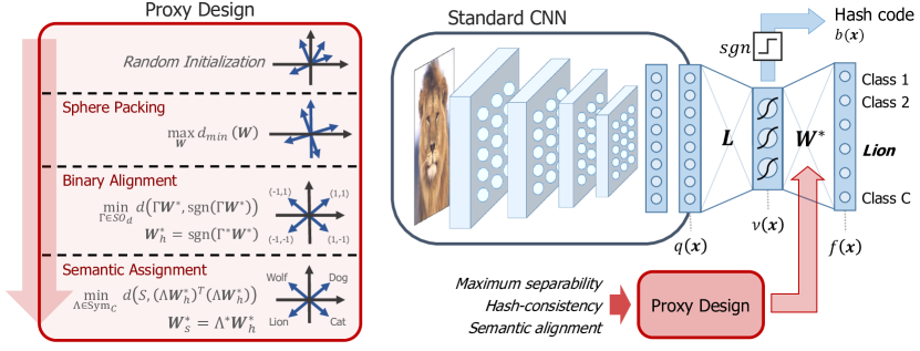
Figure 1: Deep hashing CNN with sHCLM proxies. Left: Proxy design. A set of large margin proxies is first generated by solving a sphere packing problem. A rotation is next applied to render these proxies as binary as possible, and their entries binarized to produce the HCLM proxy set ${\bf W}_{h}^{*}$. Finally, a semantic assignment maps proxies to classes, producing the sHCLM proxy set ${\bf W}_{s}^{*}$ used as weight matrix ${\bf W}^{*}$ of the CNN. Right: Deep hashing CNN. The output of layer $\nu(\mathbf{x})$ is a hashing function, binarized to produce a bit-string $b(\mathbf{x})$ for fast image retrieval.

Early hashing techniques approximated nearest neighbor searches between low-level features Datar:LSH ; Mu:CAI10 ; Gong:ITQ ; Weiss:SH . However, humans judge similarity based on image semantics, such as scenes, objects, and attributes. This inspired the use of semantic representations for image retrieval Lampert:Attributes ; Nikhil:QBSE ; Li:ObjectBank and, by extension, hashing Xia:CNNH ; Lin:BHC ; Zhang:BitScalable ; Zhong:DHN . Modern hashing techniques rely on semantic embeddings implemented with convolutional neural networks (CNNs), as illustrated in Figure 1 (right). A CNN feature extractor $q(\mathbf{x})$ is augmented with a hashing layer that outputs a nearly-binary code $\nu(\mathbf{x})$ using saturating non-linearities, such as a $\operatorname{sigmoid}$ or $\tanh$. The code $\nu(\mathbf{x})$ is thresholded to produce a bitstream $b(\mathbf{x})$, which is the hash code for image $\mathbf{x}$.

The embedding $\nu(\mathbf{x})$ can be learned by metric learning Wang:TripletSH ; Lai:NINH ; liu2016deep or classification Lin:BHC ; Yang:SSDH ; Li:DeepSDH , with classification methods usually being preferred for recognition and metric learning for retrieval. However, it has recently been shown that good retrieval performance can also be achieved with proxy embeddings movshovitz2017 derived from the neighborhood component analysis (NCA) goldberger:NCA metric learning approach. These embeddings learn a set of proxies, or class representatives, around which class examples cluster. Learning involves minimizing a variant of the softmax loss defined by a pre-chosen distance function. For standard distance functions, proxies are identical to the columns ${\bf w}_{y}$ of the weight matrix $\bf W$ of the softmax layer of the classifier of Figure 1. Under such distances, there is little difference between a classifier and a proxy embedding. The architecture of Figure 1 can thus be used both for both classification or retrieval.

Nevertheless, generic embeddings are unsuitable for hashing, where the outputs of $\nu(\mathbf{x})$ should be binary. The goal is to make the $\operatorname{sigmoid}$ or $\tanh$ non-linearities of Figure 1 saturate without degrading classification or retrieval performance. This is difficult because classification and metric learning losses are invariant to rotation. For example, classification losses only depend on the dot-products of $\nu(\mathbf{x})$ and the rows $\mathbf{w}_{y}$ of the matrix $\bf W$. Hence, even if there is a solution $({\bf W},\nu(\mathbf{x}))$ with binary $\nu(\mathbf{x})$, an infinite number of non-binary solutions of equivalent loss can be constructed by rotating both the proxies $\mathbf{w}_{y}$ and the embedding $\nu(\mathbf{x})$. In the absence of further constraints, there is no incentive to learn a binary embedding. Hashing techniques address this by the addition of loss terms that encourage a binary $\nu(\mathbf{x})$ Liong:SDH ; Shen:SDH ; Yang:SSDH ; Lin:UnsHashing ; Cao:DQN . In general, however, this degrades both classification and retrieval performance.

We address this problem by leveraging the observation that the optimally discriminant embedding $\nu(\mathbf{x})$ of image $\mathbf{x}$ must be as aligned as possible (in the dot-product sense) with the proxy $\mathbf{w}_{y}$ of the corresponding class $y$. The rotational ambiguity can thus be removed by using a fixed set of weights $\bf W$ and learning the optimal embedding $\nu(\mathbf{x})$ given these fixed proxies. This allows the encoding in the proxy set $\bf W$ of any properties desired for $\nu(\mathbf{x})$. In this work, we consider the design of proxy sets ${\bf W}^{*}$ that are nearly optimal for both classification and hashing. This involves two complementary goals. On the one hand, classification optimality requires maximum separation between proxies. On the other hand, hashing optimality requires binary proxies.

We show that the first goal is guaranteed by any rotation of the solution of a classical sphere packing optimization problem, known as the Tammes problem Tammes1930 . Drawing inspiration from the classical iterative quantization (ITQ) procedure of Gong:ITQ , we then seek the rotation of the Tammes solution that makes these proxies most binary. This produces a set of hash-consistent large-margin (HCLM) proxies. Unlike ITQ, which rotates the embedding $\nu(\mathbf{x})$, the proposed binary alignment is applied to the proxies only, i.e. before $\nu(\mathbf{x})$ is even learned. The embedding can then be learned end-to-end, guaranteeing that it is optimally discriminant. Also, because this requires $\nu(\mathbf{x})$ to be aligned with the proxies, training $\nu(\mathbf{x})$ for classification also forces its outputs to saturate, eliminating the need for additional binarization constraints. Finally, because the proxies are not learned, learning is freed from rotational ambiguities.

Beyond rotations, the Tammes solution is also invariant to proxy permutations. We leverage this additional degree of freedom to seek the proxy-class assignments that induce a semantically structured $\nu(\mathbf{x})$, where similar proxies represent similar classes. This is denoted the semantic HCLM (sHCLM) proxy set. Since semantically structured embeddings enable more effective transfer to unseen classes Lampert:Attributes ; Akata:ALE ; Morgado:SCoRe , this enhances retrieval performance in transfer scenarios Sablayrolles:SHEval . The steps required for the generation of an sHCLM proxy set are summarized on the left of Figure 1.

Extensive experiments show that sHCLM proxy embeddings achieve state-of-the-art hashing results on several small and large scale datasets, for both classification and retrieval, both within and beyond the set of training classes. We also investigate the combination of proxy and classical triplet embeddings. This shows that their combination is unnecessary for datasets explicitly annotated with classes but can be useful for multi-labeled datasets, where the class structure is only defined implicitly through tag vectors.

2 Related Work

In this section, we review previous work on image embeddings, retrieval, hashing and transfer learning techniques that contextualize our contributions.

Image retrieval:

Content-based image retrieval (CBIR) aims to retrieve images from large databases based on their visual content alone. Early systems relied on similarities between low-level image properties such as color and texture Flickner:QBIC ; bach1996virage ; Smith:VisualSEEk . However, due to the semantic gap between these low-level image representations and those used by humans, such systems had weak performance Smeulders:PAMI00 . This gap motivated substantial research in semantic image embeddings that better align with human judgments of similarity. Early works include query by semantic example Nikhil:QBSE , semantic multinomials pereira2014cross , classeme representations torresani2010efficient , and object banks Li:ObjectBank . These methods used embeddings learned by generative models for images or binary classifiers, usually support vector machines. More recently, CNNs have been used to extract more robust semantic embeddings, with improved retrieval performance gordo2016deep .

Embeddings:

Many algorithms have been proposed to learn embeddings $\nu({\bf x})$ endowed with a metric, usually the Euclidean distance. For this, pairs of examples in a dataset are labeled “similar” or “non-similar,” and a CNN is trained with a loss function based on distances between pairs or triplets of similar and non-similar examples, e.g., the contrastive loss of hadsell2006 (pairs) or the triplet loss of weinberger2009 . These embeddings have been successfully applied to object retrieval bell2015 , face verification sun2014 ; schroff2015 , image retrieval wang2014 , clustering oh2016 , person re-identification zhang2019scan ; zhang2017image among other applications.

Another possibility is to define a class-based embedding. This is rooted in the neighborhood component analysis (NCA) procedure goldberger:NCA , based on a softmax-like function over example distances. However, because NCA requires a normalization over the entire dataset, it can be intractable. Several approximations replace training examples by a set of proxies. sohn2016 proposed the N-tuplet loss, which normalizes over (N+1)-tuplets of examples and wen2016 introduced the center loss, which combines a softmax classifier and an additional term defined by class centers. Finally, movshovitz2017 replaces the $N$-tuplet of examples by a set of learned proxies, or class representatives, around which examples cluster. movshovitz2017 showed that proxy embeddings outperform triplet embeddings schroff2015 ; oh2016 , $N$-tuplet embeddings sohn2016 , and the method of song2 on various retrieval tasks.

Hashing:

Computational efficiency is a major concern for retrieval, since nearest-neighbor search scales poorly with database size. Hashing techniques, based on binary embeddings, enable fast distance computations using Hamming distances. This has made hashing a popular solution for retrieval. Unsurprisingly, the hashing literature experienced a trajectory similar to image retrieval. Early approaches were unsupervised Datar:LSH ; Mu:CAI10 ; Gong:ITQ ; Weiss:SH , approximating nearest-neighbor search in Euclidean space using fast bit operations. Semantic supervision was then introduced to fit the human notion of similarity Wang:SSH ; Kulis:BRE ; Norouzi:MLH ; Liu:KSH . This was initially based on handcrafted features, which limit retrieval performance. More recently, CNNs became dominant. In one of the earliest solutions, PCA and discriminative dimensionality reduction of CNN activations were used to obtain short binary codes Babenko:NeuralCodes . More commonly, the problem is framed as one of joint learning of hash codes and semantic features, with several approaches proposed to achieve this goal, e.g., by exploiting pairwise similarities Xia:CNNH ; Liong:SDH ; Zhu:DHN ; Cao:DQN ; Li:DeepSDH ; jiang2018asymmetric , triplet losses Lai:NINH ; Zhang:BitScalable ; Wang:TripletSH ; Zhang:QaDWH or class supervision Xia:CNNH ; Yang:SSDH ; Lin:BHC ; Zhong:DHN ; Li:DeepSDH ; Zhang:QaDWH .

As shown in Figure 1, most approaches introduce a layer of squashing non-linearities (e.g., $\tanh$ or $\operatorname{sigmoid}$) that, when saturated, produces a binary code. Extensive research has been devoted to the regularization of these networks with losses that favor saturation, using constraints such as maximum entropy Liong:SDH ; Yang:SSDH ; Lin:UnsHashing ; Huang:UTH , independent bits Liong:SDH , low quantization loss Liong:SDH ; Shen:SDH ; Yang:SSDH ; Lin:UnsHashing ; Cao:DQN , rotation invariance Lin:UnsHashing ; Huang:UTH , low-level code consistency Zhang:BitScalable , or bimodal Laplacian quantization priors Zhu:DHN . These constraints compensate for the different goals of classification and hashing, and are critical to the success of most hashing methods. However, they reduce the discriminant power of the CNN. Like these methods, the proposed hashing procedure leverages the robust semantic embeddings produced by CNNs. However, the proposed CNN architecture meets the binarization requirement without the need for binarization losses. We show that, for CNNs with sHCLM proxies, the cross-entropy loss suffices to guarantee binarization.

Transfer protocol for supervised hashing:

Traditional hashing evaluation protocols are class-based. A retrieved image is relevant if it has the same class label as the query or at least one label for multi-labeled datasets. However, a classifier that outputs a single bit per class enables high retrieval performance with extremely small hash codes Sablayrolles:SHEval . The problem is that the traditional protocol ignores the fact that retrieval systems deployed in the wild are frequently confronted with images of classes unseen during training. Ideally, hashing should generalize to such classes. This is unlikely under the traditional protocol, which encourages hash codes that overfit to training classes.

To avoid this problem, Sablayrolles:SHEval proposed to measure retrieval performance on images from previously unseen classes. While some recent works have adopted this protocol Sablayrolles:SHEval ; jain2017subic ; lu2017deep , they still disregard transfer during CNN training. We propose a solution to this problem by explicitly encoding the semantic structure in the sHCLM proxies used for training. Our approach is inspired by the use of semantic spaces for zero-shot and few-shot learning problems Akata:ALE ; Morgado:SCoRe , such as those induced by attributes Lampert:Attributes , large text corpora frome2013devise or other measures of class similarity rohrbach2011evaluating . However, because the goal is to improve hashing performance, proxies need to be optimal for hashing as well. To accomplish this, we propose a procedure to semantically align hash-consistent proxies, with apriori measures of class similarity.

3 Hashing with the Proxy Embedding

Modern hashing algorithms are implemented with CNNs trained for either classification or metric learning. A CNN implements an embedding $\nu:{\cal X}\rightarrow{\cal V}\subset\mathbb{R}^{d}$ that maps image $\mathbf{x}\in{\cal X}$ into a $d$-dimensional feature vector ${\bf v}=\nu(\mathbf{x})$. In this section, we discuss the limitations of current embeddings for hashing.

3.1 Classification vs. Metric Learning

For classification, image $\mathbf{x}$ belongs to a class drawn from random variable $Y\in\{1,\ldots,C\}$. Given a dataset ${\cal D}=\{(\mathbf{x}_{i},y_{i})\}_{i=1}^{n}$, a CNN is trained to discriminate the $C$ classes by minimizing the empirical cross-entropy loss

$${\cal R}=-\sum_{i}\log P_{Y|\mathbf{X}}(y_{i}|\mathbf{x}_{i}),$$ (1)

where $P_{Y|\mathbf{X}}(y|\mathbf{x})$ are posterior class probabilities modeled by softmax regression

$$P_{Y|\mathbf{X}}(y|\mathbf{x})=\frac{e^{\mathbf{w}_{y}^{T}\nu(\mathbf{x})+b_{y}}}{\sum_{k}e^{\mathbf{w}_{k}^{T}\nu(\mathbf{x})+b_{k}}},$$ (2)

where $\mathbf{w}_{y}$ is the parameter vector for class $y$ and $b_{y}$ the class bias.

For metric learning, the goal is to endow the feature space $\cal V$ with a metric, usually the squared Euclidean distance, to allow operations like retrieval. Although seemingly different, metric learning and classification are closely related. As shown in Appendix A, learning the embedding $\nu(\mathbf{x})$ with (1) using the softmax classifier of (2) is equivalent to using

$$P_{Y|\mathbf{X}}(y|\mathbf{x})=\frac{e^{-d_{\phi}(\nu(\mathbf{x}),\mu_{y})}}{\sum_{k}e^{-d_{\phi}(\nu(\mathbf{x}),\mu_{k})}},$$ (3)

where $d_{\phi}$ is a Bregman divergence bregman1967 and $\mu_{y}$ the mean of class $y$. Hence, any classifier endows the embedding $\nu(\mathbf{x})$ with a metric $d_{\phi}$. This metric is the Euclidean distance if and only if

$$P_{Y|\mathbf{X}}(y|\mathbf{x})=\frac{e^{-d_{\phi}(\nu(\mathbf{x}),\mathbf{w}_{y})}}{\sum_{k}e^{-d_{\phi}(\nu(\mathbf{x}),\mathbf{w}_{k})}},$$ (4)

in which case (4) is identical to (2). In sum, training an embedding with the Euclidean distance is fundamentally not very different from training the softmax classifier.

In fact, the combination of (1) and (4) is nearly identical to the proxy embedding technique of movshovitz2017 . This is a metric learning approach derived from neighborhood component analysis (NCA) goldberger:NCA , which denotes the parameters $\mathbf{w}_{y}$ as a set of proxy vectors. The only difference is that, in NCA, the probabilities of (4) are not properly normalized, since the summation in the denominator is taken over $k\neq y$. However, because there are usually many terms in the summation, the practical difference is small. Therefore, we refer to an embedding $\nu(\mathbf{x})$ learned by cross-entropy minimization with either the model of (2) or (4) as the proxy embedding. This is a unified procedure for classification and metric learning, where the parameters $\mathbf{w}_{y}$ can be interpreted as either classifier parameters or metric learning proxies.

3.2 Deep Hashing

Given an embedding $\nu(\mathbf{x})$ endowed with a metric $d(\cdot,\cdot)$, image retrieval can be implemented by a nearest-neighbor rule. The query $\bf x$ and database images ${\bf z}_{i}$ are forward through the CNN to obtain the respective vector representations $\nu(\mathbf{x})$ and $\nu({\bf z}_{i})$, and database vectors $\nu({\bf z}_{i})$ are ranked by their similarity to the query $\nu(\mathbf{x})$. This requires floating point arithmetic for the metric $d(\cdot,\cdot)$ and floating point storage for the database representations $\nu({\bf z}_{i})$, which can be expensive. Hashing aims to replace $\nu(\mathbf{x})$ with a bit-string $b(\mathbf{x})$, known as the hash code, and $d(\cdot,\cdot)$ with a low complexity metric, such as the Hamming distance

$$d(\mathbf{x},{\bf z}_{i})=\sum_{c}b_{c}(\mathbf{x})\oplus b_{c}({\bf z}_{i})$$ (5)

where $\oplus$ is the XOR operator.

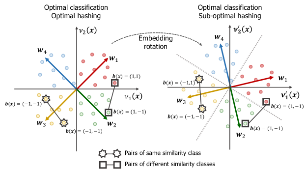
Figure 2: Effects of rotation on optimality for classification and hashing. The figure depicts two possible embeddings for classification or hashing. Because the two solutions differ by a joint rotation of feature vectors $\nu(\mathbf{x})$ and proxies $\mathbf{w}_{y}$, and the loss of (8) only depends on the dot-products $\langle\nu(\mathbf{x}),\mathbf{w}_{y}\rangle$, the two solutions are equally optimal for classification. This is, however, not the case for hashing. While, on the left, binarization maps all the examples from the same class into the same hash code $b(\mathbf{x})$, this is not true on the right. Best viewed in color.

In the hashing literature, the proxy embedding is frequently used to obtain hash codes. Figure 1 (right) illustrates the architecture commonly used to produce $b(\mathbf{x})$. A CNN encoder first extracts a feature representation $q(\mathbf{x})$ from image $\bf x$. This is then mapped into the low-dimensional embedding $\nu(\mathbf{x})\in\mathbb{R}^{d}$. A $d$-bit hash code is finally generated by thresholding $\nu(\mathbf{x})$

$$b(\mathbf{x})=\operatorname{sgn}(\nu(\mathbf{x})),$$ (6)

where $\operatorname{sgn}(\cdot)$ is the vector of signs of its entries. This network is trained for either classification or metric learning, using a softmax regression layer of the form of (2) or (4), respectively. The network parameters are trained to optimize (1).

For hashing, the binarization error of (6) must be as small as possible. This is encouraged by implementing the mapping $q(\mathbf{x})\to\nu(\mathbf{x})$ as

$$\nu(\mathbf{x})=\tanh({\bf L}^{T}q(\mathbf{x})+{\bf b})\in\mathbb{R}^{d},$$ (7)

where $\bf L$ is a dimensionality reduction matrix, ${\bf b}$ a bias vector and $\tanh(\cdot)$ an element-wise squashing non-linearity. The introduction of these non-linearities encourages $\nu(\mathbf{x})$ to be binary by saturation, i.e. by making the output of $\tanh(\cdot)$ close to its asymptotic values of $+1$ or $-1$. Under this assumption, $b(\mathbf{x})\approx\nu(\mathbf{x})$ and there is no information loss due to the binarization of (6). Since the cross-entropy risk encourages $\nu(\mathbf{x})$ to maximally discriminate similarity classes, the same holds for the hash codes $b(\mathbf{x})$. These properties have made the architecture of Figure 1 popular for hashing Xia:CNNH ; Yang:SSDH ; Lin:BHC ; Zhong:DHN ; Li:DeepSDH ; Zhang:QaDWH .

3.3 Challenges

The discussion above assumes that it is possible to obtain a discriminative embedding $\nu(\mathbf{x})$ with saturated non-linearities, by training the CNN of Figure 1 for classification or metric learning. However, this problem does not have a unique solution. Even when it is optimal for $\nu(\mathbf{x})$ to saturate, many equivalent solutions do not exhibit this behavior. This has been experimentally observed by previous works, which proposed learning the CNN with regularization losses that penalize large binarization errors Liong:SDH ; Shen:SDH ; Yang:SSDH ; Lin:UnsHashing ; Cao:DQN . In our experience, these approaches fail to guarantee both optimal classification and saturation of hash scores. Instead, there is usually a trade-off, where emphasizing one component of the loss weakens performance with respect to the other.

This can be understood by writing the cross-entropy as

$$L_{p}(\mathbf{x},y)=-\log\frac{e^{\langle\nu(\mathbf{x}),\mathbf{w}_{y}\rangle}}{\sum_{k}e^{\langle\nu(\mathbf{x}),\mathbf{w}_{k}\rangle}}.$$ (8)

Since (8) is minimum when $\left<\nu(\mathbf{x}),\mathbf{w}_{y}\right>$ is much larger than all other $\left<\nu(\mathbf{x}),\mathbf{w}_{k}\right>$, cross-entropy minimization encourages the embedding to align with the proxy of the ground-truth class $y$

$$\nu^{*}(\mathbf{x})\propto\mathbf{w}_{y}.$$ (9)

This is illustrated in Figure 2 for a classifier with $C=4$ classes, proxies $\mathbf{w}_{c}$ and embedding $\nu(\mathbf{x})$ of dimension $d=2$. The embeddings $\nu(\mathbf{x})$ of each similarity class (points of a given color) cluster around the corresponding proxy (vector of the same color). However, this solution is not unique. Since all dot-products of (8) are unchanged by a joint rotation of $\nu(\mathbf{x})$ and $\mathbf{w}_{c}$, the cross-entropy loss is invariant to rotations. In Figure 2, a rotation transforms the boundaries between classes from the coordinate axes on the left to the dashed lines on the right. From a classification perspective, the two solutions are identical.

For hashing, however, the two solutions are different. On the left, where each class occupies its own quadrant, all examples from the same similarity class share the same hash code $b(\mathbf{x})$ (as defined in (6)), while distinct hashes identify examples from different classes. This makes the hash codes optimal for retrieval. However, on the right, examples marked by a square have zero Hamming distance, despite belonging to different classes, and those marked by a star have distance one, despite belonging to the same class. In summary, while the two solutions are optimal for classification, only the one on the left is optimal for hashing. Thus, when the network of Figure 1 is trained to optimize classification, the introduction of the $\tanh$ non-linearities in (7) is not enough to guarantee good hash codes. Once the learning algorithm reaches the solution on the right of Figure 2, there is no classification benefit to pursuing that on the left. Since there is an infinite number of rotations that produce equally optimal solutions for classification, it is unlikely that the algorithm will ever produce the one optimal for hashing.

4 Learning Proxies for Hashing

In this section, we introduce a procedure to design proxies that induce good hashing performance.

4.1 Joint Optimality for Classification and Hashing

So far we have seen that, because cross-entropy optimization leads to (9), the set of proxies ultimately defines the properties of the learned embedding. This suggests that, rather than learning both embedding and proxies simultaneously, learning can proceed in two steps:

1. Design a set of proxies $\mathbf{w}^{*}_{y}$ that encourages an embedding $\nu(\mathbf{x})$ optimal for classification and hashing;

2. Learn the embedding $\nu^{*}(\mathbf{x})$ by optimizing the CNN with the cross-entropy loss, while keeping the proxies $\mathbf{w}^{*}_{y}$ fixed.

The ensuing question is “which properties the set of proxies $\mathbf{w}_{y}$ must have to encourage optimal classification and hashing?”

Proxies for optimal classification:

To determine how the set of proxies can encourage optimal classification, we note that models learned by cross-entropy minimization are (approximately) max-margin classifiers. This can be seen by writing (8) as

$$\textstyle L_{p}(\mathbf{x},y)=\log\left[1+\sum_{c\neq y}e^{\langle\nu(\mathbf{x}),\mathbf{w}_{c}\rangle-\langle\nu(\mathbf{x}),\mathbf{w}_{y}\rangle}\right].$$ (10)

Due to the exponent, the sum is dominated by the largest term, and minimizing (10) is equivalent to minimizing $\max_{c\neq y}\langle\nu(\mathbf{x}),\mathbf{w}_{c}\rangle-\langle\nu(\mathbf{x}),\mathbf{w}_{y}\rangle$. Hence, the network seeks a predictor that maximizes the classification margin

$${\cal M}(\nu(\mathbf{x}),y) =\langle\nu(\mathbf{x}),\mathbf{w}_{y}\rangle-\max_{c\neq k}\langle\nu(\mathbf{x}),\mathbf{w}_{c}\rangle.$$ (11)

For the predictor of (9), this is given by

$${\cal M}(\nu^{*}(\mathbf{x}),y) \propto||\mathbf{w}_{y}||^{2}-\max_{c\neq k}\langle\mathbf{w}_{y},\mathbf{w}_{c}\rangle.$$ (12)

Hence, to encourage classification optimality, it suffices to chose a set of fixed norm proxies, $||\mathbf{w}_{c}||^{2}=K,c=\{1,\ldots,C\}$, that maximizes

$$\textstyle{\cal M}_{y}=K-\max_{c\neq y}\left<\mathbf{w}_{y},\mathbf{w}_{c}\right>,$$ (13)

for all $y$, simultaneously. This is equivalent to solving

$$\mathbf{W}^{*}= \underset{\mathbf{w}_{1},\ldots,\mathbf{w}_{C}}{\arg\max} \min_{i\neq j}||\mathbf{w}_{i}-\mathbf{w}_{j}||^{2}$$ (14)

subject to $$||\mathbf{w}_{c}||^{2}=K\quad\forall c,$$

a classical problem in mathematics, known as the Tammes or sphere packing problem Tammes1930 , when $K=1$. The Tammes problem determines the maximum diameter of $C$ equal circles that can be placed on the surface of the unit sphere without overlap. In sum, a network trained to minimize classification loss encourages predictions aligned with proxies $\mathbf{w}_{y}$ for images of class $y$. Thus, classification margins are maximized when the proxy set is maximally separated, i.e., when the proxies are given by the Tammes solution $\mathbf{W}^{*}$.

Hashing optimal proxies:

Since embeddings $\nu^{*}(\mathbf{x})$ cluster around the proxies of the corresponding class $\mathbf{w}_{y}$, binary proxies encourage binary embedding representations. Note that this is what is special about the solution of Figure 2 (left). Thus, joint optimality for classification and hashing is guaranteed by any set of binary proxies that solve (14), i.e.

$$\mathbf{W}_{h}^{*}= \underset{\mathbf{w}_{1},\ldots,\mathbf{w}_{C}}{\arg\max} \min_{i\neq j}||\mathbf{w}_{i}-\mathbf{w}_{j}||^{2}$$ (15)

subject to $$\mathbf{w}_{c}\in\{-1,1\}^{d}\quad\forall c.$$

Since learning the CNN with proxies $\mathbf{W}_{h}^{*}$ as a fixed set of weights on the final softmax regression layer already encourages a binary $\nu^{*}(\mathbf{x})$, the CNN can be trained to optimize classification only. The binarization step incurs no loss of classification performance and there is no need to define additional cost terms, which often conflict with classification optimality. Finally, CNN optimization no longer has to deal with the ambiguity of multiple solutions optimal for classification but not hashing.

4.2 Proxy design

It remains to determine a procedure to design the proxy set. This is not trivial, since (15) is a discrete optimization problem. In this work, we adopt an approximate solution composed of two steps. First, we solve the Tammes problem of (14) using a barrier method Wright:Optimization to obtain $\mathbf{W}^{*}$, which we denote the Tammes proxies. Since the problem is convex, this optimization is guaranteed to produce a maximally separated proxy set. However, since any rotation around the origin leaves the norms of (14) unchanged, Tammes proxies are only defined up to a rotation. We exploit this degree of freedom to seek the rotation $\mathbf{\Gamma}^{*}$ that makes the Tammes proxies most binary. This consists of solving

$$\mathbf{\Gamma}^{*} = \arg\min_{\mathbf{\Gamma}\in SO_{d}}\textstyle\sum_{k}\|\mathbf{\Gamma}\mathbf{w}_{k}^{*}-\operatorname{sgn}(\mathbf{\Gamma}\mathbf{w}_{k}^{*})\|^{2}$$ (16)

and is an instance of the binary quantization problem studied in Gong:ITQ . Given $\mathbf{W}^{*}$, we use the ITQ binary quantization algorithm of Gong:ITQ to find the optimal rotation $\mathbf{\Gamma}^{*}$ of (16). It should be emphasized that, unlike previous uses of ITQ, the procedure is not used to binarize $\nu(\mathbf{x})$, but to generate proxies that induce a binary $\nu(\mathbf{x})$. This enables end-to-end training under a classification loss that seeks maximum discrimination between the classes used to define image similarity. Finally, the proxy matrix

$$\mathbf{W}^{*}_{h}=\operatorname{sgn}(\mathbf{\Gamma}^{*}\mathbf{W}^{*}).$$ (17)

is used to determine the weights of the softmax regression layer. We denote $\mathbf{W}^{*}_{h}$ as the hash-consistent large margin (HCLM) proxy set.

4.3 Class/proxy matching

HCLM proxies $\mathbf{w}_{y}$ induce hash codes with good properties for both classification and retrieval. However because $\mathbf{w}_{y}$ are simply a set of multi-dimensional class labels, any permutation of the indices $y$ produces a set of valid proxies. This is probably best understood by referring to the four class example of Figure 2. Assume that, in this example, the classes were “A: apples,” “C: cats,” “D: dogs,” and “O: oranges.” While HCML generates the set of vectors $\mathbf{w}_{y}$, it does not determine which vector in ${\cal W}=\{\mathbf{w}_{1},\mathbf{w}_{2},\mathbf{w}_{3},\mathbf{w}_{4}\}$ should be paired with each label in ${\cal L}=\{A,C,D,O\}$.

While, in principle, with enough data and computation, the embedding model $\nu(\cdot)$ could be trained to map images $\mathbf{x}$ into the geometry induced by any pairing between the elements of $\cal W$ and $\cal L$, some pairings are easier to learn than others. Because learning is initialized with the feature extractor $q(\mathbf{x})$ from the pre-trained network (see Figure 1), the embedding $\nu(\cdot)$ should be easier to learn when the pairing of proxies and classes respects the similarity structure already available in this feature space. In the example above, classes C and D will induce feature vectors in $q(\mathbf{x})$ that are more similar than those of either the pair (C,A) or (D,A). Similarly, the features vectors of classes A and O will be closer to each other than to those of the other classes.

It follows that the pairing {($\mathbf{w}_{1}$, A), ($\mathbf{w}_{2}$,O), ($\mathbf{w}_{3}$, C), ($\mathbf{w}_{4}$, D)}, where the vectors of similar classes are close to each other, respects the structure of the feature space much better than the pairing {($\mathbf{w}_{1}$, A), ($\mathbf{w}_{2}$,C), ($\mathbf{w}_{3}$, O), ($\mathbf{w}_{4},D)\}$, where they are opposite to each other. More generaly, if classes $i$ and $j$ induce similar feature vectors in $q(\mathbf{x})$, which are both distant from the feature vectors induced by class $z$, the assignment of proxies to classes should guarantee that $d(\mathbf{w}_{i},\mathbf{w}_{j})$ is smaller than $d(\mathbf{w}_{i},\mathbf{w}_{z})$ and $d(\mathbf{w}_{j},\mathbf{w}_{z})$. This avoids the model $q(\mathbf{x})$ to be required to relearn the structure of the metric space, making training more data efficient, and ultimately leading to a better hashing system.

Hence, the goal is to align the proxy similarities $\mathbf{w}_{y_{i}}^{T}\mathbf{w}_{y_{j}}$ with some measure of similarity $s_{ij}$ between feature vectors $q(\mathbf{x})$ from classes $i$ and $j$. This can be done by searching for the proxy assignments $\gamma_{1},\ldots,\gamma_{C}$ that minimize

$$\textstyle\min_{\gamma_{1},\ldots,\gamma_{C}}\quad\sum_{i\neq j}s_{ij}(1-\mathbf{w}_{\gamma_{i}}^{T}\mathbf{w}_{\gamma_{j}}^{T}).$$ (18)

Although this is a combinatorial optimization problem, in our experience, a simple greedy optimization is sufficient to produce a good solution. Starting from a random class assignment, the proxy swap that leads to the greatest decrease in (18) is taken at each iteration, until no further improvement is achieved. This alignment procedure is applied to HCLM to produce a semantic HCLM (sHCLM) proxy set. It remains to derive a procedure to measure the similarities $s_{ij}$ between classes. We consider separately the cases where image similarity is derived from single and multi labeled data.

Single label similarity: For single labeled data, we first compute the average code ${\bf u}_{y}$ of class $y$, by averaging the feature vectors $q(\mathbf{x}_{i})$ produced by the pre-trained network for training images $\mathbf{x}_{i}$ of class $y$

$${\bf u}_{y}=\frac{1}{n}\sum_{\mathbf{x}_{i}:y_{i}=y}q(\mathbf{x}_{i}).$$ (19)

Pairwise similarities between training classes $y_{i}$ and $y_{j}$ are then computed with

$$\textstyle s_{ij}=\exp\left\{-\frac{\|{\bf u}_{y_{i}}-{\bf u}_{y_{j}}\|^{2}}{2\kappa^{2}}\right\},$$ (20)

where $\kappa$ is the average distance between means ${\bf u}_{i}$. This procedure can also be justified by the fact that, as shown in Appendix A  (38) and (40), when $d(\cdot,\cdot)$ is the $L_{2}$ distance, the proxy $\mathbf{w}_{y}$ is the average $\mu_{y}^{\nu}$ of the feature vectors $\nu(\mathbf{x}_{i})$ extracted from class $y$. However, because the class-proxy assignments must be defined before training the network, the embedding $\nu(\mathbf{x})$ is not available. The use of (19) corresponds to approximating the distance between vectors $\nu(\mathbf{x})$ by the distance between the vectors $q(\mathbf{x})$ computable with the pre-trained network. Note that slightly better performance could likely be attained by first fine-tuning the pre-trained network on the target dataset, without layers ${\bf L}$ and ${\bf W}^{*}$ of Figure 1. However, this would increase training complexity and is not used in this work.

Multi label similarity: In multi labeled datasets, images are not described by a single class. Instead, each image is annotated with $T$ auxiliary semantics (or tags) that indicate the presence/absence of $T$ binary visual concepts. Each image $\mathbf{x}$ is labeled with a binary vector $\bf t$, such that $t_{k}=1$ if the $k^{th}$ tag is associated with the image and $t_{k}=0$ otherwise. In this case, proxies ${\bf w}_{i}$ are assigned to each tag $t_{i}$.

Given a multi-labeled dataset, (19) and (20) could be used to compute tag similarities. However, we found experimentally that using tag co-occurrence as a measure of similarity can also yield strong performance. Specifically, the similarity $s_{ij}$ between tags $t_{i}$ and $t_{j}$ was computed as

$$s_{ij}=\frac{2\sum_{n}t_{n,i}\;t_{n,j}}{\sum_{n}t_{n,i}+\sum_{n}t_{n,j}},$$ (21)

where $t_{n,i}\in\{0,1\}$ denotes the $i^{th}$ tag of sample ${\bf x}_{n}$. The similarity $s_{ij}$ approaches one when the $i^{th}$ and $j^{th}$ tags co-occur with high chance and is close to zero when the two tags never appear together. This procedure has two advantages. First, it encourages tags that often co-occur to have similar proxies (i.e. to share bits of the hash code). Second, it has smaller complexity, since there is no need to forward images through the network to compute (19).

4.4 Joint Proxy and Triplet Embedding

So far, we have considered metric learning with proxy embeddings. An alternative approach is to abandon the softmax regression of (2) and apply a loss function directly to $\nu(\mathbf{x})$. While many losses have been proposed chopra2005 ; hadsell2006 ; sohn2016 ; oh2016 , the most popular operate on example triplets, pulling together (pushing apart) similar (dissimilar) examples weinberger2009 ; wang2014 ; bell2015 ; schroff2015 . These methods are commonly known as triplet embeddings. When compared to proxy embeddings, they have both advantages and shortcomings. On one hand, because the number of triplets in the training set is usually very large, a subset of triplets must be sampled for learning. Despite the availability of many sampling strategies schroff2015 ; wang2014 ; oh2016 ; sun2014 , it is usually impossible to guarantee that the similarity information of the dataset is fully captured. Furthermore, because they do not directly leverage class labels, triplet embeddings tend to have weaker performance for classification. On the other hand, because the similarity supervision is spread throughout the feature space, rather than concentrated along class proxies, they tend to better capture the metric structure of the former away from the proxies. This more uniform learning of metric structure is advantageous for applications such as retrieval or transfer learning, where triplet embeddings can outperform proxy embeddings.

In this work, we found that combining proxy and triplet embeddings is often advantageous. Given an anchor ${\bf x}$, a similar ${\bf x}^{+}$ and a dissimilar example ${\bf x}^{-}$, we define the triplet loss in Hamming space by the logistic loss with a margin of $m$ bits

$$L_{t}(\mathbf{x},\mathbf{x}^{+},\mathbf{x}^{-})=\log\left(1+e^{m+d_{H}(\mathbf{x},\mathbf{x}_{p})-d_{H}(\mathbf{x},\mathbf{x}_{n})}\right).$$ (22)

Since, in hashing, $\nu(\mathbf{x})\in[-1,1]$ represents a continuous surrogate of the hash codes $b(\mathbf{x})\in\{0,1\}$, Hamming distances between two images $\mathbf{x}_{i}$ and $\mathbf{x}_{j}$ are estimated with the distance function

$$d_{H}(\mathbf{x}_{i},\mathbf{x}_{j})=\frac{1}{2}\left(b-\nu(\mathbf{x}_{i})^{T}\nu(\mathbf{x}_{j})\right).$$ (23)

Finally, given an sHCLM proxy set $\{\mathbf{w}_{y}\}_{y=1}^{C}$ of $C$ classes, the embedding is learned by 1) fixing the weights of the softmax regression layer to the proxies $\mathbf{w}_{y}$, and 2) learning the embedding $\nu(\mathbf{x})$ to minimize

$$L({\bf x},y,{\bf x}^{+},{\bf x}^{-})=L_{p}({\bf x},y)+\lambda L_{t}({\bf x},{\bf x}^{+},{\bf x}^{-})$$ (24)

where $L_{p}$ is the proxy loss, $L_{t}$ given by (22) and $\lambda$ is an hyper-parameter that controls their trade-off. In preliminary experiments, we found that the performance of joint embeddings is fairly insensitive to the value of $\lambda$. Unless otherwise noted, we use $\lambda=1$ in all our experiments. The proxy loss $L_{p}({\bf x},y)$ is defined as the softmax cross-entropy loss (1) in the case of single label similarities. For multi label similarities, to account for the fact that tag frequencies are often imbalanced, we adopt a balanced binary cross-entropy xie2015holistically

$$\textstyle L_{p}({\bf x},{\bf t}) =-\textstyle\sum_{k} c_{k}t_{k}\log s_{k}({\bf x})+$$

$$(1-c_{k})(1-t_{k})\log(1-s_{k}({\bf x}))$$

where $s_{k}({\bf x})=\frac{1}{1+e^{{\bf w}_{k}^{T}\nu({\bf x})}}$ and $c_{k}$ is the inverse of the frequency of the $k^{th}$ tag .

5 Experiments

In this section, we present an extensive experimental evaluation of the proposed hashing algorithm.

5.1 Experimental setup

A training set is used to learn the CNN embedding $\nu(\mathbf{x})$, a set of images is defined as the image database and another set of images as the query database. Upon training, the goal is to rank database images by their similarity to each query.

Datasets

Experiments are performed on four datasets. CIFAR-10 CIFAR and CIFAR-100 CIFAR consist of 60 000 color images (32$\times$32) from 10 and 100 image classes, respectively. Following the typical evaluation protocol Wang:TripletSH ; he2018hashing ; Li:DeepSDH ; Xia:CNNH , we use the CIFAR test sets to create queries and the training sets for both training and retrieval databases. NUS-WIDE NUS-WIDE is a multi-label dataset composed of 270 000 web images, annotated with multiple labels from a dictionary of 81 tags. Following standard practices for this dataset Wang:TripletSH ; Li:DPSH ; Zhang:BitScalable ; Li:DeepSDH , we only consider images annotated with the 21 most frequent tags. 100 images are sampled per tag to construct the query set, and all remaining images are used both for training and as the retrieval database. ILSVRC-2012 Deng:Imagenet is a subset of ImageNet with more than 1.2 million images of 1 000 classes. In this case, the standard validation set (50 000 images) is used to create queries, and the training set for learning and retrieval database.

Image representation

Unless otherwise specified, the base CNN of Figure 1 is AlexNet Krizhevsky:Alexnet pre-trained on the ILSVRC 2012 training set and finetuned to the target dataset. Feature representations $q(\mathbf{x})$ are the 4096-dimensional vectors extracted from the last fully connected layer before softmax regression (layer fc7). On the CIFAR datasets, images are resized from the original 32$\times$32 into 227$\times$227 pixels, and random horizontal flipping is applied during training. On ILSVRC-2012 and NUS-Wide, images are first resized to 256$\times$256, and in addition to horizontal flipping, random crops are used for data augmentation. The central 227$\times$227 crop is used for testing.

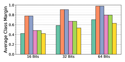
(a) Classification margins.

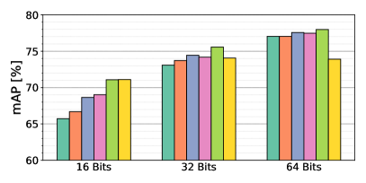
(b) Retrieval performance (mAP).

Figure 3: Classification and retrieval performance using different types of proxies on CIFAR-100.

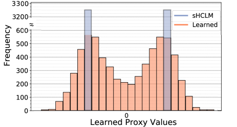
(a) Histogram of Learned and sHCLM proxy weights.

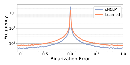
(b) Histogram of binarization errors.

Figure 4: Analysis of 64-bit proxy sets for hashing on CIFAR-100.

Baselines

Various methods from the literature were used for comparison, 1) classical (shallow) unsupervised algorithms, LSH Datar:LSH and ITQ Gong:ITQ ; 2) classical (shallow) supervised algorithms: SDH Shen:SDH , KSH Liu:KSH and ITQ with Canonical Correlation Analysis (ITQ-CCA) Gong:ITQ ; and 3) deep supervised hashing algorithms: DQN Cao:DQN , CNNH Xia:CNNH , NINH Lai:NINH , DSRH Zhao:DSRH , DRSCH Zhang:BitScalable , SSDH Yang:SSDH , DPSH Li:DPSH , SUBIC jain2017subic , BHC Lin:BHC , DTSH Wang:TripletSH , MI-Hash Cakir:MIHash , TALR-AP he2018hashing , DSDH Li:DeepSDH , HBMP cakir2018hashing either based on weighted Hamming distances (denoted “HBMP regress” in cakir2018hashing ) or binary Hamming distances (denoted “HBMP constant” in cakir2018hashing ), and ADSH jiang2018asymmetric . We restate published results when available. Author implementations with default parameters were used for LSH, ITQ, ITQ-CCA, SDH, and KSH with off-the-shelf AlexNet features. We also report results for BHC, SSDH and DTSH for experimental settings not considered in the original paper. To ensure representative performances, we first reproduced published results, typically on CIFAR-10, using author implementations, and then apply the same procedure to the target dataset.

Evaluation metrics

Retrieval performance is evaluated using the mean of the average precision (mAP) across queries. Given a ranked list of $n$ database matches to a query image $\mathbf{x}$, the aggregate precision of the top-$k$ results, over all cutoffs $k$, is computed with

$$AP=\sum_{k=1}^{n}P(k)\Delta r(k)$$ (26)

where $P(k)$ is the precision at cutoff $k$, and $\Delta r(k)$ the change in recall from matches $k-1$ to $k$. For both NUS-WIDE and ImageNet, only the top $n=50\,000$ retrievals are considered when computing the AP. For CIFAR-10 and CIFAR-100, AP is computed over the full ranking. The mAP is the average AP value over the set of queries.

5.2 Learning to hash with explicit class similarities

We start by evaluating hashing performance on datasets where image similarity is directly derived from class labels (CIFAR-10, CIFAR-100, and ISLVRC-2012).

5.2.1 Ablation study

We start by ablating the proxy generation procedure of Figure 1, using the CIFAR-100 dataset. Several embeddings were trained on this dataset, each using a different proxy version. The proxies are as follows.

1. Learned: proxy set learned by back-propagation;

2. Random: fixed random proxies;

3. Tammes: optimal solution $\mathbf{W}^{*}$ to the Tammes problem of (14);

4. Aligned: proxy set $\mathbf{\Gamma}^{*}\mathbf{W}^{*}$ obtained by rotating $\mathbf{W}^{*}$ with the rotation matrix $\mathbf{\Gamma}^{*}$ of (16);

5. HCLM: HCLM proxy set $\mathbf{W}_{h}^{*}$ of (17) (with random proxy/class assignments);

6. sHCLM: HCLM set after the semantic proxy/class assignment of (18).

Figure 3a shows the margin associated with each proxy set (computed with (13)) averaged across classes. Figure 3b compares the retrieval performance of the resulting hash codes. These results support several conclusions. First, as expected, Tammes produces the largest classification margins. However, because it disregards the binarization requirements of hashing, it induces an embedding of relatively weak retrieval performance. This can also be seen by the retrieval gains of Aligned over Tammes. Since the two proxy sets differ only by a rotation, they have equal classification margins. However, due to (9), “more binary” proxies force more saturated responses of the $\tanh(\cdot)$ non-linearities and smaller binarization error. This improves the retrieval performance of the embedding. Second, while the binarization step of (17) reduces classification margins, it does not affect retrieval performance. In fact, the HCLM embedding has better retrieval performance than the Aligned embedding for hash codes of small length. Third, the mAP gains of sHCLM over HCLM show that explicitly inducing a semantic embedding, which maps semantically related images to similar hash codes, further improves retrieval performance. Overall, the sHCLM embedding has the best retrieval performance. Finally, the Learned embedding significantly underperforms the sHCLM embedding. This shows that, at least for hashing, proxy embeddings cannot be effectively learned by back-propagation. In fact, for large code lengths, Learned proxies underperformed Random proxies in terms of both class margins and retrieval performance. As discussed in Sec. 3.3, this is explained by the fact that the cross-entropy loss is invariant to proxy rotations and most rotations do not induce low binarization error. This compromises the effectiveness of proxies learned by back-propagation for the hashing scenario.

To better quantify this issue, we compared the sHCLM and Learned proxy sets in more detail for hash codes of 64 bits. Figure 4a shows the histogram of weight values for the learned and sHCLM proxies. It is clear that, even when the proxy set is learned, the weights are bimodal. This is due to the inclusion of the $\tanh(\cdot)$ non-linearities at the output of $\nu(\mathbf{x})$ and (9). However, unlike the sHCLM proxy sets (which are binary by construction), the weight distribution exhibits significant dispersion around the two modes. Since learned proxies are less binary than sHCLM, the same holds for the embedding $\nu(\mathbf{x})$. This is confirmed by the binarization error histograms of Figure 4b, which show a more binary embedding for sHCLM. In result, even though the sHCLM and Learned embeddings have nearly equal classification accuracy on CIFAR-100 (75.5% and 75.4%, respectively), sHCLM substantially outperforms the Learned proxy set for retrieval (Figure 3b).

Table 1: Retrieval performance (mAP) under supervised protocol on CIFAR-10. ^∗ Self-implementation

	Hash size
	16 Bits	24 Bits	32 Bits	48 Bits
Classical
LSH Datar:LSH	17.5	20.2	20.4	21.2
ITQ Gong:ITQ	22.9	24.3	24.8	25.6
KSH Liu:KSH	47.8	50.5	50.4	52.8
SDH Shen:SDH	66.5	68.3	70.0	71.3
ITQ-CCA Gong:ITQ	71.4	72.6	74.1	74.8
Proxy embeddings
SUBIC jain2017subic	63.5	67.2	68.2	68.6
BHC* Lin:BHC	93.3	93.6	94.0	94.0
SSDH* Yang:SSDH	93.6	93.9	94.2	94.1
Pair-wise embeddings
DQN Cao:DQN	—	55.8	56.4	58.0
DPSH Li:DPSH	76.3	78.1	79.5	80.7
HBMP cakir2018hashing	94.2	94.4	94.5	94.6
ADSH jiang2018asymmetric	89.0	92.8	93.1	93.9
Triplet embeddings
NINH Lai:NINH	—	56.6	55.8	58.1
DRSCH Zhang:BitScalable	61.5	62.2	62.9	63.1
DTSH Wang:TripletSH	91.5	92.3	92.5	92.6
Ranking embeddings
DSRH Zhao:DSRH	60.8	61.1	61.7	61.8
MI-Hash Cakir:MIHash	92.9	93.3	93.8	94.2
TALR-AP he2018hashing	93.9	94.1	94.3	94.5
Combinations
CNNH Xia:CNNH	55.2	56.6	55.8	58.1
DSDH Li:DeepSDH	93.5	94.0	93.9	93.9
Proposed
sHCLM	94.5	94.7	95.2	94.9
sHCLM + Triplet	94.5	94.7	94.9	95.0

5.2.2 Comparison to previous work

We compared the hashing performance of various embeddings on CIFAR-10, CIFAR-100 and ImageNet.

CIFAR-10:

Since CIFAR-10 is one of the most popular benchmarks for hashing, it enables a more extensive comparison. Table 1 restates the performance of various methods as reported in the original papers, when available. The exceptions are classical hashing algorithms, namely LSH Datar:LSH , ITQ Gong:ITQ , SDH Shen:SDH , KSH Liu:KSH and ITQ with Canonical Correlation Analysis (ITQ-CCA) Gong:ITQ . In these cases, we used author implementations with default parameters and off-the-shelf AlexNet fc7 features as input image representations. We also compare to several representatives of the deep hashing literature, including triplet embeddings (NINH Lai:NINH , DRSCH Zhang:BitScalable and DTSH Wang:TripletSH ), pairwise embeddings (DQN Cao:DQN , DPSH Li:DPSH , HBMP cakir2018hashing , and ADSH jiang2018asymmetric ), methods that optimize ranking metrics (DSRH Zhao:DSRH , TALR-AP he2018hashing and MI-Hash Cakir:MIHash ), proxy embedding methods (SUBIC jain2017subic , SSDH Yang:SSDH , and BHC Lin:BHC ), or different combinations of these categories (CNNH Xia:CNNH and DSDH Li:DeepSDH ).

Table 1 supports several conclusions. First, sHCLM achieves state-of-the-art performance on this dataset. sHCLM outperforms previous proxy embeddings. This is mostly because these methods complement the cross-entropy loss with regularization terms meant to reduce binarization error. However, it is difficult to achieve a good trade-off between the two goals with loss-based regularization alone. In contrast, because the sHCLM proxy set is nearly optimal for both classification and hashing, the sHCLM embedding can be learned with no additional binarization loss terms. This enables a much better embedding for hashing. Second, most triplet and pairwise embeddings are also much less effective than sHCLM, with only HBMP and ADSH achieving comparable performance. It should be noted, however, that both these approaches leverage non-binary operations for retrieval (cakir2018hashing uses weighted Hamming distances, and jiang2018asymmetric only binarizes database images and uses full-precision codes for the queries). Hence, the comparison to the strictly binary sHCLM is not fair. Since sHCLM is compatible with any metric, it would likely also benefit from the floating-point retrieval strategies of cakir2018hashing and jiang2018asymmetric . Nevertheless, sHCLM still outperforms the best of these methods (HBMP) by 0.6%. Third, among strictly binary methods, only the ranking and combined embeddings achieve performance comparable, although inferior to sHCLM and, as frequently observed in the literature, classical methods cannot compete with deep learning approaches. Finally, the combination of the proxy sHCLM and triplet embedding has no noticeable performance increase over sHCLM alone. This suggests that, on CIFAR-10, there is no benefit in using anything more sophisticated than the sHCLM proxy embedding trained with cross-entropy loss.

CIFAR-100 and ILSVRC-2012:

While widely used, CIFAR-10 is a relatively easy dataset, since it does not require dimensionality reduction, one of the main challenges of hashing. Because the hash code length $d$ is much larger than the number of classes ($C=10$), any good classifier can be adapted to hashing without significant performance loss. Learning hashing functions is much harder when $C>>d$, as is the case for CIFAR-100 and ILSVRC-2012. In these cases, beyond classical methods, we compared to the methods that produced the best results on CIFAR-10 (Table 1) among proxy (BHC and SSDH) and triplet (DTSH) embeddings. BHC Lin:BHC learns a CNN classifier with a sigmoid activated hashing layer, SSDH Yang:SSDH imposes additional binarization constrains over BHC, and DTSH Wang:TripletSH adopts a binary triplet embedding approach. Since they were not evaluated on CIFAR-100 and ILSRVC-2012, we used the code released by the authors.

Tables 2 and 3 show that the gains of sHCLM are much larger in this case, outperforming all methods by $1.7\%$ mAP points on CIFAR-100 (64 bits) and $3.5\%$ on ILSVRC 2012 (128 bits), with larger margins for smaller code sizes. The sampling difficulties of triplet-based approaches like DTSH are evident for these datasets. Since the complexity of the similarity structure increases with the number of classes, sampling informative triplets becomes increasingly harder. In result, triplet embeddings can have very weak performance. The gains of sHCLM over previous proxy embeddings (BHC and SSDH) are also larger on CIFAR-100 and ILSVRC 2012 than CIFAR-10. Proxy embeddings are harder to learn when $C$ is large because the network has to pack more discriminant power in the same $d$ bits of the hash code. When $C>>d$, it is impossible for the hashing layer $\nu(\cdot)$ to retain all semantic information in $f(\cdot)$. Hence, the CNN must perform discriminant dimensionality reduction. By providing a proxy set already optimal for classification and hashing in the $d$-dimensional space, sHCLM faces a much simpler optimization problem. This translates into more reliable retrieval. Finally, the gains of adding the triplet loss to sHCML were small or non-existent on these datasets.

Table 2: Retrieval performance (mAP) under supervised protocol on CIFAR-100.

	Hash size
	16 Bits	32 Bits	64 Bits
Classical
LSH Datar:LSH	3.4	4.7	6.4
ITQ Gong:ITQ	5.2	7.1	9.0
KSH Liu:KSH	9.3	12.9	15.8
SDH Shen:SDH	19.1	25.4	31.1
ITQ-CCA Gong:ITQ	14.2	25.0	33.8
Proxy embeddings
BHC Lin:BHC	64.4	73.7	76.2
SSDH Yang:SSDH	64.6	73.6	76.6
Triplet Embeddings
DTSH Wang:TripletSH	27.6	41.3	47.6
Proposed
sHCLM	71.1	75.6	78.0
sHCLM + Triplet	71.6	76.1	78.3

Table 3: Retrieval performance (mAP) under supervised protocol on ILSVRC-2012.

	Hash size
	32 Bits	64 Bits	128 Bits
Classical
LSH Datar:LSH	2.7	4.8	7.2
ITQ Gong:ITQ	4.2	6.5	8.3
ITQ-CCA Gong:ITQ	5.0	9.1	13.8
Proxy embeddings
BHC Lin:BHC	14.4	21.1	25.4
SSDH Yang:SSDH	14.5	23.6	28.9
Triplet embedding
DTSH Wang:TripletSH	6.1	8.0	12.2
Proposed
sHCLM	24.7	29.9	32.4
sHCLM + Triplet	23.0	29.0	32.1

Conclusions:

The experiments of this section show that, when similarity ground truth is derived from the class labels used for network training, sHCML outperformed all previous approaches in the literature. In this setting, triplet and pairwise embeddings have much weaker performance than proxy embeddings. Even the combination of the two approaches, by addition of a triplet loss to sHCML, has minimal improvements over sHCML. Compared to the previous proxy-based methods, sHCML shows substantial gains for hashing on the more challenging datasets, where the number of classes is much larger than the number of dimensions.

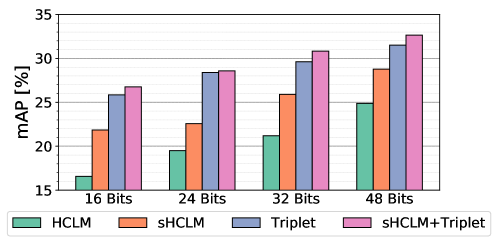
(a) Retrieval performance (mAP).

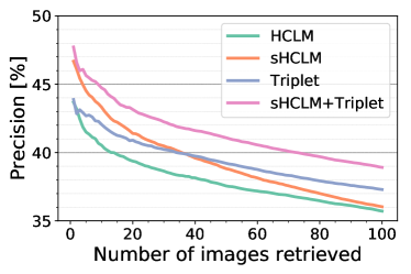
(b) Precision at K.

Figure 5: Retrieval performance on 25 unseen classes of the CIFAR-100 dataset using different versions of the proposed method.

5.3 Transfer Learning Performance

We next evaluated performance under the transfer setting of Sablayrolles:SHEval . This consists of learning the embedding with one set of classes and evaluating its retrieval and classification performance on a disjoint set. Following Sablayrolles:SHEval , a 75%/25% class split was first defined. A set of training images was extracted from the 75% split and used to learn the embedding. The sHCLM proxies of Section 4.3 are only defined for these training classes, for which images were available to compute the class representations ${\bf u}_{y}$ of (19). After training, hash codes $b(\mathbf{x})$ were computed for the images of the 25% split, by forwarding the images through the network and thresholding $\nu(\mathbf{x})$. The quality of these hash codes was then evaluated in both retrieval and classification settings. For this, the hash codes were first divided into a database and a set of queries. Then, in the retrieval experiment, the database codes were ranked by similarity to each query. In the classification experiment, the database hash codes were used to train a softmax regression classifier, whose classification performance was evaluated on the query hash codes. As suggested in Sablayrolles:SHEval , all experiments were repeated over multiple 75%/25% splits. This was done by splitting the entire dataset into four 25% sets of disjoint classes and grouping them into four 75%/25% splits, in a leave-one-out fashion. All results were averaged over these four splits.

5.3.1 Ablation Study

Figures 5a and 5b compare the retrieval performance of four embeddings. “HCLM” and “sHCLM” are proxy embeddings trained with the HCLM and sHCLM proxies, respectively. “Triplet” is a triplet embedding, learned with the loss of (22), and “sHCLM+Triplet” is trained with the joint loss of (24), using sHCLM proxies. Figure 5a shows the mAP of the Hamming rankings produced by the different embeddings on the CIFAR-100 dataset. A comparison to Figure 3b shows that the gains of semantic class alignment (sHCLM) over the HCLM proxy set increase when the retrieval system has to generalize to unseen classes. This is in line with observations from the zero- and few-shot learning literature, where it is known that capturing semantic relationships between classes is critical for generalization Lampert:Attributes ; Akata:ALE ; Morgado:SCoRe .

However, the proxy embeddings tend to overfit on the training classes, under-performing the triplet embedding. This confirms previous findings from the embedding literature, where triplet embeddings are known to generalize better for applications that rely heavily on transfer, such as face identification schroff2015 ; wang2014 . Note that the addition of the triplet loss, which did not significantly improve retrieval in experiments with the same training and test classes (Tables 2 and 3), has a significant impact in the transfer setting of Figure 5a. The increased robustness of the triplet embedding against overfitting to the training classes is also evident in Figure 5b, which shows the average precision of the top $K$ retrieved images, for $32$-bits hash codes, as a function of $K$. Note that the sHCLM proxy embedding produces higher quality rankings for low values of $K$ than the triplet embedding. On the other hand, the latter has higher precision for large values of $K$. This suggests that, while the proxy embedding produces a better local clustering of the image classes, it underperforms the triplet embedding in the grouping of less similar images from each class. Overall, the combination of the sHCLM proxy and triplet embeddings achieves the best performance. This shows that the two approaches are complementary and there are benefits to an embedding based on their combination, even in the transfer setting.

Table 4: Retrieval performance (mAP) under transfer protocol on CIFAR-100 and ILSVRC-2012 datasets.

Dataset	CIFAR-100
# Bits	16 bits	32 bits	64 bits
Classical
LSH Datar:LSH	11.0	14.2	16.6
ITQ Gong:ITQ	14.4	17.3	20.1
KSH Liu:KSH	16.2	17.1	18.4
SDH Shen:SDH	12.6	15.5	14.8
ITQ-CCA Gong:ITQ	17.5	18.1	18.2
Proxy embeddings
Softmax-PQ Sablayrolles:SHEval	—	22.0	—
BHC Lin:BHC	21.9	27.9	31.7
Triplet embeddings
DTSH Wang:TripletSH	25.5	29.4	32.1
Proposed
sHCLM	22.0	26.8	31.8
sHCLM+Triplet	27.0	30.4	32.9

Dataset	ILSVRC-2012
# Bits	32 bits	64 bits	128 bits
Proxy embeddings
Softmax-PQ Sablayrolles:SHEval	—	11.4	—
BHC Lin:BHC	10.5	14.2	17.4
Triplet embeddings
DTSH Wang:TripletSH	9.3	11.6	13.5
Proposed
sHCLM	10.3	14.4	17.4
sHCLM+Triplet	12.5	16.5	19.5

Table 5: Classification performance (Acc) under transfer protocol on CIFAR-100 and ILSVRC-2012 datasets.

Dataset	CIFAR-100
Method	16 bits	32 bits	64 bits
Classical
LSH Datar:LSH	31.6	41.3	47.9
ITQ Gong:ITQ	42.7	51.6	56.3
KSH Liu:KSH	38.3	45.5	47.8
SDH Shen:SDH	35.6	42.9	46.2
ITQ-CCA Gong:ITQ	37.6	44.4	50.6
Proxy embeddings
Softmax-PQ Sablayrolles:SHEval	—	47.4	—
BHC Lin:BHC	46.3	56.4	64.2
Triplet embeddings
DTSH Wang:TripletSH	47.3	58.0	64.4
Proposed
sHCLM	47.7	57.7	65.0
sHCLM+Triplet	44.9	55.6	63.6

Dataset	ILSVRC-2012
Method	32 bits	64 bits	128 bits
Proxy embeddings
BHC Lin:BHC	32.8	42.1	50.1
Triplet embeddings
DTSH Wang:TripletSH	30.9	40.3	48.2
Proposed
sHCLM	35.4	46.1	54.5
sHCLM+Triplet	35.7	46.3	54.7

5.3.2 Comparison to prior work

The transfer performance of the proposed embedding was compared to several approaches from the literature. Sablayrolles:SHEval proposes an initial solution to the transfer setting, denoted Softmax-PQ, which learns a standard CNN classifier (AlexNet) and uses the product quantization (PQ) mechanism of Jegou:PQ to binarize the network softmax activations. Beyond this, we evaluated the transfer performance of the BHC and DTSH methods. Since these methods do not present results on unseen classes, we used the code released by the authors to train and evaluate each method under this protocol.

Retrieval:

Table 4 shows the retrieval performance on CIFAR-100 and ILSVRC-2012. In the case of ILSVRC-2012, we trained AlexNet from scratch on the 750 training classes only, to ensure that images of test classes remain unseen until evaluation. As expected, the retrieval mAP decreased significantly when compared to the non-transfer setting of Tables 2 and 3. Similarly to the findings of Figure 5a, classical methods under-performed the more recent deep learning models. Also, the triplet embedding DTSH outperforms the proxy embedding BHC and even sHCLM on CIFAR-100. However, the opposite occurs on ILSVRC-2012, where the number of classes is much larger. This is likely because, in this case, DTSH is not able to overcome the inefficiency of triplet sampling. Finally, while sHCLM overfits to the training classes, its combination with the triplet loss of (22), sHCLM+Triplet, again achieves the best overall retrieval performance, on both datasets.

Classification:

Table 5 shows the performance of a classifier trained on the binary hash codes produced by each method. The conclusions are similar to those of Table 4. The main difference is that the sHCLM proxy embedding has a classification performance much closer to that of the joint sHCLM+Triplet embedding, even outperforming the latter on CIFAR-100. This provides more evidence that proxy embeddings produce better local clusterings of the image embeddings and suggests that, when the goal is classification, there is little benefit in adding the triplet loss, even in the transfer setting.

Conclusions:

The transfer learning setting leads to a more diverse set of conclusions than the standard supervised learning setting. In fact, for transfer learning, the relative performances of different approaches can vary substantially depending on whether the task is classification or retrieval. For classification, the main conclusion from the standard supervised setting continues to hold, i.e., there is very little reason to consider any approach other than sHCML. However, for retrieval, no clear winner emerges. Triplet embeddings can sometimes outperform and sometimes underperform sHCML. Hence, in this setting, the combination of sHCML and a triplet loss is beneficial. This combination achieves state-of-the-art retrieval performance in both datasets and has significant gains over all other approaches in at least one dataset.

5.4 Learning to hash with multi-label similarities

We finally evaluate the performance of hashing without explicit similarity classes. While this scenario can manifest itself in several ways, the most common example in the literature is the NUS-WIDE multi-tag dataset NUS-WIDE . The network of Figure 1 is trained with an sHCLM proxy set, either using the binary cross-entropy loss alone (sHCLM) or the joint loss of (24) (sHCLM+Triplet). The hyper-parameter $\lambda$ was tuned by cross-validation, using $\lambda\in\{0.01,0.1,1,10,100,1000\}$. Best performances were achieved for $\lambda=1$ or $\lambda=10$, depending on the number of bits of the hash code.

Table 6 compares the retrieval performance of several methods. Note that the table differentiates the performance of retrieval on the HBMP embedding with the standard Hamming distance (denoted as HBMP bin) and with the floating point extension proposed in cakir2018hashing (HBMP). The sHCLM proxy embedding outperforms all ranking, triplet, and pair-wise embeddings that also use the Hamming distance. By combining sHCLM with a triplet loss, the proposed approach achieves the overall best performance, outperforming all methods that rely solely on binary operations for retrieval. The combination of sHCLM+triplet and the Hamming distance even performs close to HBMP cakir2018hashing which relies on floating-point operations for retrieval. Among strictly binary methods, the only competitive approach is DSDH, which itself relies on a combination of a proxy and a triplet loss.

Table 6: Retrieval performance (mAP) on NUS-WIDE.   * Performance obtained with retrieval procedures based on floating-point operations.

Method	16 bits	24 bits	32 bits	48 bits
Ranking embeddings
DSRH Zhao:DSRH	60.9	61.8	62.1	63.1
Pair-wise embeddings
DPSH Li:DPSH	71.5	72.2	73.6	74.1
HBMP bin cakir2018hashing	74.6	–	75.4	75.4
HBMP cakir2018hashing	80.4*	–	82.9*	84.1*
Triplet embeddings
DRSCH Zhang:BitScalable	61.8	62.2	62.3	62.8
DTSH Wang:TripletSH	75.6	77.6	78.5	79.9
Combinations
DSDH Li:DeepSDH	81.5	81.4	82.0	82.1
Proposed
sHCLM	79.3	80.2	80.2	80.9
sHCLM + Triplet	81.4	82.5	83.0	83.5

6 Conclusion

In this work, we considered the hashing problem. We developed an integrated understanding of classification and metric learning and have shown that the rotational ambiguity of classification and retrieval losses is a significant hurdle to the design of representations jointly optimal for classification and hashing. We then proposed a new hashing procedure, based on a set of fixed proxies, that eliminates this rotational ambiguity. An algorithm was proposed to design semantic hash-consistent large margin (sHCLM) proxies, which are nearly optimal for both classification and hashing.

An extensive experimental evaluation has provided evidence in support of several important observations. First, sHCML was shown to unequivocally advance the state-of-the-art in proxy-based hashing methods, outperforming all previous methods in four datasets, two tasks (classification and retrieval), and three hashing settings (supervised, transfer, and multi-label). Second, for the setting where proxy embeddings are most popular, namely supervised hashing, the gains were largest for the most challenging datasets (CIFAR-100 and ILSVRC), where the number of classes is larger than the dimension of the hashing code. For these datasets, sHCML, improved the retrieval performance of the previous best proxy embeddings by as much as 10 points. To the best of our knowledge, no method in the literature has comparable performance. Even the combination of sHCML with a triplet embedding was unable to achieve consistent performance improvements. Third, while proxy embeddings dominate in the classic supervised setting, this is less clear for settings where class supervision is weaker, i.e. inference has to be performed for classes unseen at training. This was the case of both the transfer learning and multi-label datasets considered in our experiments. While, in this setting, sHCML continued to dominate for classification tasks, triplet embeddings were sometimes superior for retrieval. Although no single method emerged as a winner for the retrieval task, the combination of sHCML and a triplet loss was shown to achieve state-of-the-art performance on all datasets considered.

Overall, sHCML achieved state-of-the-art results for all datasets, either by itself (supervised setting or classification tasks) or when combined with a triplet loss (retrieval tasks for settings with weak supervision). These results show that it is an important contribution to the field of proxy-based hashing embeddings. Nevertheless, they also show that none of the two main current approaches to hashing, proxy and triplet embeddings, can fully solve the problem by itself. This suggests the need for research on methods that can combine the best properties of each of these approaches. More importantly, our results show that there is a need to move beyond testing on a single hashing setting, a practice that is still common in the literature. While we are not aware of any previous work performing the now proposed joint evaluation over the supervised, transfer, and multi-label settings, we believe that the wide adaptation of this joint evaluation is critical for further advances in the hashing literature.

Appendix A Relations between classification and metric learning

Although seemingly different, metric learning and classification are closely related. To see this, consider the Bayes rule

$$P_{Y|\mathbf{X}}(y|\mathbf{x}) = \frac{P_{\mathbf{X}|Y}(\mathbf{x}|y)P_{Y}(y)}{\sum_{k}P_{\mathbf{X}|Y}(\mathbf{x}|k)P_{Y}(k)}.$$ (27)

It follows from (2) that

$$P_{\mathbf{X}|Y}(\mathbf{x}|y)P_{Y}(y)\propto_{\mathbf{x}}e^{\mathbf{w}^{T}_{y}\nu(\mathbf{x})+b_{y}}$$ (28)

where $\propto_{\mathbf{x}}$ denotes a proportional relation for each value of $\bf x$. This holds when

$$P_{\mathbf{X}|Y}(\mathbf{x}|y) = q(\mathbf{x})e^{\mathbf{w}^{T}_{y}\nu(\mathbf{x})-\psi(\mathbf{w}_{y})}$$ (29)

$$P_{Y}(y) = \frac{e^{b_{y}+\psi(\mathbf{w}_{y})}}{\sum_{k}e^{b_{k}+\psi(\mathbf{w}_{k})}},$$ (30)

where $q(\mathbf{x})$ is any non-negative function and $\psi(\mathbf{w}_{y})$ a constant such that (29) integrates to one. In this case, $P_{\mathbf{X}|Y}(\mathbf{x}|y)$ is an exponential family distribution of canonical parameter $\mathbf{w}_{y}$, sufficient statistic $\nu(\mathbf{x})$ and cumulant function $\psi(\mathbf{w}_{y})$ barndorff2014information . Further assuming, for simplicity, that the classes are balanced, i.e., $P_{Y}(y)=\frac{1}{C}\forall y$, leads to

$$b_{y}=-\psi(\mathbf{w}_{y})+\log K$$ (31)

where $K$ is a constant.

The cumulant $\psi(\mathbf{w}_{y})$ has several important properties barndorff2014information ; nelder1972generalized ; banerjee2005clustering . First, $\psi(\cdot)$ is a convex function of $\mathbf{w}_{y}$. Second, its first and second order derivatives are the mean $\nabla\psi(\mathbf{w}_{y})={\bf\mu}^{\nu}_{y}$ and co-variance $\nabla^{2}\psi(\mathbf{w}_{y})={\bf\Sigma}^{\nu}_{y}$ of $\nu(\mathbf{x})$ under class $y$. Third, $\psi(\cdot)$ has a conjugate function, convex on ${\bf\mu}^{\nu}_{y}$, given by

$$\phi({\bf\mu}^{\nu}_{y})=\mathbf{w}^{T}_{y}{\bf\mu}^{\nu}_{y}-\psi(\mathbf{w}_{y}).$$ (32)

It follows that the exponent of (29) can be re-written as

$$\mathbf{w}^{T}_{y}\nu(\mathbf{x})-\psi(\mathbf{w}_{y}) = \mathbf{w}^{T}_{y}{\bf\mu}^{\nu}_{y}-\psi(\mathbf{w}_{y})+\mathbf{w}^{T}_{y}(\nu(\mathbf{x})-{\bf\mu}^{\nu}_{y})$$ (33)

$$= \phi({\bf\mu}^{\nu}_{y})+\mathbf{w}^{T}_{y}(\nu(\mathbf{x})-{\bf\mu}^{\nu}_{y})$$

$$= \phi({\bf\mu}^{\nu}_{y})+\nabla\phi({\bf\mu}^{\nu}_{y})^{T}(\nu(\mathbf{x})-{\bf\mu}^{\nu}_{y})$$

$$= -d_{\phi}(\nu(\mathbf{x}),{\bf\mu}^{\nu}_{y})+\phi(\nu(\mathbf{x}))$$

where

$$d_{\phi}({\bf a},{\bf b})=\phi({\bf a})-\phi({\bf b})-\langle\nabla\phi({\bf b}),{\bf a}-{\bf b}\rangle$$ (34)

is the Bregman divergence between $\bf a$ and $\bf b$ associated with $\phi$. Thus, (29) can be written as

$$P_{\mathbf{X}|Y}(\mathbf{x}|y)=u(\mathbf{x})e^{-d_{\phi}(\nu(\mathbf{x}),{\bf\mu}^{\nu}_{y})}$$ (35)

where $u(\mathbf{x})=q(\mathbf{x})e^{\phi(\nu(\mathbf{x}))}$ and using (31), (30) and (27),

$$P_{Y|\mathbf{X}}(y|\mathbf{x}) = \frac{e^{-d_{\phi}(\nu(\mathbf{x}),{\bf\mu}^{\nu}_{y})}}{\sum_{k}e^{-d_{\phi}(\nu(\mathbf{x}),{\bf\mu}^{\nu}_{k})}}.$$ (36)

Hence, learning the embedding $\nu(\mathbf{x})$ with the softmax classifier of (2) endows $\cal V$ with the Bregman divergence $d_{\phi}(\nu(\mathbf{x}),{\bf\mu}^{\nu}_{y})$. From (32), it follows that

$$\nabla\psi(\mathbf{w}_{y})={\bf\mu}_{y}^{\nu}\quad\quad\quad\nabla\phi({\bf\mu}_{y}^{\nu})=\mathbf{w}_{y}.$$ (37)

Hence,

$${\bf\mu}_{y}^{\nu}=\mathbf{w}_{y}$$ (38)

if and only if

$$\nabla\psi(\mathbf{w}_{y})=\mathbf{w}_{y}\quad\quad\quad\nabla\phi({\bf\mu}_{y}^{\nu})={\bf\mu}_{y}^{\nu},$$ (39)

which holds when

$$\psi({\bf a})=\phi({\bf a})=\frac{1}{2}||{\bf a}||^{2}.$$ (40)

It can be shown that the corresponding exponential family model is the Gaussian of identity covariance and the corresponding Bregman divergence the squared Euclidean distance. Hence, ${\bf\mu}_{y}^{g}=\mathbf{w}_{y}$ if only if $d_{\phi}$ is the $L_{2}$ distance. In this case, (36) reduces to

$$P_{Y|\mathbf{X}}(y|\mathbf{x}) = \frac{e^{-d(\nu(\mathbf{x}),\mathbf{w}_{y})}}{\sum_{k}e^{-d(\nu(\mathbf{x}),\mathbf{w}_{k})}}.$$ (41)

References

- (1) Akata, Z., Perronnin, F., Harchaoui, Z., Schmid, C.: Label-embedding for attribute-based classification. In: Computer Vision and Pattern Recognition (CVPR), IEEE Conf. on (2013)
- (2) Andoni, A., Indyk, P.: Near-optimal hashing algorithms for approximate nearest neighbor in high dimensions. In: IEEE Symposium on Foundations of Computer Science (FOCS) (2006)
- (3) Babenko, A., Slesarev, A., Chigorin, A., Lempitsky, V.: Neural codes for image retrieval. In: European Conference on Computer Vision (ECCV) (2014)
- (4) Bach, J.R., Fuller, C., Gupta, A., Hampapur, A., Horowitz, B., Humphrey, R., Jain, R.C., Shu, C.F.: Virage image search engine: an open framework for image management. In: Storage and retrieval for still image and video databases IV, vol. 2670 (1996)
- (5) Banerjee, A., Merugu, S., Dhillon, I.S., Ghosh, J.: Clustering with bregman divergences. Journal of Machine Learning Research 6(Oct), 1705–1749 (2005)
- (6) Barndorff-Nielsen, O.: Information and exponential families: in statistical theory. John Wiley & Sons (2014)
- (7) Bell, S., Bala, K.: Learning visual similarity for product design with convolutional neural networks. ACM Transactions on Graphics (TOG) 34(4) (2015)
- (8) Bregman, L.M.: The relaxation method of finding the common point of convex sets and its application to the solution of problems in convex programming. USSR computational mathematics and mathematical physics 7(3), 200–217 (1967)
- (9) Cakir, F., He, K., Adel Bargal, S., Sclaroff, S.: Mihash: Online hashing with mutual information. In: International Conference on Computer Vision (ICCV) (2017)
- (10) Cakir, F., He, K., Sclaroff, S.: Hashing with binary matrix pursuit. In: Proceedings of the European Conference on Computer Vision (ECCV), pp. 332–348 (2018)
- (11) Cao, Y., Long, M., Wang, J., Zhu, H., Wen, Q.: Deep quantization network for efficient image retrieval. In: Artificial Intelligence, AAAI Conf. on (2016)
- (12) Chopra, S., Hadsell, R., LeCun, Y.: Learning a similarity metric discriminatively, with application to face verification. In: IEEE Conf. on Computer Vision and Pattern Recognition (CVPR) (2005)
- (13) Chua, T.S., Tang, J., Hong, R., Li, H., Luo, Z., Zheng, Y.T.: NUS-WIDE: A real-world web image database from national university of singapore. In: ACM Conf. on Image and Video Retrieval (CIVR) (2009)
- (14) Datar, M., Immorlica, N., Indyk, P., Mirrokni, V.S.: Locality-sensitive hashing scheme based on p-stable distributions. In: Symposium on Computational Geometry (SOCG) (2004)
- (15) Deng, J., Dong, W., Socher, R., Li, L.J., Li, K., Fei-Fei, L.: Imagenet: A large-scale hierarchical image database. In: Computer Vision and Pattern Recognition (CVPR), IEEE Conf. on (2009)
- (16) Flickner, M., Sawhney, H., Niblack, W., Ashley, J., Huang, Q., Dom, B., Gorkani, M., Hafner, J., Lee, D., Petkovic, D., et al.: Query by image and video content: the QBIC system. Computer 28(9) (1995)
- (17) Frome, A., Corrado, G.S., Shlens, J., Bengio, S., Dean, J., Mikolov, T., et al.: Devise: A deep visual-semantic embedding model. In: Advances in Neural Information Processing Systems (NIPS) (2013)
- (18) Goldberger, J., Hinton, G.E., Roweis, S.T., Salakhutdinov, R.R.: Neighbourhood components analysis. In: Advances in Neural Information Processing Systems (NIPS) (2005)
- (19) Gong, Y., Lazebnik, S., Gordo, A., Perronnin, F.: Iterative quantization: A procrustean approach to learning binary codes for large-scale image retrieval. Pattern Analysis and Machine Intelligence (PAMI), IEEE Transactions. on 35(12) (2013)
- (20) Gordo, A., Almazán, J., Revaud, J., Larlus, D.: Deep image retrieval: Learning global representations for image search. In: European Conference on Computer Vision (ECCV) (2016)
- (21) Hadsell, R., Chopra, S., LeCun, Y.: Dimensionality reduction by learning an invariant mapping. In: IEEE Conf. on Computer Vision and Pattern Recognition (CVPR) (2006)
- (22) He, K., Cakir, F., Bargal, S.A., Sclaroff, S.: Hashing as tie-aware learning to rank. In: IEEE Conf. on Computer Vision and Pattern Recognition (CVPR) (2018)
- (23) Huang, S., Xiong, Y., Zhang, Y., Wang, J.: Unsupervised triplet hashing for fast image retrieval. In: Thematic Workshops of ACM Multimedia (2017)
- (24) Jain, H., Zepeda, J., Pérez, P., Gribonval, R.: Subic: A supervised, structured binary code for image search. In: International Conference on Computer Vision (ICCV) (2017)
- (25) Jegou, H., Douze, M., Schmid, C.: Product quantization for nearest neighbor search. Pattern Analysis and Machine Intelligence (PAMI), IEEE Transactions. on 33(1) (2011)
- (26) Jiang, Q.Y., Li, W.J.: Asymmetric deep supervised hashing. In: Thirty-Second AAAI Conference on Artificial Intelligence (2018)
- (27) Krizhevsky, A.: Learning multiple layers of features from tiny images (2009)
- (28) Krizhevsky, A., Sutskever, I., Hinton, G.E.: Imagenet classification with deep convolutional neural networks. In: Advances in Neural Information Processing Systems (NIPS) (2012)
- (29) Kulis, B., Darrell, T.: Learning to hash with binary reconstructive embeddings. In: Advances in Neural Information Processing Systems (NIPS) (2009)
- (30) Lai, H., Pan, Y., Liu, Y., Yan, S.: Simultaneous feature learning and hash coding with deep neural networks. In: Computer Vision and Pattern Recognition (CVPR), IEEE Conf. on (2015)
- (31) Lampert, C.H., Nickisch, H., Harmeling, S.: Learning to detect unseen object classes by between-class attribute transfer. In: IEEE Conf. on Computer Vision and Pattern Recognition (CVPR) (2009)
- (32) Li, L., Su, H., Xing, E., Fei-Fei, L.: Object Bank: A High-Level Image Representation for Scene Classification & Semantic Feature Sparsification. In: Advances in Neural Information Processing Systems (NIPS) (2010)
- (33) Li, Q., Sun, Z., He, R., Tan, T.: Deep supervised discrete hashing. In: Advances in Neural Information Processing Systems (NIPS) (2017)
- (34) Li, W.J., Wang, S., Kang, W.C.: Feature learning based deep supervised hashing with pairwise labels. In: Artificial Intelligence, AAAI Conf. on (2016)
- (35) Lin, K., Lu, J., Chen, C.S., Zhou, J.: Learning compact binary descriptors with unsupervised deep neural networks. In: Computer Vision and Pattern Recognition (CVPR), IEEE Conf. on (2016)
- (36) Lin, K., Yang, H.F., Hsiao, J.H., Chen, C.S.: Deep learning of binary hash codes for fast image retrieval. In: Computer Vision and Pattern Recognition (Workshops), IEEE Conf. on (2015)
- (37) Liong, E., Lu, J., Wang, G., Moulin, P., Zhou, J.: Deep hashing for compact binary codes learning. In: Computer Vision and Pattern Recognition (CVPR), IEEE Conf. on (2015)
- (38) Liu, H., Wang, R., Shan, S., Chen, X.: Deep supervised hashing for fast image retrieval. In: Computer Vision and Pattern Recognition (CVPR), IEEE Conf. on (2016)
- (39) Liu, W., Wang, J., Ji, R., Jiang, Y.G., Chang, S.F.: Supervised hashing with kernels. In: Computer Vision and Pattern Recognition (CVPR), IEEE Conf. on (2012)
- (40) Lu, J., Liong, V.E., Zhou, J.: Deep hashing for scalable image search. IEEE Transactions on Image Processing (TIP) 26(5) (2017)
- (41) Morgado, P., Vasconcelos, N.: Semantically consistent regularization for zero-shot recognition. In: Computer Vision and Pattern Recognition (CVPR), IEEE Conf. on (2017)
- (42) Movshovitz-Attias, Y., Toshev, A., Leung, T.K., Ioffe, S., Singh, S.: No fuss distance metric learning using proxies. In: International Conference on Computer Vision (ICCV) (2017)
- (43) Mu, Y., Yan, S.: Non-metric locality-sensitive hashing. In: AAAI Conf. on Artificial Intelligence (2010)
- (44) Nelder, J.A., Wedderburn, R.W.: Generalized linear models. Journal of the Royal Statistical Society: Series A (General) 135(3), 370–384 (1972)
- (45) Norouzi, M., Blei, D.M.: Minimal loss hashing for compact binary codes. In: Machine Learning (ICML), International Conf. on (2011)
- (46) Oh Song, H., Xiang, Y., Jegelka, S., Savarese, S.: Deep metric learning via lifted structured feature embedding. In: IEEE Conf. on Computer Vision and Pattern Recognition (CVPR) (2016)
- (47) Pereira, J.C., Vasconcelos, N.: Cross-modal domain adaptation for text-based regularization of image semantics in image retrieval systems. Computer Vision and Image Understanding 124 (2014)
- (48) Rasiwasia, N., Moreno, P., Vasconcelos, N.: Bridging the gap: Query by semantic example. IEEE Transactions on Multimedia 9(5) (2007)
- (49) Rohrbach, M., Stark, M., Schiele, B.: Evaluating knowledge transfer and zero-shot learning in a large-scale setting. In: IEEE Conf. on Computer Vision and Pattern Recognition (CVPR) (2011)
- (50) Sablayrolles, A., Douze, M., Usunier, N., Jégou, H.: How should we evaluate supervised hashing? In: Acoustics, Speech and Signal Processing (ICASSP), IEEE International Conf. on (2017)
- (51) Schroff, F., Kalenichenko, D., Philbin, J.: Facenet: A unified embedding for face recognition and clustering. In: IEEE Conf. on Computer Vision and Pattern Recognition (CVPR) (2015)
- (52) Shen, F., Shen, C., Liu, W., Tao Shen, H.: Supervised discrete hashing. In: Computer Vision and Pattern Recognition (CVPR), IEEE Conf. on (2015)
- (53) Smeulders, A., Worring, M., Santini, S., Gupta, A., Jain, R.: Content-based image retrieval at the end of the early years. IEEE Trans. on Pattern Analysis and Machine Intelligence (PAMI) 22(12) (2000)
- (54) Smith, J.R., Chang, S.F.: Visualseek: a fully automated content-based image query system. In: ACM International Conf. on Multimedia. ACM (1997)
- (55) Sohn, K.: Improved deep metric learning with multi-class n-pair loss objective. In: Advances in Neural Information Processing Systems (NIPS) (2016)
- (56) Song, H.O., Jegelka, S., Rathod, V., Murphy, K.: Learnable structured clustering framework for deep metric learning. arXiv preprint arXiv:1612.01213 (2016)
- (57) Sun, Y., Chen, Y., Wang, X., Tang, X.: Deep learning face representation by joint identification-verification. In: Advances in Neural Information Processing Systems (NIPS) (2014)
- (58) Tammes, P.: On the origin of number and arrangement of the places of exit on the surface of pollen-grains. Ph.D. thesis, University of Groningen (1930)
- (59) Torresani, L., Szummer, M., Fitzgibbon, A.: Efficient object category recognition using classemes. In: European Conference on Computer Vision (ECCV) (2010)
- (60) Wang, J., Kumar, S., Chang, S.F.: Semi-supervised hashing for scalable image retrieval. In: Computer Vision and Pattern Recognition (CVPR), IEEE Conf. on (2010)
- (61) Wang, J., Song, Y., Leung, T., Rosenberg, C., Wang, J., Philbin, J., Chen, B., Wu, Y.: Learning fine-grained image similarity with deep ranking. In: IEEE Conf. on Computer Vision and Pattern Recognition (CVPR) (2014)
- (62) Wang, X., Shi, Y., Kitani, K.M.: Deep supervised hashing with triplet labels. In: Asian Conference on Computer Vision (ACCV) (2016)
- (63) Weinberger, K.Q., Saul, L.K.: Distance metric learning for large margin nearest neighbor classification. Journal of Machine Learning Research (2009)
- (64) Weiss, Y., Torralba, A., Fergus, R.: Spectral hashing. In: Advances in Neural Information Processing Systems (NIPS) (2009)
- (65) Wen, Y., Zhang, K., Li, Z., Qiao, Y.: A discriminative feature learning approach for deep face recognition. In: European Conference on Computer Vision (ECCV), pp. 499–515. Springer (2016)
- (66) Wright, S., Nocedal, J.: Numerical optimization. Science 35 (1999)
- (67) Xia, R., Pan, Y., Lai, H., Liu, C., Yan, S.: Supervised hashing for image retrieval via image representation learning. In: Artificial Intelligence, AAAI Conf. on (2014)
- (68) Xie, S., Tu, Z.: Holistically-nested edge detection. In: Proceedings of the IEEE international conference on computer vision, pp. 1395–1403 (2015)
- (69) Yang, H.F., Lin, K., Chen, C.S.: Supervised learning of semantics-preserving hash via deep convolutional neural networks. IEEE Trans. on Pattern Analysis and Machine Intelligence 40(2), 437–451 (2017)
- (70) Zhang, D., Wu, W., Cheng, H., Zhang, R., Dong, Z., Cai, Z.: Image-to-video person re-identification with temporally memorized similarity learning. IEEE Transactions on Circuits and Systems for Video Technology 28(10), 2622–2632 (2017)
- (71) Zhang, J., Peng, Y., Zhang, J.: Query-adaptive image retrieval by deep weighted hashing. IEEE Transactions on Multimedia (2016)
- (72) Zhang, R., Li, J., Sun, H., Ge, Y., Luo, P., Wang, X., Lin, L.: Scan: Self-and-collaborative attention network for video person re-identification. IEEE Transactions on Image Processing (2019)
- (73) Zhang, R., Lin, L., Zhang, R., Zuo, W., Zhang, L.: Bit-scalable deep hashing with regularized similarity learning for image retrieval and person re-identification. IEEE Transactions on Image Processing 24(12) (2015)
- (74) Zhao, F., Huang, Y., Wang, L., Tan, T.: Deep semantic ranking based hashing for multi-label image retrieval. In: Computer Vision and Pattern Recognition (CVPR), IEEE Conf. on (2015)
- (75) Zhong, G., Xu, H., Yang, P., Wang, S., Dong, J.: Deep hashing learning networks. In: International Joint Conf. on Neural Networks (IJCNN) (2016)
- (76) Zhu, H., Long, M., Wang, J., Cao, Y.: Deep hashing network for efficient similarity retrieval. In: Artificial Intelligence, AAAI Conf. on (2016)