The Spectral Approach to Linear Rational Expectations Models

Abstract

This paper considers linear rational expectations models in the frequency domain under general conditions. The paper develops necessary and sufficient conditions for existence and uniqueness of particular and generic systems and characterizes the space of all solutions as an affine space in the frequency domain. It is demonstrated that solutions are not generally continuous with respect to the parameters of the models, invalidating mainstream frequentist and Bayesian methods. The ill-posedness of the problem motivates regularized solutions with theoretically guaranteed uniqueness, continuity, and even differentiability properties. Regularization is illustrated in an analysis of the limiting Gaussian likelihood functions of two analytically tractable models.

JEL Classification: C10, C32, C62, E32.

Keywords: Linear rational expectations models, frequency domain, spectral representation, Wiener-Hopf factorization, regularization, Gaussian likelihood function.

1 Introduction

Spectral analysis of stationary processes is a cornerstone of time series analysis (Brockwell & Davis, 1991; Pourahmadi, 2001; Lindquist & Picci, 2015). Since its beginnings in the late 1930s, it has benefited from being at the intersection of a number of fundamental mathematical subjects including probability, functional analysis, and complex analysis (Rozanov, 1967; Nikolski, 2002; Bingham, 2012a, b). The purpose of this paper is to attempt to bring some of this rich tradition into the linear rational expectations model (LREM) literature in the form of useful theoretical results but also with applications to statistical inference.

Using the spectral representation of stationary processes due to Kolmogorov (1939, 1941b, 1941a) and Cramér (1940, 1942), this paper recasts the LREM problem in the classical Hilbert space of the frequency domain literature. This is demonstrated concretely on simple scalar models before generalizing to multivariate models. Like the structural VARMA problem, the LREM problem is equivalent to a linear system in Hilbert space. Using the factorization method of Wiener & Hopf (1931), the paper then characterizes existence and uniqueness of solutions to particular as well as generic systems, generalizing results by Onatski (2006). The set of all solutions to a given LREM is shown to be a finite dimensional affine space in the frequency domain. The dimension of this space is expressed much more simply than in Funovits (2017, 2020). It is important to note that the underlying assumptions of existence and uniqueness in this paper are weaker than in all of the previous literature on frequency domain solutions of LREMs (Whiteman, 1983; Onatski, 2006; Tan & Walker, 2015; Tan, 2019) as these works require the exogenous process to have a purely non deterministic Wold (1938) representation, an assumption that is demonstrated to be unnecessary. The weaker assumptions of this paper also permit a clear answer for why unit roots must be excluded, an aspect of the theory absent from the previous literature.

The main results of the paper concern the ill-posdeness of the LREM problem in macroeconometrics. Hadamard (1902) defines a problem to be well-posed if its solutions satisfy the conditions of existence, uniqueness, and continuous dependence on its parameters. The LREM problem is ill-posed because it violates not just the second condition but also the third. Indeed, it has long been accepted that non-uniqueness is a feature of the LREM problem and many techniques have been developed to deal with it (e.g.  Taylor (1977), McCallum (1983), Lubik & Schorfheide (2003), Farmer et al. (2015), Bianchi & Nicolò (2019)). This paper highlights the fact that non-unique solutions that have been proposed in the literature are not guaranteed to be continuous. This problem seems to be either not well understood or not fully appreciated so far; to the author’s knowledge, Sims (2007) is the only acknowledgement of this problem. The problem of discontinuity is quite serious because it invalidates mainstream econometric methodology as reviewed, for example, in Canova (2011), DeJong & Dave (2011), or Herbst & Schorfheide (2016). These methods utilize floating point arithmetic to either optimize objective functions or sample from posterior distributions; they cannot find the isolated extrema or explore the posterior probabilities with atoms generated by discontinuity of LREM solutions.

Fortunately, the literature on ill-posed problems offers an immediate solution to the problem: regularization. The idea here is that when theory is insufficient to pin down a unique solution, other information can be brought to bear. The method can be interpreted in at least two ways: (i) penalizing economically unreasonable solutions or shrinking towards economically reasonable ones or (ii) imposing prior beliefs on the frequencies of fluctuations that solutions ought to exhibit. For example, we may like to avoid solutions where certain variables vary too wildly or impose the prior that solutions to a business cycle model should exhibit fluctuations of period between 4 and 32 quarters in quarterly data. The paper provides conditions for existence and uniqueness of regularized solutions and proves that they are continuously (even differentiably) dependent on their parameters. Thus, regularized solutions can be applied in any mainstream econometric method, frequentist or Bayesian.

As an application, the paper considers two models whose limiting Gaussian likelihood functions can be derived analytically. The exercise illustrates concretely the problems of ill-posedness alluded to earlier and the ability of regularization to restore regularity and allow for both frequentist and Bayesian analyses. Thus, the recommendation for empirical analysis is to either restrict attention to unique solutions or to use regularization.

This work is related to several recent strands in the literature. Komunjer & Ng (2011), Qu & Tkachenko (2017), Kociecki & Kolasa (2018), and Al-Sadoon & Zwiernik (2019) study the identification of LREMs based on the spectral density of observables. Christiano & Vigfusson (2003), Qu & Tkachenko (2012), Sala (2015) utilize spectral domain methods for estimating LREMs using ideas that go back to Hansen & Sargent (1980). Jurado & Chahrour (2018) study the problem of subordination (what they call “recoverability”) in the context of macroeconometric models. Al-Sadoon (2018) utilizes a generalization of Wiener-Hopf factorization in order to study unstable and non-stationary solutions ot LREMs. Ephremidze, Shargorodsky & Spitkovsky (2020) provide recent results on the continuity of spectral factorization. Finally, Al-Sadoon (2020) provides numerical algorithms for computing regularized solutions.

This paper is organized as follows. Section 2 sets up the notation and reviews the fundamental concepts of spectral analysis of time series. Section 3 provides a list of examples of simple LREMs and their solutions in the frequency domain. Section 4 introduces Wiener-Hopf factorization. Section 5 sets up the LREM problem, its existence and uniqueness properties, and establishes its ill-posedness. Section 6 introduces regularized solutions. Section 7 applies mainstream methodology to simple examples and illustrates the benefits of regularization. Section 8 concludes. Sections A-D comprise the appendix. Finally, the code for reproducing the symbolic computations and graphs is available in the Mathematica notebook accompanying this paper, spectral.nb.

2 Notation and Review

We will denote by $\mathbb{Z}$, $\mathbb{R}$, and $\mathbb{C}$ the sets of integers, real numbers, and complex numbers respectively. By $\mathbb{C}^{m\times n}$ we will denote the set of $m\times n$ matrices of complex numbers. We will use $I_{n}$ to denote the identity $n\times n$ matrix. For $M\in\mathbb{C}^{m\times m}$, $\mathrm{tr}(M)=\sum_{i=1}^{m}M_{ii}$. For $M\in\mathbb{C}^{m\times n}$, $M^{\ast}$ is the conjugate transpose of $M$, and $\|M\|_{\mathbb{C}^{m\times n}}=\left(\mathrm{tr}(MM^{\ast}\right)^{1/2}$.

All random variables in this paper are defined over a single probability space $(\Omega,\mathscr{F},P)$. For a complex random variable $X$, the expectation operator is denoted by $\boldsymbol{E}X=\int_{\Omega}X(\omega)dP(\omega)$. The space $\mathscr{L}_{2}$ is defined as the Hilbert space of complex valued random variables $X$, modulo $P$-almost sure equality, such that $\boldsymbol{E}|X|^{2}<\infty$ with inner product and norm

$$\langle X,Y\rangle=\boldsymbol{E}X\overline{Y},\qquad\|X\|_{\mathscr{L}_{2}}^{2}=\langle X,X\rangle,\qquad X,Y\in\mathscr{L}_{2}.$$

Similar to other Hilbert spaces we will consider in this paper, $\mathscr{L}_{2}$ is a set of equivalence classes of functions and not a set of functions. However, mathematical convention “relegate[s] this distinction to the status of a tacit understanding” (Rudin, 1986, p. 67). Thus, we will write “$X=Y$” instead of “$X(\omega)=Y(\omega)$ for $P$-almost all $\omega\in\Omega$” and similarly for elements of all of the other Hilbert spaces we consider in this paper. The space $\mathscr{L}_{2}^{n}$ is defined as the Hilbert space of $n$-dimensional vectors of complex valued random variables $X=\left[\begin{smallmatrix}X_{1}\\ \vdots\\ X_{n}\end{smallmatrix}\right]$, $X_{j}\in\mathscr{L}_{2}$, $j=1,\ldots,n$, with the inner product and norm

$$\langle\langle X,Y\rangle\rangle=\sum_{j=1}^{n}\langle X_{j},Y_{j}\rangle,\qquad\|X\|_{\mathscr{L}_{2}^{n}}^{2}=\langle\langle X,X\rangle\rangle,\qquad X,Y\in\mathscr{L}_{2}^{n}.$$

Let the stochastic process

$$\xi=\{\xi_{t}\in\mathscr{L}_{2}^{n}:t\in\mathbb{Z}\}$$

have the property that $\boldsymbol{E}\xi_{t}$ is constant and $\boldsymbol{E}\xi_{t}\xi_{s}^{\ast}$ depends on $t$ and $s$ only through $t-s$. Such a process is known as a covariance stationary process. Given $\xi$, we may define a number of useful objects.

First, we may define $\mathscr{H}$, the closure in $\mathscr{L}_{2}$ of the set of all finite complex linear combinations of the set $\{\xi_{jt}:j=1,\ldots,n,t\in\mathbb{Z}\}$. We define $\mathscr{H}^{n}\subset\mathscr{L}_{2}^{n}$ to be the Hilbert space of all $\xi=\left[\begin{smallmatrix}\xi_{1}\\ \vdots\\ \xi_{n}\end{smallmatrix}\right]$ with $\xi_{i}\in\mathscr{H}$ for $i=1,\ldots,n$.

Traditionally, spectral analysis utilizes the forward (rather than backward) shift operator,

$$\boldsymbol{U}:\xi_{jt}\mapsto\xi_{jt+1},\qquad j=1,\ldots,n,\quad t\in\mathbb{Z}.$$

It is well known that $\boldsymbol{U}$ extends uniquely to a bijective linear map $\boldsymbol{U}:\mathscr{H}\rightarrow\mathscr{H}$ satisfying $\langle\boldsymbol{U}\xi,\boldsymbol{U}\zeta\rangle=\langle\xi,\zeta\rangle$ for all $\xi,\zeta\in\mathscr{H}$ (Lindquist & Picci, 2015, Theorem B.2.7).

We may next define the unique spectral measure $F$ on the unit circle, $\mathbb{T}$, which satisfies

$$\boldsymbol{E}\xi_{t}\xi_{s}^{\ast}=\int z^{t-s}dF,\qquad t,s\in\mathbb{Z},$$

(Lindquist & Picci, 2015, p. 80). Many books express the integral as $\int_{-\pi}^{\pi}e^{i(t-s)\lambda}dF(\lambda)$; the notation here is substantially more compact. When $F$ is absolutely continuous with respect to normalized Lebesgue measure on $\mathbb{T}$, defined by

$$\mu\left(\{e^{\mathrm{i}\lambda}:a\leq\lambda\leq b\}\right)=\frac{1}{2\pi}(b-a),\qquad 0\leq b-a\leq 2\pi,$$

then the Radon-Nikodým derivative $dF/d\mu$ is the spectral density matrix of $\xi$. Note that the spectral density of $n$-dimensional standardized white noise is $I_{n}$. Another important example of a spectral measure, is the Dirac measure at $w\in\mathbb{T}$ defined as

$$\delta_{w}(\Lambda)=\begin{cases}1,&\;w\in\Lambda,\\ 0,&\;w\not\in\Lambda,\end{cases}$$

for Borel subsets $\Lambda\subset\mathbb{T}$. Note that $F=\delta_{w}I_{n}$ is the spectral measure of a process of the form $\xi_{t}=\xi_{0}w^{t}$ for $t\in\mathbb{Z}$, with $\boldsymbol{E}\xi_{0}\xi_{0}^{\ast}=I_{n}$.

We may also define the Hilbert space $H$ of all Borel-measurable mappings $\phi:\mathbb{T}\rightarrow\mathbb{C}^{n}$, modulo $F$-almost everywhere equality such that $\int\phi dF\phi^{\ast}<\infty$ with inner product and norm

$$(\phi,\varphi)=\int\phi dF\varphi^{\ast},\qquad\|\phi\|^{2}_{H}=(\phi,\phi),\qquad\phi,\varphi\in H.$$

We define $H^{m}$ to be the Hilbert space of all $\phi=\left[\begin{smallmatrix}\phi_{1}\\ \vdots\\ \phi_{m}\end{smallmatrix}\right]$ with $\phi_{i}\in H$ for $i=1,\ldots,m$ endowed with the inner product and norm

$$((\phi,\varphi))=\sum_{j=1}^{m}(\phi_{j},\varphi_{j}),\qquad\|\phi\|^{2}_{H^{m}}=((\phi,\phi)),\qquad\phi,\varphi\in H^{m}.$$

The spectral representation theorem states that

$$\xi_{t}=\int z^{t}d\Phi,\qquad t\in\mathbb{Z},$$

for a vector of random measures $\Phi$ with $\Phi(\Lambda)\in\mathscr{H}^{n}$ and $\boldsymbol{E}\Phi(\Lambda)\Phi^{\ast}(\Lambda)=F(\Lambda)$ for Borel subsets $\Lambda\subset\mathbb{T}$ (Lindquist & Picci, 2015, Theorem 3.4.1). Many books express the integral above equivalently as $\int_{-\pi}^{\pi}e^{\mathrm{i}t\lambda}dZ(\lambda)$, where $Z(\lambda)=\Phi((-\pi,\lambda])$ for $\lambda\in(-\pi,\pi]$; again, the notation here is substantially more compact. The spectral representation theorem establishes a unitary mapping $H^{m}\rightarrow\mathscr{H}^{m}$ defined by $\phi\mapsto\xi=\int\phi d\Phi$ (Lindquist & Picci, 2015, Theorem 3.1.3). We call $\phi$ the spectral characteristic of $\xi$. Thus,

$$\left\langle\left\langle\int\phi d\Phi,\int\varphi d\Phi\right\rangle\right\rangle=((\phi,\varphi)),\qquad\phi,\varphi\in H^{m}.$$

In particular,

$$\left\|\int\phi d\Phi\right\|^{2}_{\mathscr{L}_{2}^{m}}=\|\phi\|^{2}_{H^{m}},\qquad\phi\in H^{m}.$$

Denote by $e_{j}$ the $j$-th standard basis row vector of $\mathbb{C}^{n}$. The spectral representation theorem implies that $\mathscr{H}_{t}$, the closure in $\mathscr{L}_{2}$ of the set of all finite complex linear combinations of $\{\xi_{js}:j=1,\ldots,n,s\leq t\}$, is in correspondence with the closure of the set of all finite complex linear combinations of $\{z^{s}e_{j}:j=1,\ldots,n,s\leq t\}$ in $H$, denoted $H_{t}$. $\mathscr{H}^{m}_{t}$ and $H_{t}^{m}$ are defined analogously. This implies that the orthogonal projection of $\int\phi d\Phi$ onto $\mathscr{H}^{m}_{t}$ in $\mathscr{H}^{m}$ is

$$\boldsymbol{P}\left(\int\phi d\Phi\bigg{|}\mathscr{H}^{m}_{t}\right)=\int\boldsymbol{P}(\phi|H_{t}^{m})d\Phi,\qquad t\in\mathbb{Z},$$

where $\boldsymbol{P}(\phi|H_{t}^{m})$ is the orthogonal projection of $\phi$ onto $H_{t}^{m}$ in $H^{m}$. Thus, the best linear prediction of $\xi_{jt+s}$ in terms of $\xi_{t},\xi_{t-1},\ldots$ is given by

$$\boldsymbol{P}(\xi_{jt+s}|\mathscr{H}_{t})=\int\boldsymbol{P}(z^{t+s}e_{j}|H_{t})d\Phi,\qquad s,t\in\mathbb{Z}.$$

It is easily established that $\mathscr{H}_{t}=\boldsymbol{U}^{t}\mathscr{H}_{0}$ and $H_{t}=z^{t}H_{0}$ for all $t\in\mathbb{Z}$ (Lindquist & Picci, 2015, p. 44). It follows that $\boldsymbol{P}(\boldsymbol{U}^{t}\xi|\mathscr{H}_{t})=\boldsymbol{U}^{t}\boldsymbol{P}(\xi|\mathscr{H}_{0})$ for all $\xi\in\mathscr{H}$ and likewise $\boldsymbol{P}(z^{t}\phi|H_{t})=z^{t}\boldsymbol{P}(\phi|H_{0})$ for all $\phi\in H$ (Lindquist & Picci, 2015, Lemma 2.2.9). Thus

$$\boldsymbol{P}(\xi_{t+s}|\mathscr{H}^{n}_{t})=\int z^{t}\boldsymbol{P}\left(z^{s}I_{n}|H_{0}^{n}\right)d\Phi,\qquad s,t\in\mathbb{Z}.$$

If $\zeta$ is a stochastic process such that $\{(\xi_{t}^{\prime},\zeta_{t}^{\prime})^{\prime}\in\mathscr{L}_{2}^{n+m}:t\in\mathbb{Z}\}$ is covariance stationary, we will say that $\zeta$ is causal in $\xi$ if $\zeta_{0}\in\mathscr{H}_{0}^{m}$. Finally, if $\nu$ is causal in $\xi$ and satisfies $\boldsymbol{P}(\nu_{t+1}|\mathscr{H}_{t})=0$ for all $t\in\mathbb{Z}$, we call $\nu$ an innovation process.

3 Examples

Armed with the basic machinery above, we now make a first attempt at solving LREMs in the frequency domain. We will see that solving simple univariate LREMs involves only elementary spectral domain techniques as discussed in textbook treatments of spectral analysis such as Brockwell & Davis (1991) or Pourahmadi (2001). The methods also provide strong hints to the general approach to solving LREMs. In this section, $\xi$ is a scalar covariance stationary process with $\boldsymbol{U}$, $\Phi$, $F$, $\mathscr{H}$, and $H$ defined as in the previous section.

3.1 The Autoregressive Model

We begin on familiar territory.

$$X_{t}-\alpha X_{t-1}=\xi_{t},\qquad t\in\mathbb{Z},$$ (1)

with $|\alpha|<1$. The frequency-domain analysis of this model is available in many textbooks. For completeness, we provide a treatment here that is geared towards understanding the more general cases to come.

We require a stationary solution causal in $\xi$ (further motivation of this restriction can be found in Section 5). Thus, we require

$$X_{t}=\int z^{t}\phi d\Phi,\qquad t\in\mathbb{Z},$$

for some spectral characteristic $\phi\in H_{0}$.

Notice that we may restrict attention to the equation

$$(1-\alpha\boldsymbol{U}^{-1})X_{0}=\xi_{0}.$$

If a solution to $X_{0}$ exists, then the rest of process can be generated as

$$X_{t}=\boldsymbol{U}^{t}X_{0},\qquad t\in\mathbb{Z},$$

and clearly satisfies (1).

Thus, we must solve

$$\int(1-\alpha z^{-1})\phi d\Phi=\int d\Phi.$$

In the frequency domain, we have

$$(1-\alpha z^{-1})\phi=1.$$ (2)

Since the linear mapping $\phi\mapsto\alpha z^{-1}\phi$ on $H_{0}$ is bounded in norm by $|\alpha|<1$, we see that the mapping $\phi\mapsto(1-\alpha z^{-1})\phi$ is invertible so that

$$\phi=\sum_{s=0}^{\infty}\alpha^{s}z^{-s}$$

is the unique solution to (2), where the summation is understood to converge in the $H$ sense (Gohberg et al., 2003, Theorem 2.8.1). Thus, we arrive at the unique solution to $X_{0}$,

$$X_{0} =\int\sum_{s=0}^{\infty}\alpha^{s}z^{-s}d\Phi=\sum_{s=0}^{\infty}\alpha^{s}\int z^{-s}d\Phi=\sum_{s=0}^{\infty}\alpha^{s}\xi_{-s}.$$

The interchange of the summation and the stochastic integral is admissible because the stochastic integral is a bounded linear operator mapping from $H$ to $\mathscr{H}$ and the inner summation converges in $H$. It follows that the unique stationary solution is

$$X_{t}=\boldsymbol{U}^{t}X_{0}=\sum_{s=0}^{\infty}\alpha^{s}\boldsymbol{U}^{t}\xi_{-s}=\sum_{s=0}^{\infty}\alpha^{s}\xi_{t-s},\qquad t\in\mathbb{Z}.$$

The operator $\boldsymbol{U}^{t}$ is interchangeable with the summation because it is a bounded linear operator on $\mathscr{H}$ and the summation converges in $\mathscr{L}_{2}$.

3.2 The Cagan Model

The Cagan model is given as,

$$X_{t}-\beta\boldsymbol{P}(X_{t+1}|\mathscr{H}_{t})=\xi_{t},\qquad t\in\mathbb{Z},$$ (3)

with $|\beta|<1$. Again, we look for a stationary solution causal in $\xi$ and we restrict attention to the equation

$$X_{0}-\beta\boldsymbol{P}(UX_{0}|\mathscr{H}_{0})=\xi_{0},$$

and, following a similar argument to that used above, we arrive at the underlying frequency domain problem,

$$\phi-\beta\boldsymbol{P}(z\phi|H_{0})=1.$$ (4)

Since the linear mapping $\phi\mapsto\beta\boldsymbol{P}(z\phi|H_{0})$ on $H_{0}$ is bounded in norm by $|\beta|<1$, we see that the mapping $\phi\mapsto\phi-\beta\boldsymbol{P}(z\phi|H_{0})$ is invertible so that

$$\phi=\sum_{s=0}^{\infty}\beta^{s}\boldsymbol{P}(z^{s}|H_{0})$$

is the unique solution to (4), where the summation is understood to converge in the $H$ sense (Gohberg et al., 2003, Theorem 2.8.1). Thus, we arrive at the unique solution to $X_{0}$,

$$X_{0} =\int\sum_{s=0}^{\infty}\beta^{s}\boldsymbol{P}(z^{s}|H_{0})d\Phi=\sum_{s=0}^{\infty}\beta^{s}\int\boldsymbol{P}(z^{s}|H_{0})d\Phi=\sum_{s=0}^{\infty}\beta^{s}\boldsymbol{P}(\xi_{s}|\mathscr{H}_{0}).$$

The interchange of the summation and the stochastic integral is admissible because the stochastic integral is a bounded linear operator mapping $H$ to $\mathscr{H}$ and the inner summation converges in $H$. It follows that the unique stationary solution is

$$X_{t}=\boldsymbol{U}^{t}X_{0}=\sum_{s=0}^{\infty}\beta^{s}\boldsymbol{U}^{t}\boldsymbol{P}(\xi_{s}|\mathscr{H}_{0})=\sum_{s=0}^{\infty}\beta^{s}\boldsymbol{P}(\xi_{t+s}|\mathscr{H}_{t}),\qquad t\in\mathbb{Z},$$

The operator $\boldsymbol{U}^{t}$ is interchangeable with the summation because it is a bounded linear operator on $\mathscr{H}$ and the summation converges in $\mathscr{L}_{2}$.

3.3 The Mixed Model

Now suppose we have the more general model

$$a\boldsymbol{P}(X_{t+1}|\mathscr{H}_{t})+bX_{t}+cX_{t-1}=\xi_{t},\qquad t\in\mathbb{Z},$$ (5)

where $a,b,c\in\mathbb{C}$ and $ac\neq 0$. This leads to the frequency-domain equation

$$\boldsymbol{P}((az+b+cz^{-1})\phi|H_{0})=1.$$ (6)

As noted by Sargent (1979), the solution to this system depends on the factorization of

$$M(z)=az+b+cz^{-1}=az^{-1}(z-\delta)(z-\gamma).$$

We assume, without loss of generality, that $|\gamma|\leq|\delta|$. There are four cases to consider.

Suppose $|\gamma|<1<|\delta|$. We can then write $M(z)=a(z-\delta)(1-\gamma z^{-1})$ and express the system as

$$\boldsymbol{P}((1-\delta^{-1}z)\varphi|H_{0})=1,\qquad-a\delta(1-\gamma z^{-1})\phi=\varphi.$$

The first equation can be solved as in the Cagan model (since $|\delta^{-1}|<1$), while the second can be solved as in the autoregressive model (since $|\gamma|<1$). This procedure leads us to the unique solution

$$\phi=-\frac{1}{a\delta}\sum_{u=0}^{\infty}\sum_{s=0}^{\infty}\gamma^{u}\delta^{-s}z^{-u}\boldsymbol{P}(z^{s}|H_{0})=-\frac{1}{a\delta}\sum_{u=0}^{\infty}\sum_{s=0}^{\infty}\gamma^{u}\delta^{-s}\boldsymbol{P}(z^{s-u}|H_{-u}).$$

In the time domain, we obtain the following solution

$$X_{0}=-\frac{1}{a\delta}\sum_{u=0}^{\infty}\sum_{s=0}^{\infty}\gamma^{u}\delta^{-s}\boldsymbol{P}(\xi_{s-u}|\mathscr{H}_{-u}),$$

which then gives us the general solution,

$$X_{t}=-\frac{1}{a\delta}\sum_{u=0}^{\infty}\sum_{s=0}^{\infty}\gamma^{u}\delta^{-s}\boldsymbol{P}(\xi_{s+t-u}|\mathscr{H}_{t-u}),\qquad t\in\mathbb{Z}.$$

Next, suppose that $|\delta|<1$. Then we may write $M(z)=az(1-\delta z^{-1})(1-\gamma z^{-1})$ and express our system as

$$\boldsymbol{P}(z\varphi|H_{0})=1,\qquad a(1-\delta z^{-1})(1-\gamma z^{-1})\phi=\varphi.$$

The first equation does not have a unique solution in general. For example, when $F=\mu$, then $z^{-1}+\psi$ solves the equation for any $\psi\in\mathbb{C}$. More generally, every solution is of the form

$$\varphi=z^{-1}+\psi,$$

where $\psi\in H_{0}$ with $z\psi$ orthogonal to $H_{0}$. We can then solve for $\phi$ as

$$\phi=\frac{1}{a}\sum_{u=0}^{\infty}\sum_{s=0}^{\infty}\gamma^{u}\delta^{s}z^{-s-u}(z^{-1}+\psi).$$

In the time domain, this leads to the general solution

$$X_{t}=\frac{1}{a}\sum_{u=0}^{\infty}\sum_{s=0}^{\infty}\gamma^{u}\delta^{s}(\xi_{t-s-u-1}+\nu_{t-s-u}),\qquad t\in\mathbb{Z},$$

where $\nu_{t}=\int z^{t}\psi d\Phi\in\mathscr{H}_{t}$ for $t\in\mathbb{Z}$ is an arbitrary innovation process. Indeed, $\nu_{t}\in\mathscr{H}_{t}$ for all $t\in\mathbb{Z}$ because $\psi\in H_{0}$ and $\nu_{t+1}$ is orthogonal to $\mathscr{H}_{t}$ for all $t\in\mathbb{Z}$ because $\boldsymbol{P}(\nu_{t+1}|\mathscr{H}_{t})=\int\boldsymbol{P}(z^{t+1}\psi|H_{t})d\Phi=\int z^{t}\boldsymbol{P}(z\psi|H_{0})d\Phi=0$ as $z\psi$ is orthogonal to $H_{0}$.

Now suppose $|\gamma|>1$. Then we may write $M(z)=a\delta\gamma z^{-1}(1-\delta^{-1}z)(1-\gamma^{-1}z)$ and

$$\boldsymbol{P}(a\delta\gamma(1-\delta^{-1}z)(1-\gamma^{-1}z)\varphi|H_{0})=1,\qquad z^{-1}\phi=\varphi.$$

Clearly $\varphi$ can be solved as in the Cagan model to produce

$$\varphi=\frac{1}{a\delta\gamma}\sum_{u=0}^{\infty}\sum_{s=0}^{\infty}\gamma^{-u}\delta^{-s}\boldsymbol{P}(z^{s+u}|H_{0}).$$

This implies that

$$\phi=\frac{1}{a\delta\gamma}\sum_{u=0}^{\infty}\sum_{s=0}^{\infty}\gamma^{-u}\delta^{-s}\boldsymbol{P}(z^{s+u+1}|H_{1}).$$

However, the right hand side is not generally an element of $H_{0}$. To see this, let $F=\mu$, then $\{z^{t}:t\in\mathbb{Z}\}$ is an orthonormal set and the equation above reduces to $\phi=\frac{1}{a\delta\gamma}z$, which is orthogonal to $H_{0}$.

Finally, suppose either $|\gamma|=1$ or $|\delta|=1$ so that $M(w)=0$ for some $w\in\mathbb{T}$. Then there is no solution in general, in the sense that there exist processes $\xi$ for which no stationary solution $X$ can be found. To see this, let $F=\delta_{w}$, the Dirac measure at $w$. If a solution $\phi\in H_{0}$ to (6) exists, then it must satisfy

$$\|\phi\|_{H_{0}}^{2}=\int|\phi|^{2}dF=|\phi(w)|^{2}<\infty.$$

This then implies that $M\phi=M(w)\phi(w)=0$ in $H$, which implies that $\boldsymbol{P}(M\phi|H_{0})=0$, contradicting the fact that $\boldsymbol{P}(M\phi|H_{0})=1$.

4 Wiener-Hopf Factorization

The approach we have taken in the last section is well understood in the theory of convolution equations (Gohberg & Fel’dman, 1974). The requisite factorization of $M(z)$ into two parts, a part to solve like the Cagan model and a part to solve like the autoregressive model, is known as a Wiener-Hopf factorization (Wiener & Hopf, 1931). In this section, we state the basic concepts and properties of Wiener-Hopf factorization that we will need.

Definition 1.

Let $\mathcal{W}$ be the class of functions $M:\mathbb{T}\rightarrow\mathbb{C}$ defined by

$$M(z)=\sum_{s=-\infty}^{\infty}M_{s}z^{s},$$ (7)

where $M_{s}\in\mathbb{C}$ for $s\in\mathbb{Z}$ and $\sum_{s=-\infty}^{\infty}|M_{s}|<\infty$. Define $\mathcal{W}_{\pm}\subset\mathcal{W}$ to be the class of functions (7) with $M_{s}=0$ for $s\lessgtr 0$. The sets $\mathcal{W}^{m\times n}$, $\mathcal{W}^{m\times n}_{\pm}$ are defined as the sets of matrices of size $m\times n$ populated by elements of $\mathcal{W}$ and $\mathcal{W}_{\pm}$ respectively.

The class of functions $\mathcal{W}$ is known as the Wiener algebra in the functional analysis literature (Gohberg et al., 1993, Section XXIX.2). Note that every function analytic in a neighbourhood of $\mathbb{T}$ defines an element of $\mathcal{W}$ but the opposite inclusion does not hold (e.g. $\sum_{s=0}^{\infty}s^{-2}z^{s}\in\mathcal{W}$ diverges outside $\mathbb{T}$). For $M\in\mathcal{W}^{m\times n}$, we also have that

$$\|M\|_{\infty}\leq\sum_{s=-\infty}^{\infty}\|M_{s}\|_{\mathbb{C}^{m\times n}}<\infty,$$

where $\|M\|_{\infty}$ is the $\mu$–essential supremum of $\|M(z)\|_{\mathbb{C}^{m\times n}}$.

Definition 2.

A Wiener-Hopf factorization of $M\in\mathcal{W}^{m\times m}$ is a factorization

$$M=M_{+}M_{0}M_{-},$$ (8)

where $M_{+}\in\mathcal{W}^{m\times m}_{+}$, $M_{+}^{-1}\in\mathcal{W}^{m\times m}_{+}$, $M_{-}\in\mathcal{W}^{m\times m}_{-}$, $M_{-}^{-1}\in\mathcal{W}^{m\times m}_{-}$, and $M_{0}$ is a diagonal matrix with diagonal elements $z^{\kappa_{1}},\ldots,z^{\kappa_{m}}$, where $\kappa_{1}\geq\cdots\geq\kappa_{m}$ are integers, called partial indices.

We remark that the factorization given in Definition 2 is termed a left factorization in the Wiener-Hopf factorization literature (Gohberg & Fel’dman, 1974, p. 185). It differs from the right factorization utilized in Onatski (2006) and Al-Sadoon (2018), where the roles of $M_{\pm}(z)$ are reversed. The difference is due to the fact that the present analysis works with the forward shift operator, whereas Onatski (2006) and Al-Sadoon (2018) work with the backward shift operator. A left factorization of $M$ is obtained from a right factorization of $M^{\ast}$.

Theorem 1.

Let $M\in\mathcal{W}^{m\times m}$ and suppose $\det(M(z))\neq 0$ for all $z\in\mathbb{T}$. Then $M$ has a Wiener-Hopf factorization and its partial indices are unique.

Proof.

Existence of a Wiener-Hopf factorization follows from Theorem VIII.2.2 of Gohberg & Fel’dman (1974). Uniqueness of the partial indices follows from Theorem VIII.1.1 of Gohberg & Fel’dman (1974). ∎

The condition in Theorem 1 is minimal for existence a Wiener-Hopf factorization and uniqueness of the $M_{0}$ part. The $M_{\pm}$ parts are not unique but their general form is well understood (Gohberg & Fel’dman, 1974, Theorem VIII.1.2). The non-uniqueness of $M_{\pm}$ has no bearing on any of our results. Wiener-Hopf factorizations can be computed in a variety of ways (see Rogosin & Mishuris (2016) for a recent survey).

The partial indices allow us to identify an important subset of $\mathcal{W}^{m\times m}$.

Definition 3.

Let $\mathcal{W}^{m\times m}_{\circ}$ be the subset of $M\in\mathcal{W}^{m\times m}$ such that $\det(M(z))\neq 0$ for all $z\in\mathbb{T}$ and $\kappa_{1}-\kappa_{m}\leq 1$.

When $m=1$, $0=\kappa_{1}-\kappa_{m}\leq 1$ so that $\mathcal{W}^{1\times 1}_{\circ}$ is the set of $M\in\mathcal{W}$ such that $M(z)\neq 0$ for all $z\in\mathbb{T}$. Notice that for every element of $\mathcal{W}^{m\times m}_{\circ}$, the partial indices are either all non-negative, all non-positive, or all zero. This implies that for every element of $\mathcal{W}^{m\times m}_{\circ}$,

$$\mathrm{sign}(\kappa_{i})=\mathrm{sign}\left(\sum_{i=1}^{m}\kappa_{i}\right),\qquad i=1,\ldots,m,$$

where $\mathrm{sign}$ is equal to 1, $-1$, or 0 according to whether the argument is positive, negative, or zero respectively. Since $\sum_{i=1}^{m}\kappa_{i}$ is the winding number of $\det(M(z))$ as $z$ traverses the unit circle counter-clockwise (Gohberg & Fel’dman, 1974, Theorem VIII.3.1 (c)), we can easily determine the sign of the partial indices of elements of $\mathcal{W}^{m\times m}_{\circ}$ by looking at the winding number. The importance of this fact will become clear in the next section when we combine it with the following fact.

Theorem 2.

If $\mathcal{W}^{m\times m}$ is endowed with the $\mu$–essential supremem norm then $\mathcal{W}^{m\times m}_{\circ}$ is open and dense in $\{M\in\mathcal{W}^{m\times m}:\det(M(z))\neq 0\text{ for all }z\in\mathbb{T}\}$.

Proof.

See the proof of Theorems 1.20 and 1.21 of Gohberg et al. (2003). ∎

Theorem 2 implies that the generic or typical element of $\mathcal{W}^{m\times m}$ that admits a Wiener-Hopf factorization is an element of $\mathcal{W}_{\circ}^{m\times m}$. Said differently, the elements of $\mathcal{W}^{m\times m}\backslash\mathcal{W}_{\circ}^{m\times m}$ are non-generic or exceptional in the space of Wiener-Hopf factorizable elements of $\mathcal{W}^{m\times m}$.

To see the role played by Wiener-Hopf factorization, consider system (6) again. In the first case, $M$ factorized as

$$M_{+}(z) =1-\delta^{-1}z, M_{0}(z) =1 M_{-}(z) =-a\delta(1-\gamma z^{-1}).$$

In the second case, $$M$$ factorized as

$$M_{+}(z) =1, M_{0}(z) =z M_{-}(z) =a(1-\delta z^{-1})(1-\gamma z^{-1}).$$

In the third case, $$M$$ factorized as

$$M_{+}(z) =a\delta\gamma(1-\delta^{-1}z)(1-\gamma^{-1}z), M_{0}(z) =z^{-1} M_{-}(z) =1.$$

In the fourth case, $M(w)=0$ for some $w\in\mathbb{T}$ and there does not exist a solution in general. Notice that the case of existence and uniqueness is associated with a partial index of zero, the case of existence and non-uniqueness is associated with a positive partial index, and the cases of non-existence in general is associated with a negative partial index and/or a zero of $M(z)$. These associations are not accidental as we will see in the next section.

5 Existence and Uniqueness

Given the Wiener-Hopf factorization techniques, we can now address the general LREM problem in the frequency domain. Our first task is to define existence and uniqueness of solutions to the LREM problem in the time domain.

Definition 4.

An LREM is a pair $(M,N)\in\mathcal{W}^{m\times m}\times\mathcal{W}^{m\times n}$, expressed formally as

$$\sum_{s=-\infty}^{\infty}M_{s}E_{t}X_{t+s}=\sum_{s=-\infty}^{\infty}N_{s}E_{t}\xi_{t+s},$$ (9)

where $\xi$ is exogenous and $X$ is endogenous.

The model in (9) is understood as a set of structural equations relating current, expected, and lagged values of the endogenous process $X$ to current, expected, and lagged values of exogenous economic forces $\xi$. $X$ typically consists of economic variables of interest, such as output, inflation, and the interest rate, that we seek to explain in terms of underlying economic forces $\xi$, such as shocks to technological growth or economic policy. Occasionally, researchers also consider solutions driven by sunspots, economic forces that do not appear explicitly in the system (their associated columns of $N_{s}$ are equal to zero) but are nevertheless considered to influence the behaviour of the solution; we discuss these solutions further in Section 6. The dimension of $\xi$ may be larger or, as is typically the case in modern LREMs, smaller than the dimension of $X$.

The class of models considered in Definition 5 includes the class of structural equation models ($M$ and $N$ are constant), the class of structural VARMA models ($M$ and $N$ are matrix polynomials in $z^{-1}$), and all LREMs considered in Canova (2011), DeJong & Dave (2011), and Herbst & Schorfheide (2016). For example, the model of Smets & Wouters (2007), studied in Section 6.2 of Herbst & Schorfheide (2016), consists of $m=14$ endogenous variables and $n=7$ exogenous shocks.

Now in order to endow (9) with mathematical meaning, we must first note that LREMs are distinguished among mathematical systems in that they take as inputs not only realizations of exogenous inputs $\xi$ but also a spectral measure $F$.

That is because the output $X$ of an LREM solves a system of equations in past, present, as well as expected values of $X$. In the time domain perspective on LREMs, the role of $F$ is played by a filtration with respect to which conditional expectations can be computed (Al-Sadoon, 2018, Definition 4.2). Here, conditional expectations are substituted by linear projections, the natural analogue to expectations in the frequency domain and, in order to compute projections, $F$ needs to be specified as well. We will see that the transfer function of solutions requires the triple $(M,N,F)$, while the realizations of the output require, additionally, the realizations of the inputs. In following this system-theoretic approach to LREMs, therefore, we will often use phrases such as “for every spectral measure $F$” or “for every stationary process $\xi$”.

Definition 5.

Let $\xi$ be a zero-mean, $n$-dimensional, covariance stationary process with spectral measure $F$ and let $(M,N)$ be an LREM. A solution to $(M,N)$ is an $m$-dimensional covariance stationary process $X$, causal in $\xi$, and satisfying

$$\sum_{s=-\infty}^{\infty}M_{s}\boldsymbol{P}(X_{t+s}|\mathscr{H}_{t}^{m})=\sum_{s=-\infty}^{\infty}N_{s}\boldsymbol{P}(\xi_{t+s}|\mathscr{H}_{t}^{n}),\qquad t\in\mathbb{Z},$$ (10)

where the series converge in $\mathscr{H}^{m}$. We say that $(M,N)$ has no solution in general if it is possible to find a $\xi$ such that no solution to $(M,N)$ exists. A solution $X$ is unique if whenever $Y$ is also a solution, then $X_{t}=Y_{t}$ for all $t\in\mathbb{Z}$.

By Definition 5, an LREM is a mathematical system that transforms arbitrary covariance stationary inputs into covariance stationary outputs (Kalman et al., 1969; Kailath, 1980; Sontag, 1998; Caines, 2018). The restriction to stationarity involves no loss of generality of the LREMs considered in practice as $X$ and $\xi$ typically describe deviations away from a steady state (Canova, 2011; DeJong & Dave, 2011; Herbst & Schorfheide, 2016). The mathematics of non-stationary LREMs is developed in Al-Sadoon (2018).

Definition 5 also restricts attention to causal solutions. This is because the purpose of an LREM, similarly to structural VARMA, is to explain the behaviour of economic variables in terms of past and present economic shocks and to obtain impulse responses. It makes little sense to consider models where current inflation is determined by a future shock to technology, for example. Note, however, that we do not impose invertibity of $\xi$ in terms of $X$ as it is not necessary for our purposes, although it does become necessary for estimation purposes (see Al-Sadoon & Zwiernik (2019)).

As in the previous section, it suffices to solve the $t=0$ equation

$$\sum_{s=-\infty}^{\infty}M_{s}\boldsymbol{P}(X_{s}|\mathscr{H}_{0}^{m})=\sum_{s=-\infty}^{\infty}N_{s}\boldsymbol{P}(\xi_{s}|\mathscr{H}_{0}^{n}).$$

For if $X$ is a covariance stationary process causal in $\xi$ and satisfies this system, applying the forward shift operator $t$ times to each equation we obtain (10). Of course, the forward shift operator commutes with the summation because the sum converges in $\mathscr{H}^{m}$. Let $X_{0}$ have the spectral characteristics $\phi\in H_{0}^{m}$. Then the frequency domain equivalent is

$$\sum_{s=-\infty}^{\infty}M_{s}\boldsymbol{P}(z^{s}\phi|H_{0}^{m})=\sum_{s=-\infty}^{\infty}N_{s}\boldsymbol{P}(z^{s}I_{n}|H_{0}^{n}).$$ (11)

Classical frequency domain theory is built on the backwards shift operator $\phi\mapsto z^{-1}\phi$. In order to analysis (11), we will need an additional, closely related, operator.

Definition 6.

Define $\boldsymbol{V},\boldsymbol{V}^{(-1)}:H_{0}\rightarrow H_{0}$ to be the operators

$$\boldsymbol{V}:\phi\mapsto\boldsymbol{P}(z\phi|H_{0}), \boldsymbol{V}^{(-1)}:\phi\mapsto z^{-1}\phi.$$

We write $\boldsymbol{V}^{\kappa}$ for the operator $\boldsymbol{V}$ (resp. $\boldsymbol{V}^{(-1)}$) composed with itself $\kappa\geq 1$ (resp. $-\kappa\geq 1$) times and we define $\boldsymbol{V}^{0}=\boldsymbol{I}$, the identity mapping.

The following lemma (proof omitted) lists the most important properties of $\boldsymbol{V}$ and $\boldsymbol{V}^{(-1)}$.

Lemma 1.

The operators $\boldsymbol{V}$ and $\boldsymbol{V}^{(-1)}$ have the following properties:

1. $\boldsymbol{V}^{\ast}=\boldsymbol{V}^{(-1)}$.

2. $(\boldsymbol{V}\phi,\boldsymbol{V}\phi)\leq(\phi,\phi)$ for all $\phi\in H_{0}$.

3. $\left(\boldsymbol{V}^{(-1)}\phi,\boldsymbol{V}^{(-1)}\varphi\right)=(\phi,\varphi)$ for all $\phi,\varphi\in H_{0}$.

4. $\boldsymbol{V}^{(-1)}$ is a right inverse of $\boldsymbol{V}$.

5. $\ker(\boldsymbol{V})=H_{0}\ominus z^{-1}H_{0}$.

6. $\dim\ker(\boldsymbol{V})\leq n$.

7. For all $\kappa\in\mathbb{Z}$ and $\phi\in H_{0}$, $\boldsymbol{V}^{\kappa}\phi=\boldsymbol{P}(z^{\kappa}\phi|H_{0})$.

8. For $\kappa>1$, $\ker(\boldsymbol{V}^{\kappa})=\ker(\boldsymbol{V})\oplus\boldsymbol{V}^{(-1)}\ker(\boldsymbol{V})\oplus\cdots\oplus\boldsymbol{V}^{1-\kappa}\ker(\boldsymbol{V})$.

Lemma 1 (i) states that the backwards shift operator $\boldsymbol{V}^{(-1)}$ is the adjoint of $\boldsymbol{V}$. Lemma 1 (ii) implies that the operator norm of $\boldsymbol{V}$ is bounded above by 1. Lemma 1 (iii) implies that $\boldsymbol{V}^{(-1)}$ is an isometry (Gohberg et al., 2003, Theorem X.3.1). This implies that the operator norm of $\boldsymbol{V}^{(-1)}$ is equal to 1. Lemma 1 (iv) establishes that $\boldsymbol{V}$ is right-invertible. Lemma 1 (v) clarifies the obstruction to left-invertible of $\boldsymbol{V}$ as $\ker(\boldsymbol{V})$ may be non-trivial. For example, when $F=\mu$ and $\phi\in\mathbb{C}$, then $\boldsymbol{V}^{(-1)}\boldsymbol{V}(\phi)=\boldsymbol{P}(\,\phi\,|z^{-1},z^{-2},\ldots\,)=0$. Since $H_{0}\ominus z^{-1}H_{0}$ is the set of spectral characteristics associated with innovations to $\xi$, $\ker(\boldsymbol{V})=\{0\}$ if and only if $\xi$ is purely deterministic (Lindquist & Picci, 2015, Definition 4.5.1). Lemma 1 (vi) expresses the intuitive fact that the dimension of the innovation space of a stationary process is bounded above by the dimension of the process. Lemma 1 (vii) is a convenient expression for iterates of the $\boldsymbol{V}$ operator. Finally, Lemma 1 (viii) decomposes the kernel of $\boldsymbol{V}^{\kappa}$ into a direct sum generated by the kernel of $\boldsymbol{V}$. It follows, since $\boldsymbol{V}^{(-1)}$ is an isometry, that $\dim\ker(\boldsymbol{V}^{\kappa})=\kappa\dim\ker(\boldsymbol{V})$. The time-domain analogue of the decomposition in Lemma 1 (viii) is the familiar one from Broze et al. (1985, 1995), where a process $\nu$ causal in $\xi$ satisfies

$$\boldsymbol{P}(\nu_{t+\kappa}|\mathscr{H}_{t}^{n})=0,\qquad t\in\mathbb{Z},$$

if and only if

$$\nu_{t+\kappa}=\sum_{s=1}^{\kappa}\boldsymbol{P}(\nu_{t+\kappa}|\mathscr{H}_{t+s}^{n})-\boldsymbol{P}(\nu_{t+\kappa}|\mathscr{H}_{t+s-1}^{n}),\qquad t\in\mathbb{Z}.$$

That is, if and only if $\nu_{t+\kappa}$ is representable as the sum of the prediction revisions between $t+1$ and $t+\kappa$ for all $t\in\mathbb{Z}$.

The fact that the operators $\boldsymbol{V}^{s}$ are uniformly bounded in the operator norm by 1 (Lemma 1 (i) and (ii)) ensures that $\sum_{s=-\infty}^{\infty}M_{s}\boldsymbol{V}^{s}$ is a bounded linear operator on $H_{0}$ whenever $\sum_{s=-\infty}^{\infty}M_{s}z^{s}\in\mathcal{W}$ (Gohberg et al., 1990, Theorem I.3.2). More generally, we have the following definition, adopted from Gohberg & Fel’dman (1974).

Definition 7.

For $M\in\mathcal{W}^{m\times n}$ with $ij$-th element $M_{ij}$, define $\boldsymbol{M}_{ij}:H_{0}\rightarrow H_{0}$ as

$$\boldsymbol{M}_{ij} =\sum_{s=-\infty}^{\infty}M_{sij}\boldsymbol{V}^{s},\qquad i=1,\ldots,m,\qquad j=1,\ldots,n,$$

where the series converges in the operator norm, and $\boldsymbol{M}:H_{0}^{n}\rightarrow H_{0}^{m}$ as

$$\boldsymbol{M}\phi =\left[\begin{array}[]{c}\sum_{j=1}^{n}\boldsymbol{M}_{1j}\phi_{j}\\ \vdots\\ \sum_{j=1}^{n}\boldsymbol{M}_{mj}\phi_{j}\end{array}\right]=\left[\begin{array}[]{c}\sum_{j=1}^{n}\boldsymbol{P}(M_{1j}\phi_{j}|H_{0})\\ \vdots\\ \sum_{j=1}^{n}\boldsymbol{P}(M_{mj}\phi_{j}|H_{0})\end{array}\right]=\boldsymbol{P}(M\phi|H_{0}^{m}).$$

Since $\|\boldsymbol{M}\phi\|_{H^{m}}=\|\boldsymbol{P}(M\phi|H_{0}^{m})\|_{H^{m}}\leq\|M\phi\|_{H^{m}}\leq\|M\|_{\infty}\|\phi\|_{H^{n}}$, the operator norm of $\boldsymbol{M}$ is bounded above by $\|M\|_{\infty}$. Note that by Lemma 1 (i), $\boldsymbol{M}^{\ast}:\phi\mapsto\boldsymbol{P}(M^{\ast}\phi|H_{0}^{m})$.

Definition 7 allows us to express (11) more compactly as,

$$\boldsymbol{M}\phi=\boldsymbol{N}I_{n}.$$ (12)

Recall that the spectral characteristic of $\xi$ is $I_{n}$. Thus, we have arrived at a linear equation in the Hilbert space $H_{0}^{m}$. Equations (2), (4), and (6) are special cases of (12).

As we saw in Section 3, the first step towards inverting $\boldsymbol{M}$ is to obtain a Wiener-Hopf factorization of $M$,

$$M=M_{+}M_{0}M_{-}.$$

By Theorem 1, this factorization exists if $\det(M(z))\neq 0$ for all $z\in\mathbb{T}$. Then $\boldsymbol{M}_{+}$, $\boldsymbol{M}_{0}$, and $\boldsymbol{M}_{-}$ can be defined as in Definition 7 and it is easily checked that

$$\boldsymbol{M}=\boldsymbol{M}_{+}\boldsymbol{M}_{0}\boldsymbol{M}_{-},$$

a fact that at first seems trivial until one recalls that $\boldsymbol{V}^{i}\boldsymbol{V}^{j}$ is not generally equal to $\boldsymbol{V}^{i+j}$ when $i<0<j$ (Lemma 1 (iv) and (v)). Then (12) can be broken up into a system of three equations,

$$\boldsymbol{M}_{+}\psi=\boldsymbol{N}I_{n}, \boldsymbol{M}_{0}\varphi=\psi, \boldsymbol{M}_{-}\phi=\psi.$$

The first system involves only the $\boldsymbol{V}$ operator and is solved as in the Cagan model; the third system involves only the $\boldsymbol{V}^{(-1)}$ operator and is solved as in the autoregressive model; and the second system may involve either of the operators $\boldsymbol{V}$ or $\boldsymbol{V}^{(-1)}$ and is where non-existence and non-uniqueness may arise. To see this, note that $M_{\pm}^{-1}\in\mathcal{W}^{m\times m}_{\pm}$ implies that

$$\boldsymbol{M}_{\pm}^{-1}:\phi\mapsto\boldsymbol{P}(M_{\pm}^{-1}\phi|H_{0}^{m})$$

are well defined bounded linear operators on $H_{0}^{m}$ and

$$\boldsymbol{M}_{\pm}^{-1}\boldsymbol{M}_{\pm}=\boldsymbol{M}_{\pm}\boldsymbol{M}_{\pm}^{-1}=\boldsymbol{I},$$

where $\boldsymbol{I}$ is the identity mapping on $H_{0}^{m}$. Finally, if all of the partial indices of $M$ are zero, then $\boldsymbol{M}_{0}$ is invertible (it is equal to $\boldsymbol{I}$). However, since $\boldsymbol{V}^{s}$ is generally invertible only on the right (see Lemma 1), the best we can hope for is right invertibility of $\boldsymbol{M}_{0}$ and therefore $\boldsymbol{M}$. Clearly, $\boldsymbol{M}_{0}$ is right invertible if and only if all the partial indices of $M$ are non-negative; in that case, a right inverse of $\boldsymbol{M}_{0}$ is given as

$$\boldsymbol{M}_{0}^{(-1)}=\left[\begin{array}[]{ccccc}\boldsymbol{V}^{(-\kappa_{1})}&0&\cdots&0\\ 0&\boldsymbol{V}^{(-\kappa_{2})}&\cdots&0\\ \vdots&\vdots&\ddots&\vdots\\ 0&0&\cdots&\boldsymbol{V}^{(-\kappa_{m})}\end{array}\right].$$ (17)

However, there are generally infinitely many other right inverses of $\boldsymbol{M}_{0}$. Every right inverse of $\boldsymbol{M}$ is of the form $\boldsymbol{M}_{-}^{-1}\boldsymbol{M}_{0}^{(-1)}\boldsymbol{M}_{+}^{-1}$ for some right inverse $\boldsymbol{M}_{0}^{(-1)}$ of $\boldsymbol{M}_{0}$.

The theoretical foundations for existence and uniqueness are now complete and all that remains is to apply well-known cookie-cutter results from functional analysis along with the simple techniques we employed in Section 3.

Lemma 2.

If $(M,N)$ is an LREM, $\det(M(z))\neq 0$ for all $z\in\mathbb{T}$, and $M$ has a Wiener-Hopf factorization (8), then for every spectral measure $F$ there exists a $\phi\in H_{0}^{m}$ satisfying (12) if and only if the partial indices of $M$ are non-negative. The general form of the solution is then

$$\phi=\boldsymbol{M}^{(-1)}\boldsymbol{N}I_{n}+\boldsymbol{M}_{-}^{-1}\psi,$$ (18)

where

$$\boldsymbol{M}^{(-1)}=\boldsymbol{M}_{-}^{-1}\boldsymbol{M}_{0}^{(-1)}\boldsymbol{M}_{+}^{-1},$$ (19)

$\psi\in\ker(\boldsymbol{M}_{0})$ and $\dim(\ker(\boldsymbol{M}))=\dim(\ker(\boldsymbol{V}))(\kappa_{1}+\cdots+\kappa_{m})$. The solution is unique for every spectral measure $F$ if and only if the partial indices of $M$ are all equal to zero.

Proof.

Existence, uniqueness, and the result on the dimension of $\ker(\boldsymbol{M})$ follow from Lemma 1 and Proposition $2^{\circ}$ of Section VIII.4 of Gohberg & Fel’dman (1974) applied to $M^{\ast}$. Clearly, (18) is a solution to (12). On the other hand, if $\phi$ is a solution to (12), then we may define

$$\psi=\boldsymbol{M}_{-}\phi-\boldsymbol{M}_{0}^{(-1)}\boldsymbol{M}_{+}^{-1}\boldsymbol{N}I_{n}.$$

Clearly $\psi\in H_{0}^{m}$. Finally,

$$\boldsymbol{M}_{0}\psi=\boldsymbol{M}_{0}\boldsymbol{M}_{-}\phi-\boldsymbol{M}_{+}^{-1}\boldsymbol{N}I_{n}=\boldsymbol{M}_{+}^{-1}(\boldsymbol{M}\phi-\boldsymbol{N}I_{n})=0.\qed$$

Lemma 2 provides necessary and sufficient conditions for existence and uniqueness of solutions irrespective of the exogenous inputs. This is in following with our system-theoretic approach to LREMs. Of course, restricting attention to a particular $\xi$ and $F$, we can say slightly more. For example, if the partial indices are non-negative and $F$ has the property that $\ker(\boldsymbol{V})=\{0\}$ then by Lemma 1 (viii), $\ker(\boldsymbol{M}_{0})=\{0\}$ and there is a unique solution to (12). That is to say, there can be no multiplicity of solutions for a perfectly predictable $\xi$. This point is made in a different context in Al-Sadoon (2018), p. 641.

In the special case of a structural VARMA model, Lemma 2 reduces to the classical result that if $\det(M(z))\neq 0$ for all $|z|\geq 1$, there exists a unique causal stationary solution for every spectral measure $F$ (Hannan & Deistler, 2012, Sections 1.1-1.2). This is due to the fact that in that case $M_{+}=M_{0}=I_{m}$ and $M_{-}=M$ is a Wiener-Hopf factorization of $M$. Note that the problem of uniqueness does not arise in the case of structural VARMA.

Lemma 2 states that $\ker(\boldsymbol{M})$ is made up of spectral characteristics corresponding to arbitrary innovation processes (see Appendix A for a detailed analysis of $\ker(\boldsymbol{M})$). The time-domain analogue of this result is the fact that non-unique solutions are driven by arbitrary innovation processes (Al-Sadoon, 2018, Theorem 4.1). The dimension of $\ker(\boldsymbol{M})$ is the dimension of the innovation space of $\xi$ multiplied by the winding number of $\det(M)$. This number is obtained in Funovits (2017, 2020) based on the Sims (2002) framework (see also Sorge (2019)).

Lemma 2 begs the question of what happens if zeros are present on the unit circle. This is addressed in the next result.

Lemma 3.

If $(M,N)$ is an LREM, $\det(M(w))=0$ for some $w\in\mathbb{T}$, and $\mathrm{rank}[\;M(w)\quad N(w)\;]=m$, there exists a spectral measure $F$ such that (12) has no solution.

Proof.

Let $0\neq x\in\mathbb{C}^{m}$ satisfy $x^{\ast}M(w)=0$ and choose $F=\delta_{w}I_{n}$. If a solution $\phi\in H_{0}^{m}$ to (12) exists, it must satisfy $\|\phi\|^{2}_{H^{m}}=\sum_{j=1}^{m}\int\phi_{j}dF\phi_{j}^{\ast}=\|\phi(w)\|^{2}_{\mathbb{C}^{m\times n}}<\infty$. Since $x^{\ast}M(z)\phi(z)=0$ for $F$–a.e. $z\in\mathbb{T}$, it follows that $x^{\ast}\boldsymbol{M}\phi=\boldsymbol{P}(x^{\ast}M\phi|H_{0})=0$. This implies that $0=x^{\ast}\boldsymbol{N}I_{n}=\boldsymbol{P}(x^{\ast}N|H_{0})$. Since $x^{\ast}N(z)=x^{\ast}N(w)$ for $F$–a.e. $z\in\mathbb{T}$ and $x^{\ast}N(w)\in H_{0}$, $x^{\ast}N(w)=\boldsymbol{P}(x^{\ast}N|H_{0})=0$. This implies that $x^{\ast}[\;M(w)\quad N(w)\;]=0$, a contradiction. ∎

The basic idea behind Lemma 3 is that when $\det(M(w))=0$ for some $w\in\mathbb{T}$, the system has a form of instability akin to that of a resonance frequency in a mechanical system. When such a system is subjected to an input oscillating at frequency $\arg(w)$, its output cannot be stationary. In particular, a mechanical system will oscillate with increasing amplitude until failure (Arnold, 1973, p. 183). In the parlance of system theory, the system is said to have an unstable mode (Sontag, 1998, Chapter 5).

The rank condition on $[\;M(w)\quad N(w)\;]$ in Lemma 3 permits inputs at frequency $\arg(w)$ to excite the instability in the system. In the VARMA literature it is typically assumed that $\mathrm{rank}[\;M(z)\quad N(z)\;]=m$ for all $z\in\mathbb{C}$ (Hannan & Deistler, 2012, Chapter 2). In the systems theory literature, similar conditions characterize controllability of the output in terms of the input (Kailath, 1980, Chapter 6). Without a condition of this sort, there may be no input that can excite the system’s instability. For example, the LREM $(M,N)=(1-z^{-1},1-z^{-1})$ has a solution $\phi=1$ for any $F$. Note that this condition permits oscillatory inputs to excite instability but not necessarily white noise inputs. For example, the LREM $(M,N)=(-z+3-2z^{-1},3-2z^{-1})$ has $M(1)=0$ and $N(1)=1$ so that the conditions of Lemma 3 are satisfied but the instability of the system cannot be excited by a white noise input because, as is easily checked, $\phi=1$ is a solution to (12) when $F=\mu$. It is possible to formulate a different condition on $N$ that will permit white noise inputs to excite instability in the system and, indeed, much more can be said about stability in LREMs. However, a general analysis of stability of LREMs is outside the scope of this paper and is left for future research.

To summarize.

Theorem 3.

Let $(M,N)$ be an LREM.

1. If $\det(M(z))\neq 0$ for all $z\in\mathbb{T}$, then for every covariance stationary process $\xi$ there exists a solution $X$ to $(M,N)$ if and only if the partial indices of $M$ are non-negative. The general form of the solution is

   $$X_{t}=\int z^{t}\boldsymbol{M}^{(-1)}\boldsymbol{N}I_{n}d\Phi+\int z^{t}\boldsymbol{M}_{-}^{-1}\psi d\Phi,\quad t\in\mathbb{Z},$$

   where $\boldsymbol{M}^{(-1)}$ is given in (19), $\psi\in\ker(\boldsymbol{M}_{0})$, and the dimension of the solution space is the dimension of the innovation space of $\xi$ times the winding number of $\det(M)$. The solution is unique for every $\xi$ if and only if the partial indices of $M$ are all equal to zero.

2. If $\det(M(w))=0$ for some $w\in\mathbb{T}$ and $\mathrm{rank}[\;M(w)\quad N(w)\;]=m$, then there exists no solution to $(M,N)$ in general.

Proof.

Follows from Lemmas 2 and 3 and the spectral representation theorem. ∎

The relationship between the partial indices and existence and uniqueness of solutions to LREMs was first discovered by Onatski (2006). The general expression of solutions is similar to the one obtained in Theorem 4.1 (ii) of Al-Sadoon (2018). Lubik & Schorfheide (2003), Farmer et al. (2015), Bianchi & Nicolò (2019), and Al-Sadoon (2020) provide computational methods for obtaining the solution in Theorem 3.

We can also state the following result for generic systems (i.e. systems in $\mathcal{W}^{m\times m}_{\circ}$), a more specialized version of which is also due to Onatski (2006).

Theorem 4.

For generic $M\in\mathcal{W}^{m\times m}$ with $\det(M(z))\neq 0$ for all $z\in\mathbb{T}$, there exists possibly infinitely many solutions, a unique solution, or no solution in general according to whether $\det(M(z))$ winds around the origin a positive, zero, or a negative number of times as $z$ traverses $\mathbb{T}$ counter-clockwise.

Proof.

Follows from Theorem 3 and the discussion preceding Theorem 2. ∎

In closing, it is important to note that the assumptions underlying existence and uniqueness in this paper are weaker than in all of the previous literature on frequency domain solutions of LREMs, namely the work of Whiteman (1983), Onatski (2006), Tan & Walker (2015), and Tan (2019). These works require the exogenous process to have a purely non deterministic Wold (1938) representation, an assumption that is demonstrated to be unnecessary. The weaker assumptions of this paper have also facilitated discussion of zeros of $M$, an aspect of the theory absent from the previous literature. The advantage of these stronger assumptions, however, is that they do permit very explicit expressions of solutions. See Appendix B for a more detailed discussion.

6 Ill-Posedness and Regularization

Current macroeconometric methodology obtains LREMs from theoretical consideration (e.g. inter-temporal optimization of firms and households) and imposes only the first of Hadamard’s conditions of well-posedness, existence. In this section, we show that the other two conditions, uniqueness and continuity, are violated and discuss the consequences of these violations. This leads to the development of a new regularized solution to LREMs with important regularity properties.

6.1 Non-Uniqueness

Non-uniqueness has long been a feature of the LREM problem in macroeconometrics. The first approach to non-uniqueness, proposed by Taylor (1977), chooses the solution that minimizes the variance of the price variable in the model if one exists. Taylor motivates this solution by asserting that collective rationality of the economic agents in the model will naturally lead them to coordinate their activities to achieve this solution. Unfortunately, this provides no guidance for models in which indeterminacy afflicts non-price variables.

The second approach to non-uniqueness obtains a particular solution $\boldsymbol{M}^{(-1)}\boldsymbol{N}I_{n}$ and sets $\psi=0$ in (18). This is the “minimum state variable” approach of McCallum (1983). It ought to be emphasized, however, that there are generally infinitely many ways to obtain particular solutions, one for every right inverse of $\boldsymbol{M}$. For example, in the Cagan model of Section 3 with $|\beta|>1$, $\phi\mapsto\left(\frac{z^{-1}+\psi}{z^{-1}-\beta}\right)\phi$ is a right inverse of $\boldsymbol{M}=1-\beta\boldsymbol{V}$ for every $\psi\in\ker(\boldsymbol{V})$. Thus, the concept of minimum state variable solution is not well-defined without specifying the particular right inverse to be used for the solution. Geometrically, a minimum state variable solution picks a point on $\boldsymbol{M}^{(-1)}\boldsymbol{N}I_{n}+\ker(\boldsymbol{M})$ by committing to a particular choice of right inverse to $\boldsymbol{M}$ and ignoring all other solutions (see Figure 1). From a practical perspective, solving the LREM by one algorithm may lead to one minimum state variable but a different algorithm might lead to a completely different minimum state variable solution.

Figure 1: Solutions to Linear Rational Expectations Models

Finally, the modern approach to non-uniqueness, as exemplified by Lubik & Schorfheide (2003), Farmer et al. (2015), and Bianchi & Nicolò (2019) uses the general expression in Theorem 3. Here, every solution is represented as $\boldsymbol{M}^{(-1)}\boldsymbol{N}I_{n}+\chi$, where $\chi\in\ker(\boldsymbol{M})$. That is, every solutions is represented as a particular solution plus a part generated by arbitrary innovation processes, also known as sunspots (Farmer, 1999). Both the particular solution and the sunspot are parametrized and the parameters are then estimated from data. The geometry of the spectral approach allows us to see very clearly a serious conceptual problem with this approach. Various papers in the literature claim to present evidence of the importance of sunspots as drivers of macroeconomic activity by showing that the contribution of sunspots, as measured by the size of the estimated $\chi$, is not insignificant empirically. However, it is clear from Figure 2 that the size of $\chi$ very much depends on the particular solution; by one representation, the solution is $\boldsymbol{M}^{(-1)}\boldsymbol{N}I_{n}+\chi_{1}$ and sunspots play a large role, by another representation $\boldsymbol{M}^{[-1]}\boldsymbol{N}I_{n}+\chi_{2}$ sunspots play a small role. Without a sound economic reason for the choice of particular solution, it is unclear that the contribution of sunspots is being measured correctly. Thus, the modern approach suffers from a similar difficulty as the minimum state variable approach.

Figure 2: Indeterminacy of Sunspots in Solutions to Linear Rational Expectations Models

It emerges, therefore, that the problem of non-uniqueness was never fully resolved in the macroeconometrics literature. Although sunspots have played an important role in macroeconomic theory, conceptualized as “self-fulfilling expectations” and “animal spirits,” the empirical methodology employed for measuring the contribution of sunspots rests upon an arbitrary choice of the particular solution without any economic foundations.

6.2 Discontinuity

Even if one remains unconvinced of the importance of selecting the particular solution based on sound economic reasoning, there remains the problem of discontinuity. It is an unfortunate fact that particular solutions to an LREM $(M,N)$ can be discontinuous in its parameters; this occurs when $M$ is non-generic, i.e. an element of $\mathcal{W}^{m\times m}\backslash\mathcal{W}^{m\times m}_{\circ}$. This is compounded by the fact that LREMs are typically parametrized purely on theoretical considerations, without any regard to statistical properties, so that elements of $\mathcal{W}^{m\times m}\backslash\mathcal{W}^{m\times m}_{\circ}$ are not expressly excluded (Onatski, 2006; Sims, 2007). We will illustrate this discontinuity with the simplest possible example. It is, of course, possible to illustrate discontinuity using a more realistic example based on an LREM that is used in practice but doing so comes at the cost of analytic tractability, as solving even the simplest multivariate LREMs can be quite cumbersome.

Consider the following example,

$$F=\mu I_{2},\qquad M(z,\theta)=\left[\begin{array}[]{cc}z^{2}&0\\ \theta z&1\end{array}\right],\qquad N(z)=\left[\begin{array}[]{cc}1&0\\ 0&1\end{array}\right],$$ (24)

with $\theta\in\mathbb{R}$. Thus, $\xi$ is a standardized white noise process.

In order to compute solutions we will need to obtain a Wiener-Hopf factorization,

$$M(z,\theta)=\begin{cases}\left[\begin{array}[]{cc}1&0\\ 0&1\end{array}\right]\left[\begin{array}[]{cc}z^{2}&0\\ 0&1\end{array}\right]\left[\begin{array}[]{cc}1&0\\ 0&1\end{array}\right],&\theta=0,\vspace{0.5cm}\\ \left[\begin{array}[]{cc}1&z\\ 0&\theta\end{array}\right]\left[\begin{array}[]{cc}z&0\\ 0&z\end{array}\right]\left[\begin{array}[]{cc}0&-\theta^{-1}\\ 1&\theta^{-1}z^{-1}\end{array}\right],&\theta\neq 0.\end{cases}$$

Thus, there exists a non-unique solution for every $\theta\in\mathbb{R}$. Define $\boldsymbol{M}(\theta)$ as in Definition 7, $\phi\mapsto\boldsymbol{P}(M(\,\cdot\,,\theta)\phi|H_{0}^{2})$. We will restrict attention to minimum state variable solutions (i.e. $\psi=0$ in (18)),

$$\phi(\theta)=\boldsymbol{M}(\theta)^{(-1)}\boldsymbol{N}I_{n}=\begin{cases}\left[\begin{array}[]{cc}z^{-2}&0\\ 0&1\end{array}\right],&\theta=0,\vspace{0.5cm}\\ \left[\begin{array}[]{cc}z^{-2}&\theta^{-1}z^{-1}\\ -\theta z^{-1}&0\end{array}\right],&\theta\neq 0.\end{cases}$$

The solution is clearly discontinuous at $\theta=0$. In particular,

$$\|\phi(\theta)-\phi(0)\|^{2}_{H^{2}} =\int|\theta^{-1}z^{-1}|^{2}d\mu+\int|\theta z^{-1}|^{2}d\mu+\int|1|^{2}d\mu=\theta^{-2}+\theta^{2}+1$$

tends to infinity as $\theta\rightarrow 0$. Thus, discontinuities can arise in the process of solving an LREM.

While this discontinuity may be quite jarring to readers acquainted with the LREM literature, from the Wiener-Hopf factorization literature point of view there is nothing surprising about this discontinuity. Indeed, (24) is a minor modification of the example given in Section 1.5 of Gohberg et al. (2003). The fact that only multivariate systems with non-unique solutions can exhibit this discontinuity may explain why discontinuity has not received sufficient attention in the LREM literature. The heart of the problem is that, when $m>1$, there are points in $\mathcal{W}^{m\times m}$ at which partial indices are discontinuous, these are precisely the non-generic set $\mathcal{W}^{m\times m}\backslash\mathcal{W}^{m\times m}_{\circ}$ (Gohberg et al., 2003, Corollary 1.22). That is, if $M\in\mathcal{W}^{m\times m}$ has partial indices satisfying $\kappa_{1}-\kappa_{m}>1$, then there are small (in the $\mu$–essential supremum norm) changes in $M$ that lead to a jump in $M_{0}$ and since $M$ has undergone only a small change, $M_{\pm}$ must also jump. If we then choose a fixed left inverse $\boldsymbol{M}_{0}^{(-1)}$ in the solution (18) (e.g. choosing $\boldsymbol{M}_{0}^{(-1)}$ as in (17)), then the discontinuity can affect the solution. This is, unfortunately, what is done in all existing solution algorithms (Al-Sadoon, 2018, 2020). In our example, the partial indices of $M(z,\theta)$ are $(2,0)$ for $\theta=0$ and $(1,1)$ for $\theta\neq 0$; $M(z,0)\in\mathcal{W}^{2\times 2}\backslash\mathcal{W}^{2\times 2}_{\circ}$ and $M(z,\theta)\in\mathcal{W}^{2\times 2}_{\circ}$ for $\theta\neq 0$. The discontinuity in the partial indices is what generates the discontinuity of the Wiener-Hopf factors, which in turn generates a discontinuity in the solution.

It bears emphasising that this discontinuity is a feature of the mathematical problem, it is not a feature of the particular algorithm used to solve the problem; Al-Sadoon (2020) shows how it arises in the Sims (2002) framework, Al-Sadoon (2018) shows how it arises in a linear systems framework, and Appendix C shows how it arises when solving the system by hand. It is also important to note that the discontinuity of Wiener-Hopf factorization implies that there can exist no numerically stable way to compute it generally. While the elements of $\mathcal{W}^{m\times m}_{\circ}$ can be factorized using finite precision arithmetic, the elements of $\mathcal{W}^{m\times m}\backslash\mathcal{W}^{m\times m}_{\circ}$ cannot be factorized without infinite precision. Thus, it is a non-starter to verify numerically whether a given system is generic or not in the process of estimation and inference. Note that an analogous problem arises for Jordan canonical factorization, which is discontinuous at a non-generic set of matrices in $\mathbb{C}^{m\times m}$ when $m>1$ (Horn & Johnson, 1985, pp. 127-128); there, the recommendation is to compute the Schur canonical form instead; and in the next section we will propose, similarly, to compute a different solution to the LREMs than the one provided in Theorem 3.

The continuous dependence of a model on its parameters is a necessary ingredient of all estimation and inference techniques. In Section 7 it is demonstrated that mainstream frequentist and Bayesian methods break down completely in the context of the model above.

6.3 Regularization

Having established that the LREM problem in macroeconometrics is ill-posed, we now consider how to obtain economically meaningful solutions amenable to mainstream econometric techniques.

Perhpas the most natural solution to the ill-posedness problem is to restrict attention to systems with unique solutions (i.e. LREMs $(M,N)$, where the partial indices of $M$ are equal to zero). Al-Sadoon & Zwiernik (2019) have shown that unique solutions are not only continuous in the parameters of an LREM but also analytic (see the proof of Theorem 6.2). A less restrictive solution is to allow for non-uniqueness but restrict attention to generic systems (i.e. $\mathcal{W}^{m\times m}_{\circ}$). However, genericity cannot be taken for granted as both Onatski (2006) and Sims (2007) have warned and some models may be parametrized to always fall inside $\mathcal{W}^{m\times m}\backslash\mathcal{W}^{m\times m}_{\circ}$ (interestingly, Sims (2007) is widely but erroneously considered to be a critique of Onatski (2006), see Al-Sadoon (2019)). Moreover, we need differentiability, not just continuity, in order to ensure asymptotic normality of extremum estimators (Pötscher & Prucha, 1997; Hannan & Deistler, 2012). Therefore, we opt for a more straightforward solution, regularization.

With the geometry of the spectral approach in view, one is led inexorably to consider the Tykhonov-regularized solution to (12), which minimizes the total variance, $\|X_{0}\|^{2}_{\mathscr{H}^{m}}=\|\phi\|^{2}_{H^{m}}$ among all solutions to (10),

$$\phi_{\boldsymbol{I}}=\arg\min\left\{\|\phi\|^{2}_{H^{m}}:\boldsymbol{M}\phi=\boldsymbol{N}I_{n}\right\}.$$

It can be shown that $\phi_{\boldsymbol{I}}=\boldsymbol{M}^{\dagger}\boldsymbol{N}I_{n}$, where $\boldsymbol{M}^{\dagger}$ is the Moore-Penrose inverse of $\boldsymbol{M}$ (Groetsch, 1977, p. 41). This takes a particularly simple form in our context.

Lemma 4.

If $M\in\mathcal{W}^{m\times m}$, $\det(M(z))\neq 0$ for all $z\in\mathbb{T}$, and the partial indices of $M$ are non-negative then,

$$\boldsymbol{M}^{\dagger}=\boldsymbol{M}^{\ast}(\boldsymbol{M}\boldsymbol{M}^{\ast})^{-1}.$$

Proof.

Since $\det(M(z))\neq 0$ for all $z\in\mathbb{T}$ and $\kappa_{m}\geq 0$, $\boldsymbol{M}$ is onto (Gohberg & Fel’dman, 1974, Proposition $2^{\circ}$ of Section VIII.4). It follows that $\boldsymbol{M}^{\dagger}=\boldsymbol{M}^{\ast}(\boldsymbol{M}\boldsymbol{M}^{\ast})^{\dagger}$ (Groetsch, 1977, Theorem 2.1.5). Since $\boldsymbol{M}$ is onto, $\boldsymbol{M}^{\ast}$ is one-to-one and so $(\boldsymbol{M}\boldsymbol{M}^{\ast})^{\dagger}=(\boldsymbol{M}\boldsymbol{M}^{\ast})^{-1}$. ∎

Lemma 4 implies a very simple technique for computing the Tykhonov-regularized solution. Whenever a solution to (12) exists, the Tykhonov-regularized solution is obtained as the unique solution to the auxiliary block triangular frequency domain system,

$$\left[\begin{array}[]{cc}\boldsymbol{M}\boldsymbol{M}^{\ast}&0\\ -\boldsymbol{M}^{\ast}&\boldsymbol{I}\end{array}\right]\left[\begin{array}[]{c}\varphi\\ \phi_{\boldsymbol{I}}\end{array}\right]=\left[\begin{array}[]{c}\boldsymbol{N}I_{n}\\ 0\end{array}\right].$$

This implies that whenever a solution exists, the regularized solution is obtained uniquely by solving an auxiliary LREM. For example, in the mixed model from Section 3, the Tykhonov-regularized solution is the solution $X$ to the auxiliary LREM,

$$a\overline{c}E_{t}Y_{t+2}+(a\overline{b}+b\overline{c})E_{t}Y_{t+1}+(|a|^{2}+|b|^{2})Y_{t}+|c|^{2}E_{t-1}Y_{t}+(b\overline{a}+c\overline{b})Y_{t-1}+c\overline{a}Y_{t-2}=\varepsilon_{t},$$

$$X_{t}=\overline{a}Y_{t-1}+\overline{b}Y_{t}+\overline{c}E_{t}Y_{t+1}.$$

This regularized solution exists and is unique whenever the original system satisfies the conditions for existence.

Note that when the partial indices of $M$ are all equal to zero, $\boldsymbol{M}^{\dagger}=\boldsymbol{M}^{\ast}(\boldsymbol{M}\boldsymbol{M}^{\ast})^{-1}=\boldsymbol{M}^{\ast}(\boldsymbol{M}^{\ast})^{-1}\boldsymbol{M}^{-1}=\boldsymbol{M}^{-1}$. In other words, Tykhonov-regularization has no effect if the solution is unique.

Figure 3: Regularized Solutions to Linear Rational Expectations Models

More generally, we may consider

$$\phi_{\boldsymbol{L}}\in\arg\min\left\{\|\boldsymbol{L}\phi\|^{2}_{H^{l}}:\boldsymbol{M}\phi=\boldsymbol{N}I_{n}\right\},$$

where $\boldsymbol{L}:H^{m}\rightarrow H^{l}$ is a bounded linear operator chosen by the researcher. Next, we consider economic motivation for a number of choices of $\boldsymbol{L}$.

If the researcher wishes to shrink the variance of the $i$-th component of $X$, they can set

$$\boldsymbol{L}:\phi\mapsto\phi_{i}.$$

Note that when the $i$-th component is the price variable, we obtain the Taylor (1977) solution.

One can also also shrink expected values of $X$. For example, if certain solutions obtained by the methods reviewed above yield expectations of output that are too variable relative to what one expects empirically, then one can impose this prior by using

$$\boldsymbol{L}:\phi\mapsto\boldsymbol{V}\phi_{j},$$

where $j$ is the coordinate corresponding to output in $X$.

Linear combinations of lagged, current, and expected values of coordinates of $X$ can also be shrunk similarly. The operator

$$\boldsymbol{L}:\phi\mapsto\left[\begin{array}[]{c}(\boldsymbol{V}-2\,\boldsymbol{I}+\boldsymbol{V}^{(-1)})\phi_{1}\\ \vdots\\ (\boldsymbol{V}-2\,\boldsymbol{I}+\boldsymbol{V}^{(-1)})\phi_{m}\end{array}\right]$$

shrinks the second difference of all variables, imposing smoothness on solutions, similar to the idea of the Hodrick & Prescott (1997) filter.

Note that the operators above belong to the class of operators defined in Definition 7. Thus, we can, more generally use any $L\in\mathcal{W}^{l\times m}$ to construct the weight

$$\boldsymbol{L}:\phi\mapsto\left[\begin{array}[]{c}\sum_{j=1}^{m}\boldsymbol{L}_{1j}\phi_{j}\\ \vdots\\ \sum_{j=1}^{m}\boldsymbol{L}_{lj}\phi_{j}\end{array}\right].$$

More importantly, regularization can allow the researcher to shrink across frequencies. For example, the researcher may wish to shrink the spectrum of the solution towards frequencies of between $2\pi/32$ and $2\pi/4$ corresponding to business cycle fluctuations of period 4-32 quarters in quarterly data, i.e. using

$$\boldsymbol{L}:\phi\mapsto L\phi, L(z)=\begin{cases}0,&\pi/16\leq|\arg(z)|\leq\pi/2,\\ I_{m},&\text{otherwise}.\end{cases}$$

Finally, we can consider solutions that minimize a finite weighted sum of individual criteria as reviewed above,

$$a_{1}\|\boldsymbol{L}_{1}\phi\|_{H^{l_{1}}}^{2}+\cdots+a_{d}\|\boldsymbol{L}_{d}\phi\|_{H^{l_{d}}}^{2},$$

where $\boldsymbol{L}_{i}:H^{m}\rightarrow H^{l_{i}}$ and $a_{i}>0$ for $i=1,\ldots,d$. This would allow the researcher to impose $d$ different criteria according to the weights $a_{1},\ldots,a_{d}$. This can be achieved by using

$$\boldsymbol{L}:\phi\mapsto\left[\begin{array}[]{c}\sqrt{a_{1}}\boldsymbol{L}_{1}\\ \vdots\\ \sqrt{a_{d}}\boldsymbol{L}_{d}\end{array}\right]\phi.$$

The argument for regularization is the same as employed throughout the inverse and ill-posed problems literatures: if theory is insufficient to pin down a unique continuous solution, other information can be employed. In our case, regularization allows economically meaningful shrinkage criteria to choose the best among all possible solutions or, what amounts to the same, it allows the researcher’s priors about economic behaviour to select the most appropriate solution. Regularization resolves the problem of selecting an economically grounded particular solution and, as we will soon see, also ameliorates the discontinuity problem.

Existence of regularized solutions is guaranteed whenever the given LREM satisfies the already minimal conditions for existence of solutions. That is because, according to Lemma 2, the set of all solutions is finite dimensional and so the problem of minimizing $\|\boldsymbol{L}\phi\|^{2}_{H^{l}}$ subject to $\boldsymbol{M}\phi=\boldsymbol{N}I_{n}$ reduces to a problem of minimizing a non-negative quadratic form (see Figure 3). Uniqueness of regularized solutions, on the other hand, is the subject of the next result.

Lemma 5.

If $(M,N)$ is an LREM, $\det(M(z))\neq 0$ for all $z\in\mathbb{T}$, the partial indices of $M$ are non-negative, and $\boldsymbol{L}:H^{m}\rightarrow H^{l}$ is a bounded linear operator, then for every spectral measure $F$,

$$\phi_{\boldsymbol{L}}=(\boldsymbol{I}-(\boldsymbol{L}|_{\ker(\boldsymbol{M})})^{\dagger}\boldsymbol{L})\boldsymbol{M}^{\dagger}\boldsymbol{N}I_{n},$$

where $\boldsymbol{L}|_{\ker(\boldsymbol{M})}$ is the restriction of $\boldsymbol{L}$ to $\ker(\boldsymbol{M})$, is a regularized solution to (12). This solution is unique for every spectral measure $F$ if and only if $\ker(\boldsymbol{L})\cap\ker(\boldsymbol{M})=\{0\}$.

Proof.

See Appendix D. ∎

Lemma 5 finds a representative regularized solution and proves that it is unique if and only if $\ker(\boldsymbol{L})\cap\ker(\boldsymbol{M})=\{0\}$. Geometrically, this condition requires the operator $\boldsymbol{L}$ to put weight on all directions of indeterminacy of the LREM. If $\ker(\boldsymbol{L})\cap\ker(\boldsymbol{M})\neq\{0\}$, it will be possible to perturb $\phi_{\boldsymbol{L}}$ in any direction in $\ker(\boldsymbol{L})\cap\ker(\boldsymbol{M})$ to arrive at another regularized solution and uniqueness will fail. A host of other representations of $\phi_{\boldsymbol{L}}$ are obtained in Appendix D.

Some special cases of Lemma 5 are particularly instructive. When $\ker(\boldsymbol{L})=\{0\}$, the regularized solution is unique regardless of $\boldsymbol{M}$. That is, when $\boldsymbol{L}$ puts weight on all directions in the solution space, the regularized solution is unique. An example of this is $\boldsymbol{L}=\boldsymbol{I}$, which produces the Tykhonov-regularized solution $\phi_{\boldsymbol{I}}=\boldsymbol{M}^{\dagger}\boldsymbol{N}I_{n}$. When $\ker(\boldsymbol{M})=\{0\}$ (i.e. the solution to the LREM is unique), the regularized solution is the unique solution regardless of $\boldsymbol{L}$. This is due to the fact that $(\boldsymbol{L}|_{\ker(\boldsymbol{M})})^{\dagger}$ is the zero operator (because $\boldsymbol{L}|_{\ker(\boldsymbol{M})}$ is the zero operator) and $\boldsymbol{M}^{\dagger}=\boldsymbol{M}^{-1}$ so that $\phi_{\boldsymbol{L}}=\boldsymbol{M}^{-1}\boldsymbol{N}I_{n}$, the unique solution.

Theorem 5.

If $(M,N)$ is an LREM, $\det(M(z))\neq 0$ for all $z\in\mathbb{T}$, the partial indices of $M$ are non-negative, and $\boldsymbol{L}:H^{m}\rightarrow H^{l}$ is a bounded linear operator, then for every covariance stationary process $\xi$ there exists a solution $X$ minimizing $\|\boldsymbol{L}\phi\|_{H^{l}}$ given by

$$X_{t}=\int z^{t}(\boldsymbol{I}-(\boldsymbol{L}|_{\ker(\boldsymbol{M})})^{\dagger}\boldsymbol{L})\boldsymbol{M}^{\dagger}\boldsymbol{N}I_{n}d\Phi,\quad t\in\mathbb{Z}.$$

The solution is unique for every $\xi$ if and and only if $\ker(\boldsymbol{M})\cap\ker(\boldsymbol{L})=\{0\}$.

Proof.

Follows from Lemma 5 and the spectral representation theorem. ∎

The expression for regularized solutions in Theorem 5 is primarily of theoretical interest. It will allow us to study continuity and differentiability with respect to underlying parameters. For estimation and inference, on the other hand, Al-Sadoon (2020) provides a numerical algorithm for computing regularized solutions in the Sims (2002) framework, which leads to equivalent algebraic rather than geometric criteria for existence and uniqueness.

We have shown that, with an appropriate choice of $\boldsymbol{L}$, the regularized solution can overcome the non-uniqueness problem. Our next result shows that regularized solutions also overcome the discontinuity problem. The continuity guarantee that we require for mainstream econometric methodology is not with respect to the $H^{m}$ norm but with respect to the $\mu$–essential supremum norm; see e.g. the continuity results for bounded spectral densities and the Gaussian likelihood functions in (Hannan, 1973; Deistler & Pötscher, 1984; Anderson, 1985). If we parametrize $M$ and $N$ as $M(z,\theta)$ and $N(z,\theta)$, then it is clear that we need $M(z,\theta)$ and $N(z,\theta)$ to be jointly continuous in $z$ and $\theta$. However, Green & Anderson (1987) note that this is not sufficient to ensure continuity of the Wiener-Hopf factors in the $\mu$–essential supremum norm. Thus, we use Green and Anderson’s idea of imposing control over $\frac{d}{dz}M(z,\theta)$ and $\frac{d}{dz}N(z,\theta)$.

Theorem 6.

Let $M:\mathbb{T}\times\Theta\rightarrow\mathbb{C}^{m\times m}$ and $N:\mathbb{T}\times\Theta\rightarrow\mathbb{C}^{m\times n}$. Under the conditions

1. $F=\mu I_{n}$.

2. $\Theta\subset\mathbb{R}^{d}$ is an open set and $\theta_{0}\in\Theta$.

3. $M(\,\cdot\,,\theta)$ and $N(\,\cdot\,,\theta)$ are analytic in a neighbourhood of $\mathbb{T}$ for every $\theta\in\Theta$.

4. $M(z,\theta)$, $N(z,\theta)$, $\frac{d}{dz}M(z,\theta)$, and $\frac{d}{dz}N(z,\theta)$ are jointly continuous at every $(z,\theta)\in\mathbb{T}\times\Theta$.

5. $\ker(\boldsymbol{L})\cap\ker(\boldsymbol{M}(\theta))=\{0\}$ for all $\theta\in\Theta$.

6. $\det(M(z,\theta_{0}))\neq 0$ for all $z\in\mathbb{T}$, and the partial indices of $M(z,\theta_{0})$ are all non-negative.

Then $\phi_{\boldsymbol{L}}(\theta)=(\boldsymbol{I}-(\boldsymbol{L}|_{\ker(\boldsymbol{M}(\theta))})^{\dagger}\boldsymbol{L})\boldsymbol{M}(\theta)^{\dagger}\boldsymbol{N}(\theta)I_{n}$, is continuous at $\theta_{0}$ in the $\mu$–essential supremum norm.

Proof.

See Appendix D. ∎

The assumptions of Theorem 6 are quite strong relative to the discussion so far. However, the relevant case for most macroeconometric applications is the case where $F=\mu I_{n}$, while $M(z,\theta)$ and $N(z,\theta)$ are Laurent matrix polynomials of uniformly bounded degree. Indeed, all of the LREMs in Canova (2011), DeJong & Dave (2011), or Herbst & Schorfheide (2016) are of this form. In this case, the continuity of the coefficients of $M(z,\theta)$ and $N(z,\theta)$ is sufficient to ensure conditions (iii) and (iv) of Theorem 6.

For the purpose of establishing asymptotic normality, we typically need not just continuity in the essential supremum norm but also differentiability in the essential supremum norm (i.e. the finite differential in $\theta$ converges to the infinitesimal differential in the essential supremum norm over $z\in\mathbb{T}$). This stronger form of differentiability allows us to differentiate under integrals, which appear in the asymptotics of maximum likelihood and generalized method of moments estimators. The following result provides exactly what we need.

Theorem 7.

Let $p$ be a positive integer. Under assumptions (i) – (vi) of Theorem 6 and,

1. $M(z,\theta)$, $N(z,\theta)$, $\frac{d}{dz}M(z,\theta)$, and $\frac{d}{dz}N(z,\theta)$ are jointly continuously differentiable with respect to $\theta$ of all orders up to $p$.

Then $\phi_{\boldsymbol{L}}(\theta)=(\boldsymbol{I}-(\boldsymbol{L}|_{\ker(\boldsymbol{M}(\theta))})^{\dagger}\boldsymbol{L})\boldsymbol{M}(\theta)^{\dagger}\boldsymbol{N}(\theta)I_{n}$, is continuously differentiable of order $p$ with respect to $\theta$ at $\theta_{0}$ in the $\mu$–essential supremum norm.

Proof.

See Appendix D. ∎

Condition (vii) of Theorem 7 is a direct strengthening of condition (iv) of Theorem 6. When $M(z,\theta)$ and $N(z,\theta)$ are Laurent matrix polynomials of uniformly bounded degree, as is usually the case in macroeconomic models, the $p$-th order continuous differentiability of the coefficients of $M(z,\theta)$ and $N(z,\theta)$ is sufficient to ensure this condition is satisfied.

To see Theorem 7 in action, consider the regularized solution to the example from the previous subsection. This can be obtained analytically in just a handful of steps.

$$\phi_{\boldsymbol{I}}(\theta) =\boldsymbol{M}(\theta)^{\ast}(\boldsymbol{M}(\theta)\boldsymbol{M}(\theta)^{\ast})^{-1}I_{2}$$

$$=\left[\begin{array}[]{cc}\boldsymbol{V}^{(-2)}&\theta\boldsymbol{V}^{(-1)}\\ \boldsymbol{0}&\boldsymbol{I}\end{array}\right]\left(\left[\begin{array}[]{cc}\boldsymbol{V}^{2}&\boldsymbol{0}\\ \theta\boldsymbol{V}&\boldsymbol{I}\end{array}\right]\left[\begin{array}[]{cc}\boldsymbol{V}^{(-2)}&\theta\boldsymbol{V}^{(-1)}\\ \boldsymbol{0}&\boldsymbol{I}\end{array}\right]\right)^{-1}\left[\begin{array}[]{cc}1&0\\ 0&1\end{array}\right]$$

$$=\left[\begin{array}[]{cc}\boldsymbol{V}^{(-2)}&\theta\boldsymbol{V}^{(-1)}\\ \boldsymbol{0}&\boldsymbol{I}\end{array}\right]\left[\begin{array}[]{cc}\boldsymbol{I}&\theta\boldsymbol{V}\\ \theta\boldsymbol{V}^{(-1)}&(\theta^{2}+1)\boldsymbol{I}\end{array}\right]^{-1}\left[\begin{array}[]{cc}1&0\\ 0&1\end{array}\right]$$

To invert the operator in the expression above, we note that it is of the form defined in Definition 7, with underlying $\mathcal{W}^{2\times 2}$ element, $\left[\begin{smallmatrix}1&\theta z\\ \theta z^{-1}&(\theta^{2}+1)\end{smallmatrix}\right]$. This matrix has the Wiener-Hopf factorization $\left[\begin{smallmatrix}1&\frac{\theta}{\theta^{2}+1}z\\ 0&1\end{smallmatrix}\right]\left[\begin{smallmatrix}1&0\vspace{0.1cm}\\ 0&1\end{smallmatrix}\right]\left[\begin{smallmatrix}\frac{1}{\theta^{2}+1}&0\\ \theta z^{-1}&\theta^{2}+1\end{smallmatrix}\right]$. Thus,

$$\phi_{\boldsymbol{I}}(\theta) =\left[\begin{array}[]{cc}\boldsymbol{V}^{(-2)}&\theta\boldsymbol{V}^{(-1)}\\ \boldsymbol{0}&\boldsymbol{I}\end{array}\right]\left(\left[\begin{array}[]{cc}\boldsymbol{I}&\frac{\theta}{\theta^{2}+1}\boldsymbol{V}\\ \boldsymbol{0}&\boldsymbol{I}\end{array}\right]\left[\begin{array}[]{cc}\frac{1}{\theta^{2}+1}\boldsymbol{I}&\boldsymbol{0}\\ \theta\boldsymbol{V}^{(-1)}&(\theta^{2}+1)\boldsymbol{I}\end{array}\right]\right)^{-1}\left[\begin{array}[]{cc}1&0\\ 0&1\end{array}\right]$$

$$=\left[\begin{array}[]{cc}\boldsymbol{V}^{(-2)}&\theta\boldsymbol{V}^{(-1)}\\ \boldsymbol{0}&\boldsymbol{I}\end{array}\right]\left(\left[\begin{array}[]{cc}(\theta^{2}+1)\boldsymbol{I}&\boldsymbol{0}\\ -\theta\boldsymbol{V}^{(-1)}&\frac{1}{\theta^{2}+1}\boldsymbol{I}\end{array}\right]\left[\begin{array}[]{cc}\boldsymbol{I}&-\frac{\theta}{\theta^{2}+1}\boldsymbol{V}\\ \boldsymbol{0}&\boldsymbol{I}\end{array}\right]\right)\left[\begin{array}[]{cc}1&0\\ 0&1\end{array}\right]$$

$$=\left[\begin{array}[]{cc}\boldsymbol{V}^{(-2)}&-\frac{\theta}{1+\theta^{2}}\boldsymbol{V}^{(-2)}\boldsymbol{V}+\frac{\theta}{1+\theta^{2}}\boldsymbol{V}^{(-1)}\\ -\theta\boldsymbol{V}^{(-1)}&\frac{1}{1+\theta^{2}}\boldsymbol{I}+\frac{\theta^{2}}{1+\theta^{2}}\boldsymbol{V}^{(-1)}\boldsymbol{V}\end{array}\right]\left[\begin{array}[]{cc}1&0\\ 0&1\end{array}\right]$$

$$=\left[\begin{array}[]{cc}z^{-2}&\frac{\theta}{1+\theta^{2}}z^{-1}\\ -\theta z^{-1}&\frac{1}{1+\theta^{2}}\end{array}\right],$$

where the last equality follows from the fact that $\ker(\boldsymbol{V})=\mathbb{C}^{2}$ when $F=\mu I_{2}$. As guaranteed by Theorems 6 and 7, this solution is not just continuous as a function of $\theta$ but also smooth. Note that the implicit right inverse of $\boldsymbol{M}_{0}$ in $\boldsymbol{M}^{\dagger}$ is

$$\boldsymbol{M}_{-}(\theta)\boldsymbol{M}(\theta)^{\dagger}\boldsymbol{M}_{+}(\theta)=\begin{cases}\left[\begin{array}[]{cc}\boldsymbol{V}^{(-2)}&0\\ 0&1\end{array}\right],&\theta=0,\vspace{0.5cm}\\ \left[\begin{array}[]{cc}\boldsymbol{V}^{(-1)}&\frac{1}{1+\theta^{2}}\left(\boldsymbol{V}^{(-1)}\boldsymbol{V}-\boldsymbol{I}\right)\\ \boldsymbol{0}&\boldsymbol{V}^{(-1)}\end{array}\right],&\theta\neq 0.\end{cases}$$

Thus, it is only by using a special right inverse of $\boldsymbol{M}_{0}(\theta)$ that we can absorb the effect of discontinuity in the partial indices at $\theta=0$ on the solution.

To summarize, the LREM problem in macroeconometrics is ill-posed. However, regularization produces solutions that are unique, continuous, and even smooth under very general regularity conditions.

7 The Limiting Gaussian Likelihood Function

As an application of the spectral approach to LREMs, we consider the limiting Gaussian likelihood function of solutions. We will follow mainstream methodology in disregarding uniqueness, identifiability, and invertibility in parametrizing the models we consider (see Al-Sadoon & Zwiernik (2019) for a careful parametrization that addresses all of these considerations). We will see that the limiting Gaussian likelihood function can display very irregular behaviour in the region of non-uniqueness, invalidating underlying assumptions of mainstream frequentist and Bayesian analysis. In turn, regularized solutions can avoid some of these anomalies. Of course, empirical analysis is conducted on the likelihood function or similar objective function and not its limit; however, it is easily checked that, in the examples below, all of our qualitative observations hold just as well for the empirical analogues. For the purposes of this section, we will assume that $\xi$ is purely non-deterministic with a rational spectral density of full rank; $M$ and $N$ are also rational; and $n=m$. See Appendix B for further discussion of these assumptions.

Our assumptions imply that any solution to the LREM is representable as

$$X_{t}=\sum_{s=0}^{\infty}\Xi_{s}\zeta_{t-s},\qquad t\in\mathbb{Z}$$

where $\zeta$ is an $m$-dimensional standardized white noise (not necessarily Gaussian) and the transfer function $\Xi(z)=\sum_{s=0}^{\infty}\Xi_{s}z^{-s}$ is rational with no poles on or outside $\mathbb{T}$.

Now suppose that, instead of $\Xi$, the process were thought to have a different rational transfer function, $K\in H_{0}^{m}$ with $\det(K)$ not identically zero. Then the $j$-th auto-covariance matrix according to $K$ is $\int z^{j}KK^{\ast}d\mu$. If we define $x_{T}=(X_{1}^{\prime},\ldots,X_{T}^{\prime})^{\prime}$ and let $\Sigma_{T}(K)$ be the covariance matrix of $x_{T}$ according to $K$, then the Gaussian likelihood function evaluated at $K$ is given as

$$(2\pi)^{-\frac{1}{2}mT}\det(\Sigma_{T}(K))^{-\frac{1}{2}}\exp\left\{-\frac{1}{2}x_{T}^{\prime}\Sigma_{T}(K)^{-1}x_{T}\right\}.$$

Up to a monotonic transformation, the Gaussian likelihood function is given by

$$\ell_{T}(K)=\frac{1}{T}\log\det(\Sigma_{T}(K))+\frac{1}{T}x_{T}^{\prime}\Sigma_{T}(K)^{-1}x_{T}.$$

The limit of this object is well known when $K$ is the transfer function of a Wold representation. However, this may not always be the case. For example, the Cagan model solution of Section 3 with $|\beta|>1$ and $\nu=0$ has a first impulse response of zero, which means that the transfer function of the solution is not invertible and so cannot correspond to a Wold representation. However, there always exists a $\tilde{K}\in H_{0}^{m}$ which satisfies the conditions for a Wold representation such that $\tilde{K}\tilde{K}^{\ast}=KK^{\ast}$ (Lindquist & Picci, 2015, Theorem 4.6.7). Under certain regularity conditions (Theorem 4.1.1 and Lemmas 4.2.2 and 4.2.3 of Hannan & Deistler (2012)), $\ell_{T}(K)$ converges almost surely as $T\rightarrow\infty$ to

$$\ell(K)=\log\det(\tilde{K}(\infty)\tilde{K}^{\ast}(\infty))+\int\mathrm{tr}\left\{(KK^{\ast})^{-1}(\Xi\Xi^{\ast})\right\}d\mu.$$

We will focus primarily on $\ell(K)$ as it is a good approximation of $\ell_{T}(K)$ and it can be computed analytically for simple LREMs. The computations and graphs of the subsequent subsections can be found in the Mathematica notebook accompanying this paper, spectral.nb.

7.1 The Cagan Model

Consider the limiting Gaussian likelihood function of the Cagan model from Section 3 when $F=\mu$, restricting attention to real parameters (Lubik & Schorfheide (2004) study the Gaussian likelihood of this model for a single sample). Then $M(z)=1-\beta z$ has the Weiner-Hopf factorization

$$M(z)=\begin{cases}M_{+}=1-\beta z,\quad M_{0}=1,\quad M_{+}=1,&|\beta|<1,\\ M_{+}=1,\quad M_{0}=z,\quad M_{-}=z^{-1}-\beta,&|\beta|>1.\end{cases}$$

Thus, the true model can be expressed as

$$X_{t}=\begin{cases}\zeta_{t},&|\beta_{0}|<1,\\ -\sum_{s=0}^{\infty}\beta_{0}^{-1-s}(\psi_{0}\zeta_{t-s}+\zeta_{t-s-1}),&|\beta_{0}|>1,\end{cases}$$

where we have used the fact that $\boldsymbol{P}(\zeta_{s}|\mathscr{H}_{t})=0$ for $s>t$ and $\mathscr{H}_{t}\ominus\mathscr{H}_{t-1}=\{c\zeta_{t}:c\in\mathbb{C}\}$. The spectral density of the true model is then given as

$$|\Xi(z)|^{2}=\begin{cases}1,&|\beta_{0}|<1,\\ \left|\frac{\beta_{0}^{-1}(\psi_{0}+z^{-1})}{1-\beta_{0}^{-1}z^{-1}}\right|^{2},&|\beta_{0}|>1.\end{cases}$$

Consider the limiting Gaussian likelihood function when $K$ is specified correctly with parameters $\beta$ and $\psi$ as

$$K(z,\beta,\psi)=\begin{cases}1,&|\beta|<1,\\ -\frac{\beta^{-1}(\psi+z^{-1})}{1-\beta^{-1}z^{-1}},&|\beta|>1.\end{cases}$$

We may choose the following Wold representation of $K$,

$$\tilde{K}(z,\beta,\psi)=\begin{cases}1,&|\beta|<1,\\ \frac{\beta^{-1}(\psi+z^{-1})}{1-\beta^{-1}z^{-1}},&|\beta|>1,\quad|\psi|\geq 1,\\ \frac{\beta^{-1}(1+\psi z^{-1})}{1-\beta^{-1}z^{-1}},&|\beta|>1,\quad|\psi|<1.\end{cases}$$

This implies that the limiting Gaussian likelihood function when $|\beta_{0}|<1$ is given by

$$\ell(\beta,\psi)=\begin{cases}1,&|\beta|<1,\\ \log(\beta^{-2}\psi^{2})+\int\left|\frac{1-\beta^{-1}z^{-1}}{\beta^{-1}(\psi+z^{-1})}\right|^{2}d\mu,&|\beta|>1,\quad|\psi|\geq 1,\\ \log(\beta^{-2})+\int\left|\frac{1-\beta^{-1}z^{-1}}{\beta^{-1}(1+\psi z^{-1})}\right|^{2}d\mu,&|\beta|>1,\quad|\psi|<1.\end{cases}$$

The contours of this function are plotted in Figure 4. The limiting Gaussian likelihood function diverges as the parameters approach the boundary of non-invertiblity, $\{|\beta|>1,|\psi|=1\}$ (Hannan & Deistler, 2012, p. 114); hence the white regions in the figure. The most important feature to note is the extent of non-identifiability in this model. $\ell(\beta,\psi)$ is minimized at the set $\{|\beta|<1\}\cup\{|\beta|>1,\beta=-\psi\}$, where $\ell(\beta,\psi)=1$; indeed, for $|\beta|>1$, $\tilde{K}(z,\beta,-\beta)=\frac{\beta^{-1}-z^{-1}}{1-\beta^{-1}z^{-1}}$ is an all-pass function. Compounding this non-identifiability, any algorithm tasked with either optimizing or exploring $\ell(\beta,\psi)$ is guaranteed to fail to converge if not initiated in the region $\{|\beta|<1\}\cup\{\beta<-1,\psi>1\}\cup\{\beta>1,\psi<-1\}$; it is easily checked that such algorithms will tend to either $(\pm\infty,\pm\infty)$ or $(\pm 1,\mp 1)$, none of which are in the parameter space.

Figure 4: Limiting Gaussian Likelihood Function of the Cagan Model for $|\beta_{0}|<1$ (Not Regularized).

If, on the other hand, $|\beta_{0}|>1$, then

$$\ell(\beta,\psi)=\begin{cases}\log(1^{2})+\int\left|\frac{\beta_{0}^{-1}(\psi_{0}+z^{-1})}{1-\beta_{0}^{-1}z^{-1}}\right|^{2}d\mu,&|\beta|<1,\\ \log(\beta^{-2}\psi^{2})+\int\left|\frac{1-\beta^{-1}z^{-1}}{\beta^{-1}(\psi+z^{-1})}\right|^{2}\left|\frac{\beta_{0}^{-1}(\psi_{0}+z^{-1})}{1-\beta_{0}^{-1}z^{-1}}\right|^{2}d\mu,&|\beta|>1,\quad|\psi|\geq 1,\\ \log(\beta^{-2})+\int\left|\frac{1-\beta^{-1}z^{-1}}{\beta^{-1}(1+\psi z^{-1})}\right|^{2}\left|\frac{\beta_{0}^{-1}(\psi_{0}+z^{-1})}{1-\beta_{0}^{-1}z^{-1}}\right|^{2}d\mu,&|\beta|>1,\quad|\psi|<1.\end{cases}$$

Irregularity is still a feature of $\ell(\beta,\psi)$ when $|\beta_{0}|>1$. This function is plotted in Figure 6 for $(\beta_{0},\psi_{0})=(2,2)$. Since the gradient of this function is rational in $\beta$ and $\psi$, we can obtain all of its critical points exactly (Cox et al., 2015, Section 3.1); these are the dots highlighted in the figure. In addition to the global minimizer at $(\beta_{0},\psi_{0})$, there are two local minima. Just as in the case $|\beta_{0}|<1$, if one should be so unfortunate as to initialize their algorithm in the wrong region, they will be guaranteed to fail to either optimize or explore the limiting Gaussian likelihood function. Things are made worse if $|\psi_{0}|<1$. Figure 6 plots $\ell(\beta,\psi)$ for $\beta_{0}=2$ and $\psi_{0}=-\frac{1}{2}$ (this choice will become clear shortly). In this case, $\ell(\beta,\psi)$ has two global minimizers at $(\pm 2,\mp\frac{1}{2})$.

Figure 5: Limiting Gaussian Likelihood Function of the Cagan Model for $\beta_{0}=\psi_{0}=2$ (Not Regularized).

Figure 6: Limiting Gaussian Likelihood Function of the Cagan Model for $\beta_{0}=2$, $\psi_{0}=-\frac{1}{2}$ (Not Regularized).

Consider now, the regularized solution of the Cagan model. It is easily checked that this corresponds to setting $\psi_{0}=-\beta_{0}^{-1}$ (hence the choice of $\psi_{0}$ earlier). We have,

$$\Xi(z)=\begin{cases}1,&|\beta_{0}|<1,\\ \beta_{0}^{-1}\frac{\beta_{0}^{-1}-z^{-1}}{1-\beta_{0}^{-1}z^{-1}},&|\beta_{0}|>1.\end{cases}$$

This transfer function produces a white noise process with variance $|\Xi(z)|^{2}=\beta_{0}^{-2}$. Indeed, the ratio $\frac{\beta_{0}^{-1}-z^{-1}}{1-\beta_{0}^{-1}z^{-1}}$ is an all-pass function. Therefore, if we specify $K$ correctly, then its Wold representation is

$$\tilde{K}(z,\beta)=\begin{cases}1,&|\beta|<1,\\ \beta^{-1},&|\beta|>1.\end{cases}$$

Now if $|\beta_{0}|<1$, the limiting Gaussian likelihood function is given as

$$\ell(\beta)=\begin{cases}1,&|\beta|<1,\\ \log(\beta^{-2})+\beta^{2},&|\beta|>1.\end{cases}$$

$\ell(\beta)$ is minimized at the interval $|\beta|<1$. See the left plot of Figure 7. Even though $\beta$ is still not identified, it suffers less identification failure than in the non-regularized solution.

If on the other hand, $|\beta_{0}|>1$,

$$\ell(\beta)=\begin{cases}\beta_{0}^{-2},&|\beta|<1,\\ \log(\beta^{-2})+\beta^{2}/\beta_{0}^{2},&|\beta|>1.\end{cases}$$

Here the likelihood function is multi-modal. See the right plot of Figure 7. Thus, while regularization reduces identification problems substantially, it does not fully eliminate them.

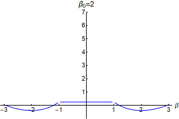
Figure 7: Limiting Gaussian Likelihood Function of the Cagan Model (Regularized).

In summary, we have found that even for the simplest of LREMs, the Cagan model, the Gaussian likelihood function exhibits some serious irregularities if the parameter space is not restricted to the region of uniqueness or the solution is not regularized. We have found that regularization helps circumvent some of these irregularities.

7.2 Non-Generic Systems

Consider now the non-generic system we studied in Section 6. The non-regularized solution is given by

$$\Xi(z)=\begin{cases}\left[\begin{array}[]{cc}z^{-2}&0\\ 0&1\end{array}\right],&\theta_{0}=0,\vspace{0.5cm}\\ \left[\begin{array}[]{cc}z^{-2}&\theta_{0}^{-1}z^{-1}\\ -\theta_{0}z^{-1}&0\end{array}\right],&\theta_{0}\neq 0.\end{cases}$$

If $K$ is correctly specified, then it has a Wold representation,

$$\tilde{K}(z,\theta)=\begin{cases}\left[\begin{array}[]{cc}1&0\\ 0&1\end{array}\right],&\theta=0,\vspace{0.5cm}\\ \left[\begin{array}[]{cc}z^{-1}&\theta^{-1}\\ -\theta&0\end{array}\right],&\theta\neq 0.\end{cases}$$

The limiting Gaussian likelihood function when $\theta_{0}=0$ is easily computed as

$$\ell(\theta)=\begin{cases}1,&\theta=0,\\ \theta^{-2}+1+\theta^{2},&\theta\neq 0.\end{cases}$$

This function is minimized at the correct value of $\theta=\theta_{0}=0$. However, it displays some very serious irregularities as seen in the left plot of Figure 9. The limiting Gaussian likelihood function is not continuous at $\theta=0$. Indeed $\lim_{0\neq\theta\rightarrow 0}\ell(\theta)=\infty$. Due to the local minima at $\pm 1$, numerical optimization algorithms will not be able to find the global minimizer and will instead converge to one of the local minimizers.

The discontinuity of the limiting Gaussian likelihood function also affects any Bayesian analysis. Mainstream Markov Chain Monte Carlo methods, as surveyed in Herbst & Schorfheide (2016) for example, require the likelihood function to be continuous. Applied to the problem at hand, these algorithms will explore the posterior around the local minimizers and fail to explore the posterior at $\theta=0$.

As these discontinuities occur at non-generic points, even plotting the empirical likelihood function or posterior will likely fail to detect them. We emphasise again that determining whether a given point is a point of discontinuity requires infinite precision, so it will not be feasible to check this numerically in the process of estimation and inference.

The limiting Gaussian likelihood function when $\theta_{0}\neq 0$ is also easily computed as

$$\ell(\theta)=\begin{cases}\theta_{0}^{-2}+1+\theta_{0}^{2},&\theta=0,\\ \theta^{2}(1+\theta_{0}^{-2})-2\theta\theta_{0}+\theta_{0}^{2}(1+\theta^{-2}),&\theta\neq 0.\end{cases}$$

This function is minimized at the correct value of $\theta=\theta_{0}$. It continues to exhibit irregularities as seen in the right plot of Figure 9. Although the function is now continuous at its global minimizer, it is still discontinuous and has a local minimum both of which can potentially lead to incorrect estimation and inference.

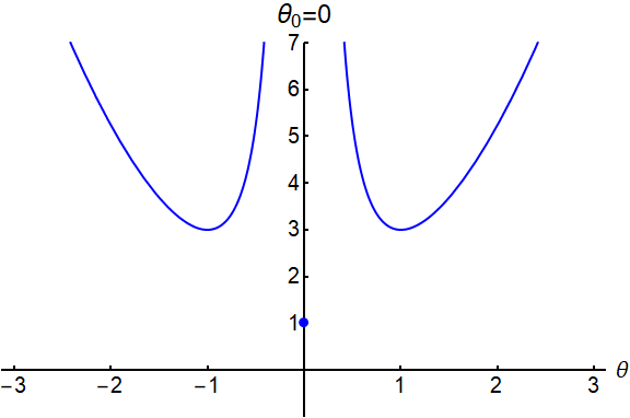
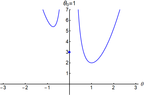
Figure 8: Limiting Gaussian Likelihood Function for the Non-Generic System (Not Regularized).

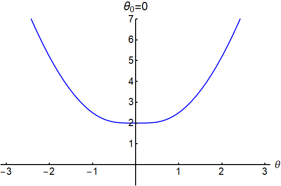
Figure 9: Limiting Gaussian Likelihood Function for the Non-Generic System (Regularized).

Consider next the regularized solution to this system.

$$\Xi(z)=\left[\begin{array}[]{cc}z^{-2}&\frac{\theta_{0}}{1+\theta_{0}^{2}}z^{-1}\\ -\theta_{0}z^{-1}&\frac{1}{1+\theta_{0}^{2}}\end{array}\right].$$

If $K$ is correctly specified, then by using elementary linear system methods (e.g. Theorem 1 of Lippi & Reichlin (1994)) it is easily shown that it has a Wold representation,

$$\tilde{K}(z,\theta)=\left[\begin{array}[]{cc}\frac{1}{\sqrt{\theta^{2}+\frac{1}{\left(\theta^{2}+1\right)^{2}}}}&-\frac{\theta^{3}\left(\theta^{2}+2\right)}{\left(\theta^{2}+1\right)^{2}\sqrt{\theta^{2}+\frac{1}{\left(\theta^{2}+1\right)^{2}}}}z^{-1}\\ 0&\sqrt{\frac{\theta^{6}+2\theta^{4}+\theta^{2}+1}{\left(\theta^{2}+1\right)^{2}}}\\ \end{array}\right].$$

The limiting Gaussian likelihood function for this model can be computed exactly and is plotted in Figure 9 for $\theta_{0}=0$ and $\theta_{0}=1$. Clearly regularization restores not just continuity but also smoothness. This is a direct corollary of Theorems 6 and 7.

In conclusion, the simple example above indicates serious problems with mainstream methodology. The assumption that a solution depends continuously on the parameters of a model is crucial for all mainstream methods of estimating LREMs as reviewed in Canova (2011), DeJong & Dave (2011), and Herbst & Schorfheide (2016). Mainstream frequentist analyses cannot allow for objective functions discontinuous at the population parameter and mainstream Bayesian analyses cannot accommodate posterior distributions with discontinuities at unknown locations. The solution is quite simple, either the parameter space should be restricted to the region of existence and uniqueness, as in Al-Sadoon & Zwiernik (2019), or regularization should be employed.

8 Conclusion

This paper has extended the LREM literature in the direction of spectral analysis. It has done so by relaxing common assumptions and developing a new regularized solution. The spectral approach has allowed us to study examples of limiting Gaussian likelihood functions of simple LREMs, which demonstrate the advantages of the new regularized solution as well as highlighting weaknesses in mainstream methodology. For the remainder, we consider some implications for future work.

The regularized solution proposed in this paper is the natural one to consider for the frequency domain. However, its motivation has been entirely econometric in nature and this begs the question of whether it can be derived from decision-theoretic foundations as proposed by Taylor (1977). Regularization has already made inroads into decision theory (Gabaix, 2014). This line of inquiry may yield other forms of regularization which may have more interesting dynamic or statistical properties.

The analysis of the Cagan model shows that the parameter space is disconnected and it can matter a great deal where one initializes their optimization routine to find the maximum likelihood estimator or their exploration routine for sampling from the posterior distribution. Therefore, it would be useful to develop simple preliminary estimators of LREMs analogous to the results for VARMA (e.g. Sections 8.4 and 11.5 of Brockwell & Davis (1991)) that can provide good initial conditions for frequentist and Bayesian algorithms.

Wiener-Hopf factorization theory has been demonstrated here and in previous work (Onatski (2006), Al-Sadoon (2018), Al-Sadoon & Zwiernik (2019)) to be the appropriate mathematical framework for analysing LREM. This begs the question of what is the appropriate framework for non-linear rational expectations models. The hope is that the mathematical insights from LREM theory will allow for important advances in non-linear modelling and inference.

Finally, researchers often rely on high-level assumptions as tentative placeholders when a result seems plausible but a proof from first principles is not apparent. Continuity of solutions to LREMs with respect to parameters has for a long time been one such high-level assumption in the LREM literature. The fact that it is generally false, should give us pause to reflect on the prevalence of this technique. At the same time, the author hopes to have conveyed a sense of optimism that theoretical progress from first principles is possible.

Appendix A Parametrizing the Set of Solutions

By Lemma 2, the set of solutions to (12) when $\kappa_{m}\geq 0$ is the affine space $\boldsymbol{M}^{(-1)}\boldsymbol{N}I_{n}+\ker(\boldsymbol{M})$, where

$$\ker(\boldsymbol{M})=\boldsymbol{M}_{-}^{-1}\ker(\boldsymbol{M}_{0}).$$

it suffices to parametrize

$$\ker(\boldsymbol{M}_{0})=\left\{\left[\begin{smallmatrix}\psi_{1}\\ \vdots\\ \psi_{m}\end{smallmatrix}\right]:\psi_{i}\in\ker(\boldsymbol{V}^{\kappa_{i}}),\;i=1,\ldots,m\right\}.$$

The problem then reduces to the parametrization of $\ker(\boldsymbol{V}^{\kappa})$ for $\kappa\geq 0$ and, by Lemma 1 (viii), the problem reduces even further to the parametrization of $\ker(\boldsymbol{V})$. Now if $\ker(\boldsymbol{V})=\{0\}$, then $\ker(\boldsymbol{V}^{\kappa})=\{0\}$ for all $\kappa\geq 0$ and so $\ker(\boldsymbol{M}_{0})=\{0\}$. If $\ker(\boldsymbol{V})\neq\{0\}$, we may find an orthonormal basis for it,

$$\Upsilon_{1},\ldots,\Upsilon_{r}\in\ker(\boldsymbol{V}).$$

Note that $r\leq n$ by Lemma 1 (vi). Lemma 1 (viii) then implies that

$$\Upsilon_{1},\ldots,\Upsilon_{r},\boldsymbol{V}^{(-1)}\Upsilon_{1},\ldots,\boldsymbol{V}^{(-1)}\Upsilon_{r},\ldots,\boldsymbol{V}^{(1-\kappa)}\Upsilon_{1},\ldots,\boldsymbol{V}^{(1-\kappa)}\Upsilon_{r}$$

is an orothonormal basis for $\ker(\boldsymbol{V}^{\kappa})$ for $\kappa\geq 0$. Thus,

$$\ker(\boldsymbol{M}_{0})=\left\{A\Upsilon:A_{ij}(z)=\sum_{s=0}^{\kappa_{i}-1}A_{sij}z^{-s},A_{sij}\in\mathbb{C},\;i=1,\ldots,m,\;j=1,\ldots,r,\;s=0,\ldots,\kappa_{i}-1\right\},$$

where

$$\Upsilon=\left[\begin{array}[]{c}\Upsilon_{1}\\ \vdots\\ \Upsilon_{r}\end{array}\right].$$

Therefore, $\ker(\boldsymbol{M}_{0})$ is the space of $m\times n$ complex matrix polynomials in $z^{-1}$, with $i$-th row degrees bounded by $\kappa_{i}-1$, multiplied by $\Upsilon$. Notice that if $M$ has $k$ partial indices at zero, then the last $k$ rows of $A$ are identically zero. The dimension of $\ker(\boldsymbol{M})$ is obtained by counting the coefficients $A_{sij}$ above, $\dim\ker(\boldsymbol{M})=r(\kappa_{1}+\cdots+\kappa_{m})$.

Appendix B Relation to Previous Literature

This section provides a review of the approaches of Whiteman (1983), Onatski (2006), Tan & Walker (2015), and Tan (2019) (henceforth, the previous literature). We will see that the previous literature makes significantly stronger assumptions about $\xi$ that also make it cumbersome to address the topic of zeros of $\det(M)$. On the other hand, the stronger assumptions do allow for very explicit expressions of solutions.

The previous literature takes as its starting point the existence of a Wold decomposition for $\xi$ with no purely deterministic part. Thus, it imposes that $F$ be absolutely continuous with respect to $\mu$ and that the spectral density matrix has an analytic spectral factorization with spectral factors of fixed rank $\mu$–a.e. (Lindquist & Picci, 2015, Theorems 4.4.1 and 4.6.8). Formally, the conditions are

$$dF=\Gamma\Gamma^{\ast}d\mu,$$

$$\sum_{s=0}^{\infty}\Gamma_{s}z^{-s}\text{ converges for }|z|>1,\text{ where }\Gamma_{s}=\int z^{s}\Gamma d\mu$$ (25)

$$\mathrm{rank}(\Gamma(z))=r,\quad\mu-\text{a.e. }z\in\mathbb{T}.$$

Theorem II.8.1 of Rozanov (1967) provides equivalent analytical conditions. This paper has demonstrated that a complete spectral theory of LREMs is possible without imposing any such restrictions.

Clearly, the spectral factorization in (25) is not unique. However, there always exists a spectral factor $\Gamma$ unique up to right multiplication by a unitary matrix such that there is an $\Upsilon\in H_{0}^{r}$ satisfying

$$\Upsilon(z)\Gamma(z)=I_{r},\qquad\mu-\text{a.e. }z\in\mathbb{T},$$

(Lindquist & Picci, 2015, Theorem 4.6.5). This choice of spectral factor yields a Wold representation. To see this, let

$$\zeta_{t}=\int z^{t}\Upsilon d\Phi,\qquad t\in\mathbb{Z}.$$

Then

$$\boldsymbol{E}\zeta_{t}\zeta_{s}^{\ast}=\int z^{t-s}\Upsilon dF\Upsilon^{\ast}=\int z^{t-s}\Upsilon\Gamma\Gamma^{\ast}\Upsilon^{\ast}d\mu=\int z^{t-s}I_{r}d\mu=\begin{cases}I_{r},&t=s,\\ 0,&t\neq s.\end{cases}$$

Thus, $\zeta$ is an $r$-dimensional standardized white noise process causal in $\xi$. It follows easily that $\ker(\boldsymbol{V})=\{x^{\ast}\Upsilon:x\in\mathbb{C}^{r}\}$ so that $\dim\ker(\boldsymbol{V})=r$. Since $\Upsilon$ is a left inverse of $\Gamma$,

$$\|\Gamma\Upsilon-I_{n}\|^{2}_{H^{n}}=\mathrm{tr}\left(\int(\Gamma\Upsilon-I_{n})\Gamma\Gamma^{\ast}(\Gamma\Upsilon-I_{n})^{\ast}d\mu\right)=0$$

and so

$$\xi_{t}=\int z^{t}d\Phi=\int z^{t}\Gamma\Upsilon d\Phi=\int\Gamma z^{t}\Upsilon d\Phi=\sum_{s=0}^{\infty}\Gamma_{s}\zeta_{t-s},\quad t\in\mathbb{Z},$$

is a Wold representation with

$$\Gamma_{s}=\int z^{s}\Gamma d\mu,\qquad s\geq 0.$$

The previous literature imposes a priori the representation

$$X_{t}=\sum_{s=0}^{\infty}\Xi_{s}\zeta_{t-s},\qquad t\in\mathbb{Z}$$

before attempting to solve for the coefficients $\Xi_{s}$ by complex analytic methods (Whiteman, 1983; Tan & Walker, 2015; Tan, 2019) or by Wiener-Hopf factorization (Onatski, 2006). This method cannot yield the correct solution if $\xi$ has a non-trivial purely deterministic part. In fact, the representation above need not be assumed a priori and can be derived as a consequence of Theorem 3 under conditions (25).

$$X_{t} =\int z^{t}\left(\boldsymbol{M}^{(-1)}\boldsymbol{N}I_{n}+\boldsymbol{M}_{-}^{-1}\psi\right)d\Phi$$

$$=\int z^{t}\left(\boldsymbol{M}^{(-1)}\boldsymbol{N}I_{n}+\boldsymbol{M}_{-}^{-1}\psi\right)\Gamma\Upsilon d\Phi$$

$$=\int\Xi z^{t}\Upsilon d\Phi,\qquad t\in\mathbb{Z},$$

where

$$\Xi=\left(\boldsymbol{M}^{(-1)}\boldsymbol{N}I_{n}+\boldsymbol{M}_{-}^{-1}\psi\right)\Gamma.$$

Thus we have obtained the spectral characteristic of $X$ relative to the random measure associated with $\zeta$. It follows that $X$ is indeed representable as a moving average in $\zeta$ with coefficients,

$$\Xi_{s}=\int z^{s}\Xi d\mu,\qquad s\geq 0.$$

It is important to note, however, that the stronger assumptions of the previous literature lead to a more explicit expression for spectral characteristics of solutions. In particular,

$$\boldsymbol{N}I_{n} =\boldsymbol{P}(N|H_{0}^{m})$$

$$=\boldsymbol{P}(N\Gamma\Upsilon|H_{0}^{m})$$

$$=[N\Gamma]_{-}\Upsilon.$$

where $\left[f(z)=\sum_{j=-\infty}^{\infty}f_{j}z^{j}\right]_{-}=\sum_{j\leq 0}f_{j}z^{j}$ whenever $\int\|f\|^{2}_{\mathbb{C}^{m\times n}}d\mu<\infty$. This follows from the fact that $\{z^{t}\Upsilon:t>0\}$ is orthogonal to $H_{0}^{m}$. It then follows that

$$\boldsymbol{M}^{(-1)}\boldsymbol{N}I_{n}+\boldsymbol{M}_{-}^{-1}\psi =\boldsymbol{M}_{-}^{-1}\boldsymbol{M}_{0}^{(-1)}\boldsymbol{M}_{+}^{-1}\left([N\Gamma]_{-}\Upsilon\right)+\boldsymbol{M}_{-}^{-1}\psi$$

$$=M_{-}^{-1}M_{0}^{-1}\boldsymbol{P}(M_{+}^{-1}[N\Gamma]_{-}\Upsilon|H_{0}^{m})+M_{-}^{-1}\psi$$

$$=M_{-}^{-1}M_{0}^{-1}[M_{+}^{-1}[N\Gamma]_{-}]_{-}\Upsilon+M_{-}^{-1}\psi$$

$$=M_{-}^{-1}M_{0}^{-1}[M_{+}^{-1}N\Gamma]_{-}\Upsilon+M_{-}^{-1}\psi,$$

because $[M_{+}^{-1}[N\Gamma]_{-}]_{-}=[M_{+}^{-1}N\Gamma]_{-}-[M_{+}^{-1}[N\Gamma]_{+}]_{-}=[M_{+}^{-1}N\Gamma]_{-}-0$. Finally, using the results of Appendix A, $\psi=A\Upsilon$, where $A$ is a matrix polynomial in $z^{-1}$. Thus,

$$\phi=M_{-}^{-1}M_{0}^{-1}[M_{+}^{-1}N\Gamma]_{-}\Upsilon+M_{-}^{-1}A\Upsilon$$

and so

$$\Xi=M_{-}^{-1}M_{0}^{-1}[M_{+}^{-1}N\Gamma]_{-}+M_{-}^{-1}A.$$

An interesting special case is when $M$, $N$, and $\Gamma$ are rational. If $M$ is rational, any Wiener-Hopf factors $M_{\pm}$ are rational as well (Clancey & Gohberg, 1981, Theorem I.2.1). If $\Gamma$ is rational, the associated $\Upsilon$ can also be chosen to be rational (Baggio & Ferrante, 2016, Theorem 1). Thus, $\phi$ and $\Xi$ are also rational.

Finally, we note that the previous literature has avoided any mention of zeros of $\det(M)$. Indeed, it is substantially more difficult to deal with zeros of $\det(M)$ without the general theory of this paper because one no longer has access to degenerate spectral measures (e.g. the Dirac measure) that can straightforwardly excite the instability of the system.

Appendix C Solving the Non-Generic System

Consider solving the system (24) by hand when $\theta\neq 0$. In the time domain, this is given by

$$\boldsymbol{P}(X_{1t+2}|\mathscr{H}_{t}) =\xi_{1t}$$ (26)

$$\theta\boldsymbol{P}(X_{1t+1}|\mathscr{H}_{t})+X_{2t} =\xi_{2t},$$ (27)

where $\xi$ is a standard white noise process. Macroeconomic textbooks (e.g. Sargent (1979)) implicitly assume the admissibility of the following elementary operations for solving LREMs.

1. Multiply both sides of equation $i$ by a non-zero constant.

2. Apply the mapping, $\phi\mapsto\boldsymbol{P}(\boldsymbol{U}^{s}\phi,|\mathscr{H}_{t})$, to both sides of equation $j\neq i$ and add the resultant to equation $i$.

3. Permute equations $i$ and $j$.

These elementary operations are a direct generalization of the familiar row-reduction elementary operations in linear algebra ($s=0$) as well as the elementary operations for VARMA manipulation ($s\leq 0$). See p. 39 of Hannan & Deistler (2012).

We seek a process $X$ causal in $\xi$ that solves (26) and (27). The most immediate solution does not require any of the elementary operations above. It can be obtained by noting that, since $\boldsymbol{P}(\xi_{1t}|\mathscr{H}_{t})=\xi_{1t}$, we can set

$$X_{1t} =\xi_{1t-2}$$

then substitute into equation (27) and, noting that $\boldsymbol{P}(\xi_{1t-1}|\mathscr{H}_{t})=\xi_{1t-1}$, we obtain

$$\theta\xi_{1t-1}+X_{2t} =\xi_{2t}.$$

We therefore obtain the solution

$$X_{1t} =\xi_{1t-2}$$

$$X_{2t} =-\theta\xi_{1t-1}+\xi_{2t},$$

which is clearly causal in $\xi$. However, this is not the only way of solving the problem. If we multiply both sides of equation (26) by $-\theta$ (operation (i)), we obtain

$$-\theta\boldsymbol{P}(X_{1t+2}|\mathscr{H}_{t})=-\theta\xi_{1t}.$$

Now apply $\phi\mapsto\boldsymbol{P}(\boldsymbol{U}\phi|\mathscr{H}_{t})$ to both sides of equation (27) and add the resultant to equation (26) (operation (ii)) to obtain

$$\boldsymbol{P}(X_{2t+1}|\mathscr{H}_{t}) =-\theta\xi_{1t}$$

Thus, we can set

$$X_{2t}=-\theta\xi_{1t-1}$$

Plugging this into (27), we obtain

$$\theta\boldsymbol{P}(X_{1t+1}|\mathscr{H}_{t})-\theta\xi_{1t-1} =\xi_{2t},$$

which allows us to set (using operation (i)),

$$X_{1t} =\xi_{1t-2}+\theta^{-1}\xi_{2t-1}.$$

Finally, permuting the two equations we have obtained (operation (iii)), we obtain the alternative solution

$$X_{1t} =\xi_{1t-2}+\theta^{-1}\xi_{2t-1}$$

$$X_{2t} =-\theta\xi_{1t-1}.$$

This is precisely the solution obtained in Section 6.

Appendix D Proofs

Theorems 6 and 7 require some additional technical results that we need to develop first.

Define for $\phi\in H^{m}$ and $\omega\in\mathbb{R}$, $\boldsymbol{S}_{\omega}\phi(z)=\phi(ze^{\mathrm{i}\omega})$ and, for $\omega\neq 0$, $\boldsymbol{\Delta}_{\omega}\phi=\frac{1}{\omega}(\boldsymbol{S}_{\omega}\phi-\phi)$. Set $\boldsymbol{d}\phi$ to be the $H^{m}$ limit of $\boldsymbol{\Delta}_{\omega}\phi$ as $\omega\rightarrow\infty$ whenever it exists. Clearly $\boldsymbol{S}_{\omega}$ is a unitary operator on $H_{0}^{m}$, $\boldsymbol{\Delta}_{\omega}$ is a bounded operator on $H_{0}^{m}$, and $\boldsymbol{d}$ is not generally bounded on $H_{0}^{m}$.

We will need the following inequality, inspired by similar inequalities of Anderson (1985) and Green & Anderson (1987), to prove our main results.

Lemma 6.

If $F=\mu I_{n}$ and $\phi,\boldsymbol{d}\phi\in H^{m}$, then

$$\|\phi\|_{\infty}\leq\|\phi\|_{H^{m}}+\|\boldsymbol{d}\phi\|_{H^{m}}.$$

Proof.

Let $\tau(v,w)$ be the counter-clockwise segment of $\mathbb{T}$ from $v\in\mathbb{T}$ to $w\in\mathbb{T}$ and let $1_{\tau(v,w)}$ be the indicator function for that segment. By a change of variables

$$\int 1_{\tau(v,w)}\boldsymbol{\Delta}_{\omega}\phi d\mu=\frac{1}{\omega}\int_{\tau(w,we^{\mathrm{i}\omega})}\phi d\mu-\frac{1}{\omega}\int_{\tau(v,ve^{\mathrm{i}\omega})}\phi d\mu.$$

Since $\phi\in H^{m}$, $\phi$ is $\mu$–integrable so the right hand side converges to $\phi(w)-\phi(v)$ for $\mu$ – a.e. $w$ and $v$, the Lebesgue points of $\phi$ (Rudin, 1986, Theorem 7.10). On the other hand, since $\boldsymbol{\Delta}_{\omega}\phi$ converges in $H^{m}$, the continuity of the inner product implies that the left hand side converges to $\int 1_{\tau(v,w)}\boldsymbol{d}\phi d\mu$. Therefore,

$$\int 1_{\tau(v,w)}\boldsymbol{d}\phi d\mu=\phi(w)-\phi(v),\qquad\mu-\text{a.e. }w,v\in\mathbb{T}.$$

It follows by the triangle and Jensen’s inequality that

$$\|\phi(w)\|_{\mathbb{C}^{m\times n}}\leq\|\phi(v)\|_{\mathbb{C}^{m\times n}}+\int 1_{\tau(v,w)}\|\boldsymbol{d}\phi\|_{\mathbb{C}^{m\times n}}d\mu,\qquad\mu-\text{a.e. }w,v\in\mathbb{T}.$$

Now among all Lebesgue points of $\phi$, choose a $v$ such that $\|\phi(v)\|_{\mathbb{C}^{m\times n}}^{2}\leq\|\phi\|_{H^{m}}^{2}$. Thus,

$$\|\phi(w)\|_{\mathbb{C}^{m\times n}}\leq\|\phi\|_{H^{m}}+\int\|\boldsymbol{d}\phi\|_{\mathbb{C}^{m\times n}}d\mu,\qquad\mu-\text{a.e. }w\in\mathbb{T}.$$

Since $\int\|\boldsymbol{d}\phi\|_{\mathbb{C}^{m\times n}}d\mu\leq\left(\int\|\boldsymbol{d}\phi\|_{\mathbb{C}^{m\times n}}^{2}d\mu\right)^{1/2}=\|\boldsymbol{d}\phi\|_{H^{m}}$ we have

$$\|\phi(w)\|_{\mathbb{C}^{m\times n}}\leq\|\phi\|_{H^{m}}+\|\boldsymbol{d}\phi\|_{H^{m}},\qquad\mu-\text{a.e. }w\in\mathbb{T}.$$

Now simply take the essential supremum on the left hand side (Rudin, 1986, p. 66). ∎

We will also need a notion of differentiation of operators that interacts well with $\boldsymbol{d}$. For an arbitrary $\boldsymbol{A}:H^{m}\rightarrow H^{l}$, define $\boldsymbol{dA}$ to be the operator limit of $\frac{1}{\omega}(\boldsymbol{S}_{\omega}\boldsymbol{A}\boldsymbol{S}_{-\omega}-\boldsymbol{A})$ as $\omega\rightarrow 0$ if it exists. Note that $\boldsymbol{dA}$ is the operator derivative of $\boldsymbol{S}_{\omega}\boldsymbol{A}\boldsymbol{S}_{-\omega}$ at $\omega=0$. Also, for $\phi\in H^{m}$ and $\boldsymbol{B}:H^{n}\rightarrow H^{m}$,

$$\boldsymbol{d}(\boldsymbol{A}\phi)=\boldsymbol{dA}\phi+\boldsymbol{A}\boldsymbol{d}\phi, \boldsymbol{d}(\boldsymbol{AB})=\boldsymbol{dAB}+\boldsymbol{AdB}.$$

If $M:\mathbb{C}\rightarrow\mathbb{C}^{m\times n}$ is analytic in neighbourhood of $\mathbb{T}$, $\boldsymbol{dM}$ takes a particularly simple form.

Lemma 7.

Let $M:\mathbb{C}\rightarrow\mathbb{C}^{m\times n}$ be analytic in neighbourhood of $\mathbb{T}$ and let $M^{\prime}$ be its derivative, then $\boldsymbol{dM}:\phi\mapsto\boldsymbol{P}\left(\mathrm{i}zM^{\prime}\phi\big{|}H_{0}^{m}\right)$.

Proof.

Since $\mathrm{i}zM^{\prime}$ is also analytic in a neighbourhood of $\mathbb{T}$ (Rudin, 1986, Corollary 10.16), its restriction to $\mathbb{T}$ is in $\mathcal{W}^{m\times n}$ and $\mathrm{i}\boldsymbol{zM^{\prime}}$ is well defined on $H_{0}^{n}$. Next, since $\boldsymbol{S}_{\omega}$ is a unitary operator on $H_{0}^{m}$, Lemma 2.2.9 of Lindquist & Picci (2015) implies that

$$\frac{1}{\omega}\left(\boldsymbol{S}_{\omega}\boldsymbol{M}\boldsymbol{S}_{-\omega}-\boldsymbol{M}\right)\phi =\frac{1}{\omega}\left(\boldsymbol{P}\left(\boldsymbol{S}_{\omega}(M\boldsymbol{S}_{-\omega}\phi)|\boldsymbol{S}_{\omega}H_{0}^{m}\right)-\boldsymbol{P}\left(M\phi|H_{0}^{m}\right)\right)$$

$$=\frac{1}{\omega}\left(\boldsymbol{P}\left((\boldsymbol{S}_{\omega}M)\phi|H_{0}^{m}\right)-\boldsymbol{P}\left(M\phi|H_{0}^{m}\right)\right)$$

$$=\boldsymbol{P}\left((\boldsymbol{\Delta}_{\omega}M)\phi|H_{0}^{m}\right),$$

where we have used the fact that $\boldsymbol{S}_{\omega}H_{0}^{m}=H_{0}^{m}$ and the fact that $\boldsymbol{S}_{\omega}(M\boldsymbol{S}_{-\omega}\phi)=(\boldsymbol{S}_{\omega}M)\phi$ for all $\phi\in H^{n}$. Since $\boldsymbol{\Delta}_{\omega}M-\mathrm{i}zM^{\prime}$ restricted to $\mathbb{T}$ is in $\mathcal{W}^{m\times n}$, the discussion following Definition 7 implies that $\frac{1}{\omega}\left(\boldsymbol{S}_{\omega}\boldsymbol{M}\boldsymbol{S}_{-\omega}-\boldsymbol{M}\right)-\mathrm{i}\boldsymbol{zM^{\prime}}$ is bounded in the operator norm by

$$\left\|\boldsymbol{\Delta}_{\omega}M-\mathrm{i}zM^{\prime}\right\|_{\infty} =\sup_{z\in\mathbb{T}}\left\|\frac{1}{\omega}\int_{0}^{\omega}\mathrm{i}ze^{\mathrm{i}\lambda}M^{\prime}(ze^{\mathrm{i}\lambda})-\mathrm{i}zM^{\prime}(z)d\lambda\right\|_{\mathbb{C}^{m\times n}}$$

$$\leq\sup_{z\in\mathbb{T}}\sup_{0\leq\lambda\leq\omega}\left\|\mathrm{i}ze^{\mathrm{i}\lambda}M^{\prime}(ze^{\mathrm{i}\lambda})-\mathrm{i}zM^{\prime}(z)\right\|_{\mathbb{C}^{m\times n}}.$$

This converges to zero as $\omega\rightarrow 0$ by the uniform continuity of $\mathrm{i}zM^{\prime}$ on $\mathbb{T}$. ∎

The final lemma consists of technical results, more general versions of which are due to Locker & Prenter (1980) and Callon & Groetsch (1987). Our proofs are specialized and modified so that they follow from first principles.

Lemma 8.

Let $M\in\mathcal{W}^{m\times m}$, let $\det(M(z))\neq 0$ for all $z\in\mathbb{T}$, and suppose the partial indices of $M$ are non-negative. Let $\boldsymbol{L}:H_{0}^{m}\rightarrow H^{l}$ be a bounded linear operator, let $\ker(\boldsymbol{M})\cap\ker(\boldsymbol{L})=\{0\}$, and let $\boldsymbol{W}=\boldsymbol{M}^{\ast}\boldsymbol{M}+\boldsymbol{L}^{\ast}\boldsymbol{L}$. Then the following holds:

1. For $\phi,\psi\in H_{0}^{m}$, the inner product

   $$[[\phi,\psi]]=((\boldsymbol{M}\phi,\boldsymbol{M}\psi))+((\boldsymbol{L}\phi,\boldsymbol{L}\psi))$$

   defines a Hilbert space $\mathsf{H}_{0}^{m}$ and we write $\|\phi\|_{\mathsf{H}_{0}^{m}}^{2}=[[\phi,\phi]]$.

2. $H_{0}^{m}$ and $\mathsf{H}_{0}^{m}$ have equivalent norms.

3. If $\boldsymbol{A}:H_{0}^{m}\rightarrow H_{0}^{m}$, then its $\mathsf{H}_{0}^{m}$ adjoint is given by

   $$\boldsymbol{A}^{\times}=\boldsymbol{W}^{-1}\boldsymbol{A}^{\ast}\boldsymbol{W},$$

4. The Moore-Penrose inverse of $\boldsymbol{M}$ in $\mathsf{H}_{0}^{m}$ is,

   $$\boldsymbol{M}^{-}=(\boldsymbol{I}-(\boldsymbol{L}|_{\ker(\boldsymbol{M})})^{\dagger}\boldsymbol{L})\boldsymbol{M}^{\dagger}$$

Proof.

(i) Clearly, $[[\,\cdot\,,\,\cdot\,]]$ is an inner product and it remains to show that $\mathsf{H}_{0}^{m}$ is complete. Let $\{\phi_{i}:i=1,2,\ldots\,\}\subset H_{0}^{m}$ be an $\mathsf{H}_{0}^{m}$ Cauchy sequence. Then both $\boldsymbol{M}\phi_{i}$ and $\boldsymbol{L}\phi_{i}$ are Cauchy in $H^{m}$ and $H^{l}$ respectively. They must therefore have limits $\varphi_{\boldsymbol{M}}\in H^{m}$ and $\varphi_{\boldsymbol{L}}\in H^{l}$ respectively. Now write

$$\phi_{i}=\phi_{i,\ker(\boldsymbol{M})}+\phi_{i,\ker(\boldsymbol{M})^{\perp}},\qquad i=1,2,\ldots,$$

where $\phi_{i,\ker(\boldsymbol{M})}\in\ker(\boldsymbol{M})$ and $\phi_{i,\ker(\boldsymbol{M})^{\perp}}\in\ker(\boldsymbol{M})^{\perp}$, the orthogonal complement to $\ker(\boldsymbol{M})$ in $H_{0}^{m}$. Then

$$\boldsymbol{M}\phi_{i}=\boldsymbol{M}\phi_{i,\ker(\boldsymbol{M})^{\perp}}\rightarrow\varphi_{\boldsymbol{M}}\text{ in }H_{0}^{m}.$$

We have already established in Lemma 4 that $\boldsymbol{M}^{\dagger}$ is a bounded linear operator. Since $\boldsymbol{M}^{\dagger}\boldsymbol{M}$ is the orthogonal projection onto $\ker(\boldsymbol{M})^{\perp}$ in $H_{0}^{m}$ (Groetsch, 1977, p. 47),

$$\phi_{i,\ker(\boldsymbol{M})^{\perp}}=\boldsymbol{M}^{\dagger}\boldsymbol{M}\phi_{i,\ker(\boldsymbol{M})^{\perp}}\rightarrow\boldsymbol{M}^{\dagger}\varphi_{\boldsymbol{M}}\text{ in }H_{0}^{m}.$$

It follows, since $\boldsymbol{L}$ is a bounded linear operator, that

$$\boldsymbol{L}\phi_{i,\ker(\boldsymbol{M})^{\perp}}\rightarrow\boldsymbol{L}\boldsymbol{M}^{\dagger}\varphi_{\boldsymbol{M}}\text{ in }H^{l}.$$

Therefore,

$$\boldsymbol{L}|_{\ker(\boldsymbol{M})}\phi_{i,\ker(\boldsymbol{M})}=\boldsymbol{L}\phi_{i,\ker(\boldsymbol{M})}\rightarrow\varphi_{\boldsymbol{L}}-\boldsymbol{L}\boldsymbol{M}^{\dagger}\varphi_{\boldsymbol{M}}\text{ in }H^{l}.$$

It has already been established in Lemma 2 that $\dim(\ker(\boldsymbol{M}))<\infty$, thus $\boldsymbol{L}|_{\ker(\boldsymbol{M})}$ is of finite rank and its image is closed. Thus $(\boldsymbol{L}|_{\ker(\boldsymbol{M})})^{\dagger}$ exists and is a bounded linear operator (Groetsch, 1977, Corollary 2.1.3). Moreover, $\ker(\boldsymbol{M})\cap\ker(\boldsymbol{L})=\{0\}$ implies that $\boldsymbol{L}|_{\ker(\boldsymbol{M})}$ is injective, thus the image of $(\boldsymbol{L}|_{\ker(\boldsymbol{M})})^{\ast}$ is $\ker(\boldsymbol{M})$. By Theorem 2.1.2 of Groetsch (1977), the image of $(\boldsymbol{L}|_{\ker(\boldsymbol{M})})^{\ast}$ is the image of $(\boldsymbol{L}|_{\ker(\boldsymbol{M})})^{\dagger}$. Thus, $(\boldsymbol{L}|_{\ker(\boldsymbol{M})})^{\dagger}(\boldsymbol{L}|_{\ker(\boldsymbol{M})})$ is the orthogonal projection onto $\ker(\boldsymbol{M})$ in $H_{0}^{m}$ and so,

$$\phi_{i,\ker(\boldsymbol{M})} =(\boldsymbol{L}|_{\ker(\boldsymbol{M})})^{\dagger}(\boldsymbol{L}|_{\ker(\boldsymbol{M})})\phi_{i,\ker(\boldsymbol{M})}\rightarrow(\boldsymbol{L}|_{\ker(\boldsymbol{M})})^{\dagger}\left(\varphi_{\boldsymbol{L}}-\boldsymbol{L}\boldsymbol{M}^{\dagger}\varphi_{\boldsymbol{M}}\right)\text{ in }H_{0}^{m}.$$

Therefore $\phi_{i}$ converges in $H_{0}^{m}$ to a point, call it $\phi_{0}$. Finally,

$$\|\phi_{i}-\phi_{0}\|_{\mathsf{H}_{0}^{m}}^{2}=\|\boldsymbol{M}(\phi_{i}-\phi_{0})\|_{H_{0}^{m}}^{2}+\|\boldsymbol{L}(\phi_{i}-\phi_{0})\|_{H^{l}}^{2}$$

and the boundedness of $\boldsymbol{M}$ and $\boldsymbol{L}$ imply that $\phi_{i}$ converges to $\phi_{0}$ in $\mathsf{H}_{0}^{m}$ as well.

(ii) Since $\boldsymbol{M}$ and $\boldsymbol{L}$ are bounded linear operators, there exists an upper bound $c>0$ on their operator norms and

$$\|\phi\|_{\mathsf{H}_{0}^{m}}=\left(\|\boldsymbol{M}\phi\|_{H_{0}^{m}}^{2}+\|\boldsymbol{L}\phi\|_{H^{l}}^{2}\right)^{1/2}\leq\sqrt{2}c\|\phi\|_{H_{0}^{m}},\qquad\phi\in\mathsf{H}_{0}^{m}.$$

The equivalence of $\|\,\cdot\,\|_{H^{m}}$ and $\|\,\cdot\,\|_{\mathsf{H}_{0}^{m}}$ on $H_{0}^{m}$ then follows from Corollary XII.4.2 of Gohberg et al. (2003).

(iii) For $\phi,\psi\in H_{0}^{m}$,

$$[[\phi,\psi]]=((\boldsymbol{W}\phi,\psi)).$$

This implies that

$$((\boldsymbol{W}\boldsymbol{A}^{\times}\phi,\psi))=[[\boldsymbol{A}^{\times}\phi,\psi]]=[[\phi,\boldsymbol{A}\psi]]=((\boldsymbol{W}\phi,\boldsymbol{A}\psi)).$$

Since the last term is equal to $((\boldsymbol{A}^{\ast}\boldsymbol{W}\phi,\psi))$ and $\phi$ and $\psi$ are arbitrary,

$$\boldsymbol{W}\boldsymbol{A}^{\times}=\boldsymbol{A}^{\ast}\boldsymbol{W}.$$

If $\boldsymbol{W}\phi=0$, then $0=((\boldsymbol{W}\phi,\phi))=\|\phi\|_{\mathsf{H}_{0}^{m}}^{2}$. This implies that $\boldsymbol{W}$ is injective. Next, if $\phi$ is orthogonal to the image of $\boldsymbol{W}$, then $((\phi,\boldsymbol{W}\varphi))=0$ for all $\varphi\in H_{0}^{m}$. Since $\boldsymbol{W}$ is self-adjoint as an operator on $H_{0}^{m}$, we have that $((\boldsymbol{W}\phi,\varphi))=0$ for all $\varphi\in H_{0}^{m}$, in particular $0=((\boldsymbol{W}\phi,\phi))=\|\phi\|_{\mathsf{H}_{0}^{m}}^{2}$. Thus, $\boldsymbol{W}$ is surjective. It follows that $\boldsymbol{W}$ is invertible (Gohberg et al., 2003, p. 283) and the expression for $\boldsymbol{A}^{\times}$ follows.

(iv) By the arguments used in Lemma 4, we have the following representation

$$\boldsymbol{M}^{-} =\boldsymbol{M}^{\times}(\boldsymbol{M}\boldsymbol{M}^{\times})^{-1}$$

$$=\boldsymbol{W}^{-1}\boldsymbol{M}^{\ast}\left(\boldsymbol{M}\boldsymbol{W}^{-1}\boldsymbol{M}^{\ast}\right)^{-1}$$

$$=\boldsymbol{W}^{-1}\boldsymbol{M}^{\ast}\left(\boldsymbol{M}\boldsymbol{W}^{-1}\boldsymbol{M}^{\ast}\right)^{-1}\boldsymbol{M}\boldsymbol{M}^{\dagger}$$

$$=\boldsymbol{W}^{-1/2}\left(\boldsymbol{W}^{-1/2}\boldsymbol{M}^{\ast}\left(\boldsymbol{M}\boldsymbol{W}^{-1}\boldsymbol{M}^{\ast}\right)^{-1}\boldsymbol{M}\boldsymbol{W}^{-1/2}\right)\boldsymbol{W}^{1/2}\boldsymbol{M}^{\dagger}.$$

The second equality follows from (iii), the third follows from Lemma 4, and the fourth follows from Theorem V.6.1 of Gohberg et al. (1990). Next, notice that the operator

$$\boldsymbol{W}^{-1/2}\boldsymbol{M}^{\ast}\left(\boldsymbol{M}\boldsymbol{W}^{-1}\boldsymbol{M}^{\ast}\right)^{-1}\boldsymbol{M}\boldsymbol{W}^{-1/2}$$

is a self-adjoint projection acting on $H_{0}^{m}$. By Theorem II.13.1 of Gohberg et al. (2003), it is the $H_{0}^{m}$ orthogonal projection onto its image and it is easily seen that this is the image of $\boldsymbol{W}^{-1/2}\boldsymbol{M}^{\ast}$. Let

$$\boldsymbol{\Pi}=\boldsymbol{I}-\boldsymbol{W}^{-1/2}\boldsymbol{M}^{\ast}\left(\boldsymbol{M}\boldsymbol{W}^{-1}\boldsymbol{M}^{\ast}\right)^{-1}\boldsymbol{M}\boldsymbol{W}^{-1/2}.$$

Then $\boldsymbol{\Pi}$ is the $H_{0}^{m}$ orthogonal projection onto $\boldsymbol{W}^{1/2}\ker(\boldsymbol{M})$, the orthogonal complement to the image of $\boldsymbol{W}^{-1/2}\boldsymbol{M}^{\ast}$ in $H_{0}^{m}$. Since $\ker(\boldsymbol{M})$ is the image of $(\boldsymbol{L}|_{\ker(\boldsymbol{M})})^{\dagger}$, $\boldsymbol{\Pi}$ is the $H_{0}^{m}$ orthogonal projection onto the image of $\boldsymbol{W}^{1/2}(\boldsymbol{L}|_{\ker(\boldsymbol{M})})^{\dagger}$. We then have that

$$\boldsymbol{\Pi} =\left(\boldsymbol{W}^{1/2}(\boldsymbol{L}|_{\ker(\boldsymbol{M})})^{\dagger}\right)\left(\boldsymbol{W}^{1/2}(\boldsymbol{L}|_{\ker(\boldsymbol{M})})^{\dagger}\right)^{\dagger}$$

$$=\left(\boldsymbol{W}^{1/2}(\boldsymbol{L}|_{\ker(\boldsymbol{M})})^{\dagger}\right)\left\{\left(\boldsymbol{W}^{1/2}(\boldsymbol{L}|_{\ker(\boldsymbol{M})})^{\dagger}\right)^{\ast}\left(\boldsymbol{W}^{1/2}(\boldsymbol{L}|_{\ker(\boldsymbol{M})})^{\dagger}\right)\right\}^{\dagger}\left(\boldsymbol{W}^{1/2}(\boldsymbol{L}|_{\ker(\boldsymbol{M})})^{\dagger}\right)^{\ast}$$

$$=\boldsymbol{W}^{1/2}(\boldsymbol{L}|_{\ker(\boldsymbol{M})})^{\dagger}\left\{(\boldsymbol{L}|_{\ker(\boldsymbol{M})}^{\ast})^{\dagger}\boldsymbol{W}(\boldsymbol{L}|_{\ker(\boldsymbol{M})})^{\dagger}\right\}^{\dagger}(\boldsymbol{L}|_{\ker(\boldsymbol{M})}^{\ast})^{\dagger}\boldsymbol{W}^{1/2}$$

$$=\boldsymbol{W}^{1/2}(\boldsymbol{L}|_{\ker(\boldsymbol{M})})^{\dagger}\left\{(\boldsymbol{L}|_{\ker(\boldsymbol{M})}^{\ast})^{\dagger}\boldsymbol{L}^{\ast}\boldsymbol{L}(\boldsymbol{L}|_{\ker(\boldsymbol{M})})^{\dagger}\right\}^{\dagger}(\boldsymbol{L}|_{\ker(\boldsymbol{M})}^{\ast})^{\dagger}\boldsymbol{W}^{1/2}$$

$$=\boldsymbol{W}^{1/2}(\boldsymbol{L}|_{\ker(\boldsymbol{M})})^{\dagger}\left\{(\boldsymbol{L}|_{\ker(\boldsymbol{M})}^{\ast})^{\dagger}(\boldsymbol{L}|_{\ker(\boldsymbol{M})}^{\ast})(\boldsymbol{L}|_{\ker(\boldsymbol{M})})(\boldsymbol{L}|_{\ker(\boldsymbol{M})})^{\dagger}\right\}^{\dagger}(\boldsymbol{L}|_{\ker(\boldsymbol{M})}^{\ast})^{\dagger}\boldsymbol{W}^{1/2}$$

$$=\boldsymbol{W}^{1/2}(\boldsymbol{L}|_{\ker(\boldsymbol{M})})^{\dagger}\left\{\left((\boldsymbol{L}|_{\ker(\boldsymbol{M})})(\boldsymbol{L}|_{\ker(\boldsymbol{M})})^{\dagger}\right)^{\ast}\left((\boldsymbol{L}|_{\ker(\boldsymbol{M})})(\boldsymbol{L}|_{\ker(\boldsymbol{M})})^{\dagger}\right)\right\}^{\dagger}(\boldsymbol{L}|_{\ker(\boldsymbol{M})}^{\ast})^{\dagger}\boldsymbol{W}^{1/2}$$

$$=\boldsymbol{W}^{1/2}(\boldsymbol{L}|_{\ker(\boldsymbol{M})})^{\dagger}\left\{\left((\boldsymbol{L}|_{\ker(\boldsymbol{M})})(\boldsymbol{L}|_{\ker(\boldsymbol{M})})^{\dagger}\right)\left((\boldsymbol{L}|_{\ker(\boldsymbol{M})})(\boldsymbol{L}|_{\ker(\boldsymbol{M})})^{\dagger}\right)\right\}^{\dagger}(\boldsymbol{L}|_{\ker(\boldsymbol{M})}^{\ast})^{\dagger}\boldsymbol{W}^{1/2}$$

$$=\boldsymbol{W}^{1/2}(\boldsymbol{L}|_{\ker(\boldsymbol{M})})^{\dagger}\left\{(\boldsymbol{L}|_{\ker(\boldsymbol{M})})(\boldsymbol{L}|_{\ker(\boldsymbol{M})})^{\dagger}\right\}^{\dagger}(\boldsymbol{L}|_{\ker(\boldsymbol{M})}^{\ast})^{\dagger}\boldsymbol{W}^{1/2}$$

$$=\boldsymbol{W}^{1/2}(\boldsymbol{L}|_{\ker(\boldsymbol{M})})^{\dagger}(\boldsymbol{L}|_{\ker(\boldsymbol{M})})(\boldsymbol{L}|_{\ker(\boldsymbol{M})})^{\dagger}(\boldsymbol{L}|_{\ker(\boldsymbol{M})}^{\ast})^{\dagger}\boldsymbol{W}^{1/2}$$

$$=\boldsymbol{W}^{1/2}(\boldsymbol{L}|_{\ker(\boldsymbol{M})})^{\dagger}(\boldsymbol{L}|_{\ker(\boldsymbol{M})}^{\ast})^{\dagger}\boldsymbol{W}^{1/2}$$

$$=\boldsymbol{W}^{1/2}(\boldsymbol{L}|_{\ker(\boldsymbol{M})})^{\dagger}(\boldsymbol{L}|_{\ker(\boldsymbol{M})}^{\ast})^{\dagger}\boldsymbol{W}\boldsymbol{W}^{-1/2}$$

$$=\boldsymbol{W}^{1/2}(\boldsymbol{L}|_{\ker(\boldsymbol{M})})^{\dagger}(\boldsymbol{L}|_{\ker(\boldsymbol{M})}^{\ast})^{\dagger}\boldsymbol{L}|_{\ker(\boldsymbol{M})}^{\ast}\boldsymbol{L}\boldsymbol{W}^{-1/2}$$

$$=\boldsymbol{W}^{1/2}(\boldsymbol{L}|_{\ker(\boldsymbol{M})})^{\dagger}\left(\boldsymbol{L}|_{\ker(\boldsymbol{M})}(\boldsymbol{L}|_{\ker(\boldsymbol{M})})^{\dagger}\right)^{\ast}\boldsymbol{L}\boldsymbol{W}^{-1/2}$$

$$=\boldsymbol{W}^{1/2}(\boldsymbol{L}|_{\ker(\boldsymbol{M})})^{\dagger}\left(\boldsymbol{L}|_{\ker(\boldsymbol{M})}(\boldsymbol{L}|_{\ker(\boldsymbol{M})})^{\dagger}\right)\boldsymbol{L}\boldsymbol{W}^{-1/2}$$

$$=\boldsymbol{W}^{1/2}(\boldsymbol{L}|_{\ker(\boldsymbol{M})})^{\dagger}\boldsymbol{L}\boldsymbol{W}^{-1/2},$$

where we have used basic properties of the Moore-Penrose inverse (Groetsch, 1977, Sections 2.1-2.2) as well as the fact that $(\boldsymbol{L}|_{\ker(\boldsymbol{M})})^{\dagger}$ and $(\boldsymbol{L}|_{\ker(\boldsymbol{M})})^{\ast}$ map into $\ker(\boldsymbol{M})$. It follows that

$$\boldsymbol{M}^{-} =\boldsymbol{W}^{-1/2}\left(\boldsymbol{I}-\boldsymbol{\Pi}\right)\boldsymbol{W}^{1/2}\boldsymbol{M}^{\dagger}$$

$$=(\boldsymbol{I}-(\boldsymbol{L}|_{\ker(\boldsymbol{M})})^{\dagger}\boldsymbol{L})\boldsymbol{M}^{\dagger}.\qed$$

Lemma 8 (i) introduces a Hilbert space $\mathsf{H}_{0}^{m}$ that plays an important role in our regularization theory; $\mathsf{H}_{0}^{m}$ and $H_{0}^{m}$ have the same elements but different inner products. Lemma 8 (ii) implies that convergence of points in (operators on) $H_{0}^{m}$ is equivalent to convergence of points in (operators on) $\mathsf{H}_{0}^{m}$. In particular, $\boldsymbol{d}$, whether acting on points or operators, takes the same value in both spaces. On the other hand, adjoints and orthogonal projections are not the same in both spaces due to the different inner products. This is what is proven in Lemma 8 (iii) and (iv).

Proof of Lemma 5.

The proof that $\phi_{\boldsymbol{L}}$ solves the regularization problem is due to Callon & Groetsch (1987). We provide an alternative direct derivation. By Lemmas 2 and 4,

$$\min\left\{\|\boldsymbol{L}\phi\|^{2}_{H^{l}}:\boldsymbol{M}\phi=\boldsymbol{N}I_{n}\right\} =\min\left\{\|\boldsymbol{L}\phi\|^{2}_{H^{l}}:\phi\in\boldsymbol{M}^{\dagger}\boldsymbol{N}I_{n}+\ker(\boldsymbol{M})\right\}$$

$$=\min\left\{\|\boldsymbol{L}(\boldsymbol{M}^{\dagger}\boldsymbol{N}I_{n}+\chi)\|^{2}_{H^{l}}:\chi\in\ker(\boldsymbol{M})\right\}$$

$$=\min\left\{\|\boldsymbol{L}\boldsymbol{M}^{\dagger}\boldsymbol{N}I_{n}+\boldsymbol{L}|_{\ker(\boldsymbol{M})}\chi\|^{2}_{H^{l}}:\chi\in\ker(\boldsymbol{M})\right\}.$$

By Lemma 2, $\ker(\boldsymbol{M})$ is of finite dimension, therefore the image of $\boldsymbol{L}|_{\ker(\boldsymbol{M})}$ is finite dimensional and closed. Thus $(\boldsymbol{L}|_{\ker(\boldsymbol{M})})^{\dagger}$ exists and is a bounded linear operator (Groetsch, 1977, Corollary 2.1.3). The minimum above is therefore attained for $\chi=-(\boldsymbol{L}|_{\ker(\boldsymbol{M})})^{\dagger}\boldsymbol{L}\boldsymbol{M}^{\dagger}\boldsymbol{N}I_{n}+\ker(\boldsymbol{L}|_{\ker(\boldsymbol{M})})$ (Groetsch, 1977, p. 41). The uniqueness result then follows from the fact that $\ker(\boldsymbol{L}|_{\ker(\boldsymbol{M})})=\ker(\boldsymbol{L})\cap\ker(\boldsymbol{M})$. ∎

Proof of Theorem 6.

Conditions (i) and (ii) together with Lemma 6 imply that

$$\|\phi_{\boldsymbol{L}}(\theta)-\phi_{\boldsymbol{L}}(\theta_{0})\|_{\infty}\leq\|\phi_{\boldsymbol{L}}(\theta)-\phi_{\boldsymbol{L}}(\theta_{0})\|_{H^{m}}+\|\boldsymbol{d}\phi_{\boldsymbol{L}}(\theta)-\boldsymbol{d}\phi_{\boldsymbol{L}}(\theta_{0})\|_{H^{m}},$$

provided $\boldsymbol{d}\phi_{\boldsymbol{L}}(\theta)$ and $\boldsymbol{d}\phi_{\boldsymbol{L}}(\theta_{0})$ exist, where $\theta\in\Theta$. We will prove that both terms on the right hand side converge to zero as $\theta\rightarrow\theta_{0}$. In this proof, all limits, Moore-Penrose inverses, and adjoints are understood to be with respect to $H_{0}^{m}$. The Hilbert space $\mathsf{H}_{0}^{m}$ is only needed in step 2.

STEP 1. $\lim_{\theta\rightarrow\theta_{0}}\|\phi_{\boldsymbol{L}}(\theta)-\phi_{\boldsymbol{L}}(\theta_{0})\|_{H^{m}}=0$.

By the discussion following Definition 1 and condition (iii), the operators $\boldsymbol{M}(\theta)$ and $\boldsymbol{M}(\theta_{0})$ are well defined. By the discussion following Definition 7, the operator norm of $\boldsymbol{M}(\theta)-\boldsymbol{M}(\theta_{0})$ is bounded above by $\|M(\,\cdot\,,\theta)-M(\,\cdot\,,\theta_{0})\|_{\infty}$. By condition (iv), $M(z,\theta)$ is jointly continuous and so $\|M(\,\cdot\,,\theta)-M(\,\cdot\,,\theta_{0})\|_{\infty}$ is continuous at $\theta_{0}$ (Sundaram, 1996, Theorem 9.14). It follows that $\lim_{\theta\rightarrow\theta_{0}}\|M(\,\cdot\,,\theta)-M(\,\cdot\,,\theta_{0})\|_{\infty}=0$ and so $\boldsymbol{M}(\theta)$ converges to $\boldsymbol{M}(\theta_{0})$ in the operator norm as $\theta\rightarrow\theta_{0}$. The same argument applied to $\boldsymbol{N}(\theta)$ proves that $\boldsymbol{N}(\theta)$ converges to $\boldsymbol{N}(\theta_{0})$ in the operator norm as $\theta\rightarrow\theta_{0}$.

Condition (vi) implies that $\boldsymbol{M}(\theta_{0})$ is Fredholm (Gohberg & Fel’dman, 1974, Theorem VIII.4.1) and we have already seen in the proof of Lemma 4 that $\boldsymbol{M}(\theta_{0})$ is onto as well. Thus, any small enough perturbation of $\boldsymbol{M}(\theta_{0})$ in the operator norm will lead to an operator that is also onto (Gohberg et al., 2003, Theorem XV.3.1). Since $\boldsymbol{M}(\theta)$ converges to $\boldsymbol{M}(\theta_{0})$ in the operator norm and $\boldsymbol{I}=\boldsymbol{M}(\theta)\boldsymbol{M}(\theta)^{\dagger}\rightarrow\boldsymbol{M}(\theta_{0})\boldsymbol{M}(\theta_{0})^{\dagger}=\boldsymbol{I}$, Theorem 1.6 of Koliha (2001) implies that $\boldsymbol{M}(\theta)^{\dagger}$ converges in the operator norm to $\boldsymbol{M}(\theta_{0})^{\dagger}$.

Next, let $\boldsymbol{Q}(\theta)$ be the orthogonal projection onto $\ker(\boldsymbol{M}(\theta))$. By verifying the four conditions that determine the Moore-Penrose inverse (Groetsch, 1977, p. 48), it is easily seen that $(\boldsymbol{L}|_{\ker(\boldsymbol{M}(\theta)})^{\dagger}=(\boldsymbol{L}\boldsymbol{Q}(\theta))^{\dagger}$. By Lemma 2 and condition (vi), $\boldsymbol{L}\boldsymbol{Q}(\theta)$ is an operator of finite rank for every $\theta\in\Theta$. Condition (v) now implies that the rank of $\boldsymbol{L}\boldsymbol{Q}(\theta)$ is equal to $\dim(\ker(\boldsymbol{M}(\theta)))$ for all $\theta\in\Theta$. Since $\boldsymbol{Q}(\theta)=\boldsymbol{I}-\boldsymbol{M}(\theta)^{\dagger}\boldsymbol{M}(\theta)$ converges in the operator norm to $\boldsymbol{Q}(\theta_{0})=\boldsymbol{I}-\boldsymbol{M}(\theta_{0})^{\dagger}\boldsymbol{M}(\theta_{0})$ as $\theta\rightarrow\theta_{0}$, $\boldsymbol{L}\boldsymbol{Q}(\theta)$ converges to $\boldsymbol{L}\boldsymbol{Q}(\theta_{0})$ in operator norm and the smallest non-zero singular value of $\boldsymbol{L}\boldsymbol{Q}(\theta)$ also converges to that of $\boldsymbol{L}\boldsymbol{Q}(\theta_{0})$ (Gohberg et al., 1990, Corollary VI.1.6). It follows that the operator norm of $(\boldsymbol{L}\boldsymbol{Q}(\theta))^{\dagger}$ remains bounded as $\theta\rightarrow\theta_{0}$. By Theorem 1.6 of Koliha (2001) again, $(\boldsymbol{L}\boldsymbol{Q}(\theta))^{\dagger}$ converges in operator norm to $(\boldsymbol{L}\boldsymbol{Q}(\theta_{0}))^{\dagger}$.

It follows from the above that

$$(\boldsymbol{I}-(\boldsymbol{L}|_{\ker(\boldsymbol{M}(\theta)})^{\dagger}\boldsymbol{L})\boldsymbol{M}(\theta)^{\dagger}\boldsymbol{N}(\theta)=(\boldsymbol{I}-(\boldsymbol{LQ}(\theta))^{\dagger}\boldsymbol{L})\boldsymbol{M}(\theta)^{\dagger}\boldsymbol{N}(\theta)$$

converges in operator norm to

$$(\boldsymbol{I}-(\boldsymbol{L}|_{\ker(\boldsymbol{M}(\theta_{0})})^{\dagger}\boldsymbol{L})\boldsymbol{M}(\theta_{0})^{\dagger}\boldsymbol{N}(\theta_{0})=(\boldsymbol{I}-(\boldsymbol{LQ}(\theta_{0}))^{\dagger}\boldsymbol{L})\boldsymbol{M}(\theta_{0})^{\dagger}\boldsymbol{N}(\theta_{0})$$

as $\theta\rightarrow\theta_{0}$ and the claim is established.

STEP 2. $\boldsymbol{d}\phi_{\boldsymbol{L}}(\theta)$ exists for every $\theta\in\Theta$.

Theorem 2.1 of Koliha (2001) applied to $\boldsymbol{M}(\theta)^{-}$ gives

$$\boldsymbol{d}(\boldsymbol{M}(\theta)^{-})=-\boldsymbol{M}(\theta)^{-}\boldsymbol{dM}(\theta)\boldsymbol{M}(\theta)^{-}+(\boldsymbol{I}-\boldsymbol{M}(\theta)^{-}\boldsymbol{M}(\theta))\boldsymbol{dM}(\theta)^{\times}(\boldsymbol{M}(\theta)^{-})^{\times}\boldsymbol{M}(\theta)^{-}.$$

We have used the fact that $\boldsymbol{M}(\theta)$ is onto, the fact that $\boldsymbol{dM}(\theta)$ is the same operator on $\mathsf{H}_{0}^{m}$ as it is on $H_{0}^{m}$ by Lemma 8 (ii), and the fact that $\boldsymbol{dM}(\theta)$ exists by Lemma 7 and condition (iii). By Lemma 8 (iii) and (iv), we have

$$\boldsymbol{d}(\boldsymbol{M}(\theta)^{-})=-(\boldsymbol{I}-(\boldsymbol{L}\boldsymbol{Q}(\theta))^{\dagger}\boldsymbol{L})\boldsymbol{M}(\theta)^{\dagger}\boldsymbol{dM}(\theta)(\boldsymbol{I}-(\boldsymbol{L}\boldsymbol{Q}(\theta))^{\dagger}\boldsymbol{L})\boldsymbol{M}(\theta)^{\dagger}\\ \qquad+(\boldsymbol{I}-(\boldsymbol{I}-(\boldsymbol{L}\boldsymbol{Q}(\theta))^{\dagger}\boldsymbol{L})\boldsymbol{M}(\theta)^{\dagger}\boldsymbol{M}(\theta))(\boldsymbol{M}(\theta)^{\ast}\boldsymbol{M}(\theta)+\boldsymbol{L}^{\ast}\boldsymbol{L})^{-1}\boldsymbol{dM}(\theta)^{\ast}\times\\ \qquad\times((\boldsymbol{I}-(\boldsymbol{L}\boldsymbol{Q}(\theta))^{\dagger}\boldsymbol{L})\boldsymbol{M}(\theta)^{\dagger})^{\ast}(\boldsymbol{M}(\theta)^{\ast}\boldsymbol{M}(\theta)+\boldsymbol{L}^{\ast}\boldsymbol{L})(\boldsymbol{I}-(\boldsymbol{L}\boldsymbol{Q}(\theta))^{\dagger}\boldsymbol{L})\boldsymbol{M}(\theta)^{\dagger}.$$

Condition (iii), Lemma 7, and the basic properties of $\boldsymbol{d}$ then imply that

$$\boldsymbol{d}(\boldsymbol{N}(\theta)I_{n})=\boldsymbol{dN}(\theta)I_{n}.$$

This implies that $\boldsymbol{d}\phi_{\boldsymbol{L}}(\theta)=\boldsymbol{d}(\boldsymbol{M}(\theta)^{-})\boldsymbol{N}(\theta)I_{n}+\boldsymbol{M}(\theta)^{-}\boldsymbol{d}(\boldsymbol{N}(\theta)I_{n})$ exists for every $\theta\in\Theta$.

STEP 3. $\lim_{\theta\rightarrow\theta_{0}}\|\boldsymbol{d}\phi_{\boldsymbol{L}}(\theta)-\boldsymbol{d}\phi_{\boldsymbol{L}}(\theta_{0})\|_{H^{m}}=0$.

Given the expression that was computed in the previous step for $\boldsymbol{d}\phi_{\boldsymbol{L}}(\theta)$, the claim will be proven if all of the operators that appear in the expression are continuous in the operator norm at $\theta_{0}$. The continuity of $\boldsymbol{M}(\theta)$, $\boldsymbol{N}(\theta)$, $\boldsymbol{M}(\theta)^{\dagger}$, and $(\boldsymbol{LQ}(\theta))^{\dagger}$ at $\theta_{0}$ has already been established in step 1. It remains to establish the operator norm continuity of $\boldsymbol{dM}(\theta)$, $\boldsymbol{dN}(\theta)$, and $(\boldsymbol{M}(\theta)^{\ast}\boldsymbol{M}(\theta)+\boldsymbol{L}^{\ast}\boldsymbol{L})^{-1}$ at $\theta_{0}$. The operator norm of $\boldsymbol{dM}(\theta)-\boldsymbol{dM}(\theta_{0})$ is bounded above by $\sup_{z\in\mathbb{T}}\left\|\mathrm{i}z\frac{d}{dz}M(z,\theta)-\mathrm{i}z\frac{d}{dz}M(z,\theta_{0})\right\|_{\mathbb{C}^{m\times m}}=\sup_{z\in\mathbb{T}}\left\|\frac{d}{dz}M(z,\theta)-\frac{d}{dz}M(z,\theta_{0})\right\|_{\mathbb{C}^{m\times m}}$, which converges to zero as $\theta\rightarrow\theta_{0}$ by the joint continuity of $\frac{d}{dz}M(z,\theta)$ (condition (iv)). A similar argument yields the continuity of $\boldsymbol{dN}(\theta)$. Finally, $(\boldsymbol{M}(\theta)^{\ast}\boldsymbol{M}(\theta)+\boldsymbol{L}^{\ast}\boldsymbol{L})^{-1}$ is continuous in the operator norm by the continuity of inversion at invertible operators (Gohberg et al., 2003, Corollary II.8.2). ∎

Proof of Theorem 7.

For $\phi:\Theta\rightarrow H^{m}$, $x\in\mathbb{R}^{d}$, and $\epsilon\neq 0$ define

$$\boldsymbol{\nabla}_{\epsilon,x}\phi(\theta)=\frac{\phi(\theta+\epsilon x)-\phi(\theta)}{\epsilon}.$$

The claim of the theorem is that there exists a symmetric multilinear mapping $D_{\theta}^{p}\phi_{\boldsymbol{L}}(\theta_{0}):\prod_{i=1}^{p}\mathbb{R}^{d}\rightarrow H_{0}^{m}$ such that for any $x\in\mathbb{R}^{d}$,

$$\lim_{(\epsilon_{1},\ldots,\epsilon_{p})\rightarrow 0}\left\|\boldsymbol{\nabla}_{\epsilon_{p},x_{p}}\cdots\boldsymbol{\nabla}_{\epsilon_{1},x_{1}}\phi_{\boldsymbol{L}}(\theta_{0})-D_{\theta}^{p}\phi_{\boldsymbol{L}}(\theta_{0})(x_{1},\ldots,x_{p})\right\|_{\infty}=0.$$

As in the proof of Theorem 6, this will be proven by applying Lemma 6 to the difference $\boldsymbol{\nabla}_{\epsilon_{p},x_{p}}\cdots\boldsymbol{\nabla}_{\epsilon_{1},x_{1}}\phi_{\boldsymbol{L}}(\theta_{0})-D_{\theta}^{p}\phi_{\boldsymbol{L}}(\theta_{0})(x_{1},\ldots,x_{p})$.

STEP 1. The result holds for $p=1$.

For $x\in\mathbb{R}^{d}$ and $\phi\in H_{0}^{m}$, define

$$\boldsymbol{D}_{\theta}\boldsymbol{M}(\theta)x:\phi\mapsto\boldsymbol{P}((D_{\theta}M(z,\theta)x)\phi|H_{0}^{m}),$$

where $D_{\theta}M(z,\theta)$ is the Jacobian of $M(z,\theta)$ with respect to $\theta$. Then, by arguments that are by now familiar,

$$\left\|\boldsymbol{\nabla}_{\epsilon,x}\boldsymbol{M}(\theta)\phi-(\boldsymbol{D}_{\theta}\boldsymbol{M}(\theta)x)\phi\right\|_{H^{m}} =\left\|\boldsymbol{P}((\boldsymbol{\nabla}_{\epsilon,x}M(z,\theta)-D_{\theta}M(z,\theta)x)\phi|H_{0}^{m})\right\|_{H^{m}}$$

$$\leq\left\|(\boldsymbol{\nabla}_{\epsilon,x}M(z,\theta)-D_{\theta}M(z,\theta)x)\phi\right\|_{H^{m}}$$

$$\leq\left\|\boldsymbol{\nabla}_{\epsilon,x}M(z,\theta)-D_{\theta}M(z,\theta)x\right\|_{\infty}\|\phi\|_{H^{m}}$$

$$\leq\left\|\frac{1}{\epsilon}\int_{0}^{\epsilon}\left(D_{\theta}M(z,\theta+\rho x)x-D_{\theta}M(z,\theta)x\right)d\rho\right\|_{\infty}\|\phi\|_{H^{m}}$$

$$\leq\sup_{0\leq\rho\leq\epsilon}\left\|D_{\theta}M(z,\theta+\rho x)x-D_{\theta}M(z,\theta)x\right\|_{\infty}\|\phi\|_{H^{m}},$$

which converges to zero as $\epsilon\rightarrow 0$ by the uniform continuity of $D_{\theta}M(z,\theta+\rho x)$ with respect to $(z,\rho)\in\mathbb{T}\times[0,\bar{\epsilon}]$, where $\bar{\epsilon}$ is chosen so that the segment between $\theta$ and $\theta+\bar{\epsilon}x$ is inside $\Theta$. Thus, the mapping $\phi\mapsto(\boldsymbol{D}_{\theta}\boldsymbol{M}(\theta)x)\phi$ is linear and bounded on $H_{0}^{m}$ (Gohberg et al., 2003, Corollary XII.4.4). By the same arguments, the mapping $\boldsymbol{D}_{\theta}\boldsymbol{N}(\theta)x:\phi\mapsto\boldsymbol{P}((D_{\theta}N(z,\theta)x)\phi|H_{0}^{m})$ is also a bounded linear operator from $H_{0}^{n}$ to $H_{0}^{m}$ as well as the operator limit of $\boldsymbol{\nabla}_{\epsilon,x}\boldsymbol{N}(\theta)$.

By Theorem 2.1 of Koliha (2001), the existence of the operator derivative of $\boldsymbol{M}(\theta)$, $\boldsymbol{D}_{\theta}\boldsymbol{M}(\theta)x$, together with the assumption that $\boldsymbol{M}(\theta)$ is onto for all $\theta\in\Theta$ implies that the operator derivative of $\boldsymbol{M}(\theta)^{-}$ exists and is given by

$$\boldsymbol{D}_{\theta}\boldsymbol{M}(\theta)^{-}x =-\boldsymbol{M}(\theta)^{-}(\boldsymbol{D}_{\theta}\boldsymbol{M}(\theta)x)\boldsymbol{M}(\theta)^{-}+(\boldsymbol{I}-\boldsymbol{M}(\theta)^{-}\boldsymbol{M}(\theta))(\boldsymbol{D}_{\theta}\boldsymbol{M}(\theta)x)^{\times}(\boldsymbol{M}(\theta)^{-})^{\times}\boldsymbol{M}(\theta)^{-}$$

$$=-\boldsymbol{M}(\theta)^{-}(\boldsymbol{D}_{\theta}\boldsymbol{M}(\theta)x)\boldsymbol{M}(\theta)^{-}$$

$$\qquad+(\boldsymbol{I}-\boldsymbol{M}(\theta)^{-}\boldsymbol{M}(\theta))(\boldsymbol{M}(\theta)^{\ast}\boldsymbol{M}(\theta)+\boldsymbol{L}^{\ast}\boldsymbol{L})^{-1}(\boldsymbol{D}_{\theta}\boldsymbol{M}(\theta)x)^{\ast}(\boldsymbol{M}(\theta)^{-})^{\ast}\times$$

$$\qquad\times(\boldsymbol{M}(\theta)^{\ast}\boldsymbol{M}(\theta)+\boldsymbol{L}^{\ast}\boldsymbol{L})\boldsymbol{M}(\theta)^{-}.$$

This in turn implies that the mapping $\phi\mapsto(\boldsymbol{D}_{\theta}\boldsymbol{M}(\theta)^{-}x)\phi$ is a bounded linear operator on $H_{0}^{m}$. Thus, $\boldsymbol{\nabla}_{\epsilon,x}\phi_{\boldsymbol{L}}(\theta)$ converges in $H^{m}$ to

$$\boldsymbol{D}_{\theta}\phi_{\boldsymbol{L}}(\theta)x=(\boldsymbol{D}_{\theta}\boldsymbol{M}(\theta)^{-}x)\boldsymbol{N}(\theta)I_{n}+\boldsymbol{M}(\theta)^{-}(\boldsymbol{D}_{\theta}\boldsymbol{N}(\theta)x)I_{n}.$$

Since all of the operators on the right hand side are continuous at $\theta_{0}$ in the operator norm, it follows that $\boldsymbol{D}_{\theta}\phi_{\boldsymbol{L}}(\theta)x$ is continuous in $H^{m}$ at $\theta_{0}$.

Next, following the same techniques as used above, the joint continuity of $\frac{d}{dz}(D_{\theta}M(z,\theta)x)=D_{\theta}\left(\frac{d}{dz}M(z,\theta)\right)x$ implies that the operator $\boldsymbol{d}(\boldsymbol{D}_{\theta}\boldsymbol{M}(\theta)x)$ exists as a cross operator derivative, is equal to the cross derivative $\boldsymbol{D}_{\theta}(\boldsymbol{dM}(\theta)x)$, is given by $\phi\mapsto\boldsymbol{P}\left(\mathrm{i}z\frac{d}{dz}(D_{\theta}M(z,\theta)x)\phi\bigg{|}H_{0}^{m}\right)$, and is a bounded linear operator on $H_{0}^{m}$. The same is true of $\boldsymbol{d}(\boldsymbol{D}_{\theta}\boldsymbol{N}(\theta)x)$. This implies that $\boldsymbol{d}(\boldsymbol{\nabla}_{\epsilon,x}\phi_{\boldsymbol{L}}(\theta))=\boldsymbol{\nabla}_{\epsilon,x}\boldsymbol{d}\phi_{\boldsymbol{L}}(\theta)$ converges in $H^{m}$ to $\boldsymbol{D}_{\theta}(\boldsymbol{d}\phi_{\boldsymbol{L}}(\theta))x=\boldsymbol{d}(\boldsymbol{D}_{\theta}\phi_{\boldsymbol{L}}(\theta)x)$. In particular,

$$\boldsymbol{d}(\boldsymbol{D}_{\theta}\phi_{\boldsymbol{L}}(\theta)x) =\boldsymbol{d}(\boldsymbol{D}_{\theta}\boldsymbol{M}(\theta)^{-}x)\boldsymbol{N}(\theta)I_{n}+(\boldsymbol{D}_{\theta}\boldsymbol{M}(\theta)^{-}x)\boldsymbol{d}\boldsymbol{N}(\theta)I_{n}+\boldsymbol{M}(\theta)^{-}\boldsymbol{d}(\boldsymbol{D}_{\theta}\boldsymbol{N}(\theta)x)I_{n}$$

$$=\big{\{}-\boldsymbol{d}(\boldsymbol{M}(\theta)^{-})(\boldsymbol{D}_{\theta}\boldsymbol{M}(\theta)x)\boldsymbol{M}(\theta)^{-}-\boldsymbol{M}(\theta)^{-}\boldsymbol{d}(\boldsymbol{D}_{\theta}\boldsymbol{M}(\theta)x)\boldsymbol{M}(\theta)^{-}$$

$$\qquad-\boldsymbol{M}(\theta)^{-}(\boldsymbol{D}_{\theta}\boldsymbol{M}(\theta)x)\boldsymbol{d}(\boldsymbol{M}(\theta)^{-})+$$

$$\qquad+(\boldsymbol{I}-\boldsymbol{d}(\boldsymbol{M}(\theta)^{-})\boldsymbol{M}(\theta))(\boldsymbol{D}_{\theta}\boldsymbol{M}(\theta)x)^{\times}(\boldsymbol{M}(\theta)^{-})^{\times}\boldsymbol{M}(\theta)^{-}$$

$$\qquad+(\boldsymbol{I}-\boldsymbol{M}(\theta)^{-}d\boldsymbol{M}(\theta))(\boldsymbol{D}_{\theta}\boldsymbol{M}(\theta)x)^{\times}(\boldsymbol{M}(\theta)^{-})^{\times}\boldsymbol{M}(\theta)^{-}$$

$$\qquad+(\boldsymbol{I}-\boldsymbol{M}(\theta)^{-}\boldsymbol{M}(\theta))\boldsymbol{d}(\boldsymbol{D}_{\theta}\boldsymbol{M}(\theta)x)^{\times}(\boldsymbol{M}(\theta)^{-})^{\times}\boldsymbol{M}(\theta)^{-}$$

$$\qquad+(\boldsymbol{I}-\boldsymbol{M}(\theta)^{-}\boldsymbol{M}(\theta))(\boldsymbol{D}_{\theta}\boldsymbol{M}(\theta)x)^{\times}\boldsymbol{d}(\boldsymbol{M}(\theta)^{-})^{\times}\boldsymbol{M}(\theta)^{-}$$

$$\qquad+(\boldsymbol{I}-\boldsymbol{M}(\theta)^{-}\boldsymbol{M}(\theta))(\boldsymbol{D}_{\theta}\boldsymbol{M}(\theta)x)^{\times}(\boldsymbol{M}(\theta)^{-})^{\times}\boldsymbol{d}(\boldsymbol{M}(\theta)^{-})\big{\}}\boldsymbol{N}(\theta)I_{n}+$$

$$\;\;\quad\big{\{}-\boldsymbol{M}(\theta)^{-}(\boldsymbol{D}_{\theta}\boldsymbol{M}(\theta)x)\boldsymbol{M}(\theta)^{-}$$

$$\qquad+(\boldsymbol{I}-\boldsymbol{M}(\theta)^{-}\boldsymbol{M}(\theta))(\boldsymbol{D}_{\theta}\boldsymbol{M}(\theta)x)^{\times}(\boldsymbol{M}(\theta)^{-})^{\times}\boldsymbol{M}(\theta)^{-}\big{\}}\boldsymbol{d}\boldsymbol{N}(\theta)I_{n}+$$

$$\;\;\quad\boldsymbol{M}(\theta)^{-}\boldsymbol{d}(\boldsymbol{D}_{\theta}\boldsymbol{N}(\theta)x)I_{n}.$$

is an element of $H_{0}^{m}$. Since every operator on the right hand side is continuous in the operator norm at $\theta_{0}$, $\boldsymbol{d}(\boldsymbol{D}_{\theta}\phi_{\boldsymbol{L}}(\theta)x)$ is continuous in $H^{m}$ at $\theta_{0}$ and the result follows from Lemma 6.

STEP 2. The result holds for all $p>1$.

For $x_{1},\ldots,x_{p}\in\mathbb{R}^{d}$ and $\phi\in H_{0}^{m}$, define

$$\boldsymbol{D}_{\theta}^{l}\boldsymbol{M}(\theta)(x_{1},\ldots,x_{p}):\phi\mapsto\boldsymbol{P}(D_{\theta}^{l}M(z,\theta)(x_{1},\ldots,x_{p})\phi|H_{0}^{m}),$$

where $D_{\theta}^{p}M(z,\theta)(x_{1},\ldots,x_{p})=\lim_{\epsilon_{p}\rightarrow 0,\ldots,\epsilon_{1}\rightarrow 0}\boldsymbol{\nabla}_{\epsilon_{p},x_{p}}\cdots\boldsymbol{\nabla}_{\epsilon_{1},x_{1}}M(z,\theta)$ is the $p$-th order derivative of $M(z,\theta)$ with respect to $\theta$ in the directions $x_{1},\ldots,x_{p}$. Just as in step 1, it is easily established that $\boldsymbol{D}_{\theta}^{p}\boldsymbol{M}(\theta)(x_{1},\ldots,x_{p})$ is the operator limit of $\boldsymbol{\nabla}_{\epsilon_{p},x_{p}}\cdots\boldsymbol{\nabla}_{\epsilon_{1},x_{1}}\boldsymbol{M}(\theta)$, therefore it is linear and bounded on $H_{0}^{m}$. The same result holds for $\boldsymbol{D}_{\theta}^{p}\boldsymbol{N}(\theta)(x_{1},\ldots,x_{p})$.

The expression of $\boldsymbol{D}_{\theta}\boldsymbol{M}(\theta)^{-}x$ in step 1 consists of further differentiable operators. Thus, the operator limit of $\boldsymbol{\nabla}_{\epsilon_{p},x_{p}}\cdots\boldsymbol{\nabla}_{\epsilon_{1},x_{1}}\boldsymbol{M}(\theta)^{-}$ exists, call it $\boldsymbol{D}_{\theta}^{p}\boldsymbol{M}(\theta)^{-}(x_{1},\ldots,x_{p})$, and is a finite sum of composites of the mappings $\boldsymbol{M}(\theta)$, $\boldsymbol{M}(\theta)^{-}$, $\boldsymbol{D}_{\theta}\boldsymbol{M}(\theta)(x_{1}),\ldots,\boldsymbol{D}_{\theta}\boldsymbol{M}(\theta)(x_{p})$, $\boldsymbol{D}_{\theta}^{2}\boldsymbol{M}(\theta)(x_{1},x_{2}),\ldots,\boldsymbol{D}_{\theta}^{2}\boldsymbol{M}(\theta)(x_{p-1},x_{p}),\ldots,\boldsymbol{D}_{\theta}^{l}\boldsymbol{M}(\theta)(x_{1},\ldots,x_{p})$, and their $\mathsf{H}_{0}^{m}$ adjoints. As all of these mappings are continuous in the operator norm at $\theta_{0}$, $\boldsymbol{D}_{\theta}^{p}\phi_{\boldsymbol{L}}(z,\theta)(x_{1},\ldots,x_{p})$ is continuous in $H^{m}$ at $\theta_{0}$.

Next, the joint continuity of $\frac{d}{dz}D_{\theta}^{i}M(z,\theta)(x_{1},\ldots,x_{p})=D_{\theta}^{i}\left(\frac{d}{dz}M(z,\theta)\right)(x_{1},\ldots,x_{p})$ for $i=1,\ldots,p$ implies the existence of the operator derivative

$$\boldsymbol{d}(\boldsymbol{D}_{\theta}^{i}\boldsymbol{M}(\theta)(x_{1},\ldots,x_{i})):\phi\mapsto\boldsymbol{P}\left(\mathrm{i}z\frac{d}{dz}D_{\theta}^{i}M(z,\theta)(x_{1},\ldots,x_{i})\phi\bigg{|}H_{0}^{m}\right),$$

for $i=1,\ldots,p$, a similar result also holding for $\boldsymbol{d}(\boldsymbol{D}_{\theta}^{i}\boldsymbol{N}(\theta)(x_{1},\ldots,x_{i}))$. This implies that $\boldsymbol{d}(\boldsymbol{\nabla}_{\epsilon_{p},x_{p}}\cdots\boldsymbol{\nabla}_{\epsilon_{1},x_{1}}\phi_{\boldsymbol{L}}(\theta))$ $=\boldsymbol{\nabla}_{\epsilon_{p},x_{p}}\cdots\boldsymbol{\nabla}_{\epsilon_{1},x_{1}}\boldsymbol{d}\phi_{\boldsymbol{L}}(\theta)$ converges in $H^{m}$ to $\boldsymbol{D}_{\theta}^{p}(\boldsymbol{d}\phi_{\boldsymbol{L}}(\theta))(x_{1},\ldots,x_{p})=\boldsymbol{d}(\boldsymbol{D}_{\theta}^{p}\phi_{\boldsymbol{L}}(\theta)(x_{1},\ldots,x_{p}))$. In particular, $\boldsymbol{d}(\boldsymbol{D}_{\theta}^{p}\phi_{\boldsymbol{L}}(z,\theta_{0})(x_{1},\ldots,x_{p}))$ is a finite sum of composites of the mappings $\boldsymbol{M}(\theta)$, $\boldsymbol{M}(\theta)^{-}$, $\boldsymbol{D}_{\theta}\boldsymbol{M}(\theta)(x_{1}),\ldots,\boldsymbol{D}_{\theta}\boldsymbol{M}(\theta)(x_{p})$, $\boldsymbol{D}_{\theta}^{2}\boldsymbol{M}(\theta)(x_{1},x_{2})$, …,$\boldsymbol{D}_{\theta}^{2}\boldsymbol{M}(\theta)(x_{p-1},x_{p})$, …, $\boldsymbol{D}_{\theta}^{p}\boldsymbol{M}(\theta)(x_{1},\ldots,x_{p})$, $\boldsymbol{d}\boldsymbol{M}(\theta)$, $\boldsymbol{d}(\boldsymbol{D}_{\theta}\boldsymbol{M}(\theta)(x_{1}))$, …, $\boldsymbol{d}(\boldsymbol{D}_{\theta}\boldsymbol{M}(\theta)(x_{p}))$, $\boldsymbol{d}(\boldsymbol{D}_{\theta}^{2}\boldsymbol{M}(\theta)(x_{1},x_{2}))$, …, $\boldsymbol{d}(\boldsymbol{D}_{\theta}^{2}\boldsymbol{M}(\theta)(x_{p-1},x_{p}))$, …, $\boldsymbol{d}(\boldsymbol{D}_{\theta}^{p}\boldsymbol{M}(\theta)(x_{1},\ldots,x_{p}))$, $\boldsymbol{N}(\theta)$, $\boldsymbol{D}_{\theta}\boldsymbol{N}(\theta)(x_{1})$, …, $\boldsymbol{D}_{\theta}\boldsymbol{N}(\theta)(x_{p})$, $\boldsymbol{D}_{\theta}^{2}\boldsymbol{N}(\theta)(x_{1},x_{2})$, …, $\boldsymbol{D}_{\theta}^{2}\boldsymbol{N}(\theta)(x_{p-1},x_{p})$, …, $\boldsymbol{D}_{\theta}^{p}\boldsymbol{N}(\theta)(x_{1},\ldots,x_{p})$, $\boldsymbol{d}\boldsymbol{N}(\theta)$, $\boldsymbol{d}(\boldsymbol{D}_{\theta}\boldsymbol{N}(\theta)(x_{1}))$, …, $\boldsymbol{d}(\boldsymbol{D}_{\theta}\boldsymbol{N}(\theta)(x_{p}))$, $\boldsymbol{d}(\boldsymbol{D}_{\theta}^{2}\boldsymbol{N}(\theta)(x_{1},x_{2}))$,…, $\boldsymbol{d}(\boldsymbol{D}_{\theta}^{2}\boldsymbol{N}(\theta)(x_{p-1},x_{p}))$, …, $\boldsymbol{d}(\boldsymbol{D}_{\theta}^{p}\boldsymbol{N}(\theta)(x_{1},\ldots,x_{p}))$ and their adjoints applied to $I_{n}$. All of these operators are bounded on $H_{0}^{m}$ and continuous in the operator norm at $\theta_{0}$ by the joint continuity of $D_{\theta}^{i}M(z,\theta)$, $\frac{d}{dz}D_{\theta}^{i}M(z,\theta)$, $D_{\theta}^{i}N(z,\theta)$, and $\frac{d}{dz}D_{\theta}^{i}N(z,\theta)$ for $i=0,\ldots,p$. Thus, $\boldsymbol{d}(\boldsymbol{D}_{\theta}^{p}\phi_{\boldsymbol{L}}(\theta))$ is continuous at $\theta_{0}$ in $H^{m}$ and the result follows by Lemma 6. ∎

References

- Al-Sadoon (2018) Al-Sadoon, M. M. (2018). The linear systems approach to linear rational expectations models. Econometric Theory, 34(03), 628–658.
-
Al-Sadoon (2019)
Al-Sadoon, M. M. (2019).
Sims vs. Onatski.
last modified October 25, 2019,
https://majidalsadoon.wordpress.com/2019/10/25/sims-vs-onatski/. - Al-Sadoon (2020) Al-Sadoon, M. M. (2020). Regularized solutions to linear rational expectations models. arXiv preprint arXiv:2009.05875.
- Al-Sadoon & Zwiernik (2019) Al-Sadoon, M. M. & Zwiernik, P. (2019). The identification problem for linear rational expectations models. arXiv preprint arXiv:1908.09617.
- Anderson (1985) Anderson, B. (1985). Continuity of the spectral factorization operation. Mat. Apl. Comput, 4(2), 139–156.
- Arnold (1973) Arnold, V. I. (1973). Ordinary Differential Equations. Cambridge, USA: MIT Press.
- Baggio & Ferrante (2016) Baggio, G. & Ferrante, A. (2016). On the factorization of rational discrete-time spectral densities. IEEE Transactions on Automatic Control, 61(4), 969–981.
- Bianchi & Nicolò (2019) Bianchi, F. & Nicolò, G. (2019). A Generalized Approach to Indeterminacy in Linear Rational Expectations Models. Finance and Economics Discussion Series 2019-033, Board of Governors of the Federal Reserve System (U.S.).
- Bingham (2012a) Bingham, N. (2012a). Multivariate prediction and matrix szegö theory. Probab. Surveys, 9, 325–339.
- Bingham (2012b) Bingham, N. (2012b). Szegö’s theorem and its probabilistic descendants. Probab. Surveys, 9, 287–324.
- Brockwell & Davis (1991) Brockwell, P. J. & Davis, R. A. (1991). Time Series: Theory and Methods, 2nd Edition. New York, NY. USA: Springer.
- Broze et al. (1985) Broze, L., Gourieroux, C., & Szafarz, A. (1985). Solutions of linear rational expectations models. Econometric Theory, 1(3), 341–368.
- Broze et al. (1995) Broze, L., Gouriéroux, C., & Szafarz, A. (1995). Solutions of multivariate rational expectations models. Econometric Theory, 11, 229–257.
- Caines (2018) Caines, P. E. (2018). Linear Stochastic Systems. Philadelphia, PA: Society for Industrial and Applied Mathematics.
- Callon & Groetsch (1987) Callon, G. & Groetsch, C. (1987). The method of weighting and approximation of restricted pseudosolutions. Journal of approximation theory, 51(1), 11–18.
- Canova (2011) Canova, F. (2011). Methods for Applied Macroeconomic Research. Princeton, USA: Princeton University Press.
- Christiano & Vigfusson (2003) Christiano, L. J. & Vigfusson, R. J. (2003). Maximum likelihood in the frequency domain: the importance of time-to-plan. Journal of Monetary Economics, 50(4), 789 – 815.
- Clancey & Gohberg (1981) Clancey, K. F. & Gohberg, I. (1981). Factorization of Matrix Functions and Singular Integral Operators. Operator Theory: Advances and Applications (Vol. 3). Boston, USA: Birkhäuser Verlag Basel.
- Cox et al. (2015) Cox, D., Little, J., & O’Shea, D. (2015). Ideals, Varieties, and Algorithms: An Introduction to Computational Algebraic Geometry and Commutative Algebra. Undergraduate Texts in Mathematics. Springer International Publishing.
- Cramér (1940) Cramér, H. (1940). On the theory of stationary random Processes. Annals of Mathematics, 41, 215–230.
- Cramér (1942) Cramér, H. (1942). On harmonic analysis in certain functional Spaces. Arkiv Math. Astr. Fysik., 28B(12), 17.
- Deistler & Pötscher (1984) Deistler, M. & Pötscher, B. M. (1984). The behaviour of the likelihood function for ARMA models. Advances in applied probability, 16(4), 843–866.
- DeJong & Dave (2011) DeJong, D. & Dave, C. (2011). Structural Macroeconometrics: (Second Edition). Princeton, USA: Princeton University Press.
- Ephremidze et al. (2020) Ephremidze, L., Shargorodsky, E., & Spitkovsky, I. (2020). Quantitative results on continuity of the spectral factorization mapping. Journal of the London Mathematical Society, 101(1), 60–81.
- Farmer et al. (2015) Farmer, R. E., Khramov, V., & Nicolò, G. (2015). Solving and estimating indeterminate DSGE models. Journal of Economic Dynamics and Control, 54(C), 17–36.
- Farmer (1999) Farmer, R. E. A. (1999). Macroeconomics of Self-fulfilling Prophecies (2 ed.). Cambridge, MA, USA: MIT University Press.
- Funovits (2017) Funovits, B. (2017). The full set of solutions of linear rational expectations models. Economics Letters, 161, 47 – 51.
- Funovits (2020) Funovits, B. (2020). The dimension of the set of causal solutions of linear multivariate rational expectations models. arXiv preprint arXiv:2002.04369.
- Gabaix (2014) Gabaix, X. (2014). A Sparsity-Based Model of Bounded Rationality. The Quarterly Journal of Economics, 129(4), 1661–1710.
- Gohberg et al. (1990) Gohberg, I., Goldberg, S., & Kaashoek, M. A. (1990). Classes of Linear Operators: Vol. 1. Basel: Birkhäuser Verlag.
- Gohberg et al. (1993) Gohberg, I., Goldberg, S., & Kaashoek, M. A. (1993). Classes of Linear Operators: Vol. 2. Basel: Birkhäuser Verlag.
- Gohberg et al. (2003) Gohberg, I., Goldberg, S., & Kaashoek, M. A. (2003). Basic Classes of Linear Operators. Basel: Berkäuser Verlag.
- Gohberg et al. (2003) Gohberg, I., Kaashoek, M. A., & Spitkovsky, I. M. (2003). An overview of matrix factorization theory and operator applications. In I. Gohberg, N. Manojlovic, & A. F. dos Santos (Eds.), Factorization and Integrable Systems: Summer School in Faro, Portugal, September 2000, volume 141 of Operator Theory: Advances and Applications chapter 1, (pp. 1–102). Springer Basel AG.
- Gohberg & Fel’dman (1974) Gohberg, I. C. & Fel’dman, I. A. (1974). Convolution Equations and Projection Methods for Their Solution, volume 41 of Translations of Mathematical Monographs. Providence, USA: American Mathematical Society.
- Green & Anderson (1987) Green, M. & Anderson, B. D. (1987). On the continuity of the Wiener-Hopf factorization operation. The Journal of the Australian Mathematical Society. Series B. Applied Mathematics, 28(4), 443–461.
- Groetsch (1977) Groetsch, C. (1977). Generalized Inverses of Linear Operators: Representation and Approximation. Monographs and Textbooks in Pure and Applied Mathematics. New York, USA: Marcel Dekker, Inc.
- Hadamard (1902) Hadamard, J. (1902). Sur les problèmes aux dérivées partielles et leur signification physique. Princeton university bulletin, 49–52.
- Hannan (1973) Hannan, E. J. (1973). The asymptotic theory of linear time-series models. Journal of Applied Probability, 10(1), 130–145.
- Hannan & Deistler (2012) Hannan, E. J. & Deistler, M. (2012). The Statistical Theory of Linear Systems. Classics in Applied Mathematics. Philadelphia, PA, USA: SIAM.
- Hansen & Sargent (1980) Hansen, L. P. & Sargent, T. J. (1980). Formulating and estimating dynamic linear rational expectations models. Journal of Economic Dynamics and control, 2, 7–46.
- Herbst & Schorfheide (2016) Herbst, E. P. & Schorfheide, F. (2016). Bayesian Estimation of DSGE Models. Princeton, USA: Princeton University Press.
- Hodrick & Prescott (1997) Hodrick, R. J. & Prescott, E. C. (1997). Postwar u.s. business cycles: An empirical investigation. Journal of Money, Credit and Banking, 29(1), 1–16.
- Horn & Johnson (1985) Horn, R. A. & Johnson, C. R. (1985). Matrix Analysis. Cambridge, United Kingdom: Cambridge University Press.
- Jurado & Chahrour (2018) Jurado, K. & Chahrour, R. (2018). Recoverability. 2018 Meeting Papers 320, Society for Economic Dynamics.
- Kailath (1980) Kailath, T. (1980). Linear Systems. Englewood Cliffs, NJ: Prentice Hall.
- Kalman et al. (1969) Kalman, R., Arbib, M., & Falb, P. (1969). Topics in Mathematical System Theory. International series in pure and applied mathematics. McGraw-Hill.
- Kociecki & Kolasa (2018) Kociecki, A. & Kolasa, M. (2018). Global identification of linearized DSGE models. Quantitative Economics, 9(3), 1243–1263.
- Koliha (2001) Koliha, J. J. (2001). Continuity and differentiability of the Moore-Penrose inverse in C*-algebras. Mathematica Scandinavica, 88(1), 154–160.
- Kolmogorov (1939) Kolmogorov, A. N. (1939). Sur l’interpolation et extrapolation des suites stationnaires. CR Acad. Sci. Paris, 208, 2043–2045.
- Kolmogorov (1941a) Kolmogorov, A. N. (1941a). Interpolation and extrapolation of stationary random sequences. Izv. Akad Nauk SSSR. Ser. Mat., 5, 3–14.
- Kolmogorov (1941b) Kolmogorov, A. N. (1941b). Stationary sequences in hilbert space. Bull. Math. Univ. Moscow, 2(6), 1–40.
- Komunjer & Ng (2011) Komunjer, I. & Ng, S. (2011). Dynamic identification of dynamic stochastic general equilibrium models. Econometrica, 79(6), 1995–2032.
- Lindquist & Picci (2015) Lindquist, A. & Picci, G. (2015). Linear Stochastic Systems: A Geometric Approach to Modeling, Estimation, and Identification. Series in Contemporary Mathematics 1. Berlin Heidelberg: Springer-Verlag.
- Lippi & Reichlin (1994) Lippi, M. & Reichlin, L. (1994). VAR analysis, nonfundamental representations, Blaschke matrices. Journal of Econometrics, 63(1), 307–325.
- Locker & Prenter (1980) Locker, J. & Prenter, P. (1980). Regularization with differential operators. i. general theory. Journal of Mathematical Analysis and Applications, 74(2), 504–529.
- Lubik & Schorfheide (2003) Lubik, T. A. & Schorfheide, F. (2003). Computing sunspot equilibria in linear rational expectations models. Journal of Economic Dynamics and Control, 28(2), 273 – 285.
- Lubik & Schorfheide (2004) Lubik, T. A. & Schorfheide, F. (2004). Testing for indeterminacy: An application to u.s. monetary policy. American Economic Review, 94(1), 190–217.
- McCallum (1983) McCallum, B. T. (1983). On non-uniqueness in rational expectations models: an attempt at perspective. Journal of Monetary Economics, 11(2), 139 – 168.
- Nikolski (2002) Nikolski, N. K. (2002). Operators, Functions, and Systems: An Easy Reading: Volume 1: Hardy, Hankel, and Toeplitz, volume 92 of Mathematical Surveys and Monographs. Providence, RI, USA: American Mathematical Society.
- Onatski (2006) Onatski, A. (2006). Winding number criterion for existence and uniqueness of equilibrium in linear rational expectations models. Journal of Economic Dynamics and Control, 30(2), 323–345.
- Pötscher & Prucha (1997) Pötscher, B. M. & Prucha, I. R. (1997). Dynamic Nonlinear Econometric Models: Asymptotic Theory. New York, USA: Springer.
- Pourahmadi (2001) Pourahmadi, M. (2001). Foundations of Time Series Analysis and Prediction Theory. New York, USA: John Wiley & Sons.
- Qu & Tkachenko (2012) Qu, Z. & Tkachenko, D. (2012). Identification and frequency domain quasi-maximum likelihood estimation of linearized dynamic stochastic general equilibrium models. Quantitative Economics, 3(1), 95–132.
- Qu & Tkachenko (2017) Qu, Z. & Tkachenko, D. (2017). Global identification in DSGE models allowing for indeterminacy. The Review of Economic Studies, 84(3), 1306–1345.
- Rogosin & Mishuris (2016) Rogosin, S. & Mishuris, G. (2016). Constructive methods for factorization of matrix-functions. IMA Journal of Applied Mathematics, 81(2), 365–391.
- Rozanov (1967) Rozanov, Y. A. (1967). Stationary Random Processes. San Francisco: Holden-Day.
- Rudin (1986) Rudin, W. (1986). Real and Complex Analysis (3 ed.). New York, USA.: McGraw–Hill Book Company.
- Sala (2015) Sala, L. (2015). DSGE models in the frequency domains. Journal of Applied Econometrics, 30(2), 219–240.
- Sargent (1979) Sargent, T. J. (1979). Macroeconomic theory. New York, USA: Academic Press.
- Sims (2002) Sims, C. A. (2002). Solving linear rational expectations models. Computational Economics, 20(1), 1–20.
- Sims (2007) Sims, C. A. (2007). On the genericity of the winding number criterion for linear rational expectations models. mimeo.
- Smets & Wouters (2007) Smets, F. & Wouters, R. (2007). Shocks and frictions in us business cycles: A bayesian dsge approach. American Economic Review, 97(3), 586–606.
- Sontag (1998) Sontag, E. D. (1998). Mathematical Control Theory: Deterministic Finite Dimensional Systems (2 ed.). Texts in Applied Mathematics. Springer Verlag. Available at: www.math.rutgers.edu/sontag/.
- Sorge (2019) Sorge, M. (2019). Arbitrary initial conditions and the dimension of indeterminacy in linear rational expectations models. Decisions in Economics and Finance, 43, 363–372.
- Sundaram (1996) Sundaram, R. K. (1996). A First Course in Optimization Theory. Cambridge, UK: Cambridge University Press.
- Tan (2019) Tan, F. (2019). A frequency-domain approach to dynamic macroeconomic models. Macroeconomic Dynamics, 1–31.
- Tan & Walker (2015) Tan, F. & Walker, T. B. (2015). Solving generalized multivariate linear rational expectations models. Journal of Economic Dynamics and Control, 60, 95–111.
- Taylor (1977) Taylor, J. B. (1977). Conditions for unique solutions in stochastic macroeconomic models with rational expectations. Econometrica, 45(6), 1377–1385.
- Whiteman (1983) Whiteman, C. H. (1983). Linear Rational Expectations Models: A User’s Guide. Minneapolis, MN, USA: University of Minnesota Press.
- Wiener & Hopf (1931) Wiener, N. & Hopf, E. (1931). Über eine klasse singulärer integralgleichungen. S.-B. Akad. Wiss. Berlin, 31, 696–706.
- Wold (1938) Wold, H. (1938). A Study in the Analysis of Stationary Time Series. Uppsala: Almqvist and Wiksell.