Chiral gravitational waves and primordial black holes in
UV-protected Natural Inflation

Abstract

We consider an UV-protected Natural Inflation scenario involving Chern-Simons-like interactions between the inflaton and some beyond the Standard Model gauge fields. The accelerated expansion of the Universe is supported by a combination of a gravitationally-enhanced friction sensitive to the scale of inflation and quantum friction effects associated with the explosive production of gauge fluctuations. The synergy of these two velocity-restraining mechanisms allows for: $i)$ Natural Inflation potentials involving only sub-Planckian coupling constants, $ii)$ the generation of a dark matter component in the form of primordial black holes, and $iii)$ a potentially observable background of chiral gravitational waves at small scales.

1 Introduction and discussion

Ground-breaking experiments such as WMAP [1] and Planck [2] have consolidated inflation as the standard mechanism for the generation of the primordial density perturbations seeding structure formation. To match observations, a canonically normalized inflaton field must be endowed with a sufficiently flat potential, protected from quantum corrections by global symmetries such as dilatation invariance [3, 4, 5, 6, 7, 8] or shift symmetry [9, 10]. The latter possibility is typically realized in Natural Inflation scenarios [11, 12, 13]. In this type of settings, the inflaton field is identified with a pseudo-Nambu-Goldstone boson or axion, which, as happens in the Peccei-Quinn mechanism [14], acquires a symmetry breaking potential at a scale $f$ via instanton effects.

One of the main difficulties of Natural Inflation is associated to its ultraviolet (UV) completion. In particular, the super-Planckian values of $f$ needed to support a sufficiently long period of inflation are in tension with the usual expectations of controlled string compactifications [15, 16] and the weak gravity conjecture [17]. Several ways of reconciling inflation with sub-Planckian coupling constants have been proposed in the literature (see e.g. Refs. [18, 19, 20, 21, 22, 23, 24, 25, 26, 27, 28]). An interesting possibility not requiring the inclusion additional degrees of freedom is to introduce a non-minimal coupling between the Einstein tensor and the inflaton kinetic term. In this so-called UV-protected Natural Inflation scenario [29, 30], the inflaton friction is gravitationally enhanced, allowing for an accelerated expansion even in steep potentials with sub-Planckian coupling constants.

In this work we re-examine the above UV-protected scenario in the presence of parity-violating Chern-Simons interactions [31, 32]. The evolution of the inflaton field during inflation translates into the spontaneous symmetry breaking of conformal symmetry and the quantum generation of gauge fluctuations that tend to dissipate the background energy density. This Schwinger-like mechanism, clearly reminiscent of warm inflation scenarios [66], slows down the evolution of the inflaton field even when the gravitationally-enhanced friction ceases to be efficient.

We perform here a detailed comparison of the above model’s predictions with present and future data sets, highlighting the similarities and differences with previous studies in the literature. At early times, the evolution of the system is dominated by the non-minimal derivative coupling to gravity. The inflaton velocity is correspondingly small and the gauge fluctuations are completely subdominant. This translates into an almost flat spectrum of primordial density perturbations in perfect agreement with cosmic microwave background (CMB) observations for an extensive range of sub-Planckian axion constants. The rise of the field velocity as inflation proceeds leads to the exponential growth of the vector contributions, which source subsequently the scalar and tensor perturbations. The enhancement of scalar perturbations with respect to their CMB values allows for the potential formation of primordial black holes (PBH) at sub-CMB scales. We argue that a proper choice of the model parameters can easily accommodate present observational constraints on these appealing dark matter candidates. Finally, we confront the scenario with the sensitivity of future gravitational wave (GW) interferometers. In particular, we show that the late-time amplification of the tensor power spectrum during the axial regime allows to obtain an observable GW signal which is both non-Gaussian and maximally chiral.

2 The model

We consider an UV-protected Natural Inflation scenario involving a pseudo-scalar inflaton field $\phi$ interacting with ${\cal N}$ gauge fields $A^{a}_{\mu}$ via Chern-Simons interactions. The action of the model takes the form

$$S=\int{\rm d}^{4}x\sqrt{-g}\left[\frac{M_{P}^{2}}{2}R-\frac{1}{2}\left(g^{\mu\nu}-\frac{1}{M^{2}}G^{\mu\nu}\right)\nabla_{\mu}\phi\nabla_{\nu}\phi-V(\phi)-\frac{1}{4}F^{\mu\nu}_{a}F^{a}_{\mu\nu}-\frac{\alpha}{4}\frac{\phi}{f}\tilde{F}_{a}^{\mu\nu}F^{a}_{\mu\nu}\right],$$ (2.1)

with $G^{\mu\nu}\equiv R^{\mu\nu}-\frac{1}{2}R\,g^{\mu\nu}$ the Einstein tensor, the index $a$ ranging from 1 to ${\cal N}$, and $F^{a}_{\mu\nu}\equiv\partial_{\mu}A^{a}_{\nu}-\partial_{\nu}A^{a}_{\mu}$ and $\sqrt{-g}\,\widetilde{F}^{a}_{\mu\nu}=\frac{1}{2}\epsilon^{\mu\nu\sigma\tau}F^{a}_{\sigma\tau}$ the field strength associated with each gauge field and its dual. Here $M$ is a constant with the dimension of mass, $\epsilon^{0123}=1$ and

$$V(\phi)=\Lambda^{4}\left[1+\cos\left(\frac{\phi}{f}\right)\right]$$ (2.2)

an axion-like cosine potential. This type of action may appear naturally in scenarios involving several axion-like fields interacting non-minimally with an extended gauge sector of strength ${\cal F}_{\mu\nu}^{a}\neq F_{\mu\nu}^{a}$ beyond (2.1). In particular, if one of the additional gauge fields in ${\cal F}_{\mu\nu}^{a}$ enters into a strong coupling regime at an energy scale $\Lambda$, it may generate a periodic potential with amplitude $\Lambda^{4}$ and an effective Chern-Simons interaction $\alpha\,\phi\,\tilde{F}_{a}^{\mu\nu}F^{a}_{\mu\nu}$ with $\alpha\gg 1$ (see, for instance, Ref. [67]). The resulting action is technically natural since the shift symmetry on $\phi$ is effectively restored in the $\Lambda\to 0$ limit. This important feature is respected by the non-minimal coupling $G^{\mu\nu}\nabla_{\mu}\phi\nabla_{\mu}\phi$, which, in spite of involving a higher number of derivatives, does not introduce additional degrees of freedom beyond those originally present in the theory [68].

In an isotropic and flat Friedmann-Lemaître-Robertson-Walker spacetime ${\rm d}s^{2}=-{\rm d}t^{2}+a^{2}(t)\,\delta_{ij}\,{\rm d}x^{i}{\rm d}x^{j}$ with scale factor $a(t)$, the Friedmann equations following from the variation of the action (2.1) with respect to the metric take the form [69, 70]

$$H^{2}=\frac{1}{3M_{P}^{2}}\left[\frac{1}{2}\dot{\phi}^{2}\left(1+9\frac{H^{2}}{M^{2}}\right)+V(\phi)+\frac{{1}}{2}\left(\langle\vec{E_{a}^{2}}\rangle+\langle\vec{B_{a}^{2}}\rangle\right)\right],$$ (2.3)

$$\dot{{H}}=-\frac{1}{2M_{P}^{2}}\left[\left(1+3\frac{H^{2}}{M^{2}}\right)\dot{\phi}^{2}-\frac{1}{M^{2}}\frac{d(H\dot{\phi}^{2})}{dt}\right]-\frac{1}{3M_{P}^{2}}\left(\langle\vec{E_{a}^{2}}\rangle+\langle\vec{B_{a}^{2}}\rangle\right),$$ (2.4)

with the dots denoting derivatives with respect to the coordinate time $t$. Here we have particularized to the Coulomb gauge $A^{a}_{0}=\vec{\nabla}\cdot\vec{A}^{a}=0$, used the standard electromagnetic notation to denote the “electric” ($\vec{E}^{a}$) and “magnetic” ($\vec{B}^{a}$) gauge field components and assumed a mean field approximation to account for the backreaction of the associated fluctuations, with the brackets denoting quantum expectation values (for details cf. Section 2.1). The Friedmann equations (2.3) and (2.4) are supplemented by the equations of motion for the inflaton and vector fields, namely

$$\frac{1}{a^{3}}\frac{d}{dt}\left[a^{3}\dot{\phi}\,K\right]+V_{\phi}=\frac{\alpha}{f}\langle\vec{E}_{a}\cdot\vec{B}_{a}\rangle\,,\hskip 28.45274pt\vec{A}^{a}{}^{\prime\prime}-\nabla^{2}\vec{A}^{a}=\frac{\alpha\,}{f}\,\phi^{\prime}\,{\vec{\nabla}}\times\vec{A}^{a}\,,$$ (2.5)

with the primes denoting derivatives with respect to the conformal time $\tau\equiv\int dt/a$, $V_{\,\phi}\equiv\partial V/\partial\phi$ and

$$K\equiv 1+3\frac{H^{2}}{M^{2}}\,.$$ (2.6)

2.1 Vector field production and backreaction

To determine the averages in Eqs. (2.3)-(2.5), let us perform a canonical quantization of the gauge fields, namely

$$\vec{A}^{a}\left(\tau,\vec{x}\right)=\sum_{\lambda=\pm}\int\frac{d^{3}\vec{k}}{\left(2\pi\right)^{3/2}}\left[A^{a}_{\lambda}(\tau,\vec{k})\,\vec{\epsilon}_{\lambda}(\vec{k})\,\hat{a}_{\lambda}(\vec{k})\,e^{i\,\vec{k}\cdot\vec{x}}+\textrm{H.c.}\right],$$ (2.7)

with $A^{a}_{\lambda}$ the mode functions associated with the two helicities $\lambda=\pm 1$. Here $\hat{a}_{\lambda}(\vec{k})$ and $\hat{a}_{\lambda}^{\dagger}(\vec{k})$ stand for the usual annihilation and creation operators satisfying the canonical commutation relations $\big{[}\hat{a}_{\lambda}(\vec{k}),\hat{a}_{\lambda^{\prime}}^{\dagger}(\vec{k}^{\prime})\big{]}=\delta_{\lambda\lambda^{\prime}}\,\delta^{(3)}(\vec{k}-\vec{k}^{\prime})$ and $\vec{\epsilon}_{\pm}$ is an orthonormal basis in the complex vector space perpendicular to the momentum, i.e.

$$\vec{\epsilon}_{\lambda}(\vec{k})\cdot\vec{\epsilon}_{\lambda^{\prime}}^{\,*}(\vec{k})=\delta_{\lambda\lambda^{\prime}}\,,\hskip 28.45274pt\vec{\epsilon}_{\lambda}(\vec{k})\cdot\vec{k}=0\,,\hskip 28.45274pti{\vec{k}}\times\vec{\epsilon}_{\lambda}(\vec{k})=\lambda\,k\,\vec{\epsilon}_{\lambda}(\vec{k})\,,\hskip 28.45274ptk=|\vec{k}|\,.$$ (2.8)

Plugging the expansion (2.7) into the corresponding field equation in (2.5) and taking into account that $\phi^{\prime}=-\dot{\phi}/(H\tau)$, we get

$$A_{\pm}^{a}{}^{\prime\prime}+\left[k\left(k\mp\frac{2\xi}{|\tau|}\right)\right]A^{a}_{\pm}=0\,,$$ (2.9)

where we have used the background isotropy to relabel the modes $A^{a}_{\pm}(\tau,\vec{k})$ as functions $A^{a}_{\pm}$ depending only on the absolute value of the momenta. The instability parameter

$$\xi\equiv\frac{\alpha\,\dot{\phi}}{2\,f\,H}$$ (2.10)

grows adiabatically with time, meaning that its value should be understood as the one acquired when the mode under consideration crosses the horizon.

The mode equation (2.9) displays the parity-violating nature of the system. While negative-helicity modes $A^{a}_{-}$ experience just a shift in their dispersion relation for positive $\xi$ (i.e. for $\dot{\phi}>0$), the positive-helicity modes $A^{a}_{+}$ become tachyonically unstable for

$$k\,\,<\,\,k_{\rm cr}\equiv\frac{2\,\xi}{|\tau|}\,.$$ (2.11)

This qualitative behavior is consistent with the exact solutions of Eq. (2.9) satisfying the Bunch-Davies boundary condition $\lim_{-k\tau\rightarrow\infty}A^{a}_{\pm}\left(\tau\right)=e^{-ik\tau}/\sqrt{2k}$, namely

$$A^{a}_{\pm}(x)=\frac{e^{\pm\frac{\pi}{2}\xi}}{\sqrt{2\,k}}W_{\pm i\xi,\,\frac{1}{2}}(2i\,x)\simeq\frac{1}{\sqrt{2k}}\left(\frac{k}{2\,\xi\,a\,H}\right)^{1/4}e^{\pi\,\xi-2\sqrt{2\xi\,k/(aH)}}\,,$$ (2.12)

with $x\equiv-k\,\tau$, $W$ the regular Whittaker function, and the right-hand side approximation corresponding to $k\,\ll k_{\rm cr}$. Neglecting the vanishing contribution of negative-helicity modes and taking into account the de Sitter scale factor $a=-1/(H\tau)$, we can express the quantum averages in Eqs. (2.3), (2.4) and (2.5) as [31]

$$\langle\vec{E}_{a}^{2}\rangle \simeq\frac{1}{a^{4}}\int\frac{d^{3}\vec{k}}{\left(2\pi\right)^{3}}\left|\frac{\partial}{\partial\tau}A^{a}_{+}\right|^{2}=I_{1}\times{\cal N}\,H^{4}\,\frac{e^{2\pi\xi}}{\xi^{3}}\,,$$ (2.13)

$$\langle\vec{B}_{a}^{2}\rangle \simeq\frac{1}{a^{4}}\int\frac{d^{3}\vec{k}}{\left(2\pi\right)^{3}}\,k^{2}\left|A^{a}_{+}\right|^{2}\simeq I_{2}\times{\cal N}\,H^{4}\,\frac{e^{2\pi\xi}}{\xi^{5}}\,,$$ (2.14)

$$\langle\vec{E}_{a}\cdot\vec{B}_{a}\rangle =-\frac{1}{2a^{4}}\int\frac{d^{3}\vec{k}}{(2\pi)^{3}}\,k\,\frac{\partial}{\partial\tau}|A^{a}_{+}|^{2}=-I_{3}\times{\cal N}\,H^{4}\,\frac{e^{2\pi\xi}}{\xi^{4}}\,.$$ (2.15)

Here [59, 71]

$$I_{1} =\frac{\xi^{3}}{4\pi^{2}}\,e^{-\pi\,\xi}\int_{0}^{x_{\rm c}}dx\,x^{3}\left|\frac{\partial}{\partial x}W_{i\xi,1/2}\left(2ix\right)\right|^{2}\underset{\xi\gg 1}{\simeq}2.6\times 10^{-4}\,,$$ (2.16)

$$I_{2} =\frac{\xi^{5}}{4\pi^{2}}\,e^{-\pi\,\xi}\int_{0}^{x_{\rm c}}dx\,x^{3}\left|W_{i\xi,1/2}\left(2ix\right)\right|^{2}\underset{\xi\gg 1}{\simeq}3\times 10^{-4}\,,$$ (2.17)

$$I_{3} =-\frac{\xi^{4}}{8\pi^{2}}\,e^{-\pi\,\xi}\int_{0}^{x_{\rm c}}dx\,x^{3}\,\frac{\partial}{\partial x}\left|W_{i\xi,1/2}\left(2ix\right)\right|^{2}\underset{\xi\gg 1}{\simeq}2.6\times 10^{-4}\,,$$ (2.18)

are some appropriately defined functions that for $\xi\gtrsim 3$ become insensitive to the precise choice of the cutoff $x_{c}$ regularizing the infinite contribution of high-frequency modes. Note that while the growth of the modes $A^{a}_{+}$ takes its maximum value at the momenta $k\simeq k_{\rm cr}/2$ maximizing the tachyonic frequency in Eq. (2.9), the larger contribution to $\langle\vec{E}_{a}\cdot\vec{B}_{a}\rangle$ comes from scales $k\simeq k_{\rm cr}$, due to the additional $\tau$ derivative and the approximate $k^{4}$ dependence in Eq. (2.15).

3 Primordial power spectra

Having determined the influence of the gauge fields in the background equations of motion, we calculate now the primordial power spectra of scalar and tensor perturbations. The scenario with $K=1$ ($M\to\infty$) was considered in Ref. [31], where it was shown that the generated scalar perturbations can only reproduce the observed amplitude and Gaussianity of CMB perturbations if the pseudoscalar inflaton field $\phi$ couples to ${\cal N}\simeq 10^{5}$ gauge fields [31, 32]. As we will see in the following sections, this result is completely modified in the presence of gravitationally-enhanced friction term $K\neq 1$.

3.1 Scalar perturbations

The spectrum of scalar perturbations can be straightforwardly computed in the $\delta\phi\neq 0$ gauge [72, 30, 73] (see also Refs. [74, 75, 76]). Following the steps in Appendix A, the corresponding second-order action in conformal time takes the form

$$S^{(2)}_{\delta\phi}=\int{\rm d}^{3}x\,{\rm d}\tau\,\frac{1}{2}\left[{u^{\prime}}^{2}-c_{s}^{2}\,\left(\nabla u\right)^{2}+\left(\frac{z^{\prime\prime}}{z}-m^{2}a^{2}\right)u^{2}\right]+\int{\rm d}^{3}x\,{\rm d}\tau\,a^{4}\,\frac{\alpha}{f}\,\frac{u}{z}\,\delta[\vec{E}_{a}\cdot\vec{B}_{a}]\,,$$ (3.1)

with

$$u\equiv z\,\delta\phi\,,\hskip 56.9055ptz\equiv a\,F\,\sqrt{\frac{2G}{\epsilon_{K}}}\,,$$ (3.2)

the canonical Mukhanov-Sasaki variables,

$$\epsilon_{K}\equiv\frac{\dot{\phi}^{2}}{M^{2}M_{P}^{2}}\,,\hskip 28.45274ptF\equiv\frac{1-\frac{1}{2}\epsilon_{K}}{1-\frac{3}{2}\epsilon_{K}}\,,\hskip 28.45274ptG\equiv\frac{\epsilon_{K}}{2}\left(1+3\frac{H^{2}}{M^{2}}\frac{1+\frac{3}{2}\epsilon_{K}}{1-\frac{1}{2}\epsilon_{K}}\right)\,,$$ (3.3)

and $c_{s}^{2}$ and $m^{2}$ effective speed and mass parameters whose explicit expressions can be found in Eqs. (A.3) and (A). The term $\delta[\vec{E}_{a}\cdot\vec{B}_{a}]$ contains two contributions associated respectively with the intrinsic inhomogeneities in $\vec{E}_{a}\cdot\vec{B}_{a}$ at $\phi=0$ and the explicit $\dot{\phi}$ dependence [31, 77], namely

$$\delta[\vec{E}_{a}\cdot\vec{B}_{a}]\simeq\left[\vec{E}_{a}\cdot\vec{B}_{a}-\langle\vec{E}_{a}\cdot\vec{B}_{a}\rangle\right]_{\delta\phi=0}+\frac{\partial\langle\vec{E}_{a}\cdot\vec{B}_{a}\rangle}{\partial\dot{\phi}}\delta\dot{\phi}\equiv\delta_{\vec{E}_{a}\cdot\vec{B}_{a}}+\frac{\partial\langle\vec{E}_{a}\cdot\vec{B}_{a}\rangle}{\partial\dot{\phi}}\delta\dot{\phi}\,.$$ (3.4)

In Fourier space, the equation of motion derived from the action (3.1) takes the form

$$u^{\prime\prime}+\left(c_{s}^{2}\,k^{2}+m^{2}a^{2}-\frac{z^{\prime\prime}}{z}\right)u=\frac{\alpha}{f}\,\frac{a^{4}}{z}\,\delta[\vec{E}_{a}\cdot\vec{B}_{a}]\,,$$ (3.5)

with $u=u(k,\tau)$ and $k$ the corresponding wave number or comoving momentum. This differential equation can be solved in two separated pieces: a vacuum homogeneous solution $u^{(0)}$ including the effect of the non-minimal kinetic coupling and a particular solution $u^{(\rm{s})}$ sourced by the axial contribution, i.e. $u(k,\,\tau)=u^{(0)}(k,\,\tau)+u^{(\rm{s})}(k,\,\tau)$. Assuming these to be statistically independent [36], $\left\langle u(k)u(k^{\prime})\right\rangle=\langle u^{(0)}(k)u^{(0)}(k^{\prime})\rangle+\langle u^{(\rm{s})}(k)u^{(\rm{s})}(k^{\prime})\rangle$, and neglecting order one corrections associated with the precise choice of the pivot scale, the spectrum of primordial density fluctuations can be written as (cf. Appendix A for details)

$$P_{\zeta}(k)\simeq\bar{P}_{\zeta}\left(-\frac{c_{s}k}{2aH}\right)^{\gamma_{p}-1}\,,$$ (3.6)

with

$$\bar{P}_{\zeta}\simeq\frac{\,H^{4}}{4\pi^{2}K\dot{\phi}_{0}^{2}}\left(\frac{\epsilon_{K}}{2\,G\,F^{2}\,c_{s}^{3}}\right)\left[1+\frac{4\,G\,F^{2}\,c_{s}^{3}{\cal F}}{{\cal N}\epsilon_{K}}\left(\frac{\alpha\,{{\cal N}}\,H}{\Delta\,K\,f}\right)^{2}\,\frac{e^{4\pi\xi}}{\xi^{8}}\,{\left(\frac{2^{6}\xi\,}{c_{s}}\right)^{\gamma_{p}-1}}\right].$$ (3.7)

Here ${\cal F}\simeq 2.13\times 10^{-6}$ is a numerical constant coming from the momentum integral of the $\delta_{\vec{E}\cdot\vec{B}}$ spectrum [31, 77],

$$\gamma_{p}-1=3-\sigma\pm\Delta\,,\hskip 34.1433pt\sigma\equiv\frac{\pi\,\alpha\,V_{\phi}}{Kf\,H^{2}}\,,\hskip 34.1433pt\Delta^{2}\equiv\left(1-\sigma\right)^{2}+4\left(\nu^{2}-\frac{1}{4}-\sigma\right),$$ (3.8)

and

$$\nu\equiv\frac{3}{2}\sqrt{1+\frac{4}{3}\epsilon_{H}+\frac{8}{9}\delta_{K}-\frac{4}{9}\frac{m^{2}}{H^{2}}}\,,\hskip 56.9055pt\delta_{K}\equiv\frac{9}{2}\frac{\dot{H}}{M^{2}K}\,.$$ (3.9)

Note that this cumbersome expression reduces to the standard one in the decoupling limit $\alpha\to 0$, $M\to\infty$, where $F=K=c_{s}=1$, $G=\delta_{K}=\epsilon_{K}=0$ and $\dot{\phi}\simeq-V_{\phi}/(3H)$. For the non-vanishing $\alpha$ and finite $M$ case we are interested in, we rather have $\epsilon_{K}\simeq 0$, $F\simeq c_{s}\simeq 1$ and $G\simeq\epsilon_{K}\,K/2$, such that

$$\bar{P}_{\zeta}\simeq\frac{H^{4}}{4\pi^{2}\,\dot{\phi}^{2}K}\left[1+\frac{2K{\cal F}}{{\cal N}}\left(\frac{\,\alpha\,{\cal N}\,H}{\Delta\,K\,f}\right)^{2}\,\frac{e^{4\pi\xi}}{\xi^{8}}(2^{6}\xi)^{\gamma_{p}-1}\right]\,.$$ (3.10)

It is convenient to rewrite this expression as a function of the number of $e$-folds $N$ till the end of inflation. To this end, let us consider the evolution of the background inflaton field. In the strong friction [ $H^{2}\simeq 2\Lambda^{4}/(3M_{P}^{2})$ ] and strong axial [ $H^{2}\simeq V/(3M_{P}^{2})$ and $V_{\phi}\simeq-V/f\simeq-\frac{I_{3}\,{\cal N}\,\alpha}{f}\left(H/\xi\right)^{4}e^{2\pi\xi}$ ] regimes, the equation of motion (2.5) admits an approximate solution

$$\phi(N)\simeq\begin{cases}\phi_{*}\,e^{{\cal B}\,(N_{*}-N)}&\qquad\text{ for }\,\,\,\,N_{*}\geq N\gg N_{c}\,,\\[8.0pt] \pi\,f-\frac{2\,f\,\xi}{\alpha}N+{\cal O}(N^{2})&\qquad\text{ for }\,\,\,\,N_{c}\gg N\geq 0\,,\end{cases}$$ (3.11)

with $\phi_{*}$ the initial field value, $N_{*}=60$ the number of $e$-folds at which the pivot scale left the horizon,

$${\cal B}\simeq\frac{1}{4}\left(\frac{M}{f}\right)^{2}\left(\frac{M_{P}}{\Lambda}\right)^{4},\hskip 42.67912ptN_{c}\simeq\frac{\phi_{*}\,{\cal B}\,N_{*}+\phi_{*}-\pi\,f}{\phi_{*}\,{\cal B}-\frac{2f\,\xi}{\alpha}}\,,$$ (3.12)

and

$$\xi\simeq-\frac{2}{\pi}\,\mathcal{W}_{-1}\left[-\frac{\pi}{\sqrt{6}}\frac{\Lambda}{M_{P}}\left(\alpha\,{\cal N}\,{\cal C}\,\mathcal{I}_{3}\right)^{1/4}\right],$$ (3.13)

with ${\cal C}$ an order one constant and $\mathcal{W}_{-1}(x)$ the Lambert function. The approximate solution of Eq. (3.11) fits well the result of numerically solving the system of equations (2.3), (2.4) and (2.5), shown in Fig. 1 for two benchmark points. The figure displays also the evolution of $\xi$ and its derivative, as given by Eq. (2.10). This instability parameter grows large towards the end of inflation, acting as an effective friction term for the inflaton field and generating additional $e$-folds even if the potential is steep and the gravitationally-enhanced friction ceases to be important.

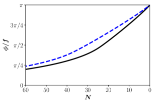
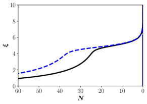
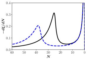
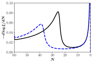
Figure 1: Evolution of the inflaton field $\phi$ and the instability parameter $\xi$ as a function of the number of $e$-folds $N$, for fiducial values $\Lambda=4.6\times 10^{-3}~{}M_{P}$, $f/M=1.7\times 10^{5}$, $\alpha=150$ (black solid lines), and $\Lambda=5.1\times 10^{-3}~{}M_{P}$, $f/M=1.5\times 10^{5}$, $\alpha=200$ (blue dashed lines), assuming always ${\cal N}=20$ fields. Additionally, we display the derivative and the logarithmic derivative of $\xi$.

Taking into account the above relations and assuming $i)$ the absence of trans-Planckian masses, $f\ll M_{P}$, $ii)$ a weak coupling regime in the inflaton-gauge interactions, $f\gg M$, $iii)$ sub-Planckian curvatures, $H\ll M_{P}$, and $iv)$ a large gravitational friction at early times $H(N_{*})\gg M$, the scalar power spectrum (3.10) can be approximated as

$$\bar{P}_{\zeta}(N)\simeq\begin{cases}\frac{4}{3\pi^{2}}\left(\frac{f}{M}\right)^{2}\left(\frac{\Lambda}{M_{P}}\right)^{8}\left(\frac{f}{\phi}\right)^{2}&\qquad\text{ for }\,\,\,\,N_{*}\geq N\gg N_{c}\,,\\[8.0pt] \frac{5\times 10^{-2}}{{\cal N}\xi^{2}}&\qquad\text{ for }\,\,\,\,N_{c}\gg N\geq 0\,,\end{cases}$$ (3.14)

with the first and second lines corresponding respectively to the strong friction [30, 76] and the strong axial regime [31, 78, 32, 42, 77].

3.2 Tensor power spectrum

The creation of gauge fluctuations via the Chern-Simons interaction $\phi\,\tilde{F}\,F$ sources also the production of helical GW. To determine their amount and chirality, let us consider the perturbed metric $d{s}^{2}={a}^{2}({\tau})\left[-d{\tau}^{2}+(\delta_{ij}+{h}_{ij})\,d{x}_{i}d{x}_{j}\right]$ with $h_{ij}$ a transverse-traceless perturbation, $h^{i}_{i}=\partial^{j}h_{ij}=0$. The variation of the quadratic expansion of the action (2.1) in $h_{ij}$ [30],

$$S_{t}^{(2)}=\frac{M_{P}^{2}}{8}\int d^{3}x\,d\tau\,a^{2}\left[\left(1-\frac{1}{2a^{2}}\frac{{\phi^{\prime}}^{2}}{M^{2}\,M_{P}^{2}}\right)h_{ij}^{\prime 2}-\left(1+\frac{1}{2a^{2}}\frac{{\phi^{\prime}}^{2}}{M^{2}\,M_{P}^{2}}\right)(\nabla{h}_{ij})^{2}\right],$$ (3.15)

leads to the following equation of motion for the tensor modes in Fourier space,

$$h^{\prime\prime}_{ij}+\left[2\frac{a^{\prime}}{a}+\frac{\beta^{\prime}}{\beta}\right]h^{\prime}_{ij}+c^{2}_{t}\,k^{2}\,h_{ij}=\frac{2}{\beta\,M^{2}_{P}}\,T_{ij}^{\text{EM}},$$ (3.16)

with

$$\beta\equiv 1-\frac{1}{2}\epsilon_{K}\,,\hskip 56.9055ptc^{2}_{t}\equiv\frac{1+\frac{1}{2}\epsilon_{K}}{1-\frac{1}{2}\epsilon_{K}}\,.$$ (3.17)

Projecting into the helicity basis defined by the polarization vectors $\epsilon^{i}_{\lambda}(\vec{k})$ and using the relations

$$h^{ij}(\tau,\,\vec{k})=\sqrt{2}\sum_{\lambda=\pm}\epsilon^{i}_{\lambda}(\vec{k})\,\epsilon^{j}_{\lambda}(\vec{k})\,h_{\lambda}(\tau,\,\vec{k})\,,\hskip 42.67912pth_{\lambda}(\tau,\,\vec{k})=\Pi_{\lambda}^{lm}h_{lm}(\tau,\,\vec{k})\,,$$ (3.18)

$$\Pi_{\lambda}^{lm}=\frac{1}{\sqrt{2}}\epsilon_{-\lambda}^{l}(\vec{k})\epsilon_{-\lambda}^{m}(\vec{k})\,,$$ (3.19)

the equation for the tensor modes with right- ($\lambda=+2$) and $(\lambda=-2$) left-handed polarizations can be written as

$$h^{\prime\prime}_{\lambda}+\left[2\frac{a^{\prime}}{a}+\frac{\beta^{\prime}}{\beta}\right]h^{\prime}_{\lambda}+c^{2}_{t}\,k^{2}\,h_{\lambda}=\frac{2}{\beta\,M^{2}_{P}}\,\Pi_{\lambda}^{lm}\,T_{lm}^{\text{EM}},$$ (3.20)

with $T^{\text{EM}}$ the energy momentum tensor for the source part of the action (2.1). Due to the projector $\Pi_{\lambda}^{lm}$, only the transverse part of this quantity contributes to the tensor perturbation, namely $T_{ij}^{\text{EM, TT}}=-a^{2}(E_{i}^{a}E_{j}^{a}+B_{i}^{a}B_{j}^{a})$. In a slow-roll quasi-de Sitter regime where both $\xi$ and $H$ are approximately constant, we can rewrite Eq. (3.20) as

$$h^{\prime\prime}_{\lambda}-\frac{2}{\tau}h^{\prime}_{\lambda}+c_{t}^{2}\,k^{2}\,\,h_{\lambda}=\frac{2}{\beta\,M^{2}_{P}}\Pi_{\lambda}^{lm}\,T_{lm}^{\text{EM}}\,,$$ (3.21)

which is formally equivalent to that in Refs. [78, 77] upon the trivial replacement $1/M_{P}^{2}\to 1/(\beta M_{P}^{2})$. Assuming again the vacuum and sourced modes to be statistically independent [36], $\left\langle h_{\lambda}(k)\,h_{\lambda}(k^{\prime})\right\rangle=\langle h_{\lambda}^{(0)}(k)\,h_{\lambda}^{(0)}(k^{\prime})\rangle+\langle h_{\lambda}^{({\rm s})}(k)\,h_{\lambda}^{({\rm s})}(k^{\prime})\rangle$, the total tensor spectrum for each polarization mode can be written as ${P}_{t,\lambda}\equiv{P}^{(0)}_{t,\lambda}+{P}^{(\rm s)}_{t,\lambda}$ with

$$P^{(0)}_{t,\lambda}=\frac{k^{3}}{2\pi^{2}}|h_{\lambda}|^{2}\simeq\frac{H^{2}}{\pi^{2}\,M_{P}^{2}\,c_{t}\,\left(1+\frac{1}{2}\epsilon_{K}\right)}\,,\hskip 42.67912ptP^{({}\rm s)}_{t,\lambda}\simeq\frac{{\cal A}_{\lambda}\,{\cal N}}{\pi^{2}\,\beta^{2}}\frac{H^{4}}{M_{P}^{4}}\frac{e^{4\pi\xi}}{\xi^{6}}\,,$$ (3.22)

the vacuum and sourced contributions, ${\cal A}_{+}\simeq 8.6\times 10^{-7}$ and ${\cal A}_{-}\simeq 1.8\times 10^{-9}$ [78]. Using these expressions, we can define the tensor-to-scalar ratio $r$ and the chirality parameter or degree of polarization $\Delta\chi$,

$$r\equiv\frac{\sum_{\lambda}P_{t,\lambda}}{{P}_{\zeta}}\,,\hskip 56.9055pt\Delta\chi\equiv\frac{P_{t,+}-P_{t,-}}{P_{t,+}+P_{t,-}}\,.$$ (3.23)

As for the scalar perturbations, we can distinguish two regimes. At early times, the friction due to the non-minimal coupling controls the dynamics, such that the contribution of the axial coupling to the tensor power spectrum is completely negligible. In this stage, the spectrum is approximately flat and non-chiral,

$$P_{t,\lambda}\simeq\frac{2}{3\pi^{2}}\left(\frac{\Lambda}{M_{P}}\right)^{4}\,,\hskip 28.45274ptr\simeq\left(\frac{M}{f}\right)^{2}\left(\frac{M_{P}}{\Lambda}\right)^{4}\left(\frac{\phi}{f}\right)^{2}\,,\hskip 28.45274pt\Delta\chi\simeq 0\,.$$ (3.24)

At later times, the exponential amplification of the $A_{+}$ modes as the field velocity increases makes them the dominant source of tensor perturbations [78, 32, 42, 77], providing an enhanced parity-violating GW background with

$$P_{t,\lambda}\simeq\frac{4\mathcal{A}_{\lambda}\mathcal{N}}{9\pi^{2}\beta^{2}}\left(\frac{\Lambda}{M_{P}}\right)^{8}{\frac{e^{4\pi\xi}}{\xi^{6}}\simeq\frac{9\mathcal{A}_{\lambda}}{\pi^{2}\mathcal{N}I_{3}^{2}\alpha^{2}\beta^{2}}\xi^{2}},\,\hskip 14.22636ptr\simeq 2.9\times 10^{2}\,\frac{\xi^{4}}{\alpha^{2}}\,,\hskip 14.22636pt\Delta\chi\simeq\frac{\delta\chi}{1+\delta\chi}\,,$$ (3.25)

where we have again assumed the strong axial regime approximation to be valid [ $H^{2}\simeq V/(3M_{P}^{2})$ and $V_{\phi}\simeq-V/f\simeq-\frac{I_{3}\,{\cal N}\,\alpha}{f}\left(H/\xi\right)^{4}e^{2\pi\xi}$ ] and defined

$$\delta\chi\equiv\frac{{\cal N}{\cal A}_{+}}{3}\left(\frac{\Lambda}{M_{P}}\right)^{4}\frac{e^{4\pi\,\xi}}{\xi^{6}}{\simeq\frac{27{\cal A}_{+}M_{p}^{4}\xi^{2}}{2I_{3}^{2}{\cal N}\alpha^{2}\beta^{2}}}\,.$$ (3.26)

4 Phenomenology

In order to assess the testability of our scenario and determine the viable parameter space, we confront now the scalar and tensor power spectra obtained in Section 3 with present and future data sets. On the one hand, we will enforce the compatibility of our predictions with current CMB observations. On the other hand, we will consider small-scale restrictions coming from PBH formation. Finally, we discuss the potential detection of chiral GW by future GW experiments.

4.1 Cosmic microwave background

The precise measurements of CMB anisotropies [2] impose strong constraints on the primordial power spectrum at scales $0.008~{}{\rm Mpc}^{-1}\lesssim k\lesssim 0.1~{}{\rm Mpc}^{-1}$, providing exquisite information on the first 7 $e$-folds of inflation. This range of knowledge is extended to about 20 $e$-folds by measurements of Lyman-$\alpha$ forest and $\mu$ spectral distortions, which are sensitive to the integrated scalar power spectrum in the range $50~{}{\rm Mpc}^{-1}\lesssim k\lesssim 10^{4}~{}{\rm Mpc}^{-1}$ [79].

The parameter space compatible with the latest Planck results on the amplitude and tilt of primordial density fluctuations [2] is displayed in the left panel of Fig. 2 for $N_{*}=60$ and ${\cal N}=20$ (cf. Section 4.2). Note that the allowed region could be additionally constrained by the kinematic restriction (B.3) in Appendix B. For the ${\cal O}(1)$ values of $\xi$ in this regime, this restriction is very mild, $\alpha\gtrsim 7.5$.

For illustration purposes, we display also exemplary power spectra in the right panel of Fig. 2. The initial values $\phi_{*}$ and $\dot{\phi}_{*}$ for the inflaton field and its derivative were fixed using its equation of motion (2.5) and the COBE normalization. Additionally, the parameters $\Lambda$ and $f/M$ are related by the spectral tilt

$$n_{s}-1\equiv\frac{d\ln P_{\zeta}(k)}{d\ln k}\simeq-2\,{\cal B}$$ (4.1)

around $N_{*}=60$. In this region, the power spectrum is fairly Gaussian since the dominant gravitationally-enhanced friction in Eq. (2.5) could be easily transferred to the axion potential (2.2) by performing a suitable field redefinition [30]. This reduces the scenario to the standard one with no extra scales and slow-roll suppressed non-Gaussianities [80]. Note that this argument does not apply to the upward bent of the spectrum at small scales, where non-Gaussianity plays indeed a very important role [44], as we now proceed to discuss.

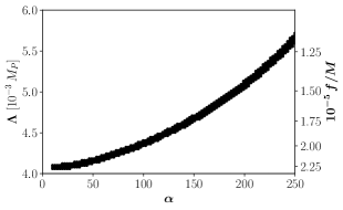
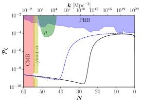
Figure 2: Left panel: Parameter space compatible with Planck results on the amplitude and tilt of primordial density fluctuations, assuming $N_{*}=60$ and ${\cal N}=20$. Right panel: Scalar spectra for the benchmark points used in Fig. 1. The colored regions are excluded by CMB anisotropies (red) [2], Lyman-$\alpha$ forest (yellow) [81], $\mu$ distortions (green) [82, 83] and PBH bounds (blue) [83, 84].

4.2 Primordial black holes

The axial enhancement of the primordial power spectrum at sub-CMB scales (cf. right panel of Fig. 2) can lead to the formation of PBH with masses of the order of the horizon mass at the time of reentry [43, 56, 85]. Assuming radiation domination to start immediately after the end of inflation and disregarding any mass growth due to merging or accretion, we have [86, 43, 56]

$$M_{\text{PBH}}(N)\simeq 4\pi\gamma\,M_{P}\,\left(\frac{M_{P}}{H}\right)\left(\frac{H_{\rm end}}{H}\right)\,e^{2N}\simeq 55\,\textrm{g}\,\gamma\,\left(\frac{10^{-6}M_{P}}{H}\right)\left(\frac{H_{\rm end}}{H}\right)\,e^{2N},$$ (4.2)

with $H=H(N)$ and $\gamma\simeq 0.4$ a parameter encoding the efficiency of the gravitational collapse [87, 88]. While PBH with masses below $10^{11}$ g decay before big bang nucleosynthesis, heavier black holes can play the role of dark matter and are severely constrained by direct searches [83, 89]. These bounds restrict the primordial power spectrum on scales much smaller than those currently probed by CMB and large scale structure surveys, providing an invaluable information on the last 40 $e$-folds of inflation.

The formation of a PBH is a rare event. For a given perturbation amplitude in the scalar power spectrum, the fraction of causal regions collapsing into PBH is given by

$$\beta=\int_{\zeta_{c}}^{\infty}{\cal P}\left(\zeta_{k}\right)\,d\zeta_{k}\,,$$ (4.3)

with ${\cal P}\left(\zeta_{k}\right)$ the probability density of perturbations and $\zeta_{c}\sim 0.5$ a critical threshold [87, 91], within the range $\zeta_{c}\sim{\cal O}(0.05-1)$ [92, 91, 85] suggested by the analytic and numerical studies in Refs. [93, 88]. As shown in Section 3.1, the enhanced part of the power spectrum (3.10) can be well-approximated by its axial contribution (3.14), which is generated by the convolution of two Gaussian modes ($A+A\to\delta\phi$) and obeys therefore a $\chi^{2}$ statistics [43]. For this distribution, Eq. (4.3) becomes

$$\beta_{\chi^{2}}(N)={\rm Erfc}\left(\sqrt{\frac{1}{2}+\frac{\zeta_{c}}{\sqrt{2P_{\zeta}(N)}}}\right)\;,$$ (4.4)

with ${\rm Erfc}\left(x\right)\equiv 1-{\rm Erf}\left(x\right)$ the complementary error function. Together with Eq. (4.2), this expression allows to convert the primordial power spectrum $\bar{P}_{\zeta}$ into a limit on the PBH abundance and vice versa. We follow here the second approach and display in the right panel of Fig. 2 the restrictions on the power spectrum following from present PBH bounds [83]. The minimal number of fields needed to pass these constraints turns out to very moderate (${\cal N}\simeq 20$) and can be easily accommodated in usual grand unified groups such as $SU(N)$ without significantly altering the treatment presented here.

The above analysis is just meant to illustrate the versatility of our scenario and should be not be understood as a precise one. For the sake of clarity, there are several subtleties that should be mentioned here:

1. Slow-roll validity. It is a well-established fact that the production of PBHs in single-field scenarios driven by a potential requires the existence of an inflection point along the inflationary trajectory where the slow-roll conditions are severely violated [94, 95]. We emphasize that this important result, usually stated as a no-go theorem, does not directly apply to the problem at hand. In particular, the enhancement of the primordial power spectrum at small scales is not related to any special feature of the potential but rather to the explosive production of gauge fluctuations which subsequently source curvature perturbations. The validity of the slow-roll approximation during the whole inflationary evolution is illustrated in the lower panel of Fig. 3, where we display the result of numerically solving the system of equations (2.3), (2.4) and (2.5).

   

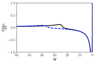
   Figure 3: Evolution of the derivative of the slow-roll parameter $\epsilon=-\dot{H}/H^{2}$ as a function of the number of $e$-folds $N$, for the benchmark points used in Fig. 1.

2. Critical threshold. We followed closely the approach of Refs. [92, 91, 85], employing a critical threshold $\zeta_{c}\sim 0.5$. A precise calculation should take into account, however, the full shape of the correlation functions since $\zeta_{c}$ depends strongly on the real space distribution of overdensities [96, 97, 98, 99], being lower for broader shapes where pressure gradients play are less important role.

3. Non-Gaussianities. The formation of PBHs is inevitably a non-Gaussian process [100, 101] and the precise calculation of the abundance should involve a priori the convolution of two non-Gaussian modes instead of two Gaussian ones.

4. Post-inflationary evolution. We are implicitly assuming a standard $\Lambda$CDM scenario where gravity is the only attractive force for the clumping of matter. Alternative cosmologies involving fifth forces and/or deviations from radiation domination during the earliest post-inflationary epochs [84] could affect the above estimates, allowing even for the formation of PBHs without the need of a significant enhancement of the primordial power spectrum of density fluctuations [102, 103, 104].

A precise and self-consistent computation should take into account the aforementioned details while involving a combination of numerical and analytical approaches, as done for instance in Refs. [97, 105, 106] for standard $\Lambda$CDM scenarios. However, it is not in the scope of this work to go beyond the approximation implied by the $\chi^{2}$ statistics (4.4) [92, 91] and the choice of a particular threshold $\zeta_{c}$, since the potential changes on the restrictions on the shape and amplitude of the primordial power spectrum are expected to be degenerate with the model parameters controlling the transition time $N_{c}$ in Eq. (3.12) and the number of fields ${\cal N}$, respectively. A more complete and detailed discussion is left for a future research work.

4.3 Gravitational waves

Gravitational waves are probably the most promising relic to probe the unknown early Universe. Interestingly, the late-time amplification of the inflationary power-spectrum in the strong axial regime opens the possibility of obtaining an observable chiral GW signal in the frequency range probed by future terrestrial and space interferometers. The associated fractional energy density per logarithmic frequency interval $f_{\rm GW}=k/2\pi$ is given by [37]

$$\Omega_{\rm GW}\equiv\frac{1}{\rho_{c}}\,\frac{\partial\rho_{\rm GW,0}}{\partial\log\,k}=\frac{\Omega_{\rm R,0}}{24}\sum_{\lambda}P_{t,\lambda}\,,$$ (4.5)

with $\Omega_{{\rm R},0}\,h^{2}\simeq 4.2\times 10^{-5}$ the radiation density parameter today, $P_{t,\lambda}$ the GW power spectra in Eq. (3.22) and

$$N=N_{*}-44.92+{\rm ln}\left(\frac{k_{*}}{0.002\,{\rm Mpc}^{-1}}\right)-{\rm ln}\left(\frac{f_{\rm GW}}{100\,{\rm Hz}}\right)+{\rm ln}\left(\frac{H_{N}}{H_{*}}\right)\,,$$ (4.6)

with $N_{*}=60$ and $H_{N}$ the value of the Hubble rate $N$ $e$-folds before the end of inflation.

The frequency dependence in Eq. (4.5) takes the schematic form $\Omega_{\rm GW}h^{2}\simeq f_{\rm GW}^{n_{t}}$, with

$$n_{t}(f_{\rm GW})=\frac{d\ln\Omega_{\rm GW}h^{2}}{d\ln f_{\rm GW}}$$ (4.7)

the tensor spectral tilt, understood as a time-dependent quantity. During the first stages of the evolution $(N_{*}\geq N\gg N_{c})$ the tensor power spectrum is dominated by the vacuum contribution in Eq. (3.22). In this regime, and at the leading order in the slow-roll parameters $\epsilon_{H}=-\dot{H}/H^{2}$ and $\eta\equiv-\ddot{\phi}/(H\dot{\phi})$, we have

$$n_{t}(f_{\rm GW})\simeq-2\epsilon_{H}=-\left(\frac{M}{f}\right)^{2}\left(\frac{M_{P}}{\Lambda}\right)^{4}\,,$$ (4.8)

up to mild corrections associated with the field evolution displayed in Fig. 1. On the other hand, the tensor spectral tilt at late times ($N\ll N_{c}$) is rather given by [107],

$$n_{t}(f_{\rm GW})=-4\epsilon_{H}+4\pi\frac{d\xi}{dN}-6\frac{d\ln\xi}{dN}\,.$$ (4.9)

Since the backreaction of the gauge fields on the Hubble rate is small almost till the end of inflation (cf. Appendix B), we can still approximate the slow-roll parameter $\epsilon_{H}$ by its value in Eq. (4.8) during this regime, i.e. assume inflation to be still driven by the potential. On the other hand, from Fig. 1 we can infer that a good approximation to the $\xi$ evolution during this stage is $\xi=aN+b$. In the absence of a simple analytical solution, these coefficients have to be extracted by fitting the numerical solution for $\xi$. However, as can be seen from Fig. 4, the power-law approximation provides a reasonably good fit to the slope of the GW spectrum.

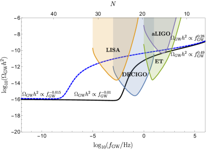
Figure 4: GW spectra for the benchmark points used in Fig. 1. The asymptotic power law behavior is obtained from the analytical approximations in Eq. (4.7). The experimental power-law integrated sensitivity curves account for the enhancement in detector sensitivity following the integration over frequency on top of the integration over time [108, 109].

The GW spectra generated by our mechanism for the benchmark points in Figs. 1 and 2 are compared in Fig. 4 with the power-law integrated sensitivity curves of different experiments. The Laser Interferometer Space Antenna (LISA) [110] is mostly sensitive to frequencies $10^{-4}\lesssim f\lesssim 10^{-1}$ Hz, corresponding to momenta $10^{11}\,{\rm Mpc}^{-1}\lesssim k\lesssim 10^{14}\,{\rm Mpc}^{-1}$ or an $e$-fold range $22\lesssim N\lesssim 28$. The Deci-hertz Interferometer Gravitational wave Observatory (DECIGO) [111, 112], the advanced LIGO detector (aLIGO) [113] and the Einstein Telescope (ET) [114] extend this range all the way up to $\sim 10^{2}-10^{3}$ Hz, corresponding to scales around $k\sim 10^{17}-10^{18}\,{\rm Mpc}^{-1}$ and $N\sim 15$. Note that, although our GW spectra display generically a “knee” rather than a peak structure, they are maximally chiral and non-Gaussian, which could serve as a smoking gun for this mechanism and facilitate their discrimination against astrophysical backgrounds (see e.g. Refs. [115, 116, 117, 118]). Although the measurement of the polarization is more challenging than the measure of the total spectrum, there are good prospects of detection with future experiments such as LISA or ET for sufficiently large amplitude of the total spectrum [119, 120].

Overall, the synergy of shift-symmetric interactions advocated in this paper reconciles Natural Inflation scenarios with well-motivated UV expectations, while providing a rich phenomenology over a humongous range of scales. The natural enhancement of scalar and tensor perturbations taking place at the end of inflation translates into the simultaneous production of a dark matter component in the form of PBH and a chiral GW signal within the reach of future GW interferometers, opening the possibility of testing the model with sub-CMB physics. Our estimates rely, of course, on the accuracy of Eqs. (2.15) and (3.5), meaning that ${\cal O}(1)$ corrections should be certainly expected, especially in the large $\xi$ regime. A fully numerical computation along the lines of Refs. [121, 122, 123, 124, 125, 126] will most likely be required to obtain precise results. Having presented the main qualitative features of our scenario, we postpone this detailed study to a future publication.

Appendix A Action for scalar perturbations

In this Appendix, we present a detailed derivation of the total spectrum of primordial density fluctuations in Eqs. (3.6) and (3.7). Following the standard Arnowitt-Deser-Misner (ADM) approach [127], we consider the metric decomposition

$${\rm d}s^{2}=-N^{2}\,{\rm d}t^{2}+\gamma_{ij}\,\left({\rm d}x^{i}+\beta^{i}{\rm d}t\right)\,\left({\rm d}x^{j}+\beta^{j}{\rm d}t\right),$$ (A.1)

together with the gauge choice $N=1+n\,;\beta_{i}=\partial_{i}\psi\,;\gamma_{ij}=a^{2}(t)\,\delta_{ij}\,;\phi(x^{i},\,t)=\phi_{0}(t)+\delta\phi(x^{i},\,t)\,,$ with $\phi_{0}(t)$ the homogeneous background component of the inflaton field. After expanding up to second order and integrating by parts, the scalar part of the action (2.1) is rewritten as [73]

$$S^{(2)}_{\delta\phi}=\int{\rm d}^{4}x\,a^{3}\frac{F^{2}\,G}{\epsilon_{K}}\left[\delta\dot{\phi}^{2}-\frac{c_{s}^{2}}{a^{2}}\,(\nabla\delta\phi)^{2}-m^{2}\,\delta\phi^{2}\right]+\int{\rm d}^{4}x\,a^{3}\,\frac{\alpha}{f}\,\delta[\vec{E}_{a}\cdot\vec{B}_{a}]\delta\phi\,.$$ (A.2)

Here the equations for $\psi$ and $n$ are solved in terms of $\delta\phi$ and plugged back in the quadratic action. By doing that, one obtains the effective speed of sound $c_{s}$ and mass $m$, namely

$$c_{s}^{2}=\frac{\epsilon_{K}}{2\left(1-\frac{1}{2}\epsilon_{K}\right)G}\left[\left(1+\frac{3}{2}\epsilon_{K}\right)K+\frac{2H^{2}\epsilon_{K}}{M^{2}F}+6\frac{\dot{H}}{M^{2}}\left(1-\frac{1}{2}\epsilon_{K}\right)\right]\,,$$ (A.3)

$$m^{2} \equiv \frac{\epsilon_{K}}{2G\,F^{2}}\left[V_{\phi\phi}\,F+\frac{V_{\phi}}{M_{P}}\frac{M}{H}\frac{\sqrt{\epsilon_{K}}}{1-\frac{3}{2}\epsilon_{K}}\left(K+3\frac{H^{2}}{M^{2}}+\frac{1+\frac{3}{2}\epsilon_{K}}{1-\frac{3}{2}\epsilon_{K}}\left(\frac{1}{2}K+\dot{H}\frac{1-\frac{1}{2}\epsilon_{K}}{M^{2}\epsilon_{K}}\right)\right)\right.$$

$$-\left.\frac{K^{2}M^{2}\epsilon_{K}(M^{2}\epsilon_{K}+6H^{2}(3\epsilon_{K}-1))}{4H^{2}(1-\frac{3}{2}\epsilon_{K})^{2}}-\frac{1}{a^{3}}\frac{{\rm d}}{{\rm d}t}\left(\frac{a^{3}KM^{2}\epsilon_{K}\left(K+\frac{\epsilon_{K}}{2}\left(\frac{9H^{2}}{M^{2}}-1\right)\right)}{2H(1-\frac{3}{2}\epsilon_{K})^{2}}\right)\right],$$

where $K$, $\epsilon_{K}$, $F$ and $G$ are defined in Eqs. (2.6) and (3.3), and $\delta[\vec{E}_{a}\cdot\vec{B}_{a}]$ includes the first-order perturbations of the axial term $\phi\,F\,\tilde{F}$, cf. Eq. (3.4). Introducing the canonical Mukhanov-Sasaki variables (3.2), integrating by parts and performing some algebraic manipulations, the action (A.2) can be reduced to the form (3.1). The solution of the associated equations of motion in Fourier space is given by the sum of a vacuum homogeneous solution $u^{(0)}$ including the effect of the non-minimal kinetic coupling and a particular solution $u^{(\rm{s})}$ sourced by the axial coupling, i.e. $u(k,\,\tau)=u^{(0)}(k,\,\tau)+u^{(\rm{s})}(k,\,\tau)$.

The spectrum of vacuum scalar perturbations $u^{(0)}(k)$ is computed by solving the homogeneous part of Eq. (3.5). To this end, we work within the approximation in which the perturbations’ speed of sound $c_{s}$ is constant and assume a nearly de Sitter background $a\simeq-(H\,\tau(1-\epsilon_{H}))^{-1}$, with $\epsilon_{H}=-\dot{H}/H^{2}$. With this, we obtain

$$\frac{z^{\prime\prime}}{z}\simeq\frac{2}{\tau^{2}}\left[1+\frac{3}{2}\epsilon_{H}+\delta_{K}\right]+{\cal O}(\epsilon_{H}^{2})\,,$$ (A.5)

with $\delta_{K}$ defined in Eq. (3.9), and $z\simeq a\sqrt{K}$. Therefore, the homogeneous part of Eq. (3.5) becomes

$$u^{(0)}{{}^{\prime\prime}}+\left[c_{s}^{2}\,k^{2}-\frac{1}{\tau^{2}}\left(\nu^{2}-\frac{1}{4}\right)\right]u^{(0)}=0\,,$$ (A.6)

with $\nu$ given in Eq. (3.9). The solution that matches the Bunch-Davies vacuum initial condition $\lim_{\tau\rightarrow-\infty}u(k,\,\tau)=e^{-i\,c_{s}\,k\,\tau}/\sqrt{2c_{s}\,k}$ is given by

$$u^{(0)}=\sqrt{\frac{\pi}{2}}\frac{e^{i\frac{\pi}{2}(\nu+\frac{1}{2})}}{\sqrt{2c_{s}\,k}}\sqrt{-c_{s}\,k\,\tau}\,H^{(1)}_{\nu}(-c_{s}\,k\,\tau)\,,$$ (A.7)

with $H_{\nu}^{(1)}$ the Hankel function of the first kind. The super-horizon limit of this solution

$$\lim_{|c_{s}k\tau|\rightarrow 0}u^{(0)}(k)=\frac{2^{\nu-3/2}\,e^{i\frac{\pi}{2}(\nu-1/2)}}{\sqrt{2c_{s}\,k}}\,\frac{\Gamma(\nu)}{\Gamma(3/2)}\,\left(-c_{s}\,k\,\tau\right)^{1/2-\nu}$$ (A.8)

allows to compute the spectrum of the vacuum primordial curvature perturbations $\zeta=-H\delta\phi/\dot{\phi}_{0}=-H\,u/(z\,\dot{\phi}_{0})$, namely

$$\delta(\vec{k}+\vec{k}^{\prime})\,P^{(0)}_{\zeta}(k)=\frac{k^{3}}{2\pi^{2}}\frac{H^{2}}{\dot{\phi}_{0}^{2}}\langle\delta\phi^{(0)}(\vec{k})\,\delta\phi^{(0)}(\vec{k}^{\prime})\rangle=\frac{k^{3}}{2\pi^{2}}\frac{H^{2}}{z^{2}\dot{\phi}_{0}^{2}}\langle u^{(0)}(\vec{k})\,u^{(0)}(\vec{k}^{\prime})\rangle\,,$$ (A.9)

which, in a de Sitter background, becomes

$$P^{(0)}_{\zeta}(k)=\frac{k^{3}}{\pi^{2}}\frac{H^{2}}{z^{2}\,\dot{\phi}_{0}^{2}}\frac{2^{2\nu-5}}{c_{s}\,k}\left|\frac{\Gamma(\nu)}{\Gamma(\frac{3}{2})}\right|^{2}\left(-c_{s}\,k\,\tau\right)^{1-2\nu}\simeq\frac{H^{4}}{8\pi^{2}\dot{\phi}_{0}^{2}}\frac{\epsilon_{K}}{F^{2}\,G\,c_{s}^{3}}\left|\frac{\Gamma(\nu)}{\Gamma(\frac{3}{2})}\right|^{2}\left(\frac{-c_{s}\,k\,\tau}{2}\right)^{3-2\nu}.$$ (A.10)

In an analogous way, we can compute the spectrum of the perturbations sourced by the axial coupling, i.e. $u^{(\rm s)}(k)$. Starting again with Eq. (3.5) in a nearly de Sitter background, we can write

$$u^{({\rm s})}{{}^{\prime\prime}}+\left[c_{s}^{2}\,k^{2}-\frac{1}{\tau^{2}}\left(\nu^{2}-\frac{1}{4}\right)\right]u^{(\rm{s})}=\frac{\alpha}{f}\,\frac{a^{4}}{z}\,\delta[\vec{E}_{a}\cdot\vec{B}_{a}]\,,$$ (A.11)

with $\delta[{\vec{E}_{a}}\cdot{\vec{B}_{a}}]\simeq\delta_{{\vec{E}_{a}}\cdot{\vec{B}_{a}}}+(\partial\langle\vec{E}_{a}\cdot\vec{B}_{a}\rangle/\partial\dot{\phi})\delta\dot{\phi}$. Following Ref. [31], we evaluate the variation of $\langle\vec{E}_{a}\cdot\vec{B}_{a}\rangle$ as

$$\frac{\partial\langle\vec{E}_{a}\cdot\vec{B}_{a}\rangle}{\partial\dot{\phi}}\delta\dot{\phi}\simeq\frac{\partial\langle\vec{E}_{a}\cdot\vec{B}_{a}\rangle}{\partial\xi}\frac{\partial\xi}{\partial\dot{\phi}}\delta\dot{\phi}\simeq\frac{\partial\langle\vec{E}_{a}\cdot\vec{B}_{a}\rangle}{\partial\xi}\frac{\alpha}{2fH}\delta\dot{\phi}\simeq\frac{\pi\alpha}{f}\langle\vec{E}_{a}\cdot\vec{B}_{a}\rangle\frac{\delta\phi^{\prime}}{aH}\,.$$ (A.12)

In the strong axial regime, we can approximate $V_{\phi}\simeq(\alpha/f)\langle\vec{E}_{a}\cdot\vec{B}_{a}\rangle$ and write the variation of the source term as $\delta[{\vec{E}_{a}}\cdot{\vec{B}_{a}}]\simeq\delta_{{\vec{E}_{a}}\cdot{\vec{B}_{a}}}+\pi V_{\phi}\delta\phi^{\prime}/(aH)$. Taking into account that $u=z\,\delta\phi$, and neglecting the subdominant gradient term at super horizon scales, Eq. (A.11) becomes

$$u^{({\rm s})}{{}^{\prime\prime}}+\frac{\sigma}{\tau}\,u^{({\rm s})}{{}^{\prime}}-\frac{1}{\tau^{2}}\left(\nu^{2}-\frac{1}{4}-\sigma\right)u^{(\rm{s})}=\frac{\alpha}{f}\,\frac{a^{4}}{z}\,\delta_{{\vec{E}_{a}}\cdot{\vec{B}_{a}}}\,,$$ (A.13)

with $\sigma$ given in Eq. (3.8). Using now Eq. (2.12) and taking into account that $u^{(\rm{s})}\simeq a\,\sqrt{K}\,\delta\phi^{(\rm s)}$, we obtain [31, 77]

$$\langle\delta\phi^{(\rm s)}(\vec{k})\,\delta\phi^{(\rm s)}(\vec{k}\,^{\prime})\rangle \simeq \frac{{\cal F}\,H^{4}}{{\cal N}}\frac{\delta(\vec{k}+\vec{k}\,^{\prime})}{k^{3}}\left(\frac{\alpha\,{\cal N}}{\Delta\,K\,f}\right)^{2}\,\frac{e^{4\pi\xi}}{\xi^{8}}{(-2^{5}\xi\,k\,\tau)^{2+2\nu_{\pm}}},$$ (A.14)

with ${\cal F}\simeq 2.13\times 10^{-6}$, $\Delta$ given in Eq. (3.8) and the indices $\nu_{\pm}\equiv\frac{1}{2}\left(1-\sigma\pm\Delta\right)$ corresponding to the growing and decaying solutions of Eq. (A.13). The $1/{\cal N}$ factor in this expression comes from assuming that the contributions of the ${\cal N}$ gauge fields to the two-point function of $\delta_{\vec{E}_{a}\cdot\vec{B}_{a}}$ add incoherently [31, 32]. Using this result, the sourced contribution to the spectrum of the primordial curvature perturbations $\zeta^{(\rm s)}=-H\,\delta\phi^{(\rm s)}/\dot{\phi}_{0}$,

$$\delta(\vec{k}+\vec{k}\,^{\prime})\,P^{(\rm s)}_{\zeta}(k)\equiv\frac{k^{3}}{2\pi^{2}}\,\frac{H^{2}}{\dot{\phi}_{0}^{2}}\,\langle\delta\phi^{(\rm s)}(\vec{k})\,\delta\phi^{(\rm s)}(\vec{k}\,^{\prime})\rangle\,,$$ (A.15)

becomes

$$P^{(\rm s)}_{\zeta}(k)\simeq\frac{\,H^{4}}{4\pi^{2}\dot{\phi}_{0}^{2}}\left[\frac{2{\cal F}}{{\cal N}}\left(\frac{\alpha\,{{\cal N}}\,H}{\Delta\,K\,f}\right)^{2}\,\frac{e^{4\pi\xi}}{\xi^{8}}{(-2^{5}\xi\,k\,\tau)^{2+2\nu_{\pm}}}\right]\,.$$ (A.16)

Combining this result with the vacuum contribution (A.10), we obtain the total spectrum of primordial density fluctuations in Eqs. (3.6) and (3.7). These expressions are accurate up to ${\cal O}(1)$ corrections associated with the precise choice of the pivot scale $k_{*}$.

Appendix B Slow-roll regime and backreaction

In this Appendix we analyze the conditions allowing for an inflationary epoch in the presence of gauge modes production and gravitationally-induced friction. To this end, we note that the first Friedmann equation (2.3) can be written as the cosmic sum rule $\Omega_{\text{EM}}+\Omega_{\rm K}+\Omega_{\rm V}=1$, with

$$\Omega_{\text{EM}}\equiv\frac{\langle\vec{E}_{a}^{2}\rangle+\langle\vec{B}_{a}^{2}\rangle}{6M_{P}^{2}H^{2}}\,,\hskip 42.67912pt\Omega_{\rm K}\equiv\frac{\dot{\phi}^{2}}{6M^{2}_{P}H^{2}}\left(1+9\frac{H^{2}}{M^{2}}\right)\,,\hskip 42.67912pt\Omega_{\rm V}\equiv\frac{V(\phi)}{3M_{P}^{2}H^{2}}$$ (B.1)

the density parameters for the gauge fields and the inflaton kinetic and potential components. In order to have a potential-driven inflationary epoch, we need to make sure that both $\Omega_{\rm K}$ and $\Omega_{\text{EM}}$ are much smaller than the potential term $\Omega_{\rm V}$. More generically, the requirements $\Omega_{\text{EM}}\leq 1$ and $\Omega_{\rm K}\leq 1$ are consistency checks on the parameter space:

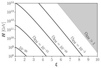
Figure 5: Level curves for the $\Omega_{\text{EM}}$ contribution to the energy density. Notice that the region above the curve corresponding to $\Omega_{\text{EM}}=1$ is forbidden as it would imply more than $100\%$ energy density stored in the gauge fields.

1. Using the relations (2.13) and (2.14), the condition $\Omega_{\text{EM}}\leq 1$ becomes

   $$\Omega_{\text{EM}}\simeq 3\times 10^{-16}\mathcal{N}\,e^{2\pi\xi}\left(\frac{2.6}{\xi^{3}}+\frac{3}{\xi^{5}}\right)\left(\frac{H}{10^{13}\,{\rm GeV}}\right)^{2}\leq 1\,,$$ (B.2)

   meaning that, as shown in Fig. 5, there exists a maximum value for the Hubble rate $H$ for each value of the instability parameter $\xi$. For instance, for $\xi=6$ and a single gauge field $\mathcal{N}=1$, we have $H\lesssim 10^{14}$ GeV. From a dynamical point of view, the growth of the instability parameter $\xi$ towards the end of inflation, increases the energy density of gauge fluctuations while dissipating the energy density of the inflaton condensate. This is a very efficient heating mechanism leading potentially to a very rapid thermalization for non-Abelian gauge sectors [128].

2. Using Eq. (2.10), the condition $\Omega_{\rm K}\leq 1$ in the strong friction limit $H\gg M$ can be written as

   $$\Omega_{\rm K}\simeq 6\left(\frac{\xi}{\alpha}\right)^{2}\left(\frac{f}{M}\right)^{2}\left(\frac{H}{M_{P}}\right)^{2}\leq 1\,.$$ (B.3)

   Numerically, and for the range of parameters considered in this paper, this translates into an approximate relation $\alpha\gtrsim 7.5\,\xi$.

For the sake of completeness, we discuss also here the interplay between the gravitationally-enhanced friction generated by the non-minimal derivative coupling to gravity and the one induced by the exponential growth of gauge fluctuations. Depending on the hierarchy of scales, any of these two independent mechanisms can a priori dominate. Here we want to determine when the contribution coming from the gauge fields becomes relevant. Assuming as usual a small acceleration in the Klein-Gordon equation (2.5), the evolution of the scalar field is approximately given by $3\,H\,K\,\dot{\phi}+V_{\phi}\simeq\frac{\alpha}{f}\langle\vec{E}_{a}\cdot\vec{B}_{a}\rangle$, where we have neglected a term proportional to $\epsilon_{H}\ll 1$. Comparing the two friction terms in this equation, we get

$$R\equiv\left|\frac{\alpha\,\langle E_{a}\cdot B_{a}\rangle}{3HK\dot{\phi}f}\right|\simeq\frac{I_{3}\,\alpha^{2}\mathcal{N}H^{2}}{6f^{2}K}\frac{e^{2\pi\xi}}{\xi^{5}}\simeq 10^{-5}{\mathcal{N}}\left(\alpha\frac{M}{f}\right)^{2}\frac{e^{2\pi\xi}}{\xi^{5}}\,,$$ (B.4)

where in the last equality we have assumed the high gravitational friction limit $H/M\gg 1$. As long as this ratio is much smaller than one, the contribution coming from the gauge fields in the Klein-Gordon equation can be safely neglected. For the parameter space compatible with Planck results on the amplitude and tilt of primordial density fluctuations, and assuming $N_{*}=60$ and ${\cal N}=20$ (left panel of Fig. 2), $R$ approaches unity when the instability parameter reaches $\xi\sim 5-6$.

References

- [1] WMAP collaboration, Nine-Year Wilkinson Microwave Anisotropy Probe (WMAP) Observations: Cosmological Parameter Results, Astrophys. J. Suppl. 208 (2013) 19 [1212.5226].
- [2] Planck collaboration, Planck 2018 results. X. Constraints on inflation, 1807.06211.
- [3] J. García-Bellido, J. Rubio, M. Shaposhnikov and D. Zenhausern, Higgs-Dilaton Cosmology: From the Early to the Late Universe, Phys. Rev. D84 (2011) 123504 [1107.2163].
- [4] F. Bezrukov, G. K. Karananas, J. Rubio and M. Shaposhnikov, Higgs-Dilaton Cosmology: an effective field theory approach, Phys. Rev. D 87 (2013) 096001 [1212.4148].
- [5] J. Rubio and M. Shaposhnikov, Higgs-Dilaton cosmology: Universality versus criticality, Phys. Rev. D 90 (2014) 027307 [1406.5182].
- [6] C. Burgess, S. P. Patil and M. Trott, On the Predictiveness of Single-Field Inflationary Models, JHEP 06 (2014) 010 [1402.1476].
- [7] F. Bezrukov, M. Pauly and J. Rubio, On the robustness of the primordial power spectrum in renormalized Higgs inflation, JCAP 02 (2018) 040 [1706.05007].
- [8] J. Rubio, Scale symmetry, the Higgs and the Cosmos, in 19th Hellenic School and Workshops on Elementary Particle Physics and Gravity, 3, 2020, 2004.00039.
- [9] B. J. Broy, M. Galante, D. Roest and A. Westphal, Pole inflation — Shift symmetry and universal corrections, JHEP 12 (2015) 149 [1507.02277].
- [10] B. Finelli, G. Goon, E. Pajer and L. Santoni, The Effective Theory of Shift-Symmetric Cosmologies, JCAP 05 (2018) 060 [1802.01580].
- [11] K. Freese, J. A. Frieman and A. V. Olinto, Natural inflation with pseudo - Nambu-Goldstone bosons, Phys. Rev. Lett. 65 (1990) 3233.
- [12] F. C. Adams, J. R. Bond, K. Freese, J. A. Frieman and A. V. Olinto, Natural inflation: Particle physics models, power law spectra for large scale structure, and constraints from COBE, Phys. Rev. D47 (1993) 426 [hep-ph/9207245].
- [13] K. Freese and W. H. Kinney, Natural Inflation: Consistency with Cosmic Microwave Background Observations of Planck and BICEP2, JCAP 03 (2015) 044 [1403.5277].
- [14] R. Peccei and H. R. Quinn, CP Conservation in the Presence of Instantons, Phys. Rev. Lett. 38 (1977) 1440.
- [15] T. Banks, M. Dine, P. J. Fox and E. Gorbatov, On the possibility of large axion decay constants, JCAP 06 (2003) 001 [hep-th/0303252].
- [16] P. Svrcek and E. Witten, Axions In String Theory, JHEP 06 (2006) 051 [hep-th/0605206].
- [17] N. Arkani-Hamed, L. Motl, A. Nicolis and C. Vafa, The String landscape, black holes and gravity as the weakest force, JHEP 06 (2007) 060 [hep-th/0601001].
- [18] M. Kawasaki, M. Yamaguchi and T. Yanagida, Natural chaotic inflation in supergravity, Phys. Rev. Lett. 85 (2000) 3572 [hep-ph/0004243].
- [19] N. Arkani-Hamed, H.-C. Cheng, P. Creminelli and L. Randall, Extra natural inflation, Phys. Rev. Lett. 90 (2003) 221302 [hep-th/0301218].
- [20] J. E. Kim, H. P. Nilles and M. Peloso, Completing natural inflation, JCAP 01 (2005) 005 [hep-ph/0409138].
- [21] S. Dimopoulos, S. Kachru, J. McGreevy and J. G. Wacker, N-flation, JCAP 08 (2008) 003 [hep-th/0507205].
- [22] T. W. Grimm, Axion inflation in type II string theory, Phys. Rev. D 77 (2008) 126007 [0710.3883].
- [23] L. McAllister, E. Silverstein and A. Westphal, Gravity Waves and Linear Inflation from Axion Monodromy, Phys. Rev. D 82 (2010) 046003 [0808.0706].
- [24] N. Kaloper and L. Sorbo, A Natural Framework for Chaotic Inflation, Phys. Rev. Lett. 102 (2009) 121301 [0811.1989].
- [25] M. Czerny and F. Takahashi, Multi-Natural Inflation, Phys. Lett. B 733 (2014) 241 [1401.5212].
- [26] K. Choi, H. Kim and S. Yun, Natural inflation with multiple sub-Planckian axions, Phys. Rev. D 90 (2014) 023545 [1404.6209].
- [27] R. Kappl, S. Krippendorf and H. P. Nilles, Aligned Natural Inflation: Monodromies of two Axions, Phys. Lett. B 737 (2014) 124 [1404.7127].
- [28] F. Carta, N. Righi, Y. Welling and A. Westphal, Harmonic Hybrid Inflation, 2007.04322.
- [29] C. Germani and A. Kehagias, UV-Protected Inflation, Phys. Rev. Lett. 106 (2011) 161302 [1012.0853].
- [30] C. Germani and Y. Watanabe, UV-protected (Natural) Inflation: Primordial Fluctuations and non-Gaussian Features, JCAP 1107 (2011) 031 [1106.0502].
- [31] M. M. Anber and L. Sorbo, Naturally inflating on steep potentials through electromagnetic dissipation, Phys. Rev. D81 (2010) 043534 [0908.4089].
- [32] M. M. Anber and L. Sorbo, Non-Gaussianities and chiral gravitational waves in natural steep inflation, Phys. Rev. D85 (2012) 123537 [1203.5849].
- [33] M. M. Anber and L. Sorbo, N-flationary magnetic fields, JCAP 0610 (2006) 018 [astro-ph/0606534].
- [34] R. Durrer, L. Hollenstein and R. K. Jain, Can slow roll inflation induce relevant helical magnetic fields?, JCAP 1103 (2011) 037 [1005.5322].
- [35] N. Barnaby and M. Peloso, Large Nongaussianity in Axion Inflation, Phys. Rev. Lett. 106 (2011) 181301 [1011.1500].
- [36] N. Barnaby, R. Namba and M. Peloso, Phenomenology of a Pseudo-Scalar Inflaton: Naturally Large Nongaussianity, JCAP 1104 (2011) 009 [1102.4333].
- [37] N. Barnaby, E. Pajer and M. Peloso, Gauge Field Production in Axion Inflation: Consequences for Monodromy, non-Gaussianity in the CMB, and Gravitational Waves at Interferometers, Phys. Rev. D85 (2012) 023525 [1110.3327].
- [38] N. Barnaby, R. Namba and M. Peloso, Observable non-gaussianity from gauge field production in slow roll inflation, and a challenging connection with magnetogenesis, Phys. Rev. D85 (2012) 123523 [1202.1469].
- [39] P. Adshead and M. Wyman, Chromo-Natural Inflation: Natural inflation on a steep potential with classical non-Abelian gauge fields, Phys. Rev. Lett. 108 (2012) 261302 [1202.2366].
- [40] K. Dimopoulos and M. Karciauskas, Parity Violating Statistical Anisotropy, JHEP 06 (2012) 040 [1203.0230].
- [41] P. D. Meerburg and E. Pajer, Observational Constraints on Gauge Field Production in Axion Inflation, JCAP 1302 (2013) 017 [1203.6076].
- [42] N. Barnaby, J. Moxon, R. Namba, M. Peloso, G. Shiu and P. Zhou, Gravity waves and non-Gaussian features from particle production in a sector gravitationally coupled to the inflaton, Phys. Rev. D86 (2012) 103508 [1206.6117].
- [43] A. Linde, S. Mooij and E. Pajer, Gauge field production in supergravity inflation: Local non-Gaussianity and primordial black holes, Phys. Rev. D87 (2013) 103506 [1212.1693].
- [44] J. L. Cook and L. Sorbo, An inflationary model with small scalar and large tensor nongaussianities, JCAP 11 (2013) 047 [1307.7077].
- [45] M. Shiraishi, A. Ricciardone and S. Saga, Parity violation in the CMB bispectrum by a rolling pseudoscalar, JCAP 1311 (2013) 051 [1308.6769].
- [46] P. Fleury, J. P. Beltrán Almeida, C. Pitrou and J.-P. Uzan, On the stability and causality of scalar-vector theories, JCAP 1411 (2014) 043 [1406.6254].
- [47] C. Caprini and L. Sorbo, Adding helicity to inflationary magnetogenesis, JCAP 1410 (2014) 056 [1407.2809].
- [48] R. Z. Ferreira and M. S. Sloth, Universal Constraints on Axions from Inflation, JHEP 12 (2014) 139 [1409.5799].
- [49] N. Bartolo, S. Matarrese, M. Peloso and M. Shiraishi, Parity-violating and anisotropic correlations in pseudoscalar inflation, JCAP 1501 (2015) 027 [1411.2521].
- [50] N. Bartolo, S. Matarrese, M. Peloso and M. Shiraishi, Parity-violating CMB correlators with non-decaying statistical anisotropy, JCAP 1507 (2015) 039 [1505.02193].
- [51] R. Namba, M. Peloso, M. Shiraishi, L. Sorbo and C. Unal, Scale-dependent gravitational waves from a rolling axion, JCAP 1601 (2016) 041 [1509.07521].
- [52] R. Z. Ferreira, J. Ganc, J. Noreña and M. S. Sloth, On the validity of the perturbative description of axions during inflation, JCAP 1604 (2016) 039 [1512.06116].
- [53] V. Domcke, M. Pieroni and P. Binétruy, Primordial gravitational waves for universality classes of pseudoscalar inflation, JCAP 1606 (2016) 031 [1603.01287].
- [54] M. Peloso, L. Sorbo and C. Unal, Rolling axions during inflation: perturbativity and signatures, JCAP 1609 (2016) 001 [1606.00459].
- [55] M. Shiraishi, C. Hikage, R. Namba, T. Namikawa and M. Hazumi, Testing statistics of the CMB B-mode polarization toward unambiguously establishing quantum fluctuation of the vacuum, Phys. Rev. D94 (2016) 043506 [1606.06082].
- [56] J. García-Bellido, M. Peloso and C. Unal, Gravitational waves at interferometer scales and primordial black holes in axion inflation, JCAP 1612 (2016) 031 [1610.03763].
- [57] I. Obata and J. Soda, Chiral primordial Chiral primordial gravitational waves from dilaton induced delayed chromonatural inflation, Phys. Rev. D 93 (2016) 123502 [1602.06024].
- [58] I. Obata and J. Soda, Oscillating Chiral Tensor Spectrum from Axionic Inflation, Phys. Rev. D 94 (2016) 044062 [1607.01847].
- [59] D. Jiménez, K. Kamada, K. Schmitz and X.-J. Xu, Baryon asymmetry and gravitational waves from pseudoscalar inflation, JCAP 1712 (2017) 011 [1707.07943].
- [60] C. Caprini, M. C. Guzzetti and L. Sorbo, Inflationary magnetogenesis with added helicity: constraints from non-gaussianities, 1707.09750.
- [61] P. Adshead, J. T. Giblin and Z. J. Weiner, Gravitational waves from gauge preheating, Phys. Rev. D 98 (2018) 043525 [1805.04550].
- [62] P. Adshead, J. T. Giblin, M. Pieroni and Z. J. Weiner, Constraining Axion Inflation with Gravitational Waves across 29 Decades in Frequency, Phys. Rev. Lett. 124 (2020) 171301 [1909.12843].
- [63] P. Adshead, J. T. Giblin, M. Pieroni and Z. J. Weiner, Constraining axion inflation with gravitational waves from preheating, Phys. Rev. D 101 (2020) 083534 [1909.12842].
- [64] O. Özsoy, Gravitational Waves from a Rolling Axion Monodromy, 2005.10280.
- [65] Y. Watanabe and E. Komatsu, Gravitational Wave from Axion-SU(2) Gauge Fields: Effective Field Theory for Kinetically Driven Inflation, 2004.04350.
- [66] A. Berera, Warm inflation, Phys. Rev. Lett. 75 (1995) 3218 [astro-ph/9509049].
- [67] K. Choi and J. E. Kim, Compactification and Axions in Superstring Models, Phys. Lett. 165B (1985) 71.
- [68] C. Germani and A. Kehagias, New Model of Inflation with Non-minimal Derivative Coupling of Standard Model Higgs Boson to Gravity, Phys. Rev. Lett. 105 (2010) 011302 [1003.2635].
- [69] S. V. Sushkov, Exact cosmological solutions with nonminimal derivative coupling, Phys. Rev. D80 (2009) 103505 [0910.0980].
- [70] B. Gumjudpai and P. Rangdee, Non-minimal derivative coupling gravity in cosmology, Gen. Rel. Grav. 47 (2015) 140 [1511.00491].
- [71] M. Ballardini, M. Braglia, F. Finelli, G. Marozzi and A. Starobinsky, Energy-momentum tensor and helicity for gauge fields coupled to a pseudoscalar inflaton, Phys. Rev. D 100 (2019) 123542 [1910.13448].
- [72] C. Germani and A. Kehagias, Cosmological Perturbations in the New Higgs Inflation, JCAP 1005 (2010) 019 [1003.4285].
- [73] Y. Ema, R. Jinno, K. Mukaida and K. Nakayama, Particle Production after Inflation with Non-minimal Derivative Coupling to Gravity, JCAP 1510 (2015) 020 [1504.07119].
- [74] T. Kobayashi, M. Yamaguchi and J. Yokoyama, Generalized G-inflation: Inflation with the most general second-order field equations, Prog. Theor. Phys. 126 (2011) 511 [1105.5723].
- [75] A. De Felice and S. Tsujikawa, Inflationary non-Gaussianities in the most general second-order scalar-tensor theories, Phys. Rev. D84 (2011) 083504 [1107.3917].
- [76] S. Tsujikawa, Observational tests of inflation with a field derivative coupling to gravity, Phys. Rev. D85 (2012) 083518 [1201.5926].
- [77] J. P. Beltrán Almeida and N. Bernal, Nonminimally coupled pseudoscalar inflaton, Phys. Rev. D98 (2018) 083519 [1803.09743].
- [78] L. Sorbo, Parity violation in the Cosmic Microwave Background from a pseudoscalar inflaton, JCAP 1106 (2011) 003 [1101.1525].
- [79] W. Hu, D. Scott and J. Silk, Power spectrum constraints from spectral distortions in the cosmic microwave background, Astrophys. J. Lett. 430 (1994) L5 [astro-ph/9402045].
- [80] J. M. Maldacena, Non-Gaussian features of primordial fluctuations in single field inflationary models, JHEP 05 (2003) 013 [astro-ph/0210603].
- [81] S. Bird, H. V. Peiris, M. Viel and L. Verde, Minimally Parametric Power Spectrum Reconstruction from the Lyman-alpha Forest, Mon. Not. Roy. Astron. Soc. 413 (2011) 1717 [1010.1519].
- [82] K. Kohri, T. Nakama and T. Suyama, Testing scenarios of primordial black holes being the seeds of supermassive black holes by ultracompact minihalos and CMB -distortions, Phys. Rev. D 90 (2014) 083514 [1405.5999].
- [83] B. Carr, K. Kohri, Y. Sendouda and J. Yokoyama, Constraints on Primordial Black Holes, 2002.12778.
- [84] R. Allahverdi et al., The First Three Seconds: a Review of Possible Expansion Histories of the Early Universe, 2006.16182.
- [85] V. Domcke, F. Muia, M. Pieroni and L. T. Witkowski, PBH dark matter from axion inflation, JCAP 1707 (2017) 048 [1704.03464].
- [86] B. Carr, K. Kohri, Y. Sendouda and J. Yokoyama, New cosmological constraints on primordial black holes, Phys. Rev. D 81 (2010) 104019 [0912.5297].
- [87] A. M. Green, A. R. Liddle, K. A. Malik and M. Sasaki, A New calculation of the mass fraction of primordial black holes, Phys. Rev. D 70 (2004) 041502 [astro-ph/0403181].
- [88] B. Carr, F. Kuhnel and M. Sandstad, Primordial Black Holes as Dark Matter, Phys. Rev. D 94 (2016) 083504 [1607.06077].
- [89] B. Carr and F. Kuhnel, Primordial Black Holes as Dark Matter: Recent Developments, 2006.02838.
- [90] A. Kashlinsky et al., Electromagnetic probes of primordial black holes as dark matter, 1903.04424.
- [91] J. García-Bellido and E. Ruiz Morales, Primordial black holes from single field models of inflation, Phys. Dark Univ. 18 (2017) 47 [1702.03901].
- [92] J. García-Bellido, M. Peloso and C. Unal, Gravitational Wave signatures of inflationary models from Primordial Black Hole Dark Matter, JCAP 09 (2017) 013 [1707.02441].
- [93] B. J. Carr, The Primordial black hole mass spectrum, Astrophys. J. 201 (1975) 1.
- [94] H. Motohashi and W. Hu, Primordial Black Holes and Slow-Roll Violation, Phys. Rev. D 96 (2017) 063503 [1706.06784].
- [95] C. Germani and T. Prokopec, On primordial black holes from an inflection point, Phys. Dark Univ. 18 (2017) 6 [1706.04226].
- [96] I. Musco, Threshold for primordial black holes: Dependence on the shape of the cosmological perturbations, Phys. Rev. D 100 (2019) 123524 [1809.02127].
- [97] A. Escrivà, Simulation of primordial black hole formation using pseudo-spectral methods, Phys. Dark Univ. 27 (2020) 100466 [1907.13065].
- [98] C. Germani and I. Musco, Abundance of Primordial Black Holes Depends on the Shape of the Inflationary Power Spectrum, Phys. Rev. Lett. 122 (2019) 141302 [1805.04087].
- [99] C. Germani and R. K. Sheth, Nonlinear statistics of primordial black holes from Gaussian curvature perturbations, Phys. Rev. D 101 (2020) 063520 [1912.07072].
- [100] V. Atal and C. Germani, The role of non-gaussianities in Primordial Black Hole formation, Phys. Dark Univ. 24 (2019) 100275 [1811.07857].
- [101] V. De Luca, G. Franciolini, A. Kehagias, M. Peloso, A. Riotto and C. Ünal, The Ineludible non-Gaussianity of the Primordial Black Hole Abundance, JCAP 07 (2019) 048 [1904.00970].
- [102] L. Amendola, J. Rubio and C. Wetterich, Primordial black holes from fifth forces, Phys. Rev. D 97 (2018) 081302 [1711.09915].
- [103] S. A. Bonometto, R. Mainini and M. Mezzetti, Strongly Coupled Dark Energy Cosmologies yielding large mass Primordial Black Holes, Mon. Not. Roy. Astron. Soc. 486 (2019) 2321 [1807.11841].
- [104] S. Savastano, L. Amendola, J. Rubio and C. Wetterich, Primordial dark matter halos from fifth forces, Phys. Rev. D 100 (2019) 083518 [1906.05300].
- [105] A. Escrivà, C. Germani and R. K. Sheth, Universal threshold for primordial black hole formation, Phys. Rev. D 101 (2020) 044022 [1907.13311].
- [106] A. Escrivà, C. Germani and R. K. Sheth, Analytical thresholds for black hole formation in general cosmological backgrounds, 2007.05564.
- [107] N. Bartolo et al., Science with the space-based interferometer LISA. IV: Probing inflation with gravitational waves, JCAP 12 (2016) 026 [1610.06481].
- [108] E. Thrane and J. D. Romano, Sensitivity curves for searches for gravitational-wave backgrounds, Phys. Rev. D 88 (2013) 124032 [1310.5300].
- [109] M. Breitbach, J. Kopp, E. Madge, T. Opferkuch and P. Schwaller, Dark, Cold, and Noisy: Constraining Secluded Hidden Sectors with Gravitational Waves, JCAP 07 (2019) 007 [1811.11175].
- [110] LISA collaboration, Laser Interferometer Space Antenna, 1702.00786.
- [111] N. Seto, S. Kawamura and T. Nakamura, Possibility of direct measurement of the acceleration of the universe using 0.1-Hz band laser interferometer gravitational wave antenna in space, Phys. Rev. Lett. 87 (2001) 221103 [astro-ph/0108011].
- [112] S. Kawamura et al., Current status of space gravitational wave antenna DECIGO and B-DECIGO, 2006.13545.
- [113] LIGO Scientific collaboration, Advanced LIGO: The next generation of gravitational wave detectors, Class. Quant. Grav. 27 (2010) 084006.
- [114] B. Sathyaprakash et al., Scientific Objectives of Einstein Telescope, Class. Quant. Grav. 29 (2012) 124013 [1206.0331].
- [115] N. Seto and A. Taruya, Measuring a Parity Violation Signature in the Early Universe via Ground-based Laser Interferometers, Phys. Rev. Lett. 99 (2007) 121101 [0707.0535].
- [116] S. Crowder, R. Namba, V. Mandic, S. Mukohyama and M. Peloso, Measurement of Parity Violation in the Early Universe using Gravitational-wave Detectors, Phys. Lett. B 726 (2013) 66 [1212.4165].
- [117] E. Thrane, Measuring the non-Gaussian stochastic gravitational-wave background: a method for realistic interferometer data, Phys. Rev. D 87 (2013) 043009 [1301.0263].
- [118] T. L. Smith and R. Caldwell, Sensitivity to a Frequency-Dependent Circular Polarization in an Isotropic Stochastic Gravitational Wave Background, Phys. Rev. D 95 (2017) 044036 [1609.05901].
- [119] V. Domcke, J. García-Bellido, M. Peloso, M. Pieroni, A. Ricciardone, L. Sorbo et al., Measuring the net circular polarization of the stochastic gravitational wave background with interferometers, JCAP 05 (2020) 028 [1910.08052].
- [120] J. Ellis, M. Fairbairn, M. Lewicki, V. Vaskonen and A. Wickens, Detecting circular polarisation in the stochastic gravitational-wave background from a first-order cosmological phase transition, 2005.05278.
- [121] P. Adshead, J. T. Giblin, T. R. Scully and E. I. Sfakianakis, Gauge-preheating and the end of axion inflation, JCAP 12 (2015) 034 [1502.06506].
- [122] S.-L. Cheng, W. Lee and K.-W. Ng, Numerical study of pseudoscalar inflation with an axion-gauge field coupling, Phys. Rev. D 93 (2016) 063510 [1508.00251].
- [123] P. Adshead, J. T. Giblin, T. R. Scully and E. I. Sfakianakis, Magnetogenesis from axion inflation, JCAP 10 (2016) 039 [1606.08474].
- [124] A. Notari and K. Tywoniuk, Dissipative Axial Inflation, JCAP 12 (2016) 038 [1608.06223].
- [125] D. G. Figueroa and M. Shaposhnikov, Lattice implementation of Abelian gauge theories with Chern–Simons number and an axion field, Nucl. Phys. B 926 (2018) 544 [1705.09629].
- [126] J. R. C. Cuissa and D. G. Figueroa, Lattice formulation of axion inflation. Application to preheating, JCAP 06 (2019) 002 [1812.03132].
- [127] D. Baumann, Primordial Cosmology, PoS TASI2017 (2018) 009 [1807.03098].
- [128] A. Kurkela and G. D. Moore, Thermalization in Weakly Coupled Nonabelian Plasmas, JHEP 12 (2011) 044 [1107.5050].