Artificial electric field and electron hydrodynamics

Abstract

In the electron dynamics in quantum matter, the Berry curvature of the electronic wave function provides the artificial magnetic field (AMF) in momentum space, which leads to non-trivial contributions to transport coefficients. It is known that in the presence of electron-electron and/or electron-phonon interactions, there is an extra contribution to the electron dynamics due to the artificial electric field (AEF) in momentum space. In this work, we construct hydrodynamic equations for the electrons in time-reversal invariant but inversion-breaking systems and find the novel hydrodynamic coefficients related to the AEF. Furthermore, we investigate the novel linear and non-linear transport coefficients in presence of the AEF.

I Introduction

Transport properties of electrons in quantum matter reflect the nature of the quasi-particle interactions and possible quantum interference effects. The Berry curvature of the electron wave function is the prominent example of the quantum correction to the semi-classical equation of motion of electrons. It stems from a topological property of the electronic wave function in momentum space. Various unusual linear and non-linear transport coefficients have been discussed as the Berry curvature effect in the quasi-particle dynamics, which enters as an artificial magnetic field (AMF) in momentum space Xiao et al. (2010); Nagaosa et al. (2010). Recently, the effect of the AMF on the electron hydrodynamic equations for time-reversal invariant but inversion-symmetry breaking systems is studied in great detail Toshio et al. (2020). For example, it is pointed out that the Poiseuille flowSulpizio et al. (2018) , is modified in a non-trivial way. Such effects would be of great interest to both high energy and condensed matter physics Lucas and Fong (2018).

In the electron hydrodynamicsZaanen (2016), it is assumed that the electron-electron scattering rate $1/\tau_{ee}$ is much greater than other scattering rates such as the electron-phonon $1/\tau_{ep}$ and electron-impurity $1/\tau_{imp}$ scattering rates. The strong electron-electron scattering establishes local equilibrium so that local temperature and chemical potential are well-defined. It is generally hard to achieve this regime in real materials, where typically $1/\tau_{ep}$ ($1/\tau_{imp}$) dominates the high (low) temperature regime. Strongly interacting electrons in ultra-pure systems, however, may offer such a hydrodynamic regime, where a window of temperature exists for $1/\tau_{ee}\gg 1/\tau_{ep},1/\tau_{imp}$. Much attention has been paid to graphene, $\text{PdCoO}_{2}$, and $\text{WP}_{2}$ as possible candidate materials Gooth et al. (2018); Moll et al. (2016); Bandurin et al. (2016); Crossno et al. (2016).

In the presence of interactions, it has been known that the semi-classical electron dynamics is affected by the artificial electric field (AEF), which may be regarded as a generalized Berry phase effect in frequency-momentum space Shindou and Balents (2006). In addition to the effect of AMF on transport coefficients, we then have to consider the influence of AEF on the electron transport. In the hydrodynamic regime, the momentum relaxation rate is small by definition and it may be considered in the Boltzmann equation via a phenomenological parameter $1/\tau_{rm}$. For example, the small momentum relaxation of electrons may occur due to the weak electron-phonon interactions, which may also be a source of the AEF. Shindou and Balents (2008)

In this work, we investigate the electron hydrodynamics by taking into account both AMF and AEF on equal footing. For concreteness, we consider the systems, where time-reversal symmetry is preserved, but the inversion symmetry is broken. We demonstrate that the AEF provides unexpected novel transport and hydrodynamic coefficients. Some explicit examples of the AEF effects on transport and electron hydrodynamics are shown.

The rest of the paper is organized as follows. In section II, we derive the hydrodynamic equations from the equation of motion and the Boltzmann equation by taking into account both AMF and AEF. In section III, an explicit example of the AEF effect in the presence of a weak electron-phonon interaction is shown and the corresponding transport coefficients are computed. In section IV, we show that the Poiseuille flow becomes fully three-dimensional in the presence of the AEF.

II Hydrodynamic equation with AEF

In this section, we investigate the contribution of AEF in the Boltzmann equation, and its consequences in hydrodynamic coefficients. To do so, we start with the Boltzmann equation in relaxation time approximation. We construct the constitutive relations for stress tensor and momentum to find the hydrodynamic equation for hydrodynamic velocity variable $\vec{u}$. Finally, we find the transport current expressed in terms of hydrodynamic variables and investigate the transport coefficients in a spacially uniform solution.

II.1 AEF and equation of motion

To derive the hydrodynamic equations, we start with semi-classical equations of motions and Boltzmann equation. Both AEF and AMF can be incorporated in the equation of motion as follows.Shindou and Balents (2006)

$$\dot{\vec{r}}_{n}=\vec{v}_{n}+(\vec{\Omega}_{n}-\vec{\mathcal{E}}_{n}\times\vec{v}_{n})\times\dot{\vec{k}}_{n}\,,$$ (1)

$$\dot{\vec{k}}_{n}=-e\vec{E}\,.$$ (2)

Here, $\vec{E}$ is the external electric field, $n$ is the band index and $\vec{v}_{n}=\frac{\partial\epsilon_{n}(p)}{\partial\vec{p}}$, where $\epsilon_{n}(p)$ is the energy dispersion. $\vec{\Omega}$ and $\vec{\mathcal{E}}$ are the AMF and AEF respectively. For Abeline gauge field $\mathcal{A}^{\alpha}_{\mu}=\big{<}u_{\alpha}|\frac{\partial}{\partial k_{\mu}}|u_{\alpha}\big{>}$ where $|u_{\alpha}\big{>}$ is the Bloch wave function, AMF and AEF are defined by $\Omega^{\alpha}_{j}=i\epsilon_{jml}\partial_{k_{m}}\mathcal{A}^{\alpha}_{l}$ and $\mathcal{E}^{\alpha}_{j}=i(\partial_{\omega}\mathcal{A}^{\alpha}_{j}-\partial_{k_{j}}\mathcal{A}^{\alpha}_{0})$ respectively, where $k_{\mu}=(\omega,\vec{k})$Shindou and Balents (2008). Here, $\mathcal{E}_{j}^{\alpha}$ in Eq(1) is evaluated at $\omega=\epsilon_{k}$.

The Boltzmann equation that describes the evolution of electron distribution function is given by

$$\frac{\partial f}{\partial t}+\dot{\vec{r}}\cdot\nabla_{r}f+\dot{\vec{k}}\cdot\nabla_{k}f=\mathcal{C}[f]\,,$$ (3)

where $f(t,r,p)$ is the electron distribution function and $C[f]$ is the collision term. By using Eq(1) and Eq(2) in Eq(3) one can find the contribution of AMF and AEF in the Boltzmann equation.

$$\frac{\partial f}{\partial t}+\big{(}\vec{v}+e\vec{E}\times(\vec{\Omega}-\vec{\mathcal{E}}\times\vec{v})\big{)}\cdot\nabla_{r}f-e\vec{E}\cdot\nabla_{k}f=\mathcal{C}[f]\,.$$ (4)

II.2 Derivation of hydrodynamic equation

In the following, we consider the systems, where their band structure near the Fermi level is constructed of several equivalent valleys with an isotropic parabolic dispersion with mass $m$ Xiao et al. (2007). To obtain the hydrodynamic equation for the total momentum, we need to multiply the equation by momentum and integrate over the momentum space. We consider the collision term $C[f]=C_{mc}[f]+C_{mr}[f]$ where the first term is related to the collisions that conserve momentum, and the second term is related to the collisions that relax the momentum which we parametrize it with $\frac{f(t,r,p)}{\tau_{mr}}$ in relaxation time approximation. By integrating over the momentum, the conserved momentum term vanishes, and we can find the following as a hydrodynamic equation. (see the appendix for more details).

$$\frac{\partial\vec{P}}{\partial t}+\vec{\nabla}\cdot\Pi+en\vec{E}=-\frac{\vec{P}}{\tau_{mr}}\,,$$ (5)

where we can define momentum, stress tensor and density respectively

$$\vec{P}=\int[dp]\vec{p}f\,,$$ (6)

$$\Pi_{ij}=\int[dp]p_{i}\big{(}\vec{v}+eE\times\Omega-eE\times(\mathcal{E}\times v)\big{)}_{j}f\,,$$ (7)

$$n=\int[dp]f\,.$$ (8)

When there are well defined local temperature and chemical potential, the distribution function $f$ can be written as $f^{\alpha}_{0}=\frac{1}{\exp[\beta(\epsilon^{\alpha}(p)-\mu)]+1}$ which is the Fermi-Dirac distribution function, and $[dp]=\int\frac{d^{d}p}{(2\pi\hbar)^{d}}$ where $d$ is the spatial dimension.

When we are in the hydrodynamic regime, we can express these quantities in terms of hydrodynamic variables velocity $\vec{u}$, chemical potential $\mu$ and temperature $T$. As a result, in a noncentrosymmetric metals, we find that the presence of the AEF and AMF leads to the following expressions of the momentum

$$\vec{P}=\rho\vec{u}\,,$$ (9)

and stress tensor

$$\Pi_{ij}=\rho u_{i}u_{j}+P\delta_{ij}+e\epsilon_{klj}C_{il}E_{k}+e\mathcal{G}_{kji}E_{k}\,,$$ (10)

where $\rho$ is the mass density, $P$ is the pressure and the coefficients $C_{il}$ and $\mathcal{G}_{ijk}$ are two anomalous coefficients. The $C_{il}$ is reported in Toshio et al. (2020) and $\mathcal{G}_{ijk}$ is a novel transport coefficient which is related to the AEF as follows

$$\mathcal{G}_{ijk}=\sum_{\alpha}\int[dp](\mathcal{E}^{\alpha}_{i}v^{\alpha}_{j}-\mathcal{E}^{\alpha}_{j}v^{\alpha}_{i})p_{k}f^{\alpha}_{0}\,.$$ (11)

The $\mathcal{G}_{ijk}$ is anti-symmetric under exchanging first two indices, $\mathcal{G}_{ijk}=-\mathcal{G}_{ijk}$. Also it is even under time-reversal ( $\mathcal{G}_{ijk}=\mathcal{G}_{ijk}$) and odd under Inversion symmetry ($\mathcal{G}_{ijk}=-\mathcal{G}_{ijk}$). It means, in a system that is invariant under both of these symmetries, $\mathcal{G}_{ijk}$ vanishes.

Knowing the constitutive relation of hydrodynamic quantities, momentum density and stress tensor, we can find the hydrodynamic equation for $\vec{u}$ using Eq(5)

$$\rho\frac{\partial u_{i}}{\partial t}+\rho u_{j}\partial_{j}u_{i}+\partial_{i}P+em\epsilon_{jkl}E_{k}\big{[}F_{il}\frac{\partial_{j}T}{T}+D_{il}\partial_{j}\mu\big{]}$$

$$+e\epsilon_{jkl}C_{il}\partial_{j}E_{k}+emE_{k}\big{[}I_{jki}\frac{\partial_{j}T}{T}+G_{jki}\partial_{j}\mu\big{]}$$

$$+e\mathcal{G}_{kji}\partial_{j}E_{k}+enE_{i}=-\rho\frac{u_{i}}{\tau_{mr}}\,.$$ (12)

Here the transport coefficients $F_{il}$ are $D_{il}$ are from AMF as reported in Toshio et al. (2020) and $I_{ijk}$, $G_{ijk}$ are the novel transport coefficients resulting from AEF that have the following forms

$$G_{ijk}=\sum_{\alpha}\int[dp](\mathcal{E}^{\alpha}_{i}v^{\alpha}_{j}-\mathcal{E}^{\alpha}_{j}v^{\alpha}_{i})\frac{\partial f^{\alpha}_{0}}{\partial p_{k}}\,,$$ (13)

$$I_{ijk}=\sum_{\alpha}\frac{\beta}{m}\int[dp](\mathcal{E}^{\alpha}_{i}v^{\alpha}_{j}-\mathcal{E}^{\alpha}_{j}v^{\alpha}_{i})p_{k}\frac{\partial f^{\alpha}_{0}}{\partial\beta}\,.$$ (14)

These coefficients are related to $\mathcal{G}_{ijk}$ as $G_{ijk}\sim\frac{\partial\mathcal{G}_{ijk}}{\partial\mu}$ and $I_{ijk}\sim\frac{\partial\mathcal{G}_{ijk}}{\partial T}$ so they have same symmetries as $\mathcal{G}_{ijk}$; both $G_{ijk}$ and $I_{ijk}$ are anti-symmetric tensors under exchanging first two indexes and they are even under time-reversal and odd under Inversion symmetry.

II.3 Transport current

One way to investigate system’s response to external sources such as electric field $E=Re[\tilde{E}e^{i\omega t}]$ and $\nabla T$, is to study the transport current $\vec{J}$, which is known asAmoretti et al. (2020)Polini and Geim (2020)

$$J=\sum_{\alpha}\bigg{[}e\int[dp]\dot{r}_{\alpha}f_{\alpha}+\nabla\times\int[dp]m_{\alpha}f_{\alpha}\bigg{]}-\nabla\times M$$ (15)

where $M$ is an orbital magnetization. By expanding the terms in hydrodynamic variables we find the following expression for the transport current.

$$J_{i} =nu_{i}+em\epsilon_{ikl}(E_{k}+\partial_{k}\mu)D_{jl}u_{j}+em\epsilon_{ikl}(\frac{\partial_{k}T}{T})F_{jl}u_{j}$$

$$+e\epsilon_{ikl}C_{jl}\partial_{k}u_{j}+emG_{ikj}(E_{k}+\partial_{k}\mu)u_{j}$$

$$+emI_{ikj}(\frac{\partial_{k}T}{T})u_{j}-e\mathcal{G}_{ikj}\partial_{k}u_{j}$$ (16)

As an example, we can look at the uniform solution of Eq(12) and find the linear and non-linear transport coefficients in presences of external electric field and temperature gradient. We can define the transport current as $J_{i}=Re[J^{0}_{i}+J^{\omega}_{i}e^{i\omega t}+J^{2\omega}_{i}e^{2i\omega t}]$ where $J^{\omega}_{i}$ is the linear and $J^{2\omega}_{i}$ is the non-linear current. By considering the uniform solution of Eq(12) we can find the on-shell current, we can then find the linear and non-linear transport coefficients. We can write the current as $J=J^{D}+J^{anom}$, where $J^{D}$ is the standard Drude current, and the second term is the anomalous current. We show that in the presence of AEF, there is an additional contribution to $J^{anom}$, which we define as $J^{\mathcal{E}}$. Other contributions to $J^{anom}$ coming from AMF is investigated in Toshio et al. (2020).

$$J^{\mathcal{E}}_{i}=\sigma^{\mathcal{E}}_{ijk}E_{j}E_{k}+\kappa^{\mathcal{E}}_{ijk}\frac{\partial_{j}T}{T}E_{k}+\alpha^{\mathcal{E}}_{ijk}\partial_{j}\mu E_{k}\,,$$ (17)

where we can define novel transport coefficients as follows.

$$\sigma^{\mathcal{E}}_{ijk}=\frac{ne^{3}m}{2(i\omega+\frac{1}{\tau_{mr}})}G_{ijk}\,,$$ (18)

$$\kappa^{\mathcal{E}}_{ijk}=\frac{ne^{3}m}{i\omega+\frac{1}{\tau_{mr}}}\big{[}I_{ijk}+I_{jki}\big{]}\,,$$ (19)

$$\alpha^{\mathcal{E}}_{ijk}=\frac{ne^{3}m}{i\omega+\frac{1}{\tau_{mr}}}\big{[}G_{ijk}+G_{jki}\big{]}\,.$$ (20)

All these transport coefficients correspond to non-linear response.

III Effect of AEF on the transport in a two-dimensional system with electron-phonon interaction

In the following, we explain the origin of these transport coefficients and discuss the consequences by investigating an example. We consider a 2D Hamiltonian model, and we find the AEF due to the electron-phonon interaction. Finally, we investigate the AEF in this model, and find analytic expressions for new transport coefficients in a specific limit.

In the systems with electron-phonon interaction, strictly speaking, we need to consider another Boltzmann equation for phonon distribution function for self-consistency. As mentioned in the Levchenko and Schmalian (2020), however, phonons in the hydrodynamic regime are much slower than electrons, so most of the contributions to the transport coefficients come from electrons. As a result, we will ignore changes in phonon distribution function and consider them at equilibrium.

III.1 Free Hamiltonian

We consider a 2D system that has two valleys located at finite momentum positions, $K$ and $K^{\prime}$. The low-energy effective Hamiltonian near these points is given by Sodemann and Fu (2015):

$$H^{\alpha}_{0}(\vec{k})=\alpha sk_{y}\mathbf{1}+vk_{x}\tau_{y}-\alpha vk_{y}\tau_{x}+\Delta\tau_{z}\,,$$ (21)

where $\alpha=\pm$ is related to the valley index. The dispersion relation for this model can be written as

$$\epsilon^{\alpha}_{\gamma}(\vec{k})=\alpha sk_{y}+\gamma\lambda(k)\,,$$ (22)

where $k=\sqrt{k_{x}^{2}+k_{y}^{2}}$, $\lambda(k)=\sqrt{(vk)^{2}+\Delta^{2}}$ and $\gamma=\pm$, $\gamma=+$ is for the conduction band and $\gamma=-$ is for the valence band. Also the eigenvectors can be parametrized as

$$u^{\alpha}_{+}(\vec{k})=\begin{pmatrix}cos(\frac{\theta_{k}}{2})\\ sin(\frac{\theta_{k}}{2})e^{i\phi^{\alpha}_{k}}\end{pmatrix}\,,$$ (23)

$$u^{\alpha}_{-}(\vec{k})=\begin{pmatrix}-sin(\frac{\theta_{k}}{2})e^{-i\phi^{\alpha}_{k}}\\ cos(\frac{\theta_{k}}{2})\end{pmatrix}\,,$$ (24)

where

$$\phi^{\alpha}_{k}=\alpha\phi_{k}+\frac{\pi}{2}\,,$$ (25)

$$(cos(\theta_{k}),sin(\theta_{k}))=\frac{1}{\lambda_{k}}(\Delta,vk)\,,$$ (26)

$$(cos(\phi_{k}),sin(\phi_{k}))=(\frac{k_{x}}{k},\frac{k_{y}}{k})\,.$$ (27)

III.2 electron-phonon interaction

Now we consider the electron-phonon interaction as the following

$$H_{ep}=\sum_{k,q,\alpha,\beta}\psi^{\dagger}_{\alpha}(k+q)[g(q)]_{\alpha,\beta}\psi_{\beta}(k)(b_{q}+b^{\dagger}_{-q})$$ (28)

and

$$H_{ph}=\sum_{q}\omega_{0}b^{\dagger}_{q}b_{q}\,,$$ (29)

where $b_{q}$ is the bosonic field related to phonons, $\omega_{0}$ is a constant frequency, $\psi_{\alpha}(q)$ is the fermionic field related to electrons and $[g(q)]_{\alpha\beta}$ is the electron-phonon coupling. For simplicity we assume $[g(q)]_{\alpha\beta}\approx[g(0)]_{\alpha\beta}$ and because the valleys are located far from each other in k-space, the electron-phonon interaction cannot scatter one electron form a valley to another, then $[g(0)]_{\alpha\beta}\approx g\delta_{\alpha\beta}$. Due to the electron-phonon interaction, the renormalized effective Lagrangian can be written as $\hat{L}(k,\omega)=H_{0}(k)+\hat{\sigma}(k,\omega)$ where $\hat{\sigma}(k,\omega)$ is the real part of the self-energy corresponding to the diagrams in Fig.[1]. which we can write as the following

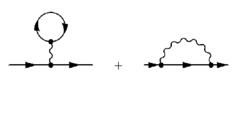
Figure 1: The second order diagrams contributing to the self-energy

$$\Sigma(k,i\omega_{n})_{\alpha,\beta}=$$

$$g^{2}\sum_{m\in even}\int[dq]e^{i\omega_{m}\eta}\mathcal{G}^{(0)}_{\alpha,\beta}(k+q,i\omega_{m})D^{(0)}(q,i\omega_{m}-i\omega_{n})\,,$$ (30)

where $\mathcal{G}^{(0)}(k,i\omega_{n})$ is the free electron propagator

$$\mathcal{G}^{(0)}(k,i\omega_{n})=\sum_{j}\frac{|u_{j}(k)\big{>}\big{<}u_{j}(k)|}{i\omega_{n}-(\epsilon_{j}(k)-\mu)}$$ (31)

and $D^{(0)}(k,i\omega_{n})$ is the free phonon propagator

$$D^{(0)}(k,i\omega_{n})=\frac{1}{i\omega_{n}-\omega_{0}}-\frac{1}{i\omega_{n}+\omega_{0}}\,.$$ (32)

Here $\omega_{n}$ is the Matsubara frequency, $\eta$ is the small positive number and $|u_{j}(k)\big{>}$ are the eigenvectors of the $H_{0}$ Hamiltonian. By summing over Matsubara frequencies we can find the following expression for the self energy.

$$\Sigma(k,i\omega_{n}) =\sum_{q}\sum_{\gamma=\pm}|u_{\gamma}(k+q)\big{>}\big{<}u_{\gamma}(k+q)|$$

$$\times\bigg{(}\frac{n_{f}[\epsilon_{j}(k+q)]+n_{b}[\omega_{0}]}{i\omega_{n}+\omega_{0}-(\epsilon_{j}(k+q)-\mu)}$$

$$+\frac{n_{b}[\omega_{0}]+1-n_{f}[\epsilon_{j}(k+q)]}{i\omega_{n}-\omega_{0}-(\epsilon_{j}(k+q)-\mu)}\bigg{)}\,.$$ (33)

If we analytically continue the imaginary-time self energy, we can find the life-time corresponding to the imaginary part of self-energy and the real part $\hat{\sigma}(k,\omega)$. In the limit $|\omega-\mu|\ll\omega_{0}$ and $T\rightarrow 0$, the imaginary part of the self energy vanishes but the real part remains finite even at $T=0$ Shindou and Balents (2008)

$$\hat{\sigma}(k,\omega)= g^{2}\sum_{\gamma=\pm}\bigg{[}\int_{\epsilon_{\gamma}(k^{\prime})\leq\mu}\mathcal{P}\frac{|u_{\gamma}(k^{\prime})\big{>}\big{<}u_{\gamma}(k^{\prime})|}{\omega+\omega_{0}-e_{\gamma}(k^{\prime})}$$

$$+\int_{\epsilon_{\gamma}(k^{\prime})\geq\mu}\mathcal{P}\frac{|u_{\gamma}(k^{\prime})\big{>}\big{<}u_{\gamma}(k^{\prime})|}{\omega-\omega_{0}-e_{\gamma}(k^{\prime})}\bigg{]}\frac{dk^{\prime}}{(2\pi)^{2}}\,,$$ (34)

where $e_{\gamma}(k)=\epsilon_{\gamma}(k)-\mu$. By using the results in section A we can write the projection operator as

$$|u^{\alpha}_{\gamma}(k)\big{>} \big{<}u^{\alpha}_{\gamma}(k)|=\frac{1}{2}\mathbf{1}+\frac{sign(\gamma)}{2}\bigg{[}cos(\theta_{k})\tau_{z}$$

$$-\alpha sin(\theta_{k})sin(\phi_{k})\tau_{x}+sin(\theta_{k})cos(\phi_{k})\tau_{y}\bigg{]}$$ (35)

Using the equation above, we can rewrite $\hat{\sigma}(\omega,k)$ as

$$\hat{\sigma}^{\alpha}(k,\omega)=S_{0}^{\alpha}(\omega)+S^{\alpha}_{1}(\omega)\tau_{z}-\alpha S^{\alpha}_{2}(\omega)\tau_{x}\,,$$ (36)

where

$$S^{\alpha}_{0}(\omega)= \frac{1}{2}\sum_{\gamma=\pm}\bigg{[}\int_{\epsilon^{\alpha}_{\gamma}(k)\leq\mu}\mathcal{P}\frac{1}{\omega+\omega_{0}-e^{\alpha}_{\gamma}(k^{\prime})}\frac{dk^{\prime}}{(2\pi)^{2}}$$

$$+\int_{\epsilon^{\alpha}_{\gamma}(k)\geq\mu}\mathcal{P}\frac{1}{\omega-\omega_{0}-e^{\alpha}_{\gamma}(k^{\prime})}\frac{dk^{\prime}}{(2\pi)^{2}}\bigg{]}\,,$$ (37)

$$S^{\alpha}_{1}(\omega)= \frac{g^{2}}{2}\sum_{\gamma=\pm}\bigg{[}\int_{\epsilon^{\alpha}_{\gamma}(k)\leq\mu}\mathcal{P}\frac{sign(\gamma)cos(\theta_{k^{\prime}})}{\omega+\omega_{0}-e^{\alpha}_{\gamma}(k^{\prime})}\frac{dk^{\prime}}{(2\pi)^{2}}$$

$$+\int_{\epsilon^{\alpha}_{\gamma}(k)\geq\mu}\mathcal{P}\frac{sign(\gamma)cos(\theta_{k^{\prime}})}{\omega-\omega_{0}-e^{\alpha}_{\gamma}(k^{\prime})}\frac{dk^{\prime}}{(2\pi)^{2}}\bigg{]}\,,$$ (38)

and

$$S^{\alpha}_{2}(\omega)=$$

$$\frac{g^{2}}{2}\sum_{\gamma=\pm}\bigg{[}\int_{\epsilon^{\alpha}_{\gamma}(k)\leq\mu}\mathcal{P}\frac{sign(\gamma)sin(\theta_{k^{\prime}})sin(\phi_{k^{\prime}})}{\omega+\omega_{0}-e^{\alpha}_{\gamma}(k^{\prime})}\frac{dk^{\prime}}{(2\pi)^{2}}$$

$$+\int_{\epsilon^{\alpha}_{\gamma}(k)\geq\mu}\mathcal{P}\frac{sign(\gamma)sin(\theta_{k^{\prime}})sin(\phi_{k^{\prime}})}{\omega-\omega_{0}-e^{\alpha}_{\gamma}(k^{\prime})}\frac{dk^{\prime}}{(2\pi)^{2}}\bigg{]}\,.$$ (39)

The coefficient of $\tau_{y}$ is zero because the Hamiltonian is invariant under $k_{x}\rightarrow-k_{x}$ and then the integral is odd under this symmetry. These coefficients can be calculated numerically as shown in Fig.[2].

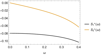
Figure 2: The functions $S_{1}(\omega)$ and $S_{2}(\omega)$ for $\Delta=0.5$, $v=1$, $s=1$, $\omega_{0}=0.5$ and $g=1$

III.3 AEF and Transport coefficients

For any two band systems, we can expand the effective Lagrangian in terms of Pauli matrices

$$\hat{L}(k,\omega)=\vec{N}(k,\omega).\vec{\tau}+C(k,\omega)\mathbf{1}\,,$$ (40)

where

$$\vec{N}(k,\omega)=\big{(}-\alpha\big{(}vk_{y}+S^{\alpha}_{2}(\omega)\big{)},\,vk_{x},\,\Delta+S_{1}(\omega)\big{)}\,,$$ (41)

and

$$C(k,\omega)=\alpha sk_{y}+S_{0}(\omega)\,,$$ (42)

We use the definition of the AMF and AEF in Shindou and Balents (2008) to compute these quantities.

$$\Omega^{\gamma}_{\alpha}(p)=-\frac{sign(\gamma)}{2}(\nabla_{kx}\hat{N}\times\nabla_{ky}\hat{N})\cdot\hat{N}$$ (43)

$$\mathcal{E}_{\gamma,k_{i}}=i\big{[}(\partial_{\omega}U)^{\dagger}\partial_{k_{i}}U-c.c\big{]}_{\gamma\gamma}\,,$$ (44)

where $U$ is the unitary operator which diagonalizes the effective Lagrangian.

$$U=\begin{pmatrix}cos(\frac{X}{2})&sin(\frac{X}{2})e^{-iY}\\ -sin(\frac{X}{2})e^{iY}&cos(\frac{X}{2})\end{pmatrix}$$ (45)

and

$$X=cos^{-1}\big{(}\frac{N_{z}}{|N|}\big{)}\,,$$ (46)

$$Y=tan^{-1}\big{(}\frac{N_{y}}{N_{x}}\big{)}\,.$$ (47)

Using Eq(45) and Eq(44), we can find the following equation for AEF

$$\mathcal{E}_{\gamma,k_{i}}=sign(\gamma)\bigg{(}(\partial_{\omega}Y)(\partial_{k_{i}}X)-(\partial_{k_{i}}Y)(\partial_{\omega}X)\bigg{)}\frac{sin(X)}{2}\,.$$ (48)

Using the definition of $\vec{N}(k,\omega)$ in Eq(41), we can find the AEF

$$\big{(}\mathcal{E}^{\alpha}_{\gamma,x},\mathcal{E}^{\alpha}_{\gamma,y}\big{)}= \frac{-sign(\gamma)v^{2}\alpha}{2(\Delta^{2}+v^{2}p^{2})^{3/2}}\frac{\partial S^{\alpha}_{1}(\omega)}{\partial\omega}(p_{y},-p_{x})$$

$$+ \frac{sign(\gamma)v\Delta\alpha}{2(\Delta^{2}+v^{2}p^{2})^{3/2}}\frac{\partial S^{\alpha}_{2}(\omega)}{\partial\omega}(1,0)\,.$$ (49)

Also, AMF can be calculated as

$$\Omega^{\gamma}_{\alpha}(p)=\frac{sign(\gamma)}{2}\frac{\alpha v^{2}\Delta}{(\Delta^{2}+v^{2}p^{2})^{3/2}}$$

$$+\frac{sign(\gamma)}{2}\frac{\alpha v^{2}}{(\Delta^{2}+v^{2}p^{2})^{3/2}}\bigg{(}\big{(}1-\frac{3\Delta^{2}}{(\Delta^{2}+v^{2}p^{2})}\big{)}S_{1}(\omega)\bigg{)}$$

$$+\frac{sign(\gamma)}{2}\frac{3k_{y}v^{3}\alpha\Delta}{(\Delta^{2}+v^{2}p^{2})^{5/2}}S^{\alpha}_{2}(\omega)\,,$$ (50)

where all the expressions should be evaluated at $\omega=\epsilon_{\gamma,p}^{(0)}$. AMF is matched with the results in Toshio et al. (2020) for a model without electron-phonon interaction. One can see the frequency dependence of the $\vec{N}$ is crucial to have a non-zero AEF and that comes from electron-phonon interaction in our model. To simplify the calculations, we can choose $\mu=0$. Also in weak strain limit, we can approximate the dispersion in Eq(22) as $\epsilon^{\alpha}_{\gamma}(k)\sim\frac{(p+p_{\alpha})^{2}}{2m}+\Delta+O(\frac{s}{v})^{2}$, where $m=\Delta/v^{2}$ and $p_{\alpha}=(0,\alpha s\Delta/v^{2})$. Finally, we can now estimate the magnitude of the AEF on the Fermi-surface $\omega=\mu$.

$$\big{(}\mathcal{E}^{\alpha}_{\gamma,x},\mathcal{E}^{\alpha}_{\gamma,y}\big{)}|_{\omega=0}=\frac{sign(\gamma)v^{2}\Delta}{(\Delta^{2}+v^{2}p^{2})^{3/2}}g^{2}sF(1,0)+O(\frac{s}{v})^{2}\,,$$ (51)

where

$$F=-\int\frac{k^{2}_{y}}{\lambda_{k}(\omega_{0}+\lambda_{k})^{3}}\frac{d^{2}k}{(2\pi)^{2}}\,.$$ (52)

In this model, all the contributions in AEF comes from $S^{\alpha}_{2}(\omega)$ because as one can see in Fig.[2], $\frac{\partial S^{\alpha}_{1}(\omega)}{\partial\omega}$ vanishes at $\omega=0$. By using these approximations, we can find the analytic expressions for the transport coefficients in section II at $T=0$.

$$\mathcal{G}_{xyy}=\frac{g^{2}sF}{4\pi}\big{[}-2\Delta+\frac{2\Delta^{2}+v^{2}P_{F}^{2}}{\sqrt{v^{2}P_{F}^{2}+\Delta^{2}}}\big{]}\,,$$ (53)

$$G_{xyy}=2g^{2}sF\frac{P_{F}^{2}}{(\Delta^{2}+v^{2}P_{F}^{2})^{3/2}}\,,$$ (54)

where $P_{F}=\sqrt{2m|\Delta|}$.

IV Effect of AEF on three-dimensional Poiseuille flow

In this part, we consider a 3D model with an external electric field in the $y$ direction. The system is bounded in the $x$ direction by the width $w$. To consider boundary effects, the viscosity term is introduced Kovtun (2012):

$$\Pi_{ij}=\rho u_{i}u_{j}+P\delta_{ij}-\Sigma_{ij}\,,$$ (55)

where

$$\Sigma_{ij}=\rho\nu(\partial_{i}u_{j}+\partial_{j}u_{i}-\frac{2}{3}\delta_{ij}\partial_{k}u_{k})+\xi\delta_{ij}\partial_{k}u_{k}\,.$$ (56)

Here $\nu$ is the shear viscosity and $\xi$ is the bulk viscosity, which we are going to ignore.

Now we use an ansatz as a solution, which is $u_{x}=u_{z}=0$ and $u_{y}=u_{y}(x)$. So the hydrodynamic equation Eq(12) becomes:

$$-\rho\nu\partial^{2}_{x}u_{y}+neE=-\rho\frac{u_{y}}{\tau_{mr}}\,.$$ (57)

The solution for the above equation with the boundary condition $u(\frac{w}{2})=u(-\frac{w}{2})=0$ is given by:

$$u_{y}=\frac{e\tau_{mr}E}{m}(1-\frac{cosh(x/l)}{cosh(w/2l)})\,,$$ (58)

which is a standing wave solution in the $x$ direction, where

$$l=\sqrt{\nu\tau_{mr}}\,,$$ (59)

and the vorticity is:

$$\omega_{z}(x)=\frac{\partial u_{y}}{\partial x}=\frac{e\tau_{mr}E}{ml}\frac{sinh(x/l)}{cosh(w/2l)}\,.$$ (60)

Now when we have the vorticity, we can compute the on-shell current by using Eq(16):

$$J_{i}=nu_{i}\delta_{i,y}+e\epsilon_{ixl}C_{yl}\partial_{x}u_{y}+emG_{iyy}E_{y}u_{y}-e\mathcal{G}_{ixy}\partial_{x}u_{y}\,.$$ (61)

As a result we can see that there are contributions in all directions, which come from AEF.

$$J_{x}=-e^{2}mG_{xyy}Eu_{y}\,,$$ (62)

$$J_{y}=-enu_{y}+e^{2}C_{yz}\omega_{z}+e^{2}\mathcal{G}_{zxy}\omega_{z}\,,$$ (63)

$$J_{z}=-e^{2}C_{yy}\omega_{z}-e^{2}mG_{zyy}Eu_{y}+e^{2}\mathcal{G}_{zxy}\omega_{z}\,.$$ (64)

The $G_{xyy}$ and $G_{zyy}$ terms are non-linear contributions to the currents, $\mathcal{G}_{zxy}$ and $C_{il}$ terms are linear contributions.

V Conclusion and outlook

We demonstrate that the AEF introduces a number of novel hydrodynamic and non-linear transport coefficients in the time-reversal invariant systems with broken inversion symmetry. In the example of a two-dimensional electron system, we show how these novel transport coefficients arise from the electron-phonon interaction. For instance, it is shown that there is a non-linear transport current along the $x$-direction when the electric field is applied along the $y$-direction, that is $J_{x}=G_{xyy}E_{y}E_{y}$ with a finite $G_{xyy}$. In similar spirit, the Poiseuille flow in the three-dimensional system in a constriction would allow non-uniform (non-linear) transport currents in all three directions. This is in contrast to the usual case, where the non-uniform current exists only along the direction of the applied electric field or even to the case when the AMF effect is included, where there exist the Poiseuille flow in two directions via the presence of the finite vorticity field Toshio et al. (2020).

Our work sheds light on novel non-linear transport and hydrodynamic phenomena in ultra-pure strongly-interacting electron systems. Such systems are great platforms for the discovery of the intricate quantum effects associated with the rather elusive AEF. It will also be interesting to explore further consequences of the AEF in other non-linear electromagnetic responses, both theoretically and experimentally.

Appendix A Hydrodynamics

Here we drive the hydrodynamic equation and constitutive relations for the conserved quantities. To find the hydrodynamic relations, we start with modified EoMs:

$$\dot{\vec{r}}_{n}=\vec{v}_{n}+(\vec{\Omega}_{n}-\vec{\mathcal{E}}_{n}\times\vec{v}_{n})\times\dot{\vec{k}}_{n}\,,$$ (65)

$$\dot{\vec{k}}_{n}=-e\vec{E}\,,$$ (66)

where $\Omega$ is the Berry curvature, $\mathcal{E}$ is an artificial electric field, $E$ is electric field. we can see this as a two equation with two unknown variables $\dot{k}_{n}$ and $\dot{r}_{n}$ which need to be solved.

Using $\dot{k}$ in Eq(66) and Eq(65) we can find:

$$\dot{\vec{r}}=\vec{v}+eE\times(\vec{\Omega}-\vec{\mathcal{E}}\times\vec{v})\,,$$ (67)

When we find $\dot{k}$ and $\dot{r}$ we can write the Boltzmann equation:

$$\frac{\partial f}{\partial t}+\big{(}\vec{v}+e\vec{E}\times(\vec{\Omega}-\vec{\mathcal{E}}\times\vec{v})\big{)}\cdot\nabla_{r}f-e\vec{E}\cdot\nabla_{k}f=\mathcal{C}[f]\,.$$ (68)

We can find hydrodynamic equations by multiplying the above equation by momentum and integrate over the momentum space that we can find the following equation

$$\frac{\partial}{\partial t}\int[dk]\vec{k}f +\nabla_{r}\cdot\int[dk]\big{(}\vec{v}+e\vec{E}\times(\vec{\Omega}-\vec{\mathcal{E}}\times\vec{v})\big{)}\vec{k}f-e\vec{E}\int[dk]\vec{k}\cdot\nabla_{k}f=\int[dk]\vec{k}\,\mathcal{C}[f]\,,$$ (69)

which is the extended hydrodynamic equation for quasi-conserved quantity, momentum.

$$\frac{\partial\vec{P}}{\partial t}+\vec{\nabla}.\Pi+n\vec{E}=-\frac{\vec{P}}{\tau_{mr}}\,,$$ (70)

where we can define momentum density and modified stress tensor as follows

$$\vec{P}=\int[dp]\vec{p}f\,,$$ (71)

$$\Pi_{ij}=\int[dp]p_{i}\big{(}\vec{v}+e\vec{E}\times\vec{\Omega}-e\vec{E}\times(\vec{\mathcal{E}}\times\vec{v})_{j}\big{)}_{j}f\,.$$ (72)

In the right hand side of the Eq(68), we consider the collision term $C[f]=C_{mc}[f]+C_{mr}[f]$ where the first term is related to the collisions that conserve momentum, and the second term is related to the collisions that relax the momentum. So after integration the first term vanishes and we can parametrize the second term with $\frac{f(t,r,p)}{\tau_{mr}}$ in relaxation time approximation.

To find the constitutive relations for momentum and stress tensor we expand the distribution function in terms of hydrodynamic variables. In the following we assume that the underlying effective theory is invariant under Galilean transformation $f_{0}(\vec{p})=f_{u}(\vec{p}+m\vec{u})$.

To find a relation for the momentum we use Eq(71)

$$\vec{P}= \int[dp]\vec{p}f_{u}(p)=\int[dp](\vec{p}+m\vec{u})f_{0}(p)=mn\vec{u}\,,$$ (73)

where $n=\int[dp]f_{0}(p)$. By the same approach we find the constitutive relation for stress tensor using Eq(72), which we rewrite it as

$$\Pi_{ij} =\sum_{n}\int[dp]p_{i}v_{j,n}f_{u}(p,n)+\int[dp]p_{i}\big{(}eE\times\Omega_{n}(p)-eE\times(\mathcal{E}_{n}(p)\times v_{n})\big{)}_{j}f_{u}(p,n)\,,$$ (74)

where $n$ is the band index and the first term in the rhs of the above equation is the standard terms for stress tensor in hydrodynamic regime $\int[dp]p_{i}v_{j}=\rho u_{i}u_{j}+P\delta_{ij}$. The second term is the anomalous part which we are going to investigate in the following. We denote the first anomalous part as $\Pi^{\Omega}_{ij}$ which means the AMF contributions to the stress tensor.

$$\Pi^{\Omega}_{ij} =\epsilon_{klj}E_{k}\sum_{n}\int[dp]p_{i}\Omega^{l}_{n}f_{u}$$

$$=\epsilon_{klj}E_{k}\int[dp](p_{i}+mu_{i})\Omega^{l}_{n}(p+m\vec{u})f_{0}(p)$$

$$=\epsilon_{klj}E_{k}\int[dp](p_{i}+mu_{i})\big{(}\Omega^{l}_{n}+\frac{\partial\Omega^{l}_{n}}{\partial p_{r}}mu_{r}\big{)}f_{0}(p)\,,$$ (75)

up to the second order in $u$ and $E$ we have

$$\Pi^{\Omega}_{ij}= \sum_{n}\epsilon_{klj}E_{k}\bigg{(}\int[dp]p_{i}\Omega^{l}_{n}f_{0}+\int[dp]p_{i}\frac{\partial\Omega^{l}_{n}}{\partial p_{r}}f_{0}\,mu_{r}+mu_{i}\int[dp]\Omega^{l}_{n}f_{0}\bigg{)}\,.$$ (76)

The second term is zero due to time-reversal symmetry($\Omega_{l}\rightarrow-\Omega_{l},p\rightarrow-p$) and the third term is zero because the sum of berry charge over each valley is zero. Finally

$$\Pi^{\Omega}_{ij}=e\epsilon_{klj}E_{k}C_{il}\,,$$ (77)

where

$$C_{il}=\sum_{n}\int[dp]p_{i}\Omega^{l}_{n}f_{0}(p)\,.$$ (78)

In the following, without loss of generality, we can drop the band index and finally we sum over all bands. For the second part of the anomalous term $\Pi^{\mathcal{E}}_{ij}$ we have

$$-e\int[dp]p_{i}E\times(\mathcal{E}\times v)_{j}f_{u}=-e\epsilon_{klj}E_{k}\int[dp]p_{i}(\mathcal{E}\times v)_{l}f_{u}=-e\epsilon_{klj}\epsilon_{mnl}E_{k}\int[dp]p_{i}\mathcal{E}_{m}v_{n}f_{u}$$

$$=-e(\delta_{jm}\delta_{kn}-\delta_{jn}\delta_{km})E_{k}\int[dp](p_{i}+mu_{i})\mathcal{E}_{m}(p+m\vec{u})v_{n}(p+m\vec{u})f_{0}$$

$$=-e(\delta_{jm}\delta_{kn}-\delta_{jn}\delta_{km})E_{k}\int[dp](p_{i}+mu_{i})(\mathcal{E}_{m}+\frac{\partial\mathcal{E}_{m}}{\partial p_{b}}mu_{b})(v_{n}+\frac{\partial v_{n}}{\partial p_{a}}mu_{a})f_{0}$$

$$=-eE_{k}\int[dp](p_{i}+mu_{i})\bigg{[}(\mathcal{E}_{j}+\frac{\partial\mathcal{E}_{j}}{\partial p_{b}}mu_{b})(v_{k}+\frac{\partial v_{k}}{\partial p_{a}}mu_{a})-(j\leftrightarrow k)\bigg{]}f_{0}\Rightarrow$$

$$\Pi^{\mathcal{E}}_{ij}=-eE_{k}\bigg{(}\int[dp]p_{i}\mathcal{E}_{j}v_{k}f_{0}+mu_{i}\int[dp]\mathcal{E}_{j}v_{k}f_{0}+mu_{l}\int[dp]p_{i}v_{k}\frac{\partial\mathcal{E}_{j}}{\partial p_{l}}f_{0}+mu_{l}\int[dp]p_{i}\mathcal{E}_{j}\frac{\partial v_{k}}{\partial p_{l}}f_{0}\bigg{)}\,.$$ (79)

The first term is odd under Inversion symmetry and even under Time-reversal. The second,third and forth terms are odd under Time-reversal and even under Inversion. So if we consider Time-reversal invariant Noncentrosymmetric system then only the first term is non-zero. Finally we can write the new contribution to the stress tensor as the following

$$\Pi^{\mathcal{E}}_{ij}=eE_{k}\mathcal{G}_{kji}\,,$$ (80)

where

$$\mathcal{G}_{ijk}=\sum_{n}\int[dp](\mathcal{E}^{n}_{i}v^{n}_{j}-\mathcal{E}^{n}_{j}v^{n}_{i})p_{k}f^{n}_{0}\,.$$ (81)

By finding all the contributions we can write the stress tensor as

$$\Pi_{ij}=\rho u_{i}u_{j}+P\delta_{ij}+e\epsilon_{klj}C_{il}E_{k}+e\mathcal{G}_{kji}E_{k}\,.$$ (82)

Now we find the transport current which is made of particle flux $\vec{J}^{N}$ and orbital magnetization.

$$\vec{J}=\vec{J}^{N}+\nabla\times\vec{M}\,,$$ (83)

where

$$\vec{J}^{N}=\sum_{n}\int[dp]\dot{\vec{r}}f_{u}=\int[dp](\vec{v}_{n}+e\vec{E}\times(\vec{\Omega}_{n}-\vec{\mathcal{E}}_{n}\times\vec{v}_{n}))f^{n}_{u}\,$$ (84)

and

$$\vec{M}=\sum_{n}\frac{e}{\beta}\int[dp](\vec{\Omega}_{n}-\vec{\mathcal{E}}_{n}\times\vec{v}_{n})\log(1+e^{-\beta(\epsilon_{n}-\vec{u}\cdot\vec{p}-\mu)})\,.$$ (85)

Using the Galilean symmetry and expanding up to second order in $u$ and $E$ we find (we should note we drop the band index)

$$J^{N}_{i}= \int[dp]\bigg{[}v+\frac{\partial v}{\partial p_{j}}mu_{j}+eE\times\Omega+eE\times\frac{\partial\Omega}{\partial p_{j}}mu_{j}\bigg{]}f_{0}$$

$$-eE\times\int[dp]\bigg{[}\mathcal{E}\times v+\mathcal{E}\times\frac{\partial v}{\partial p_{j}}mu_{j}+mu_{j}\frac{\partial\mathcal{E}}{\partial p_{j}}\times v\bigg{]}f_{0}$$ (86)

We separate the terms in particle flux like what we did for stress tensor,

$$\vec{J}^{N}=\rho\vec{u}+\vec{J}_{\Omega}+\vec{J}_{\mathcal{E}}\,,$$ (87)

where

$$J^{N}_{\Omega,i}=eE_{k}mu_{j}\epsilon_{kli}\int[dp]\frac{\partial\Omega_{l}}{\partial p_{j}}f_{0}\,.$$ (88)

Using integrating by part:

$$J_{\Omega,i}=-eE_{k}mu_{j}\epsilon_{kli}\int[dp]\Omega_{l}\frac{\partial f_{0}}{\partial p_{j}}=(em)E_{k}u_{j}\epsilon_{kli}D_{jl}\,,$$ (89)

where

$$D_{il}=-\sum_{n}\int[dp]\Omega^{n}_{l}\frac{\partial f^{n}_{0}}{\partial p_{i}}\,.$$ (90)

Now for $J^{N}_{\mathcal{E}}$ in Eq(86) we have

$$J^{N}_{\mathcal{E}}=-eE\times\int[dp]\bigg{[}\mathcal{E}\times v+\mathcal{E}\times\frac{\partial v}{\partial p_{j}}mu_{j}+mu_{j}\frac{\partial\mathcal{E}}{\partial p_{j}}\times v\bigg{]}f_{0}$$ (91)

If we consider TRS system ($\mathcal{E}\rightarrow\mathcal{E}$, $\vec{p}\rightarrow-\vec{p}$ and $\vec{v}\rightarrow-\vec{v}$)then the first term in $J_{\mathcal{E}}$ vanish. Using integration by part we find

$$J_{\mathcal{E},i}=eE_{m}\epsilon_{iml}\epsilon_{nkl}\int[dp]\mathcal{E}_{n}v_{k}\frac{\partial f_{0}}{\partial p_{j}}mu_{j}$$

$$\Rightarrow J_{\mathcal{E},i}= eE_{k}mu_{j}\int[dp](\mathcal{E}_{i}v_{k}-\mathcal{E}_{k}v_{i})\frac{\partial f_{0}}{\partial p_{j}}=(em)G_{ikj}E_{k}u_{j}\,,$$ (92)

where

$$G_{ijk}=\sum_{n}\int[dp](\mathcal{E}^{n}_{i}v^{n}_{j}-\mathcal{E}^{n}_{j}v^{n}_{i})\frac{\partial f^{n}_{0}}{\partial p_{k}}\,.$$ (93)

Now for the orbital magnetization part we have the same separation and expansion, $\vec{M}=\vec{M}^{\Omega}+\vec{M}^{\mathcal{E}}$

$$\vec{M}^{\Omega}=\frac{e}{\beta}\int[dp]\vec{\Omega}_{p}log\big{(}1+e^{-\beta(\epsilon-u.p-\mu)}\big{)}$$

$$\Rightarrow M^{\Omega}_{i}=eu_{l}\int[dp]\Omega_{i}p_{l}f_{0}+O(u^{2})=eu_{l}C_{li}+O(u^{2})$$ (94)

$$(\nabla\times\vec{M}^{\Omega})_{k} =\epsilon_{jik}\partial_{j}M_{i}=e\epsilon_{jik}\partial_{j}(u_{l}C_{li})=e\epsilon_{jik}C_{li}\partial_{j}u_{l}+e\epsilon_{jik}u_{l}\partial_{j}C_{li}\,.$$ (95)

We can expand the $\partial_{j}C_{li}$ term:

$$\partial_{j}C_{li}= -\beta\frac{\partial C_{li}}{\partial\beta}(\frac{\partial_{j}T}{T})+\frac{\partial C_{li}}{\partial\mu}\partial_{j}\mu$$

$$=mF_{li}\frac{\partial_{j}T}{T}+mD_{li}\partial_{j}\mu\,,$$ (96)

where

$$\frac{\partial C_{li}}{\partial\mu}= -\int[dp]p_{l}\Omega_{i}\frac{\partial f_{0}}{\partial\epsilon}=m\int[dp]\Omega_{i}\frac{\partial\epsilon}{\partial p_{l}}\frac{\partial f}{\partial\epsilon}$$

$$=m\int[dp]\Omega_{i}\frac{\partial f}{\partial p_{l}}=mD_{li}$$ (97)

and

$$F_{il}=\sum_{n}\frac{-\beta}{m}\int[dp]\Omega^{n}_{l}p_{i}\frac{\partial f^{n}_{0}}{\partial\beta}\,.$$ (98)

For $\vec{M}^{\mathcal{E}}$ we use similar approach

$$\vec{M}_{\mathcal{E}}=-\frac{e}{\beta}\int[dp](\vec{\mathcal{E}}\times\vec{v})log\big{(}1+e^{-\beta(\epsilon-u.p-\mu)}\big{)}$$

$$\Rightarrow\vec{M}^{\mathcal{E}}=-e\int[dp](\vec{\mathcal{E}}\times\vec{v})(\vec{p}\cdot\vec{u})f_{0}+O(u^{2})\,.$$ (99)

Now we can calculate $(\nabla\times\vec{M}_{\mathcal{E}})_{k}$

$$(\nabla\times\vec{M}_{\mathcal{E}})_{k}=-e\epsilon_{ijk}\partial_{i}\int[dp]\epsilon_{nlj}\mathcal{E}_{n}v_{l}(p.u)f_{0}$$

$$=(\delta_{in}\delta_{kl}-\delta_{il}\delta_{kn})\int[dp]\mathcal{E}_{n}v_{l}(p.u)\partial_{i}f_{0}$$

$$=\int[dp](\mathcal{E}_{i}v_{k}-\mathcal{E}_{k}v_{i})(p.u)\big{(}-\beta\frac{\partial f_{0}}{\partial\beta}(\frac{\partial_{i}T}{T})+\frac{\partial f_{0}}{\partial\mu}\partial_{i}\mu\big{)}$$

$$+\int[dp](\mathcal{E}_{i}v_{k}-\mathcal{E}_{k}v_{i})(p_{j}\partial_{i}u_{j})f_{0}\,.$$ (100)

By considering the parabolic dispersion relation the above equation can be written as the following form

$$(\nabla\times\vec{M}^{\mathcal{E}})_{k}=I_{kij}(\frac{\partial_{i}T}{T})u_{j}+G_{kij}\partial_{i}\mu u_{j}+\mathcal{G}_{ikj}\partial_{i}u_{j}\,,$$ (101)

where

$$I_{ijk}=\sum_{n}\frac{\beta}{m}\int[dp](\mathcal{E}^{n}_{i}v^{n}_{j}-\mathcal{E}^{n}_{j}v^{n}_{i})p_{k}\frac{\partial f^{n}_{0}}{\partial\beta}$$ (102)

Finally we can write the final expression for the transport current Eq(83)

$$J_{i} =nu_{i}+em\epsilon_{ikl}(E_{k}+\partial_{k}\mu)D_{jl}u_{j}+em\epsilon_{ikl}(\frac{\partial_{k}T}{T})F_{jl}u_{j}$$

$$+\epsilon_{ikl}C_{jl}\partial_{k}u_{j}+emG_{ikj}(E_{k}+\partial_{k}\mu)u_{j}$$

$$+emI_{ikj}(\frac{\partial_{k}T}{T})u_{j}-e\mathcal{G}_{ikj}\partial_{k}u_{j}$$ (103)

Using constitutive relations and Eq(70) we can find a hydrodynamic equation

$$\rho\frac{\partial u_{i}}{\partial t}+\rho u_{j}\partial_{j}u_{i}+\partial_{i}P+em\epsilon_{jkl}E_{k}\big{[}F_{il}\frac{\partial_{j}T}{T}+D_{il}\partial_{j}\mu\big{]}$$

$$+e\epsilon_{jkl}C_{il}\partial_{j}E_{k}+emE_{k}\big{[}I_{jki}\frac{\partial_{j}T}{T}+G_{jki}\partial_{j}\mu\big{]}$$

$$+e\mathcal{G}_{kji}\partial_{j}E_{k}+enE_{i}=-\rho\frac{u_{i}}{\tau_{mr}}\,,$$ (104)

where we used following relation for coefficients

$$\partial_{j}\mathcal{G}_{kji}=\frac{\mathcal{G}_{kji}}{\partial T}\partial_{j}T+\frac{\mathcal{G}_{kji}}{\partial\mu}\partial_{j}\mu=mI_{jki}\frac{\partial_{j}T}{T}+mG_{jki}\partial_{j}\mu\,.$$ (105)

Appendix B The model

Here, we outline the calculation of transport coefficients in a specific Hamiltonian model

$$H=H^{\alpha}_{0}+H_{ph}+H_{ep}\,,$$ (106)

where

$$H^{\alpha}_{0}(\vec{k})=\alpha sk_{y}\mathbf{1}+vk_{x}\tau_{y}-\alpha vk_{y}\tau_{x}+\Delta\tau_{z}\,,$$ (107)

$$H_{ph}=\sum_{q}\omega_{0}b^{\dagger}_{q}b_{q}$$ (108)

and

$$H_{ep}=g\sum_{k,q,\alpha}\psi^{\dagger}_{\alpha}(k+q)\psi_{\alpha}(k)(b_{q}+b^{\dagger}_{-q})\,.$$ (109)

Using perturbation theory we have the following expression for the first order correction to the green’s function

$$\mathcal{G}^{(1)}(k,i\omega_{n})=\mathcal{G}^{(0)}\Sigma(k,i\omega_{n})\,\mathcal{G}^{(0)}\,,$$ (110)

where we can define the self energy as

$$\Sigma(k,i\omega_{n})_{\alpha,\beta}=g^{2}\sum_{m\in odd}\int[dq]e^{i\omega_{m}\eta}\mathcal{G}^{(0)}_{\alpha,\beta}(k+q,i\omega_{m})D^{(0)}(q,i\omega_{m}-i\omega_{n})$$

$g^{(0)}$ and $D^{(0)}$ are defined by the free electron and phonon’s Hamiltonian:

$$\mathcal{G}^{(0)}(k,i\omega_{n})=\sum_{\gamma}\frac{|u^{\alpha}_{\gamma}(k)\big{>}\big{<}u^{\alpha}_{\gamma}(k)|}{i\omega_{n}-(\epsilon^{\alpha}_{\gamma}(k)-\mu)}\,,$$ (111)

$$D^{(0)}(k,i\omega_{n})=\frac{1}{i\omega_{n}-\omega_{0}}-\frac{1}{i\omega_{n}+\omega_{0}}\,,$$ (112)

where $\epsilon^{\alpha}_{\gamma}(\vec{k})=\alpha sk_{y}+\gamma\lambda(k)$ is the eigenvalue of the $H_{0}$ , $k=\sqrt{k_{x}^{2}+k_{y}^{2}}$ and $\lambda(k)=\sqrt{(vk)^{2}+\Delta^{2}}$. Also for the eigenvectors we have

$$|u^{\alpha}_{+}(\vec{k})\big{>}=\begin{pmatrix}cos(\frac{\theta_{k}}{2})\\ sin(\frac{\theta_{k}}{2})e^{i\phi^{\alpha}_{k}}\end{pmatrix}\,,$$ (113)

$$|u^{\alpha}_{-}(\vec{k})\big{>}=\begin{pmatrix}-sin(\frac{\theta_{k}}{2})e^{-i\phi^{\alpha}_{k}}\\ cos(\frac{\theta_{k}}{2})\end{pmatrix}\,,$$ (114)

where

$$\phi^{\alpha}_{k}=\alpha\phi_{k}+\frac{\pi}{2}\,,$$ (115)

$$(cos(\theta_{k}),sin(\theta_{k}))=\frac{1}{\lambda_{k}}(\Delta,vk)$$ (116)

and

$$(cos(\phi_{k}),sin(\phi_{k}))=(\frac{k_{x}}{k},\frac{k_{y}}{k})\,.$$ (117)

Using Eq(B), Eq(111) and Eq(112) we can find

$$\Sigma^{\alpha}(k,i\omega_{n})=\sum_{m\in odd}\int[dq]e^{i\omega_{m}\eta}\sum_{\gamma}\frac{|u^{\alpha}_{\gamma}(k+q)\big{>}\big{<}u^{\alpha}_{\gamma}(k+q)|}{i\omega_{m}-(\epsilon^{\alpha}_{\gamma}(k+q)-\mu)}\big{(}\frac{1}{i\omega_{m}-i\omega_{n}-\omega_{0}}-\frac{1}{i\omega_{m}-i\omega_{n}+\omega_{0}}\big{)}$$ (118)

where $\eta$ is a small positive number. By calculating the following expression

$$\sum_{m\in odd}e^{i\omega_{m}\eta}\frac{1}{i\omega_{m}-e^{\alpha}_{\gamma}(k+q)}\frac{1}{i\omega_{m}-i\omega_{n}-\omega_{0}}$$

$$=\frac{1}{i\omega_{n}+\omega_{0}-e^{\alpha}_{\gamma}(k+q)}\sum_{m\in even}e^{i\omega_{m}\eta}\big{[}\frac{1}{i\omega_{m}-i\omega_{n}-\omega_{0}}-\frac{1}{i\omega_{m}-e^{\alpha}_{\gamma}(k+q)}\big{]}$$

$$=\frac{1}{i\omega_{n}+\omega_{0}-e^{\alpha}_{\gamma}(k+q)}\big{(}n_{f}[e^{\alpha}_{\gamma}(k+q)]+n_{b}[\omega_{0}]\big{)}\,,$$ (119)

and summing over Matsubara frequencies in Eq(118) we can find

$$\Sigma(k,i\omega_{n}) =\sum_{q}\sum_{\gamma=\pm}|u_{\gamma}(k+q)\big{>}\big{<}u_{\gamma}(k+q)|\bigg{(}\frac{n_{f}[e_{j}(k+q)]+n_{b}[\omega_{0}]}{i\omega_{n}+\omega_{0}-e_{j}(k+q)}+\frac{n_{b}[\omega_{0}]+1-n_{f}[e_{j}(k+q)]}{i\omega_{n}-\omega_{0}-e_{j}(k+q)}\bigg{)}\,.$$ (120)

Using analytic continuation, in the limit $|\omega-\mu|\ll\omega_{0}$ and $T\rightarrow 0$, we can find the real part of the self energy as the following

$$\sigma(k,\omega)= g^{2}\sum_{\gamma=\pm}\bigg{[}\int_{\epsilon_{\gamma}(k^{\prime})\leq\mu}\mathcal{P}\frac{|u_{\gamma}(k^{\prime})\big{>}\big{<}u_{\gamma}(k^{\prime})|}{\omega+\omega_{0}-e_{\gamma}(k^{\prime})}+\int_{\epsilon_{\gamma}(k^{\prime})\geq\mu}\mathcal{P}\frac{|u_{\gamma}(k^{\prime})\big{>}\big{<}u_{\gamma}(k^{\prime})|}{\omega-\omega_{0}-e_{\gamma}(k^{\prime})}\bigg{]}\frac{dk^{\prime}}{(2\pi)^{2}}\,.$$ (121)

The projection operator for the mentioned model is

$$|u^{\alpha}_{\gamma}(k)\big{>} \big{<}u^{\alpha}_{\gamma}(k)|=\frac{1}{2}\mathbf{1}+\frac{sign(\gamma)}{2}\bigg{[}cos(\theta_{k})\tau_{z}-\alpha sin(\theta_{k})sin(\phi_{k})\tau_{x}+sin(\theta_{k})cos(\phi_{k})\tau_{y}\bigg{]}\,.$$

Using projection operator in Eq(121) we can find

$$\sigma^{\alpha}(k,\omega) =\frac{1}{2}\sum_{\gamma=\pm}\bigg{[}\int_{\epsilon^{\alpha}_{\gamma}(k)\leq\mu}\mathcal{P}\frac{1}{\omega+\omega_{0}-e^{\alpha}_{\gamma}(k^{\prime})}\frac{dk^{\prime}}{(2\pi)^{2}}+\int_{\epsilon^{\alpha}_{\gamma}(k)\geq\mu}\mathcal{P}\frac{1}{\omega-\omega_{0}-e^{\alpha}_{\gamma}(k^{\prime})}\frac{dk^{\prime}}{(2\pi)^{2}}\bigg{]}\mathbf{1}$$

$$+\tau_{z}\frac{g^{2}}{2}\sum_{\gamma=\pm}\bigg{[}\int_{\epsilon^{\alpha}_{\gamma}(k)\leq\mu}\mathcal{P}\frac{sign(\gamma)cos(\theta_{k^{\prime}})}{\omega+\omega_{0}-e^{\alpha}_{\gamma}(k^{\prime})}\frac{dk^{\prime}}{(2\pi)^{2}}+\int_{\epsilon^{\alpha}_{\gamma}(k)\geq\mu}\mathcal{P}\frac{sign(\gamma)cos(\theta_{k^{\prime}})}{\omega-\omega_{0}-e^{\alpha}_{\gamma}(k^{\prime})}\frac{dk^{\prime}}{(2\pi)^{2}}\bigg{]}$$

$$-\alpha\tau_{x}\frac{g^{2}}{2}\sum_{\gamma=\pm}\bigg{[}\int_{\epsilon^{\alpha}_{\gamma}(k)\leq\mu}\mathcal{P}\frac{sign(\gamma)sin(\theta_{k^{\prime}})sin(\phi_{k^{\prime}})}{\omega+\omega_{0}-e^{\alpha}_{\gamma}(k^{\prime})}\frac{dk^{\prime}}{(2\pi)^{2}}+\int_{\epsilon^{\alpha}_{\gamma}(k)\geq\mu}\mathcal{P}\frac{sign(\gamma)sin(\theta_{k^{\prime}})sin(\phi_{k^{\prime}})}{\omega-\omega_{0}-e^{\alpha}_{\gamma}(k^{\prime})}\frac{dk^{\prime}}{(2\pi)^{2}}\bigg{]}\,.$$ (122)

The coefficient of $\tau_{y}$ term vanishes because it is an odd function on $k^{\prime}_{x}$. Now we can write the above equation in a simpler form

$$\hat{\sigma}^{\alpha}(k,\omega)=S_{0}^{\alpha}(\omega)+S^{\alpha}_{1}(\omega)\tau_{z}-\alpha S^{\alpha}_{2}(\omega)\tau_{x}$$ (123)

where

$$S^{\alpha}_{0}(\omega)=\frac{1}{2}\sum_{\gamma=\pm}\bigg{[}\int_{\epsilon^{\alpha}_{\gamma}(k)\leq\mu}\mathcal{P}\frac{1}{\omega+\omega_{0}-e^{\alpha}_{\gamma}(k^{\prime})}\frac{dk^{\prime}}{(2\pi)^{2}}+\int_{\epsilon^{\alpha}_{\gamma}(k)\geq\mu}\mathcal{P}\frac{1}{\omega-\omega_{0}-e^{\alpha}_{\gamma}(k^{\prime})}\frac{dk^{\prime}}{(2\pi)^{2}}\bigg{]}\,,$$ (124)

$$S^{\alpha}_{1}(\omega)=\frac{g^{2}}{2}\sum_{\gamma=\pm}\bigg{[}\int_{\epsilon^{\alpha}_{\gamma}(k)\leq\mu}\mathcal{P}\frac{sign(\gamma)cos(\theta_{k^{\prime}})}{\omega+\omega_{0}-e^{\alpha}_{\gamma}(k^{\prime})}\frac{dk^{\prime}}{(2\pi)^{2}}+\int_{\epsilon^{\alpha}_{\gamma}(k)\geq\mu}\mathcal{P}\frac{sign(\gamma)cos(\theta_{k^{\prime}})}{\omega-\omega_{0}-e^{\alpha}_{\gamma}(k^{\prime})}\frac{dk^{\prime}}{(2\pi)^{2}}\bigg{]}\,,$$ (125)

and

$$S^{\alpha}_{2}(\omega)= \frac{g^{2}}{2}\sum_{\gamma=\pm}\bigg{[}\int_{\epsilon^{\alpha}_{\gamma}(k)\leq\mu}\mathcal{P}\frac{sign(\gamma)sin(\theta_{k^{\prime}})sin(\phi_{k^{\prime}})}{\omega+\omega_{0}-e^{\alpha}_{\gamma}(k^{\prime})}\frac{dk^{\prime}}{(2\pi)^{2}}+\int_{\epsilon^{\alpha}_{\gamma}(k)\geq\mu}\mathcal{P}\frac{sign(\gamma)sin(\theta_{k^{\prime}})sin(\phi_{k^{\prime}})}{\omega-\omega_{0}-e^{\alpha}_{\gamma}(k^{\prime})}\frac{dk^{\prime}}{(2\pi)^{2}}\bigg{]}\,.$$ (126)

Now one can write the effective Lagrangian $\hat{L}(k,\omega)=H_{0}(k)+\hat{\sigma}(k,\omega)$ as an expansion of Pauli matrices $\hat{L}(k,\omega)=N_{\mu}\tau_{\mu}+C(k,\omega)\mathbf{1}$

$$\hat{L}(k,\omega)=-\alpha\big{(}vk_{y}+S^{\alpha}_{2}(\omega)\big{)}\tau_{x}+vk_{x}\tau_{y}+(\Delta+S_{1}(\omega))\tau_{z}+(\alpha sk_{y}+S_{0}(\omega))\mathbf{1}\,,$$ (127)

where

$$N_{\mu}=\big{(}-\alpha\big{(}vk_{y}+S^{\alpha}_{2}(\omega)\big{)},\,vk_{x},\,\Delta+S_{1}(\omega)\big{)}\,.$$ (128)

To find the AMF we use following definition

$$\Omega^{\gamma}_{\alpha}(p)=-\frac{sign(\gamma)}{2}(\nabla_{kx}\hat{N}\times\nabla_{ky}\hat{N}).\hat{N}$$

$$\Rightarrow\Omega^{\gamma}_{\alpha}(p)=\frac{sign(\gamma)}{2}\frac{\alpha v^{2}}{(\Delta^{2}+v^{2}p^{2})^{3/2}}\bigg{(}\Delta+\big{(}1-\frac{3\Delta^{2}}{(\Delta^{2}+v^{2}p^{2})}\big{)}S_{1}(\omega)|_{\omega=\epsilon_{\gamma,p}^{(0)}}\bigg{)}\frac{sign(\gamma)}{2}\frac{3k_{y}v^{3}\alpha\Delta}{(\Delta^{2}+v^{2}p^{2})^{5/2}}S^{\alpha}_{2}(\omega)$$ (129)

The second term is the correction to the AMF up to second order in electron-phonon coupling .

To compute AEF we need to find an unitary operator ($U$) that diagonalize $\hat{L(k,\omega)}$ and then we can define AEF as:

$$\mathcal{E}_{\gamma,k_{i}}=i\big{[}(\partial_{\omega}U)^{\dagger}\partial_{k_{i}}U-c.c\big{]}_{\gamma\gamma}\,,$$ (130)

Where

$$U=\begin{pmatrix}cos(\frac{X}{2})&sin(\frac{X}{2})e^{-iY}\\ -sin(\frac{X}{2})e^{iY}&cos(\frac{X}{2})\end{pmatrix}$$ (131)

and

$$X=cos^{-1}\big{(}\frac{N_{z}}{|N|}\big{)}\,,$$ (132)

$$Y=tan^{-1}\big{(}\frac{N_{y}}{N_{x}}\big{)}\,.$$ (133)

By this parametrization the AEF is given by

$$\mathcal{E}_{\gamma,k_{i}}=sign(\gamma)\bigg{(}(\partial_{\omega}Y)(\partial_{k_{i}}X)-(\partial_{k_{i}}Y)(\partial_{\omega}X)\bigg{)}\frac{sin(X)}{2}$$ (134)

finally for this model the AEF becomes:

$$\big{(}\mathcal{E}^{\alpha}_{\gamma,x},\mathcal{E}^{\alpha}_{\gamma,y}\big{)}= \frac{-sign(\gamma)v^{2}\alpha}{2(\Delta^{2}+v^{2}p^{2})^{3/2}}\frac{\partial S^{\alpha}_{1}(\omega)}{\partial\omega}(p_{y},-p_{x})+\frac{sign(\gamma)v\Delta\alpha}{2(\Delta^{2}+v^{2}p^{2})^{3/2}}\frac{\partial S^{\alpha}_{2}(\omega)}{\partial\omega}(1,0)$$ (135)

we define the notation $\epsilon^{\alpha}_{p}\equiv\epsilon^{\alpha}_{+}$ and $\epsilon^{\alpha}_{m}\equiv\epsilon^{\alpha}_{-}$. Also it is useful to mention some relation between energy dispersion in this model:

$$\epsilon^{-}_{m}=-\epsilon^{+}_{p}=-(sk_{y}+\lambda(k))$$ (136)

$$\epsilon^{-}_{p}=-\epsilon^{+}_{m}=-(sk_{y}-\lambda(k))$$ (137)

Now we calculate $\frac{\partial S^{\alpha}_{1}(\omega)}{\partial\omega}$ and $\frac{\partial S^{\alpha}_{2}(\omega)}{\partial\omega}$ in the following

$$\frac{\partial S^{\alpha}_{1}(\omega)}{\partial\omega}|_{\omega=0}=-\frac{g^{2}}{2}\sum_{\gamma=\pm}\bigg{[}\int_{\epsilon^{\alpha}_{\gamma}(k)\leq 0}\mathcal{P}\frac{sign(\gamma)cos(\theta_{k}^{\prime})}{(\omega_{0}-\epsilon^{\alpha}_{\gamma}(k^{\prime}))^{2}}\frac{dk^{\prime}}{(2\pi)^{2}}+\int_{\epsilon^{\alpha}_{\gamma}(k)\geq 0}\mathcal{P}\frac{sign(\gamma)cos(\theta_{k}^{\prime})}{(\omega_{0}+\epsilon^{\alpha}_{\gamma}(k^{\prime}))^{2}}\frac{dk^{\prime}}{(2\pi)^{2}}\bigg{]}$$

for $\alpha=+$ we have:

$$\frac{\partial S^{+}_{1}(\omega)}{\partial\omega}|_{\omega=0} =-\frac{g^{2}}{2}\bigg{[}\int_{\epsilon^{+}_{p}(k)\leq 0}\mathcal{P}\frac{cos(\theta_{k}^{\prime})}{(\omega_{0}-\epsilon^{+}_{p}(k^{\prime}))^{2}}\frac{dk^{\prime}}{(2\pi)^{2}}-\int_{\epsilon^{+}_{m}(k)\leq 0}\mathcal{P}\frac{cos(\theta_{k}^{\prime})}{(\omega_{0}-\epsilon^{+}_{m}(k^{\prime}))^{2}}\frac{dk^{\prime}}{(2\pi)^{2}}\bigg{]}$$

$$-\frac{g^{2}}{2}\bigg{[}\int_{\epsilon^{+}_{p}(k)\geq 0}\mathcal{P}\frac{cos(\theta_{k}^{\prime})}{(\omega_{0}+\epsilon^{+}_{p}(k^{\prime}))^{2}}\frac{dk^{\prime}}{(2\pi)^{2}}-\int_{\epsilon^{+}_{m}(k)\geq 0}\mathcal{P}\frac{cos(\theta_{k}^{\prime})}{(\omega_{0}+\epsilon^{+}_{m}(k^{\prime}))^{2}}\frac{dk^{\prime}}{(2\pi)^{2}}\bigg{]}$$ (138)

for $\alpha=-$ we have:

$$\frac{\partial S^{-}_{1}(\omega)}{\partial\omega}|_{\omega=0} =-\frac{g^{2}}{2}\bigg{[}\int_{\epsilon^{-}_{p}(k)\leq 0}\mathcal{P}\frac{cos(\theta_{k}^{\prime})}{(\omega_{0}-\epsilon^{-}_{p}(k^{\prime}))^{2}}\frac{dk^{\prime}}{(2\pi)^{2}}-\int_{\epsilon^{-}_{m}(k)\leq 0}\mathcal{P}\frac{cos(\theta_{k}^{\prime})}{(\omega_{0}-\epsilon^{-}_{m}(k^{\prime}))^{2}}\frac{dk^{\prime}}{(2\pi)^{2}}\bigg{]}$$

$$-\frac{g^{2}}{2}\bigg{[}\int_{\epsilon^{-}_{p}(k)\geq 0}\mathcal{P}\frac{cos(\theta_{k}^{\prime})}{(\omega_{0}+\epsilon^{-}_{p}(k^{\prime}))^{2}}\frac{dk^{\prime}}{(2\pi)^{2}}-\int_{\epsilon^{-}_{m}(k)\geq 0}\mathcal{P}\frac{cos(\theta_{k}^{\prime})}{(\omega_{0}+\epsilon^{-}_{m}(k^{\prime}))^{2}}\frac{dk^{\prime}}{(2\pi)^{2}}\bigg{]}$$ (139)

Using eq(136) and eq(137) we find:

$$\frac{\partial S^{-}_{1}(\omega)}{\partial\omega}|_{\omega=0} =-\frac{g^{2}}{2}\bigg{[}\int_{\epsilon^{+}_{m}(k)\geq 0}\mathcal{P}\frac{cos(\theta_{k}^{\prime})}{(\omega_{0}+\epsilon^{+}_{m}(k^{\prime}))^{2}}\frac{dk^{\prime}}{(2\pi)^{2}}-\int_{\epsilon^{+}_{p}(k)\geq 0}\mathcal{P}\frac{cos(\theta_{k}^{\prime})}{(\omega_{0}+\epsilon^{+}_{p}(k^{\prime}))^{2}}\frac{dk^{\prime}}{(2\pi)^{2}}\bigg{]}$$

$$-\frac{g^{2}}{2}\bigg{[}\int_{\epsilon^{+}_{m}(k)\leq 0}\mathcal{P}\frac{cos(\theta_{k}^{\prime})}{(\omega_{0}-\epsilon^{+}_{m}(k^{\prime}))^{2}}\frac{dk^{\prime}}{(2\pi)^{2}}-\int_{\epsilon^{+}_{p}(k)\leq 0}\mathcal{P}\frac{cos(\theta_{k}^{\prime})}{(\omega_{0}-\epsilon^{+}_{p}(k^{\prime}))^{2}}\frac{dk^{\prime}}{(2\pi)^{2}}\bigg{]}$$ (140)

$\frac{\partial S^{-}_{1}(\omega)}{\partial\omega}|_{\omega=0}=-\frac{\partial S^{+}_{1}(\omega)}{\partial\omega}|_{\omega=0}$ is an odd function of $\alpha$. Also the numerical result shows $\frac{\partial S^{\alpha}_{1}(\omega)}{\partial\omega}|_{\omega=0}$ vanishes at $\omega=0$

Now we are going to calculate $\frac{\partial S^{+}_{2}(\omega)}{\partial\omega}|_{\omega=0}$

$$\frac{\partial S^{\alpha}_{2}(\omega)}{\partial\omega}|_{\omega=0}=\alpha\frac{g^{2}}{2}\sum_{\gamma=\pm}\bigg{[}\int_{\epsilon^{\alpha}_{\gamma}(k)\leq 0}\mathcal{P}\frac{sign(\gamma)sin(\theta_{k^{\prime}})sin(\phi_{k^{\prime}})}{(\omega_{0}-\epsilon^{\alpha}_{\gamma}(k^{\prime}))^{2}}\frac{dk^{\prime}}{(2\pi)^{2}}+\int_{\epsilon^{\alpha}_{\gamma}(k)\geq 0}\mathcal{P}\frac{sign(\gamma)sin(\theta_{k^{\prime}})sin(\phi_{k^{\prime}})}{(\omega_{0}+\epsilon^{\alpha}_{\gamma}(k^{\prime}))^{2}}\frac{dk^{\prime}}{(2\pi)^{2}}\bigg{]}$$

for $\alpha=+$:

$$\frac{\partial S^{+}_{2}(\omega)}{\partial\omega}|_{\omega=0}=\frac{g^{2}}{2}\bigg{[}\int_{\epsilon^{+}_{p}(k)\leq 0}\mathcal{P}\frac{sin(\theta_{k^{\prime}})sin(\phi_{k^{\prime}})}{(\omega_{0}-\epsilon^{+}_{p}(k^{\prime}))^{2}}\frac{dk^{\prime}}{(2\pi)^{2}}-\int_{\epsilon^{+}_{m}(k)\leq 0}\mathcal{P}\frac{sin(\theta_{k^{\prime}})sin(\phi_{k^{\prime}})}{(\omega_{0}-\epsilon^{+}_{m}(k^{\prime}))^{2}}\frac{dk^{\prime}}{(2\pi)^{2}}\bigg{]}$$

$$+\frac{g^{2}}{2}\bigg{[}\int_{\epsilon^{+}_{p}(k)\geq 0}\mathcal{P}\frac{sin(\theta_{k^{\prime}})sin(\phi_{k^{\prime}})}{(\omega_{0}+\epsilon^{+}_{p}(k^{\prime}))^{2}}\frac{dk^{\prime}}{(2\pi)^{2}}-\int_{\epsilon^{+}_{m}(k)\geq 0}\mathcal{P}\frac{sin(\theta_{k^{\prime}})sin(\phi_{k^{\prime}})}{(\omega_{0}+\epsilon^{+}_{m}(k^{\prime}))^{2}}\frac{dk^{\prime}}{(2\pi)^{2}}\bigg{]}\,.$$

If we assume that $\frac{s}{v}\ll 1$ then we can approximate $\epsilon(p)\approx\frac{(p+p_{\alpha})^{2}}{2m}+\Delta+O(\frac{s}{v})^{2}$ so we can expand the function to the first order in $(\frac{s}{v})$

$$\frac{\partial S^{\alpha}_{2}(\omega)}{\partial\omega}|_{\omega=0}=\sum_{\gamma=\pm}\frac{g^{2}}{2}\bigg{[}\int_{\epsilon^{\alpha}_{\gamma}\leq 0}\frac{sing(\gamma)sin(\theta_{k})sin(\phi_{k})}{(\omega_{0}-\alpha sk_{y}-sign(\gamma)\lambda_{k})^{2}}\frac{d^{2}k}{(2\pi)^{2}}$$ (141)

$$+\int_{\epsilon^{\alpha}_{\gamma}\geq 0}\frac{sing(\gamma)sin(\theta_{k})sin(\phi_{k})}{(\omega_{0}+\alpha sk_{y}+sign(\gamma)\lambda_{k})^{2}}\frac{d^{2}k}{(2\pi)^{2}}\bigg{]}$$

summing over $\gamma$.

$$\frac{\partial S^{\alpha}_{2}(\omega)}{\partial\omega}|_{\omega=0}=\frac{g^{2}}{2}\bigg{[}\int\frac{-sin(\theta_{k})sin(\phi_{k})}{(\omega_{0}-\alpha sk_{y}+\lambda_{k})^{2}}\frac{d^{2}k}{(2\pi)^{2}}+\int\frac{sin(\theta_{k})sin(\phi_{k})}{(\omega_{0}+\alpha sk_{y}+\lambda_{k})^{2}}\frac{d^{2}k}{(2\pi)^{2}}\bigg{]}\,,$$ (142)

Also we expand the denominator of the above expression up to the first order in $(\frac{s}{v})$

$$(\omega_{0}\pm\alpha sk_{y}+\lambda_{k})^{-2}\approx\frac{1}{(\omega_{0}+\lambda_{k})^{2}}(1\mp\frac{2\alpha sk_{y}}{\omega_{0}+\lambda_{k}})$$ (143)

which we can find

$$\Rightarrow\frac{\partial S^{\alpha}_{2}(\omega)}{\partial\omega}|_{\omega=0}=-2g^{2}\alpha s\int\frac{vk^{2}_{y}}{\lambda_{k}(\omega_{0}+\lambda_{k})^{3}}\frac{d^{2}k}{(2\pi)^{2}}$$ (144)

and by defining $F=-\int\frac{k^{2}_{y}}{\lambda_{k}(\omega_{0}+\lambda_{k})^{3}}\frac{d^{2}k}{(2\pi)^{2}}$ we have

$$\frac{\partial S^{\alpha}_{2}(\omega)}{\partial\omega}|_{\omega=0}=2g^{2}\alpha svF\,.$$ (145)

Finally we find the AEF as:

$$\big{(}\mathcal{E}^{\alpha}_{\gamma,x},\mathcal{E}^{\alpha}_{\gamma,y}\big{)}=\frac{sign(\gamma)v^{2}\Delta}{(\Delta^{2}+v^{2}p^{2})^{3/2}}g^{2}sF(1,0)$$ (146)

To investigate transport coefficients, we use Eq(81) and Eq(145)

$$\mathcal{G}_{ijk}=\sum_{\alpha}\int[dp](\mathcal{E}_{i}v_{j}-\mathcal{E}_{j}v_{i})p_{k}f_{0}$$ (147)

$$\mathcal{G}_{xyy}=-\mathcal{G}_{yxy}=\sum_{\alpha}\int[dp]\mathcal{E}_{x}v_{y}p_{y}f_{0}$$

$$\mathcal{G}_{xyx}=-\mathcal{G}_{yxx}=0$$

$$\mathcal{G}_{xyy}=\frac{v^{2}\Delta g^{2}sF}{m}\int\frac{d^{2}p}{(2\pi)^{2}}\frac{p_{y}^{2}}{(\Delta^{2}+v^{2}p^{2})^{3/2}}f_{0}$$ (148)

$$\mathcal{G}_{xyy}=\frac{v^{2}\Delta g^{2}sF}{m}\int\frac{dp}{(2\pi)^{2}}\frac{p^{3}}{(\Delta^{2}+v^{2}p^{2})^{3/2}}\theta(\frac{p^{2}}{2m}+\Delta)\int_{0}^{2\pi}sin(\phi)^{2}d\phi$$

$$\mathcal{G}_{xyy}=\frac{g^{2}sF}{4\pi}\big{[}-2\Delta+\frac{2\Delta^{2}+v^{2}P_{F}^{2}}{\sqrt{v^{2}P_{F}^{2}+\Delta^{2}}}\big{]}$$ (149)

where

$$P_{F}=\sqrt{2m|\Delta|}$$ (150)

Also we can investigate non-linear transport in this approximation

$$G_{ijk}=\sum_{\alpha}\int[dp](\mathcal{E}_{i}v_{j}-\mathcal{E}_{j}v_{i})\frac{\partial f_{0}}{\partial p_{k}}\,,$$ (151)

where the following terms are zero because of the Hamiltonian’s symmetry ($k_{x}\rightarrow-k_{x}$)

$$G_{xyy}=-G_{yxy}=\sum_{\alpha}\int[dp]\mathcal{E}_{x}v_{y}\frac{\partial f_{0}}{\partial p_{y}}$$

$$G_{xyx}=-G_{yxx}=0$$

and the non-zero coefficient is

$$G_{xyy}=2g^{2}sF\frac{P_{F}^{2}}{(\Delta^{2}+v^{2}P_{F}^{2})^{3/2}}\,.$$ (152)