FlexPool: A Distributed Model-Free Deep Reinforcement Learning Algorithm for Joint Passengers & Goods Transportation

Abstract

The growth in online goods delivery is causing a dramatic surge in urban vehicle traffic from last-mile deliveries. On the other hand, ride-sharing has been on the rise with the success of ride-sharing platforms and increased research on using autonomous vehicle technologies for routing and matching. The future of urban mobility for passengers and goods relies on leveraging new methods that minimize operational costs and environmental footprints of transportation systems.

This paper considers combining passenger transportation with goods delivery to improve vehicle-based transportation. We propose FlexPool: a distributed model-free deep reinforcement learning algorithm that jointly serves passengers & goods workloads by learning optimal dispatch policies from its interaction with the environment. The proposed algorithm pools passengers for a ride-sharing service and delivers goods using a multi-hop transit method. These flexibilities decrease the fleet’s operational cost and environmental footprint while maintaining service levels for passengers and goods. The dispatching algorithm based on deep reinforcement learning is integrated with an efficient matching algorithm for passengers and goods. Through simulations on a realistic multi-agent urban mobility platform, we demonstrate that FlexPool outperforms other model-free settings in serving the demands from passengers & goods. FlexPool achieves 30% higher fleet utilization and 35% higher fuel efficiency in comparison to (i) model-free approaches where vehicles transport a combination of passengers & goods without the use of multi-hop transit, and (ii) model-free approaches where vehicles exclusively transport either passengers or goods.

I Introduction

I-A Motivation

While ride-sharing or ride-splitting has risen to a common service due to its various benefits (for customers, drivers, and sustainability), various forms of crowd-sourced delivery are also on the upsurge in adoption and demand including last mile delivery services like Amazon Flex, urban package delivery services for food like Doordash, and groceries delivery services like Instacart, Shipt, etc. [1].

E-commerce has seen a double digit growth over the past few years due to increasing internet penetration, smartphone adoption, etc. [2, 3]. As a result of this growth, the deliveries from online orders of goods and services are playing a more significant role in urban transportation systems. The customer seeking convenience has led to increased demands for last-mile delivery [4]. As a result of the increased demands, from a city transportation perspective, the increase in direct-to-consumer deliveries will be a challenge to be dealt with. From an ecological standpoint, this increase in demand for last-mile delivery in combination with the sustained growth in ride hailing and ride sharing [5, 6, 7] provides a crucial opportunity for the adoption of more sustainable transportation systems.

The growth in demand for the aforementioned forms of services coupled with the rise of self-driving technology points towards a need for a fleet management framework that combines passenger transportation and goods delivery in an optimal and sustainable manner. To address this, we propose FlexPool – a distributed reinforcement learning framework to manage a fleet of autonomous vehicles that provide passenger ride-sharing service along with a set of services that include good delivery requests of different service types. Service types include last mile postal delivery, food orders, or grocery delivery to mention a few. This intelligent transportation system which is driven by the objective of maximizing utility and maintaining service levels has the potential to revolutionize transportation systems.

I-B Related Work

With the shared economy being increasingly in the spotlight, related operational and strategic methods of providing joint transportation services for both people and goods have received research attention. This is coupled with the ever-growing conflict between the increasing demand for mobility and limitations in resources such as fuel. As a result, many researchers have addressed the problem of joint transportation, however the majority rely on an accurate model that represents the environment dynamics. Ours is the first paper to provide a model-free algorithm which is capable of learning and adapting through its interaction with the environment, to the best of our knowledge. In this section, we shall discuss the key insights from related works on the joint transportation problem for passengers & goods as well as the model-free approaches.

I-B1 Joint Passengers & Goods Transportation

Various publications have attempted to address the problem of joint passenger & goods transportation in varying approaches. Crowddeliver [8] is an approach for express package delivery which exploits relays of taxis and passengers to help transport packages collectively without degrading the quality of service for passengers. The authors solve a route planning problem by finding the optimal package operational paths for each package request with the objective of minimizing the package delivery time. This work was one of the first to use a package relaying methodology to improve taxi utilization. However, crowddeliver does not allow for package delivery during passenger rush hours, nor does it assign packages while passengers are being transported (ride-sharing is not considered). In a follow-up paper [9], the authors outline key challenges with joint transportation including (i) the lack of research and data on the spatio-temporal patterns of goods demands where a potential solution is to use interchange stations (referred to as “hop-zones” in our paper) as a potential solution. (ii) the need for algorithms that adaptively schedule the crowdsourced resources according to the real-time passenger and & goods flow information to the stochastic dynamics and uncertainty in a real-time setting; which is a core aspect of our proposed model-free dispatch algorithm.

Amongst other attempts to develop joint transportation models, the authors of [10] consider problems in which people and parcels are handled in an integrated way by the same taxi network in the city of Tokyo. The authors of [11] studied the possibility of transporting freight by public transport. However, these approaches use predetermined routes and schedules. The authors of [12] designed a two-tier distribution system to deliver parcels to shops and administrations located in congested city cores that utilizes the spare capacity of the buses combined with a fleet of near-zero emission city freighters. In [13], the potential of integrating shared goods and passengers was investigated on on-demand rapid transit systems in urban areas. The authors of [14] proposed PPtaxi, which is one of the few frameworks solving the joint problem of passenger and goods transportation, with multi-hop driver-parcel matching. They propose an ILP (integer linear programming) formulation for this problem. This is a model-based approach which is not capable of learning and adapting its policy with new observations or data. Further, they do not consider pooling capability for the passengers.

I-B2 Model-free Approaches for Transportation

Model-free approaches have surged in popularity across a variety of fields with the development of Deep Reinforcement Learning [15]. Within the space of intelligent transportation systems and urban planning, models are often used to represent the dynamics of a system environment. With the availability of large dataset [16] and environments’ complex input-output interactions, deep reinforcement learning models provide a means to learn system dynamics using rich function approximators that provide a low dimensional representation the environment [17].

Specific to the passenger delivery problem, several studies proved model-free approaches as effective means of learning environment dynamics [18, 19, 20]. MOVI, proposed in [18], addressed the passenger pickup problem for autonomous taxis using a distributed model-free approach for dynamic fleet management. In MOVI, each vehicle solves its own DQN to learn optimal dispatch policies. By training the fleet to minimize an objective defined by demand and supply gap using the New York Taxi trip datasets such as [16], the study improves global performance metrics such as passenger accept rate, passenger waiting time, fleet utilization, and fleet fuel cost in comparison to model-based approaches. DeepPool, proposed in [19], extended MOVI framework to allow ride-sharing of passengers. In DeepPool, vehicles are matched with multiple passengers taking into consideration vehicle seating capacity. DeepPool’s distributed DQN objective rewarded vehicles for pooling multiple passengers. This encouraged ride-sharing for improved vehicle utilization. The study proved that extending the distributed model-free approach to the ride-sharing scenario improved passenger accept rate, passenger waiting time, fleet utilization, and fleet fuel cost in comparison to MOVI and other model-based approaches. Consequently, MHRS was introduced in [20] as a multi-hop ride-sharing algorithm where passengers may take multiple transits or “hops” before their final destination. The action space of this DQN allowed agents to drop off passengers at hop-zones. Their reward was however penalized to prioritize passengers which have already been through hops, to allow for multi-hop ride-sharing where passengers do not have to make an excessive number of stops. MHRS as a result demonstrated an improvement in passenger accept rate, waiting time, fleet utilization, and fuel costs. However, MHRS requires a significant amount of practical incentives for passengers to accept being dropped off at non-terminal locations. Last-mile goods on the other hand are not as sensitive to such inconveniences as long as their delivery is fulfilled in an acceptable time frame. All these approaches demonstrate that model-free approaches are effective, but none of them consider the transportation of goods along with the passengers, thereby underutilizing vehicle carrying capacities such as trunk space, which is the focus of this paper.

I-C Contributions

The key contributions of the paper are as follows:

1. This paper provides a distributed algorithm that allows for joint passenger and good transportation, allowing for pooling of passengers in a vehicle, as well as for the goods to transfer vehicles and be transferred in multiple hops (Figure 2 explains the multi-hop scenario for goods).

2. The key aspects of the proposed algorithm are dispatch of the idle vehicles and the matching of the passengers and goods to the vehicles. The dispatching is performed using a deep reinforcement learning-based approach, where the global objectives are distributed across the vehicles. The distributed approach allows a significant reduction in complexity. The matching is performed for passengers and goods delivery requests considering availability in surrounding vehicles’ seating and trunk capacities respectively. Request-to-vehicle assignments are made using a greedy approach to minimize customer waiting time.

3. The proposed model-free algorithm does not rely on an accurate predefined model of the system. Indeed, it is the first model-free algorithm that considers dispatching and matching for the passengers and goods together.

4. The proposed algorithm is implemented in a simulator based on New York City taxi-cab data and customer check-in traffic data from Google Maps. Our simulations on joint passenger & goods transportation demonstrate that FlexPool with Multi-Hop transit for goods improves fleet utilization by 35% and fuel consumption by 30% in comparison to (i) model-free approaches which do not consider Multi-Hop transit for goods, and (ii) model-free approaches which do not combine passengers and goods in making assignments to fleet vehicles.

I-D Organization

The rest of the paper is organized as follows. Section II delineates the problem of hybrid workload delivery systems with examples. Section III discusses the framework and describes the proposed algorithm. Section IV presents the simulator used to evaluate the framework. Section V describes the experiments and results that show the performance of the proposed algorithm in comparison to the considered baselines. Finally, Section VI concludes the paper with a discussion of future research.

I-E Abbreviations and Acronyms

RL: Reinforcement Learning. DQN: Deep Q-Network. DDQN: Double Deep Q-Network. Conv-Net: Convolutional Neural Network.

II System Model

In this section, we will describe pooling for the passengers, multi-hop transfers for the goods, and the combination of them for the overall FlexPool framework. This will be followed by the key model parameters and notations.

II-A Ride-Sharing for Passengers

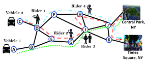
Figure 1: A schematic to illustrate the ride-sharing routing in a region graph, black consisting of 11 regions, $A$ to $K$. There are four ride requests and two vehicles. The locations of both customers and vehicles are shown in the figure above. Two different possible scenarios to serve the ride requests are shown in the figure and depicted by the dashed-red, dotted-green, and dashed-dotted blue lines. The destination of Rider 1 and Rider 4 is the Central Park, NY, while the destination of Rider 2 and Rider 3 is Times Square, NY.

Figure 1 presents an example depicting a real-life scenario. Consider the scenario shown in Figure 1, where Rider 1 and Rider 4 want to go to the Times Squares, NY, while Rider 2, and Rider 3 want to go to the Central Park, NY. The locations of the four customers are depicted in the figure. Also, there are two vehicles located at node (zone) $A$ and node $C$. Without loss of generality, we assume the capacity of the vehicle ($2$) at location $C$ is $5$ passengers while that at location $A$ ($1$) is limited to $4$ passengers only. Given the two vehicles, there is more than one way to serve the requests. Two different possibilities are shown in the figure, assuming ride-sharing is possible. The two of the many possibilities are: (i) serving all the ride requests using only the vehicle $2$, depicted by the dashed-red line in the figure, (ii) serving Rider 1 and Rider 4 using the vehicle $2$ (see the dashed-dotted blue line), while Rider $2$ and Rider $3$ are served using the vehicle $1$(see the dotted-green line).

If ride-sharing is not allowed, only two ride requests among the four can get served at a given time. For example, vehicle $2$ needs to pick up and dispatch rider $1$ first, then, it can pick up rider $4$. Though rider $4$’s location is inside the route of the rider $1$s source and destination. Hence, using ride-sharing, fewer resources (only one vehicle, at location $C$, out of the two) are used and consequently less fuel and emission are consumed [21]. Further, the payment cost per rider should be lower because of sharing the cost among all riders. Besides, ride-sharing reduces traffic congestion and vehicle emission by better utilizing the vehicle seats. Thus, ride-sharing will bring benefits to the driver, riders, and society.

II-B Multi-Hop Delivery for Goods

In Figure 2, a good request is to go from zone C to the destination. The good can be transported by one vehicle from C to B, and another vehicle from B to the destination. Zone B will serve as a transit location referred to in this paper as a “hop-zone”. This flexibility of changing vehicle is multi-hop transport of goods. Such multi-hop flexibility improves the packing of the goods, as was shown for the case of passengers in [20]. For passenger transfers, it was shown that the multi-hop transfers leads to 30% lower cost and 20% more efficient utilization of fleets, as compared to the ride-sharing algorithms. Even though such transfers may not be convenient for passengers, they can be used for the goods which motivates the choice in this paper.

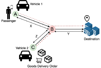
Figure 2: An illustration of multi-hop transportation scenario with hybrid delivery workload. Vehicle 1 and 2 are in zones A and C respectively. Zone B represents a hop-zone’ where the packages part of the goods order packages transfer over to another vehicle

II-C FlexPool Framework

In our proposed framework, we consider an environment with both passenger & goods pick-up requests where vehicles are capable of carrying both types of pick-ups simultaneously. We let vehicle capacity be represented by $C=(C_{p},C_{k})$, where $C_{p}$ is passenger carrying capacity and $C_{k}$ is goods carrying capacity. Integrating the multi-hop goods delivery and ride-sharing services can minimize the total distance travelled while improving the number of requests (passengers & goods both) by the vehicles. Packages can be picked up and dropped off from hop-zones, while passengers will be seated from the point they are picked up till the point they are dropped off. Given such a scenario, assignments will be done to vehicles in a first come first serve manner regardless of package or passenger under the defined capacity constraints.

To illustrate the FlexPool framework, we consider one package and one goods delivery request as depicted in Figure 2. Both the passenger & goods order (set of packages) are to be dropped off at the same destination, while are requested from zones A and C, respectively. Given zone B lies along the delivery route of both requests, Zone B can serve as a transit location. In this scenario, one vehicle (say Vehicle 2) can drop its packages to consequently be picked by another vehicle (Vehicle 1) to deliver to the final destination. Accordingly, the passenger initially gets picked up by the nearest vehicle (Vehicle 1) and the packages by Vehicle 2. Vehicle 2 drops the packages at hop zone B. As Vehicle 1 reaches the hop-zone (Zone B), it picks up the packages and drops both passengers and packages at their destination. As shown in the figure 2, X represents the distance between Zone C and Zone B, Y represents the distance between Zone B and the destination, and Z is the distance between Zone A and Zone C. We define the effective distance traveled by Vehicle 1 ($D_{1}$) by the following equation:

$$D_{1}=\frac{X+Y+Y}{X+Y}=1+\frac{Y}{X+Y}$$ (1)

Effective distance is formally defined as the ratio of total distance covered if no hoping and sharing was allowed to the total distance covered when hoping and sharing is allowed. The efficient packing of vehicles decreases the overall distance traveled by the vehicles in completing service of the same number of requests. The multi-hop scenario shown in Figure 2 reduces the traffic that goes from Zone B to the final destination. Additionally, the accept rate of pick-up requests can be improved as vehicles get assigned more frequently. As in our example Vehicle 1 is free after dropping Package 1 and can pick-up new orders accordingly. We note that the ride-sharing of passengers, multi-hop ride-sharing of goods, as well as joint packing of passengers and goods, decrease the effective distance of vehicles.

II-D Model Parameters and Notations

In this section, we will describe the notations used to represent, the state, action, and reward spaces. The optimization of the system is achieved over $T$ time steps with each step of length $\Delta t$. The fleet make decisions on where on the map to go to serve at each time step $\tau=t_{0},t_{0}+\Delta t,t_{0}+2(\Delta t),\ldots,t_{0}+T(\Delta t)$ where $t_{0}$ is the start time.

The map is split up into a grid with each square being taken as a zone. Zones are represented by $i\in\{1,2,3,\ldots,M\}$. The number of vehicles in the fleet is represented by $N$. A vehicle is marked as available if there is remaining seating or trunk capacity. Vehicles that are completely full or are not considering taking passengers or goods are marked unavailable. Available vehicles in zone $i$ at time slot $t$ is denoted $v_{t,i}$. Only available vehicles are eligible to be dispatched.

$X_{t}$ tracks the vehicle seating capacity and trunk space for packages, denoted as $C_{p,v}$ and $C_{k,v}$, respectively. As a result $X_{t}$ will track: 1. current zone for vehicle $v$, 2. available seats, 3. available trunk space, 4. time at which delivery order is picked up, and 5. destination zone of each delivery order.

Pick-up requests at a given zone $i$ are denoted by $\delta_{t,i}$ at time slot $t$. This represents the demand at a given area at that time. At each time slot $t$, the supply of vehicles for each zone is projected to future time $\tilde{t}$. Consequently, the number of vehicles that will become available at $\tilde{t}$ is denoted by $\delta_{t,\tilde{t},i}$. This value is ascertained from an ETA (estimated time of arrival) prediction for all moving vehicles. Consequently, given a set of dispatch actions, we are able to predict the number of vehicles in each zone for $T$ time slots ahead, denoted by $V_{t:T}$. The pick-up request demand in each zone is predicted through a historical distribution of trips across the zones, and is denoted by $D_{t:T}=(\overline{d}_{t},\ldots,\overline{d}_{t+T})$ from time $t$ to $t+T$. All the data is combined to represent the environment state space $s_{t}$ by the tuple $(X_{t},V_{t:T},D_{t:T})$. At each assignment of a request to vehicle, the state space tuple is updated with the expected pick-up time, source, and destination data.

III FlexPool Framework and Proposed Algorithm

This section presents our distributed framework and the proposed algorithm to train each vehicle in the fleet, which we refer to as an agent, to learn the optimal policy. We will first describe the objectives, and then describe the dispatch and matching policies. The dispatch policy sends unassigned or idle vehicles to regions of anticipated future demand in order to pick up future requests. The matching policy assigns vehicles to pickup nearby requests after the vehicles are dispatched. These will then be combined to provide the overall algorithm.

III-A Objectives for the Proposed Problem

The goals of the Flexpool framework include: (i) satisfying the demand of pick-up orders, thereby minimizing the demand-supply mismatch, (ii) minimizing the time taken to pick-up an order (aka pick-up wait time) in tandem to the dispatch time taken for a vehicle to move to a pick-up location, (iii) minimizing the additional travel time incurred by orders due to participating in a shared vehicle, (iv) minimizing the additional travel time incurred by orders due to layovers at a hop-zone, and (v) minimizing the number of vehicles deployed to minimize fuel consumption and traffic congestion while maximizing utility of available capacity within the available vehicles. These five objectives are studied through the five components, described below. The first component aims to minimize the gap between the supply and demand of order pick-ups. Equation (2) represents this with $v_{t,i}$ is the number of vehicles at time $t$ in zone $i$. Hence we have the supply demand difference accounted for each time slot $t$ at each zone $i$ given by $(\bar{d}_{t,i}-v_{t,i})$

$$\text{diff}_{t}^{(D)}=\sum_{i=1}^{M}(\bar{d}_{t,i}-v_{t,i})^{+}$$ (2)

where $(\cdot)^{+}=\max(0,\cdot)$.

The second component aims to minimize the dispatch time for each vehicle, i.e., time taken for a vehicle to travel current zone from to a zone where pick-ups are made. Available vehicles may be dispatched in two cases: (i) Serve a new request, or (ii) move to locations where a future demand is anticipated. In equation (3), $h_{t,j}^{n}$ represents the estimated travel time for vehicle $n$ to arrive at zone $j$ at time $t$. For all vehicles available within time $t$, we seek to minimize the total dispatch time $T_{t}^{(D)}$,

$$T_{t}^{(D)}=\sum_{n=1}^{N}\sum_{j=1}^{M}h_{t,j}^{n}u_{t,j}^{n}$$ (3)

where $u_{t,j}^{n}=1$ only if vehicle $n$ is dispatched to zone $j$ at time $t$ and $0$ if otherwise. Minimizing dispatch time ultimately minimizes fuel costs when a vehicle is gaining revenue by serving customers.

The third component minimizes the extra travel time for every order (both passengers and packages) that is incurred due to vehicle sharing. For each vehicle $n$ which is carrying $l$ delivery orders of any given kind at each time step $t$, we minimize $\delta_{t,n,l}=t^{{}^{\prime}}+t_{t,n,l}^{\left(a\right)}-t_{n,l)}^{\left(m\right)}$, where $t_{t,n,l}^{\left(a\right)}$ is the updated time the vehicle will take to drop-off passenger/package $l$ due to a change in route and/or addition of another order at time $t$.

$t_{n,l}^{(m)}$ is the travel time that would have been taken if the picked up order $l$ would have travelled without sharing the vehicle with other orders. $t^{{}^{\prime}}$ is the time elapsed after order $l$ was put in the request queue. Equation 4 takes all the above into consideration. The following component expresses, $\Delta_{t}$, the total extra travel overhead time:

$$\Delta_{t}=\sum_{n=1}^{N}\sum_{l=1}^{U_{n}}\delta_{t,n,l}$$ (4)

Note that a given vehicle $n$ may not know the destination of the picked up order. As a results, it will take the expected time of order’s travel generated in any region. Hence, $\delta_{t,n,l}$ is assumed to be the mean value. To minimize the inconvenience of transferring packages at hop-zones to passengers currently being served in a vehicle as well as potential delay in delivery of packages, we introduced the following component which minimizes the number of hops packages are made to go through before being a delivery is fulfilled. Here we define $g$ as the number of packages being carried by a vehicle. $\text{hop}_{g,i,p}$ denotes that package $g$ has undergone a hop-transfer at zone $i$, and $p$ denotes the $p^{\text{th}}$ time the package is being transferred along its journey which is defines as follows:

$$H_{t}=\sum_{i=1}^{M}\sum_{p=1}^{P}\text{hop}_{g,i,p}$$ (5)

Equation (5) provides a sum total of all hop-transfers of all packages being delivered at time step $t$.

The final component aims to minimize the number of vehicles in the fleet. To achieve this, we minimize $e_{t}$ which is indicative of the total vehicles being used at time step $t$. The number of vehicles being used at tine $t$ is given as follows:

$$e_{t}=\sum_{n=1}^{N}\max(e_{t,n}-e_{t-1,n},0)$$ (6)

In equation (6), $e_{t,n}$ indicates whether a vehicle is active. By minimizing the number of fleet vehicle deployed on the roads, we achieve a better utilization per resource. This also results in a reduction of idle cruising time which in turn mitigates extraneous fuel consumption.

The overall objective is a linear combination of all the above described components as follows:

$$\overline{r}=-[\beta_{1}\text{diff}_{t}^{(D)}+\beta_{2}T_{t}^{(D)}+\beta_{3}\Delta_{t}+\beta_{4}e_{t}+\beta_{5}H_{t}],$$ (7)

where the minus sign in the above indicates we want to minimize these terms.

III-B Distributed Dispatch Framework

In this subsection, we describe the distributed framework for dispatch of idle vehicles. For the dispatch, we utilize a reinforcement learning framework, with which we can learn the probabilistic dependence between vehicle actions and the reward function thereby optimizing our objective function as in [18, 19, 20]. In the following, we describe the state, action, and reward for the dispatch policy.

State: The state variables defined in this framework capture the environment status and thus influence the reward feedback to the agents’ actions. We discretize the map of our urban area into a grid of length $\boldsymbol{x}$ and height $\boldsymbol{y}$; resulting a total of $\boldsymbol{x}*\boldsymbol{y}$ zones. This discretization prevents our state and action space from exploding thereby making implementation feasible. The state at time $t$ is captured by following tuple: $(X_{t},V_{t:T},D_{t:T})$. These elements are combined and represented in one vector denoted as $s_{t}$. When a set of new ride requests are generated, the FlexPool engine updates its own data to keep track the environment status. The three-tuple state variables in $s_{t}$ are passed as an input to the DQN input layer which consequently outputs the best action to be taken.

1. $X_{t}$ will track vehicle seating capacity and trunk space for goods/packages. $C_{p,v}$ and $C_{k,v}$ respectively. As a result $X_{t}$ will track: current zone of vehicle $v$, available seats, available trunk space, pick-up time of delivery order, destination zone of each order.

2. $V_{t:T}$ is a prediction of number of available vehicles at each zone for $T$ time slots ahead.

3. $D_{t:T}$ has a term $\delta_{t:T}$ that predicts joint demand of passengers & goods delivery orders at each zone for $T$ time slots ahead.

Action: The action of vehicle $n$ is denoted by $a_{t,n}$ which consists of two components: 1. if the vehicle is partially filled, it decides whether to serve the existing customers (passengers or goods) or to accept new requests, and 2. if it decides to serve a new request or the vehicle is totally empty, it decides the zone it should be dispatched to at time slot t. If vehicle $n$ is full it can not serve any additional customer. Alternatively, if a vehicle decides to serve current customers, the shortest route is used along the road network to pickup the assigned orders.

Reward: Below is the reward function $r_{t,n}=r(s_{t,n},a_{t,n})$ which is used at each agent $n$ of the distributed system at time $t$. The weights shown in equation (8) are used only in instances when an agent is not fully occupied and is eligible to pickup additional orders.

$$\begin{split}r_{t,n}&=\beta_{1}(b_{t,n}+p_{t,n})-\beta_{2}c_{t,n}-\beta_{3}\sum_{u=1}^{U_{n}}\omega_{u}\delta_{t,n,u}\\ &\text{ }-\beta_{4}\max(e_{t,n}-e_{t-1,n},0)-\beta_{5}\max_{u\in\mathcal{L}_{t,n}}H_{u}\end{split}$$ (8)

Here, $b_{t,n}$ denotes the number of passengers served by vehicle $n$ at time $t$ and $p_{t,n}$ denotes the number of packages being carried in the trunk of vehicle $n$ at time $t$. The $\beta_{1}$ term rewards agents for picking up more requests to meet demands.

$c_{t,n}$ denotes the time taken by vehicle $n$ at time $t$ to hop or take detours to pick up extra orders. This term discourages the agent from picking up additional orders without considering the delay in current passengers/goods orders. As a result, the $\beta_{2}$ term prevents adverse effects on customer travel time due to ridesharing.

Further, $\sum_{u=1}^{U_{n}}\omega_{u}\cdot\delta_{t,n,u}$ denotes the sum of additional time vehicle $n$ is incurring at time $t$ to serve additional passengers or packages. The $\omega_{u}$ term is an “urgency” weight for the $u$’th order. This is an attribute assigned based on the type of request (passenger or good) being transported. Ride-sharing passenger requests may be assigned $\omega=1$, whereas goods may be assigned $\omega<1$ since their travel is not as affected by urgency or convenience. Overall, this component penalizes the agent for decisions that delay the transportation of passengers. As a result, agents are incentivized through the $\beta_{4}$ term to prevent loss of customer convenience.

$\max(e_{t,n}-e_{t-1,n},0)$ addresses the objective of minimizing the number of vehicles at $t$ to improve vehicle utilization. Minimizing the $\beta_{4}$ term reduces overall fuel consumption of the fleet.

$\max_{u\in\mathcal{L}_{t,n}}H_{u}$ is the max of the number of hops done by packages in a given vehicle. The $\beta_{5}$ term as a result incentivizing agents to drop-off packages that have been through hop-zones to their final destination, thereby minimizing the number of hops taken by packages.

This reward function is a distributed version of the global objective in (7). With reinforcement learning, we build a representation of the environment at each time step $t$ by a state $s_{t}$ and reward $r_{t}$. Using this information, an action $a_{t}$ is chosen to direct (dispatch) available vehicles to different locations such that the expected discounted future reward, $\sum_{k=t}^{\infty}\eta^{k-t}r(a_{t},s_{t})$, is maximized, where $\eta<1$ is a discount factor.

Algorithm 1 Assign Hop-zone

1:Inputs: Initial Request (Origin, Destination)

2:Outputs: Hop-trips

3:Initialize Hop-trips as a set: [(Origin, Destination)]

4:for trip in Hop-trips do

5:     Compute original delivery distance (Origin to Destination)

6:     Compute distances from Origin to Hop-zones

7:     Assign Hop-zone as the nearest Hop-zone

8:     Compute total delivery distance (Origin to nearest hop-zone to Destination)

9:     if total delivery distance $>2*$original delivery distance then

10:         Return Hop-trips

11:     else

12:         Update Hop-trips as [(Origin, Hop-zone), (Hop-zone, Destination)]

13:         for trip in Hop-trips do

14:              Update Hop-trips using algorithm 1               

15:Return Hop-trips

III-C Hop-zone Designation

As previously mentioned, a hop-zone is a location where a package is dropped off in transit during its journey to its destination. In our algorithm, only goods are assigned hop-zones. Hop-zones are pre-determined locations on the map and are assumed to have the necessary storage infrastructure to hold a large number of packages. As proposed in [8] and [9], POI locations such as gas stations and convenience stores may be incentivized to offer storage services to the transportation system to enable such an infrastructure.

We use a heuristic approach to assign hop-zones to goods delivery requests as shown in Algorithm 1. For each request, we find the nearest hop-zone such that the total delivery distance is less than two times the original distance. If such a hop-zone exists, the trip is split up recursively into hop-trips until no suitable hop-zone assignment can be made upon which the package is delivered to its final destination.

III-D Matching Algorithm

Given the hop-zone locations decided, and the dispatch algorithm using DDQN, we now describe the matching algorithm, detailed in Algorithm 2, for the passengers and goods to each vehicle. As seen in lines 1 and 2 of Algorithm 2, the inputs for the matching algorithm are vehicle status variable $X_{t}$ and the set of requests within a given time-step. The matching algorithm matches the pick-up requests to the vehicle in a greedy fashion minimizing the waiting time of passengers or goods. As seen in lines 3 to 5 of Algorithm 2, we consider all vehicles present within the region where a request is submitted and calculate the ETA, available seating capacity, and available trunk capacity. In Lines 7-10 of Algorithm 2, if the request is a passenger, it is assigned to the nearest vehicle with vacant seats. Whereas if the request is a goods package, it is assigned to the nearest vehicle with vacant trunk space. We note that the matching for the goods and passengers are done in parallel, and if a passenger/good is assigned to multiple vehicles, one is chosen uniformly at random. This maintains the distributed nature of the algorithm. As a result, greedy allocation of passengers and packages are done until either there are no more requests to be assigned or all available vehicles have been fully occupied.

Algorithm 2 Matching Algorithm

1:Inputs: Demand $D_{t}$,Vehicle State Variable $x_{t,n}$,

2:Outputs: Vehicle to Request Assignments

3:if no available requests within reject radius then

4:     Return None

5:Sort requests in ascending order by ETA to pickup location

6:for each request within reject radius of pickup do

7:     if request is passenger then

8:         Calculate remaining seating capacity $C_{p,n}$

9:         if $C_{p,n}>0$ then

10:              Assign passenger to seat

11:         else

12:              Continue          

13:     else if request is goods then

14:         Calculate remaining trunk capacity $C_{k,n}$

15:         if $C_{k,n}>0$ then

16:              Assign package to trunk

17:         else

18:              Continue               

19:Return Vehicle to Request Assignments

Algorithm 3 Double Deep Q-learning with experience replay

1:Initialize replay memory $D$, Q-network parameter $\theta$, and target Q-network $\theta^{-}$.

2:for $e:1:Episodes$ do

3:     Initialize the simulation with arbitrary number of vehicles and ride requests based on real data.

4:     for $t:\Delta t:T$ do

5:         Perform the dispatch and match order

6:         Update the state vector $\varOmega_{t}=$ $(X_{t},V_{t:T},D_{t:T})$.

7:         Update the reward $r_{t}$ based on actions $a_{t}$.

8:         for all available vehicles $n$ do

9:              Create $\varOmega_{t,n}=$ $(X_{t,n},V_{t:T},D_{t:T})$.

10:              Store transition

11:              $(\varOmega_{t-1,n},a_{t-1,n},r_{t,n},\varOmega_{t,n},c_{t,n})$          

12:         Sample random transitions

13:         $(\varOmega_{i},a_{i},r_{i},\varOmega_{i+1},c_{i+1})$ from $D$.

14:         Set $a_{i}^{*}=\text{argmax}_{a^{{}^{\prime}}}Q(\varOmega_{i+1},a_{i}^{*};\theta^{-})$.

15:         Set $z_{i}=r_{i}+\gamma^{1+c_{i+1}}\hat{Q}(\varOmega_{i+1},a_{i}^{*};\theta^{-})$.

16:         minimize $(z_{i}-Q(\varOmega_{i},a_{i};\theta))$ w.r.t. $\theta$.

17:         Set $\theta=\theta^{-}$ every $N$ steps.

18:         Update the set of available vehicles $A_{t}$

19:         for $n$ in $A_{t}$ do

20:              Create $\varOmega_{t,n}=$ $(X_{t,n},V_{t:T},D_{t:T})$.

21:              Choose, with prob. $\epsilon$, a random action from

22:              $a_{t}^{(n)}$.

23:              Else set $a_{t}^{(n)}=\text{argmax}_{a}Q(\varOmega_{t}^{(n)},a;\theta)$.

24:              Send vehicle $n$ to its destination, based on

25:              $a_{t}^{(n)}$.

26:              Update $\varOmega_{t,n}$.               

III-E Double Deep Q-Learning (DDQN)

For each vehicle $n$, a dispatch decision is taken when the vehicle is idle. This policy is learned from the Double Deep Q-Networks (DDQN) approach described in Algorithm 3. The output of the DDQN is the Q-values corresponding to a discrete set of dispatch actions, while the input is the environment status governed by the vector $\boldsymbol{\varOmega}_{t}$. $\boldsymbol{\varOmega}_{t}$ is defined as the state at any time $t$. Every agent $n$ selects the action that maximizes its reward, i.e., taking the argmax of the DDQN-network output (line 14 of Algorithm 3). The learning starts with zero knowledge and actions are chosen following the epsilon-greedy policy where the agent chooses the action that results in the highest Q-value with probability $1-\epsilon$. Consequently, it selects a random action and gathers more information through exploration at a probability of $\epsilon$. The $\epsilon$ is annealed linearly from 1 to 0.05 over $T_{n}$ steps. This allows the agent to balance exploration with exploitation for rewards. Additionally, we use experience replay to overcome the issue of instability due to nonlinear approximations from the neural-network, and due to correlations between the action-value. Experience replay involves accumulating a replay memory buffer of many episodes which is input to the DDQN. DDQN implements Q-Learning with two neural-network-based value functions. One is the target network which learns during the experience-replay while the other is the Q-network which is copy of the last episode of the target network. These two networks are represented by weights $\theta$ and $\theta^{{}^{\prime}}$ respectively. DDQNs have been proven to be effective means of mitigating Q-value overestimations in [22]. In the DDQN, having two function approximators allows to decouple the process of taking actions and estimating the Q-value. For each update in the DDQN, one set of weights is used to determine the greedy policy and the other to determine its value. The target Q-value at any time step $t$ can be defined as:

$$\boldsymbol{T}_{t}={R}_{t+1}+\gamma Q({S}_{t+1},{argmax}_{a}Q({S}_{t+1},a;\theta_{t});{\theta}^{{}^{\prime}}_{t})$$ (9)

where $\theta_{t}$ is the target network used to determine the greedy policy and ${\theta}^{{}^{\prime}}_{t}$ is the Q-network used to evaluate the value of this policy.

Algorithm 4 FlexPool Algorithm

1:Inputs: Environment State Vector $\Omega_{t}$, Pick-up Requests, Map-based locations.

2:Outputs: Decisions for Matching and Dispatching.

3:Create state vector $\Omega_{t,n}=(X_{t},V_{t:t+T},D_{t:t+T})$

4:Initialize vehicle states $X_{0}$ as location of first N requests.

5:for $t\in T$ do

6:     Fetch all pickup requests at time slot t, $D_{t}$

7:     Fetch all available vehicles at time slot t, $V_{t}$

8:     for each vehicle $V_{n}\in V_{t}$ do

9:         if $x_{t,n}^{status}$ is “Dispatching” then

10:              if $x_{t,n}^{location}==a_{n}$ then

11:                  Update $x_{t,n}^{status}$ to “Dispatched”               

12:         else if $x_{t,n}^{status}$ is “Serving” then

13:              if all requests delivered then:

14:                  Update $x_{t,n}^{status}$ to “Idle”               

15:         else if $x_{t,n}^{status}$ is “Matched” then

16:              if Vehicle arrived at pickup location then:

17:                  Update $x_{t,n}^{status}$ to “Serving”                        

18:         if $x_{t,n}^{status}$ is “Idle” then

19:              Push the state vector $\Omega_{t,n}$ to agent

20:              Get the optimal dispatch action $a_{t,n}$ from Q-network

21:              Update $x_{t,n}^{status}$ to “Dispatching”

22:              Drive to dipatch location $a_{t}$ taking the shortest path          

23:         if $x_{t,n}^{status}$ is “Dispatched” then

24:              for each passenger request $\in D_{t}$ do

25:                  Get passenger matching using Algorithm 2

26:                  Update vehicle seating capacity $C_{p,n}$               

27:              for each goods request $\in D_{t}$ do

28:                  Push goods request to Algorithm 1

29:                  Get hop-zone assignments and hop-trips

30:                  Update $D_{t:t+T}$ with hop-trips

31:                  Get goods matching using Algorithm 2

32:                  Update vehicle trunk capacity $C_{k,n}$               

33:              Update $x_{t,n}^{status}$ to “Matched”

34:              Estimate the dispatch and travel time using ETA model

35:              Update $\delta_{t,n}$ if needed, and generate vehicle trajectory

36:              Update $H_{t,n}$ if needed

37:              Drive to pickup requests and update location               

38:     Update the state vector $\Omega_{t+1}$

III-F FlexPool Algorithm

The overall algorithm is shown as Algorithm 4. The inputs are a state vector $\Omega_{t,n}$, pick-up requests, and map-based locations of vehicles and pick-up requests (line 1 of Algorithm 4). The state vector $\Omega_{t,n}$ is determined by the available vehicles and pickup records which are generated from the passenger-goods dataset described in section IV (line 3 of Algorithm 4). Then, we initialize the number of vehicles and generate some pickup requests in each step based on the dataset (see lines 6-7 of Algorithm 4). Each vehicle can be in five states - “Dispatching”, “Serving”, “Matched”, “Idle”, “Dispatched”. The detailed procedure in each of the states is shown in Algorithm 4. To understand the steps, assume that the vehicle just got empty, in which case it will be marked as “Idle” (line 14). In the idle state, the dispatch decision from Q-network is used, and the vehicle is dispatched to the new location. The status is updated to “Dispatching” (line 18-22). In the “Dispatching” state, the vehicle goes to the dispatch location, and upon reaching the desired location, the status is updated to “Dispatched” (line 9-11). If the vehicle has been dispatched, a matching assignment is done for both passenger and goods requests, which will be based on Algorithm 1 and Algorithm 2 (line 23-37). The vehicle status us set to “Matched,” and the vehicle drives to pickup locations and on route to the patch of pickup and delivery of assigned passengers and goods. The extra travel time $\delta_{t,n}$ and hop counter $H_{t,n}$ are updated as needed (see lines 35-36 of Algorithm 4). If the vehicle has been matched and has crossed the pickup location, it is marked as “Serving” (line 15-17). After all the passengers and goods that were matched have been delivered, the vehicle status changes to “Idle” (line 12-14). The procedure repeats itself going through these stages.

As mentioned previously, the output of the DDQN is the Q-values for each movement possible on the map for a given vehicle. Note that each update is performed in parallel across all agents. Each agent however does not anticipate the actions of other agents on the map thus limiting coordination amongst them. Consequently, the vehicles travel to their chosen dispatch locations by using the shortest path on the road network graph as seen in line 20 of Algorithm 4. It is to be noted that FlexPool can is scalable to a large number of vehicles and requests. The factors that enable these are: 1. each agent solves its own DDQN which runs at a time complexity of O(1) during inference, and 2. the distributed nature of our algorithm allows each vehicle to take a discrete set of actions. This prevents explosion in action space since we do not consider the joint action space across all agents.

IV Simulator Setup

The fleet of autonomous vehicles were trained in a virtual spatio-temporal environment that simulates urban traffic and routing. In our simulator, we used the road network of the New York City Metropolitan area along with a realistic simulation of taxi pick-ups and package delivery requests. This simulator hosts each deep reinforcement learning agent which acts as a delivery vehicle in the New York City area that is looking to maximize its reward.

IV-A Dataset

The delivery workload in this simulator consists of passenger pick-up requests as well as package delivery requests for various goods and services. To emulate a realistic workload of passenger pick-ups in the urban environment, we used the New York City taxi trip data set from [16].We extracted trips within the major burrows of the metropolitan area from May and June for our simulation.

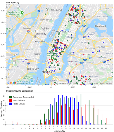
Figure 3: The map and graph show different types of goods delivery requests.

In simulating package delivery requests, customer check-in traffic was extracted from Google Maps for postal service, meal delivery, and supermarket locations. The 100 most active locations were considered from each of the respective service types. Average check-in traffic was extracted for each day of the week for each location. This was used to generate a synthetic workload for a total of two months representative of May and June. Figure 3 shows the distribution of check-ins across the city over a synthetic workload, which was generated from customer check-in from Google Maps analytics data. At each service location, the request rates were generated by Poisson distribution given in equation (10) across request rate $x$, where $\lambda$ represents the observed check-in rate from Google Maps. Consequently, for each service location, package drop-off locations were generated randomly considering delivery radius limit of 5 miles in accordance with the current standard for major crowd-sourced delivery services such as DoorDash and GrubHub. All pick-up and drop-off locations are constrained within the New York City borough boundaries. The resulting data set consisted of goods delivery orders over one month.

$$p(x;\lambda)=\frac{e^{-\lambda}\lambda^{x}}{x!}\\ ;x\in\mathbb{Z}$$ (10)

We let the vehicle carrying capacities be $C_{p}=4$ passengers and $C_{k}=5$ packages, unless stated otherwise. A request is deemed rejected if there are no vehicles available within a radius of $5km^{2}$. When an adequate number of vehicles are not present to meet the demand of pick-up requests, a higher reject rate can be observed.

IV-B Initialization

A directed graph was constructed as the NYC road network from OpenStreetMaps by partitioning the city into a 212 x 219 service area grid of size 150m x 150m each. In performing routing, pick-up and drop-off locations are snipped to the closest edge-nodes of the network and a shortest path algorithm is found to estimate the travel times. To estimate the minimal travel time for each dispatch, the travel time between every two dispatch nodes/location is ascertained. Every third intersection of zones in the horizontal and vertical direction is considered a hop-zone. To allow hop-zones to be adequate transit locations for the majority of the rides, we ensure that the hop-zones are in the busy area of the city and are not too closely placed. As a result, there were a total of 195 hop-zone candidates. To further eliminate under-utilized hop-zones, we consider only the zones with at least 10 pick-up requests in the day. Consequently, we obtain a total of 148 hop-zones in the urban simulation.

To initialize the environment, we run the simulation for 100 iterations without dispatching vehicles. At default setting, the simulator initializes 8000 vehicles unless specified otherwise. The maximum horizon is defined as $T=30$ steps where $\Delta T=1$minute. Unless otherwise stated, the reward function parameters are set to be the following: $\beta_{1}=10,\beta_{2}=1,\beta_{3}=1,\beta_{4}=0.05$, and $\beta_{5}=2$. We also assign $\omega=1$ for passengers, and $\omega=0.5$ for goods to emphasize the minimizing passenger delays. The algorithm also needs estimate of Estimated Time of Arrival (ETA) and Demand prediction. These estimates are based on deep learning framework and follow the procedure as in [19]. The details are also provided in Appendix A for completeness.

IV-C DDQN Implementation

Each agent is trained using a Double Deep Q-Network (DDQN) algorithm. The dispatch action space of a given agent is limited to 7 grid boxes vertically and horizontally. To achieve this, the New York City area map was divided into $41\times 43$ grids. As a result, each vehicle is able to make a decision on what part of the map to move to pick-up orders within the $15\times 15$ grid around its current location. The DDQN takes the state space tuple previously defined as its input. This includes the state of vehicles, supply, and demand. We feed the predicted requests in the next 15 minutes obtained from the demand model, the current location of each vehicle, and snapshots of vehicle location in the next 15, and 30 minutes. The network architecture of the DDQN consists of 16 convolution layers of $5\times 5$, 32 convolution layer of $3\times 3$, 64 convolution layer of $3\times 3$, 16 convolution layer of $1\times 1$. All convolution layers have a ReLu activation. The output of the deep Q network is an array of $15\times 15$ Q values. Each value corresponds to the discounted sum of rewards a vehicle could get if dispatched to that particular zone. As previously explained, Algorithm 4 shows detailed steps on how the FlexPool works.

In training this Q-network, we face the challenge of learning instability that is generally associated with Reinforcement Learning which uses rich function approximators such as Neural Networks. To combat this, we use experience replay and fixed Q-targets. This requires us to keep two sets of networks: the target network and the Q-network. The target network is what is ultimately used to generate the Q-values. The weights for the target network is periodically updated using the Q-network at an interval of 150 iterations. The Q-network on the other hand is learned at each iteration using a replay buffer of 10,000 steps.

Given the distributed nature of our algorithm, every vehicle runs its own DDQN policy. As a result, the environment during training changes over time from the perspective of individual vehicles. To mitigate such effects, a new parameter $\beta$ is imposed to give the probability of performing an action in each time step. In our training procedure, $\beta$ is increased linearly from 0.3 to 1.0 over the first $T_{n}$ steps where $n$ is the number of vehicles. This allows only 30% of the vehicles takes an actions at the onset. Consequently, the number of vehicles moving in each time step does not fluctuate significantly as our DDQN approaches the optimal policy.

Training is performed using a total of 22,500 iterations, consisting of 30 episodes of 750 iterations each. Each iteration consists of 750 minutes of data, which is equivalent to two weeks data. The average q-max curve of all agents combined is plotted in figure 4. With the particular experiment shown in Figure 4, we initialized a fleet of $n=8000$ vehicles. The DDQN parameters included a start exploration rate $\epsilon=1$ which was linearly decayed for $T_{n}$ steps which in this instance is 8000 steps.

It can be observed from the learning curve that over the first $T_{n}$ steps there is a gradual increase in the average Q-max of the fleet. This is explainable as it is within the exploration phase where the agents are gradually zeroing in on optimal policy. The average Q-max values hit a peak at 8000 steps and drop slightly as $\beta\to 1$. At this phase, all the agents are taking actions and competing for pick-ups, hence the average Q-max decreases until convergence at around 15,000 steps. In the experiment shown, the average Q-max converges at a value of approximately 35.

We trained the DDQN agents in our simulation for a total of one month using all dataset requests from May. Consequently, we evaluated these trained DDQN agents by simulating two additional weeks from the month of June.

Figure 4: This plot shows the convergence of Q-values during training. We see convergence in approximately 15,000 training steps.

V Evaluation and Results

In this section, we will evaluate the proposed approach, labeled as FlexPool w/ Hoptrips. We choose the parameters as $C_{p}=4$, $C_{k}=5$, $\beta_{1}=10$, $\beta_{2}=1$, $\beta_{3}=0.5$, $\beta_{4}=1$, and $\beta_{5}=1$, unless explicitly mentioned. We compare the proposed algorithm with two baselines as described below.

1. FlexPool w/o Hoptrips: This baseline involves combined workloads for agents without hoptrips. In this case, goods packages are delivered directly from pick-up to drop-off locations without transit. Since there are no hop-trips, $\beta_{5}=0$.

2. Separate Vehicles: This baseline is analogous to DeepPool [19], where passengers & goods are pooled into separate sets of vehicles. Vehicle for passenger pick-ups is designated as ride-sharing vehicles with max capacity $C_{p}=4$ assuming 4 seats in a car. Vehicles assigned to packages are designated as goods fulfillment vehicles with a max capacity $C_{k}=10$ since we assume the entire car capacity (seats+trunk) can be used for goods. All other parameters are as in FlexPool w/o Hoptrips.

Figure 5: This figure plots Accept Rates of all pick-up requests (passengers & goods) for each of the 14 test days for all three models. We see that all three models accept above 90% of all requests.

Figure 6: This figure plots Accept Rates of passenger rideshare requests for each of the 14 test days for all three models. We see that all three models accept above 90% of passenger rideshare requests.

Figure 7: This figure plots Accept Rates of goods delivery requests for each of the 14 test days for all three models. We see that all three models accept above 90% of goods delivery requests.

V-A Evaluated Metrics

For each of the considered algorithms, we evaluate the following metrics and outline their significance to the joint passenger and goods problem:

• Accept Rate: Accept rate is defined as the ratio of successful pick-ups by the fleet to the total number of requests made to the fleet in a given time slot. A high accept rate is a characteristic of a reliable mode of transportation. With a high accept rate, our fleet is able to fulfill the transportation demands for passenger and/or goods.

• Fuel Cost per Delivery: This is defined as the ratio of total fuel consumption by the fleet to the number of requests fulfilled by the fleet. The following assumptions are made in estimating cost: 1. $2 (USD) per US gallon which is a ballpark estimate of US fuel prices as per [23], and 2. Each vehicle in the fleet consumes 0.5 US gallons per hour of driving. With a smaller amount of time a fleet vehicle spends traveling per request, less fuel is consumed which reduces congestion and emissions. A good performance on this metric, therefore, points towards a better overall transportation system efficiency.

• Active Vehicles Ratio: The vehicles deployed from the fleet to serve customer demand are defined as “active vehicles”. We take an average of active vehicles in the fleet over the model evaluation duration. As defined in our reward in equation (6), the objective of the fleet is to minimize the number of vehicles deployed on the road. By minimizing the number of active vehicles, we achieve better utilization of individual vehicles in serving the demand. Given that (i) all baselines are catering to a similar volume of pickup orders, and (ii) all baselines are achieving a similar accept rate, a lower Active Vehicles Ratio indicates that a fleet is able to minimize the number of vehicles on the street to serve the requests.

• Wait time: This is the time taken for a passenger or goods delivery request to be picked up by the fleet. We note that wait time is an important metric for customer convenience with mobility-on-demand services. A low wait time as a result is ideal for both passengers and goods.

• Effective Distance Ratio: This is defined as the ratio of total distance covered if no multi-hops and sharing are allowed to the total distance covered when multi-hop and sharing is allowed. The efficient packing of vehicles alleviates the overall distance traveled by the vehicles in completing service for the same number of requests. Ride-sharing for passengers and multi-hop transport of goods reduces the effective distance of the vehicles due to efficient packing.

Figure 8: This figure plots Fuel Cost per Delivery with varying fleet size for all three models. We see that for all fleet sizes, FlexPool w/ Hoptrips has the lowest fuel cost in fulfilling requests.

Figure 9: This figure plots Active Vehicles Ratio with varying fleet size for all three models. We see that for all fleet sizes, FlexPool w/ Hoptrips achieves the lowest Active Vehicles Ratio in comparison to baselines.

Figure 10: This figure plots wait times of all requests for each of the 14 test days for all three models. We see that FlexPool w/ Hoptrips achieves lowest average wait time per pick-up in comparison to the baselines.

Figure 11: This figure plots the effective distance ratio for all three models. We see that the effective distance ratio of FlexPool is significantly larger than the baselines. With fewer fleet vehicles, FlexPool is able to achieve a better effective distance ratio thus achieving better packing of passengers and goods.

V-B Discussion on the Results

In this section, we compare the results obtained from our simulation of our proposed algorithm (FlexPool w/ Hoptrips) against the two baseline scenarios defined previously (FlexPool w/o Hoptrips and Separate Vehicles).

In evaluating accept rates for the three models, we use a fleet size of $n=8000$ vehicles. Figures 7, 7, and 7 show that the three algorithms accept 90% of requests in the worst case with averages of 95%. In accepting passenger ride-share requests, FlexPool w/ hoptrips and FlexPool w/o hoptrips are identical in carrying capacities, however FlexPool w/ hoptrips is able to pick-up passengers at higher rates. In comparing goods delivery order accept rates (see Figure 7), the Separate Vehicles baseline slightly outperforms other models potentially due to greater carrying capacity (both seats and trunk available for carrying goods). From the accept rate results, we observe that all three algorithms are in a similar ballpark. Therefore, we may compare the subsequent metrics to have a fair evaluation of system efficiency and sustainability across the three algorithms.

We evaluate fuel cost per delivery across different fleet sizes for all three algorithms. Figure 10 shows the model performance on this metric. We observe from this plot that the proposed model (FlexPool w/ Hoptrips) clearly outperforms the baselines. With all three algorithms being in the same accept rate ballpark, this plot shows that the proposed model is able to fulfill delivery requests on an average with much lower fuel consumption. This points to cost savings on the part of the fleet operator. Additionally, given our simulator models fuel cost directly using vehicle travel time, a good performance on this metric indicates that vehicles spend less time on the road in fulfilling deliveries. This results in reducing congestion and emissions as well. With an average improvement of  30% from the next best baseline (FlexPool w/o Hoptrips), this goes to show the promise that using a combined workload with hoptrips has from both cost and sustainability standpoints. With both FlexPool models outperforming the separated vehicles model, it is evident that combining passenger & goods workloads into one system is more sustainable and cost-efficient.

In Fig. 11, we observe that the effective distance ratio varies with the number of fleet vehicles. Amongst all three algorithms, it is evident that our proposed algorithm achieves the highest effective distance ratio. This suggests that the vehicles are able to fulfill more deliveries at a given time as a result of being more efficiently packed. The FlexPool w/o Hoptrips baseline performs second best while the Separate Vehicles baseline achieves the lowest effective distance ratio. This can be explained by the ability of FlexPool w/o Hoptrips to better utilize the full capacity of a vehicle (seating space + trunk space), while Separate Vehicles underutilizes trunk space as a result of not considering goods requests while delivering passengers.

In the definition of our global objective (refer to Section III), we included a component to minimize the number of deployed vehicles to serve passenger demand. Having noted that all 3 models achieve similar performance in accept rates for pickups, it is noteworthy that 10 shows a significant improvement in the number of vehicles deployed with the FlexPool w/ Hoptrips. On average FlexPool w/ Hoptrips outperforms the next best baseline by approximately 35%. This points to the higher utilization of fleet vehicles to achieve reliable accept rates.

Figure 10 shows the performance on the wait time of order pick-ups by the models over the test duration. It can be observed that FlexPool w/ hoptrips achieves the lowest time to pick-up orders. As there is a significant improvement in comparison to FlexPool w/o hoptrips, it is fair to infer that the use of a multi-hop routing for packages reduces the waiting time for orders to be picked up. Likewise, both FlexPool models outperform the Separate Vehicles scenario. We note that, when vehicles have the ability to pickup both passengers & goods, requests are more likely to be accepted quickly resulting in improved customer wait times.

VI Conclusions and Future Work

We propose FlexPool as a distributed model-free algorithm for joint ride-sharing of passengers and goods, which uses deep neural networks and reinforcement learning to learn optimal dispatch policies by interacting with the environment and an efficient matching of the passengers and goods to the vehicles. The proposed approach enables pooling of passengers as well as multi-hop transfer of goods, helping efficient use of the vehicles. Through efficiently incorporating passenger and goods delivery demand statistics and deep learning models, our proposed method manages dispatching and matching solutions for an efficient and sustainable combined transportation service. In addressing the problem of joint transportation of passengers and goods workloads, FlexPool is able to achieve a significantly higher operational efficiency as well as a lower environmental footprint. As a distributed system, FlexPool can adapt fluidly to a dynamic environment with fluctuations in demands of different workloads.

FlexPool assumes existing infrastructure to enable convenient storage during multi-hop transit for goods delivery. In practice however, cost efficient methods for goods transit are currently not present and this would be very valuable piece of infrastructure to allow multi-hop transit. Along the same lines, research of practical incentives to encourage multi-hop transfers such as new pricing models would be of great use in enabling this technology. Another important aspect that needs to be explored is the incorporation of deadline based constraints to allow for delivery of urgent goods or service-based pricing contracts with customers. Likewise, a multi-agent formulation involving coordination among vehicles would be an interesting extension to the proposed solution to the shared passengers & goods delivery problem.

VII Acknowledgement

The authors would like to thank Intel for giving us access to the Intel DevCloud cluster for this project. This work was supported in part by DARPA SAIL-ON project “Generating Novelty in Open-world Multi-agent Environments (GNOME)”.

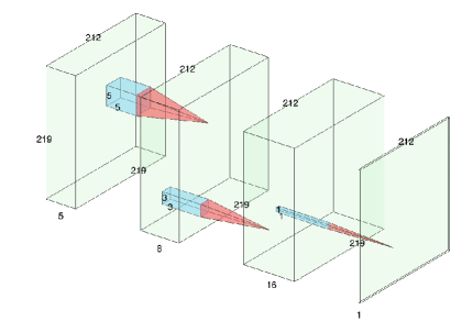
Figure 12: This diagram shows the Conv-Net architecture of the Demand Prediction Model.

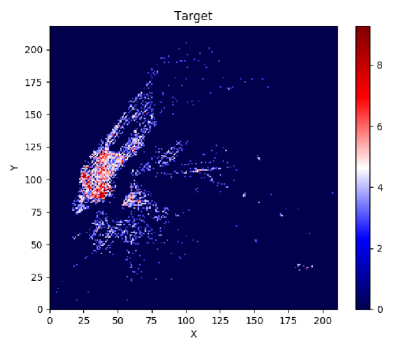
(a) This shows a heatmap of actual demand from the dataset which is used as a target to train the demand prediction model.

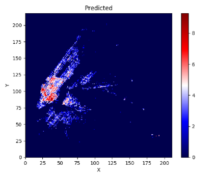
(b) This shows a heatmap obtained from the demand prediction model which predicted pickup demand over the map.

Figure 13: The above heatmaps visualize target and predicted demand areas. Warmer colors indicate a higher demand as shown by the color scale.

Appendix A ETA and Demand Prediction

The simulator uses an Estimated Time of Arrival (ETA) model to predict the estimated trip times. This model is built using the New York City taxi data set. In the ETA model, we want to predict the expected travel time between two zones (two pairs of latitudes and longitudes). We split our data into 70% train and 30% test. We use day of week, latitude, longitude and time of days as the explanatory variables and use random forest to predict the ETA. The final ETA model yielded a root mean squared error (RMSE) of 3.4 on the test data.

The demand prediction model is a critical element to the simulator in building the state space vector that allows DDQN agents to proactively dispatch towards areas where there is a high demand. This model is built using the Conv-Net architecture shown in figure 12. The network outputs a $212\times 219$ heat map image in which each pixel stands for the predicted number of pick-up requests for each location on the map for the following 30 minutes of simulation. The network is fed with input images which represent the actual pick-ups of all service types over the last 6 time-steps. The actual pick-up counts over the map is combined with the sine and cosine of the day of week and hour of day to capture the daily and weekly periodicity of the demand. After training using a 80% train and 20% test split, RMSE values for training and testing were 0.945 and 1.217 respectively. Figure 13 shows the demand heat map of a target sample and a predicted sample of this demand prediction model. The predicted demand in this figure is a sample $212\times 219$ output of the Conv-Net Architecture from Figure 12.

Symbol	Description
$N$	number of vehicles
${v}_{t,i}$	number of available vehicles at time $t$ in map region $i$
${d}_{t,i}$	number of requests at time $t$ in map region $i$
$d_{t,\widetilde{t},i}$	number of additional vehicles anticipated to become available in region $i$ by time $\widetilde{t}$ at time $t$
${x}_{t,n}$	current location for vehicle $n$, current status, available seating, available trunk space, time at which a request is picked up, and destination of each request
$\varOmega_{t,n}$	state of vehicle $n$ at time $t$
${a}_{t,n}$	action of vehicle $n$ at time $t$
$r_{t,n}$	reward of vehicle $n$ at time $t$
$\beta_{i}$	weight of component $i$ in the reward expression
$b_{t,n}$	number of customers served by vehicle $n$ at time $t$
$p_{t,n}$	number of packages being carried by vehicle $n$ at time $t$
$c_{t,n}$	time spent by vehicle $n$ to hop or take a detour to pick up additional requests
$\omega_{u}$	delivery “urgency” weight assigned for the $u$’th request
$\delta_{t,n,u}$	additional driving time spent on delivering request $u$ by vehicle $n$ due to other concurrent deliveries
$e_{t,n}$	occupied flag for vehicle $n$ at time $t$
$H_{u}$	number of “hops” completed by package $u$
$\mathcal{L}_{t,n}$	list of all requests assigned to vehicle $n$ at time $t$

TABLE I: Table of notations used in the paper.

Appendix B Table of Notations

Table I provides the summary of key notations that are used in this paper.

References

- [1] B. Asdecker and F. Zirkelbach, “What drives the drivers? a qualitative perspective on what motivates the crowd delivery workforce,” in Proceedings of the 53rd Hawaii International Conference on System Sciences, 2020.
- [2] S. Arora and A. Verma, “M-commerce: Crusader for “phygital” retail,” M-Commerce: Experiencing the Phygital Retail, p. 163, 2019.
- [3] Y. J. Jo, M. Matsumura, and D. E. Weinstein, “The impact of e-commerce on relative prices and consumer welfare,” tech. rep., National Bureau of Economic Research, 2019.
- [4] N. Bubner, N. Bubner, R. Helfifg, and M. Jeske, “Logistics trend radar,” DHL Trend Research, 2014.
- [5] N. Yaraghi and S. Ravi, “The current and future state of the sharing economy,” Available at SSRN 3041207, 2017.
- [6] R. Hahn and R. Metcalfe, “The ridesharing revolution: Economic survey and synthesis,” More equal by design: economic design responses to inequality, vol. 4, 2017.
- [7] K. Kokalitcheva, “Uber now has 40 million monthly riders worldwide,” Fortune Magazine, 2016.
- [8] C. Chen, D. Zhang, X. Ma, B. Guo, L. Wang, Y. Wang, and E. Sha, “crowddeliver: Planning city-wide package delivery paths leveraging the crowd of taxis,” IEEE Transactions on Intelligent Transportation Systems, vol. 18, no. 6, pp. 1478–1496, 2017.
- [9] C. Chen, Z. Wang, and D. Zhang, “Sending more with less: Crowdsourcing integrated transportation as a new form of citywide passenger–package delivery system,” IT Professional, vol. 22, no. 1, pp. 56–62, 2020.
- [10] N.-Q. Nguyen, N.-V.-D. Nghiem, P.-T. Do, K.-T. LE, M.-S. Nguyen, and N. Mukai, “People and parcels sharing a taxi for tokyo city,” in Proceedings of the Sixth International Symposium on Information and Communication Technology, pp. 90–97, 2015.
- [11] V. Ghilas, E. Demir, and T. Van Woensel, “Integrating passenger and freight transportation: Model formulation and insights,” Proceedings of the 2013 Beta Working Papers (WP), vol. 441, 2013.
- [12] R. Masson, A. Trentini, F. Lehuédé, N. Malhéné, O. Péton, and H. Tlahig, “Optimization of a city logistics transportation system with mixed passengers and goods,” EURO Journal on Transportation and Logistics, vol. 6, no. 1, pp. 81–109, 2017.
- [13] E. Fatnassi, J. Chaouachi, and W. Klibi, “Planning and operating a shared goods and passengers on-demand rapid transit system for sustainable city-logistics,” Transportation Research Part B: Methodological, vol. 81, pp. 440–460, 2015.
- [14] W. Chen, M. Mes, and M. Schutten, “Multi-hop driver-parcel matching problem with time windows,” Flexible services and manufacturing journal, vol. 30, no. 3, pp. 517–553, 2018.
- [15] K. Arulkumaran, M. P. Deisenroth, M. Brundage, and A. A. Bharath, “A brief survey of deep reinforcement learning,” arXiv preprint arXiv:1708.05866, 2017.
- [16] N. Taxi, “Limousine commission-trip record data,” 2018.
- [17] L. Schultz and V. Sokolov, “Deep reinforcement learning for dynamic urban transportation problems,” arXiv preprint arXiv:1806.05310, 2018.
- [18] T. Oda and C. Joe-Wong, “Movi: A model-free approach to dynamic fleet management,” in IEEE INFOCOM 2018-IEEE Conference on Computer Communications, pp. 2708–2716, IEEE, 2018.
- [19] A. O. Al-Abbasi, A. Ghosh, and V. Aggarwal, “Deeppool: Distributed model-free algorithm for ride-sharing using deep reinforcement learning,” IEEE Transactions on Intelligent Transportation Systems, vol. 20, no. 12, pp. 4714–4727, 2019.
- [20] A. Singh, A. Alabbasi, and V. Aggarwal, “A distributed model-free algorithm for multi-hop ride-sharing using deep reinforcement learning,” arXiv preprint arXiv:1910.14002, 2019.
- [21] S. Shaheen, “Shared mobility: the potential of ridehailing and pooling,” in Three Revolutions, pp. 55–76, Springer, 2018.
- [22] H. v. Hasselt, A. Guez, and D. Silver, “Deep reinforcement learning with double q-learning,” in Proceedings of the Thirtieth AAAI Conference on Artificial Intelligence, pp. 2094–2100, 2016.
- [23] AAA, “Us state gas prices.” https://gasprices.aaa.com/state-gas-price-averages/, 2020. Accessed: 2020-01-30.