Using Machine Learning to Identify the Most At-Risk Students in Physics Classes

Abstract

Machine learning algorithms have recently been used to predict students’ performance in an introductory physics class. The prediction model classified students as those likely to receive an A or B or students likely to receive a grade of C, D, F or withdraw from the class. Early prediction could better allow the direction of educational interventions and the allocation of educational resources. However, the performance metrics used in that study become unreliable when used to classify whether a student would receive an A, B or C (the ABC outcome) or if they would receive a D, F or withdraw (W) from the class (the DFW outcome) because the outcome is substantially unbalanced with between 10% to 20% of the students receiving a D, F, or W. This work presents techniques to adjust the prediction models and alternate model performance metrics more appropriate for unbalanced outcome variables. These techniques were applied to three samples drawn from introductory mechanics classes at two institutions ($N=7184$, $1683$, and $926$). Applying the same methods as the earlier study produced a classifier that was very inaccurate, classifying only 16% of the DFW cases correctly; tuning the model increased the DFW classification accuracy to 43%. Using a combination of institutional and in-class data improved DFW accuracy to 53% by the second week of class. As in the prior study, demographic variables such as gender, underrepresented minority status, first-generation college student status, and low socioeconomic status were not important variables in the final prediction models.

I Introduction

Physics courses, along with other core science and mathematics courses, form key hurdles for Science, Technology, Engineering, and Mathematics (STEM) students early in their college career. Student success in these classes is important to improving STEM retention; the success of students traditionally underrepresented in STEM disciplines in the core classes may be a limiting factor in increasing inclusion in STEM fields. Physics Education Research (PER) has developed a wide range of research-based instructional materials and practices to help students learn physics Meltzer and Thornton (2012). Research-based instructional strategies have been demonstrated to increase student success and retention Freeman et al. (2014). While some of these strategies are easily implemented for large classes, others have substantial implementation costs. Further, no class could implement all possible research-based strategies, and some may be more appropriate for some subsets of students than for others. One method to better distribute resources to the students who would benefit the most is to identify at-risk students early in physics classes. The effective identification of students at risk in physics classes and the efficacious uses of this classification represents a promising new research strand in PER.

The need for STEM graduates continues to increase at a rate that is outstripping STEM graduation rates across American institutions. A 2012 report from the President’s Council of Advisors on Science and Technology of Advisors on Science and Technology (2012) identified the need to increase graduation of STEM majors to avoid a projected shortfall of one million STEM job candidates over the next decade. Improving STEM retention has long been an important area of investigation for science education researchers Rask (2010); Chen (2013); Shaw and Barbuti (2010); Maltese and Tai (2011); Zhang et al. (2004); French et al. (2005); Marra et al. (2012); Hall et al. (2015). Targeting interventions to students at risk in core introductory science and mathematics courses taken early in college offers one potential mechanism to improve STEM graduation rates. In recent years, educational data mining has become a prominent method of analyzing student data to inform course redesign and to predict student performance and persistence Baepler and Murdoch (2010); Baker and Yacef (2009); Papamitsiou and Economides (2014); Dutt et al. (2017); Romero and Ventura (2010).

The current study investigates the application of machine learning algorithms to identify at-risk students. Machine learning and data science as a whole are growing explosively in many segments of the economy as these new methods are used to make sense and exploit the exponentially growing data collected in an increasing online world. These methods are also being adapted to understand and improve educational data systems. It seems likely that this process will accelerate in the near future as universities, in a challenging financial climate, attempt to retain as many students as possible. We argue that PER should help shape both the construction of retention models of physics students and explore their most effective and most ethical use. The following summarizes the prior study applying Education Data Mining (EDM) techniques in physics classes, provides an overview of EDM, and more specifically an overview of the use of EDM for grade prediction.

I.1 Prior Study: Study 1

This study extends the results of Zabriskie et al. Zabriskie et al. (2019) which will be referred to as Study 1 in this work. Study 1 used institutional data such as ACT scores and college GPA (CGPA) as well as data collected within a physics class such as homework grades and test scores to predict whether a student would receive an A or B in the first and second semester of a calculus-based physics class at a large university. The study used both logistic regression and random forests to classify students. Random forest classification using only institutional variables was 73% accurate for the first semester class. This accuracy increased to 80% by the fifth week of the class when in-class variables were included. The logistic regression and random forest classification algorithms generated very similar results. Study 1 chose to predict A and B outcomes, rather than the more important A, B, and C outcomes, partially because the sample was significantly unbalanced. Sample imbalance makes classification accuracy more difficult to interpret. Study 1 investigated the effect of a number of demographic variables (gender, underrepresented minority status, and first-generation status) on grade prediction and found they were not important to grade classification. These groups (women, underrepresented minority students, and first-generation students) were very underrepresented in the sample studied; it was unclear to what extent the low importance of the demographic variables was caused by the demographic imbalance of the sample.

I.2 Research Questions

This study seeks to extend the application of machine learning algorithms to predict whether a student will earn a D or F or withdraw (W) from a physics class. In particular, we explore the following research questions:

1. How can machine learning algorithms be applied to predict an unbalanced outcome in a physics class?

2. Does classification accuracy differ for underrepresented groups in physics? If so, how and why does it differ?

3. How can the results of a machine learning analysis be applied to better understand and improve physics instruction?

I.3 Educational Data Mining

Educational Data Mining (EDM) can be described as the use of statistical, machine learning, and traditional data mining methods to draw conclusions from large educational datasets while incorporating predictive modeling and psychometric modeling Romero and Ventura (2010). In a 2014 meta-analysis of 240 EDM articles by Peña-Ayala, 88% of the studies were found to use a statistical and/or machine learning approach to draw conclusions from the data presented. Of these studies, 22% analyzed student behavior, 21% examined student performance, and 20% examined assessments Peña-Ayala (2014). Peña-Ayala also found that classification was the most common method used in EDM applied in 42% of all analyses, with clustering used in 27%, and regression used in 15% of studies.

Educational Data Mining encompasses a large number of statistical and machine learning techniques with logistic regression, decision trees, random forests, neural networks, naive Bayes, support vector machines, and K-nearest neighbor algorithms commonly applied Romero et al. (2008). Peña-Ayala’s Peña-Ayala (2014) analysis found 20% of studies employed Bayes theorem and 18% decision trees. Decision trees and random forests are one of the more commonly used techniques in EDM. We use these techniques to investigate our research questions and explore ways to assess the success of machine learning algorithms. More information on the fundamentals of these and other machine learning techniques are readily available through a number of machine learning texts James et al. (2017); Müller and Guido (2016).

I.4 Grade Prediction and Persistence

While EDM is used for a wide array of purposes, it has often been used to examine student performance and persistence. One survey by Shahiri et al. summarized 30 studies in which student performance was examined using EDM techniques Shahiri et al. (2015). Neural networks and decision trees were the two most common techniques used in studies examining student performance with naive Bayes, K-nearest neighbors, and support vector machines used in some studies. A study by Huang and Fang examined student performance on the final exam for a large-enrollment engineering course using measurements of college GPA, performance in 3 prerequisite math classes as well as Physics 1, and student performance on in-semester examinations Huang and Fang (2013). They analyzed the data using a large number of techniques commonly used in EDM and found relatively little difference in the accuracy of the resulting models. Study 1 also found little difference in the performance of machine learning algorithms in predicting physics grades. Another study examining an introductory engineering course by Marbouti et al. used an array of EDM techniques to predict student grade outcomes of C or better Marbouti et al. (2016). They used in-class measures of student performance including homework, quiz, and exam 1 scores and found that logistic regression provided the highest accuracy at 94%. A study by Macfadyen and Dawson attempted to identify students at risk of failure in an introductory biology course Macfadyen and Dawson (2010). Using logistic regression they were able to identify students failing (defined as having a grade of less than $50\%$) with 81% accuracy. With the goal of improving STEM retention, many universities are taking a rising interest in using EDM techniques for grade and persistence prediction in STEM classes bin Mat et al. (2013).

The use of machine learning techniques in physics classes has only begun recently. In addition to Study 1, random forests were used in a 2018 study by Aiken et al. to predict student persistence as physics majors and identify the factors that are predictive of students either remaining physics majors or becoming engineering majors Aiken et al. (2019).

II Methods

Table 1: Full list of variables.

Variable	Sample			Type	Description
	1	2	3
Institutional Variables
Gender	$\times$	$\times$	$\times$	Dichotomous	Does the student identify as a man or a women?
URM	$\times$	$\times$	$\times$	Dichotomous	Does the student identify as an underrepresented minority?
FirstGen	$\times$	$\times$	$\times$	Dichotomous	Is the student a first-generation college student?
CalReady	$\times$	$\times$		Dichotomous	Is the student ready for calculus?
SES			$\times$	Dichotomous	Does the student qualify for a Pell grant?
CmpPct	$\times$	$\times$		Continuous	Percentage of credit hours attempted that were completed.
CGPA	$\times$	$\times$	$\times$	Continuous	College GPA at the start of the course.
STEMCls	$\times$	$\times$		Continuous	Number of STEM classes completed at the start of the course.
HrsCmp	$\times$	$\times$		Continuous	Total credits hours earned at the start of the course.
HrsEnroll	$\times$	$\times$		Continuous	Current credits hours enrolled at the start of the course.
HSGPA	$\times$	$\times$	$\times$	Continuous	High school GPA.
ACTM	$\times$	$\times$	$\times$	Continuous	ACT/SAT mathematics percentile score.
ACTV	$\times$	$\times$		Continuous	ACT/SAT verbal percentile score.
APCredit	$\times$	$\times$		Continuous	Number of credits hours received from AP courses.
TransCrd	$\times$	$\times$		Continuous	Number of credits hours received from transfer courses.
In-Class Variables
Clicker		$\times$		Continuous	Average clicker score graded for participation.
Homework		$\times$		Continuous	Homework average.
TestAve		$\times$		Continuous	Average for the first or the first and second exam.
Pretest Participation		$\times$		Dichotomous	Was the pretest taken?
Pretest Score		$\times$		Continuous	FMCE pretest score.

II.1 Sample

This study used three samples drawn from the introductory calculus-based physics classes at two institutions.

Sample 1 and 2 were collected in the introductory, calculus-based mechanics course (Physics 1) taken by physical science and engineering students at a large eastern land-grant university (Institution 1) serving approximately 21,000 undergraduate students. The general university undergraduate population had ACT scores ranging from 21 to 26 (25th to 75th percentile) usn . The overall undergraduate demographics were 80% White, 4% Hispanic, 6% international, 4% African American, 4% students reporting two or more races, 2% Asian, and other groups each with 1% or less usn .

Sample 1 was drawn from institutional records and includes all students who completed Physics 1 from 2000 to 2018, for a sample size of 7184. Over the period studied, the instructional environment of the course varied widely, and as such, the result for this sample may be robust to pedagogical variations. Prior to the spring 2011 semester, the course was presented traditionally with multiple instructors teaching largely traditional lectures and students performing cookbook laboratory exercises. In spring 2011, the department implemented a Learning Assistant (LA) program Otero et al. (2010) using the Tutorials in Introductory Physics McDermott and Shaffer (1998). In fall 2015, the program was modified because of a funding change with LAs assigned to only a subset of laboratory sections. The Tutorials were replaced with open source materials Elby et al. which lowered textbook costs to students and allowed full integration of the research-based materials with laboratory activities.

Sample 2 was collected from the fall 2016 to the spring 2019 semester when the instructional environment was stable, for a sample size of 1683. The same institutional data were collected and the sample also included a limited number of in-class performance measures: clicker average, homework average, Force and Motion Conceptual Evaluation (FMCE) pretest score, FMCE pretest participation, and the score on in-semester examinations. A more detailed explanation of these variables will be provided in the next section.

Sample 3 was collected at a primarily undergraduate and Hispanic-serving university (Institution 2) with approximately 26,000 students in the western US. Fifty percent of the general undergraduate population had ACT scores in the range 19 to 27. The demographics of the general undergraduate population were 46% Hispanic, 21% Asian, 16% White, 6% International, 4% two or more races, 3% African American, 3% unknown, with other races 1% or less usn . The sample was collected in the introductory calculus-based mechanics class for all four quarters of the 2017 calendar year. This class also primarily serves physical science and engineering students. The course was taught in multiple sections each quarter with multiple different instructors. The pedagogical style varied greatly with some instructors giving traditional lectures and some teaching using active-learning methods.

II.2 Variables

The variables used in this study were drawn from institutional records and from data collected within the classes and are shown in Table 1. Two types of variables were used: two-level dichotomous variables and continuous variables. A few variables require additional explanation. The variable CalReady measures the student’s math-readiness. Calculus 1 is a pre-requisite for Physics 1. For the vast majority of students in Physics 1, the student’s four-year degree plans assume the student enrolls in Calculus 1 their first semester at the university. These students are considered “math ready.” A substantial percentage of the students at Institution 1 are not math ready. The variable STEMCls captures the number of STEM classes completed before the start of the course studied. STEM classes include mathematics, biology, chemistry, engineering, and physics classes.

For all samples, demographic information was also collected from institutional records. Students were considered first generation if neither of their parents completed a four-year degree. A student was classified as an underrepresented minority student (URM) if they identified as Hispanic or reported a race other than White or Asian. Gender was also collected from university records; for the period studied gender was recorded as a binary variable. While not optimal, this reporting is consistent with the use of gender in most studies in PER; for a more nuanced discussion of gender and physics see Traxler et al. Traxler et al. (2016).

For Sample 2, in-class data were also available on a weekly basis. This data included clicker scores (given for participation points), homework averages, test scores, and a conceptual pretest score (PreScore) using the FMCE Thornton and Sokoloff (1998). Students not in attendance on the day the FMCE was given received a zero; whether students completed the FMCE was captured by the dichotomous variable (PreTaken) which is one if the test was taken, zero otherwise.

For Sample 3, socioeconomic status (SES) was measured by whether the students qualified for a federal Pell grant. A student is eligible for a Pell grant if their family income is less than $\$50,000$ US dollars; however, most Pell grants are awarded to students with family incomes less than $\$20,000$ pel .

II.3 Random Forest Classification Models

This work employs the random forests machine learning algorithm to predict students’ final grade outcomes in introductory physics. Random forests are one of many machine learning classification algorithms. Study 1 reported that most machine learning algorithms had similar performance when predicting physics grades. A classification algorithm seeks to divide a dataset into multiple classes. This study will classify students as those who will will receive an A, B, or C (ABC students) and students who will receive a D or F or withdraw (W) (DFW students).

To understand the performance of a classification algorithm, the dataset is first divided into test and training datasets. The training dataset is used to develop the classification model, to train the classifier. The test dataset is then used to characterize the model performance. The classification model is used to predict the outcome of each student in the test dataset; this prediction is compared to the actual outcome. Section II.4 discusses performance metrics used to characterize the success of the classification algorithm. For this work, 50% of the data were included in the test dataset and 50% in the training dataset. This split was selected to maintain a substantial number of underrepresented students in both the test and training datasets.

The random forest algorithm uses decision trees, another machine learning classification algorithm. Decision trees work by splitting the dataset into two or more subgroups based on one of the model variables. The variable selected for each split is chosen to divide the dataset into the two most homogeneous subsets of outcomes possible, that is, subsets with a high percentage of one of the two classification outcomes. The variable and the threshold for the variable represents the decision for each node in the tree. For example, one node may split the dataset using the criteria (the decision) that a student’s college GPA is less than 3.2. The process continues by splitting the subsets forming the decision tree until each node contains only one of the two possible outcomes. Decision trees are less susceptible to multicollinearity than many statistical methods common in PER such as linear regression Breiman et al. (1984).

Random forests extend the decision tree algorithm by growing many trees instead of a single tree. The “forest” of decision trees is used to classify each instance in the data; each tree “votes” on the most probable outcome. The decision threshold determines what fraction of the trees must vote for the outcome for the outcome to be selected as the overall prediction of the random forest. Random forests use bootstrapping to prevent one variable from being obscured by another variable. Bootstrapping is a statistical method where multiple random subsets of a dataset are created by sampling with replacement. Individual trees are grown on $Z$ subsamples generated by sampling the training data set with replacement using a subset of size $m=\sqrt{k}$ of the variables, where $k$ is the number of independent variables in the model Hastie et al. (2009). This method ensures the trees are not correlated and that the stronger variables do not overwhelm weaker variables James et al. (2017). The “randomForest” package in “R” was used for the analysis. The Supplemental Material contains an example of random forest code in R sup .

II.4 Performance Metrics

The confusion matrix Fawcett (2006) as shown in Table 2 summarizes the results of a classification algorithm and is the basis for calculating most model performance metrics. To construct the confusion matrix, the classification model developed from the training dataset is used to classify students in the test dataset. The confusion matrix categorizes the outcome of this classification.

Table 2: Confusion Matrix

	Actual Negative	Actual Positive
Predicted Negative	True Negative (TN)	False Negative (FN)
Predicted Positive	False Positive (FP)	True Positive (TP)

For classification, one of the dichotomous outcomes is selected as the positive result. In the current study, we use the DFW outcome as the positive result. This choice was made because some of the model performance metrics focus on the positive results and we feel that most instructors would be more interested in accurately identifying students at risk of failure.

From the confusion matrix, many performance metrics can be calculated. Study 1 reported the overall classification accuracy, the fraction of correct predictions, shown in Eqn. 1

$$\mbox{Overall Accuracy}=\frac{\mbox{TN}+\mbox{TP}}{N_{\mathrm{test}}}$$ (1)

where $N_{\mathrm{test}}=\mbox{TP+TN+FP+FN}$ is the size of the test dataset.

The true positive rate (TPR) and the true negative rate (TNR) characterize the rate of making accurate predictions of either the DFW or the ABC outcome. The DFW accuracy is the fraction of the actual DFW cases that are classified as DFW (Eqn 2) in the test dataset.

$$\mbox{DFW Accuracy}=\mbox{TPR}=\frac{\mbox{TP}}{\mbox{TP}+\mbox{FN}}$$ (2)

ABC accuracy is the fraction of the actual ABC cases that are classified as ABC (Eqn 3).

$$\mbox{ABC Accuracy}=\mbox{TNR}=\frac{\mbox{TN}}{\mbox{TN}+\mbox{FP}}$$ (3)

DFW accuracy is called “sensitivity” or “recall” in machine learning; ABC accuracy is “specificity.”

ABC and DFW accuracy can be adjusted by changing the strictness of the classification criteria. If the model classifies even the only slightly promising cases as DFW, it will probably classify most actual DFW cases as DFW producing a high DFW accuracy. It will also make a lot of mistakes; the DFW precision or the positive predictive value (PPV) captures the rate of making correct predictions and is defined as the fraction of the DFW predictions which are correct (Eqn. 4).

$$\mbox{DFW Precision}=\mbox{PPV}=\frac{\mbox{TP}}{\mbox{TP}+\mbox{FP}}$$ (4)

DFW precision is called “precision” or “positive predictive value” in machine learning.

This study seeks models that balance DFW accuracy and precision; however, the correct balance for a given application must be selected based on the individual features of the situation. If there is little cost and no risk to an intervention, then optimizing for higher DFW accuracy might be the correct choice to identify as many DFW students as possible. If the intervention is expensive or carries risk, optimizing the DFW precision so that most students who are given the intervention are actually at risk might be more appropriate.

Beyond simply evaluating the overall performance of a classification algorithm, we would like to establish how much better the algorithm performs than pure guessing. For example, Sample 1 is substantially unbalanced between the DFW and ABC outcomes with 88% of the students receiving an A, B, or C. If a classification method guessed that all student would receive an A, B, or C, then the classifier would have an overall accuracy of $0.88$; therefore, overall accuracy would not be a useful metric to characterize model performance in this case.

In order to provide a more complete picture of model performance, additional performance metrics were explored. Cohen’s kappa, $\kappa$, measures agreement among observers Cohen (1977) correcting for the effect of pure guessing as shown in Eqn. 5.

$$\kappa=\frac{p_{0}-p_{e}}{1-p_{e}}$$ (5)

where $p_{0}$ is the observed agreement and $p_{e}$ is agreement by chance. Fit criteria have been developed for $\kappa$ with $\kappa$ less than $0.2$ as poor agreement, 0.2 to 0.4 fair agreement, 0.4 to 0.6 moderate agreement, 0.6 to 0.8 good agreement, and 0.8 to 1.0 excellent agreement between observers Altman (1990).

The Receive Operating Characteristic (ROC) curve (originally developed to evaluate radar) plots the true positive rate (TPR) against the false positive rate (FPR). The Area Under the Curve (AUC) is a measure of the model’s discrimination between the two outcomes; AUC is the integrated area under the ROC curve. For a classifier that uses pure guessing, the ROC curve is a straight line between (0,0) and (1,1) and the AUC is $0.5$. An AUC of 1.0 represents perfect discrimination Hosmer Jr et al. (2013); Fawcett (2006). Hosmer et al. Hosmer Jr et al. (2013) suggest an AUC threshold of $0.80$ for excellent discrimination.

	N	Physics Grade	ACT Math %	HSGPA	CGPA
Overall	7184	$2.70\pm 1.3$	$79\pm 14$	$3.71\pm 0.5$	$3.18\pm 0.5$
ABC Students	6337	$3.05\pm 0.8$	$80\pm 14$	$3.75\pm 0.4$	$3.25\pm 0.5$
DFW Students	847	$0.05\pm 0.9$	$73\pm 15$	$3.43\pm 0.5$	$2.65\pm 0.5$
Women	1270	$2.83\pm 1.2$	$79\pm 14$	$3.94\pm 0.4$	$3.38\pm 0.5$
Men	5914	$2.67\pm 1.3$	$79\pm 14$	$3.66\pm 0.5$	$3.14\pm 0.5$
URM	388	$2.42\pm 1.3$	$73\pm 17$	$3.53\pm 0.5$	$3.03\pm 0.6$
Not URM	6796	$2.71\pm 1.3$	$80\pm 14$	$3.72\pm 0.5$	$3.19\pm 0.5$
First Gen.	815	$2.66\pm 1.3$	$77\pm 15$	$3.72\pm 0.5$	$3.15\pm 0.5$
Not First Gen.	6369	$2.70\pm 1.3$	$80\pm 14$	$3.71\pm 0.5$	$3.18\pm 0.5$

Table 3: Descriptive statistics for Sample 1. All values are the mean $\pm$ the standard deviation.

	N	Physics Grade	SAT Math %	HSGPA	CGPA
Overall	926	$2.34\pm 1.2$	$75\pm 18$	$3.66\pm 0.4$	$3.10\pm 0.6$
ABC Students	740	$2.83\pm 0.8$	$77\pm 17$	$3.70\pm 0.3$	$3.20\pm 0.5$
DFW Students	186	$0.39\pm 0.5$	$68\pm 19$	$3.49\pm 0.4$	$2.70\pm 0.5$
Women	259	$2.21\pm 1.2$	$71\pm 19$	$3.70\pm 0.3$	$3.13\pm 0.5$
Men	667	$2.39\pm 1.2$	$77\pm 17$	$3.64\pm 0.4$	$3.09\pm 0.6$
URM	396	$2.13\pm 1.3$	$68\pm 19$	$3.64\pm 0.4$	$3.02\pm 0.6$
Not URM	530	$2.49\pm 1.2$	$81\pm 14$	$3.67\pm 0.3$	$3.16\pm 0.5$
First Gen.	440	$2.18\pm 1.2$	$70\pm 19$	$3.63\pm 0.4$	$3.03\pm 0.6$
Not First Gen.	486	$2.49\pm 1.2$	$80\pm 15$	$3.68\pm 0.3$	$3.16\pm 0.6$
Low SES	351	$2.26\pm 1.2$	$71\pm 19$	$3.65\pm 0.4$	$3.06\pm 0.6$
Not Low SES	575	$2.39\pm 1.2$	$78\pm 16$	$3.67\pm 0.3$	$3.12\pm 0.6$

Table 4: Descriptive statistics for Sample 3. All values are the mean $\pm$ the standard deviation.

II.5 Model Tuning and Validation

We will find that the random forest classification models have poor performance predicting whether a student will receive a D, F, or W using the default parameters of the model. To improve performance, the models are tuned by adjusting the decision threshold. The imbalance of both the outcome variable and some of the demographic variables must also be investigated to verify that the models are valid and the conclusions are reliable. This process is described in detail the Supplemental Material sup .

III Results

General descriptive statistics are shown in Table 3 and 4 for Samples 1 and 3 respectively. The descriptive statistics for Sample 2 are similar to Sample 1 and are presented in the Supplemental Material sup . The dichotomous outcome variable divides each sample into two subsets with different academic characteristics. The dichotomous independent variables further divide the subsets defined by the outcome variables. The overall demographic composition of the sample is shown for each sample in the Supplemental Material sup .

III.1 Classification Models

To explore the classification of DFW students, multiple classification models were constructed for each sample. To allow comparison, each model was tuned so that the DFW accuracy and DFW precision was approximately equal. Table 5 shows the overall model fit for all samples. Each sample is discussed separately.

Table 5: Model performance parameters. Values represent the mean $\pm$ the standard deviation.

Model	Overall	DFW	ABC	DFW	$\kappa$	AUC
	Accuracy	Accuracy	Accuracy	Precision
Sample 1 ($N=7184$)
Default	$0.89\pm 0.00$	$0.16\pm 0.02$	$0.98\pm 0.00$	$0.57\pm 0.04$	$0.21\pm 0.02$	$0.57\pm 0.01$
Overall	$0.87\pm 0.01$	$0.43\pm 0.02$	$0.93\pm 0.01$	$0.44\pm 0.02$	$0.36\pm 0.02$	$0.68\pm 0.01$
Female Students	$0.90\pm 0.01$	$0.38\pm 0.05$	$0.96\pm 0.01$	$0.49\pm 0.06$	$0.37\pm 0.05$	$0.67\pm 0.03$
URM Students	$0.80\pm 0.02$	$0.48\pm 0.07$	$0.86\pm 0.02$	$0.40\pm 0.06$	$0.32\pm 0.06$	$0.67\pm 0.04$
First-Generation Students	$0.87\pm 0.01$	$0.44\pm 0.06$	$0.92\pm 0.01$	$0.42\pm 0.06$	$0.35\pm 0.05$	$0.68\pm 0.03$
Restricted	$0.85\pm 0.01$	$0.36\pm 0.02$	$0.91\pm 0.01$	$0.36\pm 0.02$	$0.28\pm 0.02$	$0.64\pm 0.01$
Sample 2 ($N=1683$)
Institutional	$0.90\pm 0.01$	$0.50\pm 0.05$	$0.95\pm 0.01$	$0.50\pm 0.04$	$0.45\pm 0.04$	$0.73\pm 0.02$
In-Class Only - Week 1	$0.88\pm 0.01$	$0.37\pm 0.05$	$0.94\pm 0.02$	$0.38\pm 0.05$	$0.31\pm 0.04$	$0.65\pm 0.02$
Institutional and In-Class Week 1	$0.91\pm 0.01$	$0.53\pm 0.05$	$0.95\pm 0.01$	$0.53\pm 0.04$	$0.48\pm 0.04$	$0.74\pm 0.02$
In-Class Only Week 2	$0.89\pm 0.01$	$0.42\pm 0.05$	$0.94\pm 0.01$	$0.43\pm 0.05$	$0.36\pm 0.04$	$0.68\pm 0.02$
Institutional and In-Class Week 2	$0.91\pm 0.01$	$0.56\pm 0.05$	$0.95\pm 0.01$	$0.55\pm 0.04$	$0.51\pm 0.04$	$0.76\pm 0.02$
In-Class Only Week 5	$0.92\pm 0.01$	$0.54\pm 0.06$	$0.95\pm 0.01$	$0.54\pm 0.05$	$0.49\pm 0.04$	$0.74\pm 0.03$
Institutional and In-Class Week 5	$0.93\pm 0.01$	$0.59\pm 0.05$	$0.96\pm 0.01$	$0.60\pm 0.05$	$0.55\pm 0.04$	$0.78\pm 0.04$
In-Class Only Week 8	$0.94\pm 0.01$	$0.66\pm 0.05$	$0.96\pm 0.01$	$0.65\pm 0.05$	$0.62\pm 0.04$	$0.81\pm 0.03$
Institutional and In-Class Week 8	$0.94\pm 0.01$	$0.68\pm 0.05$	$0.97\pm 0.01$	$0.68\pm 0.04$	$0.65\pm 0.04$	$0.82\pm 0.02$
Sample 3 ($N=926$)
Overall	$0.74\pm 0.02$	$0.37\pm 0.05$	$0.84\pm 0.03$	$0.37\pm 0.03$	$0.21\pm 0.04$	$0.61\pm 0.02$
Female Students	$0.70\pm 0.02$	$0.40\pm 0.08$	$0.79\pm 0.04$	$0.38\pm 0.05$	$0.19\pm 0.06$	$0.60\pm 0.03$
URM Students	$0.67\pm 0.03$	$0.41\pm 0.09$	$0.76\pm 0.05$	$0.37\pm 0.05$	$0.16\pm 0.06$	$0.58\pm 0.04$
First-Generation Students	$0.72\pm 0.02$	$0.45\pm 0.07$	$0.80\pm 0.03$	$0.43\pm 0.04$	$0.25\pm 0.06$	$0.63\pm 0.03$
Low SES Students	$0.72\pm 0.03$	$0.35\pm 0.09$	$0.82\pm 0.05$	$0.36\pm 0.06$	$0.17\pm 0.07$	$0.58\pm 0.04$

III.1.1 Sample 1

Sample 1 was first analyzed using the default decision threshold for the randomForest package in “R” where 50% of the trees must vote for the outcome to be selected. This was the threshold used in Study 1. This result is shown as the “Default” model in Table 5. The model has very poor DFW accuracy with only 16% of the DFW students identified. It also has fairly poor $\kappa$ and AUC. This poor performance results from the unbalanced DFW outcome where only 12% of the students receive a D, F, or W. This model was tuned to produce the “Overall” model by adjusting the decision threshold as shown in the Supplemental Material sup . A threshold of 32% of trees voting for the DFW classification produced the Overall model which balanced DFW accuracy and precision. This model substantially improved DFW accuracy to 43% at the expense of lower DFW precision and had substantially better $\kappa$ and AUC; $\kappa=0.36$ represented fair agreement; however, the AUC value of 0.68 was well below Hosmer’s threshold of 0.80 for excellent discrimination.

The classification model constructed on the full training dataset was then used to classify each demographic subgroup in the test dataset to determine if a model trained on a sample composed predominantly of majority students would be accurate for other students. The $\kappa$ and AUC of the models classifying women, URM students, and first-generation students were very similar. Some, but not extreme, variation was measured for DFW accuracy and precision. The overall classifier had lower DFW accuracy for women and higher accuracy for URM students (with corresponding changes in precision). This may indicate that it would be productive to tune the models separately for different demographic groups.

Finally, the model labeled “Restricted” was constructed using only a subset of variables similar to those available for Sample 3. Sample 3 contained institutional variables that are commonly supplied with a demographic data request to institutional records; Sample 1 also included variables such as STEMCls which may be of particular interest for prediction of the outcomes of physics students and variables such as the percentage of classes completed that may be of particular importance in DFW classification. As one might expect, the Restricted model using fewer variables performed more weakly than the Overall model with DFW accuracy reduced by 7%.

III.1.2 Sample 2

Sample 2 contained the same institutional variables as Sample 1, but also included in-class data such as homework grades and clicker grades which were available on a weekly basis. While the institutional data would require a data request to institutional research at most institutions, the in-class variables should be available to most physics instructors. Table 5 shows the progression of DFW accuracy and precision as the class progresses.

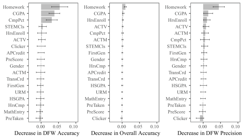
Figure 1: Variable importance of the optimized model predicting DFW for Sample 2 using institutional data and data available in-class at the end of week 2. Error bars are one standard deviation in length.

A model using only the institutional variables was first constructed to determine how well DFW students could be identified using only variables available before the semester begins. This model (Institutional) had superior performance characteristics to the Overall model of Sample 1 which used the same variables and a larger sample collected over a longer time period. The improved performance quite possibly was the result of Sample 1 averaging over many instructional environments while Sample 2 contained data from a single instructional design. This suggests that limiting the data used for the classifier to the current implementation of a course may produce superior results, even with lower sample size.

The performance of models using only the in-class data easily available to instructors consistently performed more weakly than those which mixed in-class and institutional data. The in-class-only models improved as the class progressed and became better than the model including only institutional data after the first test was given in week 5. The in-class-only model was substantially better than the institutional model after the second test was given in week 8. As such, if the goal of a classification algorithm is to predict student outcomes well into the class, only in-class data is needed.

The models combining in-class and institutional data added surprisingly little predictive power to the institutional model, particularly early in the class. This further supports the need to access a rich set of institutional data for accurate classification early in a class and suggests predictions made using only institutional data will not be substantially modified using in-class data until the first test is given.

III.1.3 Sample 3

As shown in Table 1, Sample 3 contains many fewer variables than Sample 1. The classification model for Sample 3 had lower DFW accuracy and precision than similar models for Samples 1 and 2. Restricting the variable set of Sample 1 to be approximately that of Sample 3 (the Reduced model) produced a classifier with similar properties to that of Sample 3. The difference in classification accuracy, therefore, seems to be the result of the difference in the variables available and not the difference in sample size or differences between the universities.

The student population of Sample 3 is substantially more diverse than that of Sample 1 or 2. Model performance predicting only the outcomes of minority demographic subgroups was approximately that of the overall model performance with somewhat lower variation than Sample 1. This suggests that the differences in model performance for demographic subgroups observed in Sample 1 were not a result of the low representation of those groups in the sample. Low SES students were also analyzed separately; the model performance for low SES students was similar to the overall model performance.

III.2 Variable Importance

Once constructed, classification models can provide physics instructors and departments a much more nuanced picture of student risk and provide tools to better serve their students. This section and the next section will introduce some of the additional insights which can be extracted once a classification model is constructed.

Institutional data is exceptionally complex; random forest classification models allow the identification of the parts of the institutional data that are important for the prediction of student risk and the thresholds in that data that go into classifying a student as at-risk.

The first measure useful in further understanding which variables are most important in the classification process is “variable importance.” The importance of a variable to one of the model characterization metrics such as DFW accuracy is computed by fitting the model with the variable and then without the variable to determine the mean decrease in the characterization measure when the variable is removed from the model. Figure 1 shows the mean decrease in DFW accuracy, DFW precision, and overall accuracy as the different variables used in the full model are removed for Sample 2 using data available in the second week of the class. Similar plots for Samples 1 and 3 are presented in the Supplemental Material sup .

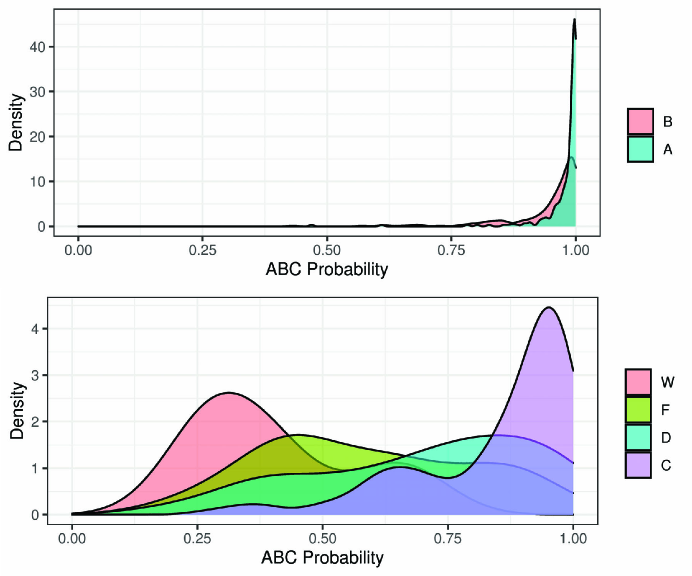
Figure 2: Predicted probability of earning an A, B, or C for Sample 1 disaggregated by the actual grade received in the class. The figure plots the probability density of each outcome. The order of the peaks in the lower figure from left to right is W, F, D, C.

The variable importance plots shown in Fig. 1 show that homework average followed by CGPA were the most important variables in accurately identifying DFW students. In addition to these variables, only CmpPct (the percentage of credit hours complete) has an error bar that does not include zero. These results are very different than the variable importance results of Study 1 which predicted the AB outcome and used overall accuracy to measure model performance. In Study 1, while homework grade grew in variable importance from week to week, it was less important than CGPA until week 5 when test 1 was given. As in Study 1, a very limited number of institutional variables were needed to predict grades in a physics class.

While many instructors would select CGPA as an important variable and would hope that homework averages were important, quantitatively having a relative measure of importance is valuable. The variable importance plots in Fig. 1 also identify many variables that seem important such as HSGPA, ACTM, and demographic variables, which were not important for the prediction of the DFW outcome.

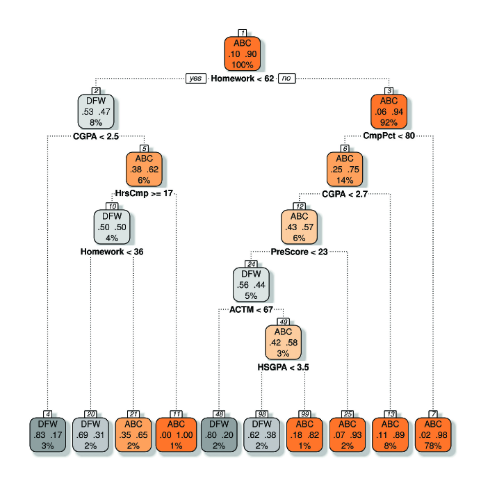
Figure 3: Decision tree for predicting the DFW outcome for Sample 2 using institutional data and data available in-class at the end of week 2.

III.3 Applying Classification Models

The most basic output of a classification model is the assignment of each student in the dataset into one of two classes: those students likely to receive and A, B, or C and those likely to receive a D, F, or W. Classification algorithms, once constructed, can provide a finer grained picture of student risk that may be more useful in applying machine learning results to manage instructional interventions for at-risk students. A classification model can also provide the probability a student will receive each outcome. The predicted probability density distribution of receiving an A, B, or C is plotted for each actual grade outcome in Fig. 2. Two plots are provided to improve readability. The distribution of probability estimates of students who actually earn an A or B is very narrow with most students with a predicted probability above 0.75. This suggests that the students who actually receive A or B in the class are predicted to receive an A, B, or C with very high probability. The probability curve for students earning a C is much broader but still peaked near one. Examination of the C distribution illustrates two key features of the prediction: (1) the vast majority of students who actually earn a C are predicted to do so with probability $p>0.5$ and (2) some students who receive a C are predicted to do so with very low probability. As such, an instructor should not interpret a low probability of receiving a C as a guarantee that a student will not succeed in the class. The probability distributions of the F and W outcomes are very broad showing these students are very difficult to predict accurately. Examination of these distributions can help instructors understand how an individual student’s probability estimate translates into actual grade outcomes and inform risk decisions.

Variable importance plots quantify the relative importance of the many variables used in the classification model correcting for the collinearity of many of the variables. These plots, however, do not provide information about the levels of these variables important in making the classification. A random forest grows thousands of decision trees on a subset of the variables; examining a single decision tree using all variables can show the thresholds for the important variables. The decision tree for the training dataset of Sample 2 in week 2 of the class is shown in Fig. 3. Each node in the tree is labeled with the majority member of the node, either ABC or DFW. The root node (top node) contains the entire training dataset, indicated by the 100% at the bottom node. Every node indicates the fraction of the training dataset contained in the node. The fraction of each outcome is shown in the center of the node; for example, the root node contains 10% DFW students and 90% ABC students. The decision condition is printed below the node. If the condition is true for the student, the left branch of the tree is taken; if false, the right branch is taken. For example, the decision condition for the root node is whether the week 2 homework average is above or below 62%. For the 8% of the students below this average, the left branch is taken to node 2. Only 47% of the students in node 2 receive an A, C, or C. For the 3% of these students with CGPA less than 2.5, only 17% receive an A, B, or C (node 4). The decision tree gives a very clear picture of the relative variable importance (higher variables in the tree are more important) and the threshold of risk of receiving a D, F, or W at each level of the tree.

IV Discussion

This study sought to answer three research questions; they will be addressed in the order proposed.

RQ1: How can machine learning algorithms be applied to predict unbalanced physics class outcomes? Study 1 used random forests and logistic regression to predict which students would receive an A or B in introductory physics. The default random forest parameters were used to build the models and the models were characterized by their overall accuracy, $\kappa$, and AUC. Because the outcome variable was fairly balanced, with 63% of the students receiving an A or B, overall accuracy provided an acceptable measure of model performance. The pure guessing accuracy was 63%, and therefore, this statistic could vary over the range 63% to 100% as variables were added to the model.

In the current work, the methods introduced in Study 1 were unproductive because the outcome variable, predicting the DFW outcome, was substantially unbalanced with only 10% (Sample 2) to 20% (Sample 3) of the students receiving this outcome. For this outcome, the pure guessing overall accuracy (simply predicting everyone receives an A, B, or C) is from 80% to 90% making it an inappropriate statistic to judge model quality. This work introduced the DFW accuracy and precision as more useful statistics to evaluate model performance. In Sample 1, using the default random forest algorithm parameters (Table 5, Default model) produced a model with very low DFW accuracy identifying only 16% of the students who actually received a D, F, or W in the test dataset; however, 57% of its predictions were correct. This does not necessarily make it a bad model, rather a model that is tuned for a specific purpose where it is much more important for the predictions to be correct than it is to identify the most potentially at-risk students. This might be useful for an application that tries to identify students for a high cost or non-negligible-risk intervention where only the most likely at-risk students could be accommodated.

Multiple methods were explored to improve model performance: oversampling, undersampling, hyperparameter tuning, and grid search. This exploration is described in the Supplemental Material sup . All methods improved the balance of DFW accuracy and precision. Oversampling led to models that overfit the data and was not used. Grid search showed that, for this dataset, it was always possible to use hyperparameter tuning by adjusting the decision threshold without having to undersample to produce a model with a balance of DFW accuracy and precision. The decision threshold for models in Table 5 excluding the default model and the models applied only to underrepresented groups was adjusted for each model to balance DFW accuracy and precision. For the overall model of Sample 1, this produced a model with substantially higher DFW accuracy and $\kappa$ that the default model; however, it still only identified 43% of the students who would receive a D, F, or W, DFW accuracy= 0.43, and had $\kappa=0.36$ in the range fair agreement by Cohen’s criteria.

Sample 2 restricted the time frame in which the institutional data were collected to a 3-year period in which the course studied had a consistent instructional environment. Even though the size of the sample was much smaller, model performance was improved showing that it is important to collect the training sample for a period where the class was presented in the same form as the class in which the model will be used.

The Sample 2 model using only institutional variables was much better than models using only in-class variables early in the semester. If an instructor wants to develop classification models for prediction of students at risk early in the semester, accessing a set of institutional data can substantially improve the models. The combination of institutional and in-class variables gave the highest model performance with an improvement of 3% in week 1, 6% in week 2, 9% in week 5 (when test 1 grades were available), and 18% in week 8 (when test 2 grades were available) compared to the model containing only institutional variables. As such, for identification of at-risk students early in the semester most of the prediction accuracy can be achieved with institutional data alone.

Sample 3 included a more restricted set of institutional variables than Sample 1, but included a variable indicating socioeconomic status and featured a more demographically diverse population. The overall model for this sample had weaker performance metrics than the overall model for Sample 1 or the institutional model for Sample 2. When the set of variables used in Sample 1 was restricted to be approximately those used in Sample 3, model performance was commensurate. It is, therefore, important for improving model performance to work with institutional research to provide the machine learning algorithms with as rich a set of data as possible.

RQ2: Does classification accuracy differ for underrepresented groups in physics? If so, how and why does it differ? For Samples 1 and 3, once the model was constructed for the full training dataset, the overall model was used to classify demographic subgroups in the test dataset separately as shown in Table 5. These models examined women, URM students, first-generation college students, and low SES students. In both samples, the model performance metrics for some minority demographic groups were different (either better or worse) than the overall model; however, these differences were within one standard deviation of the overall model. As such, the classifier built on the full training dataset predicted the outcomes of underrepresented physics students with approximately equal accuracy. While the differences observed in Table 5 are within the error of the sample, should significant differences be detected, it is possible to re-tune the models for each underrepresented group separately.

Figure 1 and similar figures in the Supplemental Material sup show the demographic variables, gender, URM, FirstGen, and SES are of low importance in the classification models. This is likely because these factors already have a general effect on other variables included in the models such as CGPA. The Supplemental Material sup includes an analysis which undersamples the majority demographic class (for example, men) to produce a more balanced dataset (for example, a dataset with the same number of men and women) (Supplemental Figs. 7 to 9). The variable importance of the demographic variables used in this study was fairly consistent with the rate of undersampling showing that the low importance was not simply a result of the lower number of students from minority demographic groups in the sample.

To further investigate the low variable importance of the demographic variables, we examined a more diverse population (Sample 3). Model performance metrics were consistent with those obtained from Sample 1, suggesting the low variable importance was not the result of the restricted number of underrepresented students in the sample.

RQ3: How can the results of a machine learning analysis be used to better understand and improve physics instruction? Once a classification model is constructed, the same model can be used to characterize new groups of students. Sections III.2 and III.3 presented three different possible analyses that can be performed with classification models that have classroom applications.

The first analysis computed the variable importance of each variable in the classifier, Fig. 1. This is done by finding the mean decrease in some performance metric if the variable is removed from the model. This analysis allows the identification of the variables which are most predictive of a student receiving a D, F, or W. This can show a working instructor where to look in complex institutional datasets and allow departments to shape their data requests.

The second analysis computed a probability of receiving an A, B, or C for each individual student. This was plotted for each actual grade received in Fig. 2. This allows an individual quantitative risk to be applied to each student. This risk could be updated as the semester progresses based on in-class performance.

The final analysis computed a decision tree, Fig. 3. This tree shows the decision thresholds which indicate the levels of the variable that are important in classifying at-risk students. As long as the instructional setting and assignment policy remains consistent, these trees can be reused semester to semester without having to rerun the analysis. The tree shows that homework average, CGPA, and the percent of hours completed were important in the decision to classify a student at risk of a DFW outcome.

These analysis results represent examples of the additional tools classification algorithms can provide instructors; many more examples could be given. The following represent some of the applications of these results being considered at Institution 1. These applications are designed around the principle that any additional instructional activity must potentially benefit all students. The models are far from perfect and, as such, all students may actually be at risk so any intervention must be available to any student.

Informing Resource Allocation: Students in physics classes at Institution 1 elect laboratory sections where a substantial part of the interactive instruction in the course is presented. Because a success probability can be generated for each student, an average probability of success could be calculated for each laboratory section. More experienced teaching assistants could be assigned to these sections. The department also has a Learning Assistant (LA) Otero et al. (2010) program using a for-credit model. Learning Assistants are not available for all lab sections; allocation of LAs to at-risk lab sections could be prioritized.

Planning Revised Assignment Policy: The decision tree in Fig. 3 and variable importance measures in Fig. 1 shows that homework grades in the second week of the class are the most important variable for predicting success and gives a homework score threshold of 62% as the highest level decision for predicting success or failure. To develop the habit of completing homework and investing sufficient effort to do well on homework, a policy allowing the reworking of homework assignments which received a grade of less than 60% for additional (or initial) credit could be implemented early in the class.

Planning Student Communication: Instructors can use the variable importance results to provide general advice to students with low homework grades and encourage them to seek additional help by attending office hours or to change habits so homework assignments are started earlier and sufficient time is allowed for completion. In general, an instructor of a large service course does not have time to personally communicate with each student; however, the combination of the individual success probability, variable importance, and variable decision threshold would allow an instructor to monitor and communicate directly with a small subset of students particularly at risk in the class. These communications could let the students know that the instructor noticed that early homework assignments needed additional work and suggest strategies to the students for improvement opening channels of personal communication with at-risk students.

Many other potential instructional uses of this type of analysis are possible. Naturally, if the intervention is successful, it will modify student outcomes changing students’ risk profiles. The classifier will need to be rebuilt using student outcomes after the implementation of the intervention to reflect this modified risk.

While using the random forest algorithm to make predictions is technically fairly straightforward for instructors trained in physics (the base code is presented in the Supplemental Material sup ), obtaining the institutional dataset may present a substantial barrier for overworked instructors of large service introductory classes. As such, we present some recommendations for managing the process of obtaining institutional data.

Gathering additional data for use by instructors should probably be the responsibility of a departmental committee or staff. The data required for different classes are quite similar. A departmental data committee would also be able to establish ethical standards for the use and handling of the data. Some effort will be needed to understand the data available at the institutional level and to work with institutional research to fine tune the data request. For example, if one requests a basic set of demographic and descriptive variables about students enrolled in a course over a number of semesters, the GPA variable provided will probably be the student’s current GPA where one actually wants the student’s GPA before he or she enrolled in the class of interest. Some interaction would also be required to develop variables such as the student’s math readiness or the fraction of classes completed. However, once a set of variables is identified, institutional records can quickly generate the data for the department each semester. Once the institutional data is acquired and understood, applying the machine learning code is fairly straightforward. It is also worth pursuing the possibility that institutional research could handle the entire process and provide a machine learning risk analysis to interested instructors. Student retention is of vital interest to most institutions with retention in core mathematics and science classes an important part of the puzzle.

V Ethical Considerations

The results of a machine learning classification represent a new tool for physics instructors to shape instruction; as with any tool, it can be correctly used or misused. If an instructor is to use the predictions of a classification algorithm, it is important that these results do not bias his or her treatment of individual students. Figure 2 shows that it is possible for students with very low predicted probability of earning an A, B, or C to get a C or higher in the class. Machine learning algorithms will never be 100% accurate and this should be taken into account in any application of the results of the algorithms. Further, while the classification results may be used to direct resources to the students most at risk, this should be done with the goal of improving instruction for all students. Machine learning results should also not be used to exclude students from additional educational activities to support at-risk students. Because the predictions are not 100% accurate, additional tutoring sessions or similar resources should be available to all; however, the results of classification models could be used to deliver encouragement to the students most at risk to avail themselves of these opportunities.

VI Conclusions

This work applied the random forest machine learning algorithm to predict whether introductory mechanics students would receive a grade of D or F, or withdraw from a physics class. Metrics and methods applied in previous work produced classification models with poor performance; however, selecting metrics appropriate for unbalanced outcomes and tuning the random forest models greatly improved the classification accuracy of the DFW outcome. Classification models performed similarly for students from two institutions with very different demographic characteristics. Models with a richer set of institutional variables were somewhat (7%) more accurate than models with a limited set of variables. The addition of in-semester variables, particularly homework averages and test scores, improved model performance. The institutional model far outperformed a model using only in-semester variables early in the semester; the performance of the in-semester only models exceeded that of the institutional only models once the first test was included as a variable. The classifier trained on the full set of students produced somewhat different performance for women, underrepresented minority students, and first-generation college students with some metrics improved and some weaker for these students. Once a classifier is constructed, multiple new analyses are available allowing the direction of additional resources to at-risk students.