High order, semi-implicit, energy stable schemes for gradient flows

Abstract

We introduce a class of high order accurate, semi-implicit Runge-Kutta schemes in the general setting of evolution equations that arise as gradient flow for a cost function, possibly with respect to an inner product that depends on the solution, and we establish their energy stability. This class includes as a special case high order, unconditionally stable schemes obtained via convexity splitting. The new schemes are demonstrated on a variety of gradient flows, including partial differential equations that are gradient flow with respect to the Wasserstein (mass transport) distance.

65M12, 65L06, 65L20

1 Introduction

We are concerned with numerical schemes for evolution equations that arise as gradient flow (steepest descent) for an energy $f:H\rightarrow\mathbb{R}$, where $H$ is a Hilbert space with inner product $\langle\cdot,\cdot\rangle$:

(1) $$u^{\prime}=-\nabla_{H}E(u).$$

Additionally, we will study gradient flows with a solution dependent inner product:

(2) $$u^{\prime}=-\mathcal{L}(u)\nabla_{H}E(u)$$

where $\mathcal{L}(u)$ is a positive definite operator that depends on $u$.

Equations Eq. 1 and Eq. 2 may represent (scalar or vectorial) ordinary or partial differential equations. One property of Eq. 1 and Eq. 2 is dissipation: $\frac{d}{dt}E(u)\leq 0$, to see this

$$\frac{d}{dt}E(u)=\langle\nabla_{H}E(u),u^{\prime}\rangle=-\langle\nabla_{H}E(u),\mathcal{L}(u)\nabla_{H}E(u)\rangle\leq 0.$$

In [12] the authors focused on unconditionally stable numerical methods to solve Eq. 1. In this paper, our focus is on semi-implicit methods that come with a rigorously established energy stability property inherited from the above expression of dissipation. Specifically let

(3) $$E(u)=E_{1}(u)+E_{2}(u)$$

where in our numerical implementation we will handle $E_{1}$ implicitly and $E_{2}$ explicitly. We allow any choice for $E_{1}$ and $E_{2}$ as long as (3) is satisfied. Our numerical methods will guarantee that when the time step is less than a constant depending only on $E_{2}$ the following numerical dissipation property will hold:

(4) $$E(u_{n+1})\leq E(u_{n})$$

where $u_{n}$ denotes the approximation to the solution at the $n$-th time step.

A basic semi-implicit scheme for the abstract equation Eq. 1, with time step size $k>0$, reads

(5) $$\frac{u_{n+1}-u_{n}}{k}=-\nabla_{H}E_{1}(u_{n+1})-\nabla_{H}E_{2}(u_{n}).$$

Let $L_{2}(u,u_{n})$ be the linearization of $E_{2}$ around $u_{n}$ so

$$L_{2}(u,u_{n})=E_{2}(u_{n})+\langle\nabla_{H}E_{2}(u_{n}),u-u_{n}\rangle$$

Then Eq. 5 is the Euler-Lagrange equation for the optimization problem

(6) $$u_{n+1}=\operatorname*{arg\,min}_{u}E_{1}(u)+L_{2}(u,u_{n})+\frac{1}{2k}\left\|u-u_{n}\right\|^{2}$$

where $\|\cdot\|^{2}=\langle\cdot,\cdot\rangle$. For

(7) $$\Lambda=\max\{0,\max_{u,\left\|v\right\|=1}D^{2}E_{2}(u)\big{(}v,v\big{)}\}$$

where by $D^{2}E_{2}(u)\big{(}v,w\big{)}$ we mean $\left.\frac{d^{2}}{d\epsilon_{2}d\epsilon_{1}}E_{2}(u+\epsilon_{1}v+\epsilon_{2}w)\right|_{\epsilon_{1}=\epsilon_{2}=0}.$ We have

(8) $$E_{2}(u)\leq L_{2}(u,p)+\frac{\Lambda}{2}\left\|u-p\right\|^{2}$$

for any $u$ and $p$. It follows that when $k\leq\frac{1}{\Lambda}$

$$E(u_{n+1}) =E_{1}(u_{n+1})+E_{2}(u_{n+1})\leq E_{1}(u_{n+1})+L_{2}(u_{n+1},u_{n})+\frac{1}{2k}\left\|u_{n+1}-u_{n}\right\|^{2}$$

$$\leq E_{1}(u_{n})+L_{2}(u_{n},u_{n})+\frac{1}{2k}\left\|u_{n}-u_{n}\right\|^{2}=E_{1}(u_{n})+E_{2}(u_{n})=E(u_{n})$$

so that scheme Eq. 5 is stable under this condition on the time step $k$, provided that optimization problem Eq. 6 can be solved.

Our new class of methods has no assumption (e.g. convexity, concavity) on the components $E_{1}$ and $E_{2}$ of the energy that are treated implicitly and explicitly, respectively. They have high (at least up to third) order accuracy. Our stability results are conditional, but revert to unconditional stability when $E_{1}$ and $E_{2}$ have appropriate convexity properties, and contain as a special case previous unconditional stability results for high order, convexity splitting type schemes. In particular, a previous paper on higher order ARK IMEX energy stable schemes [10] studies, in the spirit of convexity splitting [5], formulations that break up the energy into convex and concave parts, and treat the convex part implicitly and the concave part explicitly. We know of no other work on ARK IMEX methods that considers energy stability.

Another novelty of the present paper is extending these high order, stable, implicit and semi-implicit methods for general gradient flows to solve Eq. 2, the case when the inner product is solution dependent. There are certainly existing stable methods for Eq. 2 on a case by case basis, for example for the Cahn-Hillard equation with degenerate mobility [2, 6] and the porous medium equation [3, 4, 11]. To our knowledge, this is the first time energy stable, high order schemes for general gradient flows with solution dependent inner products have been developed.

The rest of the paper is organized as follows:

• Section 2 presents the conditions for energy stability and constructs schemes that satisfy them.

• In Section 3, we state the consistency equations for the ARK IMEX schemes for solving gradient flows Eq. 1 and give 2nd and 3rd order examples.

• Section 4 gives 2nd and 3rd order methods for solving gradient flows with solution dependent inner product Eq. 2 and provides consistency calculations.

• In Section 5, we present numerical convergence studies several of well-known partial differential equations that are gradient flows, including with respect to Wasserstein metrics.

The code for Section 5 is publicly available, and can be found at https://github.com/AZaitzeff/SIgradflow.

2 Stability of Our New Schemes

In this section, we formulate a wide class of numerical schemes that are energy stable by construction. The first of these schemes are Implicit-Explicit Additive Runge-Kutta (ARK IMEX) schemes, but we will write them in variational form in order to prove energy stability more easily. The variational formulation of our $M$-stage ARK IMEX scheme is:

1. Set $U_{0}=u_{n}$.

2. For $m=1,\ldots,M$:

   (9) $$U_{m}=\operatorname*{arg\,min}_{u}\bigg{(}E_{1}(u)+\sum^{m-1}_{i=0}\theta_{m,i}L_{2}(u,U_{i})+\sum^{m-1}_{i=0}\frac{\gamma_{m,i}}{2k}\left\|u-U_{i}\right\|^{2}\bigg{)}.$$

   where

   (10) $$L_{2}(u,p)=E_{2}(p)+\langle\nabla_{H}E_{2}(p),u-p\rangle$$

3. Set $u_{n+1}=U_{M}$.

The schemes for approximating a gradient flow with respect to a solution dependent inner product will be a series of embedded ARK IMEX methods. The inner product will be fixed for each ARK IMEX step, allowing the stability results of this section to apply. Now we establish quite broad conditions on the coefficients $\gamma_{m,i}$ $\theta_{m,i}$ that ensure conditional energy dissipation Eq. 4. Before we state and prove the conditions in generality, consider the following two-stage special case of scheme Eq. 9:

(11) $$U_{1}=\operatorname*{arg\,min}_{u}\bigg{(}E_{1}(u) +L_{2}(u,u_{n})+\frac{\gamma_{1,0}}{2k}\left\|u-u_{n}\right\|^{2}\bigg{)}$$

(12) $$\begin{split}u_{n+1}=\operatorname*{arg\,min}_{u}\bigg{(}E_{2}(u)&+\theta_{2,1}L_{2}(u,U_{1})+\theta_{2,0}L_{2}(u,u_{n})\\ &+\frac{\gamma_{2,0}}{2k}\left\|u-u_{n}\right\|^{2}+\frac{\gamma_{2,1}}{2k}\left\|u-U_{1}\right\|^{2}\bigg{)}\end{split}$$

Let $\Lambda=\max\{0,\max_{x,\left\|v\right\|=1}D^{2}E_{2}(x)\big{(}v,v\big{)}\}$. Note that this implies

(13) $$E_{2}(u)\leq L_{2}(u,p)+\frac{\Lambda}{2}\left\|u-p\right\|^{2}$$

for any $u$ and $p$. Also note that $L_{2}(u,u)=E_{2}(u)$. Impose the conditions

(14) $$\begin{split}&\gamma_{1,0}-k\Lambda-\frac{(\gamma_{2,0}-k\Lambda\theta_{2,0})^{2}}{(\gamma_{2,0}+\gamma_{2,1}-k\Lambda\theta_{2,0}-k\Lambda\theta_{2,1})}\geq 0\mbox{, }\\ &\gamma_{2,1}+\gamma_{2,0}-k\Lambda\theta_{2,0}-k\Lambda\theta_{2,1}>0\mbox{, }\\ &\theta_{2,1}+\theta_{2,0}=1\mbox{ and }\\ &\theta_{2,1},\theta_{2,0}\geq 0\end{split}$$

on the parameters. Set $\mu=\frac{\gamma_{2,0}-k\Lambda\theta_{2,0}}{\gamma_{2,0}+\gamma_{2,1}-k\Lambda\theta_{2,0}-k\Lambda\theta_{2,1}}$. First note that (12) is equivalent to

(15) $$u_{n+1}=\operatorname*{arg\,min}_{u}E_{1}(u)+\theta_{2,1}L_{2}(u,U_{1})+\theta_{2,0}L_{2}(u,u_{n})+\theta_{2,0}\Lambda\left\|u-u_{n}\right\|^{2}+\\ \theta_{2,1}\Lambda\left\|u-U_{1}\right\|^{2}+\frac{\gamma_{2,0}+\gamma_{2,1}-k\Lambda\theta_{2,0}-k\Lambda\theta_{2,1}}{2k}\left\|u-\big{(}\mu u_{n}+(1-\mu)U_{1}\big{)}\right\|^{2}.$$

This can be seen by expanding the norm squared and comparing the quadratic and linear terms in $u$. With these tools in hand we can prove energy dissipation:

$$E(u_{n+1})$$

$$= E_{1}(u_{n+1})+E_{2}(u_{n+1})$$

$$\leq E_{1}(u_{n+1})+\theta_{2,1}[L_{2}(u_{n+1},U_{1})+\frac{\Lambda}{2}\left\|u_{n+1}-U_{1}\right\|^{2}]$$

$$+\theta_{2,0}[L_{2}(u_{n+1},u_{n})+\frac{\Lambda}{2}\left\|u_{n+1}-u_{n}\right\|^{2}]$$ (by (13))

$$\leq E_{1}(u_{n+1})+\theta_{2,1}[L_{2}(u_{n+1},U_{1})+\frac{\Lambda}{2}\left\|u_{n+1}-U_{1}\right\|^{2}]$$

$$+\theta_{2,0}[L_{2}(u_{n+1},u_{n})+\frac{\Lambda}{2}\|u_{n+1}-u_{n}\|^{2}]$$

$$+\frac{\gamma_{2,0}+\gamma_{2,1}-k\Lambda\theta_{2,0}-k\Lambda\theta_{2,1}}{2k}\left\|u_{n+1}-\big{(}\mu u_{n}+(1-\mu)U_{1}\big{)}\right\|^{2}.$$ (by (14))

$$\leq E_{1}(U_{1})+\theta_{2,1}E_{2}(U_{1})+\theta_{2,0}[L_{2}(U_{1},u_{n})+\frac{\Lambda}{2}\|U_{1}-u_{n}\|^{2}]$$

$$+\frac{\gamma_{2,0}+\gamma_{2,1}-\Lambda\theta_{2,0}-\Lambda\theta_{2,1}}{2k}\left\|U_{1}-\big{(}\mu u_{n}+(1-\mu)U_{1}\big{)}\right\|^{2}$$ (by (15))

$$\leq E_{1}(U_{1})+\theta_{2,1}[L_{2}(U_{1},u_{n})+\frac{\Lambda}{2}\|u_{n+1}-u_{n}\|^{2}]$$

$$+\theta_{2,0}[L_{2}(U_{1},u_{n})+\frac{\Lambda}{2}\|U_{1}-u_{n}\|^{2}]$$

$$+\frac{(\gamma_{2,0}-k\theta_{2,0})^{2}}{(\gamma_{2,0}+\gamma_{2,1}-k\Lambda\theta_{2,0}-k\Lambda\theta_{2,1})2k}\left\|U_{1}-u_{n}\right\|^{2}$$

$$\leq E_{1}(U_{1})+[L_{2}(U_{1},u_{n})+\frac{\Lambda}{2}\|U_{1}-u_{n}\|^{2}]+\frac{\gamma_{1,0}-k\Lambda}{2k}\left\|U_{1}-u_{n}\right\|^{2}$$ (by (13))

$$\leq E(u_{n}).$$ (by (11))

The first two conditions of Eq. 14 require $k$ to be below a certain threshold. Hence the dissipation of Eq. 11 & Eq. 12 is conditional, unless $E_{2}$ happens to be concave, in which case these two conditions are satisfied for all $k>0$.

We will now extend this discussion to general, $M$-stage case of scheme Eq. 9:

Theorem 2.1.

Fix a time step $k$. Define $\Lambda=\max\{0,\max_{x,\left\|v\right\|=1}D^{2}E_{2}(x)\big{(}v,v\big{)}\}$ and the following auxiliary quantities in terms of the coefficients $\gamma_{m,i}$ and $\theta_{m,i}$ of scheme Eq. 9:

(16) $$\tilde{\gamma}_{m,i}=\gamma_{m,i}-k\Lambda\theta_{m,i}-\sum_{j=m+1}^{M}\tilde{\gamma}_{j,i}\frac{\tilde{S}_{j,m}}{\tilde{S}_{j,j}}$$

(17) $$\tilde{S}_{j,m}=\sum_{i=0}^{m-1}\tilde{\gamma}_{j,i}$$

If $\tilde{S}_{m,m}>0$ for $m=1,\ldots,M$, $\theta_{m-1,i}\geq\theta_{m,i}\geq 0$ and $\sum_{i=0}^{m-1}\theta_{m,i}=1$, then scheme Eq. 9 satisfies the energy stability condition Eq. 4: For every $n=0,1,2,\ldots$ we have $E(u_{n+1})\leq E(u_{n})$.

As we will see in Section 3, the conditions on the parameters $\gamma_{i,j}$ and $\theta_{m,i}$ of scheme Eq. 9 imposed in Theorem 2.1 are loose enough to enable meeting consistency conditions to high order. We will establish Theorem 2.1 with the help of a couple of lemmas:

Lemma 2.2.

Let the auxiliary quantities $\tilde{S}_{j,m}$, and $\tilde{\gamma}_{m,i}$ be defined as in Theorem 2.1. We have

$$\operatorname*{arg\,min}E(u)+\sum^{m-1}_{i=0}\theta_{m,i}L_{2}(u,U_{i})+\sum^{m-1}_{i=0}\frac{\gamma_{m,i}}{2k}\left\|u-U_{i}\right\|^{2}$$

$$= \operatorname*{arg\,min}E(u)+\sum^{m-1}_{i=0}\theta_{m,i}[L_{2}(u,U_{i})+\frac{\Lambda}{2}\left\|u-U_{i}\right\|^{2}]+\frac{1}{2k}\sum_{j=m}^{M}\frac{\tilde{S}_{j,m}^{2}}{\tilde{S}_{j,j}}\left\|u-\sum_{i=0}^{m-1}\frac{\tilde{\gamma}_{j,i}}{\tilde{S}_{j,m}}U_{i}\right\|^{2}$$

Proof 2.3.

As in the two step case the proof consists of expanding the norm squared terms and showing that all the quadratic and linear terms of $u$ are equal. First, the expansion of $\sum^{m-1}_{i=0}\frac{\gamma_{m,i}}{2k}\|u-U_{i}\|^{2}$ is

(18) $$\frac{\|u\|^{2}}{2k}\sum^{m-1}_{i=0}\gamma_{m,i}-\frac{1}{k}\langle u,\sum^{m-1}_{i=0}\gamma_{m,i}U_{i}\rangle+\text{terms that do not depend on $u$.}$$

Next, we will establish two identities to help us expand

$$\frac{1}{2k}\sum_{j=m}^{M}\frac{\tilde{S}_{j,m}^{2}}{\tilde{S}_{j,j}}\|u-\sum_{i=0}^{m-1}\frac{\tilde{\gamma}_{j,i}}{\tilde{S}_{j,m}}U_{i}\|^{2}.$$

First by rearranging Eq. 16,

(19) $$\gamma_{m,i}-k\Lambda\theta_{m,i}=\sum_{j=m}^{M}\tilde{\gamma}_{j,i}\frac{\tilde{S}_{j,m}}{\tilde{S}_{j,j}}.$$

Next, an identity of $\tilde{S}_{m,m}$:

$$\tilde{S}_{m,m} =\sum_{i=0}^{m-1}\tilde{\gamma}_{m,i}=\sum_{i=0}^{m-1}\bigg{[}\gamma_{m,i}-k\Lambda\theta_{m,i}-\sum_{j=m+1}^{M}\tilde{\gamma}_{j,i}\frac{\tilde{S}_{j,m}}{\tilde{S}_{j,j}}\bigg{]}$$

$$=\sum_{i=0}^{m-1}\bigg{[}\gamma_{m,i}-k\Lambda\theta_{m,i}\bigg{]}-\sum_{j=m+1}^{M}\bigg{[}\sum_{i=0}^{m-1}\tilde{\gamma}_{j,i}\bigg{]}\frac{\tilde{S}_{j,m}}{\tilde{S}_{j,j}}$$

$$=\sum_{i=0}^{m-1}\bigg{[}\gamma_{m,i}-k\Lambda\theta_{m,i}\bigg{]}-\sum_{j=m+1}^{M}\frac{\tilde{S}_{j,m}^{2}}{\tilde{S}_{j,j}}.$$

We use this identity to establish the following:

(20) $$\sum_{j=m}^{M}\frac{\tilde{S}_{j,m}^{2}}{\tilde{S}_{j,j}}=\tilde{S}_{m,m}+\sum_{j=m+1}^{M}\frac{\tilde{S}_{j,m}^{2}}{\tilde{S}_{j,j}}=\sum_{i=0}^{m-1}\bigg{[}\gamma_{m,i}-k\Lambda\theta_{m,i}\bigg{]}$$

Now we can calculate the expansion:

$$\frac{1}{2k}\sum_{j=m}^{M}\frac{\tilde{S}_{j,m}^{2}}{\tilde{S}_{j,j}}\|u-\sum_{i=0}^{m-1}\frac{\tilde{\gamma}_{j,i}}{\tilde{S}_{j,m}}U_{i}\|^{2}+\sum^{m-1}_{i=0}\theta_{m,i}\Lambda\left\|u-U_{i}\right\|^{2}$$

$$= \frac{\|u\|^{2}}{2k}\sum_{j=m}^{M}\frac{\tilde{S}_{j,m}^{2}}{\tilde{S}_{j,j}}-\frac{1}{k}\langle u,\sum_{i=0}^{m-1}\sum_{j=m}^{M}\tilde{\gamma}_{j,i}\frac{\tilde{S}_{j,m}}{\tilde{S}_{j,j}}U_{i}\rangle+\frac{\Lambda}{2}\|u\|^{2}\sum^{m-1}_{i=0}\theta_{m,i}+\Lambda\sum^{m-1}_{i=0}\langle u,\theta_{m,i}U_{i}\rangle$$

$$+\text{terms that do not depend on $u$}$$

$$= \frac{\|u\|^{2}}{2k}\sum^{m-1}_{i=0}\gamma_{m,i}-\frac{1}{k}\langle u,\sum^{m-1}_{i=0}\gamma_{m,i}U_{i}\rangle+\text{terms that do not depend on $u$.}$$

Where the last equality follows from Eq. 19 and Eq. 20. Since this expansion matches Eq. 18 up to a constant in $u$ the proof is complete.

Lemma 2.4.

Let $\Lambda$ and the auxiliary quantities $\tilde{S}_{j,m}$, $\tilde{\gamma}_{m,i}$ be given in Theorem 2.1. Additionally, let $\tilde{S}_{m,m}>0$ for $m=1,\ldots,M$. Then

$$E_{1}(U_{m})+\sum^{m-1}_{i=0}\theta_{m,i}[L_{2}(U_{m},U_{i})+\frac{\Lambda}{2}\left\|U_{m}-U_{i}\right\|^{2}]+\frac{1}{2k}\sum_{j=m}^{M}\frac{\tilde{S}_{j,m}^{2}}{\tilde{S}_{j,j}}\left\|U_{m}-\sum_{i=0}^{m-1}\frac{\tilde{\gamma}_{j,i}}{\tilde{S}_{j,m}}U_{i}\right\|^{2}$$

$$\leq E_{1}(U_{m-1})+\sum^{m-2}_{i=0}\theta_{m-1,i}[L_{2}(U_{m-1},U_{i})+\frac{\Lambda}{2}\left\|U_{m-1}-U_{i}\right\|^{2}]$$

$$+\frac{1}{2k}\sum_{j=m-1}^{M}\frac{\tilde{S}_{j,m-1}^{2}}{\tilde{S}_{j,j}}\left\|U_{m-1}-\sum_{i=0}^{m-2}\frac{\tilde{\gamma}_{j,i}}{\tilde{S}_{j,m-1}}U_{i}\right\|^{2}$$

Proof 2.5.

By Eq. 9 & Lemma 2.2,

$$U_{m}=\operatorname*{arg\,min}_{u}E(u)+\sum^{m-1}_{i=0}\theta_{m,i}[L_{2}(u,U_{i})+\Lambda\left\|u-U_{i}\right\|^{2}]+\frac{1}{2k}\sum_{j=m}^{M}\frac{\tilde{S}_{j,m}^{2}}{\tilde{S}_{j,j}}\|u-\sum_{i=0}^{m-1}\frac{\tilde{\gamma}_{j,i}}{\tilde{S}_{j,m}}U_{i}\|^{2}.$$

Since $U_{m}$ is the minimizer of the above optimization problem

$$E_{1}(U_{m})+\sum^{m-1}_{i=0}\theta_{m,i}[L_{2}(U_{m},U_{i})+\frac{\Lambda}{2}\left\|U_{m}-U_{i}\right\|^{2}]$$

$$+\frac{1}{2k}\sum_{j=m}^{M}\frac{\tilde{S}_{j,m}^{2}}{\tilde{S}_{j,j}}\left\|U_{m}-\sum_{i=0}^{m-1}\frac{\tilde{\gamma}_{j,i}}{\tilde{S}_{j,m}}U_{i}\right\|^{2}$$

(21) $$\begin{split}\leq&E_{1}(U_{m-1})+\theta_{m,m-1}E_{2}(U_{m-1})+\sum^{m-2}_{i=0}\theta_{m,i}[L_{2}(U_{m-1},U_{i})+\frac{\Lambda}{2}\left\|U_{m-1}-U_{i}\right\|^{2}]\\ &+\frac{1}{2k}\sum_{j=m}^{M}\frac{\tilde{S}_{j,m}^{2}}{\tilde{S}_{j,j}}\left\|U_{m-1}-\sum_{i=0}^{m-1}\frac{\tilde{\gamma}_{j,i}}{\tilde{S}_{j,m}}U_{i}\right\|^{2}\end{split}$$

We give two inequalities to aid us in the proof. First, using the definition of the auxiliary variables, we can state an identity that will simplify Eq. 21. For $m>1$ and $j\geq m$

(22) $$\begin{split}&\frac{\tilde{S}_{j,m}^{2}}{\tilde{S}_{j,j}}\left\|U_{m-1}-\sum_{i=0}^{m-1}\frac{\tilde{\gamma}_{j,i}}{\tilde{S}_{j,m}}U_{i}\right\|^{2}=\frac{\tilde{S}_{j,m}^{2}}{\tilde{S}_{j,j}}\left\|U_{m-1}\bigg{(}1-\frac{\tilde{\gamma}_{j,m-1}}{\tilde{S}_{j,m}}\bigg{)}-\sum_{i=0}^{m-2}\frac{\tilde{\gamma}_{j,i}}{\tilde{S}_{j,m}}U_{i}\right\|^{2}\\ =&\frac{\tilde{S}_{j,m}^{2}}{\tilde{S}_{j,j}}\left\|U_{m-1}\bigg{(}\frac{\tilde{S}_{j,m-1}}{\tilde{S}_{j,m}}\bigg{)}-\sum_{i=0}^{m-2}\frac{\tilde{\gamma}_{j,i}}{\tilde{S}_{j,m}}U_{i}\right\|^{2}=\frac{\tilde{S}_{j,m-1}^{2}}{\tilde{S}_{j,j}}\left\|U_{m-1}-\sum_{i=0}^{m-2}\frac{\tilde{\gamma}_{j,i}}{\tilde{S}_{j,m-1}}U_{i}\right\|^{2}.\end{split}$$

Now since $\tilde{S}_{m-1,m-1}>0$,

(23) $$\frac{\tilde{S}_{m-1,m-1}^{2}}{\tilde{S}_{m-1,m-1}}\left\|U_{m-1}-\sum_{i=0}^{m-2}\frac{\tilde{\gamma}_{m-1,i}}{\tilde{S}_{m-1,m-1}}U_{i}\right\|^{2}>0.$$

Using Eq. 22 and Eq. 23 we have

(24) $$\frac{1}{2k}\sum_{j=m}^{M}\frac{\tilde{S}_{j,m}^{2}}{\tilde{S}_{j,j}}\left\|U_{m-1}-\sum_{i=0}^{m-1}\frac{\tilde{\gamma}_{j,i}}{\tilde{S}_{j,m}}U_{i}\right\|^{2}=\frac{1}{2k}\sum_{j=m}^{M}\frac{\tilde{S}_{j,m-1}^{2}}{\tilde{S}_{j,j}}\left\|U_{m-1}-\sum_{i=0}^{m-2}\frac{\tilde{\gamma}_{j,i}}{\tilde{S}_{j,m-1}}U_{i}\right\|^{2}\\ \leq\frac{1}{2k}\sum_{j=m-1}^{M}\frac{\tilde{S}_{j,m-1}^{2}}{\tilde{S}_{j,j}}\left\|U_{m-1}-\sum_{i=0}^{m-2}\frac{\tilde{\gamma}_{j,i}}{\tilde{S}_{j,m-1}}U_{i}\right\|^{2}.$$

Next, since $\sum_{i=1}^{m-1}\theta_{m,i}=1$ for all $m$ we have the equality

(25) $$\theta_{m,m-1}=1-\sum^{m-2}_{i=0}\theta_{m,i}=\sum^{m-2}_{i=0}\theta_{m-1,i}-\sum^{m-2}_{i=0}\theta_{m,i}$$

Using Eq. 13 and Eq. 25, we have our second inequality:

(26) $$\begin{split}&\theta_{m,m-1}E_{2}(U_{m-1})+\sum^{m-2}_{i=0}\theta_{m,i}[L_{2}(U_{m-1},U_{i})+\frac{\Lambda}{2}\left\|U_{m-1}-U_{i}\right\|^{2}]\\ =&\sum^{m-2}_{i=0}(\theta_{m-1,i}-\theta_{m,i})E_{2}(U_{m-1})+\sum^{m-2}_{i=0}\theta_{m,i}[L_{2}(U_{m-1},U_{i})+\frac{\Lambda}{2}\left\|U_{m-1}-U_{i}\right\|^{2}]\\ \leq&\sum^{m-2}_{i=0}(\theta_{m-1,i}-\theta_{m,i})[L_{2}(U_{m-1},U_{i})+\frac{\Lambda}{2}\left\|U_{m-1}-U_{i}\right\|^{2}]\\ &+\sum^{m-2}_{i=0}\theta_{m,i}[L_{2}(U_{m-1},U_{i})+\frac{\Lambda}{2}\left\|U_{m-1}-U_{i}\right\|^{2}]\\ =&\sum^{m-2}_{i=0}\theta_{m-1,i}[L_{2}(U_{m-1},U_{i})+\frac{\Lambda}{2}\left\|U_{m-1}-U_{i}\right\|^{2}]\end{split}$$

Using inequalities Eq. 24 and Eq. 26, we have that Eq. 21 is less than or equal to

$$E_{1}(U_{m-1})+\sum^{m-2}_{i=0}\theta_{m-1,i}[L_{2}(U_{m-1},U_{i})+\frac{\Lambda}{2}\left\|U_{m-1}-U_{i}\right\|^{2}]\\ +\frac{1}{2k}\sum_{j=m-1}^{M}\frac{\tilde{S}_{j,m-1}^{2}}{\tilde{S}_{j,j}}\left\|U_{m-1}-\sum_{i=0}^{m-2}\frac{\tilde{\gamma}_{j,i}}{\tilde{S}_{j,m-1}}U_{i}\right\|^{2}$$

concluding the proof.

Proof 2.6.

(of theorem) The main idea of the proof is to use Lemma 2.4 repeatedly to relate the energy of $E(u_{n+1})$ to $E(u_{n})$. First, by Eq. 13 and our assumption that $\tilde{S}_{M,M}>0$

$$E(u_{n+1}) =E_{1}(U_{M})+E_{2}(U_{M})$$

$$\leq E_{1}(U_{M})+\sum^{M-1}_{i=0}\theta_{M,i}[L_{2}(U_{M},U_{i})+\frac{\Lambda}{2}\left\|U_{M}-U_{i}\right\|^{2}]$$

$$+\frac{1}{2k}\frac{\tilde{S}_{M,M}^{2}}{\tilde{S}_{M,M}}\|U_{M}-\sum_{i=0}^{M-1}\frac{\tilde{\gamma}_{M,i}}{\tilde{S}_{M,M}}U_{i}\|^{2}.$$

By using the Lemma 2.4 repeatedly we have

$$E_{1}(U_{M})+\sum^{M-1}_{i=0}\theta_{M,i}[L_{2}(U_{M},U_{i})+\frac{\Lambda}{2}\left\|U_{M}-U_{i}\right\|^{2}]+\frac{1}{2k}\frac{\tilde{S}_{M,M}^{2}}{\tilde{S}_{M,M}}\|U_{M}-\sum_{i=0}^{M-1}\frac{\tilde{\gamma}_{M,i}}{\tilde{S}_{M,M}}U_{i}\|^{2}$$

$$\leq E_{1}(U_{M-1})+\sum^{M-2}_{i=0}\theta_{M-1,i}[L_{2}(U_{M-1},U_{i})+\frac{\Lambda}{2}\left\|U_{M-1}-U_{i}\right\|^{2}]$$

$$+\frac{1}{2k}\sum_{j=M-1}^{M}\frac{\tilde{S}_{j,M-1}^{2}}{\tilde{S}_{j,j}}\left\|U_{M-1}-\sum_{i=0}^{M-2}\frac{\tilde{\gamma}_{j,i}}{\tilde{S}_{j,M-1}}U_{i}\right\|^{2}$$

$$\vdots$$

$$\leq E_{1}(U_{1})+L_{2}(U_{1},U_{0})+\frac{\Lambda}{2}\left\|U_{1}-U_{0}\right\|^{2}+\frac{1}{2k}\sum_{j=1}^{M}\frac{\tilde{S}_{j,1}^{2}}{\tilde{S}_{j,j}}\|U_{1}-\frac{\tilde{\gamma}_{j,0}}{\tilde{S}_{j,1}}U_{0}\|^{2}.$$

By Eq. 9 and Lemma 2.2

$$U_{1}=\operatorname*{arg\,min}_{u}E_{1}(u)+L_{2}(u,U_{0})+\frac{\Lambda}{2}\left\|u-U_{0}\right\|^{2}+\frac{1}{2k}\sum_{j=1}^{M}\frac{\tilde{S}_{j,1}^{2}}{\tilde{S}_{j,j}}\|u-\frac{\tilde{\gamma}_{j,0}}{\tilde{S}_{j,1}}U_{0}\|^{2}$$

so

$$E_{1}(U_{1})+L_{2}(U_{1},U_{0})+\frac{\Lambda}{2}\left\|U_{1}-U_{0}\right\|^{2}+\frac{1}{2k}\sum_{j=1}^{M}\frac{\tilde{S}_{j,1}^{2}}{\tilde{S}_{j,j}}\|U_{1}-\frac{\tilde{\gamma}_{j,0}}{\tilde{S}_{j,1}}U_{0}\|^{2}$$

$$\leq E_{1}(U_{0})+E_{2}(U_{0})+\frac{\Lambda}{2}\left\|U_{0}-U_{0}\right\|^{2}+\frac{1}{2k}\sum_{j=1}^{M}\frac{\tilde{S}_{j,1}^{2}}{\tilde{S}_{j,j}}\|U_{0}-U_{0}\|^{2}$$

$$= E(u_{n})$$

completing the proof of the theorem.

Remark 2.7.

In the above proof, we assume that $E_{2}(u)$ is two times differentiable. This assumption can be dropped if we replace $L_{2}(u,p)$ with another approximation $A_{2}(u,p)$ that has the properties $A_{2}(u,u)=E_{2}(u)$ and for some choice $\Lambda$, $E_{2}(u)\leq A_{2}(u,p)+\frac{\Lambda}{2}\left\|u-p\right\|^{2}$ for all $u$ and $p$.

3 Examples of the New Schemes for Gradient Flows

In this section, we give examples of high order semi-implicit schemes for gradient flows, for any desired choice of implicit and explicit terms $E_{1}$ and $E_{2}$, that are energy stable under the conditions of Theorem 2.1. First, we give the conditions on $\gamma_{m,i}$ and $\theta_{m,i}$ in scheme Eq. 9 to ensure high order consistency with the abstract evolution law Eq. 1. Recall that $U_{0}=u_{n}$. From Eq. 9, each stage $U_{m}$ satisfies the Euler-Lagrange equation:

(27) $$\bigg{[}\sum^{m-1}_{i=0}\gamma_{m,i}\bigg{]}U_{m}+k\nabla_{H}E_{1}(U_{m})=-\sum^{m-1}_{i=0}k\theta_{m,i}\nabla_{H}E_{2}(U_{i})+\sum^{m-1}_{i=0}\gamma_{m,i}U_{i}.$$

Eq. 27 is equivalent to the form more often seen for ARK IMEX methods:

(28) $$U_{m}=U_{0}-k\sum^{m}_{i=1}\alpha_{m,i}\nabla_{H}E_{1}(U_{i})-k\sum^{m-1}_{i=1}\tilde{\alpha}_{m,i}\nabla_{H}E_{2}(U_{i})$$

where $\alpha_{m,i}$ and $\tilde{\alpha}_{m,i}$ depend on $\gamma_{m_{i}}$ and $\theta_{m,i}$. The consistency equations for ARK IMEX methods have been previously worked out [8, 9, 10, 13]. As such, we will state without proof the conditions required to achieve various orders of accuracy in terms of $\gamma$ and $\theta$:

Claim 1.

Let $U_{i}$ be given in Eq. 9. The Taylor expansion of $U_{i}$ at each stage has the form:

(29) $$\begin{split}U_{i}&=U_{0}-\beta_{1,i}kDE(U_{0})+k^{2}\big{[}\beta_{2,i}k^{2}D^{2}E_{1}(U_{0})DE(U_{0})+\beta_{3,i}D^{2}E_{2}(U_{0})DE(U_{0})\big{]}\\ &-k^{3}\big{[}\beta_{4,i}D^{2}E_{1}(U_{0})\left(D^{2}E_{1}(U_{0})\left(DE(U_{0})\right)\right)+\beta_{5,i}D^{2}E_{1}(U_{0})\left(D^{2}E_{2}(U_{0})\left(DE(U_{0})\right)\right)\\ &+\beta_{6,i}D^{2}E_{2}(U_{0})\left(D^{2}E_{1}(U_{0})\left(DE(U_{0})\right)\right)+\beta_{7,i}D^{2}E_{2}(U_{0})\left(D^{2}E_{2}(U_{0})\left(DE(U_{0})\right)\right)\\ &+\beta_{8,i}D^{3}E_{1}(U_{0})\big{(}DE(U_{0}),DE(U_{0})\big{)}+\beta_{9,i}D^{3}E_{2}(U_{0})\big{(}DE(U_{0}),DE(U_{0})\big{)}\big{]}+\text{h.o.t.}\end{split}$$

where for $l\in\{1,2,3,\ldots\}$, $D^{l}E(u):H^{l}\to\mathbb{R}$ denotes the multilinear form given by

$$D^{l}E(u)\big{(}v_{1},\ldots,v_{n}\big{)}=\left.\frac{\partial^{l}}{\partial s_{1}\cdots\partial s_{l}}E(u+s_{1}v_{1}+s_{2}v_{2}+\cdots+s_{l}v_{l})\right|_{s_{1}=s_{2}=\cdots=s_{l}=0}$$

so that the linear functional $D^{l}E(u)\big{(}v_{1},v_{2},\ldots,v_{l-1},\cdot\big{)}:H\to\mathbb{R}$ may be identified with an element of $H$, and so on. The coefficients of Eq. 29 obey the following recursive relations:

(30) $$\begin{split}&\beta_{1,0}=\beta_{2,0}=\ldots=\beta_{9,0}=0\\ &\beta_{1,m}=\frac{1}{S_{m}}\bigg{[}1+\sum^{m-1}_{i=1}\gamma_{m,i}\beta_{1,i}\bigg{]}\\ &\beta_{2,m}=\frac{1}{S_{m}}\bigg{[}\beta_{1,m}+\sum^{m-1}_{i=1}\gamma_{m,i}\beta_{2,i}\bigg{]}\\ &\beta_{3,m}=\frac{1}{S_{m}}\bigg{[}\sum_{i=0}^{m-1}\theta_{m,i}\beta_{1,i}+\sum^{m-1}_{i=1}\gamma_{m,i}\beta_{3,i}\bigg{]}\\ &\beta_{4,m}=\frac{1}{S_{m}}\bigg{[}\beta_{2,m}+\sum^{m-1}_{i=1}\gamma_{m,i}\beta_{4,i}\bigg{]}\\ &\beta_{5,m}=\frac{1}{S_{m}}\bigg{[}\beta_{3,m}+\sum^{m-1}_{i=1}\gamma_{m,i}\beta_{5,i}\bigg{]}\\ &\beta_{6,m}=\frac{1}{S_{m}}\bigg{[}\sum_{i=0}^{m-1}\theta_{m,i}\beta_{2,i}+\sum^{m-1}_{i=1}\gamma_{m,i}\beta_{6,i}\bigg{]}\\ &\beta_{7,m}=\frac{1}{S_{m}}\bigg{[}\sum_{i=0}^{m-1}\theta_{m,i}\beta_{3,i}+\sum^{m-1}_{i=1}\gamma_{m,i}\beta_{7,i}\bigg{]}\\ &\beta_{8,m}=\frac{1}{S_{m}}\bigg{[}\frac{\beta_{1,m}^{2}}{2}+\sum^{m-1}_{i=1}\gamma_{m,i}\beta_{8,i}\bigg{]}\\ &\beta_{9,m}=\frac{1}{S_{m}}\bigg{[}\frac{1}{2}\sum_{i=0}^{m-1}\theta_{m,i}\beta_{1,i}^{2}+\sum^{m-1}_{i=1}\gamma_{m,i}\beta_{9,i}\bigg{]}\end{split}$$

with $S_{m}=\sum^{m-1}_{i=0}\gamma_{m,i}$. Furthermore, the following conditions for $u_{n+1}=U_{M}$ in scheme Eq. 9 are necessary and sufficient for various orders of accuracy:

First Order: Second Order: Third Order:

$$\beta_{1,M}=1 \beta_{1,M}=1 \beta_{1,M}=1$$

(31) $$\beta_{2,M}=1/2 \beta_{2,M}=1/2$$

$$\beta_{3,M}=1/2 \beta_{3,M}=1/2$$

$$\beta_{4,M}=\beta_{5,M}=\ldots=\beta_{9,M}=1/6$$

Now, we give second order and a third order example of method Eq. 9. However, The examples we give are not unique by any means. We begin with a five step method that is second order accurate:

(32) $$\begin{split}&\theta\approx\left(\begin{array}[]{ccccc}1.&0&0&0&0\\ 0.009&0.991&0&0&0\\ 0.009&0.991&0&0&0\\ 0&0&0&1.&0\\ 0&0&0&1.&0\\ \end{array}\right)\\ &\gamma\approx\left(\begin{array}[]{ccccc}8.841&0&0&0&0\\ -0.925&5.360&0&0&0\\ -4.443&6.041&0.950&0&0\\ -3.288&5.895&-0.351&0.172&0\\ -3.895&-0.335&4.964&-1.722&7.684\end{array}\right)\end{split}$$

which is stable for $k\Lambda\leq 3/872$.

Next we have a thirteen step method that is third order accurate:

(33) $$\begin{split}&\theta\approx\left(\begin{array}[]{ccccccccccccc}1.&0&0&0&0&0&0&0&0&0&0&0&0\\ 0.049&0.951&0&0&0&0&0&0&0&0&0&0&0\\ 0.024&0.075&0.901&0&0&0&0&0&0&0&0&0&0\\ 0.017&0.042&0.113&0.829&0&0&0&0&0&0&0&0&0\\ 0.012&0.029&0.071&0.386&0.501&0&0&0&0&0&0&0&0\\ 0.01&0.023&0.06&0.366&0.457&0.085&0&0&0&0&0&0&0\\ 0.007&0.018&0.05&0.351&0.437&0.06&0.076&0&0&0&0&0&0\\ 0.003&0.005&0.006&0.008&0.009&0.011&0.028&0.929&0&0&0&0&0\\ 0.002&0.002&0.002&0.002&0.003&0.004&0.009&0.029&0.948&0&0&0&0\\ 0&0.001&0.001&0.001&0.001&0.002&0.004&0.007&0.011&0.971&0&0&0\\ 0&0&0.001&0.001&0.001&0.001&0.003&0.005&0.008&0.912&0.069&0&0\\ 0&0&0&0&0&0.001&0.002&0.003&0.005&0.107&0.025&0.857&0\\ 0&0&0&0&0&0&0.001&0.001&0.002&0.013&0.007&0.018&0.958\\ \end{array}\right)\\ &\gamma\approx\left(\begin{array}[]{ccccccccccccc}11.&0&0&0&0&0&0&0&0&0&0&0&0\\ 2.1&15.5&0&0&0&0&0&0&0&0&0&0&0\\ 1.4&1.6&17.&0&0&0&0&0&0&0&0&0&0\\ 0.2&1.6&-2.4&18.1&0&0&0&0&0&0&0&0&0\\ 0.3&-8.5&3.&9.6&7.8&0&0&0&0&0&0&0&0\\ -1.4&-5.9&-0.1&2.&8.&4.1&0&0&0&0&0&0&0\\ -4.&-0.5&-0.4&-1.8&5.1&6.8&0.9&0&0&0&0&0&0\\ -9.2&4.8&2.7&-3.2&2.5&6.2&2.5&4.6&0&0&0&0&0\\ -1.7&-3.6&-0.1&1.3&5.7&3.4&-0.8&-0.8&0.4&0&0&0&0\\ -2.7&-3.5&0.6&1.4&6.1&3.5&-0.7&-0.2&-0.4&0.5&0&0&0\\ 5.9&-4.8&-5.1&-3.1&3.4&6.6&-0.7&-5.2&4.9&-0.8&8.2&0&0\\ 7.1&0.9&-3.1&-2.7&-5.8&-1.9&0.6&-3.4&4.3&-1.3&9.2&9.1&0\\ 3.8&1.9&2.7&2.1&-7.5&-10.6&-1.2&2.&0.7&-0.2&-0.2&9.5&12.8\\ \end{array}\right)\end{split}$$

and is stable if $k\Lambda\leq 18/28567$. The coefficients to machine precision as well as code to verify Theorem 2.1 and Claim 1 can be found at https://github.com/AZaitzeff/SIgradflow. In the following section, we consider methods for Eq. 2, when the inner product changes with the solution.

4 Schemes for Solving Gradient Flows with Solution Dependent Inner Product

Now we move on to the problem of simulating flow Eq. 2,

$$u^{\prime}=-\mathcal{L}(u)\nabla_{H}E(u).$$

We consider the case where $\mathcal{L}(u)$ is strictly positive definite. Our approach will be as follows:

1. Generate a $u_{*}$ from $u_{n}$.

2. Construct $\mathcal{L}(u_{*})$.

3. Use the algorithm Eq. 9 with norm $\left\|\cdot\right\|^{2}_{\mathcal{L}^{-1}(u_{*})}=\langle\cdot,\mathcal{L}^{-1}(u_{*})\cdot\rangle$ to generate $u_{n+1}$.

One advantage to constructing $\mathcal{L}(u_{*})$ and then using it in Eq. 9 is that Theorem 2.1 immediately gives conditional energy stability for coefficients such as Eq. 32 or Eq. 33. Thus, we only need to consider what choice of $u_{*}$ will give our algorithm the desired level of accuracy. Now at every step we are solving

(34) $$\bigg{[}\sum^{m-1}_{i=0}\gamma_{m,i}\bigg{]}U_{m}+k\mathcal{L}(u_{*})\nabla_{H}E_{1}(U_{m})=-k\mathcal{L}(u_{*})\sum^{m-1}_{i=0}\theta_{m,i}\nabla_{H}E_{2}(U_{i})+\sum^{m-1}_{i=0}\gamma_{m,i}U_{i}.$$

We will set up the consistency equations for Eq. 2. Let $u_{n}=u(t_{0})$. For convenience, denote $\mathcal{L}(u_{n})$ as $\mathcal{L}_{n}$ and $E(u_{n})$ as $E_{n}$. We begin with the exact solution starting from $u(t_{0})$:

$$\begin{cases}u_{t}=-\mathcal{L}(u)\nabla E(u)&t>t_{0}\\ u(t_{0})=U_{0}\end{cases}$$

By Taylor expanding around $t_{0}$ we find

(35) $$u(k+t_{0})=u(t_{0})+ku_{t}(t_{0})+\frac{1}{2}k^{2}u_{tt}(t_{0})+\frac{1}{6}k^{3}u_{ttt}(t_{0})$$

where the higher derivatives in time are found using Eq. 2:

$$u_{t}(t_{0})= -\mathcal{L}_{n}DE_{n}$$

$$u_{tt}(t_{0})= D\mathcal{L}_{n}(\mathcal{L}_{n}DE_{n})DE_{n}+\mathcal{L}_{n}D^{2}E_{n}(\mathcal{L}_{n}DE_{n})$$

$$u_{ttt}(t_{0})= -D\mathcal{L}_{n}(D\mathcal{L}_{n}(\mathcal{L}_{n}DE_{n})DE_{n})DE_{n}-D^{2}\mathcal{L}_{n}(\mathcal{L}_{n}DE_{n},\mathcal{L}_{n}DE_{n})DE_{n}$$

$$-D\mathcal{L}_{n}(\mathcal{L}_{n}(D^{2}E_{n}(\mathcal{L}_{n}DE_{n})))DE_{n}-2D\mathcal{L}_{n}(\mathcal{L}_{n}DE_{n})D^{2}E_{n}(\mathcal{L}_{n}DE_{n})$$

$$-\mathcal{L}_{n}D^{2}E_{n}(D\mathcal{L}_{n}(\mathcal{L}_{n}DE_{n}))DE_{n}-\mathcal{L}_{n}D^{2}E_{n}(\mathcal{L}_{n}D^{2}E_{n}(\mathcal{L}_{n}DE_{n}))$$

$$-\mathcal{L}_{n}D^{3}E_{n}\big{(}\mathcal{L}_{n}DE_{n},\mathcal{L}_{n}DE_{n}\big{)}$$

where for $l\in\{1,2,3,\ldots\}$, $D^{l}L(u):H^{l}\to H$ denotes the multilinear form given by

$$D^{l}\mathcal{L}(u)\big{(}v_{1},\ldots,v_{l}\big{)}=\left.\frac{\partial^{l}}{\partial s_{1}\cdots\partial s_{l}}\mathcal{L}(u+s_{1}v_{1}+s_{2}v_{2}+\cdots+s_{l}v_{l})\right|_{s_{1}=s_{2}=\cdots=s_{l}=0}$$

so that $D^{l}\mathcal{L}(u)\big{(}v_{1},v_{2},\ldots,v_{l}\big{)}$ is a linear operator from $H$ to $H$.

In the next two subsections, we provide second and third order examples and accompanying consistency calculations. Both of these examples also have the property that $E(u_{*})\leq E(u_{n})$.

4.1 Second Order Method

Algorithm 1 A second order method for solving gradient flows with solution dependent inner product

Fix a time step size $k>0$. Set $u_{n}=u_{0}$. To obtain $u_{n+1}$ from $u_{n}$, carry out the following steps:

1. Find $u_{*}$ by solving $u_{*}+\frac{1}{2}k\mathcal{L}_{n}\nabla E_{1}(u_{*})=u_{n}-\frac{1}{2}k\mathcal{L}_{n}\nabla E_{2}(u_{n})$

2. Find $u_{n+1}$ using Eq. 34 with coefficients Eq. 32 and $u_{*}$ in $\mathcal{L}(u_{*})$ given by Step 1 of this algorithm.

Our second order algorithm is laid out in Algorithm 1. Now we will prove that it is indeed second order. First, the expansion of $u_{*}$ is

(36) $$\begin{split}u_{*}&=u_{n}-\frac{1}{2}k\mathcal{L}_{n}DE_{n}+O(k^{2})\end{split}$$

We use LABEL:eq:rec to get an expansion of $u_{n+1}$:

(37) $$u_{n+1}=u_{n}-k\mathcal{L}(u_{*})DE_{n}+\frac{1}{2}k^{2}\mathcal{L}(u_{*})D^{2}E_{n}(\mathcal{L}(u_{*})DE_{n})+O(k^{3})$$

Now, expand $u_{*}$ around $u_{n}$ in Eq. 37:

$$u_{n+1}= u_{n}-k\mathcal{L}_{n}DE_{n}-kD\mathcal{L}_{n}(u_{*}-u_{n})DE_{n}$$

$$+\frac{1}{2}k^{2}\mathcal{L}_{n}D^{2}E_{n}(\mathcal{L}_{n}DE_{n})+O(k^{3})$$

$$= u_{n}-k\mathcal{L}_{n}DE_{n}+\frac{1}{2}k^{2}D\mathcal{L}_{n}(\mathcal{L}_{n}DE_{n})DE_{n}$$

$$+\frac{1}{2}k^{2}\mathcal{L}_{n}D^{2}E_{n}(\mathcal{L}_{n}DE_{n})+O(k^{3})$$

The Taylor expansion of $u_{n+1}$ matches Eq. 35 to second order.

4.2 Third Order Method

Algorithm 2 A third order method for solving gradient flows with solution dependent inner product

Fix a time step size $k>0$ and set $u_{n}=u_{0}$. For convenience, we will denote $D^{2}\mathcal{L}(u_{*})\big{(}\mathcal{L}(u_{*})\nabla E(u_{*}),\mathcal{L}(u_{*})\nabla E(u_{*})\big{)}$ as $D^{2}\mathcal{L}(u_{*})$. Additionally, let $MS\Big{(}\tilde{k},\mathcal{L}(u_{*}),\tilde{u},\gamma,\theta\Big{)}$ denote $U_{M}$ obtained from the multistage algorithm

$$\bigg{[}\sum^{m-1}_{i=0}\gamma_{m,i}\bigg{]}U_{m}+\tilde{k}\mathcal{L}(u_{*})\nabla_{H}E_{1}(U_{m})=-\tilde{k}\mathcal{L}(u_{*})\sum^{m-1}_{i=0}\theta_{m,i}\nabla_{H}E_{2}(U_{i})+\sum^{m-1}_{i=0}\gamma_{m,i}U_{i}.$$

with $U_{0}=\tilde{u}$. To obtain $u_{n+1}$ from $u_{n}$, carry out the following steps:

1. Let $\gamma$ and $\theta$ be given by Eq. 38. Set $u_{*_{1}}=MS\Big{(}\frac{1}{6}k,\mathcal{L}(u_{n}),u_{n},\gamma,\theta\Big{)}.$

2. Let $\gamma$ and $\theta$ be given by Eq. 33. Set

   $$\bar{u}=MS\bigg{(}\frac{1}{2}k,\mathcal{L}(u_{*_{1}})-\frac{1}{72}k^{2}D^{2}\mathcal{L}(u_{*_{1}}),u_{n},\gamma,\theta\bigg{)}.$$

3. Let $\gamma=\theta=\left(1\right)$. Set $u_{*_{2,1}}=MS\Big{(}\frac{2}{5}k,\mathcal{L}(u_{n}),u_{n},\gamma,\theta\Big{)}$.

4. Let $\gamma$ and $\theta$ be given by Eq. 39. Set $u_{*_{2,2}}=MS\Big{(}\frac{5}{6}k,\mathcal{L}(u_{*_{2,1}}),u_{n},\gamma,\theta\Big{)}.$

5. Let $\gamma$ and $\theta$ be given by Eq. 33. Then

   $$u_{n+1}=MS\bigg{(}\frac{1}{2}k,\mathcal{L}(u_{*_{2,2}})-\frac{1}{72}k^{2}D^{2}\mathcal{L}(u_{*_{2,2}}),\bar{u},\gamma,\theta\bigg{)}.$$

Now we present our third order algorithm for solving Eq. 2. It requires the use of two new sets of coefficients,

(38) $$\begin{split}&\theta\approx\left(\begin{array}[]{ccc}1.&0&0.\\ -0.667&0.333&0\\ 0&0&1.000\\ \end{array}\right)\\ &\gamma\approx\left(\begin{array}[]{ccc}1.833&0&0.\\ 0.556&0.667&0\\ 1.030&-0.026&0.159\\ \end{array}\right)\end{split}$$

and

(39) $$\begin{split}&\theta\approx\left(\begin{array}[]{ccccccc}1.&0&0&0&0&0&0\\ 0.708&0.292&0&0&0&0&0\\ 0.013&0.018&0.969&0&0&0&0\\ 0.008&0.012&0.867&0.113&0&0&0\\ 0.006&0.009&0.206&0.056&0.724&0&0\\ 0&0.005&0.05&0.025&0.053&0.867&0\\ 0&0&0.015&0.009&0.015&0.04&0.920\\ \end{array}\right)\\ &\gamma\approx\left(\begin{array}[]{ccccccc}7.727&0&0&0&0&0&0\\ 0.594&2.241&0&0&0&0&0\\ 3.056&-0.455&0.636&0&0&0&0\\ -1.571&5.091&-1.063&2.786&0&0&0\\ -3.714&3.1&-1.267&1.545&9.655&0&0\\ -6.923&5.1&-2.056&3.471&4.571&4.033&0\\ -2.467&-2.1&0.009&-0.182&0.660&7.224&9.428\\ \end{array}\right),\end{split}$$

to achieve particular Taylor expansions as we explain later in the section. The values of Eq. 38 and Eq. 39 to machine precision can be found at https://github.com/AZaitzeff/SIgradflow.

Algorithm 2 details our third order version for solving gradient flows with solution dependent inner product. The method adds another condition for stability to hold, namely:

(40) $$\mathcal{L}(u)-\frac{1}{72}k^{2}D^{2}\mathcal{L}(u)(w,w)$$

needs to be positive definite for all $u$ and $w$. Now we will prove that Algorithm 2 produces a third order approximation.

By applying LABEL:eq:rec, the coefficients Eq. 38 give the following expansion for $u_{*_{1}}$:

(41) $$\begin{split}u_{*_{1}}&=u_{n}-\frac{1}{6}k\mathcal{L}_{n}DE_{n}+\frac{1}{36}k^{2}\mathcal{L}_{n}D^{2}E_{n}(\mathcal{L}_{n}DE_{n})+O(k^{3})\end{split}$$

Now we can expand $\bar{u}$ by using LABEL:eq:rec and expanding $u_{*_{1}}$ around $u_{n}$

(42) $$\begin{split}\bar{u}&=u_{n}-\frac{1}{2}k\mathcal{L}(u_{*_{1}})DE_{n}+\frac{1}{8}k^{2}\mathcal{L}(u_{*_{1}})D^{2}E_{n}(\mathcal{L}(u_{*_{1}})DE_{n})\\ &-\frac{1}{48}k^{3}\mathcal{L}(u_{*_{1}})D^{2}E_{n}\left(\mathcal{L}(u_{*_{1}})D^{2}E_{n}\left(\mathcal{L}(u_{*_{1}})DE_{n}\right)\right)\\ &-\frac{1}{48}k^{3}\mathcal{L}(u_{*_{1}})D^{3}E_{n}\big{(}\mathcal{L}(u_{*_{1}})DE_{n},\mathcal{L}(u_{*})DE_{n}\big{)}\\ &+\frac{1}{144}k^{3}D^{2}\mathcal{L}(u_{*_{1}})\big{(}\mathcal{L}(u_{*_{1}})DE(u_{*_{1}}),\mathcal{L}(u_{*_{1}})DE(u_{*_{1}})\big{)}DE_{n}+O(k^{4})\\ &=u_{n}-\frac{1}{2}k\mathcal{L}_{n}DE_{n}+\frac{1}{12}k^{2}D\mathcal{L}_{n}(\mathcal{L}_{n}DE_{n})DE_{n}+\frac{1}{8}k^{2}\mathcal{L}_{n}D^{2}E_{n}(\mathcal{L}_{n}DE_{n})\\ &-\frac{1}{72}k^{3}D\mathcal{L}_{n}(\mathcal{L}_{n}D^{2}E_{n}(\mathcal{L}_{n}DE_{n}))DE_{n}\\ &-\frac{1}{48}k^{3}\mathcal{L}_{n}D^{2}E_{n}(D\mathcal{L}_{n}(\mathcal{L}_{n}DE_{n})DE_{n})\\ &-\frac{1}{48}k^{3}D\mathcal{L}_{n}(\mathcal{L}_{n}DE_{n})D^{2}E_{n}(\mathcal{L}_{n}DE_{n})\\ &-\frac{1}{48}k^{3}\mathcal{L}_{n}D^{2}E_{n}\left(\mathcal{L}_{n}D^{2}E_{n}\left(\mathcal{L}_{n}DE_{n}\right)\right)\\ &-\frac{1}{48}k^{3}\mathcal{L}_{n}D^{3}E_{n}\big{(}\mathcal{L}_{n}DE_{n},\mathcal{L}_{n}DE_{n}\big{)}+O(k^{4})\end{split}$$

Now we will apply the same steps to derive the expansions of $u_{*_{2,1}}$

(43) $$\begin{split}u_{*_{2,1}}&=u_{n}-\frac{2}{5}k\mathcal{L}_{n}DE_{n}+O(k^{2})\end{split}$$

and $u_{*_{2,2}}$

(44) $$\begin{split}u_{*_{2,2}}&=u_{n}-\frac{5}{6}k\mathcal{L}(u_{*_{2,1}})DE_{n}+\frac{11}{36}k^{2}\mathcal{L}(u_{*_{2,1}})D^{2}E_{n}(\mathcal{L}(u_{*_{2,1}})DE_{n})+O(k^{3})\\ &=u_{n}-\frac{5}{6}k\mathcal{L}_{n}DE_{n}\\ &+\frac{1}{3}k^{2}D\mathcal{L}_{n}(\mathcal{L}_{n}DE_{n})DE_{n}+\frac{11}{36}k^{2}\mathcal{L}_{n}D^{2}E_{n}(\mathcal{L}_{n}DE_{n})+O(k^{3})\\ \end{split}$$

Finally, we can find the expansion of $u_{n+1}$. We will first apply LABEL:eq:rec around $\bar{u}$

$$u_{n+1} =\bar{u}-\frac{1}{2}k\mathcal{L}(u_{*_{2,2}})DE(\bar{u})+\frac{1}{8}k^{2}\mathcal{L}(u_{*_{2,2}})D^{2}E(\bar{u})(\mathcal{L}(u_{*_{2,2}})DE(\bar{u}))$$

$$-\frac{1}{48}k^{3}\mathcal{L}(u_{*_{2,2}})D^{2}E(\bar{u})\left(\mathcal{L}(u_{*_{2,2}})D^{2}E(\bar{u})\left(\mathcal{L}(u_{*_{2,2}})DE(\bar{u})\right)\right)$$

$$-\frac{1}{48}k^{3}\mathcal{L}(u_{*_{2,2}})D^{3}E(\bar{u})\big{(}\mathcal{L}(u_{*_{2,2}})DE(\bar{u}),\mathcal{L}(u_{*_{2,2}})DE(\bar{u})\big{)}$$

$$+\frac{1}{144}k^{3}D^{2}\mathcal{L}(u_{*_{2,2}})\big{(}\mathcal{L}(u_{*_{2,2}})DE(u_{*_{2,2}}),\mathcal{L}(u_{*_{2,2}})DE(u_{*_{2,2}})\big{)}DE(\bar{u})+O(k^{4})$$

expand $u_{*_{2,2}}$

$$u_{n+1} =\bar{u}-\frac{1}{2}k\mathcal{L}_{n}DE(\bar{u})+\frac{5}{12}k^{2}D\mathcal{L}_{n}(\mathcal{L}_{n}DE_{n})DE(\bar{u})+\frac{1}{8}k^{2}\mathcal{L}_{n}D^{2}E(\bar{u})(\mathcal{L}_{n}DE(\bar{u}))$$

$$-\frac{1}{6}k^{3}D\mathcal{L}_{n}(D\mathcal{L}_{n}(\mathcal{L}_{n}DE_{n})DE_{n})DE(\bar{u})$$

$$-\frac{1}{6}k^{3}D^{2}\mathcal{L}_{n}(\mathcal{L}_{n}DE_{n},\mathcal{L}_{n}DE_{n})DE_{n})DE(\bar{u})$$

$$-\frac{11}{72}k^{3}D\mathcal{L}_{n}(\mathcal{L}_{n}D^{2}E_{n}(\mathcal{L}_{n}DE_{n}))DE(\bar{u})$$

$$-\frac{5}{48}k^{3}D\mathcal{L}_{n}(\mathcal{L}_{n}DE(\bar{u}))D^{2}E(\bar{u})(\mathcal{L}_{n}DE(\bar{u}))$$

$$-\frac{5}{48}k^{3}\mathcal{L}_{n}D^{2}E(\bar{u})(D\mathcal{L}_{n}(\mathcal{L}_{n}DE(\bar{u}))DE(\bar{u}))$$

$$-\frac{1}{48}k^{3}\mathcal{L}_{n}D^{2}E(\bar{u})\left(\mathcal{L}_{n}D^{2}E(\bar{u})\left(\mathcal{L}_{n}DE(\bar{u})\right)\right)$$

$$-\frac{1}{48}k^{3}\mathcal{L}_{n}D^{3}E(\bar{u})\big{(}\mathcal{L}_{n}DE(\bar{u}),\mathcal{L}_{n}DE(\bar{u})\big{)}+O(k^{4})$$

then expand $\bar{u}$ around $u_{n}$:

$$u_{n+1} =u_{n}-k\mathcal{L}_{n}DE_{n}+\frac{1}{2}k^{2}D\mathcal{L}_{n}(\mathcal{L}_{n}DE_{n})DE_{n}+\frac{1}{2}k^{2}\mathcal{L}_{n}D^{2}E_{n}(\mathcal{L}_{n}DE_{n})$$

$$-\frac{1}{6}k^{3}D\mathcal{L}_{n}(D\mathcal{L}_{n}(\mathcal{L}_{n}DE_{n})DE_{n})DE_{n}$$

$$-\frac{1}{6}k^{3}D^{2}\mathcal{L}_{n}(\mathcal{L}_{n}DE_{n},\mathcal{L}_{n}DE_{n})DE_{n})DE_{n}$$

$$-\frac{1}{6}k^{3}D\mathcal{L}_{n}(\mathcal{L}_{n}D^{2}E_{n}(\mathcal{L}_{n}DE_{n}))DE_{n}$$

$$-\frac{1}{3}k^{3}D\mathcal{L}_{n}(\mathcal{L}_{n}DE_{n})D^{2}E_{n}(\mathcal{L}_{n}DE_{n})$$

$$-\frac{1}{6}k^{3}\mathcal{L}_{n}D^{2}E_{n}(D\mathcal{L}_{n}(\mathcal{L}_{n}DE_{n})DE_{n})$$

$$-\frac{1}{6}k^{3}\mathcal{L}_{n}D^{2}E_{n}\left(\mathcal{L}_{n}D^{2}E_{n}\left(\mathcal{L}_{n}DE_{n}\right)\right)$$

$$-\frac{1}{6}k^{3}\mathcal{L}_{n}D^{3}E_{n}\big{(}\mathcal{L}_{n}DE_{n},\mathcal{L}_{n}DE_{n}\big{)}+O(k^{4})$$

The Taylor expansion of $u_{n+1}$ matches Eq. 35 to third order. As long as Eq. 40 holds,

$$E(u_{n+1})\leq E(\bar{u})\leq E(u_{n})$$

by Theorem 2.1.

Remark 4.1.

In Algorithm 1 and Algorithm 2 we can instead handle $E(u)$ fully implicitly as we do in [12]. We need to substitute higher order implicit methods for the corresponding semi-implicit methods. We give theses fully implicit versions in Appendix A.

5 Numerical Examples

In this section, we will apply the second and third order accurate conditionally stable schemes to a variety of gradient flows, some with fixed inner product and some with solution dependent inner product. Careful numerical convergence studies are presented in each case to verify the anticipated convergence rates of previous sections.

5.1 Gradient Flows with Fixed Inner Product

Number of
time steps	$2^{5}$	$2^{6}$	$2^{7}$	$2^{8}$	$2^{9}$
$L^{2}$ error (2nd order)	5.28e-05	1.16e-05	2.71e-06	6.58e-07	1.62e-07
Order	-	2.19	2.09	2.04	2.02
$L^{2}$ error (3rd order)	1.11e-06	7.44e-07	1.62e-07	2.51e-08	3.36e-09
Order	-	0.57	2.21	2.68	2.90

Table 1: The new second and third order accurate, unconditionally stable schemes (see Remark 4.1) for gradient flows porous medium equation.

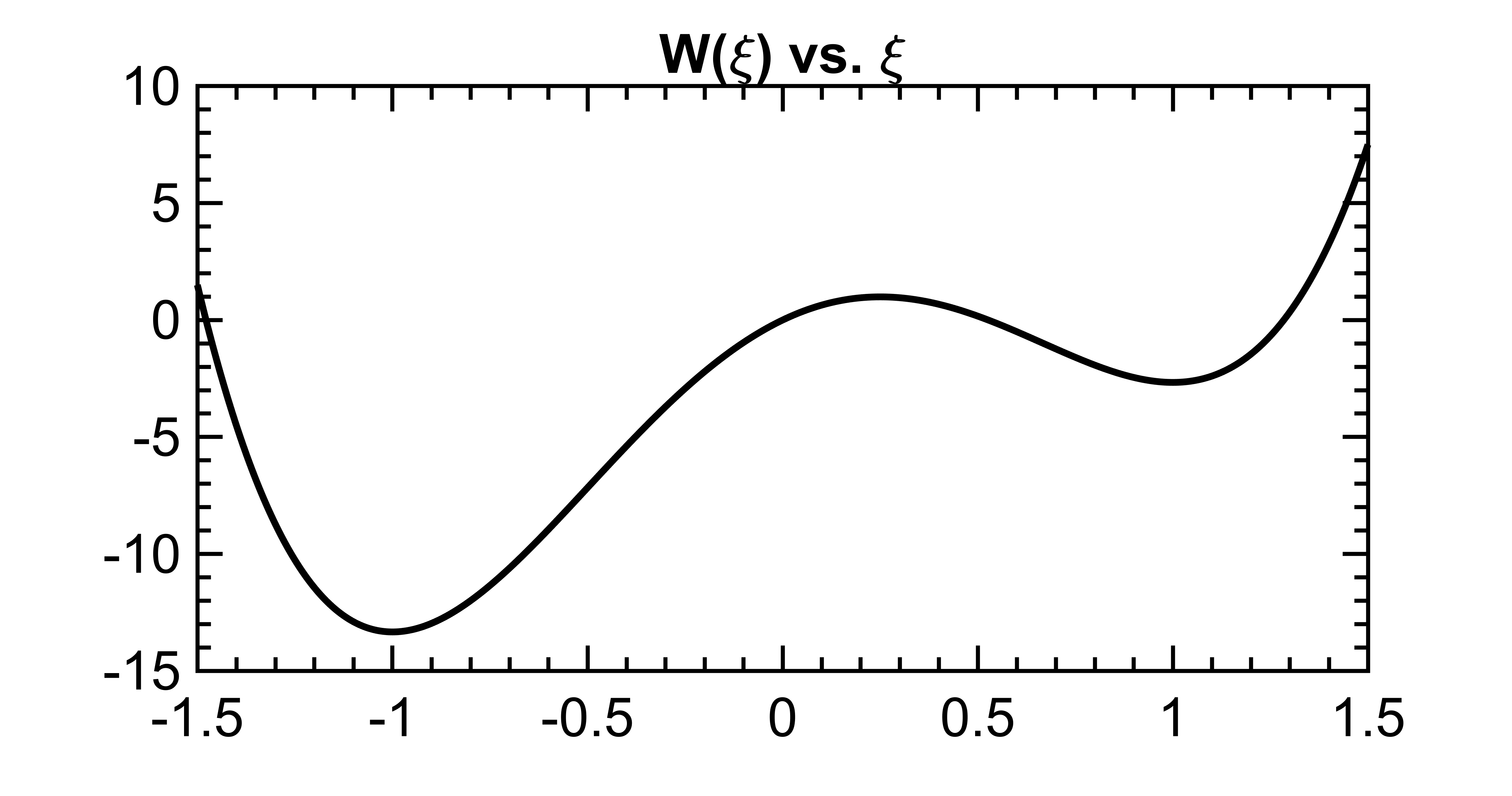
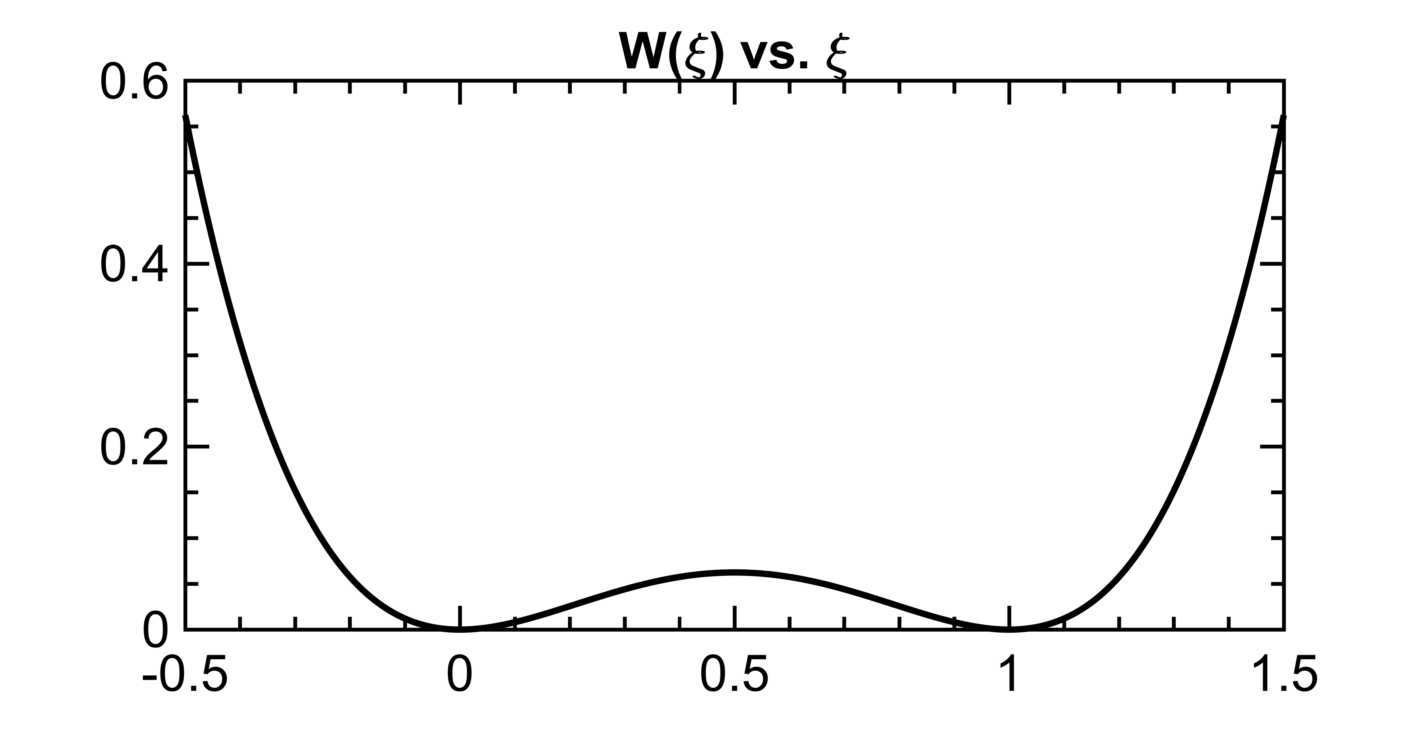
Figure 1: The double well potentials used in the Allen-Cahn Eq. 45 and Cahn-Hilliard Eq. 47 equations: One with unequal depth wells and the other with equal depth wells.

Figure 2: The initial condition (black) and the solution at final time (gray) in the numerical convergence study on the 1D Allen-Cahn equation Eq. 45 with a potential that has unequal depth wells.

We start with the Allen-Cahn equation

(45) $$u_{t}=\Delta u-W^{\prime}(u)$$

where $W:\mathbb{R}\to\mathbb{R}$ is a double-well potential. This corresponds to gradient flow for the energy

(46) $$E(u)=\int\frac{1}{2}\|\nabla u\|^{2}+W(u)\,dx$$

with respect to the $L^{2}$ inner product.

First, we consider equation Eq. 45 in one space dimension, with the potential $W(u)=8u-16u^{2}-\frac{8}{3}u^{3}+8u^{4}$. This is a double well potential with unequal depth wells; see Fig. 1. In this case, equation Eq. 45 is well-known to possess traveling wave solutions on $x\in\mathbb{R}$, see Fig. 2. We choose the initial condition $u(x,0)=\tanh(4x+20)$; the exact solution is then $u_{*}(x,t)=\tanh(4x+20-8t)$. The computational domain is $x\in[-10,10]$, discretized into a uniform grid of $8193$ points. We approximate the solution on $\mathbb{R}$ by using the Dirichlet boundary conditions $u(\pm 10,t)=\pm 1$: The domain size is large enough that the mismatch in boundary conditions do not substantially contribute to the error in the approximate solution over the time interval $t\in[0,5]$. We use $E_{1}(u)=\int\frac{1}{2}|\nabla u|^{2}dx$ and $E_{2}(u)=\int W(u)dx$. Table 2 tabulates the error in the computed solution at time $T=5$ for our two new schemes.

Number of
time steps	$2^{9}$	$2^{10}$	$2^{11}$	$2^{12}$	$2^{13}$
$L^{2}$ error (2nd order)	2.08e-01	5.96e-02	1.61e-02	4.22e-03	1.08e-03
Order	-	1.81	1.89	1.94	1.97
$L^{2}$ error (3rd order)	2.06e-03	3.26e-04	4.68e-05	6.32e-06	8.33e-07
Order	-	2.66	2.80	2.89	2.92

Table 2: The new second Eq. 32 and third Eq. 33 order accurate, conditionally stable schemes Eq. 9 on the one-dimensional Allen-Cahn equation Eq. 45 with a traveling wave solution.

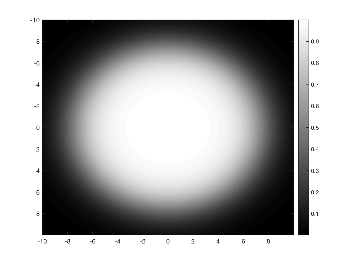
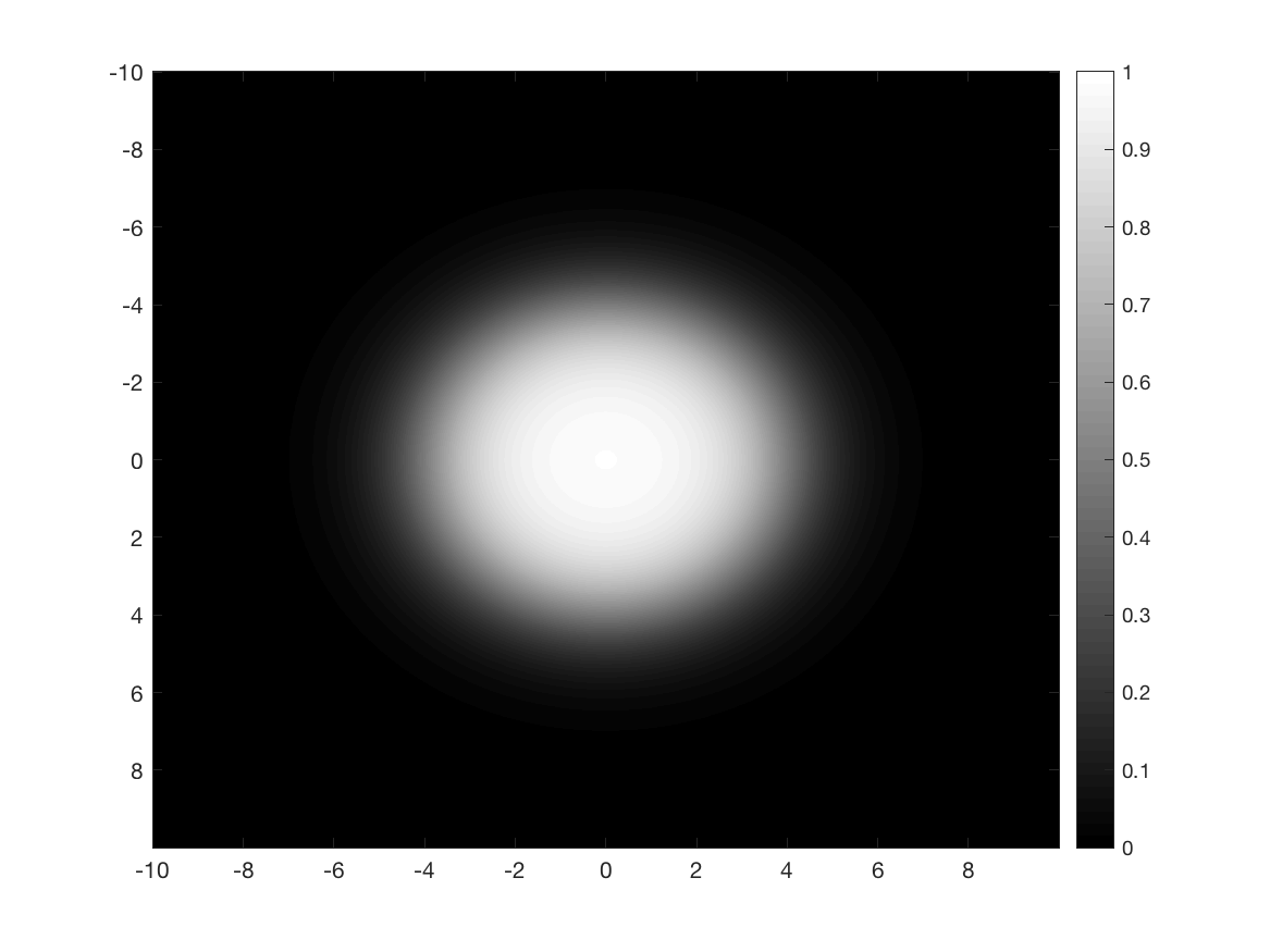
Figure 3: Initial condition and the solution at final time for the 2D Allen-Cahn equation with a potential that has equal depth wells.

Next, we consider the Allen-Cahn equation Eq. 45 in two space-dimensions, with the potential $W(u)=u^{2}(1-u)^{2}$ that has equal depth wells; see Fig. 1. We take the initial condition $u(x,y,0)=\frac{1}{1+\exp[-(7.5-\sqrt{x^{2}+y^{2}})]}$ on the domain $x\in[-10,10]^{2}$, and impose periodic boundary conditions. Once again we use $E_{1}(u)=\int\frac{1}{2}\|\nabla u\|^{2}dx$ and $E_{2}(u)=\int W(u)dx$. As a proxy for the exact solution of the equation with this initial data, we compute a very highly accurate numerical approximation $u_{*}(x,y,t)$ via the following second order accurate in time, semi-implicit, multi-step scheme  [1] on an extremely fine spatial grid and take very small time steps:

$$\frac{3}{2}u^{n+1}-2u^{n}+\frac{1}{2}u^{n-1}=k\Delta u^{n+1}-k(2W^{\prime}(u^{n})-W^{\prime}(u^{n-1})).$$

Table 3 show the errors and convergence rates for the approximate solutions computed by our new multi-stage schemes.

Number of
time steps	$2^{8}$	$2^{9}$	$2^{10}$	$2^{11}$	$2^{12}$
$L^{2}$ error (2nd order)	3.62e-05	9.07e-06	2.27e-06	5.68e-07	1.41e-07
Order	-	2.00	2.00	2.00	2.00
$L^{2}$ error (3rd order)	2.35e-05	3.18e-06	4.15e-07	5.29e-08	6.24e-09
Order	-	2.88	2.94	2.97	3.08

Table 3: The new second Eq. 32 and third Eq. 33 order accurate, conditionally stable schemes Eq. 9 on the two-dimensional Allen-Cahn equation Eq. 45 with a potential that has equal depth wells.

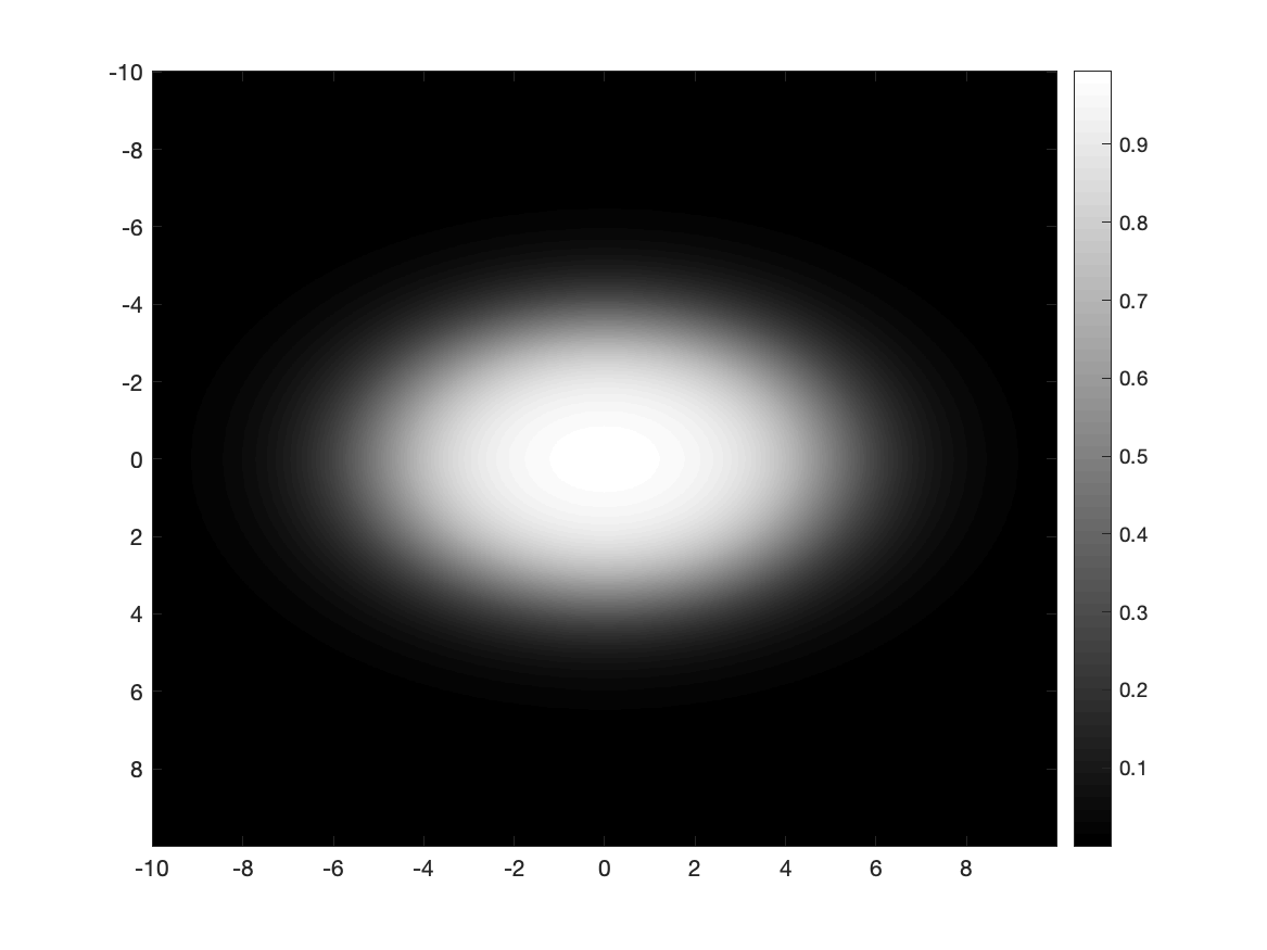
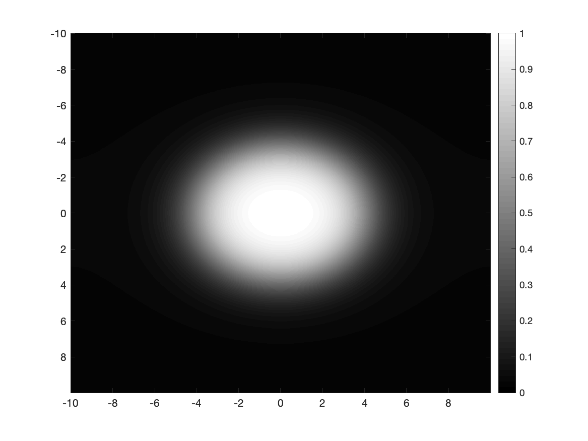
Figure 4: Initial condition and the solution at final time for the 2D Cahn-Hillard equation with a potential that has equal depth wells.

For our next example, we consider the Cahn-Hilliard equation

(47) $$u_{t}=-\Delta\big{(}\Delta u-W^{\prime}(u)\big{)}$$

where we take $W$ to be the double well potential $W(u)=u^{2}(1-u)^{2}$ with equal depth wells and impose periodic boundary conditions. This flow is also gradient descent for energy Eq. 46, but with respect to the $H^{-1}$ inner product:

$$\langle u\,,v\,\rangle=\int u\Delta^{-1}v\,dx.$$

Starting from the initial condition $u(x,y,0)=\frac{1}{1+\exp[-(5-\sqrt{x^{2}+y^{2}})]}$, we computed a proxy for the “exact” solution once again using the second order accurate, semi-implicit multi-step scheme from [1]:

$$\frac{3}{2}u^{n+1}-2u^{n}+\frac{1}{2}u^{n-1}=-k\Delta[\Delta u^{n+1}-(2W^{\prime}(u^{n})-W^{\prime}(u^{n-1}))]$$

where the spatial and temporal resolution was taken to be high to ensure the errors are small. Table 4 show the errors and convergence rates for the approximate solutions computed by our new multi-stage schemes.

Number of
time steps	$2^{7}$	$2^{8}$	$2^{9}$	$2^{10}$	$2^{11}$
$L^{2}$ error (2nd order)	6.20e-04	1.92e-04	5.59e-05	1.55e-05	4.09e-06
Order	-	1.69	1.78	1.85	1.92
$L^{2}$ error (3rd order)	6.45e-06	1.35e-06	2.51e-07	4.15e-08	7.20e-09
Order	-	2.25	2.43	2.60	2.53

Table 4: The new second Eq. 32 and third Eq. 33 order accurate, conditionally stable schemes Eq. 9 on the two-dimensional Cahn-Hilliard equation Eq. 47 with a potential that has equal depth wells.

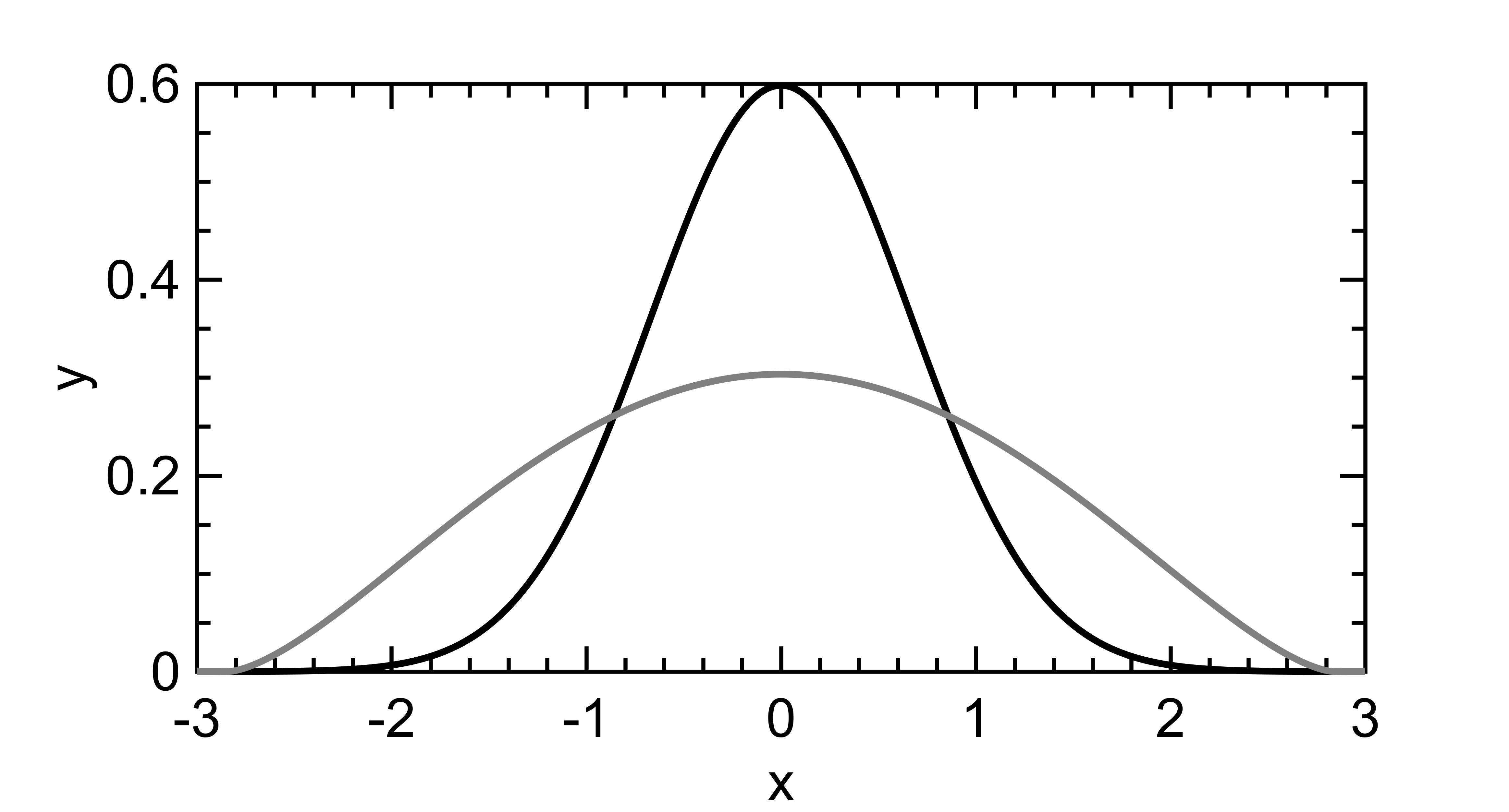
Figure 5: The initial condition (black) and the solution at final time (gray) in the numerical convergence study on the PME

As a final example we do the following porous medium equation:

(48) $$u_{t}=\Delta u^{5/3}$$

Under the $H^{-1}$ inner product, Eq. 48 is gradient flow for the energy

$$E(u)=\frac{3}{8}\int u^{8/3}dx.$$

Our initial data is

(49) $$u(x,0)=\frac{3}{2\sqrt{2\pi}}\exp\bigg{(}-\frac{9x^{2}}{8}\bigg{)}$$

in $x\in[-3,3]$ with derivative zero Neumann boundary conditions. We run the simulation for $T=1$. See Fig. 5 for our initial and final curve. We generate the “true” solution using the L-stable (but not energy stable) TR-BDF2 method with a high spatial and temporal resolution. See Table 5 for results.

Number of
time steps	$2^{12}$	$2^{13}$	$2^{14}$	$2^{15}$	$2^{16}$
$L^{2}$ error (2nd order)	1.91e-06	6.85e-07	2.26e-07	6.90e-08	1.97e-08
Order	-	1.48	1.60	1.71	1.81
$L^{2}$ error (3rd order)	2.21e-07	5.69e-08	1.26e-08	2.41e-09	4.13e-10
Order	-	1.96	2.18	2.38	2.54

Table 5: The new second Eq. 32 and third Eq. 33 order accurate, conditionally stable schemes Eq. 9 on the porous medium equation

5.2 Gradient Flow For Solution Dependent Inner Product

Our first example we present in this section is the heat equation, $u_{t}=\Delta u$, but with a different energy. Under the Wasserstein metric (denoted as $W_{2}$), the heat equation is a gradient flow for the negative entropy [7]:

(50) $$E(u)=\int u\log(u)dx.$$

However the minimization

$$\operatorname*{arg\,min}_{u}E(u)+\frac{1}{2k}W_{2}^{2}(u,u_{n})$$

is a difficult optimization problem. On the other hand, we can approximate the the Wasserstein metric, $W_{2}(u,v)$, with

(51) $$\langle u-v,\mathcal{L}(u)^{-1}(u-v)\rangle_{L^{2}}\text{ where }\mathcal{L}(u)=-\nabla\cdot u\nabla$$

when $u$ and $v$ are near each other. Indeed

$$-\mathcal{L}(u)\nabla_{L^{2}}E(u)=\nabla\cdot u\nabla(\log(u)+1)=\Delta u.$$

Thus, we can alternatively think of the heat equation as minimizing movements on negative entropy with respect to the solution dependent inner product Eq. 51 and therefore use Algorithm 1 and Algorithm 2 to evolve the heat equation while decreasing the negative entropy Eq. 50 at every step.

We use the exact solution $u(x,t)=\cos(\pi x)\exp(-t\pi^{2})+2$ as our test with domain $x\in[0,1]$ using derivative zero Neumann boundary conditions. Our initial data is $u(x,0)$ and we run the simulation to final time $T=\frac{1}{10}$. We use $E_{1}(u)=\frac{1}{2}\int u^{2}dx$ and $E_{2}(u)=\int u\log(u)dx-\frac{1}{2}\int u^{2}dx$ in Eq. 9 so at every step we are solving a linear systems of equation. We run simulation for $T=\frac{1}{10}$. See Table 6 for results.

Number of
time steps	$2^{3}$	$2^{4}$	$2^{5}$	$2^{6}$	$2^{7}$
$L^{2}$ error (2nd order)	1.06e-03	3.11e-04	8.58e-05	2.27e-05	5.85e-06
Order	-	1.77	1.86	1.92	1.96
$L^{2}$ error (3rd order)	1.00e-05	1.57e-06	2.20e-07	3.04e-08	4.29e-09
Order	-	2.69	2.82	2.87	2.83

Table 6: The new second (Algorithm 1) and third (Algorithm 2) order accurate, conditionally stable schemes for gradient flows with solution dependent inner product on the heat equation with Wasserstein metric.

The next example is the porous medium equation in one dimension. The energy is

$$E(u)=\frac{3}{2}\int u^{5/3}dx$$

under the Wasserstein metric. As with the heat equation, we can again replace the Wasserstein metric with Eq. 51. We will let $E_{1}(u)=E(u)$ and $E_{2}(u)=0$. We use the same test as in the $H^{-1}$ gradient flow porous medium equation (see Eq. 49 and accompanying explanation). We present the results of the porous medium equation test with movement limiter Eq. 51 in Table 7.

Number of
time steps	$2^{4}$	$2^{5}$	$2^{6}$	$2^{7}$	$2^{8}$
$L^{2}$ error (2nd order)	2.69e-04	6.10e-05	1.49e-05	3.71e-06	9.25e-07
Order	-	2.14	2.04	2.01	2.00
$L^{2}$ error (3rd order)	2.88e-0	3.17e-06	3.72e-07	4.53e-08	5.50e-09
Order	-	3.18	3.09	3.04	3.04

Table 7: The new second and third order accurate, unconditionally stable schemes (see Remark 4.1) for gradient flows with solution dependent inner product on the porous medium equation with the linearized Wasserstein metric.

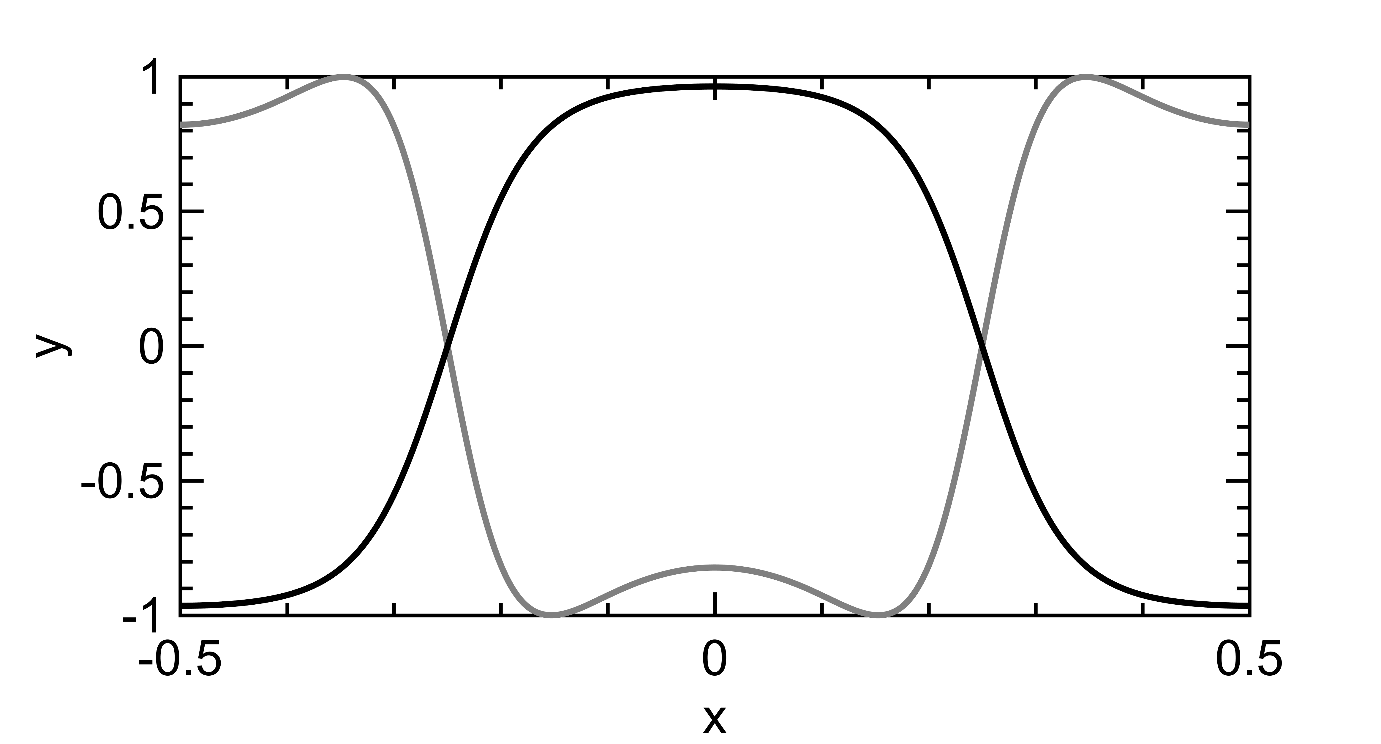
Figure 6: Initial condition (black) and the solution at final time (gray) for the 1D Cahn-Hillard with variable mobility and forcing term example.

For our final example, we consider the Cahn-Hilliard equation with variable mobility and a forcing term:

(52) $$u_{t}=-\nabla\cdot\mu(u)\nabla\big{(}\epsilon^{2}\Delta u-W^{\prime}(u)-F(x)\big{)}$$

where we take $W$ to be the double well potential $W(u)=(1-u^{2})^{2}$ with equal depth wells, the forcing term to be $F(x)=\tanh\big{(}\frac{\cos(2\pi x)}{10\epsilon}\big{)}$ and the mobility to be $\mu(u)=(1-\epsilon)(1-u^{2})^{2}+\epsilon$ to avoid degeneracy in the PDE. This flow is gradient descent for energy

$$E(u)=\int\frac{\epsilon^{2}}{2}\|\nabla u\|^{2}+W(u)+uF(x)\,dx,$$

with respect to the solution dependent inner product

(53) $$\langle u-v,\mathcal{L}(u)^{-1}(u-v)\rangle_{L^{2}}\text{ where }\mathcal{L}(u)=-\nabla\cdot\mu{(u)}\nabla.$$

For our example, we take $\epsilon=\frac{1}{20}$ and starting from the initial condition

$$u(x,0)=\tanh\bigg{(}\frac{\cos(2\pi x)}{10\epsilon}\bigg{)}$$

on the domain $x\in[-\frac{1}{2},\frac{1}{2}]^{2}$, and impose periodic boundary conditions. We run the PDE until time $T=\frac{1}{8}$. We computed a proxy for the “exact” solution using the following second order BDF/AB scheme:

$$3u^{n+1}+2k\epsilon^{2}\Delta^{2}u^{n+1}=4u^{n}-u^{n-1}+4\big{(}k\epsilon^{2}\Delta^{2}u^{n}-k\nabla\cdot\mu(u^{n})\nabla[\epsilon^{2}\Delta u^{n}-W^{\prime}(u^{n})]\big{)}\\ -2\big{(}k\epsilon^{2}\Delta^{2}u^{n-1}-k\nabla\cdot\mu(u^{n-1})\nabla[\epsilon^{2}\Delta u^{n-1}-W^{\prime}(u^{n-1})]\big{)}$$

where the spatial and temporal resolution were taken to be high to ensure the errors are negligible. See Fig. 6 for plots of the initial condition and the solution at the final time. Table 8 shows the errors and convergence rates for the approximate solutions computed by our new multi-stage schemes.

Number of
time steps	$2^{7}$	$2^{8}$	$2^{9}$	$2^{10}$	$2^{11}$
$L^{2}$ error (2nd order)	4.10e-04	1.29e-04	3.84e-05	1.09e-05	2.96e-06
Order	-	1.67	1.75	1.82	1.88
$L^{2}$ error (3rd order)	1.79e-05	3.68e-06	6.72e-07	1.06e-07	1.42e-08
Order	-	2.28	2.46	2.66	2.90

Table 8: The new second Algorithm 1 and third Algorithm 2 order accurate, conditionally stable schemes for gradient flows with solution dependent inner product on the one-dimensional Cahn-Hilliard equation with variable mobility and forcing term Eq. 52.

6 Conclusion

We presented a new class of implicit-explicit additive Runge-Kutta schemes for gradient flows that are high order and conditionally stable. Additionally, we developed new high order stable schemes for gradient flows on solution dependent inner products. Both of these methods allow us to painlessly increase the order of accuracy of existing schemes for gradient flows without sacrificing stability. We provided many numerical examples of gradient flows, including those that have solution dependent inner product, and have shown that the methods achieve their advertised accuracy.

However, in this paper, we have not developed a systematic approach to coming up with conditionally stable methods of a certain order. In fact, there may exist 2nd and 3rd order methods of fewer stages than given here. Additionally, whether these schemes can be used to achieve arbitrarily high (i.e. $\geq 4$) order in time is unknown. We leave these questions to future work.

Appendix A A Second and Third Order Fully Implicit Methods for Gradient Flows with Solution Dependant Inner Product

Here we layout fully implicit, second and third order algorithms for gradient flows with solution dependant inner product,

$$u_{t}=-\mathcal{L}(u)\nabla E(u).$$

In this case, each substep has form:

(54) $$\bigg{[}\sum^{m-1}_{i=0}\gamma_{m,i}\bigg{]}U_{m}+k\mathcal{L}(u_{*})\nabla_{H}E(U_{m})=\sum^{m-1}_{i=0}\gamma_{m,i}U_{i}.$$

The satisfaction of consistency to the exact solution, Eq. 35, is similar to its semi-implicit counterpart in Section 4. Theorem 2.1 in [12] (which is the special case of this paper’s Theorem 2.1 when $E_{2}=0$) ensures that the coefficients in this section form multistage methods that are energy stable. The exact values for the coefficients for the multistage methods can be found at https://github.com/AZaitzeff/SIgradflow.

A.1 Second order example

The following second order method is unconditionally energy stable. Fix a time step size $k>0$. Set $u_{n}=u_{0}$. To obtain $u_{n+1}$ from $u_{n}$, carry out the following steps:

1. Find $u_{*}$ by solving

   $$u_{*}+\frac{1}{2}k\mathcal{L}_{n}\nabla E(u_{*})=u_{n}$$

2. Find $u_{n+1}$ using Eq. 54 with coefficients

   (55) $$\gamma\approx\left(\begin{array}[]{ccc}5.0&0&0\\ -2.0&6.0&0\\ -2.0&0.22&6.29\\ \end{array}\right).$$

   and $u_{*}$ in $\mathcal{L}(u_{*})$ given by Step 1 of this algorithm.

A.2 Third order example

This third order algorithm is energy stable as long as

$$\mathcal{L}(u)-\frac{1}{72}k^{2}D^{2}\mathcal{L}(u)(w,w)$$

is positive definite for all $u$ and $w$.

Fix a time step size $k>0$. Set $u_{n}=u_{0}$. For convenience, we will denote $D^{2}\mathcal{L}(u_{*})\big{(}\mathcal{L}(u_{*})\nabla E(u_{*}),\mathcal{L}(u_{*})\nabla E(u_{*})\big{)}$ as $D^{2}\mathcal{L}(u_{*})$ and $MS(\tilde{k},\mathcal{L}(u_{*}),\tilde{u},\gamma)$ as $U_{M}$ in the multistage algorithm

$$\bigg{[}\sum^{m-1}_{i=0}\gamma_{m,i}\bigg{]}U_{m}+\tilde{k}\mathcal{L}(u_{*})\nabla_{H}E(U_{m})=\sum^{m-1}_{i=0}\gamma_{m,i}U_{i}.$$

with time step $\tilde{k}$, operator $\mathcal{L}(u_{*})$, $U_{0}=\tilde{u}$ and coefficients $\gamma$. To obtain $u_{n+1}$ from $u_{n}$, carry out the following steps:

1. Set $\gamma=\left(1\right)$ and $u_{*_{1}}=MS\Big{(}\frac{1}{6}k,\mathcal{L}(u_{n}),u_{n},\gamma\Big{)}$.

2. Set

   (62) $$\gamma\approx\left(\begin{array}[]{cccccc}11.17&0&0&0&0&0\\ -7.5&19.43&0&0&0&0\\ -1.05&-4.75&13.98&0&0&0\\ 1.8&0.05&-7.83&13.8&0&0\\ 6.2&-7.17&-1.33&1.63&11.52&0\\ -2.83&4.69&2.46&-11.55&6.68&11.95\\ \end{array}\right)$$

   and

   $$\bar{u}=MS\bigg{(}\frac{1}{2}k,\mathcal{L}(u_{*_{1}})-\frac{1}{72}D^{2}\mathcal{L}(u_{*_{1}}),u_{n},\gamma\bigg{)}.$$

3. Set $\gamma=\left(1\right)$ and $u_{*_{2,1}}=MS\Big{(}\frac{2}{5}k,\mathcal{L}(u_{n}),u_{n},\gamma\Big{)}$.

4. Set

   (63) $$\gamma\approx\left(\begin{array}[]{cccc}6.17&0&0&0\\ -0.5&6&0&0\\ -3&2&7&0\\ -3.1&0&2.23&7.40\\ \end{array}\right)$$

   and

   $$u_{*_{2,2}}=MS\bigg{(}\frac{5}{6}k,\mathcal{L}(u_{*_{2,1}}),u_{n},\gamma\bigg{)}.$$

5. Set $\gamma$ to Eq. 62 and then

   $$u_{n+1}=MS\bigg{(}\frac{1}{2}k,\mathcal{L}(u_{*_{2,2}})-\frac{1}{72}D^{2}\mathcal{L}(u_{*_{2,2}}),\bar{u},\gamma\bigg{)}.$$

   .

References

- [1] L. Q. Chen and J. Shen, Applications of semi-implicit Fourier-spectral method to phase field equations, Computer Physics Communications, 108 (1998), pp. 147–158.
- [2] W. Chen, C. Wang, X. Wang, and S. M. Wise, Positivity-preserving, energy stable numerical schemes for the Cahn-Hilliard equation with logarithmic potential, Journal of Computational Physics: X, 3 (2019), p. 100031.
- [3] F. Del Teso, J. Endal, and E. R. Jakobsen, Robust numerical methods for nonlocal (and local) equations of porous medium type. part ii: Schemes and experiments, SIAM Journal on Numerical Analysis, 56 (2018), pp. 3611–3647.
- [4] C. Duan, C. Liu, C. Wang, and X. Yue, Numerical methods for porous medium equation by an energetic variational approach, Journal of Computational Physics, 385 (2019), pp. 13–32.
- [5] D. J. Eyre, Unconditionally gradient stable time marching the Cahn-Hilliard equation, MRS Online Proceedings Library Archive, 529 (1998).
- [6] D. Han and X. Wang, A second order in time, uniquely solvable, unconditionally stable numerical scheme for Cahn–Hilliard–Navier–Stokes equation, Journal of Computational Physics, 290 (2015), pp. 139–156.
- [7] R. Jordan, D. Kinderlehrer, and F. Otto, The variational formulation of the Fokker–Planck equation, SIAM journal on mathematical analysis, 29 (1998), pp. 1–17.
- [8] C. A. Kennedy and M. H. Carpenter, Additive Runge–Kutta schemes for convection–diffusion–reaction equations, Applied Numerical Mathematics, 44 (2003), pp. 139–181.
- [9] L. Pareschi and G. Russo, Implicit–explicit Runge–Kutta schemes and applications to hyperbolic systems with relaxation, Journal of Scientific Computing, 25 (2005), pp. 129–155, https://doi.org/10.1007/s10915-004-4636-4, https://doi.org/10.1007/s10915-004-4636-4.
- [10] J. Shin, H. G. Lee, and J.-Y. Lee, Unconditionally stable methods for gradient flow using convex splitting Runge–Kutta scheme, Journal of Computational Physics, 347 (2017), pp. 367–381.
- [11] M. Westdickenberg and J. Wilkening, Variational particle schemes for the porous medium equation and for the system of isentropic euler equations, ESAIM: Mathematical Modelling and Numerical Analysis, 44 (2010), pp. 133–166.
- [12] A. Zaitzeff, S. Esedoglu, and K. Garikipati, Variational extrapolation of implicit schemes for general gradient flows, 2019, https://arxiv.org/abs/1908.10246.
- [13] E. Zharovsky, A. Sandu, and H. Zhang, A class of implicit-explicit two-step Runge–Kutta methods, SIAM Journal on Numerical Analysis, 53 (2015), pp. 321–341.