Jumps and Coalescence in the Continuum: a Numerical Study

Abstract.

The dynamics is studied of an infinite continuum system of jumping and coalescing point particles. In the course of jumps, the particles repel each other whereas their coalescence is free. As the equation of motion we take a kinetic equation, derived by a scaling procedure from the microscopic Fokker-Planck equation corresponding to this kind of motion. The result of the paper is the numerical study (by the Runge-Kutta method) of the solutions of the kinetic equation revealing a number of interesting peculiarities of the dynamics and clarifying the particular role of the jumps and the coalescence in the system’s evolution. Possible nontrivial stationary states are also found and analyzed.

1. Introduction

In a broader sense, a typical kinetic equation is a nonlinear integro-differential equation describing the temporal evolution of the density function of a large (infinite) system of ‘particles’. At this level of description, the individual particles are not taken into account and the system is considered as a medium, entirely characterized by its aggregate parameters like density. A prototype example is the celebrated Boltzmann equation [10] devised by Ludwig Boltzmann in 1872 to describe large systems of physical particles. Since then this approach has received various applications ranging from the theory of multiple-lane vehicular traffic [23] to the description of evolving ecological systems [1, 7, 19, 20]. Usually, kinetic equations are devised with the help of phenomenological or heuristic arguments, and thus are only loosely related to so called ‘first principles’, e.g., by taking into account appropriate conservation laws and symmetries. Due to Bogoliubov’s pioneering works [6], see also [9], it has become clear that the Boltzmann equation can be derived (by a certain decoupling or truncating procedure) from an infinite chain of linear equations – the BBGKY hierarchy – that describes the microscopic evolution of a particle system, see e.g., [25]. This approach was then extended to deriving kinetic equations describing ecological systems from the corresponding microscopic equations of their random evolution [13, 19].

In view of various applications – also but not only those mentioned above – there exists a permanent interest to the evolution of statistically large systems in the course of which the constituents can merge. As an example, in ecological models merging can be used to describe the predation [8]. The Arratia flow [2] provides an example of the motion of this sort. Its recent study can be found in [5, 14, 15, 18] and in the works quoted therein. In Arratia’s model, an infinite number of Brownian particles move in $\mathds{R}$ independently up to their collision, then merge and move together as single particles. Correspondingly, the description of this motion is performed in terms of diffusion processes. In an accompanying work [17], we propose an alternative model of this kind. In this model, an infinite system of point particles located in $\mathds{R}^{d}$, $d\geq 1$ undergo random evolution consisting in the following two elementary acts, see Fig. 1:

• Two particles (located at $x$ and $y$) merge into a particle (located at $z$) with intensity (probability per time) $c_{1}(x,y;z)$ – independent of the remaining particles. Thereafter, this new particle participates in the motion.

• Similarly as in the Kawasaki model [4], single particles perform random jumps with repulsion acting on the target point.

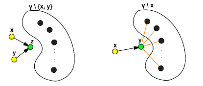
Figure 1. Elementary acts of evolution

For the microscopic description of this model, as the phase space one employs the set $\Gamma$ of all locally finite configurations $\gamma\subset\mathds{R}^{d}$, see [4, 16] and the next section. The microscopic states of the system are then probability measures on $\Gamma$ the set of which is denoted by $\mathcal{P}(\Gamma)$. The evolution of states $\mu_{0}\to\mu_{t}$ is obtained by solving the Fokker-Planck equation. The main result of [17] is the proof of the existence of the evolution of this type for a bounded time horizon. However, by virtue of this result the most important and interesting details of the collective motion of the system remain unrevealed. The aim of the present work is to study the mentioned model numerically by employing the corresponding kinetic equation derived from the microscopic theory developed in [17]. The main questions we address here are: (a) which peculiarities of the motion are related to each of the mentioned elementary acts of the evolution; (b) what is the role of the interaction (repulsion) in the possible appearance of a spatial heterogeneity in the system. In a sense, this our research is a continuation of the study in [21] – by similar numerical methods – of the spatial ecological model the existential problems of which were settled in [16].

2. Theoretical Background

As mentioned above, the microscopic theory of our model is based on the Fokker-Planck equation. The mesoscopic description employs a kinetic equation obtained from the corresponding microscopic evolution equations by a scaling procedure, cf. [3, 13]. Its solutions are evolving particle densities that will be the objects of our numerical study.

2.1. Microscopic description

The phase space of the dynamics which we study is the set of locally finite subsets of $\mathds{R}^{d}$ – configurations – defined as follows

$$\Gamma=\{\gamma\subset\mathds{R}^{d}:|\Lambda\cap\gamma|<\infty\text{ for any compact }\Lambda\subset\mathds{R}^{d}\},$$

where $|\cdot|$ denotes cardinality. It is equipped with the vague (weak-hash) topology see e.g., [4, 13]) and the corresponding Borel $\sigma$-field $\mathcal{B}(\Gamma)$. This allows one to employ probability measures $\mu$ defined on $(\Gamma,\mathcal{B}(\Gamma))$ as states of the considered system. The set of all such measures is $\mathcal{P}(\Gamma)$. The evolution of the model is described by the Fokker-Planck equation

$$\mu_{t}(F)=\mu_{0}(F)+\int_{0}^{t}\mu_{s}(LF)ds,$$ (2.1)

in which $F:\Gamma\to\mathds{R}$ is an appropriate test function, $\mu(F):=\int_{\Gamma}Fd\mu$, and the operator $L$ specifies the model. In our case, it is

$$(LF)(\gamma)=\sum\limits_{\{x,y\}\subset\gamma}\ \int\limits_{\mathds{R}^{d}}c_{1}(x,y;z)\Big{(}F\big{(}\gamma\backslash\{x,y\}\cup z\big{)}-F(\gamma)\Big{)}dz$$ (2.2)

$$+\sum\limits_{x\in\gamma}\ \int\limits_{\mathds{R}^{d}}\tilde{c}_{2}(x,y;\gamma)\Big{(}F\big{(}\gamma\backslash x\cup y\big{)}-F(\gamma)\Big{)}dy.$$

Here $c_{1}\geq 0$ is the intensity of the coalescence of the particles located at $x$ and $y$ into a new particle located at $z$. Note that $c_{1}$ does not depend on the elements of $\gamma$ other than $x$ and $y$. For simplicity, we assume that $c_{1}(x,y;z)=c_{1}(y,x;z)=c_{1}(x+u,y+u;z+u)$ for all $u\in\mathds{R}^{d}$, i.e., $c_{1}$ is translation invariant. For more general versions of this model – that describe also coalescence with interactions – see [22]. The second summand in (2.2) describes jumps performed by the particles. Similarly as in [4], we take it in the form

$$\tilde{c}_{2}(x,y;\gamma)=c_{2}(x-y)\prod\limits_{u\in\gamma\backslash x}e^{-\phi(y-u)},$$

with $\phi$ and $c_{2}$ being the repulsion potential and the jump kernel, respectively. By these assumptions the model is translation invariant. The functions $c_{1}$, $c_{2}$ and $\phi$ take non-negative values and are supposed to satisfy the following conditions:

$$\int\limits_{(\mathds{R}^{d})^{2}}c_{1}(x_{1},x_{2};x_{3})dx_{i}dx_{j}=\langle c_{1}\rangle\ <\infty,$$ (2.3)

$$c_{1}^{\text{max}}:=\sup_{x,y\in\mathds{R}^{d}}\int\limits_{\mathds{R}^{d}}c_{1}(x,y;z)dz<\infty,$$

$$\langle c_{2}\rangle\ :=\int\limits_{\mathds{R}^{d}}c_{2}(x)dx<\infty,\quad\langle\phi\rangle:=\int\limits_{\mathds{R}^{d}}\phi(x)dx<\infty,$$

$$|\phi|:=\sup_{x\in\mathds{R}^{d}}\phi(x)<\infty.$$

As the operator (2.2) is quite complex, the direct study of the Fokker-Planck equation (2.1) is rather inaccessible. Instead, in [17] we realized the following construction. For $t<T$ (with some $T<\infty$) and $\mu_{0}$ belonging to a certain subset of $\mathcal{P}(\Gamma)$, the evolution $\mu_{0}\to\mu_{t}$ was obtained as the evolution $k_{0}\to k_{t}$ of the correlation functions corresponding to these states. The basic aspects of this construction can be outlined as follows. Let $\varOmega$ stand for the set of all compactly supported continuous functions $\omega:\mathds{R}^{d}\to(-1,0]$. Set

$$F^{\omega}(\gamma)=\prod_{x\in\gamma}(1+\omega(x)),\qquad\omega\in\varOmega.$$

Each $F^{\omega}$ is bounded and continuous, hence integrable for each $\mu$. Moreover, the collection $\{F^{\omega}:\omega\in\varOmega\}$ is a measure-defining class, cf. [11, page 79]. The set of measures $\mathcal{P}_{\rm exp}\subset\mathcal{P}(\Gamma)$ we will work with is defined by the condition that its members enjoy the following property: the map $\varOmega\ni\omega\mapsto\mu(F^{\omega})\in\mathds{R}$ can be continued to an exponential type entire function defined on $L^{1}(\mathds{R}^{d})$. Then, for $\mu\in\mathcal{P}_{\rm exp}$, we set $B_{\mu}(\omega)=\mu(F^{\omega})$ and derive $\widetilde{L}$ from $L$ according to the rule $(\widetilde{L}B_{\mu})(\omega)=\mu(LF^{\omega})$. Thereafter, we construct the evolution $B_{\mu_{0}}\to B_{t}$ by solving the corresponding evolution equation. The next (and the hardest) part of this scheme is to prove that $B_{t}=B_{\mu_{t}}$ for a unique $\mu_{t}\in\mathcal{P}_{\rm exp}$. The advantage of using $\mathcal{P}_{\rm exp}$ is that, for each of its members, the function $B_{\mu}$ admits the representation

$$B_{\mu}(\omega) = 1+\sum_{n=1}^{\infty}\frac{1}{n!}\int_{(\mathds{R}^{d})^{n}}k^{(n)}_{\mu}(x_{1},\dots,x_{n})\omega(x_{1})\cdots\omega(x_{n})dx_{1}\cdots dx_{n}.$$ (2.4)

Here $k^{(n)}_{\mu}$ is the $n$-th order correlation function of state $\mu$. It satisfies the Ruelle bound [24]

$$0\leq k^{(n)}_{\mu}(x_{1},\dots,x_{n})\leq\varkappa^{n},$$

with an appropriate $\varkappa>0$. Since each $k^{(n)}$ is defined by (2.4) only Lebesgue-almost everywhere, the latter estimate yields $k^{(n)}\in L^{\infty}((\mathds{R}^{d})^{n})$, and $k^{(n)}$, $n\geq 2$ is symmetric with respect to the interchange of $x_{i}$. For a compact $\Lambda\subset\mathds{R}^{d}$,

$$\mu(N_{\Lambda})=\int_{\Gamma}N_{\Lambda}(\gamma)\mu(d\gamma)=\int_{\Lambda}k_{\mu}^{(1)}(x)dx$$

is the expected value of the number of points contained in $\Lambda$ if the system is in state $\mu$. Here $N_{\Lambda}(\gamma)=|\gamma\cap\Lambda|$ is the number of the elements of $\gamma$ contained in $\Lambda$. That is, $k_{\mu}^{(1)}$ is the particle density in state $\mu$. Note that $\mu(N_{\Lambda})$ may be infinite for a non-compact $\Lambda$, which would indicate that the system is infinite in state $\mu$. By the estimate above we have that

$$\|k^{(n)}_{\mu}\|_{L^{\infty}((\mathds{R}^{d})^{n})}\leq\varkappa^{n},\qquad n\in\mathds{N}.$$ (2.5)

Let $\Gamma_{0}$ stand for the set of all finite configurations. It is a measurable subset of $\Gamma$, equipped with the topology induced thereon by the vague topology of $\Gamma$. The elements of $\Gamma_{0}$ will usually be denoted by $\eta$. Thus, $\eta=\{x_{1},\dots,x_{n}\}$ with distinct $x_{j}$, and $n=|\eta|$ is the number of points in $\eta$. Let $k_{\mu}:\Gamma_{0}\to\mathds{R}$ be defined by $k_{\mu}(\eta)=k^{(n)}_{\mu}(x_{1},\dots,x_{n})$ for $\eta$ as above. This is the correlation function of state $\mu\in\mathcal{P}_{\rm exp}$ which characterizes it in a complete way. For instance, for a Poisson measure $\pi_{\rho}$ with density $\rho:\mathds{R}^{d}\to[0,+\infty)$ we have

$$k_{\pi_{\rho}}(\eta)=\prod_{x\in\eta}\rho(x).$$ (2.6)

That is, $\pi_{\rho}$ is completely characterized by its density (intensity function) $\rho$, cf. [11, page 45]. By (2.5) we conclude that $k_{\mu}\in\mathcal{K}_{\vartheta}$ with $\vartheta=\log\varkappa$ and $\mathcal{K}_{\vartheta}$ being a Banach space of such maps equipped with the norm

$$\|k\|_{\vartheta}:=\sup_{n\geq 0}\bigg{(}e^{-n\vartheta}\|k^{(n)}_{\mu}\|_{L^{\infty}((\mathds{R}^{d})^{n})}\bigg{)}.$$

Then the states $\mu_{t}\in\mathcal{P}_{\rm exp}$ satisfy the Fokker-Planck equation (2.1) with $L$ given in (2.2) and $F=F^{\omega}$ if their correlation functions $k_{t}$ satisfy

$$\frac{d}{dt}k_{t}=L^{\Delta}k_{t},\qquad k_{t}|_{t=0}=k_{\mu_{0}},$$ (2.7)

which, in fact, is an infinite chain of equations for $k_{t}^{(n)},n\in\mathds{N}$. In (2.7), $L^{\Delta}$ has the form, cf. [22],

$$L^{\Delta}=L_{1}^{\Delta}+L_{2}^{\Delta}.$$

Here $L_{1}^{\Delta}=L_{11}^{\Delta}+L_{12}^{\Delta}+L_{13}^{\Delta}+L_{14}^{\Delta}$ is the part responsible for the coalescence whereas $L_{2}^{\Delta}=L_{21}^{\Delta}+L_{22}^{\Delta}$ describes the jumps. Their summands are:

$$(L^{\Delta}_{11}k)(\eta)=\ \ \frac{1}{2}\int\limits_{(\mathds{R}^{d})^{2}}\sum\limits_{z\in\eta}c_{1}(x,y;z)k(\eta\backslash z\cup\{x,y\})dxdy,$$

$$(L^{\Delta}_{12}k)(\eta)=-\frac{1}{2}\int\limits_{(\mathds{R}^{d})^{2}}\sum\limits_{x\in\eta}c_{1}(x,y;z)k(\eta\cup y)dydz,$$

$$(L^{\Delta}_{13}k)(\eta)=-\frac{1}{2}\int\limits_{(\mathds{R}^{d})^{2}}\sum\limits_{y\in\eta}c_{1}(x,y;z)k(\eta\cup x)dxdz,$$

$$(L^{\Delta}_{14}k)(\eta)=-\Psi(\eta)k(\eta),\qquad\Psi(\eta):=\int\limits_{\mathds{R}^{d}}\sum\limits_{\{x,y\}\subset\eta}c_{1}(x,y;z)dz,$$

and

$$L^{\Delta}_{21}k(\eta) =\int\limits_{\mathds{R}^{d}}\sum\limits_{y\in\eta}c_{2}(x-y)\prod\limits_{u\in\eta\backslash y}e^{-\phi(y-u)}\ (Q_{y}k)(\eta\backslash y\cup x)dx,$$

$$L^{\Delta}_{22}k(\eta) =-\int\limits_{\mathds{R}^{d}}\sum\limits_{x\in\eta}c_{2}(x-y)\prod\limits_{u\in\eta\backslash x}e^{-\phi(y-u)}\ (Q_{y}k)(\eta)dy,$$

see [17] for more detail. In order to figure out the real meaning of (2.7), let us write down the first two members of this chain of equations. The first one reads

$$\frac{d}{dt}k_{t}^{(1)}(z) = \frac{1}{2}\int_{(\mathds{R}^{d})^{2}}c_{1}(x,y;z)k_{t}^{(2)}(x,y)dxdy$$

$$- \int_{(\mathds{R}^{d})^{2}}c_{1}(z,y;x)k_{t}^{(2)}(z,y)dxdy$$

$$+ \int_{\mathds{R}^{d}}c_{2}(x-z)\left[(Q_{z}k_{t})^{(1)}(x)-(Q_{x}k_{t}^{(1)})(z)\right]dx,$$

where

$$(Q_{x}k_{t})^{(1)}(y) = k_{t}^{(1)}(y)+\sum_{n=1}^{\infty}\frac{1}{n!}\int_{(\mathds{R}^{d})^{n}}k_{t}^{(n+1)}(x_{1},\dots,x_{n},y)$$

$$\times \left(\prod_{j=1}^{n}\left[e^{-\phi(x-x_{j})}-1\right]\right)dx_{1}\cdots dx_{n}.$$

The second member of the chain is

$$\frac{d}{dt}k_{t}^{(2)}(x,y) = \frac{1}{2}\int_{(\mathds{R}^{d})^{2}}\left[c_{1}(u,v;x)k_{t}^{(3)}(y,u,v)+c_{1}(u,v;y)k^{(3)}_{t}(x,u,v)\right]dudv\qquad\qquad$$

$$- \int_{(\mathds{R}^{d})^{2}}\left[c_{1}(x,u;v)k_{t}^{(3)}(x,y,u)+c_{1}(y,u;v)k_{t}^{(3)}(x,y,u)\right]dudv$$

$$- \Psi(x,y)k^{(2)}_{t}(x,y)$$

$$+ \int_{\mathds{R}^{d}}e^{-\phi(x-y)}\left(c_{2}(u-x)(Q_{x}k_{t})^{(2)}(y,u)+c_{2}(u-y)(Q_{y}k_{t})^{(2)}(x,u)\right)du$$

$$- \int_{\mathds{R}^{d}}\left(c_{2}(x-u)e^{-\phi(y-u)}+c_{2}(y-u)e^{-\phi(x-u)}\right)(Q_{u}k_{t})^{(2)}(x,y)du,$$

where

$$\Psi(x,y)=\int_{\mathds{R}^{d}}\left(c_{1}(x,y;z)+c_{1}(y,x;z)\right)dz,$$

and

$$(Q_{z}k_{t})^{(2)}(u,v) = k^{(2)}_{t}(u,v)+\sum_{n=1}^{\infty}\frac{1}{n!}\int_{(\mathds{R}^{d})^{n}}k_{t}^{(n+2)}(u,v,x_{1},\dots,x_{n})$$

$$\times \left(\prod_{i=1}^{n}\left[e^{-\phi(z-x_{i})}-1\right]\right)dx_{1}\cdots dx_{n}.$$

Noteworthy, unlike to the most of such equations, cf. [21, eqs. (1) and (2)], the right-hand sides of (2.1) and (2.1) contain correlation functions of all orders.

Let us now return to studying (2.7). By the very definition of the norms $\|\cdot\|_{\vartheta}$ the Banach spaces $\mathcal{K}_{\vartheta},\vartheta\in\mathds{R}$ constitute an ascending scale of spaces such that $\mathcal{K}_{\vartheta^{\prime}}\hookrightarrow\mathcal{K}_{\vartheta}$ whenever $\vartheta^{\prime}<\vartheta$. Here $\hookrightarrow$ denotes continuous embedding. By mean of the estimates

$$\left|(L^{\Delta}_{1i}k)(\eta)\right| \leq \left(\frac{1}{2}\langle c_{1}\rangle e^{\vartheta}\|k\|_{\vartheta}\right)|\eta|e^{\vartheta|\eta|},\quad i=1,2,3,$$

$$\left|(L^{\Delta}_{14}k)(\eta)\right| \leq \left(\frac{1}{2}c_{1}^{\rm max}\|k\|_{\vartheta}\right)|\eta|(|\eta|-1)e^{\vartheta|\eta|},$$

as well as, cf. [4, eq. (3.18)],

$$\left|(L^{\Delta}_{2}k)(\eta)\right|\leq\left(2\langle c_{2}\rangle\exp\left(\langle\phi\rangle e^{\vartheta}\right)\|k\|_{\vartheta}\right)|\eta|e^{\vartheta|\eta|},$$

one defines bounded linear operators $L^{\Delta}:\mathcal{K}_{\vartheta^{\prime}}\to\mathcal{K}_{\vartheta}$ and then places the Cauchy problem (2.7) into the mentioned scale of Banach spaces. The results of [17] are contained in the following two statements.

Theorem 2.1.

For each $\vartheta_{0}\in\mathds{R}$ and $\vartheta_{*}>\vartheta_{0}$, and for an arbitrary $k_{0}\in\mathcal{K}_{\vartheta_{0}}$, the problem in (2.7) has a unique classical solution $k_{t}\in\mathcal{K}_{\vartheta_{*}}$ on $[0,T)$ with the bound $T=T(\vartheta_{*},\vartheta_{0})$ dependent on $\vartheta_{0}$ and $\vartheta_{*}$.

A priori the solution $k_{t}$ described in Theorem 2.1 need not be a correlation function of any state, which means that the result stated therein has no direct relation to the evolution of states of the system considered. The next statement removes this drawback.

Theorem 2.2.

Let $\mu_{0}\in\mathcal{P}_{\exp}$ be such that $k_{\mu_{0}}\in\mathcal{K}_{\vartheta_{0}}$ and $T(\vartheta_{*},\vartheta_{0})$ be as in Theorem 2.1. Then the evolution $k_{\mu_{0}}\to k_{t}$ described in Theorem 2.1 has the property: for each $t<T(\vartheta_{*},\vartheta_{0})/2$, $k_{t}$ is the correlation function of a unique state $\mu_{t}\in\mathcal{P}_{\exp}$.

The fact that the evolution described in Theorem 2.2 is only local in time stems from technical limitations of the method used in the proof of this statement. We believe that this drawback could be overcome.

2.2. Mesoscopic description

Theorem 2.2 states the existence of the evolution $\mu_{0}\to\mu_{t}$ of the micro-states of our system obtained by solving the Fokker-Plank equation (2.1). In order to get more detailed information regarding this evolution, we pass to the mesoscopic level based on the kinetic equation which we derive now. Its naive (one may say more direct) version can be outlined as follows. As is known, Poisson measures (with correlation functions given in (2.6)) correspond to the states of systems of particles independently distributed over $\mathds{R}^{d}$. Possible dependencies in a state $\mu$ can be captured by the deviations of $k_{\mu}^{(n)}$’s from the corresponding products of $k_{\mu}^{(1)}$’s. In particular, by the truncated second-order correlation function, cf. [12],

$$\tau^{(2)}_{\mu}(x,y)=k^{(2)}_{\mu}(x,y)-k^{(1)}_{\mu}(x)k^{(1)}_{\mu}(y),$$

Thus, a naive truncation (called also moment closure [19]) consists in putting by force

$$k_{t}^{(n)}(x_{1},\dots,x_{n})=k^{(1)}_{t}(x_{1})k^{(1)}_{t}(x_{2})\cdots k^{(1)}_{t}(x_{n}),\qquad n\geq 2,$$

in the right-hand sides of (2.1), (2.1), and forgetting of (2.1) and of the equations for $k_{t}^{(n)}$, $n\geq 3$. In physical language, it corresponds to a so called “mean-field approximation”, cf. [21] where we get out beyond it. After making this ansatz, one obtains a single nonlinear equation, see (2.2) below with $\rho_{t}=k^{(1)}_{t}$ – instead of the infinite chain of linear equations encrypted in (2.7). A more sophisticated version of passing to the kinetic equation in (2.2) is based on the so-called Poisson approximation of the states, in which each $\mu_{t}$ is approximated in a certain way by the Poisson state $\pi_{\rho_{t}}$ with density $\rho_{t}$. Namely, we say that $\mu\in\mathcal{P}_{\rm exp}$ is approximable by $\pi_{\rho}$ (Poisson-approximable), if for some $\vartheta\in\mathds{R}$ there exists a continuous mapping $A:[0,1]\rightarrow\mathcal{K}_{\vartheta}$ such that $A(0)=k_{\pi_{\rho}}$ and $A(1)=k_{\mu}$. The approximation scheme can be depicted as follows

$\mu_{0}$	$\xleftrightarrow[\text{approximation}]{\text{Poisson}}$	$\pi_{\rho_{0}}$	$\rightarrow$	$\rho_{0}$
$\downarrow$ FPE				$\downarrow$ KE
$\mu_{t}$	$\xleftrightarrow[\text{approximation}]{\text{Poisson}}$	$\pi_{\rho_{t}}$	$\leftarrow$	$\rho_{t}$

Its precise formulation is given in the next statement.

Theorem 2.3.

Let $\mu_{0}\in\mathcal{P}_{\exp}$ be approximable by $\pi_{\rho_{0}}$. Then $\mu_{t}$ stated in Theorem 2.2 is approximable by $\pi_{\rho_{t}}$ for $t<T(\vartheta_{*},\vartheta_{0})/2$, with $T(\vartheta_{*},\vartheta_{0})$ as in Theorem 2.1 and $\rho_{t}$ being the solution to kinetic equation (2.2) with initial condition $\rho_{0}$.

The proof of this theorem – quite technical – is essentially based on the method developed in [17]. It will be presented in a separate work. Here we only note that the temporal locality in this statement is also a matter of technical limitations of the method used in the proof of Theorem 2.2.

The kinetic equation corresponding to (2.7) is

$$\frac{d}{dt}\rho_{t}(x) = \frac{1}{2}\int_{(\mathds{R}^{d})^{2}}c_{1}(y,z;x)\rho_{t}(y)\rho_{t}(z)dydz$$

$$- \left(\int_{(\mathds{R}^{d})^{2}}c_{1}(x,y;z)\rho_{t}(y)dydz\right)\rho_{t}(x)$$

$$+ \int_{\mathds{R}^{d}}c_{2}(x-y)\exp\left(-\int_{\mathds{R}^{d}}\phi(y-u)\rho_{t}(u)du\right)\rho_{y}(y)dy$$

$$- \left(\int_{\mathds{R}^{d}}c_{2}(x-y)\exp\left(-\int_{\mathds{R}^{d}}\phi(y-u)\rho_{t}(u)du\right)dy\right)\rho_{t}(x).$$

Here the first two terms describe the coalescence whereas the remaining ones correspond to the jumps. This equation is the object of the numerical study the results of which are presented in the next section. Note that a heuristic derivation/justification of this equation could hardly be done, which once again manifests advances of our method of deriving kinetic equations from the corresponding microscopic theories.

3. Simulations

3.1. Notions and techniques

The numerical study of (2.2) is performed by simulations based on the fourth-order Runge-Kutta method. For further simplicity, we restrict the study to the one-dimensional case. As to the intensity functions, we consider the following specific cases. The coalescence intensity is taken in two forms

$$c_{1}(x_{1},x_{2};x_{3}) =a_{1}(x_{1}-x_{2})\delta\Big{(}\frac{x_{1}+x_{2}}{2}-x_{3}\Big{)},$$ (3.1)

$$c_{1}(x_{1},x_{2};x_{3}) =a_{1}(x_{1}-x_{2})\delta\Big{(}\ln(e^{x_{1}}+e^{x_{2}}\big{)}-x_{3}\Big{)}.$$ (3.2)

In both cases, $\delta$ stands for the Dirac $\delta$-function, i.e., $c_{1}$ is a distribution. In the case of (3.1), the resulting point of the coalescence is at the middle of the coalescing particles, which may be a natural choice for describing by $x,y$ their spatial location. The case of (3.2) represents the coalescence with the conservation of mass in the case where $x=\ln m$, $m$ being particle’s mass. In both cases, instead of the $\delta$-function, one can consider more smooth functions to take into account possible dispersion. We adopt these forms to spare the calculation time. Note that while the case of (3.1) can easily be generalized to $d>1$, the case of (3.2) is essentially one-dimensional. The kernels $a_{1}$, $c_{2}$ and $\phi$ were chosen to be non-negative and symmetric functions – either Gaussian (3.3) or simple step-like (3.4):

$$G_{\lambda,\sigma}(x) =\frac{\lambda}{\sigma\sqrt{2\pi}}\exp\Big{(}-\frac{x^{2}}{2\sigma^{2}}\Big{)},$$ (3.3)

$$B_{\lambda,\sigma}(x) =\frac{\lambda}{2\sigma}I_{[-\sigma,\sigma]}(x),$$ (3.4)

where $I$ stands for indicator, positive $\lambda$ and $\sigma$ are a strength and a range parameters, respectively. For both forms of the kernels, we also use their shifted versions. To introduce them, we define a symmetry-preserving shift operation $S_{h}$

$$\Big{(}S_{h}(f)\Big{)}(x)=\frac{1}{2}\Big{(}f(x-h)+f(x+h)\Big{)},\qquad h>0,$$

and then set

$$G_{\lambda,\sigma,h} =S_{h}\Big{(}G_{\lambda,\sigma}\Big{)},$$

$$B_{\lambda,\sigma,h} =S_{h}\Big{(}B_{\lambda,\sigma}\Big{)}.$$

Note that these choices correspond to the translation invariance of the system, cf. (2.3).

In order to imitate the behavior of infinite system, three different choices of boundary conditions were applied, depending on the initial state of the system. In the case when in given direction the entities are absent, the zero Dirichlet boundary condition was used. In the case of homogeneous distribution in given direction, the boundary condition was set to be the time-dependent value corresponding to the analytic homogeneous solution. Finally, for the cyclic initial condition, the periodic (toroidal) boundary conditions were applied. In the first two cases an automatic size adjustment was used to ensure safe distance between the wavefronts and boundaries. The initial domain of simulations was defined as segment $[-\frac{L}{2},\frac{L}{2}]$ with various values of parameter $L$. In the case of triggering the enlargement mechanism, the length of the segment was being doubled.

In the following parts, the results of the performed simulations with different choices of initial conditions and described parameter functions are presented.

3.2. Jumps in the absence of coalescence

First, let us analyze the behavior of the system when the entities are allowed only to jump. In the case of free jumps ($\phi=0$), with the exception of some degenerated jump kernels, the system tends to homogeneity, see Figure 2, left plot or Figure 3.

In the case presented in the Figure 2, the initial density function was chosen to be a cyclic step function $\rho_{0}(x+40k)=B_{1,1}(x)$. The discontinuity of the initial condition dissipates with time, transforming the initial density at the considered segment $[-20,20]$ into one resembling a Gaussian, which tend to more and more homogeneous shape. Increase of the strength or range parameter, as well as the shift of the jump kernel result in acceleration of this process, see Figure 2, right plot. The toroidal boundary condition was applied on both sides in order to imitate the cyclic density.

Figure 2. Free jumps without coalescence. Density $\rho_{T}$ on $[-10,10]$ for periodic $B_{1,1}$-type initial condition with period 40. On the left: evolution in time with $G_{1,1}$ jump kernel. On the right: comparison at $T=20$ with different choices of jump kernel.

When choosing a different initial condition, for example $I_{(-\infty,0]}$, the system is tending to a homogeneity as well, see Figure 3. The initial discontinuity vanishes with time and one can observe the rise of S-shaped densities that preserve at the initial discontinuity point the arithmetic mean of two initial values (0 to the right and 1 to the left). With the flow of time, the density function flattens and it is expected that asymptotically the system tends to this mid-value everywhere. Similarly as in the previous choice of the initial condition, the higher values of kernel parameters increase the speed of change. In this case on both sides the Dirichlet boundary condition with auto-enlargement procedure was used (1 on the left and 0 on the right), as the homogeneous solution in the absence of coalescence is constant.

Figure 3. Free jumps without coalescence. Density $\rho_{T}$ on $[-10,10]$ for initial condition $I_{(-\infty,0]}$ with $G_{1,1}$ jump kernel.

The introduction of repulsive effect by setting non-zero $\phi$ usually slows down the flattening process with addition of small local disturbances in the initial phase. However, in some cases it may lead to appearance of self-propagating spatial heterogeneity that seems to drastically change even the asymptotical behavior of the system. In order to observe such phenomenon, we chose both the jump kernel $c_{2}$ and the repulsion potential $\phi$ to be shifted Gaussians, with the shift $h$ and strength $\lambda$ of repulsion exceeding the corresponding values for jump kernel. The results are presented in Figure 4, where the appearance and propagation of heterogeneity can be observed. One can expect that the system tends to a non-homogeneous stationary solution. Note how the initial domain $[-20,20]$ was automatically enlarged between $T=0$ and $T=512$ in order to avoid artificial behavior at the boundary and increase simulation accuracy.

Figure 4. Jumps with repulsion without coalescence. Density $\rho_{T}$ on $[-40,40]$ for initial condition $I_{(-\infty,0]}$ with $G_{1,1,2}$ jump kernel and $G_{10,1,4}$ repulsion potential.

3.3. Pure coalescence

Let us turn to the pure coalescence without additional jump term. In the standard cases when coalescence kernel is positive at zero, independently of the initial condition the system asymptotically tends to the trivial null density. However, with special choice of initial condition together with shifted kernel, it is possible to obtain non-trivial dynamics that seems to be tending to a stationary state, see Figure 5. Moreover, even when asymptotic behavior is trivial, the finite time behavior may prove to be very interesting, see 6.

For the simulation presented in Figure 5, we chose coalescence intensity of the form (3.1) with the shifted step kernel and the initial density being a periodic step function. The parameters of coalescence kernel were chosen in such a way that one part of the initial density is left invariant, while another part diminishes producing peaks between initial steps. The system seems to approach a non-trivial stationary state, as the differences between subsequent iterations become very small (compare density at moments of time $T=320$ and $T=1280$). In this case the toroidal conditions were used at the boundaries of initial domain [-20, 20]. Note that by changing the shift of coalescence kernel one can easily make the initial state invariant, e.g. choosing the shift $h=6$ instead of $h=8$.

Next, consider the second choice of the coalescence intensity (3.2). In this case, the studied property represents the logarithm of mass and during the action of coalescence no mass is being lost. The simulated density shows the distribution of mass and how it evolves in time.

As an example, consider initial density $\rho_{0}$ to be $I_{(-\infty,0]}$ and observe its change in time, see Figure 6. Pick a weak coalescence kernel with strength $\lambda=0.02$ and range $\sigma=0.2$. The sudden change from $0$ to $1$ in the density at point $0$ (there are no entities of mass smaller than 1) produces an interesting irregularity close to this discontinuity with the flow of time. While the density is approaching zero, a specific pattern in density remains and propagates with weaker and weaker amplitude to the right. Note that choice of $B_{0.02,0.2}$ (Figure 6 on the right) kernel produces more irregular shape than $G_{0.02,0.2}$ (on the left).

Notice that due to the choice of initial condition, despite the mass preserving choice of coalescence intensity, the density diminishes to zero pointwise, giving asymptotically at $T\rightarrow\infty$ null density. This behavior shows dishonesty of considered system with such choice of initial condition. Of course, at any time $T<\infty$ the total mass is constantly infinite.

Figure 5. Pure spatial coalescence. Density $\rho_{T}$ on [-7, 12] for periodic $B_{4,1}$-type initial condition with period 10 and $B_{1,0.8,8}$ coalescence kernel.

Figure 6. Pure coalescence with preservation of mass. Density $\rho_{T}$ on $[-1,4]$ for initial condition $I_{[0,\infty)}$. Coalescence kernel used on the left: $G_{0.02,0.2}$, on the right: $B_{0.02,0.2}$.

3.4. Jumps and coalescence

So far we discussed some phenomena that occur separately for jumps and coalescence. It is interesting that in each considered case, the introduction of both jump and coalescence nonzero intensities seems to have a regulating effect on the system that puts it on the path leading to homogeneity.

First, consider the case of initial density $\rho_{0}=I_{(-\infty,0]}$, where the choice of shifted repulsion potential significantly stronger than jump kernel leads to the appearance of periodic spatial heterogeneity (Figure 4). Introduce to the system relatively weak coalescence kernel $G_{0.05,1,2}$ (with the choice (3.1) of coalescence intensity) in comparison to $G_{1,1,2}$ jump kernel or $G_{10,1,4}$ repulsion potential. The results are presented in Figure 7, where the initial simulation domain was chosen as previously to be $[-20,20]$, Dirichlet zero boundary condition was used on the right and time-dependent boundary condition being the solution to homogeneous problem on the left. Due to the action of coalescence, the density level reduces and the heterogeneous irregularities start to appear. The addition of coalescence seems to speed up the process of their formation, cf. density at $T=192$ in Figure 7 and at $T=512$ in Figure 4. However, under the unceasing influence of coalescence, the density starts to flatten out (cf. $T=192,256$ and $320$) and the system obtains much more homogeneous structure with inevitable null density at the time limit $T\rightarrow\infty$.

Turn to the case of stationary state appearance for shifted coalescence kernel in the absence of jumps. The reason of this phenomenon is that after initial dynamic evolution of density, the shape of coalescence kernel prevents the remaining positive density areas to reach each other, which results in stagnation of the system, see Figure 5. The introduction of even small nonzero jump intensity breaks this impasse. It makes the density in those areas to spread with the flow of time, which allows the coalescence to operate again, leading the system to null density limit at $T\rightarrow\infty$, see Figure 8. Note that the peaks between initial steps still appear, increasing the frequency of higher density areas for $0<T<\infty$.

The addition of nonzero jump kernel proves to have a regulating effect in the case of mass preserving dynamics presented in Figure 6 as well. The irregularities that were appearing and propagating due to the coalescence, quickly fades in the presence of jumps, see Figure 9. Introduction of jumps results in more homogeneous tendency to ultimate null density at time limit. It also leads to appearance of entities with mass smaller than 1.

Figure 7. Jumps with shifted repulsion kernel in presence of coalescence. Density $\rho_{T}$ on $-70,10$ for $I_{(-\infty,0]}$ initial condition. Jump kernel $G_{1,1,2}$ with repulsion potential $G_{10,1,4}$ and $G_{0.05,1,2}$ coalescence kernel.

Figure 8. Coalescence with free jumps. Density $\rho_{T}$ on $[-7,12]$ for $B_{4,1}$-type initial condition with period 10. $B_{1,0.8,8}$ coalescence kernel and $J_{0.2,1}$ jump kernel.

Figure 9. Coalescence with preservation of mass in presence of free jumps. Density $\rho_{T}$ on $[-1,4]$ for initial condition $I_{[0,\infty)}$. Coalescence kernel $G_{0.02,0.2}$ and $G_{0.01,0.2}$ jump kernel.

4. Conclusions

The performed simulations show the possibilities of nontrivial dynamics for the Poisson approximation of coalescing random jumps. The simulated solutions for the obtained kinetic equation were presented for several cases of initial conditions and intensities involved. The presented results can be summarized in the form of following observations:

1. In the case of free jumps the system tends to a homogeneous density along the whole system. The increase of strength, range or shift of jump kernel speeds up this tendency.

2. For repulsive jumps with shifted repulsion intensity and inhomogeneous initial density, persisting spatial heterogeneity may appear that expand with the flow of time and probably tends to a cyclic (in space) stationary state. The introduction of even relatively weak coalescence, seems to have a regulating effect that while speeds up the emergence of this phenomenon, prevents it to persist.

3. In the case of pure spatial coalescence, with some special choices of initial condition and shifted coalescence kernel, the system seems to approach some nontrivial stationary states. Such behavior is highly vulnerable to addition of jumps to the system that seems to switch its asymptotic state to null density.

4. For coalescence with preservation of mass the choice of cutted homogeneous initial condition leads to emergence of persisting irregular pattern. The introduction of jumps to the system seems to have a smoothing effect on those irregularities that makes them quickly vanishing in the flow of time.

The introduction of both jumps and coalescence to the system seems to have a regulating effect on each described phenomenon. One can suspect that the observations apply to the original microscopic model as well, supposing that the evolution of its states is well approximated by Poisson measures.

Acknowledgement

Yuri Kozitsky was supported by National Science Centre, Poland, grant 2017/25/B/ST1/00051 that is cordially acknowledged by him.

References

- [1] Adams, T. P., Holland, E. P., Law, R., Plank M. J., Raghib, M.: On the growth of locally interacting plants: differential equations for the dynamics of spatial moments, Ecology 94, 2732–2743 (2013)
- [2] Arratia, R. A.: Coalescing Brownian Motion on the Line. ProQuest LLC, Ann Arbor, MI, 1979. Thesis (Ph.D) - The University of Wisconsin - Madison
- [3] Banasiak, J., Lachowicz, M.: Methods of Small Parameter in Mathematical Biology. Birhäuser/Springer, Cham (2014)
- [4] Barańska, J., Kozitsky, Yu.: The global evolution of states of a continuum Kawasaki model with repulsion. IMA J. Appl. Math. 83, 412–435 (2018)
- [5] Berestycki, N., Garban, Ch., Sen, A.: Coalescing Brownian flows: a new approach. Ann. Probab. 43, 3177–3215 (2015)
- [6] Bogoliubov, N. N.: Problems of a Dynamical Theory in Statistical Physics. In: Studies in Statistical Mechanics (ed. J. de Boer G. E. Uhenbeck). North-Holland (1962)
- [7] Bolker, B.M, Pacala, S. W.: Using moment equations to understand stochastically driven spatial pattern formation in ecological systems, Theoret. Population Biol. 52, 179–197 (1997)
- [8] Capitán, J. A., Delius, G. W.: Scale-invariant model of marine population dynamics, Phys. Rev. E 81, 061901 (2010)
- [9] Cercignani, C.: On the Boltzmann equation for rigid spheres, Transport Th. and Stat. Phys. 2, 211–225 (1972)
- [10] Cercignani C.: The Boltzmann equation. In: The Boltzmann Equation and Its Applications. Applied Mathematical Sciences, vol 67. Springer, New York, NY (1988)
- [11] Dawson, D. A.: Measure-Valued Markov Processes. École d’Été de Probabilités de Saint-Flour XXI–1991, 1–260, Lecture Notes in Math., 1541, Springer, Berlin (1993)
- [12] Dorlas, T. C., Rebenko, A. L., Savoie, B.: Correlation of clusters: Partially truncated correlation functions and their decay, J. Math, Phys. 61, 033303 (2020)
- [13] Finkelshtein, D., Kondratiev, Yu., Kozitsky, Yu., Kutoviy, O.: The statistical dynamics of a spatial logistic model and the related kinetic equation. Math. Models Methods Appl. Sci. 25, 343–370 (2015)
- [14] Konarovskii, V. V.: On an infinite system of diffusing particles with coalescing. Teor. Veroyatn. Primen. 55, 157–167 (2010)
- [15] Konarovskii, V. V., von Renesse, M.: Modified massive Arratia flow and Wasserstein diffusion. Comm. Pure Appl. Math. 72, 764–800 (2019)
- [16] Kondratiev, Yu., Kozitsky, Yu.: The evolution of states in a spatial pupulation model. J. Dynam. Differential Equations 30, 135–173 (2018)
- [17] Kozitsky, Yu., Pilorz, K.: Random jumps and coalescence in the continuum: evolution of states of an infinite system, Discrete Contin. Dyn. S. 40, 725–752 (2020)
- [18] Le Jan, Y., Raimond, O.: Flows, coalescernce and noise. Ann. Probab. 32, 1247–1315 (2004)
- [19] Murrell, D. J., Dieckmann, U., Law, R.: On moment closures for population dynamics in continuous space, J. Theoret. Biol. 229, 421–432 (2004)
- [20] Neuhauser, C.: Mathematical challenges in spatial ecology, Notices of AMS 48 (11), 1304–1314 (2001)
- [21] Omelyan, I., Kozitsky, Yu.: Spatially inhomogeneous population dynamics: beyond the mean field approximation. J. Phys. A.: Math. Theor. 52, 305601 (18pp) (2019)
- [22] Pilorz, K.: A kinetic equation for repulsive coalescing random jumps in continuum. Ann. Univ. Mariae Curie-Skłodowska Sect. A 70, 47–74 (2016)
- [23] Prigigine, I., Herman, R.: Kinetic Theory of Vehicular Transport, Elsevier, NY (1971)
- [24] Ruelle, D.: Superstable interactions in classical statistical mechanics, Comm. Math. Phys. 18, 127–159 (1970)
- [25] Uchiyama, K.: Derivation of the Boltzmann equation from particle dynamics, Hiroshima Math. J. 18, 245–297 (1988)