The Mixed Virtual Element Method
on curved edges in two dimensions

Abstract

In this work, we propose an extension of the mixed Virtual Element Method (VEM) for bi-dimensional computational grids with curvilinear edge elements. The approximation by means of rectilinear edges of a domain with curvilinear geometrical feature, such as a portion of domain boundary or an internal interface, may introduce a geometrical error that degrades the expected order of convergence of the scheme. In the present work a suitable VEM approximation space is proposed to consistently handle curvilinear geometrical objects, thus recovering optimal convergence rates. The resulting numerical scheme is presented along with its theoretical analysis and several numerical test cases to validate the proposed approach.

1 Introduction

The present work proposes an extension of the Mixed Virtual Element method for meshes with elements having curved edges, for bi-dimensional elliptic problems in mixed form. The method allows to handle domains with curved boundaries, or domains with embedded curved interfaces, or even with mesh elements having all curved edges.

Mixed methods are well suited for the discretization of vector field in $H(\text{div})$. Classes of mixed methods, in addition to the here considered Mixed Virtual Element Methods (MVEM) [4] are the well known Raviart-Thomas (RT)  [32, 33, 2, 12] and Brezzi-Douglas-Marini (BDM) [17, 31, 16, 12] finite element schemes.

Dealing with curved boundaries/interfaces for approximation degrees greater than one has some pitfalls. Indeed, as the polynomial accuracy increases, the geometrical error due to the approximation of curved boundaries or interfaces via piece-wise linear edges dominates the numerical error of the scheme, thus bounding the convergence rate.

Curved edge discretizations have been investigated in the virtual element framework for the first time in [6] where an elliptic bi-dimensional problem in primal formulation is considered. The proposed approach is based on standard virtual elements (VEM) and it is well suited for problems where the computational domain is characterized by fixed curved boundaries or interfaces. After this pioneering work, other strategies have been proposed to extended the VEM to curved edge elements. In [11], for example, the authors keep the standard definition of VEM spaces and suggest properly modified bi-linear forms to take into account elements with curved boundaries. In [7] the virtual element space proposed by [6] is modified to contain polynomials. Such extension is crucial to preserve convergence rates when the mesh element diameter decreases while boundary curvature remains fixed.

Other important classes of methods have been developed to handle curved edges: isogeometric analysis [27, 3, 30], non-affine isoparametric elements [19, 34, 28] and also Mimetic Finite Differences [15] or Hybrid High Order schemes [13].

The main advantage of VEM based approaches for curved edge elements lies in the possibility of exactly reproducing the curved interface or domain boundary without introducing any geometrical approximation, provided a suitable parametric description of the curve is available. The use of mixed discretizations, further, is particularly well suited for problems where local mass conservation is of paramount importance. These features, combined with the great flexibility of VEM make the proposed approach particularly well suited for single or multi-phase flow problems in heterogeneous porous media, with or without the presence of fractures, for the analysis of absorbing materials, or composite materials, or materials with inclusions of arbitrary shapes. Indeed, these applications are characterized by complex domains with arbitrary shape interfaces, or multiple intersecting interfaces, and coefficients with strong variations. Examples of applications of the MVEM with rectilinear edge meshes can be found, e.g. in [5, 9, 24, 23, 10, 25, 21, 20, 8, 26].

Here the MVEM is extended to curved edge elements following the approach proposed in [6]. Concerning the choice of the degrees of freedom, the proposed scheme can be seen as a generalization of RT elements to order $k\geq 0$ to curved edges. Moreover, the new scheme is an extension to the curved case of the classical virtual mixed spaces. Indeed, when the domain has no curved boundaries or interfaces, the proposed virtual spaces boil down to the spaces defined in [4, 5], with a slightly different choice of the degrees of freedom, that is particularly suited for curved elements.

The paper is organized as follows. In Section 2 we discuss some technical details as notations, mathematical model and hypothesis on curved edges. In Section 3 we present the mesh assumptions, introduce the discrete spaces, with the associated set of degrees of freedom and define the discrete bilinear forms, then we present the discrete problem. In Section 4 we analyse the theoretical properties of the proposed method: we introduce the Fortin operator, we establish the discrete inf-sup condition and provide the interpolation estimate for the curved MVEM. Then we prove the stability bounds for the associated discrete bilinear form. At the end of this section we recover the optimal order of convergence of the present method. In Section 5 we provide some experiments to give numerical evidence of the behaviour of the proposed scheme. Finally, Section 6 is devoted to conclusion.

2 Notations and Preliminaries

Throughout the paper, we will follow the usual notation for Sobolev spaces and norms as in [1]. Hence, for a bounded domain $\omega$, the norms in the spaces $W^{s}_{p}(\omega)$ and $L^{p}(\omega)$ are denoted by $\|{\cdot}\|_{W^{s}_{p}(\omega)}$ and $\|{\cdot}\|_{L^{p}(\omega)}$ respectively. Norm and seminorm in $H^{s}(\omega)$ are denoted respectively by $\|{\cdot}\|_{s,\omega}$ and $|{\cdot}|_{s,\omega}$, while $(\cdot,\cdot)_{\omega}$ and $\|\cdot\|_{\omega}$ denote the $L^{2}$-inner product and the $L^{2}$-norm (the subscript $\omega$ may be omitted when $\omega$ is the whole computational domain $\Omega$). Moreover with a usual notation, the symbols $\nabla$, $\Delta$ denote the gradient and Laplacian for scalar functions, while $\operatorname{{\rm div}}$ denotes the divergence for vector fields. Furthermore, for a scalar function $\psi$ and a vector field $\bm{v}=(v_{1},v_{2})$ we set

$$\operatorname{{\mathbf{rot}}}\psi\vcentcolon=\left(\frac{\partial\psi}{\partial y}\,,-\frac{\partial\psi}{\partial x}\right)^{\top}\,,\qquad\operatorname{{\rm rot}}\bm{v}\vcentcolon=\frac{\partial v_{2}}{\partial x}-\frac{\partial v_{1}}{\partial y}\,.$$

Finally we recall the following well known functional spaces which will be useful in the sequel

$$H(\operatorname{{\rm div}},\omega)\vcentcolon=\{\bm{v}\in[L^{2}(\omega)]^{2}:\,\operatorname{{\rm div}}\bm{v}\in L^{2}(\omega)\}\,,$$

$$H(\operatorname{{\rm rot}},\omega)\vcentcolon=\{\bm{v}\in[L^{2}(\omega)]^{2}:\,\operatorname{{\rm rot}}\bm{v}\in L^{2}(\omega)\}\,.$$

2.1 Mathematical model

We consider a (curved) domain $\Omega\subset\mathbb{R}^{2}$ with Lipschitz continuous boundary and external unit normal $\bm{n}$. The boundary of $\Omega$ named $\partial\Omega$ is divided into two parts $\partial_{e}\Omega$ and $\partial_{n}\Omega$ such that $\overline{\partial\Omega}=\overline{\partial_{e}\Omega}\cup\overline{\partial_{n}\Omega}$ and $\mathring{\partial_{e}\Omega}\cap\mathring{\partial_{n}\Omega}=\emptyset$. For simplicity, we assume that $\mathring{\partial_{n}\Omega}\neq\emptyset$.

For a positive definite tensor $\kappa$, a positive real number $\mu$, and a scalar source $f$, the following problem is set in $\Omega$:

Problem 1 (Model problem).

Find $(\bm{q},p)$ such that

$$\left\{\begin{aligned} &\mu\bm{q}+\kappa\nabla p=\bm{0}\\ &\operatorname{{\rm div}}\bm{q}+f=0\end{aligned}\right.\qquad\text{in }\Omega,$$ (1a)

supplied with the following boundary conditions

$$\left\{\begin{aligned} &p=\overline{p}&\qquad\text{on }\partial_{n}\Omega,\\ &\bm{q}\cdot\bm{n}=\overline{q}&\qquad\text{on }\partial_{e}\Omega.\end{aligned}\right.$$ (1b)

This problem describes, for example, the pressure $p$ and the Darcy velocity $\bm{q}$ of a single phase fluid in a porous medium, characterized by a permeability tensor $\kappa$, a fluid dynamic viscosity $\mu$, and fluid sinks/sources $f$. In the following we assume null $\overline{q}$, otherwise a lifting technique should be considered. Before introducing the weak problem associated to Problem 1, we fix the following notation

$$\bm{V}\vcentcolon=\left\{\bm{v}\in H(\operatorname{{\rm div}},\Omega)\quad\text{s.t.}\quad\bm{v}\cdot\bm{n}=0\text{ on }\partial_{e}\Omega\right\}\quad\text{and}\quad Q\vcentcolon=L^{2}(\Omega)\,,$$

equipped with natural inner products and induced norms. The spaces $\bm{V}$ and $Q$, with their structures, are thus Sobolev spaces. In the previous definition of $\bm{V}$ the condition on the essential part of $\partial\Omega$ can be detailed as:

$$\langle\bm{v}\cdot\bm{n},w\rangle=0\quad\forall w\in H^{\frac{1}{2}}_{00}(\partial_{e}\Omega)$$

where $\langle\cdot,\cdot\rangle$ is the duality pair from $H^{-\frac{1}{2}}(\partial_{e}\Omega)$ to $H^{\frac{1}{2}}_{00}(\partial_{e}\Omega)$. See [12] for more details.

We introduce now the weak formulation of Problem 1. The procedure is rather standard and leads to the definition of the following forms

$$\begin{aligned} &a(\cdot,\cdot)\colon\bm{V}\times\bm{V}\to\mathbb{R}\qquad&&a(\bm{u},\bm{v})\vcentcolon=(\mu\kappa^{-1}\bm{u},\bm{v})_{\Omega}\quad&\forall(\bm{u},\bm{v})\in\bm{V}\times\bm{V}\\ &b(\cdot,\cdot)\colon\bm{V}\times Q\to\mathbb{R}\qquad&&b(\bm{u},v)\vcentcolon=-(\operatorname{{\rm div}}\bm{u},v)_{\Omega}\quad&\forall(\bm{u},v)\in\bm{V}\times Q.\end{aligned}$$ (2)

We have furthermore assumed that $\kappa\in[L^{\infty}(\Omega)]^{2\times 2}$, $\mu\in L^{\infty}(\Omega)$ and it exists $\mu_{0}>0$ such that $\mu\geq\mu_{0}$. Linear functionals associated to given data are defined as

$$\begin{aligned} &G(\cdot)\colon\bm{V}\to\mathbb{R}\quad&&G(\bm{v})\vcentcolon=-(\overline{p},\bm{v}\cdot\bm{n})_{\partial_{n}\Omega}\quad&\forall\bm{v}\in\bm{V}\\ &F(\cdot)\colon Q\to\mathbb{R}\quad&&F(s)\vcentcolon=(f,v)_{\Omega}\quad&\forall v\in Q,\end{aligned}$$ (3)

where the data have regularity $\overline{p}\in H^{\frac{1}{2}}_{00}(\partial_{n}\Omega)$, and $f\in L^{2}(\Omega)$. We can finally summarize the weak formulation of Problem 1 as the following.

Problem 2 (Weak problem).

Find the couple Darcy velocity and pressure $(\bm{q},p)~{}\in~{}\bm{V}~{}\times~{}Q$ such that

$$\left\{\begin{aligned} &a(\bm{q},\bm{v})+b(\bm{v},p)=G(\bm{v})&&\forall\bm{v}\in\bm{V}\\ &b(\bm{q},v)=F(v)&&\forall v\in Q.\end{aligned}\right.$$ (4)

The previous Problem is well posed (see for instance [12]).

2.2 Assumptions on the curved domains

Following the approach in [6], we here detail the assumption on the (curved) domain $\Omega$. We consider a bounded Lipschitz domain $\Omega$ whose boundary $\partial\Omega$ is made up of a finite number of smooth curves $\{\Gamma_{i}\}_{i=1,\dots,N}$ that fit the boundary split into “essential” and “natural” part, i.e.,

$$\bigcup_{i=1}^{N_{e}}\Gamma_{i}=\partial_{e}\Omega\qquad\text{and}\qquad\bigcup_{i=N_{e}+1}^{N}\Gamma_{i}=\partial_{n}\Omega.$$

We assume that:

Assumption 1 (Boundary regularity).

We assume that each curve $\Gamma_{i}$ of $\partial\Omega$ is sufficiently smooth, for instance we require that $\Gamma_{i}$ is of class $C^{m+1}$ with $m\geq 0$, i.e., there exists a given regular and invertible $C^{m+1}$-parametrization $\gamma_{i}\colon I_{i}\to\Gamma_{i}$ for $i=1,\dots,N$, where $I_{i}\vcentcolon=[a_{i},b_{i}]\subset\mathbb{R}$ is a closed interval.

Since all the parts $\Gamma_{i}$ of $\partial\Omega$ will be treated in the same way, in the following we will drop the index $i$ from all the involved maps and parameters, in order to obtain a lighter notation.

Remark 2.1 (Internal interfaces).

It is important to note that proposed approach is also valid for internal curved interfaces. However, to keep the presentation simple we assume only curved elements on the boundary, being its extension straightforward. Examples in Subsection 5.2 and 5.3 deal with internal interfaces.

3 Mixed Virtual Elements on curved polygons

In this section, we define the virtual formulation of Problem 2. We first discuss the assumptions for the meshes on the curved domain $\Omega$, then we introduce the space for the vector and scalar fields with the associated set of degrees of freedom. We discuss the computability of the $L^{2}$-projection onto the polynomial space and define the approximated linear form.

3.1 Mesh assumptions

From now on, we will denote with $E$ a general polygon having $\ell_{e}$ edges $e$, which may any number of curved edges. For each polygon $E$ and each edge $e$ of $E$ we denote by $|E|$, $h_{E}$, $\bm{x}_{E}=(x_{E},y_{E})$ the measure, diameter and centroid of $E$, respectively. By $h_{e}$, $\bm{x}_{e}$ we denote the length and midpoint of $e$, respectively. Furthermore, $\bm{n}_{E}^{e}$ denotes the unit outward normal vector to $e$ with respect to $E$, while $\bm{n}_{E}$ is a generic outward normal of $\partial E$. We call $\bm{n}^{e}$ a fixed unit normal vector which is normal to the edge $e$ and $\sigma_{E,e}\vcentcolon=\bm{n}_{E}^{e}\cdot\bm{n}^{e}=\pm 1$ (notice that $\bm{n}^{e}$ does not depend on $E$).

Let $\Omega_{h}$ be a decomposition of $\Omega$ into general polygons $E$ completed along $\partial\Omega$ by curved elements whose boundary contains an arc $\subset\partial\Omega$, where we define $h~{}\vcentcolon=~{}\sup_{E\in\Omega_{h}}h_{E}$, see [6]. We make two assumptions on the mesh elements: there exists a positive uniform constant $\rho$ such that

Assumption 2 (Star-shaped).

Each element $E$ in $\Omega_{h}$ is star-shaped with respect to a ball $B_{E}$ of radius $\geq\,\rho\,h_{E}$.

Assumption 3 (Edges comparable size).

For each element $E$ in $\Omega_{h}$, for any (possibly curved) edge $e$ of $E$, it holds $h_{e}\geq\rho\,h_{E}$.

We denote by $\mathcal{E}_{h}$ the set of all the mesh edges divided into internal $\mathcal{E}_{h}^{\rm int}$ and external $\mathcal{E}_{h}^{\rm ext}$ edges; the latter is split into “essential edges” $\mathcal{E}_{h}^{\partial_{e}\Omega}$ and “natural edges” $\mathcal{E}_{h}^{\partial_{n}\Omega}$. For any $E\in\Omega_{h}$ we denote by $\mathcal{E}_{h}^{E}$ the set of the edges of $E$. Finally the total number of edges (excluding the “essential edges” $\mathcal{E}_{h}^{\partial_{e}\Omega}$) and elements in the decomposition $\Omega_{h}$ are denoted by $L_{e}$ and $L_{E}$, respectively.

With a slight abuse of notation, we define the following maps to deal with both straight and curved edges:

• for any curved edge $e\in\mathcal{E}_{h}$, we call $\gamma\colon\mathfrak{e}\subset I\to e$ the restriction of $\gamma\colon I\to\partial\Omega$ having image $e$,

• for any straight edge $e\in\mathcal{E}_{h}$ with endpoints $\bm{x}_{e_{1}}$ and $\bm{x}_{e_{2}}$, we denote by $\gamma\colon\mathfrak{e}\vcentcolon=[0,h_{e}]\to e$ the standard affine map $\gamma(t)=\frac{t}{h_{e}}(\bm{x}_{e_{2}}-\bm{x}_{e_{1}})+\bm{x}_{e_{1}}$.

Remark 3.1.

We notice that, since the parametrization $\gamma\colon I\to\partial\Omega$ is fixed once and for all, under Assumption 1, it follows that for any curved edge $e\in\mathcal{E}_{h}^{E}$, the length of the interval $\mathfrak{e}$ is comparable with the diameter $h_{E}$ of the element $E$, since $h_{e}=\int_{\mathfrak{e}}\|\gamma^{\prime}(s)\|\,{\rm d}s$ and $\gamma$, $\gamma^{-1}\in W^{1,\infty}$ are fixed. Moreover, since $\gamma$ is fixed, when $h$ approaches zero the straight segment $e^{\prime}$ whose endpoints are vertexes of $e$ approaches the curved edge $e$. Therefore by Assumption 3, for sufficiently small $h$, the length $h_{e}$ of the curved edge $e$ is comparable with the diameter $h_{E}$.

In the following the symbol $\lesssim$ will denote a bound up to a generic positive constant, independent of the mesh size $h$, but which may depend on $\Omega$, on the “polynomial” order $k$, on the parametrization $\gamma$ in Assumption 1 and on the shape constant $\rho$ in Assumptions 2 and 3.

3.2 Polynomial and mapped polynomial spaces

Using standard VEM notations, for $n\in\mathbb{N}$, $s\in\mathbb{R}^{+}$, and for any $E\in\Omega_{h}$, let us introduce the spaces:

• $\mathbb{P}_{n}(E)$ the set of polynomials on $E$ of degree $\leq n$ (with $\mathbb{P}_{-1}(E)=\{0\}$),

• $\mathbb{P}_{n}(\Omega_{h})\vcentcolon=\{q\in L^{2}(\Omega_{h}):q_{|E}\in\mathbb{P}_{n}(E)\,\forall E\in\Omega_{h}\}$,

• $H^{s}(\Omega_{h})\vcentcolon=\{v\in L^{2}(\Omega_{h}):v_{|E}\in H^{s}(E)\,\forall E\in\Omega_{h}\}$ equipped with the broken norm and seminorm

  $$\|v\|^{2}_{s,\Omega_{h}}\vcentcolon=\sum_{E\in\Omega_{h}}\|v\|^{2}_{s,E}\,,\qquad|v|^{2}_{s,\Omega_{h}}\vcentcolon=\sum_{E\in\Omega_{h}}|v|^{2}_{s,E}\,,$$

and we define

$$\pi_{n}\vcentcolon=\dim(\mathbb{P}_{n}(E))=\frac{(n+1)(n+2)}{2}\,.$$

Notice that the following useful polynomial decomposition holds [4, 21]

$$[\mathbb{P}_{n}(E)]^{2}=\nabla\mathbb{P}_{n+1}(E)\oplus\bm{x}^{\perp}\mathbb{P}_{n-1}(E)$$ (5)

where $\bm{x}^{\perp}\vcentcolon=(y,-x)^{T}$.

Remark 3.2.

Note that (5) implies that the operator $\operatorname{{\rm rot}}$ is an isomorphism from $\bm{x}^{\perp}\mathbb{P}_{n-1}(E)$ to the whole $\mathbb{P}_{n-1}(E)$, i.e., for any $q_{n-1}\in\mathbb{P}_{n-1}(E)$ there exists a unique $p_{n-1}\in\mathbb{P}_{n-1}(E)$ such that $q_{n-1}=\operatorname{{\rm rot}}(\bm{x}^{\perp}p_{n-1})$.

A natural basis associated with the space $\mathbb{P}_{n}(E)$ is the set of normalized monomials

$$\mathcal{M}_{n}(E)\vcentcolon=\left\{\left(\frac{\bm{x}-\bm{x}_{E}}{h_{E}}\right)^{\bm{\beta}}\text{ with }\left|{\bm{\beta}}\right|\leq n\right\}$$

where $\bm{\beta}$ is a multi-index. Notice that $\|m\|_{L^{\infty}(E)}\leq 1$ for any $m\in\mathcal{M}_{n}(E)$. We extend the basis $\mathcal{M}_{n}(E)$ for vector valued polynomials $[\mathbb{P}_{n}(E)]^{2}$ defining

$$\bm{\mathcal{M}}_{n}(E)\vcentcolon=\left\{(m_{r},0)^{\top}\,,\,\,(0,m_{s})^{\top}\,\quad\text{with $m_{r},m_{s}\in\mathcal{M}_{n}(E)$}\right\}.$$

Let us now introduce the boundary space on the edge $e\in\mathcal{E}_{h}$. Following the same approach, for any interval $\mathfrak{e}\subset\mathbb{R}$ we denote by $\mathbb{P}_{n}(\mathfrak{e})$ the set of polynomials on $\mathfrak{e}$ of degree $\leq n$ with the associated basis of normalized polynomials

$$\mathcal{M}_{n}(\mathfrak{e})\vcentcolon=\left\{1,\frac{x-x_{\mathfrak{e}}}{h_{\mathfrak{e}}},\left(\frac{x-x_{\mathfrak{e}}}{h_{\mathfrak{e}}}\right)^{2},\ldots,\left(\frac{x-x_{\mathfrak{e}}}{h_{\mathfrak{e}}}\right)^{n}\right\},$$

again we notice that $\|m\|_{L^{\infty}(\mathfrak{e})}\leq 1$ for any $m\in\mathcal{M}_{n}(\mathfrak{e})$. For each edge $e\in\mathcal{E}_{h}$ we consider the following mapped polynomial and scaled monomial spaces

$$\widetilde{\mathbb{P}}_{n}(e) \vcentcolon= \{\widetilde{q}=q\circ\gamma^{-1}:q\in\mathbb{P}_{n}(\mathfrak{e})\}\quad\text{and}\quad$$

$$\widetilde{\mathcal{M}}_{n}(e) \vcentcolon= \{\widetilde{m}=m\circ\gamma^{-1}:m\in\mathcal{M}_{n}(\mathfrak{e})\}\,,$$

i.e., $\widetilde{\mathbb{P}}_{n}(e)$ is made of all functions that are polynomials with respect to the parametrization $\gamma$. It is important to note that the following property holds:

Property 1.

For any edge $e\in\mathcal{E}_{h}^{E}$ we have $\mathbb{P}_{n}(E)|_{e}\subset\widetilde{\mathbb{P}}_{n}(e)$ if $e$ is straight, or $\mathbb{P}_{0}(E)|_{e}\subset\widetilde{\mathbb{P}}_{n}(e)$ and $\mathbb{P}_{i}(E)|_{e}\not\subset\widetilde{\mathbb{P}}_{n}(e)$, for $i>0$, if $e$ is curved. The same considerations apply to $\widetilde{\mathcal{M}}_{n}$.

Finally the local $L^{2}$-projection operator $\Pi^{n}_{0}\colon[L^{2}(E)]^{2}\to[\mathbb{P}_{n}(E)]^{2}$ is defined as follows: given $\bm{w}\in[L^{2}(E)]^{2}$ we have

$$\int_{E}\Pi^{n}_{0}\bm{w}\cdot\bm{m}\,{\rm d}E=\int_{E}\bm{w}\cdot\bm{m}{\rm d}E\quad\forall\bm{m}\in\bm{\mathcal{M}}_{n}(E).$$ (6)

With a slight abuse of notation, we denote by $\Pi^{n}_{0}\colon[L^{2}(\Omega)]^{2}\to[\mathbb{P}_{n}(\Omega_{h})]^{2}$ the projection onto the space of piecewise polynomials defined element-wise by $(\Pi^{n}_{0}\bm{w})|_{E}\vcentcolon=\Pi^{n}_{0}(\bm{w}|_{E})$ for all $E\in\Omega_{h}$. Similarly the $L^{2}$-edge projection operator $\widetilde{\Pi}^{n}_{0}\colon L^{2}(e)\to\widetilde{\mathbb{P}}_{n}(e)$ is defined as follows: given $w\in L^{2}(e)$

$$\int_{e}\widetilde{\Pi}^{n}_{0}w\,\widetilde{m}\,{\rm d}e=\int_{e}w\,\widetilde{m}\,{\rm d}e\quad\forall\widetilde{m}\in\widetilde{\mathcal{M}}_{n}(e).$$ (7)

3.3 Vector space

Let $k\geq 0$ be the polynomial degree of accuracy of the method. We proceed as in a standard virtual element fashion, i.e., we firstly define the virtual spaces element-wise then we globally glue them. We introduce the local virtual space on the curved element $E\in\Omega_{h}$:

$$\bm{V}_{k}(E)\vcentcolon=\{\bm{v}\in H(\operatorname{{\rm div}},E)\cap H(\operatorname{{\rm rot}},E) : \bm{v}\cdot\bm{n}^{e}\in\widetilde{\mathbb{P}}_{k}(e)\,\forall e\in\mathcal{E}_{h}^{E},$$

$$\operatorname{{\rm div}}\bm{v}\in\mathbb{P}_{k}(E),\,\operatorname{{\rm rot}}\bm{v}\in\mathbb{P}_{k-1}(E)\}\,.$$

The definition above extends to the curved elements the “straight” mixed VEM space introduced in [4, 5] that is the VEM counterpart of the Raviart-Thomas spaces to more general element geometries. An element $\bm{v}$ belonging to the space $\bm{V}_{k}(E)$ is well defined (assuming the compatibility condition of the divergence Theorem), but it is not a-priori specified in the internal part of $E$ as done in the standard finite elements.

We have the following choice for the degrees of freedom.

Degrees of freedom 1 (DoFs for $\bm{V}_{k}(E)$).

The set of scaled degrees of freedom associated to the space $\bm{V}_{k}(E)$ are given for all $\bm{w}\in\bm{V}_{k}(E)$, by the linear operators $\bm{D}$ split into three subsets:

• $\bm{D_{1}}$: the boundary moments

  $$\bm{D_{1}}^{e,i}(\bm{w})\vcentcolon=\frac{1}{h_{e}}\int_{e}\bm{w}\cdot\bm{n}^{e}\widetilde{m}_{i}\,{\rm d}e\quad\forall e\in\mathcal{E}_{h}^{E},\,\forall\widetilde{m}_{i}\in\widetilde{\mathcal{M}}_{k}(e),i=1,\dots,k+1;$$

• $\bm{D_{2}}$: the element moments of the divergence

  $$\bm{D_{2}}^{j}(\bm{w})\vcentcolon=\frac{h_{E}}{|E|}\int_{E}\operatorname{{\rm div}}\bm{w}\,m_{j}\,{\rm d}E\quad\forall m_{j}\in\mathcal{M}_{k}(E)\setminus\mathcal{M}_{0}(E),\,j=2,\dots,\pi_{k};$$

• $\bm{D_{3}}$: the element moments

  $$\bm{D_{3}}^{l}(\bm{w})\vcentcolon=\frac{1}{|E|}\int_{E}\bm{w}\cdot\bm{m}^{\perp}m_{l}\,{\rm d}E\quad\forall m_{l}\in\mathcal{M}_{k-1}(E),\,l=1,\dots,\pi_{k-1},$$

  where $\bm{m}^{\perp}:=\left({\frac{(y-y_{E})}{h_{E}}},\,-{\frac{(x-x_{E})}{h_{E}}}\right)$.

The dimension of $\bm{V}_{k}(E)$ is given by

$$\dim(\bm{V}_{k}(E))=\ell_{e}(k+1)+(\pi_{k}-1)+\pi_{k-1}\,.$$ (9)

Remark 3.3.

The proof that the linear operators $\bm{D_{1}}$, $\bm{D_{2}}$ and $\bm{D_{3}}$ constitute a set of DoFs for $\bm{V}_{k}(E)$ follows the same guidelines of Lemma 3.1, Lemma 3.2 and Theorem 3.1 in [4].

Remark 3.4.

The set of DoFs $\bm{D_{2}}$ used in the present work is different from the one suggested in [4], where, instead, the moments

$$\frac{h_{E}}{|E|}\int_{E}\bm{w}\cdot\nabla m_{k}\,{\rm d}E\quad\forall m_{k}\in\mathcal{M}_{k}(E)\setminus\mathcal{M}_{0}(E).$$

are used. The choice proposed in the present work turns out to be particularly suited for curved elements as explained in Remark 4.1.

The global space is defined by gluing together all local spaces, which is thus set as

$$\bm{V}_{k}(\Omega_{h})\vcentcolon=\{\bm{v}\in\bm{V}:\,\bm{v}|_{E}\in\bm{V}_{k}(E)\,\forall E\in\Omega_{h}\}.$$ (10)

More specifically, we require that for any internal edge $e\in\mathcal{E}_{h}^{E}\cap\mathcal{E}_{h}^{E^{\prime}}$

$$\bm{v}|_{E}\cdot\bm{n}_{e}^{E}+\bm{v}|_{E^{\prime}}\cdot\bm{n}_{e}^{E^{\prime}}=0\quad\forall\bm{v}\in\bm{V}_{k}(\Omega_{h}),$$

that is in accordance with the DoFs definition $\bm{D_{1}}$. The dimension of $\bm{V}_{k}(\Omega_{h})$ is thus given by

$$\dim(\bm{V}_{k}(\Omega_{h}))=L_{e}(k+1)+(\pi_{k}-1)L_{E}+\pi_{k-1}L_{E}\,,$$ (11)

where $L_{e}$ and $L_{E}$ are the number of edges and polygons in $\Omega_{h}$, respectively.

3.4 Scalar space

The approximation of the continuous space $Q$ is made of piecewise discontinuous polynomials in each element. The space $Q_{k}(\Omega_{h})\subset Q$ belongs to the standard finite elements and its elements can be easily handled. Namely for $k\geq 0$, we have

$$Q_{k}(E)\vcentcolon=\{v\in L^{2}(E):\,v\in\mathbb{P}_{k}(E)\}.$$

For this space we consider the following DoFs

Degrees of freedom 2 (DoFs for $Q_{k}(E)$).

The internal scaled moments are the DoFs for $Q_{k}(E)$, i.e., for any $v\in Q_{k}(E)$ we consider

• $\bm{D_{Q}}$: the element moments

  $$\bm{D_{Q}}^{r}(v)\vcentcolon=\frac{1}{|E|}\int_{E}v\,m_{r}\,{\rm d}E\qquad\forall m_{r}\in\mathcal{M}_{k}(E),\,r=1,\dots,\pi_{k}.$$

We define the global discrete space as

$$Q_{k}(\Omega_{h})\vcentcolon=\{v\in Q:\,v|_{E}\in Q_{k}(E)\}.$$ (12)

Notice that by construction we have $\operatorname{{\rm div}}(\bm{V}_{k}(\Omega_{h}))=Q_{k}(\Omega_{h})$.

3.5 Polynomial projector and discrete forms

As for the straight virtual spaces, a function $\bm{w}\in\bm{V}_{k}(E)$ is not known in closed form, however exploiting the DoFs values of $\bm{w}$ we can compute some fundamental informations.

The polynomial $\bm{w}\cdot\bm{n}^{e}$ is computable

We start by noticing that the normal component $\bm{w}\cdot\bm{n}^{e}$ is explicitly known for all $e\in\mathcal{E}_{h}^{E}$. Indeed, being $\bm{w}\cdot\bm{n}^{e}\in\widetilde{\mathbb{P}}_{k}(e)$, there exist $c_{1},\dots,c_{k+1}\in\mathbb{R}$ such that

$$\bm{w}\cdot\bm{n}^{e}\!=\!\sum_{\rho=1}^{k+1}c_{\rho}\widetilde{m}_{\rho}\!=\!\sum_{\rho=1}^{k+1}c_{\rho}{m}_{\rho}\circ\gamma^{-1}\quad\text{with }\widetilde{m}_{\rho}\in\widetilde{\mathcal{M}}_{k}(e)\text{ and }{m}_{\rho}\in\mathcal{M}_{k}(\mathfrak{e}).$$ (13)

In order to compute the coefficients $c_{\rho}$ we exploit the DoFs $\bm{D_{1}}$:

$$\bm{D_{1}}^{e,i}(\bm{w})=\frac{1}{h_{e}}\int_{e}\bm{w}\cdot\bm{n}^{e}\,\widetilde{m}_{i}\,{\rm d}e=\sum_{\rho=1}^{k+1}\frac{c_{\rho}}{h_{e}}\int_{e}\widetilde{m}_{\rho}\,\widetilde{m}_{i}\,{\rm d}e=\sum_{\rho=1}^{k+1}\frac{c_{\rho}}{h_{e}}\int_{\mathfrak{e}}m_{\rho}\,m_{i}\,\|\gamma^{\prime}\|{\rm d}t$$

for $i=1,\dots,k+1$. Then it is possible to compute the coefficients $c_{\rho}$ and thus the explicit expression of $\bm{w}\cdot\bm{n}^{e}$ for any edge $e\in\mathcal{E}_{h}^{E}$.

The polynomial $\operatorname{{\rm div}}\bm{w}$ is computable

In such framework we can explicitly compute $\operatorname{{\rm div}}\bm{w}$ via $\bm{D_{1}}$ and $\bm{D_{2}}$. Indeed, being $\operatorname{{\rm div}}\bm{w}\in\mathbb{P}_{k}(E)$, there exist $d_{1},\dots,d_{\pi_{k}}\in\mathbb{R}$ such that

$$\operatorname{{\rm div}}\bm{w}=\sum_{\theta=1}^{\pi_{k}}d_{\theta}m_{\theta}\quad\text{with ${m}_{\theta}\in\mathcal{M}_{k}(E)$,}$$ (14)

then it follows that

$$\frac{h_{E}}{|E|}\int_{E}\operatorname{{\rm div}}\bm{w}\,m_{j}\,{\rm d}E=\frac{h_{E}}{|E|}\sum_{\theta=1}^{\pi_{k}}d_{\theta}\int_{E}m_{\theta}m_{j}\,{\rm d}E\quad\forall m_{j}\in\mathcal{M}_{k}(E),\,j=1,\dots,\pi_{k}.$$

As before the right-hand side matrix is computable, whereas the left-hand side corresponds to the DoFs $\bm{D_{2}}^{j}(\bm{w})$ if $m_{j}\in\mathcal{M}_{k}(E)\setminus\mathcal{M}_{0}(E)$, for $j=1$ we exploit the boundary information:

$$\frac{h_{E}}{|E|}\int_{E}\operatorname{{\rm div}}\bm{w}\,{\rm d}E=\frac{h_{E}}{|E|}\int_{\partial E}\bm{w}\cdot\bm{n}_{E}\,{\rm d}e=\sum_{e\in\mathcal{E}_{h}^{E}}\sigma_{E,e}\frac{h_{E}h_{e}}{|E|}\frac{1}{h_{e}}\int_{e}\bm{w}\cdot\bm{n}^{e}\,{\rm d}e$$

that, recalling Property 1, is a linear combination of DoFs $\bm{D_{1}}^{e,1}(\bm{w})$.

The projection $\Pi^{k}_{0}$ is computable

The computations above allow us to evaluate the projection $\Pi^{k}_{0}\bm{w}$ for all $\bm{w}\in\bm{V}_{k}(E)$. We consider first the following expansion on vector monomials

$$\Pi_{0}^{k}\bm{w}=\sum_{\xi=1}^{2\pi_{k}}w_{\xi}\bm{m}_{\xi}\qquad\text{with $\bm{m}_{\xi}\in\bm{\mathcal{M}}_{k}(E)$}$$

and then we use definition (6) to obtain

$$\int_{E}\bm{w}\cdot\bm{m}_{s}\,{\rm d}E=\int_{E}\Pi^{k}_{0}\bm{w}\cdot\bm{m}_{s}\,{\rm d}E=\sum_{\xi=1}^{2\pi_{k}}w_{\xi}\int_{E}\bm{m}_{\xi}\cdot\bm{m}_{s}\,{\rm d}E$$

for all $\bm{m}_{s}\in\bm{\mathcal{M}}_{k}(E)$, $s=1,\dots,2\pi_{k}$. Unfortunately, the first term involves a virtual function $\bm{w}$ which makes it not computable as it is. To proceed, we can use the decomposition (5) of $\bm{m}_{s}$ obtaining

$$\bm{m}_{s}=\nabla p_{k+1}+\sum_{l=1}^{\pi_{k-1}}g_{l}\bm{m}^{\perp}\,m_{l}$$

for a suitable polynomial $p_{k+1}\in\mathbb{P}_{k+1}(E)\setminus\mathbb{P}_{0}(E)$ and suitable coefficients $g_{1},\dots,g_{\pi_{k-1}}\in\mathbb{R}$. Therefore integrating by parts, (13) and (14) yield

$$\int_{E}\bm{w}\cdot\bm{m}_{s}\,{\rm d}E=\int_{E}\bm{w}\cdot\nabla p_{k+1}\,{\rm d}E+\sum_{l=1}^{\pi_{k-1}}g_{l}\int_{E}\bm{w}\cdot\bm{m}^{\perp}\,m_{l}\,{\rm d}E$$

$$=\int_{\partial E}\bm{w}\cdot\bm{n}_{E}p_{k+1}\,{\rm d}e-\int_{E}\operatorname{{\rm div}}\bm{w}\,p_{k+1}\,{\rm d}E+\sum_{l=1}^{\pi_{k-1}}g_{l}\int_{E}\bm{w}\cdot\bm{m}^{\perp}\,m_{l}\,{\rm d}E$$

$$=\sum_{e\in\mathcal{E}_{h}^{E}}\sigma_{E,e}\sum_{\rho=1}^{k+1}c_{\rho}\int_{e}\widetilde{m}_{\rho}p_{k+1}\,{\rm d}e-\sum_{\theta=1}^{\pi_{k}}d_{\theta}\int_{E}m_{\theta}p_{k+1}\,{\rm d}E+|E|\sum_{l=1}^{\pi_{k-1}}g_{l}\bm{D_{3}}^{l}(\bm{w})$$

that is a computable expression.

Following a standard procedure, we define the computable discrete local form $a_{k}^{E}(\cdot,\cdot)\colon{\ThisStyle{\ooalign{$\SavedStyle{\mathbb{V}}$\cr\kern-0.18pt$\SavedStyle{\mathbb{V}}$\cr\kern 0.18pt$\SavedStyle{\mathbb{V}}$}}}_{k}(E)\times{\ThisStyle{\ooalign{$\SavedStyle{\mathbb{V}}$\cr\kern-0.18pt$\SavedStyle{\mathbb{V}}$\cr\kern 0.18pt$\SavedStyle{\mathbb{V}}$}}}_{k}(E)\to\mathbb{R}$, with ${\ThisStyle{\ooalign{$\SavedStyle{\mathbb{V}}$\cr\kern-0.18pt$\SavedStyle{\mathbb{V}}$\cr\kern 0.18pt$\SavedStyle{\mathbb{V}}$}}}_{k}(E)\vcentcolon=\bm{V}_{k}(E)+[\mathbb{P}_{k}(E)]^{2}$, given by

$$a_{k}^{E}(\bm{u}_{h},\bm{v}_{h})\vcentcolon=\int_{E}\mu\kappa^{-1}\Pi_{0}^{k}\bm{u}_{h}\cdot\Pi_{0}^{k}\bm{v}_{h}\,{\rm d}E+\nu(E)\mathcal{S}^{E}((I-\Pi_{0}^{k})\bm{u}_{h},(I-\Pi_{0}^{k})\bm{v}_{h})$$ (15)

for all $\bm{u}_{h},\bm{v}_{h}\in{\ThisStyle{\ooalign{$\SavedStyle{\mathbb{V}}$\cr\kern-0.18pt$\SavedStyle{\mathbb{V}}$\cr\kern 0.18pt$\SavedStyle{\mathbb{V}}$}}}_{k}(E)$. In the previous definition the term $\nu(E)\in\mathbb{R}$ is a cell-wise approximation of the physical parameters $\mu k^{-1}$ and the stabilization form $\mathcal{S}^{E}(\cdot,\cdot)\colon{\ThisStyle{\ooalign{$\SavedStyle{\mathbb{V}}$\cr\kern-0.18pt$\SavedStyle{\mathbb{V}}$\cr\kern 0.18pt$\SavedStyle{\mathbb{V}}$}}}_{k}(E)\times{\ThisStyle{\ooalign{$\SavedStyle{\mathbb{V}}$\cr\kern-0.18pt$\SavedStyle{\mathbb{V}}$\cr\kern 0.18pt$\SavedStyle{\mathbb{V}}$}}}_{k}(E)\to\mathbb{R}$ is defined by

$$\mathcal{S}^{E}(\bm{u}_{h},\bm{v}_{h})\vcentcolon=\left|{E}\right|\sum_{s=1}^{N_{\operatorname{{\rm dof}}}(E)}\bm{D}^{s}(\bm{u}_{h})\bm{D}^{s}(\bm{v}_{h})$$

that is

$$\mathcal{S}^{E}(\bm{u}_{h},\bm{v}_{h})\vcentcolon=|E|\sum_{e\in\mathcal{E}_{h}^{E}}\sum_{i=1}^{k+1}\bm{D_{1}}^{e,i}(\bm{u}_{h})\bm{D_{1}}^{e,i}(\bm{v}_{h})+\\ +|E|\sum_{j=2}^{\pi_{k}}\bm{D_{2}}^{j}(\bm{u}_{h})\bm{D_{2}}^{j}(\bm{v}_{h})+|E|\sum_{l=1}^{\pi_{k-1}}\bm{D_{3}}^{l}(\bm{u}_{h})\bm{D_{3}}^{l}(\bm{v}_{h})$$ (16)

for all $\bm{u}_{h},\bm{v}_{h}\in{\ThisStyle{\ooalign{$\SavedStyle{\mathbb{V}}$\cr\kern-0.18pt$\SavedStyle{\mathbb{V}}$\cr\kern 0.18pt$\SavedStyle{\mathbb{V}}$}}}_{k}(E)$, being $N_{\operatorname{{\rm dof}}}(E)$ the total number of DoFs on $E$. Since the global form is the sum of the local counterparts, we obtain $a_{k}(\cdot,\cdot)\colon{\ThisStyle{\ooalign{$\SavedStyle{\mathbb{V}}$\cr\kern-0.18pt$\SavedStyle{\mathbb{V}}$\cr\kern 0.18pt$\SavedStyle{\mathbb{V}}$}}}_{k}(\Omega_{h})\times{\ThisStyle{\ooalign{$\SavedStyle{\mathbb{V}}$\cr\kern-0.18pt$\SavedStyle{\mathbb{V}}$\cr\kern 0.18pt$\SavedStyle{\mathbb{V}}$}}}_{k}(\Omega_{h})\to\mathbb{R}$ defined by

$$a_{k}(\bm{u}_{h},\bm{v}_{h})\vcentcolon=\sum_{E\in\Omega_{h}}a_{k}^{E}(\bm{u}_{h},\bm{v}_{h})\quad\forall\bm{u}_{h},\bm{v}_{h}\in{\ThisStyle{\ooalign{$\SavedStyle{\mathbb{V}}$\cr\kern-0.18pt$\SavedStyle{\mathbb{V}}$\cr\kern 0.18pt$\SavedStyle{\mathbb{V}}$}}}_{k}(\Omega_{h})$$ (17)

Remark 3.5 (On the space ${\ThisStyle{\ooalign{$\SavedStyle{\mathbb{V}}$\cr\kern-0.18pt$\SavedStyle{\mathbb{V}}$\cr\kern 0.18pt$\SavedStyle{\mathbb{V}}$}}}_{k}$).

In the definition of the local discrete form $a_{k}^{E}$ (15), we have considered the sum space ${\ThisStyle{\ooalign{$\SavedStyle{\mathbb{V}}$\cr\kern-0.18pt$\SavedStyle{\mathbb{V}}$\cr\kern 0.18pt$\SavedStyle{\mathbb{V}}$}}}_{k}(E)$ for both of its entries. In fact, as reported in Property 1, the space $\bm{V}_{k}(E)$ may not contain all the polynomials up to degree $k$. However, in order to have the optimal rate of convergence for the proposed scheme, we need to verify the continuity of $a_{k}^{E}$ on the sum space ${\ThisStyle{\ooalign{$\SavedStyle{\mathbb{V}}$\cr\kern-0.18pt$\SavedStyle{\mathbb{V}}$\cr\kern 0.18pt$\SavedStyle{\mathbb{V}}$}}}_{k}(E)$ (cfr. Proposition 4.3).

3.6 The discrete problem

Referring to the discrete spaces (10) and (12), the discrete form (17), the virtual element approximation of the Darcy equation is given by

Problem 3 (VEM problem).

Find the couple Darcy velocity and pressure $(\bm{q}_{h},p_{h})\in\bm{V}_{k}(\Omega_{h})\times Q_{k}(\Omega_{h})$ such that

$$\left\{\begin{aligned} &a_{k}(\bm{q}_{h},\bm{v}_{h})+b(\bm{v}_{h},p_{h})=G(\bm{v}_{h})&&\forall\bm{v}_{h}\in\bm{V}_{k}(\Omega_{h})\\ &b(\bm{q}_{h},v_{h})=F(v_{h})&&\forall v_{h}\in Q_{k}(\Omega_{h}).\end{aligned}\right.$$ (18)

Notice that since for any function $\bm{v}_{h}\in\bm{V}_{k}(\Omega_{h})$ its divergence and its boundary values are explicitly known, we do not need to introduce any approximation for the form $b(\cdot,\cdot)$ and for the linear function $G(\cdot)$.

4 Theoretical analysis

In this section, we introduce an interpolation operator that allows us to show the inf-sup stability of the proposed scheme. After, the stability of the stabilization term is studied.

4.1 Interpolation and Inf-sup stability

We start by reviewing a classical approximation result for polynomials on star-shaped domains, see for instance [14].

Lemma 4.1 (Bramble-Hilbert).

Under Assumption 2, let $0\leq s\leq k+1$. Then, referring to (6), for all $\bm{v}\in\bm{V}\cap H^{s}(\Omega_{h})$ it holds

$$\|\bm{v}-\Pi^{k}_{0}\bm{v}\|_{\Omega_{h},0}\lesssim h^{s}\,|\bm{v}|_{\Omega_{h},s}\,.$$

Let us introduce the linear Fortin operator $\Pi^{k}_{\rm F}\colon[H^{1}(\Omega)]^{2}\to\bm{V}_{k}(\Omega_{h})$ defined through the DoFs $\bm{D_{1}}$, $\bm{D_{2}}$ and $\bm{D_{3}}$. For $\bm{w}\in[H^{1}(\Omega)]^{2}$ and for all $e\in\mathcal{E}_{h}$ and $E\in\Omega_{h}$, we require the following three conditions

$$\int_{e}(\bm{w}-\Pi^{k}_{\rm F}\bm{w})\cdot\bm{n}^{e}\widetilde{m}_{i}\,{\rm d}e=0 \forall \widetilde{m}_{i}\in\widetilde{\mathcal{M}}_{k}(e),\,i=1,\dots,k+1;$$ (19)

$$\int_{E}\operatorname{{\rm div}}(\bm{w}-\Pi^{k}_{\rm F}\bm{w})\,m_{j}\,{\rm d}E=0 \forall m_{j}\in\mathcal{M}_{k}(E)\setminus\mathcal{M}_{0}(E),\,j=2,\dots,\pi_{k};$$ (20)

$$\int_{E}(\bm{w}-\Pi^{k}_{\rm F}\bm{w})\cdot\bm{m}^{\perp}m_{l}\,{\rm d}E=0 \forall m_{l}\in\mathcal{M}_{k-1}(E),\,l=1,\dots,\pi_{k-1}.$$ (21)

The definition above easily implies that the following diagram

$$\begin{split}[H^{1}(\Omega)]^{2}\,&\xrightarrow[]{\,\,\,\,\,\text{{$\operatorname{{\rm div}}$}}\,\,\,\,\,}\quad\,\,\,Q\quad\,\,\,\xrightarrow[]{\,\,\,\,\,\,\,0\,\,\,\,\,\,\,}\,0\\ \Pi^{k}_{\rm F}\bigg{\downarrow}\qquad&\quad\quad\qquad\Pi_{0}^{k}\bigg{\downarrow}\\ \bm{V}_{k}(\Omega_{h})\,&\xrightarrow[]{\,\,\,\,\,\text{{$\operatorname{{\rm div}}$}}\,\,\,\,\,}\,Q_{k}(\Omega_{h})\,\,\xrightarrow[]{\,\,\,\,\,\,\,0\,\,\,\,\,\,\,}\,0\end{split}$$ (22)

where $0$ is the mapping that to every function associates the number $0$, is a commutative map. In particular, we have the following property:

$$\operatorname{{\rm div}}(\Pi^{k}_{\rm F}\bm{w})=\Pi_{0}^{k}\operatorname{{\rm div}}\bm{w}\quad\forall\bm{w}\in[H^{1}(\Omega)]^{2}.$$ (23)

Indeed, since $\operatorname{{\rm div}}(\Pi^{k}_{\rm F}\bm{w})\in Q_{k}(\Omega_{h})$, by definition of $\Pi_{0}^{k}$, we need to verify that for all $E\in\Omega_{h}$

$$\int_{E}\operatorname{{\rm div}}(\bm{w}-\Pi^{k}_{\rm F}\bm{w})\,m_{j}\,{\rm d}E=0\quad\forall m_{j}\in\mathcal{M}_{k}(E),\,j=1,\dots,\pi_{k}.$$

If $m_{j}\in\mathcal{M}_{k}(E)\setminus\mathcal{M}_{0}(E)$ it follows by (20), whereas if $j=1$ by Property 1 and (19) we have

$$\int_{E}\operatorname{{\rm div}}(\bm{w}-\Pi^{k}_{\rm F}\bm{w})\,{\rm d}E =\int_{\partial E}(\bm{w}-\Pi^{k}_{\rm F}\bm{w})\cdot\bm{n}_{E}\,{\rm d}e$$

$$=\sum_{e\in\mathcal{E}_{h}^{E}}\sigma_{E,e}\int_{e}(\bm{w}-\Pi^{k}_{\rm F}\bm{w})\cdot\bm{n}^{e}\,{\rm d}e=0.$$

Remark 4.1.

Notice that property (23) is strictly related to the DoFs $\bm{D_{2}}$ and the associated Fortin operator. With the choice of DoFs of Remark 3.4 and adopted for the “straight” MVEM [4] with the associated Fortin operator we have instead

$$\int_{E}\operatorname{{\rm div}}(\bm{w}-\Pi^{k}_{\rm F}\bm{w})\,m_{k}\,{\rm d}E=-\int_{E}(\bm{w}-\Pi^{k}_{\rm F}\bm{w})\cdot\nabla m_{k}\,{\rm d}E+\\ +\sum_{e\in\mathcal{E}_{h}}\sigma_{E,e}\int_{e}(\bm{w}-\Pi^{k}_{\rm F}\bm{w})\cdot\bm{n}^{e}m_{k}\,{\rm d}e\,.$$

For a curved polygon $E$, the second term is not zero any more since, as observed in Property 1, the restriction of $m_{k}$ on a curved edge $e$ does not belong to $\widetilde{\mathbb{P}}_{k}(e)$. Therefore the choice of $\bm{D_{2}}$ is particularly suited for curved polygons.

As a consequence of the above arguments we have the following results: the first one deals with the approximation property of the space (10) and follows combining (23) and Lemma 4.1 with [22], the second one is associated with the commutativity of the diagram (22) and deals with the inf-sup stability of the method [12].

Proposition 4.1.

Let $\bm{w}\in\bm{V}\cap[H^{k+1}(\Omega_{h})]^{2}$ with $\operatorname{{\rm div}}\bm{w}\in H^{k+1}(\Omega_{h})$ and let $\Pi^{k}_{\rm F}$ be the linear Fortin operator. Then under Assumption 2 it holds

$$\begin{gathered}\|\bm{w}-\Pi^{k}_{\rm F}\bm{w}\|_{0,\Omega}\lesssim h^{k+1}\,|\bm{w}|_{k+1,\Omega_{h}}\,,\\ \|\operatorname{{\rm div}}\bm{w}-\operatorname{{\rm div}}\Pi^{k}_{\rm F}\bm{w}\|_{0,\Omega}\lesssim h^{k+1}\,|\operatorname{{\rm div}}\bm{w}|_{k+1,\Omega_{h}}\,.\end{gathered}$$

Proposition 4.2.

Under Assumption 2 there exists $\beta>0$ such that

$$\inf_{v\in Q_{k}(\Omega_{h})}\sup_{\bm{w}\in\bm{V}_{k}(\Omega_{h})}\frac{b(\bm{w},v)}{\|v\|_{Q}\|\bm{w}\|_{\bm{V}}}\geq\beta\,.$$

4.2 Stability analysis

The aim of the section is to prove the stability bounds for the approximated bilinear form (15) and in particular for the stabilization term $\mathcal{S}^{E}$. We want to prove that

$$\mathcal{S}^{E}(\bm{w},\bm{w})\gtrsim\|\bm{w}\|^{2}_{0,E}\quad\forall\bm{w}\in\bm{V}_{k}(E),$$

$$\mathcal{S}^{E}(\bm{w},\bm{w})\lesssim\|\bm{w}\|^{2}_{0,E}\quad\forall\bm{w}\in{\ThisStyle{\ooalign{$\SavedStyle{\mathbb{V}}$\cr\kern-0.18pt$\SavedStyle{\mathbb{V}}$\cr\kern 0.18pt$\SavedStyle{\mathbb{V}}$}}}_{k}(E).$$

We start with the following useful inverse estimates.

Lemma 4.2.

We assume (2) and we fix an integer $n\in\mathbb{N}$. Let $\bm{w}\in H(\operatorname{{\rm div}},E)$ such that $\operatorname{{\rm div}}\bm{w}\in\mathbb{P}_{n}(E)$ then

$$\|\operatorname{{\rm div}}\bm{w}\|_{0,E}\lesssim h_{E}^{-1}\,\|\bm{w}\|_{0,E}\,.$$ (24)

Let $\bm{w}\in H(\operatorname{{\rm rot}},E)$ such that $\operatorname{{\rm rot}}\bm{w}\in\mathbb{P}_{n}(E)$ then

$$\|\operatorname{{\rm rot}}\bm{w}\|_{0,E}\lesssim h_{E}^{-1}\,\|\bm{w}\|_{0,E}\,.$$ (25)

Proof.

Under Assumption 2, let $T_{E}\subset E$ be an equilateral triangle inscribed in the ball $B_{E}$. Then for any $p_{n}\in\mathbb{P}_{n}(E)$ it holds $\|p_{n}\|_{0,E}\lesssim\|p_{n}\|_{0,T_{E}}$. Let $b_{3}\in\mathbb{P}_{3}(T_{E})$ be the cubic bubble with $\|b_{3}\|_{L^{\infty}(T_{E})}=1$. Then, applying a polynomial inverse estimate on $T_{E}$ we get

$$\begin{split}\|\operatorname{{\rm div}}\bm{w}\|_{0,E}^{2}&\lesssim\|\operatorname{{\rm div}}\bm{w}\|_{0,T_{E}}^{2}\\[10.00002pt] &\lesssim\int_{T_{E}}b_{3}\operatorname{{\rm div}}\bm{w}\,\operatorname{{\rm div}}\bm{w}\,{\rm d}E=-\int_{T_{E}}\nabla(b_{3}\operatorname{{\rm div}}\bm{w})\bm{w}\,{\rm d}E\\[10.00002pt] &\lesssim\|\nabla(b_{3}\operatorname{{\rm div}}\bm{w})\|_{0,T_{E}}\|\bm{w}\|_{0,T_{E}}\lesssim h_{E}^{-1}\|b_{3}\operatorname{{\rm div}}\bm{w}\|_{0,T_{E}}\|\bm{w}\|_{0,T_{E}}\\[10.00002pt] &\lesssim h_{E}^{-1}\|\operatorname{{\rm div}}\bm{w}\|_{0,T_{E}}\|\bm{w}\|_{0,T_{E}}\lesssim h_{E}^{-1}\|\operatorname{{\rm div}}\bm{w}\|_{0,E}\|\bm{w}\|_{0,E}\,,\end{split}$$

from which follows (24). The same argument applies to (25). ∎

Proposition 4.3.

Let $E\in\Omega_{h}$. Under Assumptions 1, 2 and 3 the following holds

$$\mathcal{S}^{E}(\bm{w},\bm{w})\lesssim\|\bm{w}\|_{0,E}^{2}\quad\forall\bm{w}\in{\ThisStyle{\ooalign{$\SavedStyle{\mathbb{V}}$\cr\kern-0.18pt$\SavedStyle{\mathbb{V}}$\cr\kern 0.18pt$\SavedStyle{\mathbb{V}}$}}}_{k}(E).$$

Proof.

By definition (16), for $\bm{w}\in{\ThisStyle{\ooalign{$\SavedStyle{\mathbb{V}}$\cr\kern-0.18pt$\SavedStyle{\mathbb{V}}$\cr\kern 0.18pt$\SavedStyle{\mathbb{V}}$}}}_{k}(E)$ we need to prove that

$$\mathcal{S}^{E}(\bm{w},\bm{w})=\sum_{e\in\mathcal{E}_{h}^{E}}\sum_{i=1}^{k+1}|E|\bm{D_{1}}^{e,i}(\bm{w})^{2}+\sum_{j=2}^{\pi_{k}}|E|\bm{D_{2}}^{j}(\bm{w})^{2}+\sum_{l=1}^{\pi_{k-1}}|E|\bm{D_{3}}^{l}(\bm{w})^{2}\lesssim\|\bm{w}\|_{0,E}^{2}\,.$$ (26)

We start analysing the first term in the left-hand side. Employing the $H(\operatorname{{\rm div}})$ trace inequality [29, Theorem 3.24] and Lemma 4.2 it holds

$$h_{E}^{-1}\|\bm{w}\cdot\bm{n}^{E}\|_{0,\partial E}^{2}\lesssim h_{E}^{-2}\|\bm{w}\|_{0,\partial E}^{2}+\|\operatorname{{\rm div}}\bm{w}\|_{0,E}^{2}\lesssim h_{E}^{-2}\|\bm{w}\|_{0,E}^{2}\qquad\forall\bm{w}\in{\ThisStyle{\ooalign{$\SavedStyle{\mathbb{V}}$\cr\kern-0.18pt$\SavedStyle{\mathbb{V}}$\cr\kern 0.18pt$\SavedStyle{\mathbb{V}}$}}}_{k}(E).$$

Then, since $\|m_{i}\|_{L^{\infty}(\mathfrak{e})}\leq 1$ and $h_{\mathfrak{e}}\lesssim h_{E}$ (cfr. Remark 3.1), it follows that

$$\begin{aligned} \sum_{e\in\mathcal{E}_{h}^{E}}\sum_{i=1}^{k+1}&|E|\bm{D_{1}}^{e,i}(\bm{w})^{2}=\sum_{e\in\mathcal{E}_{h}^{E}}\sum_{i=1}^{k+1}\frac{|E|}{h_{e}^{2}}\left(\int_{e}\bm{w}\cdot\bm{n}^{e}\widetilde{m}_{i}\,{\rm d}e\right)^{2}\\ &\lesssim\sum_{e\in\mathcal{E}_{h}^{E}}\sum_{i=1}^{k+1}\|\bm{w}\cdot\bm{n}^{e}\|_{0,e}^{2}\|\widetilde{m}_{i}\|_{0,e}^{2}\lesssim\sum_{e\in\mathcal{E}_{h}^{E}}\|\bm{w}\cdot\bm{n}^{e}\|_{0,e}^{2}\sum_{i=1}^{k+1}\int_{e}\widetilde{m}_{i}^{2}\,{\rm d}e\\ &\lesssim\sum_{e\in\mathcal{E}_{h}^{E}}\|\bm{w}\cdot\bm{n}^{e}\|_{0,e}^{2}\sum_{i=1}^{k+1}\int_{\mathfrak{e}}m_{i}^{2}\|\gamma^{\prime}\|\,{\rm d}\mathfrak{e}\lesssim\sum_{e\in\mathcal{E}_{h}^{E}}\|\bm{w}\cdot\bm{n}^{e}\|_{0,e}^{2}h_{E}\lesssim\|\bm{w}\|_{0,E}^{2}.\end{aligned}$$ (27)

Consider the second term of (26), we apply Lemma 4.2 and, since $\|m_{i}\|_{L^{\infty}(E)}\leq~{}1$, we infer

$$\begin{aligned} \sum_{j=2}^{\pi_{k}}|E|\bm{D_{2}}^{j}(\bm{w})^{2}&=\sum_{j=2}^{\pi_{k}}|E|\left(\frac{h_{E}}{|E|}\int_{E}\operatorname{{\rm div}}\bm{w}\,m_{j}\,{\rm d}E\right)^{2}\\ &\lesssim\frac{h_{E}^{2}}{|E|}\sum_{j=2}^{\pi_{k}}\|\operatorname{{\rm div}}\bm{w}\|_{0,E}^{2}\|m_{j}\|_{0,E}^{2}\lesssim\sum_{j=2}^{\pi_{k}}h_{E}^{2}\|\operatorname{{\rm div}}\bm{w}\|_{0,E}^{2}\lesssim\|\bm{w}\|_{0,E}^{2}\,.\end{aligned}$$ (28)

Finally for the last term in (26), using again

$$\|\bm{m}^{\perp}\|_{L^{\infty}(E)}\leq 1,\qquad\text{and}\qquad\|m_{l}\|_{L^{\infty}(E)}\leq 1,$$

we get:

$$\begin{aligned} \sum_{l=1}^{\pi_{k-1}}|E|\bm{D_{3}}^{l}(\bm{w})^{2}&=\sum_{l=1}^{\pi_{k-1}}|E|\left(\frac{1}{|E|}\int_{E}\bm{w}\cdot\bm{m}^{\perp}m_{l}\,{\rm d}E\right)^{2}\\ &\lesssim\frac{1}{|E|}\|\bm{w}\|_{0,E}^{2}\|\bm{m}^{\perp}m_{l}\|_{0,E}^{2}\lesssim\|\bm{w}\|_{0,E}^{2}\,.\end{aligned}$$ (29)

Collecting (27), (28) and (29) in (26) we obtain the thesis. ∎

The next step is to prove the coercivity of the bilinear form $\mathcal{S}^{E}$ with respect to the $L^{2}$-norm. We start by noting that any function $\bm{w}\in\bm{V}_{k}(E)$ can be decomposed as

$$\bm{w}=\nabla\phi-\operatorname{{\mathbf{rot}}}\psi$$ (30)

where $\phi$ and $\psi$ are defined by

$$\left\{\begin{aligned} &\Delta\phi=\operatorname{{\rm div}}\bm{w}\,&\text{in $E$,}\\ &\nabla\phi\cdot\bm{n}=\bm{w}\cdot\bm{n}^{E}\,&\text{on $\partial E$,}\end{aligned}\right.\qquad\,\,\text{and}\qquad\,\,\left\{\begin{aligned} &\Delta\psi=\operatorname{{\rm rot}}\bm{w}\,&\text{in $E$,}\\ &\psi=0\,&\text{on $\partial E$,}\end{aligned}\right.$$ (31)

we can assume that $\phi$ is zero averaged. Moreover the decomposition is $L^{2}$-orthogonal, i.e.

$$\|\bm{w}\|^{2}_{0,E}=\|\nabla\phi\|^{2}_{0,E}+\|\operatorname{{\mathbf{rot}}}\psi\|^{2}_{0,E}\,.$$ (32)

Given a vector $\bm{g}\vcentcolon=(g_{i})_{i=1}^{N}$, let $\|\bm{g}\|^{2}_{l^{2}}\vcentcolon=\sum_{i=1}^{N}g_{i}^{2}$ be its Euclidean norm. The following lemma for polynomials is easy to check.

Lemma 4.3.

Let $E\in\Omega_{h}$ and let $n\in\mathbb{N}$ a fixed integer. Under Assumptions 1, 2 and 3, let $\bm{g}\vcentcolon=(g_{r})_{r=1}^{\pi_{n}}$ be a vector of real numbers and $g\vcentcolon=\sum_{r}^{\pi_{n}}g_{r}\,m_{r}\in\mathbb{P}_{n}(E)$, where $m_{r}\in\mathcal{M}_{n}(E)$. Then we have the following norm equivalence

$$h_{E}^{2}\,\|\bm{g}\|^{2}_{l^{2}}\lesssim\|g\|^{2}_{0,E}\lesssim h_{E}^{2}\,\|\bm{g}\|^{2}_{l^{2}}\,.$$

Moreover let $\bm{g}\vcentcolon=(g_{s})_{s=1}^{n+1}$ be a vector of real numbers and $\widetilde{g}\vcentcolon=\sum_{s}^{n+1}g_{s}\,\widetilde{m}_{s}\in\widetilde{\mathbb{P}}_{n}(e)$, where $\widetilde{m}_{s}\in\widetilde{\mathcal{M}}_{n}(e)$. Then we have the following norm equivalence

$$h_{E}\,\|\bm{g}\|^{2}_{l^{2}}\lesssim\|g\|^{2}_{0,e}\lesssim h_{E}\,\|\bm{g}\|^{2}_{l^{2}}\,.$$

Proposition 4.4.

Let $E\in\Omega_{h}$. Under Assumptions 1, 2 and 3 the following holds

$$\|\bm{w}\|_{0,E}^{2}\lesssim\mathcal{S}^{E}(\bm{w},\bm{w})\quad\forall\bm{w}\in\bm{V}_{k}(E).$$

Proof.

Let $\bm{w}\in\bm{V}_{k}(E)$, since the decomposition (30) is $L^{2}$-orthogonal we need to prove that

$$\|\nabla\phi\|_{0,E}^{2}\lesssim\mathcal{S}^{E}(\bm{w},\bm{w})\qquad\text{and}\qquad\|\operatorname{{\mathbf{rot}}}\psi\|_{0,E}^{2}\lesssim\mathcal{S}^{E}(\bm{w},\bm{w})\,.$$ (33)

We start with the first bound in (33) and we infer

$$\begin{gathered}\|\nabla\phi\|_{0,E}^{2}=\int_{E}\bm{w}\cdot\nabla\phi\,{\rm d}E=-\int_{E}\operatorname{{\rm div}}\bm{w}\,\phi\,{\rm d}E+\sum_{E\in\mathcal{E}_{h}^{E}}\sigma_{E,e}\int_{e}\bm{w}\cdot\bm{n}^{e}\phi\,{\rm d}e\\ =-\int_{E}\operatorname{{\rm div}}\bm{w}\,\Pi_{0}^{k}\phi\,{\rm d}E+\sum_{E\in\mathcal{E}_{h}^{E}}\sigma_{E,e}\int_{e}\bm{w}\cdot\bm{n}^{e}\widetilde{\Pi}_{0}^{k}\phi\,{\rm d}e\end{gathered}$$ (36)

where in the last equation we use the fact that $\operatorname{{\rm div}}\bm{w}\in\mathbb{P}_{k}(E)$ and $\bm{w}\cdot\bm{n}^{e}\in\widetilde{\mathbb{P}}_{k}(e)$ and definitions (6) and (7), respectively. Let us set

$$\Pi^{k}_{0}\phi=\sum_{j=1}^{\pi_{k}}c_{j}m_{j}\text{ with }m_{j}\in\mathcal{M}_{k}(E),\quad\widetilde{\Pi}_{0}^{k}\phi=\sum_{i=1}^{k+1}d_{i}\widetilde{m}_{i}\text{ with }\widetilde{m}_{i}\in\widetilde{\mathcal{M}}_{k}(e).$$

Then from (36) we infer

$$\|\nabla\phi\|_{0,E}^{2}=-\sum_{j=2}^{\pi_{k}}c_{j}\int_{E}\operatorname{{\rm div}}\bm{w}\,m_{j}\,{\rm d}E-c_{1}\int_{\partial E}\bm{w}\cdot\bm{n}^{E}m_{j}\,{\rm d}e+\\ +\sum_{E\in\mathcal{E}_{h}^{E}}\sigma_{E,e}\sum_{i=1}^{k+1}d_{i}\int_{e}\bm{w}\cdot\bm{n}^{e}\widetilde{m}_{i}\,{\rm d}e$$

that is

$$\|\nabla\phi\|_{0,E}^{2}=-\sum_{j=2}^{\pi_{k}}c_{j}\int_{E}\operatorname{{\rm div}}\bm{w}\,m_{j}\,{\rm d}E+\sum_{E\in\mathcal{E}_{h}^{E}}\sigma_{E,e}\sum_{i=1}^{k+1}\hat{d}_{i}\int_{e}\bm{w}\cdot\bm{n}^{e}\widetilde{m}_{i}\,{\rm d}e$$ (37)

where $\hat{d}_{i}=d_{i}-c_{i}$ if $i=1$, $\hat{d}_{i}=d_{i}$ otherwise.

Using Lemma 4.3, the continuity of $\Pi_{0}^{k}$ with respect to the $L^{2}$-norm and a scaled Poincaré inequality for the zero averaged function $\phi$, the bulk integral in (37) can be bounded as follows:

$$\begin{aligned} -\sum_{j=2}^{\pi_{k}}c_{j}&\int_{E}\operatorname{{\rm div}}\bm{w}\,m_{j}\,{\rm d}E=-\sum_{j=2}^{\pi_{k}}c_{j}\,\frac{|E|}{h_{E}}\,\bm{D_{2}}^{j}(\bm{w})\\ &\lesssim\biggl{(}\sum_{j=1}^{\pi_{k}}c_{j}^{2}\biggr{)}^{1/2}\biggl{(}|E|\sum_{j=2}^{\pi_{k}}\bm{D_{2}}^{i}(\bm{w})^{2}\biggr{)}^{1/2}\lesssim h_{E}^{-1}\,\|\Pi_{0}^{k}\phi\|_{0,E}\,\mathcal{S}^{E}(\bm{w},\bm{w})^{1/2}\\ &\lesssim h_{E}^{-1}\,\|\phi\|_{0,E}\,\mathcal{S}^{E}(\bm{w},\bm{w})^{1/2}\lesssim\|\nabla\phi\|_{0,E}\,\mathcal{S}^{E}(\bm{w},\bm{w})^{1/2}\,.\end{aligned}$$ (38)

For the boundary integral in (37), employing Lemma 4.3, we infer

$$\sum_{e\in\mathcal{E}_{h}^{E}}\sigma_{E,e} \sum_{i=1}^{k+1}\hat{d}_{i}\int_{e}\bm{w}\cdot\bm{n}^{e}\widetilde{m}_{i}\,{\rm d}e\lesssim\sum_{e\in\mathcal{E}_{h}^{E}}\sigma_{E,e}\sum_{i=1}^{k+1}\hat{d}_{i}h_{e}\bm{D_{1}}^{e,i}(\bm{w})$$

$$\lesssim\sum_{e\in\mathcal{E}_{h}^{E}}\biggl{(}\sum_{i=1}^{k+1}\hat{d}_{i}^{2}\biggr{)}^{1/2}\biggl{(}|E|\sum_{i=1}^{k+1}\bm{D_{1}}^{e,i}(\bm{w})\biggr{)}^{1/2}$$

$$\lesssim\sum_{e\in\mathcal{E}_{h}^{E}}\biggl{(}c_{1}^{2}+\sum_{i=1}^{k+1}d_{i}^{2}\biggr{)}^{1/2}\biggl{(}|E|\sum_{i=1}^{k+1}\bm{D_{1}}^{e,i}(\bm{w})\biggr{)}^{1/2}$$

$$\lesssim\sum_{e\in\mathcal{E}_{h}^{E}}\biggl{(}h_{E}^{-1}\|\Pi_{0}^{k}\phi\|_{0,E}+h_{E}^{-1/2}\|\widetilde{\Pi}_{0}^{k}\phi\|_{0,e}\biggr{)}\biggl{(}|E|\sum_{i=1}^{k+1}\bm{D_{1}}^{e,i}(\bm{w})^{2}\biggr{)}^{1/2}\,.$$

Then, using the continuity of $\widetilde{\Pi}_{0}^{k}$ with respect to the $L^{2}$-norm and the $H^{1}$ trace inequality for the zero averaged function $\phi$, from previous bound we get

$$\begin{aligned} &\sum_{e\in\mathcal{E}_{h}^{E}}\sigma_{E,e}\sum_{i=1}^{k+1}\hat{d}_{i}\int_{e}\bm{w}\cdot\bm{n}^{e}\widetilde{m}_{i}\,{\rm d}e\\ &\lesssim\biggl{(}h_{E}^{-2}\|\Pi_{0}^{k}\phi\|^{2}_{0,E}+h_{E}^{-1}\sum_{e\in\mathcal{E}_{h}^{E}}\|\widetilde{\Pi}_{0}^{k}\phi\|_{0,e}^{2}\biggr{)}^{1/2}\biggl{(}|E|\sum_{e\in\mathcal{E}_{h}^{E}}\sum_{i=1}^{k+1}\bm{D_{1}}^{e,i}(\bm{w})^{2}\biggr{)}^{1/2}\\ &\lesssim\biggl{(}h_{E}^{-2}\|\phi\|^{2}_{0,E}+h_{E}^{-1}\sum_{e\in\mathcal{E}_{h}^{E}}\|\phi\|_{0,e}^{2}\biggr{)}^{1/2}\,\mathcal{S}^{E}(\bm{w},\bm{w})^{1/2}\\ &\lesssim\biggl{(}h_{E}^{-2}\|\phi\|^{2}_{0,E}+h_{E}^{-1}\|\phi\|_{0,\partial E}^{2}\biggr{)}^{1/2}\,\mathcal{S}^{E}(\bm{w},\bm{w})^{1/2}\lesssim\|\nabla\phi\|_{0,E}\,\mathcal{S}^{E}(\bm{w},\bm{w})^{1/2}\,.\end{aligned}$$ (39)

Collecting (39) and (38) in (37), we obtain the first bound in (33).

Concerning the $\operatorname{{\mathbf{rot}}}$ part of $\bm{w}$ in decomposition (30), recalling (31), we infer

$$\begin{split}\|\operatorname{{\mathbf{rot}}}\psi\|_{0,E}^{2}&=\int_{E}\operatorname{{\mathbf{rot}}}\psi\cdot\operatorname{{\mathbf{rot}}}\psi\,{\rm d}E=\int_{E}\Delta\psi\,\psi\,{\rm d}E=\int_{E}\operatorname{{\rm rot}}\bm{w}\,\psi\,{\rm d}E\,.\end{split}$$ (40)

Since $\operatorname{{\rm rot}}\bm{w}=q_{k-1}\in\mathbb{P}_{k-1}(E)$ there exists $p_{k-1}\in\mathbb{P}_{k-1}(E)$ such that $\operatorname{{\rm rot}}\bm{w}=\operatorname{{\rm rot}}(\bm{x}^{\perp}p_{k-1})$ (cfr. Remark 3.2). Moreover being $\operatorname{{\mathbf{rot}}}\psi$ orthogonal with respect to the gradients, by decomposition (5), it holds $\bm{x}^{\perp}p_{k-1}=\Pi_{0}^{k}\operatorname{{\mathbf{rot}}}\psi$. Therefore from (40) we obtain

$$\begin{aligned} \|\operatorname{{\mathbf{rot}}}\psi\|_{0,E}^{2}&=\int_{E}\operatorname{{\rm rot}}(\bm{x}^{\perp}p_{k-1})\,\psi\,{\rm d}E=\int_{E}\bm{x}^{\perp}p_{k-1}\cdot\operatorname{{\mathbf{rot}}}\psi\,{\rm d}E\\ &=\int_{E}\bm{x}^{\perp}p_{k-1}\cdot\bm{w}\,{\rm d}E-\int_{E}\bm{x}^{\perp}p_{k-1}\cdot\nabla\phi\,{\rm d}E\,.\end{aligned}$$ (41)

Let us write $\bm{x}^{\perp}p_{k-1}$ in the monomial basis: it exists $g_{l}\in\mathbb{R}$, for $l=1,\ldots,\pi_{k-1}$, such that

$$\bm{x}^{\perp}p_{k-1}\vcentcolon=\sum_{l=1}^{\pi_{k-1}}g_{l}\bm{m}^{\perp}m_{l}\,,$$

and let us analyse the two adds in the right-hand side of (41). For the first one, using Lemma 4.3, we infer

$$\begin{aligned} \int_{E}\bm{x}^{\perp}p_{k-1}\,\cdot\bm{w}\,{\rm d}E&=\sum_{l=1}^{\pi_{k-1}}g_{l}\int_{E}\bm{m}^{\perp}m_{l}\,\cdot\bm{w}\,{\rm d}E=\sum_{l=1}^{\pi_{k-1}}|E|g_{l}\bm{D_{3}}^{l}(\bm{w})\\ &\lesssim h_{E}\biggl{(}\sum_{l=1}^{\pi_{k-1}}g_{l}^{2}\biggr{)}^{1/2}\biggl{(}|E|\sum_{l=1}^{\pi_{k-1}}\bm{D_{3}}^{l}(\bm{w})^{2}\biggr{)}^{1/2}\\ &\lesssim\|\bm{x}^{\perp}p_{k-1}\|_{0,E}\,\mathcal{S}^{E}(\bm{w},\bm{w})^{1/2}\lesssim\|\operatorname{{\mathbf{rot}}}\psi\|_{0,E}\,\mathcal{S}^{E}(\bm{w},\bm{w})^{1/2}\,.\end{aligned}$$ (42)

For the second term in (41), using the first bound in (33), we get

$$\begin{aligned} \int_{E}\bm{x}^{\perp}p_{k-1}\cdot\nabla\phi\,{\rm d}E&\lesssim\|\bm{x}^{\perp}p_{k-1}\|_{0,E}\|\nabla\phi\|_{0,E}\lesssim\|\bm{x}^{\perp}p_{k-1}\|_{0,E}\,\mathcal{S}^{E}(\bm{w},\bm{w})^{1/2}\\ &\lesssim\|\operatorname{{\mathbf{rot}}}\psi\|_{0,E}\,\mathcal{S}^{E}(\bm{w},\bm{w})^{1/2}\,.\end{aligned}$$ (43)

Collecting (42) and (41) in (43) we obtain the second bound in (33). The thesis now follows from (32). ∎

As a direct consequence of Proposition 4.1, Proposition 4.2, Proposition 4.3 and Proposition 4.4 we have the following result [18, 5].

Proposition 4.5.

Under Assumptions 1, 2 and 3, the virtual element problem (3) has a unique solution $(\bm{q}_{h},p_{h})\in\bm{V}_{k}(\Omega_{h})\times Q_{k}(\Omega_{h})$. Moreover, let $(\bm{q},p)\in\bm{V}\times Q$ be the solution of problem (2) and assume that $\bm{q}\in[H^{k+1}(\Omega_{h})]^{2}$ with $\operatorname{{\rm div}}\bm{q}\in H^{k+1}(\Omega_{h})$, $p$, $f\in H^{k+1}(\Omega_{h})$, then the following error estimates hold:

$$\begin{gathered}\|\bm{q}-\bm{q}_{h}\|_{\bm{V}}\lesssim h^{k+1}(|\bm{q}|_{k+1,\Omega_{h}}+|f|_{k+1,\Omega_{h}})\,,\\ \|p-p_{h}\|_{Q}\lesssim h^{k+1}(|\bm{q}|_{k+1,\Omega_{h}}+|p|_{k+1,\Omega_{h}})\,.\end{gathered}$$

5 Numerical tests

In this section some numerical examples are provided to describe the behaviour of the method and give numerical evidence of the theoretical results derived in the previous sections. More specifically, we propose a comparison of the method with standard mixed virtual elements, in which the curved boundaries or interfaces of the domains are approximated by a straight edge interpolant. For brevity we will label the present approach which honours domain geometry as withGeo, and the standard approach as noGeo.

We use the projection operators introduced in (6) to define the following error indicators for both variables; for a given exact solution $(\bm{q},p)$ of Problem 1, we compute:

• velocity $L^{2}$ error:

  $$e_{\bm{q}}^{2}\vcentcolon={\sum_{E\in\Omega_{h}}\|\bm{q}-{\Pi}^{k}_{0}\bm{q}_{h}\|^{2}_{E}}\,,$$

• pressure $L^{2}$ error:

  $$e_{p}^{2}\vcentcolon={\sum_{E\in\Omega_{h}}\|p-p_{h}\|^{2}_{E}}\,.$$

Moreover, to proceed with the convergence analysis, we define the mesh-size parameter

$$h=\frac{1}{L_{E}}\sum_{E\in\Omega_{h}}h_{E}\,,$$

For each test we build a sequence of four meshes with decreasing mesh size parameter $h$ and the trend of each error indicator is computed and compared to the expected convergence trend, which, for sufficiently regular data is $O\left(h^{k+1}\right)$ in accordance to Proposition 4.5.

5.1 Curved boundary

Problem description

In this subsection we consider Problem 1 on the domain $\Omega$ shown in Figure 1. Such domain is obtained from the unit square $(0,\,1)^{2}$ deforming the top and the bottom edges to make them curvilinear, i.e., they are the graph of the following cubic functions:

$$g_{1}(x)=\frac{1}{2}x^{2}(x-1)+1\qquad\text{and}\qquad g_{2}(x)=\frac{1}{2}x^{2}(x-1)\,.$$

We set the right hand side and the boundary conditions in such a way that the exact solution of Problem 1 is the couple:

$$\bm{q}(x,\,y)=\left(\begin{array}[]{r}\pi\,\cos(\pi\,x)\,\cos(\pi\,y)\\ -\pi\,\sin(\pi\,x)\,\sin(\pi\,y)\end{array}\right)\qquad\text{and}\qquad p(x,\,y)=\sin(\pi x)\,\cos(\pi y)\,.$$

In this first example we take $\mu=1.$ and we consider a constant tensor $\kappa=\mathbb{I}$, where $\mathbb{I}$ is the identity matrix.

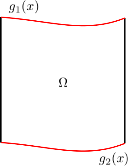
Figure 1: Curved boundary: domain $\Omega$ considered in such example, curved boundaries are highlighted in red.

Meshes

Computational meshes are obtained starting from polygonal meshes defined on the unit square $(0,1)^{2}$ and subsequently modified, following the idea proposed in [6]. In the present case, only the $y$-component of a generic point $P$ is modified, i.e., the point $P(x_{P},\,y_{P})$ becomes $P^{\prime}(x_{P}^{\prime},\,y_{P}^{\prime})$ where

$${x_{P}^{\prime}=x_{P}\qquad\text{and}\qquad y_{P}^{\prime}=\begin{cases}y_{P}+g_{2}(x_{P})(1-2y_{P})&\text{if}\>y_{P}\leq 0.5\\[5.0pt] 1-y_{P}+g_{1}(x_{P})\,(2y_{P}-1)&\text{if}\>y_{P}>0.5\end{cases}\,.}$$

The curved part of the boundary is further exactly reproduced for the withGeo case. As initial meshes we consider the following types of discretization of the unit square: i) quad, a uniform mesh composed by squares; ii) hexR, a mesh composed by hexagons; iii) hexD, a mesh composed by distorted hexagons; iv) voro, a centroidal Voronoi tessellation. The last two types of meshes have some interesting features which challenge the robustness of the virtual element approach: in particular hexD meshes have distorted elements, whereas voro meshes have tiny edges, see Figure 2.

quad	hexR	hexD	voro

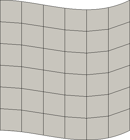
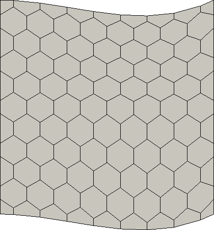
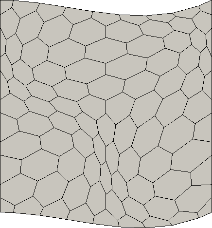
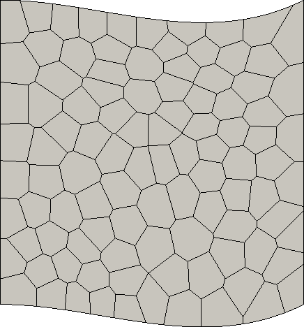
Figure 2: Curved boundary: types of discretization used to proceed with the convergence analysis.

Results

In Figures 3, 4, 5 and 6, we collect the results for the various types of meshes. The reported convergence lines of the withGeo and noGeo approaches coincide for polynomial degrees $k=0$ and 1. They have the expected convergence rate of $O\left(h^{1}\right)$ and $O\left(h^{2}\right)$, respectively. On the contrary, for polynomial degree $k>1$ the trend of both velocity and pressure $L^{2}$ errors is different between the two strategies.

More specifically, the convergence trends of the noGeo case is bounded by the geometrical representation error to $O\left(h^{2}\right)$, as this error dominates the accuracy of the approximation with mixed virtual elements. On the contrary the proposed approximation scheme withGeo behaves as expected for both velocity and pressure variables and for each approximation degree, showing the optimal convergence trend for the used polynomial degree. Such behaviour is in line to what observed in [6] for a Laplace problem.

quad

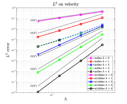
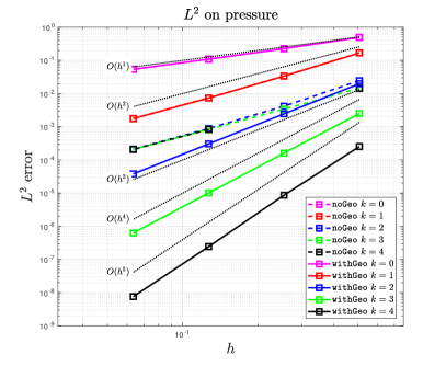
Figure 3: Curved boundary: convergence lines for quad meshes for each VEM approximation degrees.

hexR

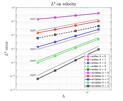
Figure 4: Curved boundary: convergence lines for hexR meshes for each VEM approximation degrees.

hexD

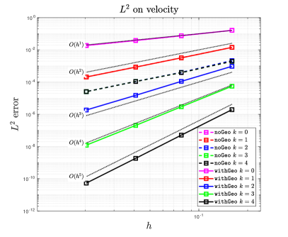
Figure 5: Curved boundary: convergence lines for hexD meshes for each VEM approximation degrees.

voro

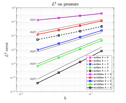
Figure 6: Curved boundary: convergence lines for voro meshes for each VEM approximation degrees.

5.2 Internal curved interface

Problem description

In this subsection we consider again Problem 1 defined on a different domain with respect to the previous example. The domain $\Omega$ is shown in Figure 7a and consists of a unit square $\Omega=(-1,\,1)^{2}$, $\Omega=\overline{\Omega_{1}}\cup\overline{\Omega_{2}}$, being $\Omega_{2}$ a circular inclusion with radius $R=0.45$ and $\Omega_{1}:=\Omega\backslash\Omega_{2}$ a circular crown. Two different values of the tensor $\kappa=k\mathbb{I}$ are prescribed on each subdomain: $k_{1}=1$ and $k_{2}=0.1$ for the subdomain $\Omega_{1}$ and $\Omega_{2}$, respectively, while $\mu=1.$ on each subdomain. We set the right hand side and the boundary conditions in such a way that the exact solution for the pressure is

$$p_{1}(x,\,y)=k_{2}\cos\left(\sqrt{x^{2}+y^{2}}\right)+\cos(R)\,(1-k_{2})$$

and

$$p_{2}(x,\,y)=\cos\left(\sqrt{x^{2}+y^{2}}\right)\,,$$

for the subdomains $\Omega_{1}$ and $\Omega_{2}$, respectively. Then, the exact solution for the velocity variable is given by

$$\bm{q}_{i}(x,\,y)=-k_{i}(x,\,y)\nabla p_{i}(x,\,y)\,,\qquad\text{for }i=1,2\,.$$

The pressure solution is chosen in such a way that we have a $C^{0}$ continuity on $\partial\Omega_{2}$, and the velocity field has a $C^{0}$ continuity of the normal component across $\partial\Omega_{2}$, i.e.,

$$p_{1}=p_{2}\qquad\text{and}\qquad\bm{q}_{1}\cdot\bm{n}_{\iota}+\bm{q}_{2}\cdot\bm{n}_{\iota}=0\qquad\text{on}\,\,\partial\Omega_{2}\,,$$

where $\bm{n}_{\iota}$ is the normal of $\partial\Omega_{2}$ pointing from $\Omega_{1}$ to $\Omega_{2}$.

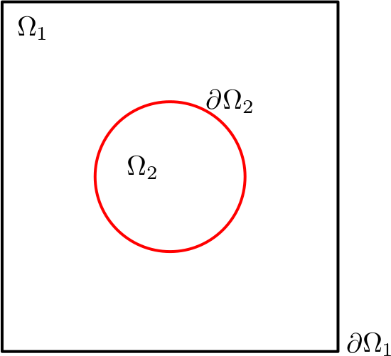
(a) Domain

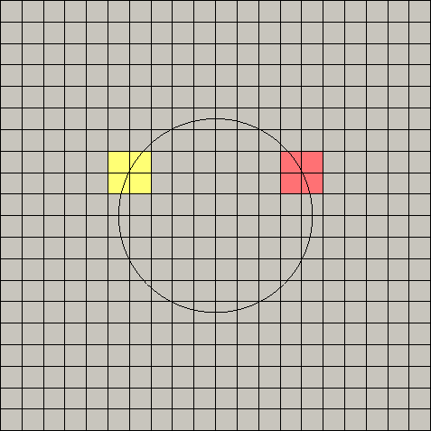
(b) Mesh

Figure 7: Internal curved interface. On the left, domain $\Omega$ considered in such example, curved boundaries are highlighted in red. On the right, the whole mesh with the internal curved boundary. We show zooms of the yellow and red regions in Figure 8.

Meshes

To generate the grid, we start again from a structured mesh composed of square elements of the whole domain $\Omega$, independently of the internal interface $\partial\Omega_{2}$, and then we cut the mesh elements into sub-elements according to $\partial\Omega_{2}$. The geometry of the internal interface is exactly reproduced in the proposed withGeo approach, whereas it is replaced by straight edges in the noGeo approach. In both cases, thanks to the ability of virtual elements in dealing with arbitrary shaped elements the mesh generation process is straightforward, as we do not need to re-mesh elements crossed by the circle, but we simply cut each intersected quadrilateral element into two new elements with one new (curved) edge, without taking care about the resulting shape and size of the two cut elements.

The flexibility in including interfaces in the mesh and the robustness with respect to element size/distortion are a huge advantage from the mesh generation point of view. In many applications a large number of possibly intersecting interfaces might be present in the computational domain, such that a robust and easy mesh generation process is of paramount importance. In such cases, the generation of good quality triangular meshes constrained to the interfaces might be an extremely complex task which might result in overly refined regions of the mesh, only needed to honour the geometry of the interfaces, independently from the desired accuracy level. If we consider a virtual element approach, interfaces can be easily superimposed to an existing regular mesh, as shown above, avoid unnecessary refinements and consequently decreasing the degrees of freedom and the computational effort.

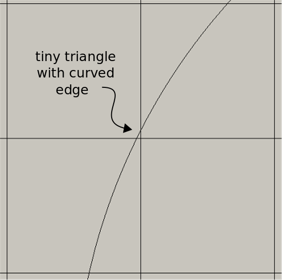
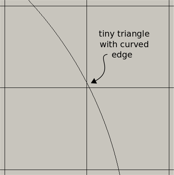
Figure 8: Internal curved interface: zooms of the yellow and red regions of Figure 7b, where we highlight tiny triangles with a curved edge.

In Figure 8 we show a detail of some cut elements. Here we better appreciate that elements crossed by the interface are simply split in two parts and there is no any further subdivision. Moreover, we notice that such meshing procedure might results in really tiny elements adjacent to big ones. In each mesh of the following convergence analysis there are many elements with these characteristics and we will see that the convergence trend of the method is not affected by them.

As a final remark, we would like to underline another interesting property of the proposed approach. The proposed curved spaces are compatible with standard finite element discretizations. For instance it is possible to simply glue a standard Raviart-Thomas element with an element with curved edges along a straight edges, thus exploiting the proposed virtual element spaces only on the elements with curvilinear edges and standard Raviart-Thomas discretization on elements with straight edges.

As we have done for the previous example we make a sequence of four meshes with decreasing mesh size $h$ to proceed with the convergence analysis.

Results

In Figure 9 we show the convergence lines for the withGeo and noGeo approaches as $h$ is reduced, for values of $k$ ranging between $0$ and $4$. The behaviour of the error is similar to the one shown in the previous example. Indeed, in the noGeo case the convergence is the optimal one for polynomial accuracy values $k=0$ and $1$, while for $k>1$ the geometrical error dominates the VEM approximation error and the trend remains bounded by $O\left(h^{2}\right)$. On the contrary, when we consider the virtual element spaces for curvilinear edges, optimal error decay $O\left(h^{k+1}\right)$ is obtained for both velocity and pressure $L^{2}$ errors, for the used polynomial accuracy $k$. A pre-asymptotic behaviour is observed for the withGeo approach for values of $k=2,3$ and 4, which however terminates in the considered range of $h$ values for almost all cases.

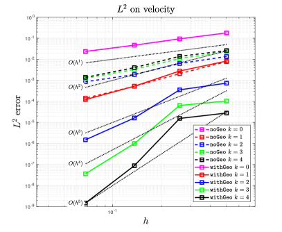
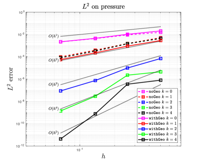
Figure 9: Internal curved interface: convergence lines for each VEM approximation degrees.

5.3 Double internal curved interfaces

Problem description

In this example we consider two internal boundaries which identify three regions, $\Omega_{1}$, $\Omega_{2}$ and $\Omega_{3}$, inside the square $(-1,\,1)^{2}$, see Figure 10a. Both internal boundaries are curved, i.e., $\Gamma_{1}$ and $\Gamma_{2}$ are defined as

$$g_{1}(x)=a\sin(\pi x)+b\qquad\text{and}\qquad g_{2}(x)=a\sin(\pi x)-b\,,$$

respectively. For this example we set $a=0.2$ and $b=0.31$. Then, we set the right hand side of Problem 1 in such a way that the pressure solution is

$$p_{1}(x,\,y) = a\sin(\pi x)\,,$$

$$p_{2}(x,\,y) = a\,\sin\left\{\frac{\pi}{2b}[y-a\sin(\pi x)]\right\}\sin(\pi\,x)\,,$$

$$p_{3}(x,\,y) = -a\sin(\pi x)\,,$$

and the velocity $\bm{q}_{i}(x,\,y)=-\nabla p_{i}(x,\,y)$ on each subdomain $\Omega_{i}$ for $i=1,2$ and $3$. Both velocity and pressure functions are chosen in such a way that we have a $C^{0}$ continuity for the pressure and for the normal component of the velocity on the curves $\Gamma_{1}$ and $\Gamma_{2}$, i.e.,

$$p_{1}=p_{2}\quad\text{and}\quad\bm{q}_{1}\cdot\bm{n}_{1}+\bm{q}_{2}\cdot\bm{n}_{1}=0\qquad\text{on}\,\,\Gamma_{1}\,,$$

$$p_{2}=p_{3}\quad\text{and}\quad\bm{q}_{2}\cdot\bm{n}_{2}+\bm{q}_{3}\cdot\bm{n}_{2}=0\qquad\text{on}\,\,\Gamma_{2}\,,$$

where $\bm{n}_{1}$ is the normal of $\Gamma_{1}$ pointing from $\Omega_{1}$ to $\Omega_{2}$ and $\bm{n}_{2}$ is the normal of $\Gamma_{2}$ pointing from $\Omega_{2}$ to $\Omega_{3}$.

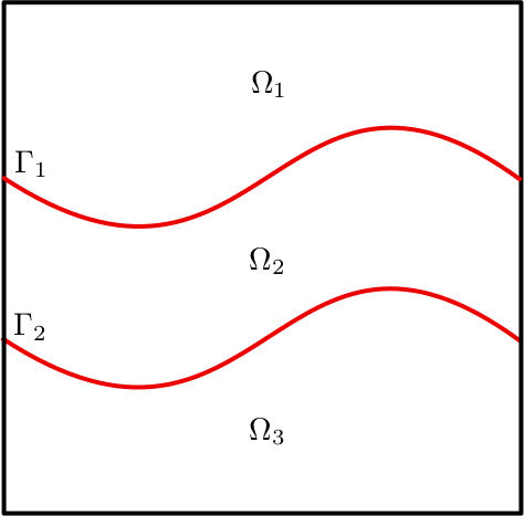
(a) Domain

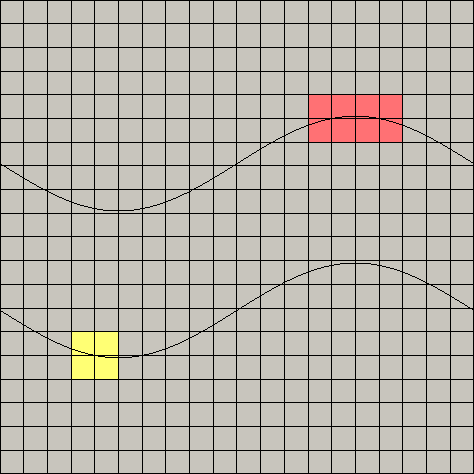
(b) Mesh

Figure 10: Double internal curved interfaces. On the left, domain $\Omega$ considered in such example, curved boundaries are highlighted in red. On the right, the whole mesh with the internal curved boundaries. We show zooms of the yellow and red regions in Figure 11.

Meshes

To generate the meshes, we follow the same idea as the example of Subsection 5.2. We build a background mesh composed by squares and then we insert the curved internal interfaces, as shown in Figure 10b. This is done, as previously, independently from the background mesh, and thus the resulting meshes are composed by elements with arbitrary size and shape, see Figure 11. Also in this case, mesh element edges lying on the curvilinear interfaces exactly match the interface for the withGeo approach, whereas they are approximated by straight edges in the noGeo case.

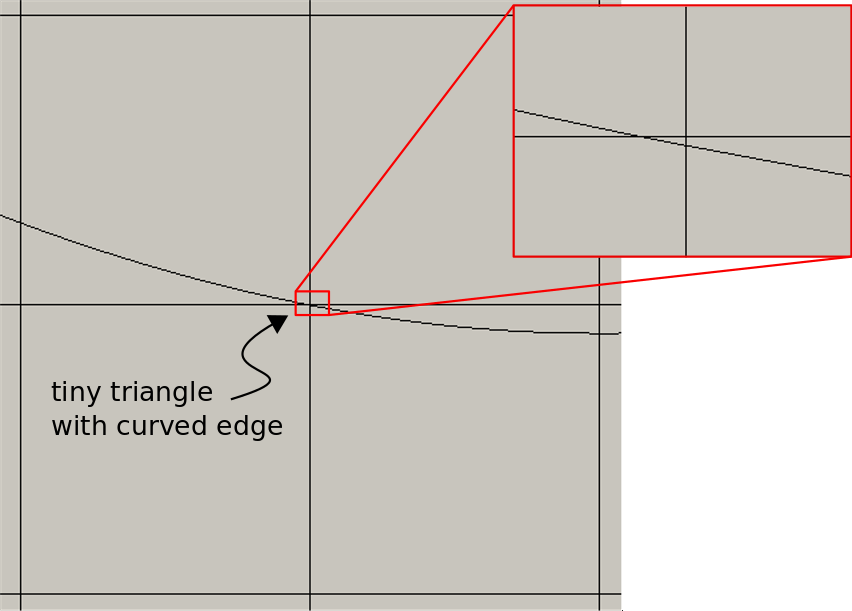
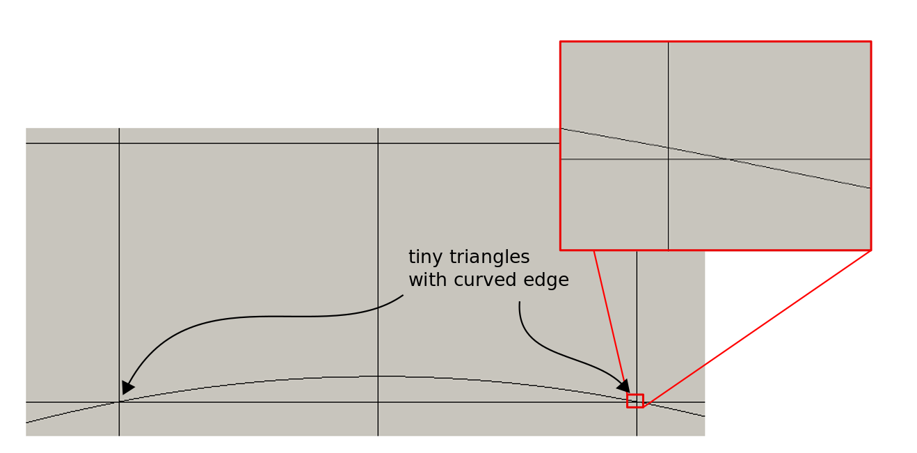
Figure 11: Double internal curved interfaces: zooms of the yellow and red regions of Figure 10b, where we highlight tiny triangles with a curved edge.

Results

In Figure 12 we show convergence lines for both the withGeo and noGeo for values of $k=0,\ldots,4$. The behaviour of error decay is again as expected: in the noGeo case error decay follows the expected trend for the used polynomial accuracy only for $k\leq 1$, being, for $k>1$, always $O\left(h^{2}\right)$ for the prevailing effect of the geometrical error. On the contrary, since appropriate basis functions are included in the definition of the approximation space in the proposed withGeo approach, optimal error decay is observed for the used polynomial accuracy level.

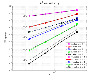
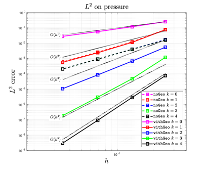
Figure 12: Double internal curved interfaces: convergence lines for each VEM approximation degrees.

6 Conclusions

In this work we have performed a first analysis on the extension of the mixed virtual element method to grids where elements might have curved edges, for elliptic problems in 2D. A theoretical analysis is proposed to show well-posedness of the discrete problem. A choice for the degrees of freedom particularly well suited for discretizations on curvilinear edge elements is highlighted, and a numerical scheme is proposed that handles in a coherent and consistent way the geometry, thus exhibiting optimal error decay in accordance to the polynomial accuracy level of the approximation. This is particularly suited for real applications where the geometrical error might dominate and limit the accuracy of the numerical solution. The numerical examples are in accordance with the theoretical findings and showed the optimal error decay for a domain with curved boundary and a domain with internal interfaces in contrast with the standard mixed virtual element method where the geometrical error jeopardizes the performances. Natural extension of the current work are the introduction of the mixed virtual element method for three-dimensional problems with curved faces and for more general problems.

References

- [1] R. A. Adams. Sobolev spaces, volume 65 of Pure and Applied Mathematics. Academic Press, New York-London, 1975.
- [2] Douglas N. Arnold, Daniele Boffi, and Richard S. Falk. Quadrilateral finite elements. SIAM J. Numer. Anal., 42(6):2429–2451 (electronic), 2005.
- [3] Yuri Bazilevs, Lourenço Beirão da Veiga, John Austin Cottrell, Thomas Joseph Robert Hughes Hughes, and Giancarlo Sangalli. Isogeometric analysis: approximation, stability and error estimates for -refined meshes. Mathematical Models and Methods in Applied Sciences, 16(07):1031–1090, 2006.
- [4] Lourenço Beirão da Veiga, Franco Brezzi, Luisa Donatella Marini, and Alessandro Russo. H(div) and H(curl)-conforming VEM. Numerische Mathematik, 133(2):303–332, Jun 2014.
- [5] Lourenço Beirão da Veiga, Franco Brezzi, Luisa Donatella Marini, and Alessandro Russo. Mixed virtual element methods for general second order elliptic problems on polygonal meshes. ESAIM: M2AN, 50(3):727–747, 2016.
- [6] Lourenço Beirão da Veiga, Alessandro Russo, and Giuseppe Vacca. The virtual element method with curved edges. ESAIM: M2AN, 53(2):375–404, 2019.
- [7] L. Beirão da Veiga, F. Brezzi, L. D. Marini, and A. Russo. Virtual elements and curved edges. arXiv:1910.10184, 2019.
- [8] L. Beirão da Veiga, A. Pichler, and G. Vacca. A virtual element method for the miscible displacement of incompressible fluids in porous media. arXiv:1907.13080, 2019.
- [9] Matías Fernando Benedetto, Stefano Berrone, Andrea Borio, Sandra Pieraccini, and Stefano Scialò. A hybrid mortar virtual element method for discrete fracture network simulations. Journal of Computational Physics, 306:148 – 166, 2016.
- [10] Matías Fernando Benedetto, Andrea Borio, and Stefano Scialò. Mixed virtual elements for discrete fracture network simulations. Finite Elements in Analysis and Design, 134:55–67, 2017.
- [11] Silvia Bertoluzza, Micol Pennacchio, and Daniele Prada. High order VEM on curved domains. Rendiconti Lincei - Matematica e Applicazioni, 30(2):391–412, June 2019.
- [12] Daniele Boffi, Franco Brezzi, and Michel Fortin. Mixed Finite Element Methods and Applications. Springer Series in Computational Mathematics. Springer Berlin Heidelberg, 2013.
- [13] L. Botti and D. Di Pietro. Assessment of Hybrid High-Order methods on curved meshes and comparison with discontinuous Galerkin methods. J. Comput. Phys., 370:58–84, 2018.
- [14] S. C. Brenner and L. R. Scott. The Mathematical Theory of Finite Element Methods, volume 15 of Texts in Applied Mathematics. Springer, New York, third edition, 2008.
- [15] F. Brezzi, K. Lipnikov, and M. Shashkov. Convergence of mimetic finite difference method for diffusion problems on polyhedral meshes with curved faces. Math. Models Methods Appl. Sci., 16(2):275–297, 2006.
- [16] Franco Brezzi, Jim Douglas, Ricardo Durán, and Michel Fortin. Mixed finite elements for second order elliptic problems in three variables. Numerische Mathematik, 51(2):237–250, Mar 1987.
- [17] Franco Brezzi, Jim Douglas, and Donatella Luisa Marini. Two families of mixed finite elements for second order elliptic problems. Numerische Mathematik, 47(2):217–235, 1985.
- [18] Franco Brezzi, Richard S. Falk, and Donatella Luisa Marini. Basic principles of mixed virtual element methods. ESAIM: M2AN, 48(4):1227–1240, 2014.
- [19] Philippe G. Ciarlet and Pierre-Arnaud Raviart. Interpolation theory over curved elements, with applications to finite element methods. Computer Methods in Applied Mechanics and Engineering, 1(2):217–249, 1972.
- [20] F. Dassi, J. Gedicke, and L. Mascotto. Adaptive virtual elements with equilibrated fluxes. arXiv:2004.11220, 2020.
- [21] Fanco Dassi and Giuseppe Vacca. Bricks for the mixed high-order virtual element method: Projectors and differential operators. Applied Numerical Mathematics, 2019.
- [22] R. G. Durán and A. L. Lombardi. Error estimates for the Raviart–Thomas interpolation under the maximum angle condition. SIAM J. Numer. Anal., 46(3):1442–1453, 2008.
- [23] Alessio Fumagalli. Dual virtual element method in presence of an inclusion. Applied Mathematics Letters, 86:22–29, Dec. 2018.
- [24] Alessio Fumagalli and Eirik Keilegavlen. Dual virtual element method for discrete fractures networks. SIAM Journal on Scientific Computing, 40(1):B228–B258, 2018.
- [25] Alessio Fumagalli and Eirik Keilegavlen. Dual virtual element methods for discrete fracture matrix models. Oil & Gas Science and Technology - Revue d’IFP Energies nouvelles, 74(41):1–17, 2019.
- [26] Alessio Fumagalli, Anna Scotti, and Luca Formaggia. Performances of the mixed virtual element method on complex grids for underground flow. Accepted in SEMA SIMAI Springer Series. Available at arXiv:2002.11974 [math.NA], 2020.
- [27] Thomas Joseph Robert Hughes Hughes, John Austin Cottrell, and Yuri Bazilevs. Isogeometric analysis: CAD, finite elements, NURBS, exact geometry and mesh refinement. Computer Methods in Applied Mechanics and Engineering, 194(39):4135 – 4195, 2005.
- [28] Marc Lenoir. Optimal isoparametric finite elements and error estimates for domains involving curved boundaries. SIAM Journal on Numerical Analysis, 23(3):562–580, 1986.
- [29] P. Monk. Finite element methods for Maxwell’s equations. Oxford University Press, 2003.
- [30] Monica Montardini, Giancarlo Sangalli, and Lorenzo Tamellini. Optimal-order isogeometric collocation at galerkin superconvergent points. Computer Methods in Applied Mechanics and Engineering, 316:741 – 757, 2017. Special Issue on Isogeometric Analysis: Progress and Challenges.
- [31] Jean-Claude Nédélec. A new family of mixed finite elements in . Numerische Mathematik, 50(1):57–81, Jan 1986.
- [32] Pierre-Arnaud Raviart and Jean-Marie Thomas. A mixed finite element method for second order elliptic problems. Lecture Notes in Mathematics, 606:292–315, 1977.
- [33] Jean E. Roberts and Jean-Marie Thomas. Mixed and hybrid methods. In Handbook of numerical analysis, Vol. II, Handb. Numer. Anal., II, pages 523–639. North-Holland, Amsterdam, 1991.
- [34] Milos Zlamal. Curved elements in the finite element method. i. SIAM Journal on Numerical Analysis, 10(1):229–240, 1973.