Three-body bound states of an atom in a Fermi mixture

Abstract

We determine the three-body bound states of an atom in a Fermi mixture. Compared to the Efimov spectrum of three atoms in vacuum, we show that the Fermi seas deform the Efimov spectrum systematically. We demonstrate that this effect is more pronounced near unitarity, for which we give an analytical estimate. We show that in the presence of Fermi seas, the three-body bound states obey a generalized discrete scaling law. For an experimental confirmation of our prediction, we propose three signatures of three-body bound states of an ultracold Fermi mixture of Yb isotopes, and provide an estimate for the onset of the bound state and the binding energy.

I introduction

In a seminal paper, Ref. Efimov_1 , Efimov showed that three bosons that interact attractively in vacuum via short-range interactions form three-body bound states at interaction strengths that are not yet sufficient to support two-body bound states. He also showed that the number of the three-body bound states is in principle infinite, and that there is a geometric scaling law that governs the bound states Efimov_2 ; Braaten_universality ; Grimm_and_Ferlaino ; Pascal_review_paper ; Greene_review ; DIncao_review . Technical advances in the trapping and cooling of atoms trapping_atoms ; kF_and_n as well as in the Feshbach resonances many_body_ultracold_atoms ; Feshbach_resonance_Review have led to the observation of the Efimov effect in ultracold atomic gases Efimov_1st_expt ; expt_Li_K ; expt_ultracold_second_trimer ; expt_Li_Cs_1 ; expt_Li_Cs_2 ; Efimov_ultracold_summary and helium beams experiments expt_helium_beam_1 ; expt_helium_beam_2 . Excited three-body bound states were observed expt_ultracold_second_trimer ; expt_Efimov_scaling_factor , and the Efimov scaling law was confirmed. The Efimov effect was also generalized to more than three particles Pascal_review_paper ; four_body_0 . It was shown that for a critical mass ratio three fermions and a lighter particle form a four-body bound state four_body_1 . The four-body bound states of two heavy and two light bosons for different mass ratios was investigated in Ref. four_body_2 . The formation of a five-body bound state in fermionic mixtures was discussed in Ref. five_body_1 .

Recently, we demonstrated the formation of three-electron bound states in conventional superconductors, and showed that the trimer state competes with the formation of the two-electron Cooper pair Sanayei . For that, we modeled the interaction between two particles “$i$” and “$j$” as a negative constant $g_{ij}$ in momentum space for an incoming and outgoing momentum of a particle smaller than a cutoff $\Lambda_{i}$, following the reasoning of the Cooper problem Cooper . We fixed the cutoffs by a typical value of the Debye energy in a conventional superconductor Sanayei . In this paper we determine the three-body bound states of an atom in a Fermi mixture for contact interactions. To describe contact interactions we take the limit of the cutoffs $\Lambda_{i}$ to infinity. We show that this model is separable separable , leading to a system of two coupled integral equations. This model enables us to calculate the three-body bound-state spectrum in the presence of Fermi seas.

In this work, we consider a cold-atom system of Fermi mixtures. We assume a density of the species, labeled “2”, that interacts attractively with another species of the same density, labeled “3”. We assume that the two species “2” and “3” are in different internal states. Next, we include an additional atom, labeled “1”, that interacts attractively with the other atoms via contact interactions; see Fig. 1. In general, the three masses $m_{1}$, $m_{2}$, and $m_{3}$ can be different, but we are primarily interested in the case $m_{3}=m_{2}$. We assume that atom “1” is a fermion. A similar analysis can be applied when it is a boson. The species “2” and “3”define the Fermi seas with the Fermi momentum $k_{F}$. This imposes the constraints $k_{2}>k_{F}$ and $k_{3}>k_{F}$ on the momentum of atoms “2” and “3”, respectively. We also assume that the interatomic distances, proportional to $1/k_{F}$, are much larger than the range of the atomic interactions. With this, we neglect the many-body effects on the formation of a three-body bound state within the interatomic distances. For contact interactions we introduce the s-wave scattering lengths as it relates to the contact interaction in its regularized form. We also define a three-body parameter, $\Lambda$, in order to regularize the range of the three-body interactions and to prevent Thomas collapse Thomas_collapse . This parameter defines a length scale of the range of the atomic interactions using the van der Waals length Pascal_review_paper ; three_body_parameter_1 ; three_body_parameter_2 .

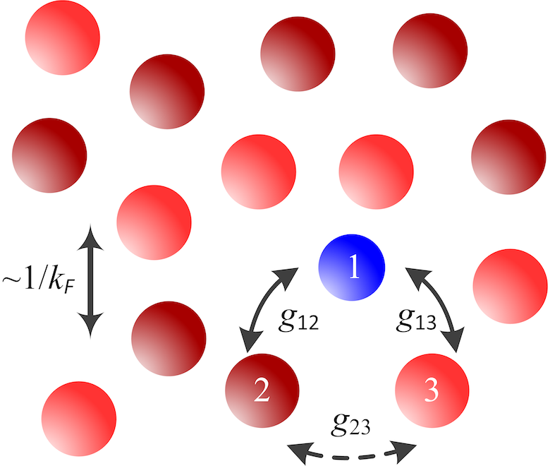
Figure 1: Sketch of an atom in a Fermi mixture. All species interact attractively via contact interactions. Species “2” and “3” are a Fermi mixture, and atom “1” can in general be a boson or fermion. The interaction strengths are shown by three negative constants $g_{12}$, $g_{13}$, and $g_{23}$. The species “2” and “3” are assumed to be in different internal states and $m_{3}=m_{2}$. The density of each species “2” and “3” is $n_{\mathrm{tot}}/2$, defining an inert Fermi sea with the Fermi momentum $k_{F}=(3\pi^{2}n_{\mathrm{tot}})^{1/3}$. The interatomic distances are proportional to $1/k_{F}$.

We calculate the three-body bound states for different mass ratios. We provide an analytical description of the lowest-energy two-body bound states and the two-body continuum, and find the three-body bound-state solutions numerically. For a noninteracting mixture, $g_{23}=0$, we provide an analytical formula for the onset of the lowest-energy two-body bound state at zero energy. For a high mass ratio $m_{2}/m_{1}$, where the excited three-body bound states appear, we also find an analytical estimate for the onset of a highest-energy excited three-body bound state at zero energy. With this, we can estimate the amount of the shift that the spectrum undergoes near unitarity due to the Fermi seas. Further, for our system and interaction model we demonstrate that a generalized scaling law governs the three-body bound states in the presence of Fermi seas. Finally, we propose three experimental scenarios in an ultracold system of fermionic mixtures of Yb isotopes to observe three-body bound states in the presence of Fermi seas. Here the ${}^{171}\mathrm{Yb}$ isotopes, that are in two different internal states, constitute the Fermi seas, and interact attractively with ${}^{173}\mathrm{Yb}$. We predict the onset of the three-body bound states and provide an estimate for the threshold energy.

This paper is organized as follows. In Sec. II we provide the main formulation of the problem for contact interactions, and derive a system of two coupled integral equations describing an atom in a Fermi mixture. In Sec. III we represent our results for two- and three interacting pairs in the presence of Fermi seas, and demonstrate a generalized scaling law governing the three-body bound states. Here we also derive an analytical estimate to describe the effect of the Fermi seas near unitarity. In Sec. IV we present three experimental signatures of a three-body bound state in an ultracold Fermi mixture of Yb isotopes. Finally, in Sec. V we present our concluding remarks.

II formulation of the problem

The Schrödinger equation for a system of three atoms in momentum space is

$$\left(\frac{\hbar^{2}k_{1}^{2}}{2m_{1}}+\frac{\hbar^{2}k_{2}^{2}}{2m_{2}}+\frac{\hbar^{2}k_{3}^{2}}{2m_{3}}+\hat{U}_{12}+\hat{U}_{13}+\hat{U}_{23}-E\right)\psi=0,$$ (1)

where $\hbar$ is the reduced Planck’s constant, $m_{i}$ and $\mathbf{k}_{i}$ is the atom mass and momentum, respectively, $E$ is the energy, and $\psi=\psi(\mathbf{k}_{1},\mathbf{k}_{2},\mathbf{k}_{3})$ is the wave function. We consider the interaction $\hat{U}_{ij}$ between the atom “$i$” and “$j$”, $i,j=1,2,3$ and $i\neq j$, as

$$\hat{U}_{ij}\psi=g_{ij}\theta_{\Lambda_{i}}(\mathbf{k}_{i})\theta_{\Lambda_{j}}(\mathbf{k}_{j})\int\frac{d^{3}\mathbf{q}}{(2\pi)^{3}}\theta_{\Lambda_{i}}(\mathbf{k}_{i}-\mathbf{q})\theta_{\Lambda_{j}}(\mathbf{k}_{j}+\mathbf{q})\psi,$$ (2)

where $\mathbf{q}$ is the momentum transfer momentum_transfer and $g_{ij}<0$ is the interaction strength; see Ref. Sanayei . The resulting operators $\hat{U}_{ij}\psi$ are given in Appendix B. The cutoff function $\theta_{a,b}(\mathbf{k})$ for two real numbers $0\leqslant a<b$ is defined as

$$\theta_{a,b}(\mathbf{k})=\begin{cases}1&\text{for }a\leqslant|\mathbf{k}|\leqslant b,\\ 0&\text{otherwise},\end{cases}$$ (3)

and $\theta_{b}(\mathbf{k})\equiv\theta_{0,b}(\mathbf{k})$. Here we consider three-body bound states with vanishing total momentum. We also consider a singlet state for the species “2” and “3” in the following. The Fermi seas demand the constraints $k_{2}>k_{F}$ and $k_{3}>k_{F}$ on the momentum of the atoms “2” and “3”, respectively. The threshold energy of the bound states is

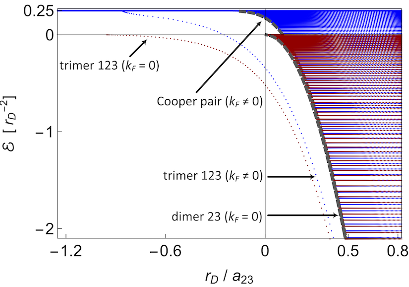
Figure 2: Energy $\mathcal{E}=2\mu_{12}E/\hbar^{2}$ in units of $r_{D}^{-2}$ vs $r_{D}/a_{23}$ for three interacting pairs, where $m_{2}/m_{1}=1$ and $a_{12}\approx-36r_{D}$. The red curves show the solution in vacuum, $k_{F}=0$. The blue curves show the result in the presence of Fermi seas, $k_{F}r_{D}\approx 0.17$. The single blue curve is the three-body bound-state solution for $k_{F}\neq 0$. The gray dashed curves are the lowest-energy two-body bound-state solutions of the two-body continuum in vacuum, cf. Eq. (A11), and in the presence of Fermi seas; cf. Eq. (15). The onset of the two-body bound-state continuum is shifted towards negative values of $a_{23}$. The onset of the three-body bound state is pushed towards positive values of $a_{23}$. The dependence of the trimer energy on $a_{23}$ is modified noticeably.

$$E_{\mathrm{thr}}=\frac{\hbar^{2}}{m_{2}}k_{F}^{2}=2E_{F},$$ (4)

where $E_{F}$ denotes the Fermi energy and $m_{3}=m_{2}$. To describe contact interactions we take the limit of the cutoffs $\Lambda_{i}$ and $\Lambda_{j}$ to infinity. We introduce the s-wave scattering length, $a_{ij}$, using the following regularization identity:

$$\frac{2\pi\hbar^{2}}{\mu_{ij}}\frac{1}{g_{ij}}+\frac{2}{\pi}\Lambda_{j}\equiv\frac{1}{a_{ij}}\text{ as }\Lambda_{j}\rightarrow\infty,$$ (5)

for $i,j=1,2,3$ and $i\neq j$; see Appendix A. Here, $\mu_{ij}$ is a reduced mass, $1/\mu_{ij}=1/m_{i}+1/m_{j}$, $m_{3}=m_{2}$, and $\Lambda_{i}\sim\Lambda_{j}$. Next, we define $\Lambda$ as the three-body parameter that fixes the range of the atomic interactions and regularizes the three-body bound states Pascal_review_paper ; three_body_parameter_1 ; three_body_parameter_2 . We also define a length scale, $r_{D}$, as

$$r_{D}=\frac{1}{\Lambda}.$$ (6)

The value of $\Lambda$ is chosen such that $\Lambda\gg k_{F}$, implying that $r_{D}\ll 1/k_{F}$. With this, we neglect the many-body effects on the formation of a three-body bound state. We determine $r_{D}$ as the range of the atomic interactions, which we take as the van der Waals length, $\ell_{ij}^{(\mathrm{vdW})}=\frac{1}{2}(2\mu_{ij}C_{6}/\hbar^{2})^{1/4}$, where $C_{6}$ is a dispersive coefficient associated with the polarizability of the electronic cloud of the atoms Pascal_review_paper ; Feshbach_resonance_Review ; C6_coeff_1 ; C6_coeff_Yb_1 ; C6_coeff_2 ; C6_coeff_3 . We also assume that the range of the interactions is much larger than the Compton wave length of the particles, $r_{D}\gg\lambda_{\mathrm{C}}$, implying that relativistic corrections to the three-body bound-state spectrum can be neglected. In what follows, we refer to a two-body bound state of atoms “$i$” and “$j$” as a dimer-$ij$, and to a three-body bound state of atoms “$i$”, “$j$” and “$l$” as a trimer-$ijl$. We also refer to a two-body bound state of species “2” and “3” as a Cooper pair for $k_{F}\neq 0$, and as a dimer-23 for $k_{F}=0$.

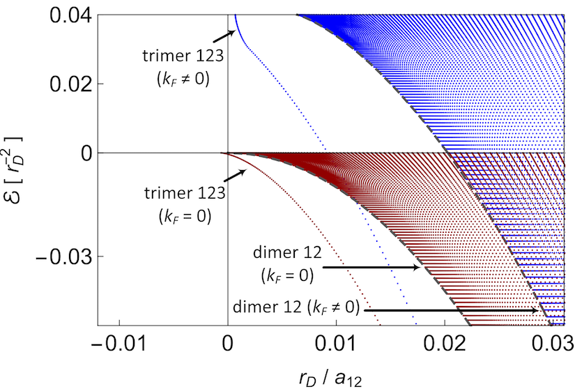
Figure 3: Energy $\mathcal{E}=2\mu_{12}E/\hbar^{2}$ in units of $r_{D}^{-2}$ vs $r_{D}/a_{12}$ for $g_{23}=0$ and $m_{2}/m_{1}=1$. The single red curve is the three-body bound-state solution for $k_{F}=0$, and the single blue curve is the solution for $k_{F}r_{D}\approx 0.02$. The gray dashed curves are the lowest-energy two-body bound states of the two-body continuum in vacuum, cf. Eq. (A11), and in the presence of Fermi seas; cf. Eq. (17). The Fermi seas push the onset of the two-body bound-state continuum as well as the onset of the three-body bound state to positive values of $a_{12}$.

 

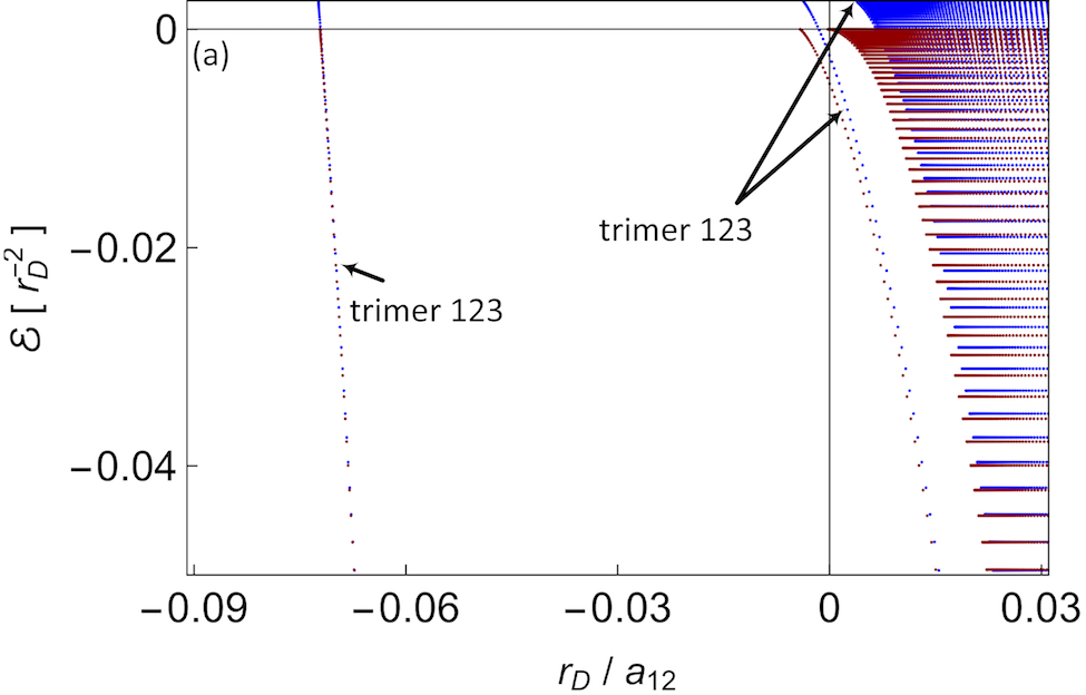
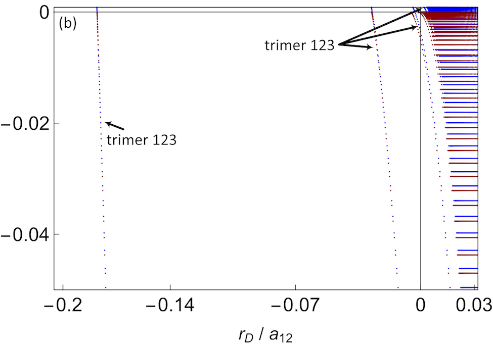
Figure 4: Energy $\mathcal{E}=2\mu_{12}E/\hbar^{2}$ in units of $r_{D}^{-2}$ vs $r_{D}/a_{12}$ for $g_{23}=0$. Red curves correspond to Efimov states, $k_{F}=0$, and blue curves are the results for $k_{F}r_{D}\approx 0.01$: (a) $m_{2}/m_{1}\approx 6.64$, (b) $m_{2}/m_{1}\approx 22.26$. As the mass ratio $m_{2}/m_{1}$ increases, excited three-body bound states appear. A zoom on the region where a highest-energy excited three-body bound state emerges is depicted in Fig. 5.

We note that the interaction model (2) is separable, as shown in Appendix B. This constitutes a system of the two coupled integral equations of the functions $F_{1}$ and $F_{2}$:

$$\Omega_{12}(g_{12},\mathbf{k}_{2};k_{F},E)F_{2}(\mathbf{k}_{2})= \xi_{1}(\mathbf{k}_{2};F_{2})+\xi_{2}(\mathbf{k}_{2};F_{1}),$$ (7)

$$\Omega_{23}(g_{23},\mathbf{k}_{1};k_{F},E)F_{1}(\mathbf{k}_{1})= \xi_{3}(\mathbf{k}_{1};F_{2}).$$ (8)

The two functions $\Omega_{12}$ and $\Omega_{23}$ describe the two-body bound state continuum, dimers-12 and dimers-23, respectively:

$$\Omega_{12}(g_{12},\mathbf{k}_{2};k_{F},E)=\frac{1}{g_{12}}+\int\frac{d^{3}\mathbf{p}_{3}}{(2\pi)^{3}}\,K_{1}(\mathbf{k}_{2},\mathbf{p}_{3};E),$$ (9)

$$\Omega_{23}(g_{23},\mathbf{k}_{1};k_{F},E)=\frac{1}{g_{23}}+\int\frac{d^{3}\mathbf{p}_{3}}{(2\pi)^{3}}\,K_{3}(\mathbf{k}_{1},\mathbf{p}_{3};E),$$ (10)

where for contact interactions we use the regularization relation (5) to introduce the s-wave scattering lengths. The three functions $\xi_{1}$, $\xi_{2}$, and $\xi_{3}$ describe the coupling of a pair to the third atom within the range of the length scale $r_{D}$ that is introduced by the three-body parameter $\Lambda$:

$$\xi_{1}(\mathbf{k}_{2};F_{2})=-\int\frac{d^{3}\tilde{\mathbf{p}}_{3}}{(2\pi)^{3}}\,\tilde{K}_{1}(\mathbf{k}_{2},\tilde{\mathbf{p}}_{3};E)F_{2}(\tilde{\mathbf{p}}_{3}),$$ (11)

$$\xi_{2}(\mathbf{k}_{2};F_{1})=-\int\frac{d^{3}\tilde{\mathbf{p}}_{1}}{(2\pi)^{3}}\,\tilde{K}_{2}(\mathbf{k}_{2},\tilde{\mathbf{p}}_{1};E)F_{1}(\tilde{\mathbf{p}}_{1}),$$ (12)

$$\xi_{3}(\mathbf{k}_{1};F_{2})=-2\int\frac{d^{3}\tilde{\mathbf{p}}_{3}}{(2\pi)^{3}}\,\tilde{K}_{3}(\mathbf{k}_{1},\tilde{\mathbf{p}}_{3};E)F_{2}(\tilde{\mathbf{p}}_{3});$$ (13)

see Appendix B. The integral kernels $K_{i}$ and $\tilde{K}_{i}$, $i=1,2,3$, and also the functions $F_{1}$ and $F_{2}$ are represented in Appendix B. We assume that $F_{i}(\mathbf{k})=F_{i}(k)$, implying s-wave symmetry of the states. We notice that the system of the integral Eqs. (7) and (8) can be interpreted as the Skorniakov–Ter-Martirosian equation for the zero-range limit of the interaction model (2); cf. Ref. Skorniakov_Ter-Martirosian .

III results

The coupled integral equations (7) and (8) describe three interacting pairs. For contact interactions and s-wave symmetry of the states we calculate the two functions $\Omega_{23}$ and $\Omega_{12}$ analytically; see Appendices C and D. These functions describe the lowest-energy two-body bound states and the two-body continuum, dimers-23 and dimers-12, respectively. Next, for a given value of the three-body parameter $\Lambda\gg k_{F}$ we evaluate the functions $\xi_{1}$, $\xi_{2}$, and $\xi_{3}$ numerically, and solve the system of the integral Eqs. (7) and (8) in order to find the three-body bound-state solutions. For that, we discretize the interval $(k_{F},\Lambda)$, and evaluate each integral as a truncated sum following the Gauss-Legendre quadrature rule Gaussian_quadrature_1 ; Gaussian_quadrature_2 ; Gaussian_quadrature_3 ; Gaussian_quadrature_4 . We construct the corresponding matrix equation and calculate the eigenvalues for different values of energy $E\leqslant E_{\mathrm{thr}}$, resulting in the s-wave scattering lengths $a_{23}$ and $a_{12}$. We find the values of the functions $F_{1}$ and $F_{2}$ at the grid points as the corresponding eigenvectors; see Appendix E. We note that the two-body bound states appear as continuum states, whereas the three-body bound states appear at discrete energy levels.

For three interacting pairs and for a fixed value of $a_{12}$, Fig. 2 shows the energy as a function of the inverse s-wave scattering length $1/a_{23}$ for $m_{2}/m_{1}=1$, and comparison with the result for $k_{F}=0$. It reveals a deformation of the Efimov spectrum in the presence of Fermi seas. We notice that for vanishing $k_{F}$, the two-body bound-state continuum emerges at unitarity, $a_{23}\rightarrow\pm\infty$, whereas the presence of Fermi seas expands the region of the two-body bound states to negative values of $a_{23}$. The single red and blue curves show the three-body bound-state solution for $k_{F}=0$ and $k_{F}\neq 0$, respectively. For $k_{F}\neq 0$ the three-body bound state emerges at a larger value of $|a_{23}|$ at $E=E_{\mathrm{thr}}$, and converges asymptotically to the three-body bound-state solution in vacuum. As a general tendency, the effect of the Fermi seas is more pronounced as we approach unitarity. Our results are consistent with Refs. Efimov_FermiSea_0_0 ; Efimov_FermiSea_0 ; Efimov_FermiSea_1 ; Efimov_FermiSea_2 ; QCD_Efimov_Cooper , which explore different, but related scenarios.

   

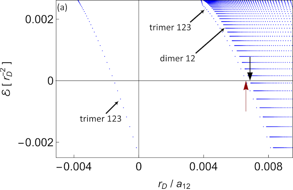
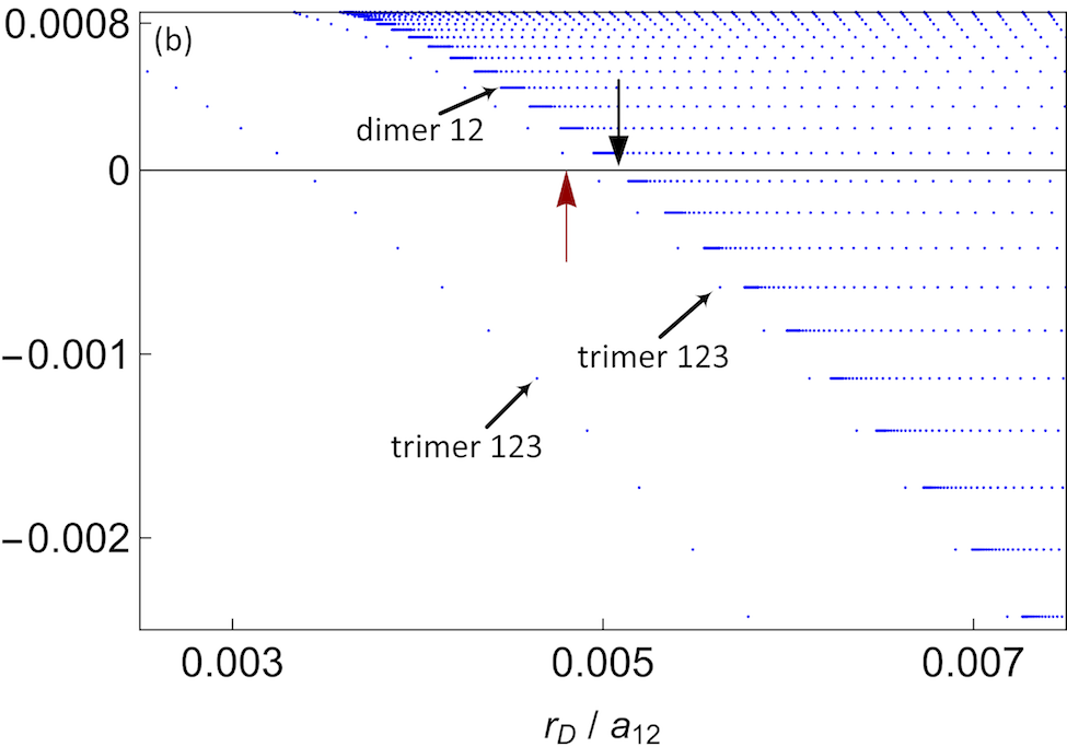
Figure 5: A zoom on the plot of energy $\mathcal{E}=2\mu_{12}E/\hbar^{2}$ in units of $r_{D}^{-2}$ vs $r_{D}/a_{12}$ for (a) $m_{2}/m_{1}\approx 6.64$ corresponding to Fig. 4(a), and (b) $m_{2}/m_{1}\approx 22.26$ corresponding to Fig. 4(b). Both panels show the region where a highest-energy excited three-body bound state emerges. The red vertical arrow locates the onset of a highest-energy excited three-body bound state at zero energy, given by Eq. (19). The black vertical arrow locates the onset of the lowest-energy two-body bound state at zero energy, given by Eq. (18).

To find an analytical solution of the lowest-energy two-body bound state, Cooper pair-23, we note that for $g_{12},g_{13}=0$ the system of the integral Eqs. (7) and (8) reduces to

$$\frac{1}{g_{23}}+\lim_{\Lambda_{2}\rightarrow\infty}\int\frac{d^{3}\mathbf{p}_{3}}{(2\pi)^{3}}\,\frac{\theta_{k_{F},\Lambda_{2}}(\mathbf{p}_{3})}{\frac{\hbar^{2}}{m_{2}}p_{3}^{2}-E_{23}}=0,$$ (14)

where $E_{23}<0$ is the bound-state energy of the Cooper pair. We use the regularization relation (5) and solve Eq. (14) for s-wave symmetry of the states, resulting in

$$\frac{1}{a_{23}}= \frac{2}{\pi}k_{F}+\frac{2}{\pi}\sqrt{-\mathcal{E}_{23}}\arctan\left(\frac{\sqrt{-\mathcal{E}_{23}}}{k_{F}}\right),$$ (15)

where $\mathcal{E}_{23}=2\mu_{23}E_{23}/\hbar^{2}$ and $\mu_{23}$ is a reduced mass, $1/\mu_{23}=1/m_{2}+1/m_{3}=2/m_{2}$; see gray dashed curves in Fig. 2. Far from the resonance, the Cooper-pair solution for $k_{F}\neq 0$ converges asymptotically to the lowest-energy two-body bound state in vacuum, $1/a_{23}=\sqrt{-\mathcal{E}_{23}}$, described by Eq. (15) as $k_{F}\rightarrow 0$.

For a noninteracting mixture, $g_{23}=0$, Eq. (8) has no effect anymore. For s-wave symmetry of the states the integral Eq. (7) reduces to

$$\Omega_{12}F_{2}(k_{2})= -\frac{1}{2\pi\frac{\mu_{12}}{m_{1}}k_{2}}\int_{k_{F}}^{\Lambda}d\tilde{p}_{3}\,\tilde{p}_{3}$$

$$\times\ln\left(\frac{\tilde{p}_{3}^{2}+\frac{2\mu_{12}}{m_{1}}k_{2}\tilde{p}_{3}+k_{2}^{2}-\mathcal{E}}{\tilde{p}_{3}^{2}-\frac{2\mu_{12}}{m_{1}}k_{2}\tilde{p}_{3}+k_{2}^{2}-\mathcal{E}}\right)F_{2}(\tilde{p}_{3}),$$ (16)

where $\mathcal{E}=2\mu_{12}E/\hbar^{2}$, $E$ is the energy of the three-body bound state, and $\mu_{12}$ is a reduced mass, $1/\mu_{12}=1/m_{1}+1/m_{2}$; see Appendix D. The analytical calculation of the function $\Omega_{12}$ is given by Eq. (D4). We solve the integral Eq. (16) numerically, using the Gauss-Legendre quadrature rule; see Appendix E. Figure 3 shows the result for vanishing and nonvanishing $k_{F}$, where $m_{2}/m_{1}=1$. In the presence of the Fermi seas, the onset of the three-body bound state is pushed to positive values of $a_{12}$, and the three-body bound-state solution converges asymptotically to the corresponding Efimov state in vacuum.

Figure 6: Demonstration of the generalized scaling law (20) and (21) for $g_{23}=0$ and $m_{2}/m_{1}\approx 22.26$: (a) energy $\mathcal{E}=2\mu_{12}E/\hbar^{2}$ in units of $r_{D}^{-2}$ vs $r_{D}/a_{12}$ for $k_{F}r_{D}\approx 0.01$, (b) rescaled energy $\mathcal{\tilde{E}}=2\mu_{12}\tilde{E}/\hbar^{2}$ in units of $r_{D}^{-2}$ vs rescaled $r_{D}/\tilde{a}_{12}$, for $k_{i}\mapsto\lambda k_{i}$, $i=1,2,3$, $k_{F}\mapsto\lambda k_{F}$, $a_{12}\mapsto\lambda^{-1}a_{12}$, $E\mapsto\lambda^{2}E$, where $\lambda=\exp(\pi/|s_{0}|)\approx 4.84998$. The red vertical arrow in panel (a) locates the onset of the ($n+1$)-th excited three-body bound state at $\mathcal{E}_{\mathrm{thr}}=2\mu_{12}E_{\mathrm{thr}}/\hbar^{2}$. The red vertical arrow in (b) locates the onset of the $n$-th excited three-body bound state of the rescaled spectrum at $\mathcal{\tilde{E}}_{\mathrm{thr}}=\lambda^{2}\mathcal{E}_{\mathrm{thr}}$. The gray dashed lines in both panels show the value of $\mathcal{E}_{\mathrm{thr}}$.

We note that for a given value of $k_{F}$, as we increase the mass ratio $m_{2}/m_{1}$, excited three-body bound states appear excited_trimers . Figure 4(a) shows the result for $m_{2}/m_{1}\approx 6.64$, where two excited additional three-body bound states are visible. In Fig. 4(b) we increase the mass ratio to $m_{2}/m_{1}\approx 22.26$, and obtain three excited three-body bound states. The red curves in Fig. 4(a) and Fig. 4(b) show the result in vacuum, which are the Efimov states. The blue curves show the result in the presence of Fermi seas. Near unitarity the Fermi seas have a noticeable influence on the spectrum. Far from the resonance and for low energies, the effect of the Fermi seas is negligible. In the presence of the Fermi seas the translational invariance is broken, and the Efimov scaling law in vacuum does not hold anymore, which we discuss in the following.

For $g_{23}=0$ we describe the two-body bound-state continuum, dimers-12, by solving

$$\Omega_{12}(a_{12},k_{2};k_{F},\mathcal{E}_{12})=0,$$ (17)

where $\Omega_{12}$ is given by Eq. (D4), $\mathcal{E}_{12}=2\mu_{12}E_{12}/\hbar^{2}$, and $E_{12}$ is the energy of the dimers-12. For the lowest-energy dimer-12 we solve Eq. (17) as $k_{2}\rightarrow k_{F}$. The result converges asymptotically to the lowest-energy two-body bound-state solution in vacuum; see gray dashed curves in Fig. 3 for $m_{2}/m_{1}=1$. At zero energy we find an analytical estimate for the onset of the the lowest-energy two-body bound state. For that, we solve Eq. (17) as $k_{2}\rightarrow k_{F}$ and $\mathcal{E}_{12}\rightarrow 0$, resulting in a critical s-wave scattering length, $a_{12,\mathrm{dimer}}^{(c)}\equiv a_{12}(E_{12}=0)$:

$$\frac{1}{a_{12,\mathrm{dimer}}^{(c)}}= \frac{k_{F}}{\pi}\left[1+\frac{1+\frac{2m_{2}}{m_{1}}}{\frac{2m_{2}}{m_{1}}(1+\frac{m_{2}}{m_{1}})}\ln\left(1+\frac{2m_{2}}{m_{1}}\right)\right.$$

$$\left.+\frac{\pi}{2}\frac{1}{1+\frac{m_{2}}{m_{1}}}\sqrt{1+\frac{2m_{2}}{m_{1}}}\right].$$ (18)

Equation (18) gives an estimate of the shift to the repulsive region of $a_{12}$ that the lowest-energy two-body bound state undergoes at zero energy in the presence of Fermi seas; see black vertical arrows in Fig. 5(a) and 5(b). For $m_{2}\gg m_{1}$ this amount approaches $k_{F}/\pi$.

Moreover, for $g_{23}=0$ and a high mass ratio $m_{2}/m_{1}\gg 1$, we find an analytical estimate for the onset of a highest-energy excited three-body bound state at zero energy. For that, we note that near the Fermi surface we can approximate the momentum of the species “2” and “3” to be around $k_{F}$ but in opposite directions, $\mathbf{k}_{2}\sim-\mathbf{k}_{3}$. Because we have assumed that the total momentum of the three-body bound state is zero, this results in the vanishing momentum of the atom “1”, $\mathbf{k}_{1}\sim\mathbf{0}$. Next, we consider the pair-12, where $m_{2}/m_{1}\gg 1$ and $k_{1}\sim 0$. With these assumption, the relative momentum of the pair-12, defined as $\mathbf{p}_{12}\equiv[m_{2}/(m_{1}+m_{2})]\mathbf{k}_{1}-[m_{1}/(m_{1}+m_{2})]\mathbf{k}_{2}$, approaches zero. We note that the Fermi surface, $k_{2}\sim k_{F}$, can be described in terms of the relative momentum, $\mathbf{p}_{12}$, and total momentum, $\mathbf{P}_{12}$, of the pair-12 as $|(\mu_{12}/m_{1})\mathbf{P}_{12}-\mathbf{p}_{12}|\sim k_{F}$, where $\mathbf{P}_{12}\equiv\mathbf{k}_{1}+\mathbf{k}_{2}$; see Appendix F. This implies that for $m_{2}/m_{1}\gg 1$ and $k_{1}\sim 0$ we can approximate the total momentum of the pair-12 to be $P_{12}\sim(\mu_{12}/m_{1})^{-1}k_{F}$. We also note that for large mass ratios $m_{2}/m_{1}$, the threshold energy of the three-body bound state, $\mathcal{E}_{\mathrm{thr}}=2\mu_{12}E_{\mathrm{thr}}/\hbar^{2}=2(1-\mu_{12}/m_{1})k_{F}^{2}$, approaches the threshold energy of the pair-12, $\mathcal{E}_{\mathrm{thr}}^{(12)}=\mathcal{E}_{\mathrm{thr}}/2$. To find the onset of a highest-energy excited three-body bound state at $E=0$, we calculate the onset of the lowest-energy pair-12 for total momentum $P_{12}\sim(\mu_{12}/m_{1})^{-1}k_{F}$ and $E_{12}\sim 0$. To do this, we use the interaction model (2), and write the Schrödinger equation describing the pair-12 for a contact interaction in terms of the relative and total momenta; see Appendix F. The solution for $P_{12}\rightarrow(\mu_{12}/m_{1})^{-1}k_{F}$ and $E_{12}\rightarrow 0$ results in an estimate for the critical s-wave scattering length, $a_{12,\mathrm{trimer}}^{(c)}\equiv a_{12}(E\approx 0)$:

$$\frac{1}{a_{12,\mathrm{trimer}}^{(c)}}\approx \frac{k_{F}}{\pi}\left[1+\frac{1}{4}\frac{1}{1+\frac{m_{2}}{m_{1}}}\ln\left(4(1+\frac{m_{2}}{m_{1}})\right)\right.$$

$$\left.-\frac{\pi}{2}\frac{1}{\sqrt{1+\frac{m_{2}}{m_{1}}}}+\frac{1}{2}\frac{1}{1+\frac{m_{2}}{m_{1}}}\right]\text{for }\frac{m_{2}}{m_{1}}\gg 1;$$ (19)

see Appendix F. For a high mass ratio $m_{2}/m_{1}\gg 1$, Eq. (19) gives an estimate for the amount of the shift to the repulsive region of $a_{12}$ that a highest-energy excited three-body bound state undergoes at zero energy in the presence of Fermi seas. Figure 5 reveals a zoom on the region where a highest-energy three-body bound state emerges for $m_{2}/m_{1}=6.64$ and $m_{2}/m_{1}\approx 22.26$. The red vertical arrows locate the critical value (19). For a very large mass ratio $m_{2}/m_{1}$, the critical value (19) eventually approaches $k_{F}/\pi$, converging to the lowest-energy two-body bound state at zero energy. Equations (18) and (19) provide a quantitative analysis for the effect of the Fermi seas on the near-resonant spectrum.

Finally, we elaborate on the observation that the Fermi seas deform the Efimov spectrum. This effect is more pronounced as we approach unitarity. As a result, the Efimov scaling factor that governs the three-body bound states in vacuum does not hold anymore. Here we show that a scaling transformation $k_{F}\mapsto\lambda k_{F}$, where $\lambda$ is the Efimov scaling factor, gives rise to a generalized scaling law for our system and interaction model (2). To this end, we notice that $k_{F}\mapsto\lambda k_{F}$ implies a scaling transformation of all momenta as $k_{i}\mapsto\lambda k_{i}$, for $i=1,2,3$. It also rescales the threshold energy as $E_{\mathrm{thr}}\mapsto\lambda^{2}E_{\mathrm{thr}}$, cf. Eq. (4), implying a general scaling transformation of energy as $E\mapsto\lambda^{2}E$. To ensure that the system of the coupled integral Eqs. (7) and (8) remains valid, it requires a scaling transformation of the s-wave scattering length as $a\mapsto\lambda^{-1}a$; see Eqs. (C6), (C9), and (D4). This results in a discrete scaling law for the three-body bound states in the presence of Fermi seas:

$$\frac{\lambda}{a_{n+1}(k_{F})}= \frac{1}{a_{n}(\lambda k_{F})},$$ (20)

$$\lambda^{2}E_{n+1}(k_{F},1/a)= E_{n}(\lambda k_{F},\lambda/a),$$ (21)

where $n\in\mathbb{N}$ is an index labeling the three-body bound state, $\lambda=\exp(\pi/|s_{0}|)$, and the parameter $s_{0}$, that depends on the mass ratio $m_{2}/m_{1}$, is determined in Appendix G. Our finding is in agreement with the result of Ref. Efimov_FermiSea_4 . Figure 6 demonstrates the generalized scaling law (20) and (21) for an atomic system of three fermions with a noninteracting mixture, $g_{23}=0$, and $m_{2}/m_{1}\approx 22.26$.

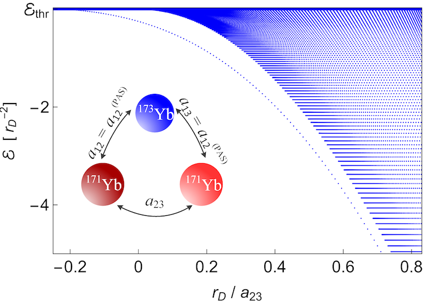
Figure 7: Visualization of the first scenario for the experimental signature of a three-body bound state in an ultracold fermionic mixture of Yb isotopes. The plot shows the energy $\mathcal{E}=2\mu^{(\mathrm{Yb})}E/\hbar^{2}$ in units of $r_{D}^{-2}$ vs $r_{D}/a_{23}$, where $r_{D}\equiv\ell_{23}^{(\mathrm{vdW})}\approx 4.145\text{ nm}$. The s-wave scattering length of ${}^{171}\mathrm{Yb}$ and ${}^{173}\mathrm{Yb}$ is fixed as the value measured via photoassociation spectroscopy (PAS), $a_{12}=a_{13}=a_{12}^{(\mathrm{PAS})}\approx-30.6\text{ nm}$. The three-body bound state emerges at $a_{23}\approx-20.7\text{ nm}$ at the threshold energy $E_{\mathrm{thr}}\approx 1.10\text{ kHz}$.

IV experimental signatures

We propose three scenarios to observe three-body bound states in mixtures of Yb isotopes, in particular a mixture of ${}^{171}\mathrm{Yb}$ and ${}^{173}\mathrm{Yb}$. In the terminology that is illustrated in Fig. 1, ${}^{173}\mathrm{Yb}$ plays the role of species “1”, and species “2” and “3” are two internal states of ${}^{171}\mathrm{Yb}$. The density of each of the ${}^{171}\mathrm{Yb}$ species is $n_{\mathrm{tot}}/2$, whereas the density of ${}^{173}\mathrm{Yb}$ is much smaller. We denote the s-wave scattering lengths of ${}^{171}\mathrm{Yb}$ and ${}^{173}\mathrm{Yb}$ by $a_{12}$ and $a_{13}$, and the s-wave scattering length of two ${}^{171}\mathrm{Yb}$ isotopes by $a_{23}$. We also assume that $a_{13}=a_{12}$.

As measured via two-color photoassociation spectroscopy (PAS), see Ref. C6_coeff_Yb_1 , ${}^{171}\mathrm{Yb}$ isotopes are almost noninteracting, while the s-wave scattering length between ${}^{171}\mathrm{Yb}$ and ${}^{173}\mathrm{Yb}$ atoms is $a_{12}^{(\mathrm{PAS})}\approx-30.6\text{ nm}\approx-578.23a_{0}$, where $a_{0}$ denotes the Bohr radius Bohr_radius . We note that ${}^{171}\mathrm{Yb}$ and ${}^{173}\mathrm{Yb}$ have almost the same atomic mass, where the reduced mass is $\mu_{12}\approx 85.9657\text{ u}$ NIST_data . The reduced mass of two ${}^{171}\mathrm{Yb}$ isotopes is $\mu_{23}\approx 85.4682\text{ u}$ NIST_data . The van der Waals dispersive coefficient, $C_{6}^{(\mathrm{Yb})}$, that determines the atomic interaction in a $\mathrm{Yb}_{2}$ molecule is given by Refs. C6_coeff_Yb_1 ; C6_coeff_Yb_2 . We calculate the van der Waals lengths to be $\ell_{12}^{(\mathrm{vdW})}=\frac{1}{2}[2\mu_{12}C_{6}^{(\mathrm{Yb})}/\hbar^{2}]^{1/4}\approx 4.151\text{ nm}\approx 78.44a_{0}$ and $\ell_{23}^{(\mathrm{vdW})}=\frac{1}{2}[2\mu_{23}C_{6}^{(\mathrm{Yb})}/\hbar^{2}]^{1/4}\approx 4.145\text{ nm}\approx 78.33a_{0}$. These values fix the corresponding length scales $r_{D}$. Next, for each internal state we assume that the density of ${}^{171}\mathrm{Yb}$ species is $n_{\mathrm{tot}}/2=\frac{1}{2}\times 10^{17}\text{ m}^{-3}$. We calculate the value of the Fermi momentum as $k_{F}=(3\pi^{2}n_{\mathrm{tot}})^{1/3}$; cf. Ref. kF_and_n .

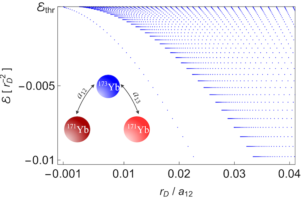
Figure 8: Visualization of the second scenario in which ${}^{171}\mathrm{Yb}$ and ${}^{173}\mathrm{Yb}$ are interact attractively, while the two ${}^{171}\mathrm{Yb}$ species are noninteracting. The plot shows the energy $\mathcal{E}=2\mu^{(\mathrm{Yb})}E/\hbar^{2}$ in units of $r_{D}^{-2}$ vs $r_{D}/a_{12}$, where $r_{D}\equiv\ell_{12}^{(\mathrm{vdW})}\approx 4.151\text{ nm}$ and $a_{13}=a_{12}$. The onset of the three-body bound state is at $a_{12}\approx-3193\text{ nm}$ with the threshold energy $E_{\mathrm{thr}}\approx 1.09\text{ kHz}$.

We adopt the s-wave scattering length of ${}^{171}\mathrm{Yb}$ and ${}^{173}\mathrm{Yb}$ as reported in Ref. C6_coeff_Yb_1 , i.e., $a_{12}=a_{12}^{(\mathrm{PAS})}$, and calculate the three-body bound-state solution for three interacting pairs Error . Figure 7 shows the three-body bound-state energy as a function of $1/a_{23}$. We find that the onset of the three-body bound state is $a_{23}\approx-20.7\text{ nm}\approx-391.16a_{0}$, emerging at the threshold energy $E_{\mathrm{thr}}\approx 1.10\text{ kHz}$. As a first experimental scenario, we propose to tune the interaction between two ${}^{171}\mathrm{Yb}$ isotopes via optical Feshbach resonances optical_Feshbach_1 ; optical_Feshbach_2 ; optical_Feshbach_3 ; optical_Feshbach_4 ; optical_Feshbach_5 , across the onset of the three-body bound state, which should result in increased atomic losses.

As a second scenario we consider two noninteracting ${}^{171}\mathrm{Yb}$ isotopes, and calculate the three-body bound-state solution for two interacting pairs ${}^{171}\mathrm{Yb}$ - ${}^{173}\mathrm{Yb}$. Figure 8 shows the energy of the three-body bound state as a function of $1/a_{12}$. It reveals that the three-body bound state emerges at $a_{12}\approx-3193\text{ nm}\approx-60336.40a_{0}$ at the threshold energy $E_{\mathrm{thr}}\approx 1.09\text{ kHz}$. Here the s-wave scattering length $a_{12}$ is much larger in amplitude than $a_{12}^{(\mathrm{PAS})}$, and the threshold energy is smaller than the value obtained in the first scenario. A three-body bound state is observed, if the interaction between two ${}^{171}\mathrm{Yb}$ and ${}^{173}\mathrm{Yb}$ is tuned via interisotope Feshbach resonances interisotope_Feshbach_1 , or via orbital Feshbach resonances orbital_Feshbach_2 ; orbital_Feshbach_3 .

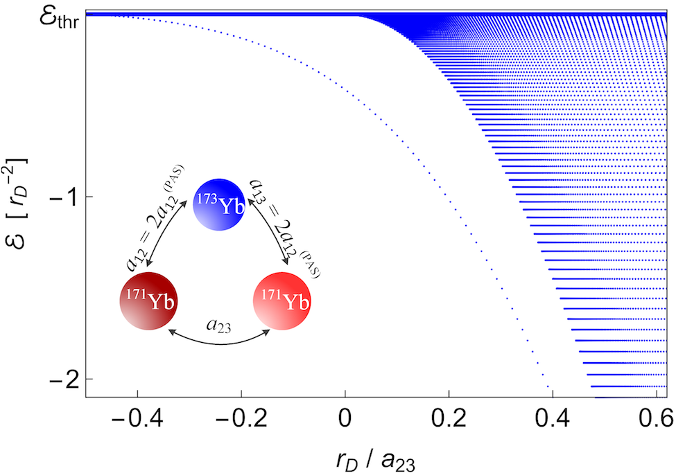
Figure 9: Visualization of the third scenario. The plot shows the energy $\mathcal{E}=2\mu^{(\mathrm{Yb})}E/\hbar^{2}$ in units of $r_{D}^{-2}$ vs $r_{D}/a_{23}$, where $r_{D}\equiv\ell_{23}^{(\mathrm{vdW})}\approx 4.145\text{ nm}$. The s-wave scattering length of ${}^{171}\mathrm{Yb}$ and ${}^{173}\mathrm{Yb}$ is fixed to be $a_{12}=a_{13}=2a_{12}^{(\mathrm{PAS})}\approx-2\times 30.6\text{ nm}$. The three-body bound state emerges at $a_{23}\approx-10.4\text{ nm}$ at the threshold energy $E_{\mathrm{thr}}\approx 1.10\text{ kHz}$.

As a third scenario, if the interaction between two ${}^{171}\mathrm{Yb}$ and ${}^{173}\mathrm{Yb}$ isotopes is tuned to a larger value in amplitude than $a_{12}^{(\mathrm{PAS})}$, e.g., $a_{12}=2a_{12}^{(\mathrm{PAS})}$, we find that the three-body bound state emerges at $a_{23}\approx-10.4\text{ nm}\approx-196.52a_{0}$ with the same threshold energy of the first scenario; see Fig. 9. Here the value of $a_{12}$ is much smaller in amplitude than the value obtained in the second scenario. Also, the value of $a_{23}$ is smaller in amplitude than the value found in the first scenario. A three-body bound state is observed, if the interaction between two ${}^{171}\mathrm{Yb}$ isotopes and also the interaction between ${}^{171}\mathrm{Yb}$ and ${}^{173}\mathrm{Yb}$ are tuned simultaneously.

We note that in all scenarios we have assumed that the interatomic distances are much larger than the range of the atomic interactions, $1/k_{F}\gg r_{D}$. The onset of the three-body bound states might slightly deviate if this criterion is not met. Here there will be a competition of ${}^{171}\mathrm{Yb}$ isotopes to form a three-body bound state with ${}^{173}\mathrm{Yb}$.

V conclusions

In conclusion, we have demonstrated and characterized three-body bound states of a single fermionic atom interacting with a Fermi mixture of two fermionic species. For this purpose, we have expanded and elaborated on a model previously used to determine trimer states in conventional superconductors, Ref. Sanayei . We have shown that the expanded interaction model is separable, leading to a system of integral equations in momentum space. Based on these equations we have presented their full numerical solution, as well as analytical solutions of limiting cases. Compared to three atoms interacting in vacuum, the presence of the Fermi seas renormalizes the eigenstates and eigenenergies, in particular near unitarity. Compared the Efimov scaling law of three atoms in vacuum, we have shown that our system and interaction model obeys a generalized discrete scaling law. We have also proposed three scenarios to obtain experimental signatures of the modified Efimov effect in an ultracold Fermi system of Yb isotopes.

ACKNOWLEDGMENTS

We acknowledge support from the Deutsche Forschungsgemeinschaft through Program No. SFB 925, and also The Hamburg Centre for Ultrafast Imaging. We would like to thank Pascal Naidon for very valuable discussions. A.S. also thanks C. Becker, K. Sponselee, B. Abeln, and L. Freystatzky for useful discussions on the experimental signatures of our results.

appendix a. introducing the s-wave scattering lengths

We consider the Schrödinger equation in momentum space governing two atoms “A” and “B” in vacuum:

$$\left(\frac{\hbar^{2}k_{\mathrm{A}}^{2}}{2m_{\mathrm{A}}}+\frac{\hbar^{2}k_{\mathrm{B}}^{2}}{2m_{\mathrm{B}}}+\hat{U}_{\mathrm{AB}}-E_{\mathrm{AB}}\right)\phi=0,$$ (A1)

where $m_{i}$ and $\mathbf{k}_{i}$, $i\in\{\mathrm{A},\mathrm{B}\}$, is the atom mass and momentum, respectively, $E_{\mathrm{AB}}$ is the energy, and $\phi=\phi(\mathbf{k}_{\mathrm{A}},\mathbf{k}_{\mathrm{B}})$ is the wave function. The interaction $\hat{U}_{\mathrm{AB}}$ between the atoms “A” and “B” follows from the interaction model (2). The resulting operator $\hat{U}_{\mathrm{AB}}\phi$ reads:

$$\hat{U}_{\mathrm{AB}}\phi= g_{\mathrm{AB}}\theta_{\Lambda_{\mathrm{A}}}(\mathbf{k}_{\mathrm{A}})\theta_{\Lambda_{\mathrm{B}}}(\mathbf{k}_{\mathrm{B}})\int\frac{d^{3}\mathbf{q}}{(2\pi)^{3}}\,\theta_{\Lambda_{\mathrm{A}}}(\mathbf{k}_{\mathrm{A}}-\mathbf{q})$$

$$\times\theta_{\Lambda_{\mathrm{B}}}(\mathbf{k}_{\mathrm{B}}+\mathbf{q})\phi(\mathbf{k}_{\mathrm{A}}-\mathbf{q},\mathbf{k}_{\mathrm{B}}+\mathbf{q}),$$ (A2)

where $g_{\mathrm{AB}}<0$ and $\mathbf{q}$ is the momentum transfer momentum_transfer . We assume the zero total momentum, $\mathbf{k}_{\mathrm{A}}+\mathbf{k}_{\mathrm{B}}=\mathbf{0}$, and $\Lambda_{\mathrm{B}}=\Lambda_{\mathrm{A}}$. Next, we define the variables $\bm{\kappa}_{i}\equiv\mathbf{q}+\mathbf{k}_{i}$, $i\in\{\mathrm{A},\mathrm{B}\}$, and write the Schrödinger Eq. (A1) as

$$\left(\frac{\hbar^{2}k_{\mathrm{A}}^{2}}{2\mu_{\mathrm{AB}}}-E_{\mathrm{AB}}\right)\phi(\mathbf{k}_{\mathrm{A}})= -g_{\mathrm{AB}}\theta_{\Lambda_{\mathrm{A}}}(\mathbf{k}_{\mathrm{A}})\int\frac{d^{3}\bm{\kappa}_{\mathrm{B}}}{(2\pi)^{3}}$$

$$\times\theta_{\Lambda_{\mathrm{A}}}(\bm{\kappa}_{\mathrm{B}})\phi(\bm{\kappa}_{\mathrm{B}}),$$ (A3)

where $\mu_{\mathrm{AB}}$ is a reduced mass, $1/\mu_{\mathrm{AB}}=1/m_{\mathrm{A}}+1/m_{\mathrm{B}}$. We define

$$\mathcal{F}\equiv-4\pi\left(\frac{2\mu_{\mathrm{AB}}}{4\pi\hbar^{2}}g_{\mathrm{AB}}\right)\theta_{\Lambda_{\mathrm{A}}}(\mathbf{k}_{\mathrm{A}})\int\frac{d^{3}\mathbf{k}_{\mathrm{A}}}{(2\pi)^{3}}\theta_{\Lambda_{\mathrm{A}}}(\mathbf{k}_{\mathrm{A}})\phi(\mathbf{k}_{\mathrm{A}}),$$ (A4)

and rewrite Eq. (A3) as

$$(k_{\mathrm{A}}^{2}-\mathcal{E}_{\mathrm{AB}})\phi(\mathbf{k}_{\mathrm{A}})=\mathcal{F},$$ (A5)

where $\mathcal{E}_{\mathrm{AB}}=2\mu_{\mathrm{AB}}E_{\mathrm{AB}}/\hbar^{2}$.

For $\mathcal{E}_{\mathrm{AB}}>0$ the solution of Eq. (A5) is

$$\phi(\mathbf{k}_{\mathrm{A}})=(2\pi)^{3}\delta^{(3)}(\mathbf{k}_{\mathrm{A}}-\mathbf{K})+\frac{\mathcal{F}}{k_{\mathrm{A}}^{2}-\mathcal{E}_{\mathrm{AB}}+i\varepsilon},$$ (A6)

where $0<\varepsilon\ll 1$, $|\mathbf{K}|^{2}=\mathcal{E}_{\mathrm{AB}}$, and $\delta^{(3)}$ denotes the three-dimensional Dirac delta function. We insert the ansazt (A6) into Eq. (A4):

$$\frac{\mathcal{F}}{4\pi\left(\frac{2\mu_{\mathrm{AB}}}{4\pi\hbar^{2}}g_{\mathrm{AB}}\right)}= -\theta_{\Lambda_{\mathrm{A}}}(\mathbf{k}_{\mathrm{A}})\int\frac{d^{3}\mathbf{k}_{\mathrm{A}}}{(2\pi)^{3}}\theta_{\Lambda_{\mathrm{A}}}(\mathbf{k}_{\mathrm{A}})\Bigl{[}(2\pi)^{3}$$

$$\times\delta^{(3)}(\mathbf{k}_{\mathrm{A}}-\mathbf{K})+\frac{\mathcal{F}}{k_{\mathrm{A}}^{2}-\mathcal{E}_{\mathrm{AB}}+i\varepsilon}\Bigr{]}.$$ (A7)

We note that in the zero-energy limit, $\mathcal{E}_{\mathrm{AB}}\rightarrow 0^{+}$, we have $\mathcal{F}=-4\pi a_{\mathrm{AB}}$, where $a_{\mathrm{AB}}$ is the s-wave scattering length; see Ref. Scattering_Book . Next, for contact interactions and s-wave symmetry of the states, we evaluate Eq. (A7) by taking the limit of $\Lambda_{\mathrm{A}}$ to infinity:

$$\frac{4\pi\hbar^{2}}{2\mu_{\mathrm{AB}}g_{\mathrm{AB}}}+\frac{2}{\pi}\lim_{\Lambda_{\mathrm{A}}\rightarrow\infty}\int_{0}^{\Lambda_{\mathrm{A}}}dk_{\mathrm{A}}\,\frac{k_{\mathrm{A}}^{2}}{k_{\mathrm{A}}^{2}+i\varepsilon}=\frac{1}{a_{\mathrm{AB}}},$$ (A8)

which yields

$$\frac{2\pi\hbar^{2}}{\mu_{\mathrm{AB}}}\frac{1}{g_{\mathrm{AB}}}+\frac{2}{\pi}\Lambda_{\mathrm{A}}=\frac{1}{a_{\mathrm{AB}}}\text{ as }\Lambda_{\mathrm{A}}\rightarrow\infty.$$ (A9)

In this paper, we use Eq. (A9) as a regularization relation to introduce the s-wave scattering length. With this, we can eliminate the ultraviolet divergences due to contact interactions.

We also notice that for the bound states, $\mathcal{E}_{\mathrm{AB}}<0$, the solution of Eq. (A5) is

$$\phi(\mathbf{k}_{\mathrm{A}})=\frac{\mathcal{F}}{k_{\mathrm{A}}^{2}-\mathcal{E}_{\mathrm{AB}}}.$$ (A10)

We insert the ansatz (A10) into Eq. (A4), take the limit $\Lambda_{\mathrm{A}}\rightarrow\infty$, and use Eq. (A9). This results in

$$\frac{1}{a_{\mathrm{AB}}}=\sqrt{-\mathcal{E}_{\mathrm{AB}}};$$ (A11)

cf. Fig. 10. Equation (A11) shows that for contact interactions the lowest-energy two-body bound state in vacuum emerges at unitarity, $a_{\mathrm{AB}}\rightarrow\pm\infty$, where $|\mathcal{E}_{\mathrm{AB}}|\rightarrow 0^{+}$; cf. Figs. 2 and 3.

appendix b. separable interaction model (2) and derivation of the system of two coupled integral eqs. (7) and (8)

We apply the interaction operators $\hat{U}_{ij}$, given by Eq. (2), on the wave function $\psi=\psi(\mathbf{k}_{1},\mathbf{k}_{2},\mathbf{k}_{3})$, and write the Schrödinger Eq. (1) as follows:

$$\left(\frac{\hbar^{2}k_{1}^{2}}{2m_{1}}+\frac{\hbar^{2}k_{2}^{2}}{2m_{2}}+\frac{\hbar^{2}k_{3}^{2}}{2m_{3}}-E\right)\psi=-(\hat{U}_{12}+\hat{U}_{13}+\hat{U}_{23})\psi,$$ (B1)

where

$$\hat{U}_{12}\psi= g_{12}\theta_{\Lambda_{1}}(\mathbf{k}_{1})\theta_{\Lambda_{2}}(\mathbf{k}_{2})\int\frac{d^{3}\mathbf{q}}{(2\pi)^{3}}\theta_{\Lambda_{1}}(\mathbf{k}_{1}-\mathbf{q})$$

$$\times\theta_{\Lambda_{2}}(\mathbf{k}_{2}+\mathbf{q})\psi(\mathbf{k}_{1}-\mathbf{q},\mathbf{k}_{2}+\mathbf{q},\mathbf{k}_{3}),$$ (B2)

$$\hat{U}_{13}\psi= g_{13}\theta_{\Lambda_{1}}(\mathbf{k}_{1})\theta_{\Lambda_{3}}(\mathbf{k}_{3})\int\frac{d^{3}\mathbf{q}}{(2\pi)^{3}}\theta_{\Lambda_{1}}(\mathbf{k}_{1}-\mathbf{q})$$

$$\times\theta_{\Lambda_{3}}(\mathbf{k}_{3}+\mathbf{q})\psi(\mathbf{k}_{1}-\mathbf{q},\mathbf{k}_{2},\mathbf{k}_{3}+\mathbf{q}),$$ (B3)

$$\hat{U}_{23}\psi= g_{23}\theta_{\Lambda_{2}}(\mathbf{k}_{2})\theta_{\Lambda_{3}}(\mathbf{k}_{3})\int\frac{d^{3}\mathbf{q}}{(2\pi)^{3}}\theta_{\Lambda_{2}}(\mathbf{k}_{2}-\mathbf{q})$$

$$\times\theta_{\Lambda_{3}}(\mathbf{k}_{3}+\mathbf{q})\psi(\mathbf{k}_{1},\mathbf{k}_{2}-\mathbf{q},\mathbf{k}_{3}+\mathbf{q}),$$ (B4)

and the cutoff function $\theta$ is defined by Eq. (3). The resulting operators (B2)-(B4) reveal that the interaction operator $\hat{U}$ is separable separable . Next, we define the variables $\bm{\kappa}_{i}\equiv\mathbf{q}+\mathbf{k}_{i}$, for $i=1,2,3$, and also assume $m_{3}=m_{2}$ and $\Lambda_{1}\sim\Lambda_{2}=\Lambda_{3}$. We consider the zero total momentum of the three-body bound states, $\psi(\mathbf{k}_{1},\mathbf{k}_{2},\mathbf{k}_{3})=\psi(\mathbf{k}_{2},\mathbf{k}_{3})\delta^{(3)}(\mathbf{k}_{1}+\mathbf{k}_{2}+\mathbf{k}_{3})$, where $\delta^{(3)}$ denotes the three-dimensional Dirac delta function. We also define three functions $F_{1}$, $F_{2}$, and $F_{3}$ as

$$F_{1}(\mathbf{k}_{1})= g_{23}\int\frac{d^{3}\bm{\kappa}_{3}}{(2\pi)^{3}}\theta_{\Lambda_{2}}(-\mathbf{k}_{1}-\bm{\kappa}_{3})\theta_{\Lambda_{3}}(\bm{\kappa}_{3})$$

$$\times\psi(-\mathbf{k}_{1}-\bm{\kappa}_{3},\bm{\kappa}_{3}),$$ (B5)

$$F_{2}(\mathbf{k}_{2})= g_{13}\int\frac{d^{3}\bm{\kappa}_{3}}{(2\pi)^{3}}\theta_{\Lambda_{1}}(-\mathbf{k}_{2}-\bm{\kappa}_{3})\theta_{\Lambda_{3}}(\bm{\kappa}_{3})\psi(\mathbf{k}_{2},\bm{\kappa}_{3}),$$ (B6)

$$F_{3}(\mathbf{k}_{3})= g_{12}\int\frac{d^{3}\bm{\kappa}_{2}}{(2\pi)^{3}}\theta_{\Lambda_{1}}(-\mathbf{k}_{3}-\bm{\kappa}_{2})\theta_{\Lambda_{2}}(\bm{\kappa}_{2})\psi(\bm{\kappa}_{2},\mathbf{k}_{3}).$$ (B7)

We use Eqs. (B5)-(B7) and rewrite Eq. (B1) as follows:

$$\left(\frac{\hbar^{2}(\mathbf{k}_{2}+\mathbf{k}_{3})^{2}}{2m_{1}}+\frac{\hbar^{2}k_{2}^{2}}{2m_{2}}+\frac{\hbar^{2}k_{3}^{2}}{2m_{3}}-E\right)\psi(\mathbf{k}_{2},\mathbf{k}_{3})\qquad\qquad$$

$$=-\theta_{\Lambda_{2}}(\mathbf{k}_{2})\theta_{\Lambda_{2}}(\mathbf{k}_{3})F_{1}(-\mathbf{k}_{2}-\mathbf{k}_{3})-\theta_{\Lambda_{1}}(-\mathbf{k}_{2}-\mathbf{k}_{3})$$

$$\times\theta_{\Lambda_{3}}(\mathbf{k}_{3})F_{2}(\mathbf{k}_{2})-\theta_{\Lambda_{1}}(-\mathbf{k}_{2}-\mathbf{k}_{3})\theta_{\Lambda_{2}}(\mathbf{k}_{2})F_{3}(\mathbf{k}_{3}).$$ (B8)

Equation (B8) provides an ansatz for the wave function:

$$\psi(\mathbf{k}_{2},\mathbf{k}_{3})=-\frac{\theta_{\Lambda_{2}}(\mathbf{k}_{2})\theta_{\Lambda_{2}}(\mathbf{k}_{3})F_{1}(-\mathbf{k}_{2}-\mathbf{k}_{3})+\theta_{\Lambda_{1}}(-\mathbf{k}_{2}-\mathbf{k}_{3})\theta_{\Lambda_{3}}(\mathbf{k}_{3})F_{2}(\mathbf{k}_{2})+\theta_{\Lambda_{1}}(-\mathbf{k}_{2}-\mathbf{k}_{3})\theta_{\Lambda_{2}}(\mathbf{k}_{2})F_{3}(\mathbf{k}_{3})}{\frac{\hbar^{2}(\mathbf{k}_{2}+\mathbf{k}_{3})^{2}}{2m_{1}}+\frac{\hbar^{2}k_{2}^{2}}{2m_{2}}+\frac{\hbar^{2}k_{3}^{2}}{2m_{3}}-E}.$$ (B9)

We take into account the Fermi sea constraints by $k_{2}>k_{F}$ and $k_{3}>k_{F}$. We also assume $g_{13}=g_{12}$. If the species “2” and “3” are in a singlet state, then $F_{3}=F_{2}$. Now we define $\mathbf{p}_{1}\equiv-\mathbf{k}_{2}-\bm{\kappa}_{3}$, $\mathbf{p}_{2}\equiv-\mathbf{k}_{1}-\bm{\kappa}_{3}$, $\mathbf{p}_{3}\equiv\bm{\kappa}_{3}$, and rewrite the unknown functions $F_{1}$ and $F_{2}$ as follows:

$$F_{1}(\mathbf{k}_{1})= g_{23}\int\frac{d^{3}\mathbf{p}_{3}}{(2\pi)^{3}}\theta_{k_{F},\Lambda_{2}}(-\mathbf{k}_{1}-\mathbf{p}_{3})\theta_{k_{F},\Lambda_{2}}(\mathbf{p}_{3})$$

$$\times\psi(-\mathbf{k}_{1}-\mathbf{p}_{3},\mathbf{p}_{3}),$$ (B10)

$$F_{2}(\mathbf{k}_{2})= g_{12}\int\frac{d^{3}\mathbf{p}_{3}}{(2\pi)^{3}}\theta_{\Lambda_{1}}(-\mathbf{k}_{2}-\mathbf{p}_{3})\theta_{k_{F},\Lambda_{2}}(\mathbf{p}_{3})\psi(\mathbf{k}_{2},\mathbf{p}_{3}).$$ (B11)

Finally, we choose a three-body parameter $\Lambda\gg k_{F}$ to fix the range of the interactions and to regularize the three-body bound-state solutions. We insert the ansatz (B9) into Eqs. (B10) and (B11), and arrive at the system of two coupled integral Eqs. (7) and (8), where the integral kernels $K_{i}$ and $\tilde{K_{i}}$, $i=1,2,3$, are:

$$K_{1}(\mathbf{k}_{2},\mathbf{p}_{3};E)= \frac{\theta_{\Lambda_{1}}(-\mathbf{k}_{2}-\mathbf{p}_{3})\theta_{k_{F},\Lambda_{2}}(\mathbf{p}_{3})}{\frac{\hbar^{2}(\mathbf{k}_{2}+\mathbf{p}_{3})^{2}}{2m_{1}}+\frac{\hbar^{2}k_{2}^{2}}{2m_{2}}+\frac{\hbar^{2}p_{3}^{2}}{2m_{2}}-E},$$ (B12)

$$K_{2}(\mathbf{k}_{2},\mathbf{p}_{1};E)= \frac{\theta_{\Lambda_{1}}(\mathbf{p}_{1})\theta_{k_{F},\Lambda_{2}}(-\mathbf{p}_{1}-\mathbf{k}_{2})}{\frac{\hbar^{2}p_{1}^{2}}{2m_{1}}+\frac{\hbar^{2}k_{2}^{2}}{2m_{2}}+\frac{\hbar^{2}(\mathbf{p}_{1}+\mathbf{k}_{2})^{2}}{2m_{2}}-E},$$ (B13)

$$K_{3}(\mathbf{k}_{1},\mathbf{p}_{3};E)= \frac{\theta_{k_{F},\Lambda_{2}}(-\mathbf{k}_{1}-\mathbf{p}_{3})\theta_{k_{F},\Lambda_{2}}(\mathbf{p}_{3})}{\frac{\hbar^{2}k_{1}^{2}}{2m_{1}}+\frac{\hbar^{2}(\mathbf{k}_{1}+\mathbf{p}_{3})^{2}}{2m_{2}}+\frac{\hbar^{2}p_{3}^{2}}{2m_{2}}-E},$$ (B14)

$$\tilde{K}_{1}(\mathbf{k}_{2},\tilde{\mathbf{p}}_{3};E)= \frac{\theta_{\Lambda}(-\mathbf{k}_{2}-\tilde{\mathbf{p}}_{3})\theta_{k_{F},\Lambda}(\mathbf{k}_{2})\theta_{k_{F},\Lambda}(\tilde{\mathbf{p}}_{3})}{\frac{\hbar^{2}(\mathbf{k}_{2}+\tilde{\mathbf{p}}_{3})^{2}}{2m_{1}}+\frac{\hbar^{2}k_{2}^{2}}{2m_{2}}+\frac{\hbar^{2}\tilde{p}_{3}^{2}}{2m_{2}}-E},$$ (B15)

$$\tilde{K}_{2}(\mathbf{k}_{2},\tilde{\mathbf{p}}_{1};E)= \frac{\theta_{\Lambda}(\tilde{\mathbf{p}}_{1})\theta_{k_{F},\Lambda}(\mathbf{k}_{2})\theta_{k_{F},\Lambda}(-\tilde{\mathbf{p}}_{1}-\mathbf{k}_{2})}{\frac{\hbar^{2}\tilde{p}_{1}^{2}}{2m_{1}}+\frac{\hbar^{2}k_{2}^{2}}{2m_{2}}+\frac{\hbar^{2}(\tilde{\mathbf{p}}_{1}+\mathbf{k}_{2})^{2}}{2m_{2}}-E},$$ (B16)

$$\tilde{K}_{3}(\mathbf{k}_{1},\tilde{\mathbf{p}}_{3};E)= \frac{\theta_{k_{F},\Lambda}(-\mathbf{k}_{1}-\tilde{\mathbf{p}}_{3})\theta_{\Lambda}(\mathbf{k}_{1})\theta_{k_{F},\Lambda}(\tilde{\mathbf{p}}_{3})}{\frac{\hbar^{2}k_{1}^{2}}{2m_{1}}+\frac{\hbar^{2}(\mathbf{k}_{1}+\tilde{\mathbf{p}}_{3})^{2}}{2m_{2}}+\frac{\hbar^{2}\tilde{p}_{3}^{2}}{2m_{2}}-E}.$$ (B17)

appendix c. calculation of the function $\Omega_{23}$

For s-wave symmetry of the states we write the integral kernel $K_{3}(\mathbf{k}_{1},\mathbf{p}_{3};\mathcal{E})$ as

$$\mathcal{K}_{3}(k_{1},p_{3};\mathcal{E})=p_{3}\ln\left(\frac{p_{3}^{2}+k_{1}p_{3}v_{\mathrm{max}}+\frac{\mu_{23}}{\mu_{12}}k_{1}^{2}-\frac{\mu_{23}}{\mu_{12}}\mathcal{E}}{p_{3}^{2}+k_{1}p_{3}v_{\mathrm{min}}+\frac{\mu_{23}}{\mu_{12}}k_{1}^{2}-\frac{\mu_{23}}{\mu_{12}}\mathcal{E}}\right),$$ (C1)

where $\mathcal{E}=2\mu_{12}E/\hbar^{2}$, $E$ is the energy of the three-body system, $v_{\mathrm{max}}$ and $v_{\mathrm{min}}$ denote the upper- and lower bound of $v\equiv\cos\vartheta_{\mathbf{p}_{3},\mathbf{k}_{1}}$, respectively, and $\mu_{23}$ is a reduced mass, $1/\mu_{23}=1/m_{2}+1/m_{3}=2/m_{2}$. For contact interactions we have:

$$v_{\mathrm{max}}=\min_{p_{3}}\left(1,\frac{\Lambda_{2}^{2}-k_{1}^{2}-p_{3}^{2}}{2k_{1}p_{3}}\right)\rightarrow 1\;\text{as }\Lambda_{2}\rightarrow\infty,$$ (C2)

$$v_{\mathrm{min}}= \max_{p_{3}}\left(-1,\frac{k_{F}^{2}-k_{1}^{2}-p_{3}^{2}}{2k_{1}p_{3}}\right)$$

$$= \begin{cases}-1,&\begin{array}[]{c}\text{for }k_{F}<p_{3}<k_{1}-k_{F}\\ \text{ or }p_{3}>k_{1}+k_{F},\end{array}\\ \\ \frac{k_{F}^{2}-k_{1}^{2}-p_{3}^{2}}{2k_{1}p_{3}},&\text{for }k_{1}-k_{F}<p_{3}<k_{1}+k_{F}.\end{cases}$$ (C3)

Next, without loss of generality we assume that $\mathbf{p}_{3}=p_{3}\mathbf{e}_{z}$, where $\mathbf{e}_{z}$ is the unit vector in the direction of the $z$-axis, and calculate the function $\Omega_{23}$ for contact interactions:

$$\Omega_{23}\equiv \Omega_{23}(a_{23},k_{1};k_{F},\mathcal{E})$$

$$\equiv \frac{4\pi\hbar^{2}}{2\mu_{23}g_{23}}+\frac{1}{\frac{2\mu_{23}}{m_{2}}\pi k_{1}}\lim_{\Lambda_{2}\rightarrow\infty}\int_{k_{F}}^{\Lambda_{2}}dp_{3}$$

$$\times p_{3}\ln\left(\frac{p_{3}^{2}+k_{1}p_{3}v_{\mathrm{max}}+\frac{\mu_{23}}{\mu_{12}}k_{1}^{2}-\frac{\mu_{23}}{\mu_{12}}\mathcal{E}}{p_{3}^{2}+k_{1}p_{3}v_{\mathrm{min}}+\frac{\mu_{23}}{\mu_{12}}k_{1}^{2}-\frac{\mu_{23}}{\mu_{12}}\mathcal{E}}\right).$$ (C4)

To calculate Eq. (C4) we consider two cases. For $0<k_{1}\leqslant 2k_{F}$ we have:

$$\Omega_{23}= \frac{4\pi\hbar^{2}}{2\mu_{23}g_{23}}+\frac{1}{\pi k_{1}}\int_{k_{F}}^{k_{1}+k_{F}}dp_{3}\,p_{3}$$

$$\qquad\times\ln\left(\frac{p_{3}^{2}+k_{1}p_{3}+\frac{\mu_{23}}{\mu_{12}}k_{1}^{2}-\frac{\mu_{23}}{\mu_{12}}\mathcal{E}}{\frac{1}{2}p_{3}^{2}+(\frac{\mu_{23}}{\mu_{12}}-\frac{1}{2})k_{1}^{2}+\frac{1}{2}k_{F}^{2}-\frac{\mu_{23}}{\mu_{12}}\mathcal{E}}\right)$$

$$+\frac{1}{\pi k_{1}}\lim_{\Lambda_{2}\rightarrow\infty}\int_{k_{1}+k_{F}}^{\Lambda_{2}}dp_{3}\,p_{3}$$

$$\qquad\times\ln\left(\frac{p_{3}^{2}+k_{1}p_{3}+\frac{\mu_{23}}{\mu_{12}}k_{1}^{2}-\frac{\mu_{23}}{\mu_{12}}\mathcal{E}}{p_{3}^{2}-k_{1}p_{3}+\frac{\mu_{23}}{\mu_{12}}k_{1}^{2}-\frac{\mu_{23}}{\mu_{12}}\mathcal{E}}\right).$$ (C5)

We calculate each integral and use Eq. (5). The result is

$$\Omega_{23}= \frac{1}{a_{23}}-\frac{k_{1}}{2\pi}-\frac{k_{F}}{\pi}+\frac{2\sqrt{\kappa}}{\pi}\left[\arctan\left(\frac{\frac{1}{2}k_{1}+k_{F}}{\sqrt{\kappa}}\right)-\frac{\pi}{2}\right]$$

$$+\frac{1}{\pi k_{1}}\left((\frac{\mu_{23}}{\mu_{12}}-\frac{1}{2})k_{1}^{2}+k_{F}^{2}-\frac{\mu_{23}}{\mu_{12}}\mathcal{E}\right)$$

$$\times\ln\left(\frac{(\frac{\mu_{23}}{\mu_{12}}-\frac{1}{2})k_{1}^{2}+k_{F}^{2}-\frac{\mu_{23}}{\mu_{12}}\mathcal{E}}{\frac{\mu_{23}}{\mu_{12}}k_{1}^{2}+k_{F}k_{1}+k_{F}^{2}-\frac{\mu_{23}}{\mu_{12}}\mathcal{E}}\right),$$ (C6)

where $\kappa\equiv(\frac{\mu_{23}}{\mu_{12}}-\frac{1}{4})k_{1}^{2}-\frac{\mu_{23}}{\mu_{12}}\mathcal{E}$. The lowest-energy two-body bound state, Cooper pair-23, is described by

$$\Omega_{23}(a_{23},k_{1}\rightarrow 0;k_{F},\mathcal{E}\rightarrow\mathcal{E}_{23})=0,$$ (C7)

resulting in Eq. (15); cf. Fig. 2.

For $k_{1}\geqslant 2k_{F}$ we have:

$$\Omega_{23}= \frac{4\pi\hbar^{2}}{2\mu_{23}g_{23}}+\frac{1}{\pi k_{1}}\int_{k_{F}}^{k_{1}-k_{F}}dp_{3}\,p_{3}$$

$$\qquad\times\ln\left(\frac{p_{3}^{2}+k_{1}p_{3}+\frac{\mu_{23}}{\mu_{12}}k_{1}^{2}-\frac{\mu_{23}}{\mu_{12}}\mathcal{E}}{p_{3}^{2}-k_{1}p_{3}+\frac{\mu_{23}}{\mu_{12}}k_{1}^{2}-\frac{\mu_{23}}{\mu_{12}}\mathcal{E}}\right)$$

$$+\frac{1}{\pi k_{1}}\int_{k_{1}-k_{F}}^{k_{1}+k_{F}}dp_{3}\,p_{3}$$

$$\qquad\times\ln\left(\frac{p_{3}^{2}+k_{1}p_{3}+\frac{\mu_{23}}{\mu_{12}}k_{1}^{2}-\frac{\mu_{23}}{\mu_{12}}\mathcal{E}}{\frac{1}{2}p_{3}^{2}+(\frac{\mu_{23}}{\mu_{12}}-\frac{1}{2})k_{1}^{2}+\frac{1}{2}k_{F}^{2}-\frac{\mu_{23}}{\mu_{12}}\mathcal{E}}\right)$$

$$+\frac{1}{\pi k_{1}}\lim_{\Lambda_{2}\rightarrow\infty}\int_{k_{1}+k_{F}}^{\Lambda_{2}}dp_{3}\,p_{3}$$

$$\qquad\times\ln\left(\frac{p_{3}^{2}+k_{1}p_{3}+\frac{\mu_{23}}{\mu_{12}}k_{1}^{2}-\frac{\mu_{23}}{\mu_{12}}\mathcal{E}}{p_{3}^{2}-k_{1}p_{3}+\frac{\mu_{23}}{\mu_{12}}k_{1}^{2}-\frac{\mu_{23}}{\mu_{12}}\mathcal{E}}\right).$$ (C8)

We calculate each integral and use Eq. (5), which results in

$$\Omega_{23}= \frac{1}{a_{23}}-\frac{2k_{F}}{\pi}-\frac{2\sqrt{\kappa}}{\pi}\left[\arctan\left(\frac{\frac{1}{2}k_{1}-k_{F}}{\sqrt{\kappa}}\right)+\right.$$

$$\left.-\arctan\left(\frac{\frac{1}{2}k_{1}+k_{F}}{\sqrt{\kappa}}\right)+\frac{\pi}{2}\right]+$$

$$+\frac{1}{\pi k_{1}}\left((\frac{\mu_{23}}{\mu_{12}}-\frac{1}{2})k_{1}^{2}+k_{F}^{2}-\frac{\mu_{23}}{\mu_{12}}\mathcal{E}\right)$$

$$\times\ln\left(\frac{\frac{\mu_{23}}{\mu_{12}}k_{1}^{2}+k_{F}k_{1}+k_{F}^{2}-\frac{\mu_{23}}{\mu_{12}}\mathcal{E}}{\frac{\mu_{23}}{\mu_{12}}k_{1}^{2}-k_{F}k_{1}+k_{F}^{2}-\frac{\mu_{23}}{\mu_{12}}\mathcal{E}}\right).$$ (C9)

appendix d. calculation of the function $\Omega_{12}$

For a noninteracting mixture, $g_{23}=0$, the system of the integral Eqs. (7) and (8) reduces to

$$\left[\frac{1}{g_{12}}+\int\frac{d^{3}\mathbf{p}_{3}}{(2\pi)^{3}}K_{1}(\mathbf{k}_{2},\mathbf{p}_{3};E)\right]F_{2}(\mathbf{k}_{2})\\ =-\int\frac{d^{3}\tilde{\mathbf{p}}_{3}}{(2\pi)^{3}}\tilde{K}_{1}(\mathbf{k}_{2},\tilde{\mathbf{p}}_{3};E)F_{2}(\tilde{\mathbf{p}}_{3}),$$ (D1)

where the integral kernels $K_{1}$ and $\tilde{K}_{1}$ are given by Eqs. (B12) and (B15), respectively. The cutoff function $\theta_{\Lambda_{1}}(-\mathbf{k}_{2}-\mathbf{p}_{3})$, which appears in $K_{1}$, imposes an upper bound, $u_{\mathrm{max}}$, on the angle between the two momenta $\mathbf{k}_{2}$ and $\mathbf{p}_{3}$, $u\equiv\cos\vartheta_{\mathbf{p}_{3},\mathbf{k}_{2}}$:

$$u_{\mathrm{max}}=\min_{p_{3}}\left(1,\frac{\Lambda_{1}^{2}-k_{2}^{2}-p_{3}^{2}}{2k_{2}p_{3}}\right)\rightarrow 1\;\text{as }\Lambda_{1}\rightarrow\infty.$$ (D2)

Next, without loss of generality we assume that $\mathbf{p}_{3}=p_{3}\mathbf{e}_{z}$, where $\mathbf{e}_{z}$ is the unit vector in the direction of the $z$-axis. For contact interactions and s-wave symmetry of the states we write Eq. (D1) as Eq. (16), where

$$\Omega_{12}\equiv \Omega_{12}(a_{12},k_{2};k_{F},\mathcal{E})$$

$$\equiv \frac{4\pi\hbar^{2}}{2\mu_{12}g_{12}}+\frac{1}{2\pi\frac{\mu_{12}}{m_{1}}k_{2}}\lim_{\Lambda_{2}\rightarrow\infty}\int_{k_{F}}^{\Lambda_{2}}dp_{3}$$

$$\times p_{3}\ln\left(\frac{p_{3}^{2}+\frac{2\mu_{12}}{m_{1}}k_{2}p_{3}+k_{2}^{2}-\mathcal{E}}{p_{3}^{2}-\frac{2\mu_{12}}{m_{1}}k_{2}p_{3}+k_{2}^{2}-\mathcal{E}}\right).$$ (D3)

Here, $\mathcal{E}=2\mu_{12}E/\hbar^{2}$ and $E$ is the energy of the three-body system. We calculate the integral (D3), and use Eq. (5) to obtain:

$$\Omega_{12}= \frac{1}{a_{12}}-\frac{k_{F}}{\pi}+\frac{\sqrt{\eta}}{\pi}\left[\arctan\left(\frac{\frac{\mu_{12}}{m_{1}}k_{2}+k_{F}}{\sqrt{\eta}}\right)\right.$$

$$\left.-\arctan\left(\frac{\frac{\mu_{12}}{m_{1}}k_{2}-k_{F}}{\sqrt{\eta}}\right)-\pi\right]+\frac{1}{4\pi\frac{\mu_{12}}{m_{1}}k_{2}}$$

$$\times\left[\left(2(\frac{\mu_{12}}{m_{1}})^{2}-1\right)k_{2}^{2}-k_{F}^{2}+\mathcal{E}\right]$$

$$\times\ln\left(\frac{k_{2}^{2}+\frac{2\mu_{12}}{m_{1}}k_{F}k_{2}+k_{F}^{2}-\mathcal{E}}{k_{2}^{2}-\frac{2\mu_{12}}{m_{1}}k_{F}k_{2}+k_{F}^{2}-\mathcal{E}}\right),$$ (D4)

where $\eta\equiv[1-(\mu/m_{1})^{2}]k_{2}^{2}-\mathcal{E}$.

appendix e. numerical solution of the system of integral eqs. (7) and (8)

Recall that we only consider the isotropic solutions of Eqs. (7) and (8), i.e., $F_{i}(\mathbf{k})=F_{i}(k)$. To solve the system of the two coupled integral Eqs. (7) and (8) we replace the three-dimensional integrals over momentum by the absolute value of each momentum. Next, we calculate the two functions $\Omega_{23}$ and $\Omega_{12}$ analytically; see Appendices C and D. The analytical results reveal the lowest-energy dimer state and the two-body bound-state continuum. We solve the coupled Eqs. (7) and (8) for a given three-body parameter $\Lambda\gg k_{F}$. For that, we discretize the integral ranges on the grid points $\{x_{j}^{(N)}\}$, $j=1,2,\ldots,N$, that are the sets of zeros of the Legendre polynomials $P_{N}(x)$. We approximate each integral by a truncated sum that is weighted by $w_{j}^{(N)}$:

$$w_{j}^{(N)}=\frac{2}{1-[x_{j}^{(N)}]^{2}}\frac{1}{[P^{\prime}_{N}(x_{j}^{(N)})]^{2}},$$ (E1)

where $P^{\prime}_{N}(x)=dP_{N}(x)/dx$ Gaussian_quadrature_1 ; Gaussian_quadrature_2 . This choice is the so-called Gauss-Legendre quadrature rule, supporting the highest order of accuracy among the other quadrature rules Gaussian_quadrature_1 .

We apply the Gauss-Legendre quadrature rule on each integral and construct a matrix equation analog to an integral equation. For given values of $E$ below the threshold energy (4), we calculate the eigenvalues resulting in the corresponding values of the $s$-wave scattering lengths. The unknown functions $F_{1}$ and $F_{2}$ will be obtained as the eigenvectors of the matrix equations.

appendix f. derivation of eq. (19)

The atoms “1” and “2” interact attractively via contact interactions according to Eq. (2). We follow Appendix B and rewrite the Schrödinger equation describing the pair-12 in terms of the relative momentum, $\mathbf{p}_{12}\equiv(\mu_{12}/m_{1})\mathbf{k}_{1}-(1-\mu_{12}/m_{1})\mathbf{k}_{2}$, and the total momentum, $\mathbf{P}_{12}\equiv\mathbf{k}_{1}+\mathbf{k}_{2}$, as

$$\frac{4\pi\hbar^{2}}{2\mu_{12}g_{12}}=-4\pi\int\frac{d^{3}\mathbf{p}_{12}}{(2\pi)^{3}}\,\frac{1}{p_{12}^{2}+\frac{\mu_{12}}{m_{1}}(1-\frac{\mu_{12}}{m_{1}})P_{12}^{2}-\mathcal{E}_{12}},$$ (F1)

where $\mathcal{E}_{12}=2\mu_{12}E_{12}/\hbar^{2}$, $E_{12}$ is the energy of the pair-12, and $\mu_{12}$ is a reduced mass, $1/\mu_{12}=1/m_{1}+1/m_{2}$. The Fermi sea demands a constraint on the momentum of the atom “2”, $k_{2}>k_{F}$, which in terms of the relative and total momenta reads $|\frac{\mu_{12}}{m_{1}}\mathbf{P}_{12}-\mathbf{p}_{12}|>k_{F}$. This constraint imposes an upper bound on $\cos\vartheta_{\mathbf{p}_{12},\mathbf{P}_{12}}$. Without loss of generality we assume that $\mathbf{P}_{12}=P_{12}\mathbf{e}_{z}$, where $\mathbf{e}_{z}$ is the unit vector in the direction of the $z$-axis.

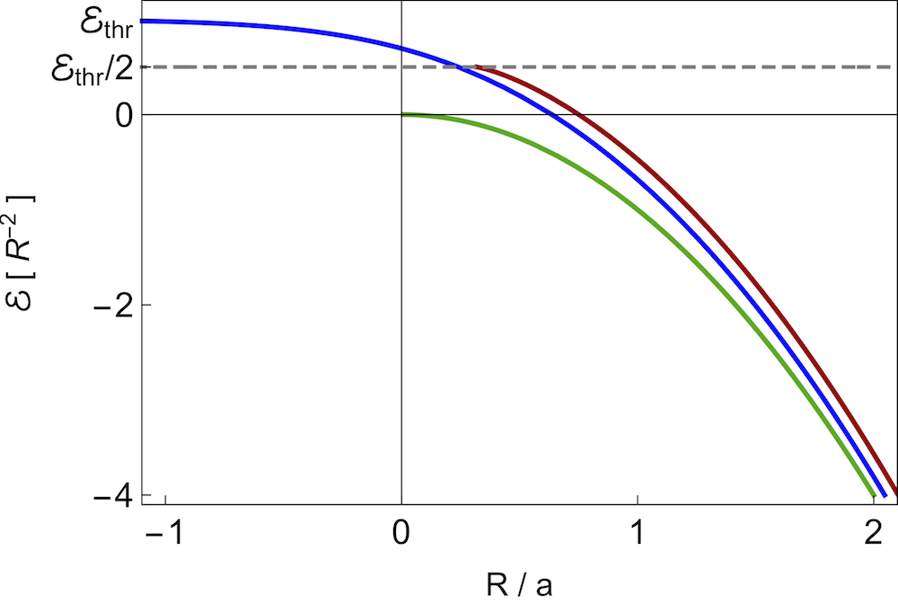
Figure 10: Energy $\mathcal{E}=2\mu E/\hbar^{2}$ in units of $R^{-2}$ vs $R/a$ for two equal-mass atoms with a reduced mass $\mu$ and the s-wave scattering length $a$, where $R$ denotes an arbitrary length scale. The green curve is the result in vacuum, $k_{F}=0$, given by Eq. (A11). The blue curve shows the result of a Cooper pair with vanishing total momentum described by Eq. (15), where both atoms are immersed in an inert Fermi sea with the Fermi momentum $k_{F}R=1$. The red curve is the result for a pair with the total momentum $k_{F}$, where one atom is in vacuum and the other is subject to an inert Fermi sea with the Fermi momentum $k_{F}R=1$; cf. Eqs. (F3) and (F5). The gray dashed lines show $\mathcal{E}_{\mathrm{thr}}$ and $\mathcal{E}_{\mathrm{thr}}/2$, where $\mathcal{E}_{\mathrm{thr}}=2\mu E_{\mathrm{thr}}/\hbar^{2}=k_{F}^{2}$.

To solve Eq. (F1) analytically, we assume s-wave symmetry of the states and consider two cases. For $P_{12}\leqslant(\mu_{12}/m_{1})^{-1}k_{F}$ we have:

$$\frac{4\pi\hbar^{2}}{2\mu_{12}g_{12}}= \frac{-1}{\frac{2\mu_{12}}{m_{1}}\pi P_{12}}\int_{k_{F}-\frac{\mu_{12}}{m_{1}}P_{12}}^{k_{F}+\frac{\mu_{12}}{m_{1}}P_{12}}dp_{12}\,p_{12}$$

$$\times\frac{p_{12}^{2}+(\frac{\mu_{12}}{m_{1}})^{2}P_{12}^{2}-k_{F}^{2}}{p_{12}^{2}+\frac{\mu_{12}}{m_{1}}(1-\frac{\mu_{12}}{m_{1}})P_{12}^{2}-\mathcal{E}_{12}}$$

$$-\frac{1}{\pi}\int_{k_{F}-\frac{\mu_{12}}{m_{1}}P_{12}}^{k_{F}+\frac{\mu_{12}}{m_{1}}P_{12}}dp_{12}\,p_{12}^{2}$$

$$\times\frac{1}{p_{12}^{2}+\frac{\mu_{12}}{m_{1}}(1-\frac{\mu_{12}}{m_{1}})P_{12}^{2}-\mathcal{E}_{12}}$$

$$-\frac{2}{\pi}\int_{k_{F}+\frac{\mu_{12}}{m_{1}}P_{12}}^{\Lambda_{2}}dp_{12}\,p_{12}^{2}$$

$$\times\frac{1}{p_{12}^{2}+\frac{\mu_{12}}{m_{1}}(1-\frac{\mu_{12}}{m_{1}})P_{12}^{2}-\mathcal{E}_{12}}.$$ (F2)

We calculate each integral, take the limit $\Lambda_{2}\rightarrow\infty$, and use Eq. (5). The result is

$$\frac{1}{a_{12}}= \frac{k_{F}}{\pi}-\frac{1}{\pi}\sqrt{\varrho}\left[\arctan\left(\frac{k_{F}-\frac{\mu_{12}}{m_{1}}P_{12}}{\sqrt{\varrho}}\right)\right.$$

$$\left.+\arctan\left(\frac{k_{F}+\frac{\mu_{12}}{m_{1}}P_{12}}{\sqrt{\varrho}}\right)-\pi\right]+\frac{1}{4\pi\frac{\mu_{12}}{m_{1}}P_{12}}$$

$$\times\left(\frac{\mu_{12}}{m_{1}}(\frac{2\mu_{12}}{m_{1}}-1)P_{12}^{2}-k_{F}^{2}+\mathcal{E}_{12}\right)$$

$$\times\ln\left(\frac{\frac{\mu_{12}}{m_{1}}P_{12}^{2}-\frac{2\mu_{12}}{m_{1}}k_{F}P_{12}+k_{F}^{2}-\mathcal{E}_{12}}{\frac{\mu_{12}}{m_{1}}P_{12}^{2}+\frac{2\mu_{12}}{m_{1}}k_{F}P_{12}+k_{F}^{2}-\mathcal{E}_{12}}\right),$$ (F3)

where $\varrho\equiv\frac{\mu_{12}}{m_{1}}(1-\frac{\mu_{12}}{m_{1}})P_{12}^{2}-\mathcal{E}_{12}$ .

For $P_{12}\geqslant(\mu_{12}/m_{1})^{-1}k_{F}$ we have:

$$\frac{4\pi\hbar^{2}}{2\mu_{12}g_{12}}= -\frac{2}{\pi}\int_{0}^{\frac{\mu_{12}}{m_{1}}P_{12}-k_{F}}dp_{12}\,p_{12}^{2}$$

$$\times\frac{1}{p_{12}^{2}+\frac{\mu_{12}}{m_{1}}(1-\frac{\mu_{12}}{m_{1}})P_{12}^{2}-\mathcal{E}_{12}}$$

$$-\frac{1}{\frac{2\mu_{12}}{m_{1}}\pi P_{12}}\int_{\frac{\mu_{12}}{m_{1}}P_{12}-k_{F}}^{\frac{\mu_{12}}{m_{1}}P_{12}+k_{F}}dp_{12}\,p_{12}$$

$$\times\frac{p_{12}^{2}+(\frac{\mu_{12}}{m_{1}})^{2}P_{12}^{2}-k_{F}^{2}}{p_{12}^{2}+\frac{\mu}{m_{1}}(1-\frac{\mu}{m_{1}})P_{12}^{2}-\mathcal{E}_{12}}$$

$$-\frac{1}{\pi}\int_{\frac{\mu_{12}}{m_{1}}P_{12}-k_{F}}^{\frac{\mu_{12}}{m_{1}}P_{12}+k_{F}}dp_{12}\,p_{12}^{2}$$

$$\times\frac{1}{p_{12}^{2}+\frac{\mu_{12}}{m_{1}}(1-\frac{\mu_{12}}{m_{1}})P_{12}^{2}-\mathcal{E}_{12}}$$

$$-\frac{2}{\pi}\int_{\frac{\mu_{12}}{m_{1}}P_{12}+k_{F}}^{\Lambda_{2}}dp_{12}\,p_{12}^{2}$$

$$\times\frac{1}{p_{12}^{2}+\frac{\mu_{12}}{m_{1}}(1-\frac{\mu_{12}}{m_{1}})P_{12}^{2}-\mathcal{E}_{12}}.$$ (F4)

We calculate each integral, take the limit $\Lambda_{2}\rightarrow\infty$, use Eq. (5), and arrive at:

$$\frac{1}{a_{12}}= \frac{k_{F}}{\pi}+\frac{1}{\pi}\sqrt{\varrho}\left[\arctan\left(\frac{\frac{\mu_{12}}{m_{1}}P_{12}-k_{F}}{\sqrt{\varrho}}\right)\right.$$

$$\left.-\arctan\left(\frac{\frac{\mu_{12}}{m_{1}}P_{12}+k_{F}}{\sqrt{\varrho}}\right)+\pi\right]+\frac{1}{4\pi\frac{\mu_{12}}{m_{1}}P_{12}}$$

$$\times\left(\frac{\mu_{12}}{m_{1}}(\frac{2\mu_{12}}{m_{1}}-1)P_{12}^{2}-k_{F}^{2}+\mathcal{E}_{12}\right)$$

$$\times\ln\left(\frac{\frac{\mu_{12}}{m_{1}}P_{12}^{2}-\frac{2\mu_{12}}{m_{1}}k_{F}P_{12}+k_{F}^{2}-\mathcal{E}_{12}}{\frac{\mu_{12}}{m_{1}}P_{12}^{2}+\frac{2\mu_{12}}{m_{1}}k_{F}P_{12}+k_{F}^{2}-\mathcal{E}_{12}}\right);$$ (F5)

see Fig. 10.

As discussed in the text, for $m_{2}/m_{1}\gg 1$ we estimate the onset of a highest-energy excited three-body bound state at zero energy by calculating the onset of the lowest-energy pair-12. To do that, we expand Eq. (F3) or Eq. (F5) for $m_{2}/m_{1}\gg 1$, as $\mathcal{E}_{12}\rightarrow 0$ and $P_{12}\rightarrow(\frac{\mu_{12}}{m_{1}})^{-1}k_{F}$, which results in Eq. (19).

appendix g. calculation of the parameter $s_{0}$

The Efimov scaling factor is $\lambda=\exp(\pi/|s_{0}|)$, where the effect of the mass ratio $m_{2}/m_{1}$ is described by the parameter $s_{0}$. For s-wave symmetry of the states, if we have a system of three species only with two-resonantly interacting pairs, then $s_{0}$ is the purely imaginary root of the transcendental equation

$$\cos\left(\frac{\pi}{2}s_{0}\right)=\frac{2}{\sin 2\vartheta}\frac{\sin(\vartheta s_{0})}{s_{0}},$$ (G1)

where $\vartheta=\arcsin[(m_{2}/m_{1})/(1+m_{2}/m_{1})]$, $\vartheta\in[0,\pi/2]$. If all three species are resonantly interacting, we obtain $s_{0}$ as the purely imaginary root of the equation

$$\left[\cos\left(\frac{\pi}{2}s_{0}\right)-\frac{2}{\sin 2\vartheta}\frac{\sin(\vartheta s_{0})}{s_{0}}\right]\cos\left(\frac{\pi}{2}s_{0}\right)\\ =\frac{8}{\sin^{2}2\gamma}\frac{\sin^{2}(\gamma s_{0})}{s_{0}^{2}},$$ (G2)

where $\gamma=\arcsin\{\sqrt{(m_{1}/m_{2})/[2(1+m_{2}/m_{1})]}\}$, $\gamma\in[0,\pi/4]$. For a proof, see Ref. Pascal_review_paper .