FERMILAB-PUB-20-354-E Published in Phys. Rev. D as DOI: 10.1103/PhysRevD.103.012003

The D0 Collaboration^*^**with visitors from ^aAugustana College, Sioux Falls, SD 57197, USA, ^bThe University of Liverpool, Liverpool L69 3BX, UK, ^cDeutshes Elektronen-Synchrotron (DESY), Notkestrasse 85, Germany, ^dCONACyT, M-03940 Mexico City, Mexico, ^eSLAC, Menlo Park, CA 94025, USA, ^fUniversity College London, London WC1E 6BT, UK, ^gCentro de Investigacion en Computacion - IPN, CP 07738 Mexico City, Mexico, ^hUniversidade Estadual Paulista, São Paulo, SP 01140, Brazil, ⁱKarlsruher Institut für Technologie (KIT) - Steinbuch Centre for Computing (SCC), D-76128 Karlsruhe, Germany, ^jOffice of Science, U.S. Department of Energy, Washington, D.C. 20585, USA, ^kKiev Institute for Nuclear Research (KINR), Kyiv 03680, Ukraine, ^lUniversity of Maryland, College Park, MD 20742, USA, ^mEuropean Orgnaization for Nuclear Research (CERN), CH-1211 Geneva, Switzerland, ⁿPurdue University, West Lafayette, IN 47907, USA, ^oInstitute of Physics, Belgrade, Belgrade, Serbia, and ^pP.N. Lebedev Physical Institute of the Russian Academy of Sciences, 119991, Moscow, Russia. ^‡Deceased.

Study of the normalized transverse momentum distribution of $W$ bosons produced in $p\bar{p}$ collisions at $\sqrt{s}=1.96$ TeV

V.M. Abazov Joint Institute for Nuclear Research, Dubna 141980, Russia B. Abbott University of Oklahoma, Norman, Oklahoma 73019, USA B.S. Acharya Tata Institute of Fundamental Research, Mumbai-400 005, India M. Adams University of Illinois at Chicago, Chicago, Illinois 60607, USA T. Adams Florida State University, Tallahassee, Florida 32306, USA J.P. Agnew The University of Manchester, Manchester M13 9PL, United Kingdom G.D. Alexeev Joint Institute for Nuclear Research, Dubna 141980, Russia G. Alkhazov Petersburg Nuclear Physics Institute, St. Petersburg 188300, Russia A. Alton^a University of Michigan, Ann Arbor, Michigan 48109, USA A. Askew Florida State University, Tallahassee, Florida 32306, USA S. Atkins Louisiana Tech University, Ruston, Louisiana 71272, USA K. Augsten Czech Technical University in Prague, 116 36 Prague 6, Czech Republic V. Aushev Taras Shevchenko National University of Kyiv, Kiev, 01601, Ukraine Y. Aushev Taras Shevchenko National University of Kyiv, Kiev, 01601, Ukraine C. Avila Universidad de los Andes, Bogotá, 111711, Colombia F. Badaud LPC, Université Blaise Pascal, CNRS/IN2P3, Clermont, F-63178 Aubière Cedex, France L. Bagby Fermi National Accelerator Laboratory, Batavia, Illinois 60510, USA B. Baldin Fermi National Accelerator Laboratory, Batavia, Illinois 60510, USA D.V. Bandurin University of Virginia, Charlottesville, Virginia 22904, USA S. Banerjee Tata Institute of Fundamental Research, Mumbai-400 005, India E. Barberis Northeastern University, Boston, Massachusetts 02115, USA P. Baringer University of Kansas, Lawrence, Kansas 66045, USA J.F. Bartlett Fermi National Accelerator Laboratory, Batavia, Illinois 60510, USA U. Bassler IRFU, CEA, Université Paris-Saclay, F-91191 Gif-Sur-Yvette, France V. Bazterra University of Illinois at Chicago, Chicago, Illinois 60607, USA A. Bean University of Kansas, Lawrence, Kansas 66045, USA M. Begalli Universidade do Estado do Rio de Janeiro, Rio de Janeiro, RJ 20550, Brazil L. Bellantoni Fermi National Accelerator Laboratory, Batavia, Illinois 60510, USA S.B. Beri Panjab University, Chandigarh 160014, India G. Bernardi LPNHE, Universités Paris VI and VII, CNRS/IN2P3, F-75005 Paris, France R. Bernhard Physikalisches Institut, Universität Freiburg, 79085 Freiburg, Germany I. Bertram Lancaster University, Lancaster LA1 4YB, United Kingdom M. Besançon IRFU, CEA, Université Paris-Saclay, F-91191 Gif-Sur-Yvette, France R. Beuselinck Imperial College London, London SW7 2AZ, United Kingdom P.C. Bhat Fermi National Accelerator Laboratory, Batavia, Illinois 60510, USA S. Bhatia University of Mississippi, University, Mississippi 38677, USA V. Bhatnagar Panjab University, Chandigarh 160014, India G. Blazey Northern Illinois University, DeKalb, Illinois 60115, USA S. Blessing Florida State University, Tallahassee, Florida 32306, USA K. Bloom University of Nebraska, Lincoln, Nebraska 68588, USA A. Boehnlein Fermi National Accelerator Laboratory, Batavia, Illinois 60510, USA D. Boline State University of New York, Stony Brook, New York 11794, USA E.E. Boos Moscow State University, Moscow 119991, Russia G. Borissov Lancaster University, Lancaster LA1 4YB, United Kingdom M. Borysova^l Taras Shevchenko National University of Kyiv, Kiev, 01601, Ukraine A. Brandt University of Texas, Arlington, Texas 76019, USA O. Brandt II. Physikalisches Institut, Georg-August-Universität Göttingen, 37073 Göttingen, Germany M. Brochmann University of Washington, Seattle, Washington 98195, USA R. Brock Michigan State University, East Lansing, Michigan 48824, USA A. Bross Fermi National Accelerator Laboratory, Batavia, Illinois 60510, USA D. Brown LPNHE, Universités Paris VI and VII, CNRS/IN2P3, F-75005 Paris, France X.B. Bu Fermi National Accelerator Laboratory, Batavia, Illinois 60510, USA M. Buehler Fermi National Accelerator Laboratory, Batavia, Illinois 60510, USA V. Buescher Institut für Physik, Universität Mainz, 55099 Mainz, Germany V. Bunichev Moscow State University, Moscow 119991, Russia S. Burdin^b Lancaster University, Lancaster LA1 4YB, United Kingdom C.P. Buszello Uppsala University, 751 05 Uppsala, Sweden E. Camacho-Pérez CINVESTAV, Mexico City 07360, Mexico B.C.K. Casey Fermi National Accelerator Laboratory, Batavia, Illinois 60510, USA H. Castilla-Valdez CINVESTAV, Mexico City 07360, Mexico S. Caughron Michigan State University, East Lansing, Michigan 48824, USA S. Chakrabarti State University of New York, Stony Brook, New York 11794, USA K.M. Chan University of Notre Dame, Notre Dame, Indiana 46556, USA A. Chandra Rice University, Houston, Texas 77005, USA E. Chapon IRFU, CEA, Université Paris-Saclay, F-91191 Gif-Sur-Yvette, France G. Chen University of Kansas, Lawrence, Kansas 66045, USA S.W. Cho Korea Detector Laboratory, Korea University, Seoul, 02841, Korea S. Choi Korea Detector Laboratory, Korea University, Seoul, 02841, Korea B. Choudhary Delhi University, Delhi-110 007, India S. Cihangir^‡ Fermi National Accelerator Laboratory, Batavia, Illinois 60510, USA D. Claes University of Nebraska, Lincoln, Nebraska 68588, USA J. Clutter University of Kansas, Lawrence, Kansas 66045, USA M. Cooke^j Fermi National Accelerator Laboratory, Batavia, Illinois 60510, USA W.E. Cooper Fermi National Accelerator Laboratory, Batavia, Illinois 60510, USA M. Corcoran^‡ Rice University, Houston, Texas 77005, USA F. Couderc IRFU, CEA, Université Paris-Saclay, F-91191 Gif-Sur-Yvette, France M.-C. Cousinou CPPM, Aix-Marseille Université, CNRS/IN2P3, F-13288 Marseille Cedex 09, France J. Cuth Institut für Physik, Universität Mainz, 55099 Mainz, Germany D. Cutts Brown University, Providence, Rhode Island 02912, USA A. Das Southern Methodist University, Dallas, Texas 75275, USA G. Davies Imperial College London, London SW7 2AZ, United Kingdom S.J. de Jong Nikhef, Science Park, 1098 XG Amsterdam, the Netherlands Radboud University Nijmegen, 6525 AJ Nijmegen, the Netherlands E. De La Cruz-Burelo CINVESTAV, Mexico City 07360, Mexico F. Déliot IRFU, CEA, Université Paris-Saclay, F-91191 Gif-Sur-Yvette, France R. Demina University of Rochester, Rochester, New York 14627, USA D. Denisov Brookhaven National Laboratory, Upton, New York 11973, USA S.P. Denisov Institute for High Energy Physics, Protvino, Moscow region 142281, Russia S. Desai Fermi National Accelerator Laboratory, Batavia, Illinois 60510, USA C. Deterre^c The University of Manchester, Manchester M13 9PL, United Kingdom K. DeVaughan University of Nebraska, Lincoln, Nebraska 68588, USA H.T. Diehl Fermi National Accelerator Laboratory, Batavia, Illinois 60510, USA M. Diesburg Fermi National Accelerator Laboratory, Batavia, Illinois 60510, USA P.F. Ding The University of Manchester, Manchester M13 9PL, United Kingdom A. Dominguez University of Nebraska, Lincoln, Nebraska 68588, USA A. Drutskoy^q Institute for Theoretical and Experimental Physics, Moscow 117259, Russia A. Dubey Delhi University, Delhi-110 007, India L.V. Dudko Moscow State University, Moscow 119991, Russia A. Duperrin CPPM, Aix-Marseille Université, CNRS/IN2P3, F-13288 Marseille Cedex 09, France S. Dutt Panjab University, Chandigarh 160014, India M. Eads Northern Illinois University, DeKalb, Illinois 60115, USA D. Edmunds Michigan State University, East Lansing, Michigan 48824, USA J. Ellison University of California Riverside, Riverside, California 92521, USA V.D. Elvira Fermi National Accelerator Laboratory, Batavia, Illinois 60510, USA Y. Enari LPNHE, Universités Paris VI and VII, CNRS/IN2P3, F-75005 Paris, France H. Evans Indiana University, Bloomington, Indiana 47405, USA A. Evdokimov University of Illinois at Chicago, Chicago, Illinois 60607, USA V.N. Evdokimov Institute for High Energy Physics, Protvino, Moscow region 142281, Russia A. Fauré IRFU, CEA, Université Paris-Saclay, F-91191 Gif-Sur-Yvette, France L. Feng Northern Illinois University, DeKalb, Illinois 60115, USA T. Ferbel University of Rochester, Rochester, New York 14627, USA F. Fiedler Institut für Physik, Universität Mainz, 55099 Mainz, Germany F. Filthaut Nikhef, Science Park, 1098 XG Amsterdam, the Netherlands Radboud University Nijmegen, 6525 AJ Nijmegen, the Netherlands W. Fisher Michigan State University, East Lansing, Michigan 48824, USA H.E. Fisk Fermi National Accelerator Laboratory, Batavia, Illinois 60510, USA M. Fortner Northern Illinois University, DeKalb, Illinois 60115, USA H. Fox Lancaster University, Lancaster LA1 4YB, United Kingdom J. Franc Czech Technical University in Prague, 116 36 Prague 6, Czech Republic S. Fuess Fermi National Accelerator Laboratory, Batavia, Illinois 60510, USA Y. Fu University of Science and Technology of China, Hefei 230026, People’s Republic of China P.H. Garbincius Fermi National Accelerator Laboratory, Batavia, Illinois 60510, USA A. Garcia-Bellido University of Rochester, Rochester, New York 14627, USA J.A. García-González CINVESTAV, Mexico City 07360, Mexico V. Gavrilov Institute for Theoretical and Experimental Physics, Moscow 117259, Russia W. Geng CPPM, Aix-Marseille Université, CNRS/IN2P3, F-13288 Marseille Cedex 09, France Michigan State University, East Lansing, Michigan 48824, USA C.E. Gerber University of Illinois at Chicago, Chicago, Illinois 60607, USA Y. Gershtein Rutgers University, Piscataway, New Jersey 08855, USA G. Ginther Fermi National Accelerator Laboratory, Batavia, Illinois 60510, USA O. Gogota Taras Shevchenko National University of Kyiv, Kiev, 01601, Ukraine G. Golovanov Joint Institute for Nuclear Research, Dubna 141980, Russia P.D. Grannis State University of New York, Stony Brook, New York 11794, USA S. Greder IPHC, Université de Strasbourg, CNRS/IN2P3, F-67037 Strasbourg, France H. Greenlee Fermi National Accelerator Laboratory, Batavia, Illinois 60510, USA G. Grenier IPNL, Université Lyon 1, CNRS/IN2P3, F-69622 Villeurbanne Cedex, France and Université de Lyon, F-69361 Lyon CEDEX 07, France Ph. Gris LPC, Université Blaise Pascal, CNRS/IN2P3, Clermont, F-63178 Aubière Cedex, France J.-F. Grivaz LAL, Univ. Paris-Sud, CNRS/IN2P3, Université Paris-Saclay, F-91898 Orsay Cedex, France A. Grohsjean^c IRFU, CEA, Université Paris-Saclay, F-91191 Gif-Sur-Yvette, France S. Grünendahl Fermi National Accelerator Laboratory, Batavia, Illinois 60510, USA M.W. Grünewald University College Dublin, Dublin 4, Ireland T. Guillemin LAL, Univ. Paris-Sud, CNRS/IN2P3, Université Paris-Saclay, F-91898 Orsay Cedex, France G. Gutierrez Fermi National Accelerator Laboratory, Batavia, Illinois 60510, USA P. Gutierrez University of Oklahoma, Norman, Oklahoma 73019, USA J. Haley Oklahoma State University, Stillwater, Oklahoma 74078, USA L. Han University of Science and Technology of China, Hefei 230026, People’s Republic of China K. Harder The University of Manchester, Manchester M13 9PL, United Kingdom A. Harel University of Rochester, Rochester, New York 14627, USA J.M. Hauptman Iowa State University, Ames, Iowa 50011, USA J. Hays Imperial College London, London SW7 2AZ, United Kingdom T. Head The University of Manchester, Manchester M13 9PL, United Kingdom T. Hebbeker III. Physikalisches Institut A, RWTH Aachen University, 52056 Aachen, Germany D. Hedin Northern Illinois University, DeKalb, Illinois 60115, USA H. Hegab Oklahoma State University, Stillwater, Oklahoma 74078, USA A.P. Heinson University of California Riverside, Riverside, California 92521, USA U. Heintz Brown University, Providence, Rhode Island 02912, USA C. Hensel LAFEX, Centro Brasileiro de Pesquisas Físicas, Rio de Janeiro, RJ 22290, Brazil I. Heredia-De La Cruz^d CINVESTAV, Mexico City 07360, Mexico K. Herner Fermi National Accelerator Laboratory, Batavia, Illinois 60510, USA G. Hesketh^f The University of Manchester, Manchester M13 9PL, United Kingdom M.D. Hildreth University of Notre Dame, Notre Dame, Indiana 46556, USA R. Hirosky University of Virginia, Charlottesville, Virginia 22904, USA T. Hoang Florida State University, Tallahassee, Florida 32306, USA J.D. Hobbs State University of New York, Stony Brook, New York 11794, USA B. Hoeneisen Universidad San Francisco de Quito, Quito 170157, Ecuador J. Hogan Rice University, Houston, Texas 77005, USA M. Hohlfeld Institut für Physik, Universität Mainz, 55099 Mainz, Germany J.L. Holzbauer University of Mississippi, University, Mississippi 38677, USA I. Howley University of Texas, Arlington, Texas 76019, USA Z. Hubacek Czech Technical University in Prague, 116 36 Prague 6, Czech Republic IRFU, CEA, Université Paris-Saclay, F-91191 Gif-Sur-Yvette, France V. Hynek Czech Technical University in Prague, 116 36 Prague 6, Czech Republic I. Iashvili State University of New York, Buffalo, New York 14260, USA Y. Ilchenko Southern Methodist University, Dallas, Texas 75275, USA R. Illingworth Fermi National Accelerator Laboratory, Batavia, Illinois 60510, USA A.S. Ito Fermi National Accelerator Laboratory, Batavia, Illinois 60510, USA S. Jabeen^m Fermi National Accelerator Laboratory, Batavia, Illinois 60510, USA M. Jaffré LAL, Univ. Paris-Sud, CNRS/IN2P3, Université Paris-Saclay, F-91898 Orsay Cedex, France A. Jayasinghe University of Oklahoma, Norman, Oklahoma 73019, USA M.S. Jeong Korea Detector Laboratory, Korea University, Seoul, 02841, Korea R. Jesik Imperial College London, London SW7 2AZ, United Kingdom P. Jiang^‡ University of Science and Technology of China, Hefei 230026, People’s Republic of China K. Johns University of Arizona, Tucson, Arizona 85721, USA E. Johnson Michigan State University, East Lansing, Michigan 48824, USA M. Johnson Fermi National Accelerator Laboratory, Batavia, Illinois 60510, USA A. Jonckheere Fermi National Accelerator Laboratory, Batavia, Illinois 60510, USA P. Jonsson Imperial College London, London SW7 2AZ, United Kingdom J. Joshi University of California Riverside, Riverside, California 92521, USA A.W. Jung^o Fermi National Accelerator Laboratory, Batavia, Illinois 60510, USA A. Juste Institució Catalana de Recerca i Estudis Avançats (ICREA) and Institut de Física d’Altes Energies (IFAE), 08193 Bellaterra (Barcelona), Spain E. Kajfasz CPPM, Aix-Marseille Université, CNRS/IN2P3, F-13288 Marseille Cedex 09, France D. Karmanov Moscow State University, Moscow 119991, Russia I. Katsanos University of Nebraska, Lincoln, Nebraska 68588, USA M. Kaur Panjab University, Chandigarh 160014, India R. Kehoe Southern Methodist University, Dallas, Texas 75275, USA S. Kermiche CPPM, Aix-Marseille Université, CNRS/IN2P3, F-13288 Marseille Cedex 09, France N. Khalatyan Fermi National Accelerator Laboratory, Batavia, Illinois 60510, USA A. Khanov Oklahoma State University, Stillwater, Oklahoma 74078, USA A. Kharchilava State University of New York, Buffalo, New York 14260, USA Y.N. Kharzheev Joint Institute for Nuclear Research, Dubna 141980, Russia I. Kiselevich Institute for Theoretical and Experimental Physics, Moscow 117259, Russia J.M. Kohli Panjab University, Chandigarh 160014, India A.V. Kozelov Institute for High Energy Physics, Protvino, Moscow region 142281, Russia J. Kraus University of Mississippi, University, Mississippi 38677, USA A. Kumar State University of New York, Buffalo, New York 14260, USA A. Kupco Institute of Physics, Academy of Sciences of the Czech Republic, 182 21 Prague, Czech Republic T. Kurča IPNL, Université Lyon 1, CNRS/IN2P3, F-69622 Villeurbanne Cedex, France and Université de Lyon, F-69361 Lyon CEDEX 07, France V.A. Kuzmin Moscow State University, Moscow 119991, Russia S. Lammers Indiana University, Bloomington, Indiana 47405, USA P. Lebrun IPNL, Université Lyon 1, CNRS/IN2P3, F-69622 Villeurbanne Cedex, France and Université de Lyon, F-69361 Lyon CEDEX 07, France H.S. Lee Korea Detector Laboratory, Korea University, Seoul, 02841, Korea S.W. Lee Iowa State University, Ames, Iowa 50011, USA W.M. Lee^‡ Fermi National Accelerator Laboratory, Batavia, Illinois 60510, USA X. Lei University of Arizona, Tucson, Arizona 85721, USA J. Lellouch LPNHE, Universités Paris VI and VII, CNRS/IN2P3, F-75005 Paris, France D. Li LPNHE, Universités Paris VI and VII, CNRS/IN2P3, F-75005 Paris, France H. Li University of Virginia, Charlottesville, Virginia 22904, USA L. Li University of California Riverside, Riverside, California 92521, USA Q.Z. Li Fermi National Accelerator Laboratory, Batavia, Illinois 60510, USA J.K. Lim Korea Detector Laboratory, Korea University, Seoul, 02841, Korea D. Lincoln Fermi National Accelerator Laboratory, Batavia, Illinois 60510, USA J. Linnemann Michigan State University, East Lansing, Michigan 48824, USA V.V. Lipaev^‡ Institute for High Energy Physics, Protvino, Moscow region 142281, Russia R. Lipton Fermi National Accelerator Laboratory, Batavia, Illinois 60510, USA H. Liu Southern Methodist University, Dallas, Texas 75275, USA Y. Liu University of Science and Technology of China, Hefei 230026, People’s Republic of China A. Lobodenko Petersburg Nuclear Physics Institute, St. Petersburg 188300, Russia M. Lokajicek Institute of Physics, Academy of Sciences of the Czech Republic, 182 21 Prague, Czech Republic R. Lopes de Sa Fermi National Accelerator Laboratory, Batavia, Illinois 60510, USA R. Luna-Garcia^g CINVESTAV, Mexico City 07360, Mexico A.L. Lyon Fermi National Accelerator Laboratory, Batavia, Illinois 60510, USA A.K.A. Maciel LAFEX, Centro Brasileiro de Pesquisas Físicas, Rio de Janeiro, RJ 22290, Brazil R. Madar Physikalisches Institut, Universität Freiburg, 79085 Freiburg, Germany R. Magaña-Villalba CINVESTAV, Mexico City 07360, Mexico S. Malik University of Nebraska, Lincoln, Nebraska 68588, USA V.L. Malyshev Joint Institute for Nuclear Research, Dubna 141980, Russia J. Mansour II. Physikalisches Institut, Georg-August-Universität Göttingen, 37073 Göttingen, Germany J. Martínez-Ortega CINVESTAV, Mexico City 07360, Mexico R. McCarthy State University of New York, Stony Brook, New York 11794, USA C.L. McGivern The University of Manchester, Manchester M13 9PL, United Kingdom M.M. Meijer Nikhef, Science Park, 1098 XG Amsterdam, the Netherlands Radboud University Nijmegen, 6525 AJ Nijmegen, the Netherlands A. Melnitchouk Fermi National Accelerator Laboratory, Batavia, Illinois 60510, USA D. Menezes Northern Illinois University, DeKalb, Illinois 60115, USA P.G. Mercadante Universidade Federal do ABC, Santo André, SP 09210, Brazil M. Merkin Moscow State University, Moscow 119991, Russia A. Meyer III. Physikalisches Institut A, RWTH Aachen University, 52056 Aachen, Germany J. Meyerⁱ II. Physikalisches Institut, Georg-August-Universität Göttingen, 37073 Göttingen, Germany F. Miconi IPHC, Université de Strasbourg, CNRS/IN2P3, F-67037 Strasbourg, France N.K. Mondal Tata Institute of Fundamental Research, Mumbai-400 005, India M. Mulhearn University of Virginia, Charlottesville, Virginia 22904, USA E. Nagy CPPM, Aix-Marseille Université, CNRS/IN2P3, F-13288 Marseille Cedex 09, France M. Narain Brown University, Providence, Rhode Island 02912, USA R. Nayyar University of Arizona, Tucson, Arizona 85721, USA H.A. Neal^‡ University of Michigan, Ann Arbor, Michigan 48109, USA J.P. Negret Universidad de los Andes, Bogotá, 111711, Colombia P. Neustroev Petersburg Nuclear Physics Institute, St. Petersburg 188300, Russia H.T. Nguyen University of Virginia, Charlottesville, Virginia 22904, USA T. Nunnemann Ludwig-Maximilians-Universität München, 80539 München, Germany J. Orduna Brown University, Providence, Rhode Island 02912, USA N. Osman CPPM, Aix-Marseille Université, CNRS/IN2P3, F-13288 Marseille Cedex 09, France A. Pal University of Texas, Arlington, Texas 76019, USA N. Parashar Purdue University Calumet, Hammond, Indiana 46323, USA V. Parihar Brown University, Providence, Rhode Island 02912, USA S.K. Park Korea Detector Laboratory, Korea University, Seoul, 02841, Korea R. Partridge^e Brown University, Providence, Rhode Island 02912, USA N. Parua Indiana University, Bloomington, Indiana 47405, USA A. Patwa^j Brookhaven National Laboratory, Upton, New York 11973, USA B. Penning Imperial College London, London SW7 2AZ, United Kingdom M. Perfilov Moscow State University, Moscow 119991, Russia Y. Peters The University of Manchester, Manchester M13 9PL, United Kingdom K. Petridis The University of Manchester, Manchester M13 9PL, United Kingdom G. Petrillo University of Rochester, Rochester, New York 14627, USA P. Pétroff LAL, Univ. Paris-Sud, CNRS/IN2P3, Université Paris-Saclay, F-91898 Orsay Cedex, France M.-A. Pleier Brookhaven National Laboratory, Upton, New York 11973, USA V.M. Podstavkov Fermi National Accelerator Laboratory, Batavia, Illinois 60510, USA A.V. Popov Institute for High Energy Physics, Protvino, Moscow region 142281, Russia M. Prewitt Rice University, Houston, Texas 77005, USA D. Price The University of Manchester, Manchester M13 9PL, United Kingdom N. Prokopenko Institute for High Energy Physics, Protvino, Moscow region 142281, Russia J. Qian University of Michigan, Ann Arbor, Michigan 48109, USA A. Quadt II. Physikalisches Institut, Georg-August-Universität Göttingen, 37073 Göttingen, Germany B. Quinn University of Mississippi, University, Mississippi 38677, USA P.N. Ratoff Lancaster University, Lancaster LA1 4YB, United Kingdom I. Razumov Institute for High Energy Physics, Protvino, Moscow region 142281, Russia I. Ripp-Baudot IPHC, Université de Strasbourg, CNRS/IN2P3, F-67037 Strasbourg, France F. Rizatdinova Oklahoma State University, Stillwater, Oklahoma 74078, USA M. Rominsky Fermi National Accelerator Laboratory, Batavia, Illinois 60510, USA A. Ross Lancaster University, Lancaster LA1 4YB, United Kingdom C. Royon Institute of Physics, Academy of Sciences of the Czech Republic, 182 21 Prague, Czech Republic P. Rubinov Fermi National Accelerator Laboratory, Batavia, Illinois 60510, USA R. Ruchti University of Notre Dame, Notre Dame, Indiana 46556, USA G. Sajot LPSC, Université Joseph Fourier Grenoble 1, CNRS/IN2P3, Institut National Polytechnique de Grenoble, F-38026 Grenoble Cedex, France A. Sánchez-Hernández CINVESTAV, Mexico City 07360, Mexico M.P. Sanders Ludwig-Maximilians-Universität München, 80539 München, Germany A.S. Santos^h LAFEX, Centro Brasileiro de Pesquisas Físicas, Rio de Janeiro, RJ 22290, Brazil G. Savage Fermi National Accelerator Laboratory, Batavia, Illinois 60510, USA M. Savitskyi Taras Shevchenko National University of Kyiv, Kiev, 01601, Ukraine L. Sawyer Louisiana Tech University, Ruston, Louisiana 71272, USA T. Scanlon Imperial College London, London SW7 2AZ, United Kingdom R.D. Schamberger State University of New York, Stony Brook, New York 11794, USA Y. Scheglov^‡ Petersburg Nuclear Physics Institute, St. Petersburg 188300, Russia H. Schellman Oregon State University, Corvallis, Oregon 97331, USA Northwestern University, Evanston, Illinois 60208, USA M. Schott Institut für Physik, Universität Mainz, 55099 Mainz, Germany C. Schwanenberger^c The University of Manchester, Manchester M13 9PL, United Kingdom R. Schwienhorst Michigan State University, East Lansing, Michigan 48824, USA J. Sekaric University of Kansas, Lawrence, Kansas 66045, USA H. Severini University of Oklahoma, Norman, Oklahoma 73019, USA E. Shabalina II. Physikalisches Institut, Georg-August-Universität Göttingen, 37073 Göttingen, Germany V. Shary IRFU, CEA, Université Paris-Saclay, F-91191 Gif-Sur-Yvette, France S. Shaw The University of Manchester, Manchester M13 9PL, United Kingdom A.A. Shchukin Institute for High Energy Physics, Protvino, Moscow region 142281, Russia O. Shkola Taras Shevchenko National University of Kyiv, Kiev, 01601, Ukraine V. Simak^‡ Czech Technical University in Prague, 116 36 Prague 6, Czech Republic P. Skubic University of Oklahoma, Norman, Oklahoma 73019, USA P. Slattery University of Rochester, Rochester, New York 14627, USA G.R. Snow^‡ University of Nebraska, Lincoln, Nebraska 68588, USA J. Snow Langston University, Langston, Oklahoma 73050, USA S. Snyder Brookhaven National Laboratory, Upton, New York 11973, USA S. Söldner-Rembold The University of Manchester, Manchester M13 9PL, United Kingdom L. Sonnenschein III. Physikalisches Institut A, RWTH Aachen University, 52056 Aachen, Germany K. Soustruznik Charles University, Faculty of Mathematics and Physics, Center for Particle Physics, 116 36 Prague 1, Czech Republic J. Stark LPSC, Université Joseph Fourier Grenoble 1, CNRS/IN2P3, Institut National Polytechnique de Grenoble, F-38026 Grenoble Cedex, France N. Stefaniuk Taras Shevchenko National University of Kyiv, Kiev, 01601, Ukraine D.A. Stoyanova Institute for High Energy Physics, Protvino, Moscow region 142281, Russia M. Strauss University of Oklahoma, Norman, Oklahoma 73019, USA L. Suter The University of Manchester, Manchester M13 9PL, United Kingdom P. Svoisky University of Virginia, Charlottesville, Virginia 22904, USA M. Titov IRFU, CEA, Université Paris-Saclay, F-91191 Gif-Sur-Yvette, France V.V. Tokmenin Joint Institute for Nuclear Research, Dubna 141980, Russia Y.-T. Tsai University of Rochester, Rochester, New York 14627, USA D. Tsybychev State University of New York, Stony Brook, New York 11794, USA B. Tuchming IRFU, CEA, Université Paris-Saclay, F-91191 Gif-Sur-Yvette, France C. Tully Princeton University, Princeton, New Jersey 08544, USA L. Uvarov Petersburg Nuclear Physics Institute, St. Petersburg 188300, Russia S. Uvarov Petersburg Nuclear Physics Institute, St. Petersburg 188300, Russia S. Uzunyan Northern Illinois University, DeKalb, Illinois 60115, USA R. Van Kooten Indiana University, Bloomington, Indiana 47405, USA W.M. van Leeuwen Nikhef, Science Park, 1098 XG Amsterdam, the Netherlands N. Varelas University of Illinois at Chicago, Chicago, Illinois 60607, USA E.W. Varnes University of Arizona, Tucson, Arizona 85721, USA I.A. Vasilyev Institute for High Energy Physics, Protvino, Moscow region 142281, Russia A.Y. Verkheev Joint Institute for Nuclear Research, Dubna 141980, Russia L.S. Vertogradov Joint Institute for Nuclear Research, Dubna 141980, Russia M. Verzocchi Fermi National Accelerator Laboratory, Batavia, Illinois 60510, USA M. Vesterinen The University of Manchester, Manchester M13 9PL, United Kingdom D. Vilanova IRFU, CEA, Université Paris-Saclay, F-91191 Gif-Sur-Yvette, France P. Vokac Czech Technical University in Prague, 116 36 Prague 6, Czech Republic H.D. Wahl Florida State University, Tallahassee, Florida 32306, USA C. Wang University of Science and Technology of China, Hefei 230026, People’s Republic of China M.H.L.S. Wang Fermi National Accelerator Laboratory, Batavia, Illinois 60510, USA J. Warchol^‡ University of Notre Dame, Notre Dame, Indiana 46556, USA G. Watts University of Washington, Seattle, Washington 98195, USA M. Wayne University of Notre Dame, Notre Dame, Indiana 46556, USA J. Weichert Institut für Physik, Universität Mainz, 55099 Mainz, Germany L. Welty-Rieger Northwestern University, Evanston, Illinois 60208, USA M.R.J. Williamsⁿ Indiana University, Bloomington, Indiana 47405, USA G.W. Wilson University of Kansas, Lawrence, Kansas 66045, USA M. Wobisch Louisiana Tech University, Ruston, Louisiana 71272, USA D.R. Wood Northeastern University, Boston, Massachusetts 02115, USA T.R. Wyatt The University of Manchester, Manchester M13 9PL, United Kingdom Y. Xie Fermi National Accelerator Laboratory, Batavia, Illinois 60510, USA R. Yamada Fermi National Accelerator Laboratory, Batavia, Illinois 60510, USA S. Yang University of Science and Technology of China, Hefei 230026, People’s Republic of China T. Yasuda Fermi National Accelerator Laboratory, Batavia, Illinois 60510, USA Y.A. Yatsunenko Joint Institute for Nuclear Research, Dubna 141980, Russia W. Ye State University of New York, Stony Brook, New York 11794, USA Z. Ye Fermi National Accelerator Laboratory, Batavia, Illinois 60510, USA H. Yin Fermi National Accelerator Laboratory, Batavia, Illinois 60510, USA K. Yip Brookhaven National Laboratory, Upton, New York 11973, USA S.W. Youn Fermi National Accelerator Laboratory, Batavia, Illinois 60510, USA J.M. Yu University of Michigan, Ann Arbor, Michigan 48109, USA J. Zennamo State University of New York, Buffalo, New York 14260, USA T.G. Zhao The University of Manchester, Manchester M13 9PL, United Kingdom B. Zhou University of Michigan, Ann Arbor, Michigan 48109, USA J. Zhu University of Michigan, Ann Arbor, Michigan 48109, USA M. Zielinski University of Rochester, Rochester, New York 14627, USA D. Zieminska Indiana University, Bloomington, Indiana 47405, USA L. Zivkovic^p LPNHE, Universités Paris VI and VII, CNRS/IN2P3, F-75005 Paris, France

Abstract

We present a study of the normalized transverse momentum distribution of $W$ bosons produced in $p\bar{p}$ collisions, using data corresponding to an integrated luminosity of 4.35 fb^-1 collected with the D0 detector at the Fermilab Tevatron collider at $\sqrt{s}=1.96$ TeV. The measurement focuses on the transverse momentum region below 15 GeV, which is of special interest for electroweak precision measurements; it relies on the same detector calibration methods which were used for the precision measurement of the $W$ boson mass. The measured distribution is compared to different QCD predictions and a procedure is given to allow the comparison of any further theoretical models to the D0 data.

pacs:

14.70.Fm, 13.85.Qk, 12.38.Qk

I. INTRODUCTION

The production of $V=(W/Z)$ bosons in hadron collisions is described by perturbative quantum chromodynamics (QCD). At leading order, QCD predicts no transverse momentum of the $W$ or $Z$ boson ( $p_{T}^{V}$ ) with respect to the beam direction ATLASReview . However, this changes when including higher order corrections, so that significant $p_{T}^{V}$ can arise from the emission of partons in the initial state as well as from the intrinsic transverse momentum of the initial-state partons in the proton. The $p_{T}^{V}$ spectrum at low transverse momentum can be described using soft-gluon resummation Collins:1984kg ; Balazs:1997xd ; Becher:2010tm ; Catani:2015vma ; Ebert:2016gcn ; Bizon:2017rah , parton shower approaches Bellm:2015jjp ; Sjostrand:2014zea ; Bothmann:2019yzt , and non-perturbative calculations NPQCD ; NPFunc to account for the intrinsic transverse momentum of partons. In the non-perturbative approach NPQCD ; NPFunc , a function is introduced as a form factor in order to make the QCD calculation convergent when $p_{T}^{V}\rightarrow 0^{+}$ . The values of the parameters in the non-perturbative function can only be extracted from the measurement of the $p_{T}^{V}$ distribution. Knowledge of the $p_{T}^{V}$ spectrum is not only important for testing perturbative QCD predictions and constraining models of non-perturbative approaches, but also for the measurement of electroweak parameters such as the $W$ boson mass. In the latter case, it is especially important to model the $p_{T}^{W}$ spectrum correctly in the low $p_{T}$ region.

The transverse momentum spectrum of the $Z$ boson has been measured to high precision at various energies, both at the Tevatron DZeroZPt1 ; DZeroZPt2 ; DZeroZPt3 ; CDFZPt and the LHC ATLASZPt1 ; ATLASZPt2 ; ATLASZPt3 ; CMSZPt1 ; CMSZPt2 ; CMSPt . This precision is enabled by the fact that leptonically-decaying $Z$ bosons can be easily reconstructed from the two charged leptons in the final state. The situation is different for the $W$ boson as the neutrino escapes detection and hadronic decays have large backgrounds. The $p_{T}^{W}$ must therefore be estimated from the reconstructed hadronic recoil of the event. The hadronic recoil is only an approximation of $p_{T}(W)$ as it is significantly affected by the number of simultaneous hadron collisions in the recorded event and by the non-linear energy response of the detector for low energy hadrons.

The $p_{T}^{W}$ distribution was previously measured at the Tevatron at $\sqrt{s}=1.8$ TeV DZeroWPt1 ; DZeroWPt2 , and at the LHC at $\sqrt{s}=7$ and $8$ TeV ATLASWPt ; CMSPt . This study is the first $p_{T}^{W}$ analysis at $\sqrt{s}=1.96$ TeV. In this paper, we analyze data corresponding to an integrated luminosity of 4.35 fb^-1 collected by the D0 detector at the Fermilab Tevatron collider. These data were also used for the $W$ boson mass measurement in Ref. WMass . This study concentrates on the low $p_{T}^{W}$ region and resolves the peak near $p_{T}^{W}=4$ GeV, unlike the LHC measurements of Refs. ATLASWPt ; CMSPt where the sizes of the first bin are 8 GeV and 7.5 GeV, respectively. In addition, we study the transverse momentum of $W$ bosons in the case where the production is dominated by valence quarks, unlike the situation at the LHC which involves sea quarks. Typical Bjorken $x$ -values for $W$ boson production at the Tevatron (LHC) are 0.05 (0.015) ATLASReview .

This paper is structured as follows: after a short description of the D0 detector, the event selection, the calibration procedure, and the basic comparison plots between data and simulation are presented. This is followed by a description of the analysis procedure. After a discussion of the systematic uncertainties, the final results are presented and compared with several models of $W$ boson production and parton distribution functions. Finally, a fast folding procedure is introduced in the appendix, which can be used to compare our result to other theoretical predictions while properly accounting for the detector response.

II. THE D0 DETECTOR

The D0 detector d0-detector comprises a central tracking system, a calorimeter, and a muon system. The analysis uses a cylindrical coordinate system with the $z$ axis along the beam axis in the proton direction. Angles $\theta$ and $\phi$ are the polar and azimuthal angles, respectively. Pseudorapidity is defined as $\eta=-\ln[\tan(\theta/2)]$ where $\theta$ is measured with respect to the interaction vertex. We define $\eta_{\text{det}}$ as the pseudorapidity measured with respect to the center of the detector. The central tracking system consists of a silicon microstrip tracker (SMT) and a scintillating fiber tracker, both located within a 1.9 T superconducting solenoid magnet and optimized for tracking and vertexing for $|\eta_{\text{det}}|<2.5$ . Outside the solenoid, liquid argon and uranium calorimeters provide energy measurement, with a central calorimeter (CC) that covers $|\eta_{\text{det}}|\leq 1.05$ , and two end calorimeters (EC) that extend coverage to $|\eta_{\text{det}}|<4.2$ . The muon system located outside the calorimeter consists of drift tubes and scintillators before and after 1.8 T iron toroid magnets and provides coverage for $|\eta_{\text{det}}|<2.0$ . Muons are identified and their momenta are measured using information from both the tracking system and the muon system. The solenoid and toroid polarities are reversed every two weeks on average during the periods of data-taking.

III. EVENT SAMPLES AND EVENT SELECTION

The present analysis builds on the techniques developed in Refs. WMass and D0NewW for the measurement of the $W$ boson mass. Events are selected using a trigger requiring at least one electromagnetic (EM) cluster found in the CC, with the transverse energy threshold varying from 25 to 27 GeV depending on run conditions. The offline selection of candidate $W$ boson events is the same as used in Ref. WMass . We require candidate electrons to be matched in $(\eta,\phi)$ space to a track including at least one SMT hit. The electron three-momentum vector magnitude is defined by the cluster energy, and the direction is defined by the track.

We require the presence of an electron with $p_{T}^{e}>25$ GeV and $|\eta^{e}|<1.05$ that passes shower shape and isolation requirements. Here $p_{T}^{e}$ is the magnitude of the transverse momentum of the electron, $\vec{p}_{T}^{~{}e}$ , and $\eta^{e}$ is the pseudorapidity of the electron. The event must satisfy $~{}{/\kern-6.99997ptE}_{T}>25$ GeV, $u_{T}<15$ GeV, and $50<m_{T}<200$ GeV. Here, the hadronic recoil $\vec{u}_{T}$ is the vector sum of the transverse component of the energies measured in calorimeter cells excluding those associated with the reconstructed electron, and $u_{T}$ is its magnitude. The relation $~{}\vec{/\kern-6.99997ptE}_{T}=-(\vec{p}_{T}^{~{}e}+\vec{u}_{T})$ defines the missing transverse energy approximating the transverse momentum of the neutrino, and $m_{T}$ is the transverse mass defined as $m_{T}=\sqrt{2p_{T}^{e}{/\kern-6.99997ptE}_{T}(1-\cos\Delta\phi)}$ , where $\Delta\phi$ is the azimuthal opening angle between $\vec{p}_{T}^{~{}e}$ and $\vec{/\kern-6.99997ptE}_{T}$ . This selection yields 1 677 394 candidate $W\to e\nu$ events.

The $Z\to ee$ events were used extensively to calibrate the detector response D0NewW ; WMass , and they are also used in this study. These events are required to have two EM clusters satisfying the $W$ candidate cluster requirements above, except that one of the two clusters may be reconstructed within an EC $(1.5<|\eta|<2.5)$ . The associated tracks must be of opposite curvature. The $Z$ boson events must also have $u_{T}<15$ GeV and $70\leq m_{ee}\leq 110$ GeV, where $m_{ee}$ is the invariant mass of the electron-positron pair.

The resbos Balazs:1997xd event generator, combined with photos photos , is used as a baseline simulation for the kinematics of $W$ and $Z$ boson production and decay. resbos is a next-to-leading order event generator including next-to-next-to-leading logarithm resummation of soft gluons Collins:1984kg , and photos generates up to two final state radiated photons. At low transverse momentum ( $p_{T}^{V}<10$ GeV), multiple soft gluon emissions dominate the cross section and a soft-gluon resummation formalism is used to make QCD predictions. This technique was first developed by Collins, Soper, and Sterman (CSS) Collins:1984kg and is currently implemented using a parametric function introduced by Brock, Landry, Nadolsky and Yuan (BLNY) g2 based on three non-perturbative parameters $g_{1}$ , $g_{2}$ and $g_{3}$ . In the kinematic region of this measurement, the $p_{T}^{W}$ distribution is insensitive to $g_{3}$ , but can be used to constrain $g_{1}$ and $g_{2}$ . The baseline simulation relies on the CTEQ6.6 cteq66 PDF set, as well as setting the non-perturbative parameters to the following values from Ref. g2 : $g_{1}=~{}0.21$ GeV², $g_{2}=~{}0.68$ GeV², and $g_{3}=-0.60$ GeV².

We compare our measurement with predictions from various Monte Carlo (MC) simulations (resbos and pythia Sjostrand:2014zea ), different PDF sets (CT14HERA2NNLO CT14HERA2 ; CT14HERA2NNLO , CTEQ6L1 CTEQ6L1 , MSTW2008LO MSTW2008 and MRST LO MRST ) and two non-perturbative functional forms (BLNY and the transverse momentum dependent TMD-BLNY TMDBLNY ):

1.

resbos (Version CP020811)+BLNY+CTEQ6.6
2.

resbos (Version CP112216)+TMD-BLNY
+CT14HERA2NNLO
3.

pythia 8+CT14HERA2NNLO
4.

pythia 8+ATLAS MB A2Tune ATL-PHYS-PUB-2012-003 +CTEQ6L1
5.

pythia 8+ATLAS MB A2Tune ATL-PHYS-PUB-2012-003 +MSTW2008LO
6.

pythia 8+ATLAS AZTune ATLASZPt2 +CT14HERA2NNLO
7.

pythia 8+Tune2C CDFTune +CTEQ6L1
8.

pythia 8+Tune2M CDFTune +MRST LO
9.

pythia 8+CMS UE Tune CUETP8S1-CTEQ6L1 CMSTune
+CTEQ6L1

A fast parametrized MC simulation (PMCS ), which is also used in our $W$ boson mass measurement WMass ; D0NewW , is used to simulate electron identification efficiencies and the energy responses and resolutions of the electron and recoil system. The PMCS parameters are determined using a combination of GEANT3-based detailed simulation geant and control data samples. The primary control sample used for both the electromagnetic and hadronic response tuning is $Z\to ee$ events. Events recorded in random beam crossings are overlaid on $W$ and $Z$ boson events in the simulation to emulate the effect of additional collisions in the same or nearby beam bunch crossings.

IV. DETECTOR RESPONSE CALIBRATION

The $Z$ boson mass and width are used to calibrate the electromagnetic calorimeter energy response assuming a form $E^{\text{meas}}=\alpha\,E^{\text{true}}+\beta$ , with constants $\alpha$ and $\beta$ determined from fits to the dielectron mass spectrum and the energy and angular distributions of the two electrons. The hadronic energy in the event contains the hadronic system recoiling from the $W$ boson, the effects of low energy products from spectator parton collisions and other beam collisions, final state radiation, and energy from the recoil particles that enters the electron selection window. The hadronic response (resolution) is calibrated using the mean (width) of the $\eta_{\text{imb}}$ distribution in $Z\to ee$ events in bins of the dielectron transverse momentum ( $p_{T}^{ee}$ ). Here, $\eta_{\text{imb}}$ is defined as the projection of the sum of $\vec{p}_{T}^{~{}ee}$ and $\vec{u}_{T}$ vectors on the axis bisecting the electron directions in the transverse plane ua2eta . More details can be found in Ref. D0NewW .

V. BACKGROUNDS AND DATA/MC COMPARISONS

The background in the $W$ boson candidate sample includes $Z\to ee$ events where one electron escapes detection, multijet events where a jet is misidentified as an electron with ${/\kern-6.99997ptE}_{T}$ arising from instrumental effects, and $W\to\tau\nu\to e\nu\nu\nu$ events. The $Z\to ee$ and multijet backgrounds are estimated from collider data, and the $W\to\tau\nu\to e\nu\nu\nu$ background is obtained from the PMCS simulation of the process, as detailed in Ref. D0NewW . 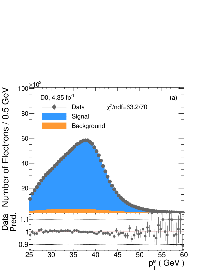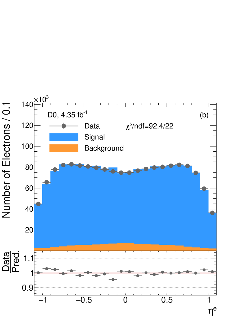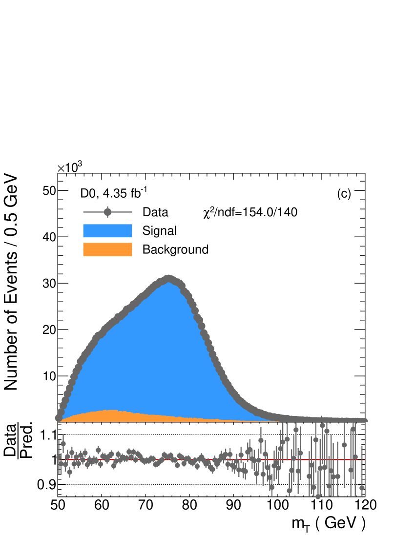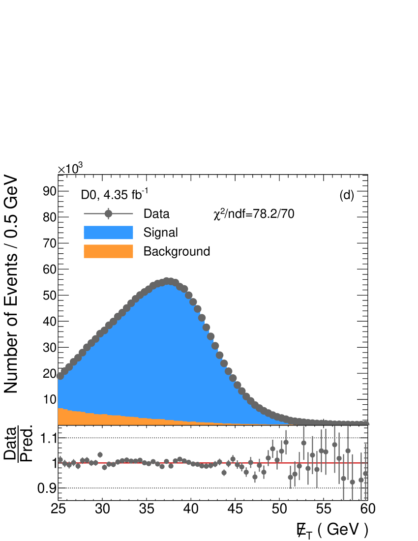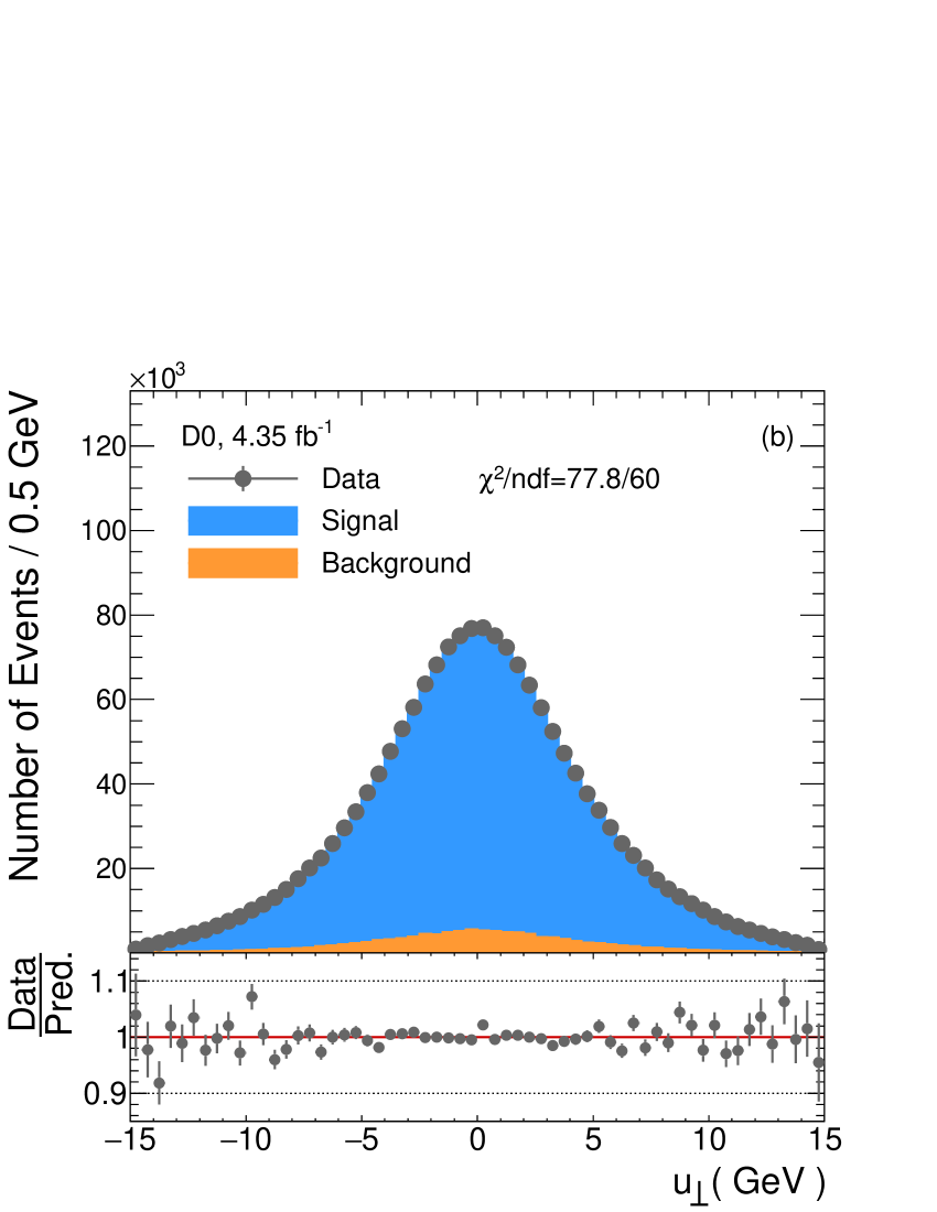The fractions of these backgrounds relative to the signal are $1.08\%\pm 0.02$ % for $Z\to ee$ , $1.02\%\pm 0.06$ % for multijet events, and $1.668\%\pm 0.004$ % for $W\to\tau\nu\to e\nu\nu\nu$ .

Refer to caption — Figure 1: [color online] Kinematic distributions for (a) $p_{T}^{e}$ , (b) $\eta^{e}$ , (c) $m_{T}$ , (d) ${/\kern-6.99997ptE}_{T}$ . The data are compared to the PMCS plus background prediction in the upper panel, and the ratio of the data to the PMCS plus background prediction is shown in the lower panels. Only the statistical uncertainty is included.

Several kinematic distributions of the signal predictions of PMCS together with the expected background contributions taken from Ref. D0NewW are compared to data for $W$ boson candidate events in Figs. 1 and 2. The lepton transverse momentum, the lepton rapidity, the transverse mass, and the missing transverse energy shown in Fig. 1, are not directly sensitive to $p_{T}^{W}$ and therefore probe the general consistency of the simulation. To test the hadronic recoil modeling, we show in Fig. 2 the data and MC comparisons for the components of the hadronic recoil parallel to ( $u_{\parallel}$ ) and perpendicular to ( $u_{\perp}$ ) the direction of the electron. For all distributions in Figs. 1 and 2, the simulation is found to agree with the data.

VI. ANALYSIS STRATEGY

The comparison of several $p_{T}^{W}$ models to data can be achieved either by comparing unfolded data directly with the predictions or by comparing predictions after accounting for detector response and resolution effects with background-subtracted data. Here folding refers to the modification of the model due to detector effects so as to compare directly to the reconstructed level data. Unfolding is the reverse transformation of the data to the particle level for comparison with the theoretical model. The limited $u_{T}$ detector resolution implies a large sensitivity to statistical fluctuations when unfolding, which have to be mitigated by a regularization scheme that increases the possible bias and thus the overall uncertainty. We therefore choose to perform the comparisons with the theory prediction at the reconstruction level.

The folding of the different theory predictions with the D0 detector response is based on the PMCS framework. In the first step, the baseline model of the $W$ boson production is reweighted in two dimensions, $p_{T}^{W}$ and $y^{W}$ , to an alternative theory prediction to be tested. Here $y^{W}$ is the rapidity of the $W$ boson, which is highly correlated with $p_{T}^{W}$ . In the second step, the reweighted theory prediction is used as input for the PMCS framework, resulting in detector level distributions of all relevant observables. In the third step, the uncertainties due to limited MC statistics, the hadronic recoil calibration, the electron identification and reconstruction efficiencies, as well as the electron energy response are estimated for each theory prediction by varying all relevant detector response parameters of the PMCS framework within their uncertainties. Uncertainties due to limited MC statistics, the uncertainties due to the electron identification and reconstruction efficiencies as well as the electron energy response are found to be negligible for the $u_{T}$ distribution. The hadronic recoil calibration is modeled by five calibration parameters D0NewW . These five parameters are divided into two groups, one containing three parameters for the response of $u_{T}$ and the other containing two parameters for the resolution of $u_{T}$ . Only the parameters in the same group are considered to be correlated. Given the correlation matrices of these two groups of parameters, these five parameters are transformed into another five uncorrelated parameters by a linear combination. Each component of the hadronic recoil uncertainty is estimated by varying one of the five uncorrelated parameters with its uncertainty. The combined hadronic recoil uncertainty is calculated by adding in quadrature the individual components in each $u_{T}$ bin. The uncertainty from each component is considered to be bin-by-bin correlated, and the uncertainties from different components are assumed to be uncorrelated.

The uncertainties on the measured $u_{T}$ distribution of the background-subtracted data are the statistical uncertainty, which is treated as bin-to-bin uncorrelated, and the uncertainty due to the background, which is significantly smaller than the statistical uncertainty. The background uncertainty is obtained by varying the overall number of events from each background contribution independently within its uncertainty, so this uncertainty should be considered to be bin-by-bin correlated. Because the uncertainties are small, the effects of these correlations are found to be negligible.

The resulting fractions of events in the $u_{T}$ bins with boundaries $[0,2,5,8,11,15]~{}\text{GeV}$ are summarized in Table 1 for the background-subtracted data along with the combined statistical and systematic uncertainties.

Table 1: The fraction of

W

boson events in bins of

u_{T}

for the background-subtracted data. The combined statistical and systematic uncertainties are shown.

$u_{T}$ bin	0–2 GeV	2–5 GeV	5–8 GeV	8–11 GeV	11–15 GeV
Fraction of events in the $u_{T}$ bin	0.1181	0.3603	0.2738	0.1515	0.0963
Total uncertainty	0.0003	0.0005	0.0005	0.0004	0.0003

VIII. RESULTS AND COMPARISON TO THEORY

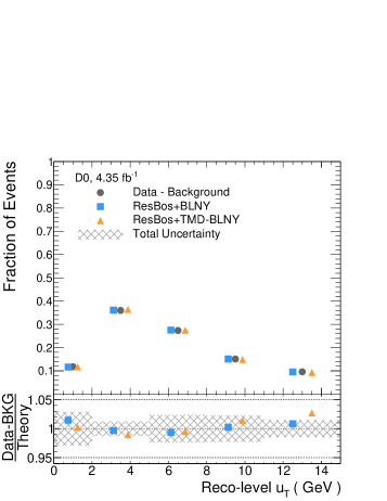
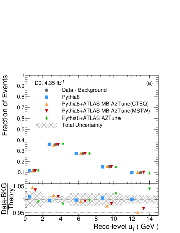
At the reconstruction level, the $u_{T}$ distribution of the background-subtracted data is compared to the predictions of resbos and pythia listed in Section III. The predictions are normalized to the background-subtracted data with $u_{T}<15$ GeV. The data are compared to resbos predictions based on two different non-perturbative functions, BLNY and TMD-BLNY in Fig. 3. Figure 4 shows comparisons with pythia predictions using the different tunes provided by several collaborations. All five $u_{T}$ bins are considered in the $\chi^{2}$ calculation. The uncertainties due to the resummation calculation of resbos and the tune of pythia are not considered in the comparison and the $\chi^{2}$ calculation, and the uncertainty due to the PDF set is negligible. Since both the data and the prediction are normalized to unity, the number of degrees of freedom is 4. The resulting $\chi^{2}/$ ndf values for all models and the corresponding significances in the Gaussian approximation are summarized in Table 2. From this comparison, pythia 8+ATLAS MB A2Tune+CTEQ6L1 is excluded with a $p$ -value equal to $5.84\times 10^{-10}$ and pythia 8+CMS UE Tune CUETP8S1-CTEQ6L1+CTEQ6L1 is excluded with a $p$ -value equal to $4.23\times 10^{-7}$ . All the other pythia 8 predictions except the default, pythia 8+CT14HERA2NNLO, are disfavored. The model based on resbos+BLNY agrees with the data.

Table 2: Chi-squared per degree of freedom and the corresponding

p

-value for the reconstructed-level comparison. Significance is the number of standard deviations in the Gaussian approximation for the difference between each model and the background-subtracted data. Since the distributions are normalized to unity before the comparison, the number of degrees of freedom is 4.

Generator/Model	$\chi^{2}/$ ndf	$p$ -value	Signif.
resbos (Version CP 020811)+BLNY+CTEQ6.6	0.49	$7.41\times 10^{-1}$	0.33
resbos (Version CP 112216)+TMD-BLNY+CT14HERA2NNLO	3.13	$1.39\times 10^{-2}$	2.46
pythia 8+CT14HERA2NNLO	0.32	$8.63\times 10^{-1}$	0.17
pythia 8+ATLAS MB A2Tune+CTEQ6L1	12.25	$5.84\times 10^{-10}$	6.19
pythia 8+ATLAS MB A2Tune+MSTW2008LO	6.17	$5.83\times 10^{-5}$	4.02
pythia 8+ATLAS AZTune+CT14HERA2NNLO	6.61	$2.60\times 10^{-5}$	4.21
pythia 8+Tune2C+CTEQ6L1	7.66	$3.61\times 10^{-6}$	4.63
pythia 8+Tune2M+MRSTLO	7.32	$6.89\times 10^{-6}$	4.50
pythia 8+CMS UE Tune CUETP8S1-CTEQ6L1+CTEQ6L1	8.80	$4.23\times 10^{-7}$	5.06

IX. CONCLUSION

We report a study of the normalized transverse momentum distribution of $W$ bosons produced in $p\bar{p}$ collisions at a center of mass energy of 1.96 TeV, using 4.35 fb^-1 of data collected by the D0 collaboration at the Fermilab Tevatron collider. The $u_{T}$ distribution of the data is compared to those from several theory predictions at the reconstruction level. From these comparisons, pythia 8+ATLAS MB A2Tune+CTEQ6L1 and pythia 8+CMS UE Tune CUETP8S1- CTEQ6L1+CTEQ6L1 are excluded. All the other pythia 8 predictions except the default, pythia 8+CT14HERA2NNLO, are disfavored. Both models based on resbos give satisfactory fits to the data. The precision is limited by the uncertainty due to the hadronic recoil calibration.

In the appendix, we describe a procedure by which theoretical models for the $p_{T}$ distribution of $W$ boson production beyond those considered in this paper can be quantitatively compared to the D0 data.

This study is the first inclusive $p_{T}^{W}$ analysis using Tevatron Run II data. Our data are binned sufficiently finely in $p_{T}^{W}$ to resolve the peak in the cross section, unlike the previous measurements at the LHC. In comparison to measurements by LHC experiments, which involve sea quarks, this work provides additional information for evaluating resummation calculations of transverse momentum of $W$ bosons when the production is dominated by valence quarks.

ACKNOWLEDGEMENTS

This document was prepared by the D0 collaboration using the resources of the Fermi National Accelerator Laboratory (Fermilab), a U.S. Department of Energy, Office of Science, HEP User Facility. Fermilab is managed by Fermi Research Alliance, LLC (FRA), acting under Contract No. DE-AC02-07CH11359.

We thank the staffs at Fermilab and collaborating institutions, and acknowledge support from the Department of Energy and National Science Foundation (United States of America); Alternative Energies and Atomic Energy Commission and National Center for Scientific Research/National Institute of Nuclear and Particle Physics (France); Ministry of Education and Science of the Russian Federation, National Research Center “Kurchatov Institute” of the Russian Federation, and Russian Foundation for Basic Research (Russia); National Council for the Development of Science and Technology and Carlos Chagas Filho Foundation for the Support of Research in the State of Rio de Janeiro (Brazil); Department of Atomic Energy and Department of Science and Technology (India); Administrative Department of Science, Technology and Innovation (Colombia); National Council of Science and Technology (Mexico); National Research Foundation of Korea (Korea); Foundation for Fundamental Research on Matter (The Netherlands); Science and Technology Facilities Council and The Royal Society (United Kingdom); Ministry of Education, Youth and Sports (Czech Republic); Bundesministerium für Bildung und Forschung (Federal Ministry of Education and Research) and Deutsche Forschungsgemeinschaft (German Research Foundation) (Germany); Science Foundation Ireland (Ireland); Swedish Research Council (Sweden); China Academy of Sciences and National Natural Science Foundation of China (China); and Ministry of Education and Science of Ukraine (Ukraine).

APPENDIX. DETECTOR RESPONSE FOR FUTURE COMPARISONS

In order to compare additional model predictions to the measured data, some previous measurements DZeroWPt2 ; ATLASWPt ; CMSPt have been unfolded to the particle level. However, in this study, instead of providing the unfolded particle level $p_{T}^{W}$ distribution, a fast folding procedure is introduced for two reasons: first, no new piece of information would be added by the unfolding procedure so the precision on the particle level would not be better than that on the reconstruction level. Due to the systematic uncertainty from the MC modeling or the regularization which would be introduced by an unfolding method, the precision of the unfolded particle level distribution would be reduced. This reduction would be greater when the resolution of the distribution is worse, and it would be smaller when the bin width is enlarged. But when the bin width is too large, the rise and hence the shape of the spectrum cannot be resolved. Second, it is hard to estimate the bin-by-bin correlation of the uncertainty due to the MC modeling or the regularization properly, since the definitions of these uncertainties are often arbitrary. Therefore, the folding method provided gives a more precise and reliable means of comparison than would an unfolded result.

This fast folding procedure has to be applied on $p_{T}^{W}$ spectra within the fiducial region defined by an electron with $p_{T}^{e}>25$ GeV and $|\eta^{e}|<1.05$ , a $W$ boson with $50<m_{T}<200$ GeV and a neutrino with $p_{T}^{\nu}>25$ GeV. The numbers of events in $p_{T}^{W}$ bins with boundaries $[0,2,5,8,11,15,600]~{}\text{GeV}$ are the input to this folding procedure.

In the first step, the spectrum has to be corrected for the detector efficiency in each $p_{T}^{W}$ bin, via

X_{i}^{{\mathrm{corr}}}={\cal{E}}_{i}X_{i}.

Here $X_{i}$ is the number of events in bin $i$ of the $p_{T}^{W}$ distribution within the fiducial region, ${\cal{E}}_{i}$ is the detector efficiency summarized in Table 3 and $X_{i}^{{\mathrm{corr}}}$ is the number of efficiency-corrected events on the particle level in bin $i$ . Even though most of the events with $p_{T}^{W}>100$ GeV will not satisfy $u_{T}<15$ GeV after the PMCS simulation, we still chose $600$ GeV as the upper edge of the last $p_{T}^{W}$ bin. This is because the efficiency correction in the last $p_{T}^{W}$ bin is directly related to this choice, and the upper edge of the last $p_{T}^{W}$ bin should be kept the same as the value used when deriving those efficiency correction factors.

Table 3: The efficiency correction

{\cal{E}}(p_{T}^{W})

in each

p_{T}^{W}

bin. The efficiency correction is the probability to pass theion selection for the events that pass the particle level selection.

$p_{T}^{W}$ bin	0–2 GeV	2–5 GeV	5–8 GeV	8–11 GeV	11–15 GeV	15–600 GeV
${\cal{E}}(p_{T}^{W})$	0.2330	0.2367	0.2387	0.2396	0.2385	0.2332

The second step accounts for the mapping from $p_{T}^{W}$ to $u_{T}$ using the response matrix $R_{ij}$ via

N_{i}=\sum_{j=1}^{6}R_{ij}X_{j}^{{\mathrm{corr}}},

where $N_{i}$ is the resulting number of events of the reconstruction level in bin $i$ and $R_{ij}$ is a $5\times 6$ matrix. The response matrix is obtained for the signal sample using the PMCS framework and it is summarized in Table 4.

Table 4: Detector response matrix. The number in each cell is the probability for the events in one

p_{T}^{W}

bin to be reconstructed into different

u_{T}

bins.

$p_{T}^{W}$ bin	0–2 GeV	2–5 GeV	5–8 GeV	8–11 GeV	11–15 GeV	15–600 GeV
$0<u_{T}<2$ GeV	0.1784	0.1696	0.1212	0.0745	0.0372	0.0069
$2<u_{T}<5$ GeV	0.4636	0.4588	0.4109	0.3163	0.1974	0.0452
$5<u_{T}<8$ GeV	0.2452	0.2524	0.2966	0.3331	0.3146	0.1121
$8<u_{T}<11$ GeV	0.0806	0.0863	0.1193	0.1810	0.2495	0.1637
$11<u_{T}<15$ GeV	0.0269	0.0270	0.0428	0.0775	0.1550	0.2210

In the third step, after the application of the response matrix, the resulting spectrum has to be corrected for events which would have passed the reconstruction level cuts but not the particle level selection, via

N_{i}^{{\mathrm{corr}}}=\frac{N_{i}}{F_{i}}.

Here $F_{i}$ is the fiducial correction factor in $u_{T}$ bin $i$ and $N_{i}^{{\mathrm{corr}}}$ is the number of fiducial-corrected events on the reconstruction level in bin $i$ . The corresponding fiducial correction factors are derived from the nominal signal sample using PMCS and are summarized in Table 5.

Table 5: The fiducial correction

F(u_{T})

in each

u_{T}

bin. The fiducial correction is the probability to pass the particle level selection for the events that pass theion selection.

$u_{T}$ bin	0–2 GeV	2–5 GeV	5–8 GeV	8–11 GeV	11–15 GeV
$F(u_{T})$	0.8624	0.8689	0.8797	0.8812	0.9036

Finally, in order to get the shape of the distribution, the folded $u_{T}$ distribution is normalized to unity. The fraction of the events in each $u_{T}$ bin, ${\cal{N}}_{i}$ , is calculated via the following formula:

{\cal{N}}_{i}=\frac{N_{i}^{{\mathrm{corr}}}}{\sum_{j=1}^{5}N_{j}^{{\mathrm{corr}}}}

This normalized $u_{T}$ distribution is the folded result, which can be compared to the background-subtracted data directly.

This fast folding procedure is demonstrated to give reconstruction level distributions consistent with those provided by PMCS for the models studied in this paper. Both the efficiency correction and the response matrix are applied directly to the $p_{T}^{W}$ distribution and hence no model assumptions are made. However, the fiducial correction could depend on details of the theoretical model used. We have tested this possibility using two toy production models which differ from our baseline model by either shifting the peak in the $p_{T}^{W}$ distribution by 20% or by broadening the peak by about 20%. In these cases, the $u_{T}$ distributions resulting from the fast folding procedure differed negligibly from those using PMCS .

In order to calculate the chi-square value for the difference between the folded theory prediction and the background-subtracted data, the uncertainty of the folded distribution in each $u_{T}$ bin and the bin-by-bin correlation matrix are also needed. In this fast folding procedure, the detector response is represented by two corrections, the fiducial correction and the efficiency correction, and one detector response matrix. Since the systematic uncertainty is estimated from the difference in the normalized $u_{T}$ distribution between the nominal response and the systematic variation, the uncertainty and the correlation matrix are model dependent, which is why the folding inputs for all of the systematic variations must be provided.

The uncertainty on the $u_{T}$ distribution consists of three independent parts: the uncertainty due to the MC statistics, the uncertainty due to the hadronic recoil calibration, and the uncertainty due to the electron identification and reconstruction efficiencies and the electron energy response. The dominant uncertainty is the one due to the hadronic recoil. The uncertainty due to the MC statistics is directly provided in Table 6, which is considered to be bin-by-bin uncorrelated.

Table 6: The systematic uncertainty due to the MC statistics in each

u_{T}

bin of the folded result.

$u_{T}$ bin	0–2 GeV	2–5 GeV	5–8 GeV	8–11 GeV	11–15 GeV
Uncertainty due to the MC statistics in the folded $u_{T}$ distribution	0.0005	0.0007	0.0006	0.0005	0.0004

Table 7: The efficiency correction

{\cal{E}}(p_{T}^{W})

in each

p_{T}^{W}

bin from eleven systematic variations. The efficiency correction is the probability to pass the reconstruction level selection for the events that pass the particle level selection. The first ten systematic variations are for the uncertainty due to the hadronic recoil and the last one is for the uncertainty due to the electron energy response.

$p_{T}^{W}$ bin	0–2 GeV	2–5 GeV	5–8 GeV	8–11 GeV	11–15 GeV	15–600 GeV
Systematic Variation No. 1	0.2348	0.2374	0.2377	0.2405	0.2392	0.2332
Systematic Variation No. 2	0.2345	0.2370	0.2392	0.2377	0.2382	0.2334
Systematic Variation No. 3	0.2336	0.2374	0.2388	0.2377	0.2378	0.2317
Systematic Variation No. 4	0.2335	0.2369	0.2394	0.2385	0.2379	0.2329
Systematic Variation No. 5	0.2323	0.2365	0.2392	0.2385	0.2393	0.2326
Systematic Variation No. 6	0.2337	0.2355	0.2390	0.2408	0.2387	0.2321
Systematic Variation No. 7	0.2342	0.2373	0.2384	0.2386	0.2390	0.2318
Systematic Variation No. 8	0.2328	0.2362	0.2384	0.2386	0.2390	0.2322
Systematic Variation No. 9	0.2360	0.2369	0.2382	0.2398	0.2376	0.2323
Systematic Variation No. 10	0.2327	0.2371	0.2387	0.2390	0.2387	0.2328
Systematic Variation No. 11	0.2343	0.2370	0.2379	0.2399	0.2374	0.2315

The other two parts of the uncertainty should be estimated with systematic variations. There are eleven systematic variations provided in total, ten for the uncertainty due to the hadronic recoil calibration and one for the uncertainty due to the efficiency and the energy response of the electron. The hadronic recoil response and resolution are characterized by the five uncorrelated parameters discussed in Section VI. The uncertainties due to positive and negative changes in these parameters differ, so we must evaluate both signs of parameter change, thus giving the first ten variations. The eleventh systematic variation is derived with the parameter $\alpha$ , which is mentioned in Sec. IV, changed by its uncertainty. This is an overestimation of the uncertainty due to the strong anti-correlation between $\alpha$ and $\beta$ . The folding inputs of these eleven systematic variations are provided in Tables 7, 8 and 9. The uncertainties from different variations are considered to be uncorrelated and the uncertainty from each variation is considered to be bin-by-bin correlated. The bin-by-bin covariance matrix of systematic variation $k$ is defined as $\Sigma^{(k)}$ , whose element is calculated via

\Sigma^{(k)}_{ij}=({\cal{N}}_{i}-{\cal{N}}_{i}^{(k)})\times({\cal{N}}_{j}-{\cal{N}}_{j}^{(k)}).

Here ${\cal{N}}_{i}^{(k)}$ is the folded result from systematic variation $k$ . The covariance matrix of the uncertainty due to the hadronic recoil calibration are calcualted by the average of the covariance matrices from the positive and negative changes. The covariance matrix of the total systematic uncertainty, $\Sigma^{{\mathrm{(Syst.)}}}$ , is calculated as the sum of the covariance matrix of the uncertainty due to the hadronic recoil calibration and that of the uncertainty due to the efficiency and the energy response of the electron, via

\Sigma^{{\mathrm{(Syst.)}}}=\frac{\sum_{k=1}^{10}\Sigma^{(k)}}{2}+\Sigma^{(11)}.

The total uncertainty of the folded result is the combination of the statistical uncertainty and the total systematic uncertainty. The total covariance matrix used in the $\chi^{2}$ calculation, $\Sigma^{{\mathrm{(Total)}}}$ , is the sum of the covariance matrix of the systematic uncertainty and the statistical uncertainties due to both data and MC statistics, $\Sigma^{{\mathrm{(Data~{}stat.)}}}$ and $\Sigma^{{\mathrm{(MC~{}stat.)}}}$ , via

\Sigma^{{\mathrm{(Total)}}}=\Sigma^{{\mathrm{(Data~{}stat.)}}}+\Sigma^{{\mathrm{(MC~{}stat.)}}}+\Sigma^{{\mathrm{(Syst.)}}}.

Here $\Sigma^{{\mathrm{(Data~{}stat.)}}}$ is a diagonal matrix constructed with the total uncertainty provided in Table 1 and $\Sigma^{{\mathrm{(MC~{}stat.)}}}$ is also a diagonal matrix constructed with the uncertainty summarized in Table 6.

Table 8: Detector response matrices for the eleven systematic variations. The numbers in each cell are the probability for the events in one

p_{T}^{W}

bin to be reconstructed into different

u_{T}

bins. The first ten systematic variations are for the uncertainty due to the hadronic recoil and the last one is for the uncertainty due to the electron energy response.

Systematic Variation No. 1
$p_{T}^{W}$ bin	0–2 GeV	2–5 GeV	5–8 GeV	8–11 GeV	11–15 GeV	15–600 GeV
$0<u_{T}<2$	0.1876	0.1738	0.1196	0.0715	0.0363	0.0071
$2<u_{T}<5$	0.4642	0.4588	0.4109	0.3120	0.2022	0.0456
$5<u_{T}<8$	0.2382	0.2503	0.2938	0.3388	0.3107	0.1112
$8<u_{T}<11$	0.0777	0.0840	0.1227	0.1822	0.2535	0.1644
$11<u_{T}<15$	0.0272	0.0275	0.0439	0.0780	0.1503	0.2216
Systematic Variation No. 2
$p_{T}^{W}$ bin	0–2 GeV	2–5 GeV	5–8 GeV	8–11 GeV	11–15 GeV	15–600 GeV
$0<u_{T}<2$	0.1754	0.1669	0.1193	0.0720	0.0356	0.0070
$2<u_{T}<5$	0.4665	0.4607	0.4091	0.3144	0.2009	0.0457
$5<u_{T}<8$	0.2410	0.2506	0.2957	0.3323	0.3113	0.1137
$8<u_{T}<11$	0.0834	0.0880	0.1231	0.1838	0.2511	0.1667
$11<u_{T}<15$	0.0280	0.0281	0.0437	0.0788	0.1532	0.2209
Systematic Variation No. 3
$p_{T}^{W}$ bin	0–2 GeV	2–5 GeV	5–8 GeV	8–11 GeV	11–15 GeV	15–600 GeV
$0<u_{T}<2$	0.1776	0.1702	0.1200	0.0698	0.0340	0.0067
$2<u_{T}<5$	0.4647	0.4618	0.4098	0.3203	0.1988	0.0442
$5<u_{T}<8$	0.2393	0.2496	0.2967	0.3359	0.3078	0.1121
$8<u_{T}<11$	0.0850	0.0852	0.1222	0.1802	0.2584	0.1630
$11<u_{T}<15$	0.0273	0.0275	0.0428	0.0762	0.1542	0.2245
Systematic Variation No. 4
$p_{T}^{W}$ bin	0–2 GeV	2–5 GeV	5–8 GeV	8–11 GeV	11–15 GeV	15–600 GeV
$0<u_{T}<2$	0.1815	0.1744	0.1215	0.0730	0.0366	0.0068
$2<u_{T}<5$	0.4612	0.4577	0.4110	0.3157	0.2022	0.0467
$5<u_{T}<8$	0.2440	0.2505	0.2941	0.3311	0.3114	0.1126
$8<u_{T}<11$	0.0811	0.0842	0.1209	0.1817	0.2509	0.1641
$11<u_{T}<15$	0.0263	0.0279	0.0438	0.0799	0.1504	0.2199
Systematic Variation No. 5
$p_{T}^{W}$ bin	0–2 GeV	2–5 GeV	5–8 GeV	8–11 GeV	11–15 GeV	15–600 GeV
$0<u_{T}<2$	0.1808	0.1697	0.1199	0.0707	0.0355	0.0067
$2<u_{T}<5$	0.4623	0.4617	0.4129	0.3213	0.1973	0.0443
$5<u_{T}<8$	0.2424	0.2498	0.2940	0.3354	0.3130	0.1121
$8<u_{T}<11$	0.0818	0.0857	0.1212	0.1792	0.2526	0.1676
$11<u_{T}<15$	0.0274	0.0277	0.0422	0.0760	0.1561	0.2229
Systematic Variation No. 6
$p_{T}^{W}$ bin	0–2 GeV	2–5 GeV	5–8 GeV	8–11 GeV	11–15 GeV	15–600 GeV
$0<u_{T}<2$	0.1740	0.1716	0.1241	0.0739	0.0364	0.0066
$2<u_{T}<5$	0.4625	0.4609	0.4116	0.3207	0.2011	0.0462
$5<u_{T}<8$	0.2446	0.2489	0.2917	0.3303	0.3145	0.1113
$8<u_{T}<11$	0.0857	0.08433	0.1210	0.1817	0.246	0.1649
$11<u_{T}<15$	0.0280	0.0287	0.0429	0.0758	0.1537	0.2216
Systematic Variation No. 7
$p_{T}^{W}$ bin	0–2 GeV	2–5 GeV	5–8 GeV	8–11 GeV	11–15 GeV	15–600 GeV
$0<u_{T}<2$	0.1803	0.1725	0.1233	0.0711	0.0352	0.0071
$2<u_{T}<5$	0.4648	0.4612	0.4121	0.3197	0.2025	0.0454
$5<u_{T}<8$	0.2423	0.2507	0.2934	0.3320	0.3110	0.1092
$8<u_{T}<11$	0.0810	0.0832	0.1188	0.1826	0.2545	0.1643
$11<u_{T}<15$	0.0263	0.0268	0.0434	0.0768	0.1493	0.2239
Systematic Variation No. 8
$p_{T}^{W}$ bin	0–2 GeV	2–5 GeV	5–8 GeV	8–11 GeV	11–15 GeV	15–600 GeV
$0<u_{T}<2$	0.1805	0.1722	0.1218	0.0705	0.0379	0.0070
$2<u_{T}<5$	0.4648	0.4602	0.4123	0.3172	0.2052	0.0466
$5<u_{T}<8$	0.2399	0.2481	0.2927	0.3379	0.3114	0.1137
$8<u_{T}<11$	0.0826	0.0863	0.1215	0.1805	0.2477	0.1653
$11<u_{T}<15$	0.0266	0.0278	0.0432	0.0764	0.1517	0.2235
Systematic Variation No. 9
$p_{T}^{W}$ bin	0–2 GeV	2–5 GeV	5–8 GeV	8–11 GeV	11–15 GeV	15–600 GeV
$0<u_{T}<2$	0.1774	0.1709	0.1241	0.0717	0.0348	0.0064
$2<u_{T}<5$	0.4618	0.4563	0.4077	0.3188	0.1980	0.0445
$5<u_{T}<8$	0.2444	0.2525	0.2958	0.3335	0.3138	0.1116
$8<u_{T}<11$	0.0833	0.0866	0.1216	0.1798	0.2512	0.1657
$11<u_{T}<15$	0.0275	0.0278	0.0417	0.0782	0.1542	0.2226
Systematic Variation No. 10
$p_{T}^{W}$ bin	0–2 GeV	2–5 GeV	5–8 GeV	8–11 GeV	11–15 GeV	15–600 GeV
$0<u_{T}<2$	0.1826	0.1720	0.1198	0.0708	0.0370	0.0073
$2<u_{T}<5$	0.4598	0.4584	0.4100	0.3168	0.2026	0.0469
$5<u_{T}<8$	0.2420	0.2483	0.2988	0.3346	0.3091	0.1120
$8<u_{T}<11$	0.0827	0.0876	0.1195	0.1819	0.2494	0.1628
$11<u_{T}<15$	0.0273	0.0278	0.0430	0.0774	0.1546	0.2204
Systematic Variation No. 11
$p_{T}^{W}$ bin	0–2 GeV	2–5 GeV	5–8 GeV	8–11 GeV	11–15 GeV	15–600 GeV
$0<u_{T}<2$	0.1790	0.1707	0.1192	0.0716	0.0349	0.0072
$2<u_{T}<5$	0.4624	0.4629	0.4102	0.3176	0.2030	0.0472
$5<u_{T}<8$	0.2436	0.2484	0.2967	0.3341	0.3116	0.1108
$8<u_{T}<11$	0.0839	0.0853	0.1223	0.1830	0.2483	0.1653
$11<u_{T}<15$	0.0259	0.0271	0.0431	0.0763	0.1561	0.2229

Table 9: The fiducial correction

F(u_{T})

in each

u_{T}

bin for the eleven systematic variations. The fiducial correction is the probability to pass the particle level selection for the events that pass theion selection. The first ten systematic variations are for the uncertainty due to the hadronic recoil and the last one is for the uncertainty due to the electron energy response.

$u_{T}$ bin	0–2 GeV	2–5 GeV	5–8 GeV	8–11 GeV	11–15 GeV
Systematic Variation No. 1	0.8639	0.8705	0.8778	0.8814	0.9011
Systematic Variation No. 2	0.8629	0.8686	0.8787	0.8817	0.9033
Systematic Variation No. 3	0.8612	0.8703	0.8796	0.8824	0.9003
Systematic Variation No. 4	0.8637	0.8673	0.8789	0.8819	0.9002
Systematic Variation No. 5	0.8637	0.8690	0.8803	0.8795	0.9037
Systematic Variation No. 6	0.8638	0.8686	0.8779	0.8799	0.9020
Systematic Variation No. 7	0.8634	0.8691	0.8805	0.8830	0.8996
Systematic Variation No. 8	0.8651	0.8695	0.8795	0.8821	0.8992
Systematic Variation No. 9	0.8664	0.8691	0.8800	0.8819	0.9004
Systematic Variation No. 10	0.8630	0.8691	0.8786	0.8808	0.9007
Systematic Variation No. 11	0.8615	0.8700	0.8798	0.8842	0.9004

As a validation, the $\chi^{2}$ values calculated from the fast folding approach are compared to those provided in Table 2. The background-subtracted data is fluctuated with the statistical uncertainty from the data in order to estimate the impact on $\chi^{2}/$ ndf from the data statistics. The difference between the chi-square values calculated from the PMCS simulation and that calculated from the fast folding is negligible compared to the impact of the statistical fluctuation of the data, hence validating this approach.

References

(1) M. Schott and M. Dunford, “Review of single vector boson production in pp collisions at $\sqrt{s}$ =7-TeV”, Eur. Phys. J. C 74, 2916 (2014).
(2) J. Collins et al.,“Transverse Momentum Distribution in Drell-Yan Pair and $W$ and $Z$ Boson Production”, Nucl. Phys. B250, 199 (1985).
(3) C. Balazs and C. P. Yuan, “Soft gluon effects on lepton pairs at hadron colliders”, Phys. Rev. D 56, 5558 (1997).
(4) T. Becher and M. Neubert, “Drell-Yan Production at Small $q_{T}$ , Transverse Parton Distributions and the Collinear Anomaly”, Eur. Phys. J. C 71, 1665 (2011).
(5) S. Catani et al., “Vector boson production at hadron colliders: transverse-momentum resummation and leptonic decay”, J. High Energy Phys. 12, 47 (2015).
(6) M. A. Ebert and F. J. Tackmann, “Resummation of Transverse Momentum Distributions in Distribution Space”, J. High Energy Phys. 02, 110 (2017).
(7) W. Bizon et al., “Momentum-space resummation for transverse observables and the Higgs p_⟂ at N³LL+NNLO”, J. High Energy Phys. 02, 108 (2018).
(8) J .Bellm et al., “Herwig 7.0/Herwig++ 3.0 release note”, Eur. Phys. J. C 76, 196 (2016).
(9) T. Sjöstrand et al., “An Introduction to PYTHIA 8.2”, Comput. Phys. Commun. 191, 159 (2015).
(10) E. Bothmann et al., “Event Generation with Sherpa 2.2”, SciPost Phys. 7, 034 (2019).
(11) G. A. Ladinsky and C. P. Yuan, “The nonperturbative regime in QCD resummation for gauge boson production at hadron colliders”, Phys. Rev. D 50, R4239 (1994).
(12) A. V. Konychev and P. M. Nadolsky, “Universality of the Collins-Soper-Sterman nonperturbative function in gauge boson production”, Phys. Lett. 633B, 710 (2006).
(13) V. M. Abazov et al. (DØ Collaboration), “Measurement of the shape of the boson transverse momentum distribution in $p\bar{p}\to Z/\gamma^{*}\to e^{+}e^{-}+X$ events produced at $\sqrt{s}$ =1.96-TeV”, Phys. Rev. Lett. 100, 102002 (2008).
(14) V. M. Abazov et al. (DØ Collaboration), “Measurement of the Normalized $Z/\gamma^{*}->\mu^{+}\mu^{-}$ Transverse Momentum Distribution in $p\bar{p}$ Collisions at $\sqrt{s}=1.96$ TeV”, Phys. Lett. 693B, 522 (2010).
(15) V. M. Abazov et al. (DØ Collaboration), “Precise Study of the $Z/\gamma^{*}$ Boson Transverse Momentum Distribution in $p\bar{p}$ Collisions using a Novel Technique”, Phys. Rev. Lett. 106, 122001 (2011).
(16) T. Aaltonen et al. (CDF Collaboration), “Transverse momentum cross section of $e^{+}e^{-}$ pairs in the $Z$ -boson region from $p\bar{p}$ collisions at $\sqrt{s}=1.96$ TeV”, Phys. Rev. D 86, 052010 (2012).
(17) G. Aad et al. (ATLAS Collaboration), “Measurement of the transverse momentum and $\phi^{*}_{\eta}$ distributions of Drell–Yan lepton pairs in proton–proton collisions at $\sqrt{s}=8$ TeV with the ATLAS detector”, Eur. Phys. J. C 76, 1 (2016).
(18) G. Aad et al. (ATLAS Collaboration), “Measurement of the $Z/\gamma^{*}$ boson transverse momentum distribution in $pp$ collisions at $\sqrt{s}$ = 7 TeV with the ATLAS detector”, J. High Energy Phys. 09, 145 (2014).
(19) G. Aad et al. (ATLAS Collaboration), “Measurement of the Transverse Momentum Distribution of $W$ Bosons in $pp$ Collisions at $\sqrt{s}=7$ TeV with the ATLAS Detector”, Phys. Rev. D 85, 012005 (2012).
(20) S. Chatrchyan et al. (CMS Collaboration), “Measurement of the $Z$ boson differential cross section in transverse momentum and rapidity in proton–proton collisions at 8 TeV”, Phys. Lett. B 749, (2015) 187.
(21) S. Chatrchyan et al. (CMS Collaboration), “Measurement of the Rapidity and Transverse Momentum Distributions of $Z$ Bosons in $pp$ Collisions at $\sqrt{s}=7$ TeV”, Phys. Rev. D 85, 032002 (2012).
(22) S. Chatrchyan et al. (CMS Collaboration), “Measurement of the transverse momentum spectra of weak vector bosons produced in proton-proton collisions at $\sqrt{s}=8$ TeV”, J. High Energy Phys. 02, 96 (2017).
(23) V. M. Abazov et al. (DØ Collaboration), “Measurement of the Shape of the Transverse Momentum Distribution of $W$ Bosons Produced in $p\bar{p}$ Collisions at sqrt(s)= 1.8 TeV”, Phys. Rev. Lett. 80, 5498 (1998).
(24) V. M. Abazov et al. (DØ Collaboration), “Differential cross section for $W$ boson production as a function of transverse momentum in proton-antiproton collisions at 1.8 TeV”, Phys. Lett. 513B, 292 (2001).
(25) G. Aad et al. (ATLAS Collaboration), “Measurement of the transverse momentum distribution of $W$ bosons in pp collisions at $\sqrt{(}s)=7$ TeV with the ATLAS detector”, Phys. Rev. D 85, 012005 (2012).
(26) V. M. Abazov et al. (DØ Collaboration), “Measurement of the $W$ Boson Mass with the D0 Detector”, Phys. Rev. Lett. 108, 151804 (2012).
(27) V. M. Abazov et al. (DØ Collaboration), “The Upgraded D0 detector”, Nucl. Instrum. Methods A 565, 463 (2006).
(28) V. M. Abazov et al. (DØ Collaboration), “Measurement of the $W$ boson mass with the D0 detector”, Phys. Rev. D 89, 012005 (2014).
(29) P. Golonka and Z. Was, PHOTOS Monte Carlo: “A Precision tool for QED corrections in $Z$ and $W$ decays”, Eur. Phys. J. C45, 97 (2006).
(30) F. Landry et al., “Tevatron Run-1 $Z$ boson data and Collins-Soper-Sterman resummation formalism”, Phys. Rev. D 67, 073016 (2003).
(31) P. M. Nadolsky et al., “Implications of CTEQ global analysis for collider observables”, Phys. Rev. D 78, 013004 (2008).
(32) M. Guzzi et al., “CTEQ-TEA parton distribution functions with intrinsic charm”, J. High Energy Phys. 02, 059 (2018).
(33) S. Dulat et al., “New parton distribution functions from a global analysis of quantum chromodynamics”, Phys. Rev. D 93, 033006 (2016).
(34) J. Pumplin, et al., “New generation of parton distributions with uncertainties from global QCD analysis”, J. High Energy Phys. 07, 012 (2002).
(35) A, D. Martin et al., “Parton distributions for the LHC”, Eur. Phys. J. C63, 189 (2009).
(36) A. D. Martin et al., “MRST partons generated in a fixed-flavor scheme”, Phys. Lett. 636B, 259 (2006).
(37) P. Sun et al., “Nonperturbative functions for SIDIS and Drell-Yan processes”, Int. J. Mod. Phys. A33, 1841006 (2018).
(38) G. Aad et al. (ATLAS Collaboration), “Summary of ATLAS Pythia 8 tunes”, ATL-PHYS-PUB-2012-003.
(39) R. Corke and T. Sjöstrand, “Interleaved Parton Showers and Tuning Prospects”, J. High Energy Phys. 03, 032 (2011).
(40) S. Chatrchyan et al. (CMS Collaboration), “Event generator tunes obtained from underlying event and multiparton scattering measurements”, Eur. Phys. J. C 76, 155 (2016).
(41) R. Brun and F. Carminati, CERN Program Library Long Writeup W5013, 1993 (unpublished).
(42) J. Alitti et al. (UA2 Collaboration), “An Improved determination of the ratio of $W$ and $Z$ masses at the CERN $\bar{p}p$ collider”, Phys. Lett. 276B, 354 (1992).

Study of the normalized transverse momentum distribution of W𝑊W bosons produced in p​p¯𝑝¯𝑝p\bar{p} collisions at s=1.96𝑠1.96\sqrt{s}=1.96 TeV

Abstract

pacs:

References

Study of the normalized transverse momentum distribution of $W$ bosons produced in $p\bar{p}$ collisions at $\sqrt{s}=1.96$ TeV