The ’t Hooft–Polyakov monopole in the geometric theory of defects

Abstract

The ’t Hooft–Polyakov monopole solution in Yang–Mills theory is given new physical interpretation in the geometric theory of defects. It describes solids with continuous distribution of dislocations and disclinations. The corresponding densities of Burgers and Frank vectors are computed. It means that the ’t Hooft–Polyakov monopole can be seen, probably, in solids.

1 Introduction

Important properties of real crystals such as plasticity, melting, growth, etc., are mainly defined by defects of the crystalline structure which are called dislocations. Moreover, many bodies posses a spin structure. For example, ferromagnets are also characterized by the distribution of magnetic moments described by the unit vector field. This unit vector field may also have defects (singularities) which are called disclinations. Description of dislocations and disclinations in elastic media is a very active field of research for more then one century because of its importance for applications (see, e.g., [1, 2]).

Real solids posses usually a crystalline structure and are often described by models based on this crystalline structure especially at the quantum level. At the same time, many properties of solids can be also described by the elasticity theory in the continuous approximation. Discrete and continuous approaches complement each other, and are both needed for our understanding of nature.

In this paper, we consider only continuous approximation. In this approximation solids without dislocations are described by the displacement vector field within the ordinary elasticity theory. The spin structure of solids without disclinations is described by the unit vector field ($n$-field) satisfying appropriate field equations. In the presence of dislocations and disclinations there as a problem: what variable are to be used? For example, real solids posses many defects, and if we want to use continuous approximation for defect distributions then the displacement vector field and $n$-filed do not exist because they are singular at each point. The geometric theory of defects is aimed to resolve this problem.

The idea of geometric theory of defects is simple. In the continuous approximation, a crystal with a spin structure is considered as elastic media (manifold) with a given metric and affine connection with torsion (the Riemann–Cartan geometry). As usual, elastic deformations of media and distribution of the unit vector field are described by the displacement and rotational angle vector fields. The absence of defects means that displacement and unit vector fields are smooth. If they are not continuous then we say that the media has defects. In general, there are two types of defects: dislocations which are defects of elastic media itself (discontinuity of the displacement vector field) and disclinations corresponding to discontinuities of the unit vector field. If defects are absent, then geometry is trivial: curvature and torsion are zero. In the presence of defects, geometry becomes nontrivial. Dislocations give rise to torsion and disclinations result in nontrivial curvature. The physical meaning of torsion and curvature are surface densities of Burgers [3, 4] and Frank [5] vectors, respectively, [6, 7]. The geometric theory of defects allows one to describe single defects as well as their continuous distribution. For single defects, torsion and curvature are zero everywhere except some points, lines or surfaces where defects are located and where they have singularities. In the case of continuous distribution of dislocations and disclinations, torsion and curvature become nontrivial on the whole media, and instead of the displacement and angular rotation field we use tetrad and ${\mathbb{S}}{\mathbb{O}}(3)$-connection as the independent variables. The advantage is that these variables exist even in the absence of the displacement and unite vector fields.

The history of geometric theory of defects goes back to 1950s [8–11] when dislocations were related to torsion for the first time. The review and earlier references can be found in the book [12].

In the geometric approach to the theory of defects [6, 7, 13], we discuss the model which is different from others in two respects. Firstly, we do not have the displacement and unit vector fields as independent variables because, in general, they are not continuous. Instead, the triad field and ${\mathbb{S}}{\mathbb{O}}(3)$-connection are considered as the only independent variables. If defects are absent, then the triad and ${\mathbb{S}}{\mathbb{O}}(3)$-connection reduce to partial derivatives of the displacement and rotational angle vector fields (pure gauge because torsion and curvature vanish). In this case, the latter can be reconstructed. Secondly, the set of equilibrium equations is different. We proposed the purely geometric set which coincides with that of Euclidean three dimensional gravity with torsion. The nonlinear elasticity equations and principal chiral ${\mathbb{S}}{\mathbb{O}}(3)$-model for the unit vector field enter the model through the elastic and Lorentz gauge conditions [14, 15, 7] which allow us to reconstruct the displacement and unit vector fields in the absence of defects in full agreement with classical models.

When a new model is proposed then one has to show how to obtain previous results within new approach. A number of dislocations were described in the geometric theory of defects and shown to be in agreement with the elasticity theory [7], which corresponds to linear approximation. Therefore the geometric theory of defects does not contradict experimental data in the domain where elasticity theory is valid. At the same time, the geometric theory of defects have also different predictions, for example, for the deformation tensor near the core of wedge dislocation. As far as we know, there is no experimental confirmation or refutation of geometric theory of defects. So, the model is still under theoretical development.

In this paper, we consider the possibility of physical interpretation of the ’t Hooft–Polyakov monopole solution [16, 17] in the geometric theory of defects. The famous ’t Hooft–Polyakov solution in the ${\mathbb{S}}{\mathbb{U}}(2)$ gauge theory interacting with the triplet of scalar fields attracted much interest in physics and mathematics (for review, see, for example, [18, 19]). The solution is static and spherically symmetric. Therefore, it reduces to minimization of three-dimensional Euclidean energy expression which can be regarded as the free energy expression in solid state physics. We consider the ${\mathbb{S}}{\mathbb{U}}(2)$-connection components as the ${\mathbb{S}}{\mathbb{O}}(3)$-connection because their Lie algebras coincide, the triplet of scalar fields being the source of defects. Moreover, we assume that the ${\mathbb{S}}{\mathbb{O}}(3)$ group acts not in the isotopic space but in the tangent space to space manifold ${\mathbb{R}}^{3}$. The metric of the space remains Euclidean. So the ’t Hooft–Polyakov monopole corresponds to Euclidean vielbein and nontrivial ${\mathbb{S}}{\mathbb{O}}(3)$-connection which give rise to nontrivial Riemann–Cartan geometry of space.

So, the ’t Hooft–Polyakov monopole solution has natural interpretation in solid state physics describing elastic media with continuous distribution of disclinations and dislocations. We compute the corresponding densities of Frank and Burgers vectors.

2 Geometric theory of defects

In this section we give short review of the geometric theory of defects and introduce basic geometric notions: triad field and ${\mathbb{S}}{\mathbb{O}}(3)$-connection. More details can be found in [7].

We consider a three dimensional continuous media described by a topologically trivial Riemann–Cartan manifold. We use triad field $e_{\mu}{}^{i}$ and ${\mathbb{S}}{\mathbb{O}}(3)$-connection $\omega_{\mu}{}^{ij}=-\omega_{\mu}{}^{ji}$, where Greek letters $\mu=1,2,3$ and Latin ones $i,j=1,2,3$ denote world and tangent indices, respectively, as basic independent variables. We assume that metric $g_{\mu\nu}:=e_{\mu}{}^{i}e_{\nu}{}^{j}\delta_{ij}=\delta_{\mu\nu}$ is an ordinary flat Euclidean metric, but connection is nontrivial and may have singularities on some points, lines, or surfaces.

The simplest and most widespread examples of linear dislocations are shown in Fig. 1 (see, e.g., [1, 2]). They are produced as follows. We cut the medium along the half-plane $x^{2}=0$, $x^{1}>0$, move the upper part of the medium located over the cut $x^{2}>0$, $x^{1}>0$ by the vector $\boldsymbol{b}$ towards the dislocation axis $x^{3}$, and glue the cutting surfaces. The vector $\boldsymbol{b}$ is called the Burgers vector. In a general case, the Burgers vector may not be constant on the cut. For the edge dislocation, it varies from zero to some constant value $\boldsymbol{b}$ as it moves from the dislocation axis. After the gluing, the media comes to the equilibrium state called the edge dislocation, see Fig. 1a. If the Burgers vector is parallel to the dislocation line, it is called the screw dislocation (Fig. 1b).

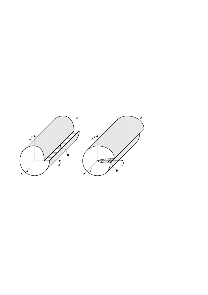
Figure 1: Straight linear dislocations. (a) The edge dislocation. The Burgers vector $\boldsymbol{b}$ is perpendicular to the dislocation line. (b) The screw dislocation. The Burgers vector $\boldsymbol{b}$ is parallel to the dislocation line.

From the topological standpoint, the medium containing several dislocations or even the infinite number of them is still the Euclidean space ${\mathbb{R}}^{3}$. In contrast to the case of elastic deformations, the displacement vector in the presence of dislocations is no longer a smooth function because of the presence of cutting surfaces where it jumps.

The main idea of the geometric approach amounts to the following. To describe single dislocations in the framework of elasticity theory, we must solve equations for the displacement vector with some boundary conditions on the cuts. This is possible for small number of dislocations. But, with an increasing number of dislocations, the boundary conditions become so complicated that the solution of the problem becomes unrealistic. Besides, one and the same dislocation can be created by different cuts which leads to an ambiguity in the displacement vector field. Another shortcoming of this approach is that it cannot be applied to the description of a continuous distribution of dislocations because the displacement vector field does not exist in this case at all because it must have discontinuities at every point. In the geometric approach, we consider the triad field instead of the displacement vector field which is introduced as follows.

Let a point of the medium has Cartesian coordinates $y^{i}$ in the ground equilibrium state. After elastic deformation, this point has the coordinates

$$y^{i}\mapsto x^{i}(y)=y^{i}+u^{i}(x),$$ (1)

where $u^{i}(x)$ is the displacement vector field. We consider its components as functions of final point position $x$.

In a general dislocation-present case, we do not have a preferred Cartesian coordinate system in the equilibrium because there is no symmetry. Therefore, we consider arbitrary global coordinates $x^{\mu}$, $\mu=1,2,3$, in ${\mathbb{R}}^{3}$. We use Greek letters for coordinates allowing arbitrary coordinate changes. Then the Burgers vector for linear dislocation can be expressed as the integral of the displacement vector

$$\oint_{C}dx^{\mu}\partial_{\mu}u^{i}(x)=-\oint_{C}dx^{\mu}\partial_{\mu}y^{i}(x)=-b^{i},$$ (2)

where $C$ is a closed contour surrounding the dislocation axis. This integral is invariant under arbitrary coordinate transformations $x^{\mu}\mapsto x^{\mu^{\prime}}(x)$ and covariant under global ${\mathbb{S}}{\mathbb{O}}(3)$-rotations of $y^{i}$. Here, components of the displacement vector field $u^{i}(x)$ are considered with respect to the orthonormal basis in the tangent space, $u=u^{i}e_{i}$. If components of the displacement vector field are considered with respect to the coordinate basis $u=u^{\mu}\partial_{\mu}$, the invariance of the integral (2) under general coordinate changes is violated.

In the geometric approach, we introduce new independent variable – the triad – instead of partial derivatives $\partial_{\mu}u^{i}$:

$$e_{\mu}{}^{i}(x):=\begin{cases}\partial_{\mu}y^{i},&\text{outside the cut,}\\ {\sf\,lim\,}\partial_{\mu}y^{i},&\text{on the cut.}\end{cases}$$ (3)

The triad is a smooth function on the cut by construction. We note that if the vielbein was simply defined as partial derivatives $\partial_{\mu}y^{i}$, then it would have the $\delta$-function singularity on the cut because functions $y^{i}(x)$ have a jump. The Burgers vector can be expressed through the integral over a surface $S$ having contour $C$ as the boundary:

$$\oint_{C}dx^{\mu}e_{\mu}{}^{i}=\int\!\!\int_{S}dx^{\mu}\wedge dx^{\nu}(\partial_{\mu}e_{\nu}{}^{i}-\partial_{\nu}e_{\mu}{}^{i})=b^{i},$$ (4)

where $dx^{\mu}\wedge dx^{\nu}$ is the surface element. As a consequence of the definition of the vielbein in (3), the integrand is equal to zero everywhere except at the dislocation axis. For the edge dislocation with constant Burgers vector, the integrand has a $\delta$-function singularity at the origin. The criterion for the presence of a dislocation is a violation of the integrability conditions for the system of equations $\partial_{\mu}y^{i}=e_{\mu}{}^{i}$:

$$\partial_{\mu}e_{\nu}{}^{i}-\partial_{\nu}e_{\mu}{}^{i}\neq 0.$$ (5)

If dislocations are absent, then the functions $y^{i}(x)$ exist and define transformation to a Cartesian coordinates frame.

In the geometric theory of defects, the field $e_{\mu}{}^{i}$ is identified with the triad. Next, we compare the integrand in (4) with the expression for the torsion in Cartan variables

$$T_{\mu\nu}{}^{i}:=\partial_{\mu}e_{\nu}{}^{i}-\partial_{\nu}e_{\mu}{}^{j}-e_{\mu}{}^{j}\omega_{\nu j}{}^{i}+e_{\nu}{}^{j}\omega_{\mu j}{}^{i}.$$ (6)

They differ only by terms containing the ${\mathbb{S}}{\mathbb{O}}(3)$-connection $\omega_{\mu j}{}^{i}$. This is the ground for the introduction of the following postulate. In the geometric theory of defects, the Burgers vector corresponding to a surface $S$ is defined by the integral of the torsion tensor:

$$b^{i}:=\int\!\!\int_{S}dx^{\mu}\wedge dx^{\nu}T_{\mu\nu}{}^{i}.$$

This definition is invariant with respect to general coordinate transformations of $x^{\mu}$ and covariant with respect to global rotations. Thus, the torsion tensor has straightforward physical interpretation: it is equal to the surface density of the Burgers vector.

If the curvature tensor for the ${\mathbb{S}}{\mathbb{O}}(3)$-connection

$$R_{\mu\nu}{}^{ij}:=\partial_{\mu}\omega_{\nu}{}^{ij}-\partial_{\nu}\omega_{\mu}{}^{ij}-\omega_{\mu}{}^{ik}\omega_{\nu k}{}^{j}+\omega_{\nu}{}^{ik}\omega_{\mu k}{}^{j},$$ (7)

is zero, then the connection is locally trivial, and there exists such ${\mathbb{S}}{\mathbb{O}}(3)$ rotation that $\omega_{\mu i}{}^{j}=0$. In this case, we return to expression (4).

Next we give physical interpretation of the ${\mathbb{S}}{\mathbb{O}}(3)$-connection entering the expression for torsion (6). To this end we consider more general solids possessing spin structure, for example, ferromagnets or liquid crystals. The spin structure is the unit vector field $n^{i}(x)$ $(n^{i}n_{i}=1)$. It can be described as follows. We fix some direction in the medium $n_{0}^{i}$. Then the field $n^{i}(x)$ at a point $x$ can be uniquely defined by the angular rotation field $\theta^{ij}(x)=-\theta^{ji}(x)=\frac{1}{2}\varepsilon^{ijk}\theta_{k}$, where $\varepsilon^{ijk}$ is the totally antisymmetric tensor and $\theta_{k}$ is a covector directed along the rotation axis, its length being the rotation angle. Here and in what follows, Latin tangent indices are raised and lowered with the help of the flat Euclidean metric $\delta_{ij}$. So,

$$n^{i}=n_{0}^{j}S_{j}{}^{i}(\theta),$$ (8)

where $S_{j}{}^{i}\in{\mathbb{S}}{\mathbb{O}}(3)$ is the rotation matrix corresponding to $\theta^{ij}$ and parameterized as

$$S_{i}{}^{j}=(e^{(\theta\varepsilon)})_{i}{}^{j}=\cos\theta\,\delta_{i}^{j}+\frac{(\theta\varepsilon)_{i}{}^{j}}{\theta}\sin\theta+\frac{\theta_{i}\theta^{j}}{\theta^{2}}(1-\cos\theta)\qquad\in{\mathbb{S}}{\mathbb{O}}(3)\,,$$ (9)

where $(\theta\varepsilon)_{i}{}^{j}:=\theta_{k}\varepsilon^{k}{}_{i}{}^{j}$ and $\theta:=\sqrt{\theta^{i}\theta_{i}}$. If the unit vector field is continuous then there are no disclinations. Disclinations arise when the angular rotation field has discontinuities. The simplest examples of linear disclinations are shown in Fig. 2, where the discontinuity of the angular rotation field occurs on a half-plane cut from the $x^{3}$ axis to infinity, and the vector field $n$ lies in the perpendicular plane $(x^{1},x^{2})$.

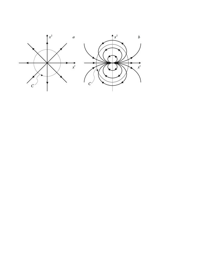
Figure 2: Distribution of unit vector field in the $x:=x^{1},y:=x^{2}$ plane for straight linear disclinations parallel to the $x^{3}$ axis, for $|\Theta|=2\pi$ (a) and $|\Theta|=4\pi$ (b).

A linear disclination is characterized by the Frank vector

$$\Theta_{i}:=\frac{1}{2}\varepsilon_{ijk}\Theta^{jk},$$ (10)

where

$$\Theta^{ij}:=\oint_{C}dx^{\mu}\partial_{\mu}\theta^{ij},$$ (11)

and the integral is taken along closed contour $C$ surrounding the disclination axis. The length of the Frank vector is equal to the total angle of rotation of the field $n^{i}$ as it goes around the disclination. For linear disclinations it must be a multiple of $2\pi$. In the presence of disclinations, the rotational angle field $\theta^{ij}(x)$ is no longer continuous, and we must make some cuts for a given distribution of disclinations and impose appropriate boundary conditions in order to define $\theta^{ij}(x)$. In geometric theory of defects, instead of the rotational angle field, we introduce the ${\mathbb{S}}{\mathbb{O}}(3)$-connection

$$\omega_{\mu}{}^{ij}:=\begin{cases}\partial_{\mu}\omega^{ij},&\text{outside the cut,}\\ {\sf\,lim\,}\partial_{\mu}\omega^{ij},&\text{on the cut.}\end{cases}$$ (12)

in the way similar to the introduction of the triad field. Sure, we assume that the limits on both sides of the cut exist and are equal. So the ${\mathbb{S}}{\mathbb{O}}(3)$-connection is less singular then the rotational angle field by definition.

Then the Frank vector for a surface $S$ is given by the integral of curvature

$$\Omega^{ij}:=\iint_{S}dx^{\mu}\wedge dx^{\nu}R_{\mu\nu}{}^{ij}.$$ (13)

If we have straight linear disclination with rotational symmetry, and vector $n$ rotates in the perpendicular plane, then the ${\mathbb{S}}{\mathbb{O}}(3)$ group reduces to abelian ${\mathbb{S}}{\mathbb{O}}(2)$ group, the nonlinear terms in the curvature (7) disappear, and we return to the previous expression (11) due to the Stokes theorem.

The previous discussion refers to an isolated disclinations. If there is a continuous distribution of disclinations the curvature differs from zero everywhere, and the rotational angle field $\theta^{ij}$ does not exist. Disclinations are said to be absent if and only if the curvature of ${\mathbb{S}}{\mathbb{O}}(3)$-connection vanishes, $R_{\mu\nu i}{}^{j}=0$. In this manner, the geometric theory of defects describes single defects as well as their continuous distribution, in which the phenomena of disclinations is replaced by the notion of curvature.

3 ’t Hooft–Polyakov monopole

Let us consider three-dimensional Euclidean space ${\mathbb{R}}^{3}$ with Cartesian coordinates $x^{\mu}$ and Euclidean metric $\delta_{\mu\nu}$, $\mu,\nu=1,2,3$,. The spherically symmetric ${\mathbb{S}}{\mathbb{U}}(2)$-gauge fields $A_{\mu}{}^{i}$, $i=1,2,3$, interacting with the triplet of scalar fields $\varphi^{i}$ in the adjoint representation minimize the three-dimensional energy [18, 19]

$${\cal E}:=\int\!d^{3}x\left(\frac{1}{4}F^{\mu\nu i}F_{\mu\nu i}+\frac{1}{2}\nabla^{\mu}\varphi^{i}\nabla_{\mu}\varphi_{i}+\frac{1}{4}\lambda\big{(}\varphi^{2}-a^{2}\big{)}^{2}\right),$$ (14)

where indices are raised and lowered by Euclidean metrics $\delta_{\mu\nu}$ and $\delta_{ij}$,

$$\begin{split}F_{\mu\nu}{}^{i}:=&\partial_{\mu}A_{\nu}{}^{i}-\partial_{\nu}A_{\mu}{}^{i}+A_{\mu}{}^{j}A_{\nu}{}^{k}\varepsilon_{jk}{}^{i},\\ \nabla_{\mu}\varphi^{i}:=&\partial_{\mu}\varphi^{i}+A_{\mu}{}^{j}\varphi^{k}\varepsilon_{jk}{}^{i}.\end{split}$$ (15)

– are the curvature tensor components for ${\mathbb{S}}{\mathbb{U}}(2)$-connection and the covariant derivative of scalar fields; $\lambda>0,a>0$ – are coupling constants, $\varepsilon_{ijk}$ is the totally antisymmetric tensor, $\varepsilon_{123}:=1$, and $\varphi^{2}:=\varphi^{i}\varphi_{i}$.

The spherically symmetric ansatz is

$$A_{\mu}{}^{i}=\frac{\varepsilon_{\mu}{}^{ij}x_{j}(K-1)}{r^{2}},\qquad\varphi^{i}=\frac{x^{i}H}{r^{2}},$$ (16)

where $K(r)$ and $H(r)$ are some dimensionless functions on radius $r:=\sqrt{x^{2}}$.

The Euler–Lagrange equations for functional (14) in the spherically symmetric case reduce to

$$\begin{split}r^{2}K^{\prime\prime}=&K\big{(}K^{2}+H^{2}-1\big{)},\\ r^{2}H^{\prime\prime}=&2HK^{2}+\lambda\left(H^{2}-a^{2}r^{2}\right)H.\end{split}$$ (17)

At present we know only one exact analytic solution to this system of equations for $\lambda=0$

$$K=\frac{ar}{{\sf\,sh\,}(ar)},\qquad H=\frac{ar}{\tanh(ar)}-1,$$ (18)

which is called the Bogomol’nyi–Prasad–Sommerfield solution [20, 21]. It is easily checked that this solution has finite energy.

The Lie algebra $\mathfrak{s}\mathfrak{u}(2)$ is isomorphic to $\mathfrak{s}\mathfrak{o}(3)$, and we can consider energy (14) as the three-dimensional Euclidean functional for ${\mathbb{S}}{\mathbb{O}}(3)$-connection interacting with the triplet of scalar fields $\varphi^{i}$ in the fundamental representation. We assume, that this is the expression for the free energy describing static distribution of disclinations and dislocations in elastic media with defects, the triplet of scalar fields being the source of defects.

The Euclidean metric means that elastic stresses are absent in media. The Cartan variables for monopole solutions are

$$e_{\mu}{}^{i}=\delta_{\mu}^{i},\qquad\omega_{\mu}{}^{ij}=A_{\mu}{}^{k}\varepsilon_{k}{}^{ij}=(\delta_{\mu}^{j}x^{i}-\delta_{\mu}^{i}x^{j})\frac{K-1}{r^{2}},$$ (19)

where we use the spherically symmetric ${\mathbb{S}}{\mathbb{O}}(3)$-connection (16). The curvature and torsion are expressed through Cartan variables as usual by Eqs.(6), (7). In the considered case, simple calculations yield the following expressions for curvature and torsion:

$$R_{\mu\nu}{}^{k}:=\frac{1}{2}R_{\mu\nu}{}^{ij}\varepsilon_{ij}{}^{k}=F_{\mu\nu}{}^{k}= \varepsilon_{\mu\nu}{}^{k}\frac{K^{\prime}}{r}-\frac{\varepsilon_{\mu\nu}{}^{j}x_{j}x^{k}}{r^{3}}\left(K^{\prime}-\frac{K^{2}-1}{r}\right),$$ (20)

$$T_{\mu\nu}{}^{k}= \left(\delta_{\mu}^{k}x_{\nu}-\delta_{\nu}^{k}x_{\mu}\right)\frac{K-1}{r^{2}}.$$ (21)

In the geometric theory of defects, curvature (20) and torsion (21) have physical meaning of surface densities of Frank and Burgers vectors, respectively. That is they are equal to $k$-th components of respective vectors on surface element $dx^{\mu}\wedge dx^{\nu}$. If $s^{\mu}$ is normal to the surface element, then there are the following densities of Frank and Burgers vectors:

$$f_{\mu}{}^{i}:= \frac{1}{2}\varepsilon_{\mu}{}^{\nu\rho}R_{\nu\rho}{}^{i}=\frac{1}{3r}\delta_{\mu}^{i}\left(2K^{\prime}+\frac{K^{2}-1}{r}\right)-\frac{1}{r}\left(\hat{x}_{\mu}\hat{x}^{i}-\frac{1}{3}\delta_{\mu}^{i}\right)\left(K^{\prime}-\frac{K^{2}-1}{r}\right),$$ (22)

$$b_{\mu}{}^{i}:= \frac{1}{2}\varepsilon_{\mu}{}^{\nu\rho}T_{\nu\rho}{}^{i}=\varepsilon_{\mu}{}^{ij}\hat{x}_{j}\frac{K-1}{r},$$ (23)

where $\hat{x}^{\mu}:=x^{\mu}/r$ and tensor $f_{\mu}{}^{i}$ is decomposed into irreducible components.

For the Bogomol’nyi–Prasad–Sommerfield solution functions $K(r)$ and $H(r)$ are given in Eq. (18). They have the following asymptotics

$$K\big{|}_{r\to 0}\approx 1-\frac{(ar)^{2}}{6}-\frac{(ar)^{4}}{120}, \qquad K\big{|}_{r\to\infty}\approx 2ar{\sf\,e}^{-ar}\to 0,$$ (24)

$$H\big{|}_{r\to 0}\approx 1+\frac{(ar)^{2}}{3}-\frac{2(ar)^{4}}{15}, H\big{|}_{r\to\infty}\approx ar-1\to\infty.$$

The corresponding asymptotics of Frank and Burgers vector densities are

$$\begin{split}f_{\mu}{}^{i}\big{|}_{r\to 0}\approx&-\frac{1}{3}\delta_{\mu}^{i}\left(a^{2}+\frac{7}{90}a^{4}r^{2}\right)+\frac{2}{45}x_{\mu}x^{i}3a^{4}\to-\frac{1}{3}\delta_{\mu}^{i}a^{2},\\ b_{\mu}{}^{i}\big{|}_{r\to 0}\approx&-\frac{1}{6}\varepsilon_{\mu}{}^{ij}x_{j}\left(a^{2}+\frac{a^{4}r^{2}}{20}\right)\to-\frac{1}{6}\varepsilon_{\mu}{}^{ij}x_{j}a^{2},\\ \varphi^{i}\big{|}_{r\to 0}\approx&\frac{1}{3}x^{i}\left(a^{2}-\frac{2a^{4}r^{2}}{5}\right)\to\frac{1}{3}x^{i}a^{2},\\ f_{\mu}{}^{i}\big{|}_{r\to\infty}\approx&-\frac{x_{\mu}x^{i}}{r^{4}}\to 0,\\ b_{\mu}{}^{i}\big{|}_{r\to\infty}\approx&-\varepsilon_{\mu}{}^{ij}x_{j}\frac{1}{r^{2}}\to 0,\\ \varphi^{i}\big{|}_{r\to\infty}\approx&\frac{x^{i}}{r}\left(a-\frac{1}{r}\right)\to\frac{x^{i}}{r}a.\end{split}$$ (25)

It implies, in particular, that the total energy (14) is finite.

4 Conclusion

The geometric theory of defects is aimed for description of dislocations and disclinations in the continuous approximation. It is well suited for description of single defects as well as their continuous approximation. In the present paper, we consider media with Euclidean metric but nontrivial ${\mathbb{S}}{\mathbb{O}}(3)$-connection. The ’t Hooft–Polyakov monopole solution is the static spherically symmetric solution of ${\mathbb{S}}{\mathbb{U}}(2)$ Yang–Mills theory. The isomorphism of $\mathfrak{s}\mathfrak{u}(2)$ and $\mathfrak{s}\mathfrak{o}(3)$ Lie algebras implies that the ’t Hooft–Polyakov monopole may have new physical interpretation in solid state physics. In contrast to the original model, the ${\mathbb{S}}{\mathbb{O}}(3)$ group acts now not in the isotopic space but in the tangent space, giving rise to nontrivial torsion and curvature. These geometrical notions have physical interpretation as surface densities of Burgers and Frank vectors, respectively, in the geometric theory of defects. These are explicitly computed for the Bogomol’nyi–Prasad–Sommerfield solution. We are not aware what kind of media is to be chosen for experimental observations and what kind of experiment can be taken to confirm or disprove the geometric theory of defects but the mere existence of such possibility seems to be interesting.

References

- [1] L. D. Landau and E. M. Lifshits. Theory of Elasticity. Pergamon, Oxford, 1970.
- [2] A. M. Kosevich. Physical mechanics of real crystals. Naukova dumka, Kiev, 1981. [in Russian].
- [3] J. M. Burgers. Proc. Kon. Ned. Akad. Wetenschap., 42:293–378, 1939.
- [4] J. M. Burgers. Proc. Kon. Ned. Akad. Wetenschap., 42:378–398, 1939.
- [5] F. C. Frank. On the theory of liquid crystals. Discussions Farad. Soc., 25:19–28, 1958.
- [6] M. O. Katanaev and I. V. Volovich. Theory of defects in solids and three-dimensional gravity. Ann. Phys., 216(1):1–28, 1992.
- [7] M. O. Katanaev. Geometric theory of defects. Physics – Uspekhi, 48(7):675–701, 2005. https://arxiv.org/abs/cond-mat/0407469.
- [8] K. Kondo. On the geometrical and physical foundations of the theory of yielding. In Proc. 2nd Japan Nat. Congr. Applied Mechanics, pages 41–47, Tokyo, 1952.
- [9] J. F. Nye. Some geometrical relations in dislocated media. Acta Metallurgica, 1:153, 1953.
- [10] B. A. Bilby, R. Bullough, and E. Smith. Continuous distributions of dislocations: a new application of the methods of non-Riemannian geometry. Proc. Roy. Soc. London, A231:263–273, 1955.
- [11] E. Kröner. Kontinums Theories der Versetzungen und Eigenspanungen. Spriger–Verlag, Berlin – Heidelberg, 1958.
- [12] H. Kleinert. Multivalued Fields in Condenced Matter, Electromagnetism, and Gravitation. World Scientific, Singapore, 2008.
- [13] M. O. Katanaev and I. V. Volovich. Scattering on dislocations and cosmic strings in the geometric theory of defects. Ann. Phys., 271:203–232, 1999.
- [14] M. O. Katanaev. Wedge dislocation in the geometric theory of defects. Theor. Math. Phys., 135(2):733–744, 2003.
- [15] M. O. Katanaev. One-dimensional topologically nontrivial solutions in the Skyrme model. Theor. Math. Phys., 138(2):163–176, 2004.
- [16] G. ’t Hooft. Magnetic monopoles in unified gauge theories. Nucl. Phys. B, 79(2):276–284, 1974.
- [17] A. M. Polyakov. Particle spectrum in the quantum field theory. JETP Letters, 20(6):194–195, 1974.
- [18] N. Manton and P. Sutcliffe. Topological Solitons. Cambridge University Press, Cambridge, 2004.
- [19] Ya. Shnir. Magnetic Monopoles. Springer–Verlag, Berlin, Heidelberg, 2005.
- [20] M. K. Prasad and C. H. Sommerfield. Exact classical solution for the ’t hooft monopole and the julia-zee dyon. Phys. Rev. Lett., 35:760–762, 1975.
- [21] E. B. Bogomol’nyi. The stability of classical solutions. Sov. J. Nucl. Phys., 24(4):449, 1976.
- [22] M. O. Katanaev. Chern–Simons term in the geometric theory of defects. Phys. Rev. D, 96:84054, 2017. https://doi.org/10.1103/PhysRevD.96.084054 https://arxiv.org/abs/1705.07888 [gr-qc].