On the Energy Sources of the Most Luminous Supernova ASASSN-15lh

Abstract

In this paper, we investigate the energy-source models for the most luminous supernova ASASSN-15lh. We revisit the ejecta-circumstellar medium (CSM) interaction (CSI) model and the CSI plus magnetar spin-down with full gamma-ray/X-ray trapping which were adopted by Chatzopoulos et al. (2016) and find that the two models cannot fit the bolometric LC of ASASSN-15lh. Therefore, we consider a CSI plus magnetar model with the gamma-rays/X-rays leakage effect to eliminate the late-time excess of the theoretical LC. We find that this revised model can reproduce the bolometric LC of ASASSN-15lh. Moreover, we construct a new hybrid model (i.e., the CSI plus fallback model), and find that it can also reproduce the bolometric LC of ASASSN-15lh. Assuming that the conversion efficiency ($\eta$) of fallback accretion to the outflow is typically $\sim 10^{-3}$, we derive that the total mass accreted is $\sim 3.9~{}M_{\odot}$. The inferred CSM mass in the two models is rather large, indicating that the progenitor could have experienced an eruption of hydrogen-poor materials followed by an energetic core-collapse explosion leaving behind a magnetar or a black hole.

1 Introduction

In the past two decades, more than 100 super-luminous supernovae (SLSNe) have been found (Gal-Yam, 2012, 2019; Inserra, 2019) by several sky-survey projects for optical transients (see, e.g., Chomiuk et al. 2011; Quimby et al. 2011; Nicholl et al. 2014; Quimby 2014; De Cia et al. 2018; Lunnan et al. 2018; Angus et al. 2019). Just like normal supernovae (SNe), SLSNe can be classified as types I and II, depending on whether the spectra contains hydrogen absorption lines or not. In addition to their luminosity, the main difference between SLSNe and normal SNe is their energy sources. Most normal SNe can be explained by the ⁵⁶Ni cascade decay model that doesn’t apply to almost all SLSNe. The energy sources of SLSNe are still elusive. The pair instability SN (PISN) model (Barkat et al., 1967; Rakavy & Shaviv, 1967; Heger & Woosley, 2002; Heger et al., 2003) was suggested to account for some SLSNe, while the magnetar spin-down model (Kasen & Bildsten, 2010; Inserra et al., 2013; Nicholl et al., 2013, 2014; Wang et al., 2015, 2016), the ejecta-circumstellar medium (CSM) interaction (CSI) model (Chevalier, 1982; Chevalier & Fransson, 1994; Chevalier & Irwin, 2011; Chatzopoulos et al., 2012; Liu et al., 2018), and the fallback model (Dexter & Kasen, 2013) were used to explain most of SLSNe (see Moriya et al. 2018; Wang et al. 2019b and references therein).

To date, the most luminous SLSN might be ASASSN-15lh, which was an extremely luminous optical-UV transient discovered by All-Sky Automated Survey for SuperNovae (ASAS-SN, Shappee et al. 2014) on June 14, 2015 (Dong et al., 2016). At early times ($t<30$ days, rest frame adopted throughout), there are only $V$ band data observed by ASAS-SN. The multi-band follow-up observations were performed by the $V$ and $B$ filters of the Las Cumbres Observatory Global Telescope Network (LCOGT; Brown et al. 2013) and $V$, $B$, $U$, $UVW1$, $UVM2$, and $UVW2$ filters of the UltraViolet and Optical Telescope (UVOT) on board the Neil Gehrels Swift Observatory (Swift, Gehrels et al. 2004; Roming et al. 2005). The UV observations performed by UVOT last from 30 to 450 days except for the sun constraint break ($230-240$ days). The UVOT $V$- and $B$-band observations were sometimes interrupted, but the LCOGT $V$- and $B$-band observations were always used when needed.

Based on the blackbody assumption, Dong et al. (2016) and Godoy-Rivera et al. (2017) used the multi-band LCs to fit the early-time and the whole bolometric LCs, respectively. For the very early epoch ($t<30$ days), Godoy-Rivera et al. (2017) adopted two different evolution modes of the blackbody temperature, i.e., a linearly increasing temperature in a logarithmic scale and a constant temperature, to obtain the corresponding bolometric LCs. At a redshift of $z=0.2326$, ASASSN-15lh reached a peak bolometric luminosity of $(2.2\pm 0.2)\times 10^{45}\rm\ erg\ s^{-1}$, more than twice as luminous as any previously known SNe. After the main peak lasted for $\sim 90$ days, there was a rebrightening of Swift UV bands, and the bolometric LC showed a $\sim 120$ days plateau, and then faded again (Godoy-Rivera et al., 2017). The total radiation energy of ASASSN-15lh is $\sim 1.7-1.9\times 10^{52}$ erg over the $\sim 450$ days since the first detection (Godoy-Rivera et al., 2017). Besides, at the location of ASASSN-15lh, a persistent X-ray emission whose luminosity is $\sim 10^{41}-10^{42}\rm\ erg\ s^{-1}$ was observed by the Chandra X-ray observatory (Margutti et al., 2017).

The nature of ASASSN-15lh is still in debate. Dong et al. (2016) classified ASASSN-15lh as a hydrogen-poor (type I) SLSN; after analyzing the entire evolution of photospheric radius as well as the radiated energy and estimating the event rate, Godoy-Rivera et al. (2017) thought ASASSN-15lh is more similar to a H-poor SLSN rather than a TDE. On the other hand, Leloudas et al. (2016) and Krühler et al. (2018) claimed that it is a tidal disruption event (TDE).

The extremely high peak luminosity, long duration, and exotic bolometric LC challenge all existing energy-source models for SLSNe. Dong et al. (2016) estimated that at least $30~{}M_{\odot}$ of ⁵⁶Ni is required to produce the observed peak luminosity of ASASSN-15lh if the LC was powered by ⁵⁶Ni cascade decay, while Kozyreva et al. (2016) showed that $1500~{}M_{\odot}$ of ⁵⁶Ni is needed to power the bolometric LC based on numerical simulation. Some other authors (Metzger et al., 2015; Dai et al., 2016; Bersten et al., 2016; Sukhbold & Woosley, 2016) suggested that a magnetar with extremely rapid rotation can drive the early-time extremely luminous bolometric LC of ASASSN-15lh. Chatzopoulos et al. (2016) showed that a CSI model with ejecta mass of $\sim 35~{}M_{\odot}$ and CSM mass of $\sim 20~{}M_{\odot}$ could reproduce the first $\sim 220$ days of the bolometric LC, i.e., the main peak and the plateau. However, the entire bolometric LC of ASASSN-15lh spanning $\sim 450$ days has not been modeled by the models mentioned above. Recently, Mummery & Balbus (2020) fitted the multi-band light curves of ASASSN-15lh using the TDE model involving a super-massive maximally rotating black hole whose mass is $\sim 10^{9}$ M_⊙.

In this paper, we investigate several possible energy sources of ASASSN-15lh. In section 2, three models are used to reproduce the bolometric LC of ASASSN-15lh. Our discussion and conclusions can be found in Sections 3 and 4, respectively.

2 Modeling the Bolometric LC of ASASSN-15lh

In this section, we use three energy-source models (the CSI model, the CSI plus magnetar model, and the CSI plus fallback model) to fit the bolometric LC of ASASSN-15lh which is taken from Godoy-Rivera et al. (2017). It should be noted that the bolometric LC at $t<30$ days is constructed by assuming a logarithmic linearly increasing temperature Godoy-Rivera et al. (2017). For each model, both the wind-like CSM ($s=2$) and dense-shell CSM ($s=0$) are taken into account. The value of the optical opacity $\kappa$ of the hydrogen-poor ejecta and the CSM is fixed to be $0.2\rm\ cm^{2}\ g^{-1}$ throughout this paper, the conversion efficiency of the kinetic energy to radiation is assumed to be 100% (Chatzopoulos et al., 2013).

We develop our own Python-based semi-analytic models and use them to fit the bolometric LC of ASASSN-15lh. Bayesian analysis is adopted to determine the best fitting parameters. We use the emcee python package (Foreman-Mackey et al., 2013) based on Markov Chain Monte Carlo (MCMC) by performing a maximum likelihood $\chi^{2}$ fit, and provides the posterior probability distributions for the free parameters in these models. The free parameters and priors in our models can be seen in Table 1. We ran the MCMC with 20 walkers for running 100,000 steps. Once the MCMC is done, the best fit values and the uncertainties are computed as the 16th, 50th, and 84th percentiles of the posterior samples along each dimension, i.e., the uncertainties are measured as $1\sigma$ confidence ranges.

2.1 The CSI Model

Chatzopoulos et al. (2016) pointed out that the CSI model can explain the first $\sim 220$ days bolometric LC of ASASSN-15lh. To verify whether the model can explain the $\sim 450$ days bolometric LC, we use the same model the whole LC. The semi-analytical CSI model adopted here was discussed by Chatzopoulos et al. (2012), Chatzopoulos et al. (2013) and Wang et al. (2019a). Since the ASASSN-15lh is a type I SN, $n=7$ and $\delta=0$ are adopted for the ejecta outer and inner density profiles.

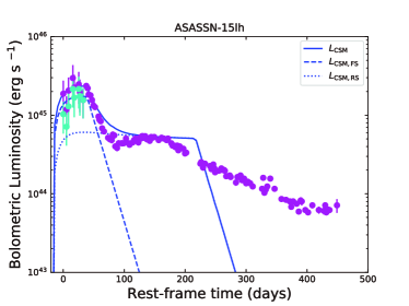
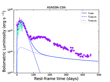
Figure 1: The bolometric LCs of ASASSN-15lh reproduced by the CSI model: $s=0$ (the left panel) and $s=2$ (the right panel). The total luminosity ($L_{\rm tot}$) are shown by solid blue curves and the contributions from the forward shock ($L_{\rm CSI,FS}$) and the reverse shock ($L_{\rm CSI,RS}$) are shown by dashed and dotted blue curves, respectively. Data are taken from Godoy-Rivera et al. (2017), where the first eight data points was derived based on the assumptions of the rising-temperature feature (magenta) and constant temperature feature (cyan), respectively.

Finally, the CSI model has 7 free parameters: $M_{\rm{ej}}$, $v_{\rm{SN}}$, $M_{\rm{CSM}}$, $\rho_{\rm{CSM,in}}$, $R_{\rm CSM,in}$, $x_{0}$, and the moment of explosion $t_{\rm{expl}}$. The theoretical bolometric LCs are shown in Figure 1. It can be found that this model cannot reproduce the entire luminosity evolution: in the case of wind-like CSM, the CSI model can only reproduce the main peak; in the case of dense-shell CSM, the CSI model cannot reproduce the late-time decline of bolometric LC of ASASSN-15lh.

2.2 The CSI Plus Magnetar Model

Chatzopoulos et al. (2016) also adopted the CSI plus magnetar model to model the first $\sim 220$ days LC of ASASSN-15lh. Here we use the same model to model the whole bolometric LC.

For the semi-analytical CSI plus magnetar model, there are two cases for the output luminosity: a homogeneously expanding photosphere and a fixed photosphere. The former is applied to some centrally located energy sources (e.g., the ⁵⁶Ni cascade decay, the magnetar spin-down radiation and the fallback accretion outflow) heating the expansive SN ejecta, while the latter is mainly applied to the CSI model, in which the nearly stationary CSM relative to the ejecta is heated.

We next consider a CSI plus magnetar model to fit the bolometric LC of ASASSN-15lh. We divide the radiative process into two phases: the early-time fixed-photosphere phase before the ejecta sweeps up the CSM and the late-time homogeneously expanding-photosphere phase after the ejecta sweeps up the CSM, respectively. We suppose that the CSI dominates the early peak of the bolometric LC before 90 days, and the late-time plateau and subsequent phase after ejecta sweeps up the optically thick CSM were mainly powered by the magnetar spin-down. The total ejecta mass at the late epoch becomes $M_{\rm ej}+M_{\rm CSM,th}$. Based on these assumptions, the CSI plus magnetar model we adopt can be expressed by

$$L(t)=\frac{1}{t_{0}}e^{-\frac{t}{t_{0}}}\int_{t_{\rm expl}}^{t+t_{\rm expl}}e^{\frac{t^{\prime}}{t_{0}}}\left[L_{\rm inp,FS}(t^{\prime})+L_{\rm inp,RS}(t^{\prime})\right]dt^{\prime}+\frac{2}{t_{d}}e^{\frac{t^{2}}{t_{d}^{2}}}\int_{t_{\rm expl}}^{t+t_{\rm expl}}e^{\frac{t^{\prime 2}}{t_{d}^{2}}}L_{\rm inp,mag}(t^{\prime})dt^{\prime},$$ (1)

where $L_{\rm inp,FS}(t)$ and $L_{\rm inp,RS}(t)$ are the input luminosities from the forward shock and reverse shock, respectively (Chatzopoulos et al., 2012); $L_{\rm inp,mag}(t)$ is the input luminosity from the magnetar spin-down (Kasen & Bildsten, 2010), $t_{0}$ and $t_{d}=[\frac{2\kappa(M_{\rm ej}+M_{\rm CSM,th})}{\beta cv_{\rm SN}}]^{1/2}$ are the effective LC timescales in a fixed photosphere and an expanding photosphere, respectively (Chatzopoulos et al., 2012).

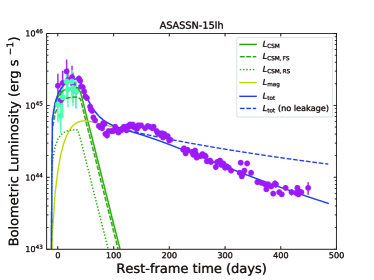
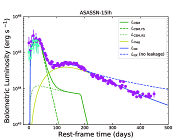
Figure 2: The bolometric LCs of ASASSN-15lh reproduced by the CSI plus magnetar model: $s=0$ (the left panel) and $s=2$ (the right panel). The total luminosity ($L_{\rm tot}$) are shown by solid blue curves and the contributions from the forward shock ($L_{\rm CSI,FS}$), the reverse shock ($L_{\rm CSI,RS}$), and the magnetar spin-down ($L_{\rm mag}$) are shown in dashed green, dotted green, and solid yellow curves, respectively. The dashed blue curves represent the total luminosity that the leakage effect is not taken into account. Data are taken from Godoy-Rivera et al. (2017).

The CSI plus magnetar model has 9 free parameters: $M_{\rm{ej}}$, $v_{\rm{SN}}$, $P_{0}$, $B_{p}$, $M_{\rm{CSM}}$, $\rho_{\rm{CSM,in}}$, $R_{\rm CSM,in}$, $x_{0}$, and $t_{\rm{expl}}$. The LC produced by the CSI plus magnetar model are shown in dashed blue lines in Figure 2. We find that the CSI+magnetar model used by Chatzopoulos et al. (2016) cannot reproduce the entire luminosity evolution since the late-time theoretical LCs produced by both the shell-CSI and the wind-CSI are brighter than the observations.

To eliminate the late-time excess, we employ a CSI plus magnetar model by considering the leakage effect of gamma-ray/X-rays from the magnetar (Wang et al., 2015) which can be described as

$$L(t)=\frac{1}{t_{0}}e^{-\frac{t}{t_{0}}}\int_{t_{\rm expl}}^{t+t_{\rm expl}}e^{\frac{t^{\prime}}{t_{0}}}\left[L_{\rm inp,FS}(t^{\prime})+L_{\rm inp,RS}(t^{\prime})\right]dt^{\prime}+\frac{2}{t_{d}}e^{\frac{t^{2}}{t_{d}^{2}}}\int_{t_{\rm expl}}^{t+t_{\rm expl}}e^{\frac{t^{\prime 2}}{t_{d}^{2}}}L_{\rm inp,mag}(t^{\prime})\left(1-e^{-\tau_{\rm\gamma,mag}}\right)dt^{\prime},$$ (2)

where $e^{-\tau_{\rm\gamma,mag}}$ and $1-e^{-\tau_{\rm\gamma,mag}}$ are the leaking factor and the trapping factor which represent the gamma-ray/X-ray leakage and trap from the magnetar, respectively; $\tau_{\rm\gamma,mag}$ is the optical depth of the ejecta to gamma-ray/X-ray emissions which can be written as $\tau_{\rm\gamma,mag}=\frac{3\kappa_{\rm\gamma,mag}(M_{\rm ej}+M_{\rm CSM})}{4\pi v_{SN}^{2}t^{2}}$, $\kappa_{\rm\gamma,mag}$ is the opacity of the gamma-ray/X-ray generated by magnetar spinning-down.

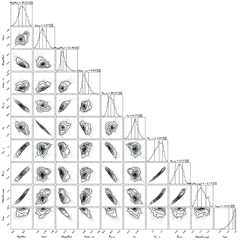
Figure 3: The corner plot for the CSI plus magnetar model ($s=2$).

The CSI plus magnetar model taking into account the gamma/X-ray leakage effect has 10 free parameters: $M_{\rm{ej}}$, $v_{\rm{SN}}$, $P_{0}$, $B_{p}$, $\kappa_{\gamma,\rm{mag}}$, $M_{\rm{CSM}}$, $\rho_{\rm{CSM,in}}$, $R_{\rm CSM,in}$, $x_{0}$, and $t_{\rm{expl}}$. The LCs produced by the CSI plus magnetar model are shown in solid blue curves in Figure 2 and the best-fitting parameters are listed in Table 2. Figure 3 is the corner plots showing the results of our MCMC parameter estimation for the CSI plus magnetar model ($s=2$). The shape of the two dimensional projections of the posterior probability distributions indicates the correlations between the parameters: the closer to a circle, the more independent the parameters are; the closer to a slender shape, the more correlated the parameters are. We note that there are many pairs of parameters show degeneracies, which means there are many combinations of these degenerate parameters to achieve the same fitting result. This usually makes the best fitting parameters more uncertain. Therefore, although the semi-analytic model successfully reproduce the luminosity evolution, one should treat these best fitting parameters with caution.

The results show that the dense-shell case cannot reproduce the plateau phase and the value of reduced $\chi^{2}$ ($\chi^{2}/\rm dof\sim 5$) is higher than that of the wind-like CSM model ($\chi^{2}/\rm dof\sim 2$) which can reproduce the main peak, plateau, and late-time decline. The best-fitting parameters are $M_{\rm ej}\sim 40~{}M_{\odot}$, $M_{\rm CSM}\sim 21~{}M_{\odot}$, and $v_{\rm SN}\sim 16,000\rm\ km\ s^{-1}$. Using $E_{\rm SN}=\frac{(3-\delta)(n-3)}{2(5-\delta)(n-5)}M_{\rm ej}(x_{0}v_{\rm SN})^{2}$, we derived the kinetic energy of the SN ejecta $E_{\rm SN}\sim 7.0\times 10^{52}\rm\ erg$. Besides, a magnetar with initial spin period $P_{0}\sim 1.1\rm\ ms$ and the magnetic field strength $B_{p}\sim 1.7\times 10^{13}\rm\ G$ is needed to reproduce the late-time plateau and decline.

2.3 The CSI Plus Fallback Model

Here we propose an alternative model, in which the bolometric LC of ASASSN-15lh is supposed to be due to the jointing effect of the CSI and fallback accretion. In this scenario, the main peak, the subsequent plateau, and the renewed decline at $\gtrsim 200$ days since its detection are powered by CSI forward shock, the CSI reverse shock, and the late-time black-hole fallback accretion, respectively. The LC of this energy source model has the following form,

$$L(t)=\frac{1}{t_{0}}e^{-\frac{t}{t_{0}}}\int_{t_{\rm expl}}^{t+t_{\rm expl}}e^{\frac{t^{\prime}}{t_{0}}}\epsilon[L_{\rm inp,FS}(t^{\prime})+L_{\rm inp,RS}(t^{\prime})]dt^{\prime}+\frac{2}{t_{d}}e^{\frac{t^{2}}{t_{d}^{2}}}\int_{t_{\rm fb}-t_{\rm expl}}^{t+t_{\rm fb}-t_{\rm expl}}e^{\frac{t^{2}}{t_{d}^{2}}}L_{\rm inp,fb}(t^{\prime})dt^{\prime}.$$ (3)

where $t_{0}$ and $t_{d}$ are described in subsection 2, $t_{\rm{fb}}$ is the time when fallback accretion begins. Generally, fallback accretion may happen at the beginning of explosion, when the materials with expansion velocity less than the escape velocity are eventually accreted onto the central compact remnant. The accretion rate is usually flat at early times ($\lesssim 10^{3}$ s), which is related to free-fall accretion, proportional to $t^{-5/3}$ at late times (Michel, 1988; Chevalier, 1989; Zhang et al., 2008; Dexter & Kasen, 2013). Numerical fallback simulations (Chevalier, 1989; Zhang et al., 2008; Dexter & Kasen, 2013) showed that the reverse shock forms when the ejecta meets the outer shell. The reverse shock can decelerate the ejecta and enhance the fallback rate, but the late-time accretion rate is still proportional to $t^{-5/3}$. Here, we consider a late-time enhanced fallback accretion due to the CSI reverse shock and suppose that the enhanced fallback accretion occurs at $t_{\rm{fb}}$ after the SN explosion.

The accretion usually accompanied by an outflow carrying huge amount of energy. The power input by the outflow associated with fallback accretion can be expressed by

$$L_{\rm{inp,fb}}(t)=L_{\rm{fb,0}}\left(\frac{t}{t_{\rm{fb}}-t_{\rm expl}}\right)^{-5/3},$$ (4)

where $L_{\rm{fb,0}}$ is the initial input power driven by fallback. Here, we assume the energy input from fallback is 100% thermalized.

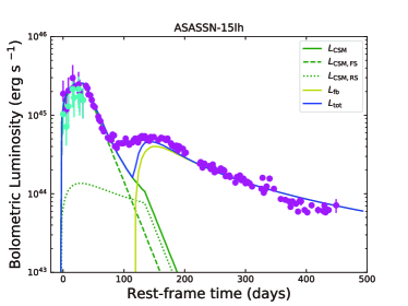
Figure 4: The bolometric LCs of ASASSN-15lh reproduced by the CSI plus fallback model: $s=0$ (the left panel) and $s=2$ (the right panel). The total luminosity ($L_{\rm tot}$) are shown by solid blue curves. The contributions from the forward shock ($L_{\rm CSI,FS}$), the reverse shock ($L_{\rm CSI,RS}$), and the fallback accretion ($L_{\rm fb}$) are shown by dashed green, dotted green, and solid yellow curves, respectively. Data are taken from Godoy-Rivera et al. (2017).

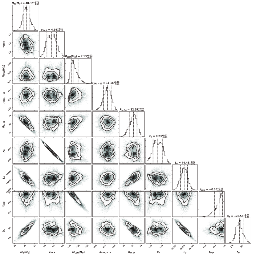
Figure 5: The corner plot for the CSI plus fallback model ($s=0$).

The CSI plus fallback model includes the following 9 parameters: $M_{\rm{ej}}$, $v_{\rm{SN}}$, $M_{\rm{CSM}}$, $\rho_{\rm{CSM,in}}$, $R_{\rm CSM,in}$, $x_{0}$, $L_{\rm{fb,0}}$, $t_{\rm{fb}}$, and $t_{\rm expl}$. The LCs produced by the model are shown in Figure 4 and the best-fitting parameters are listed in Table 3. Figure 5 is the corner plots showing the results of our Markov Chain Monte Carlo parameter estimation for the CSI plus fallback model ($s=0$).

The bolometric LC of ASASSN-15lh can only be fitted in the shell case with $\chi^{2}/\rm dof\sim 4$. The wind case fails to reproduce the plateau and the value of $\chi^{2}/\rm dof$ is $\sim 9$. The derived values of $M_{\rm ej}$, $M_{\rm CSM}$, $v_{\rm SN}$, and $E_{\rm SN}$ are $\sim 40~{}M_{\odot}$, $\sim 7~{}M_{\odot}$, $\sim 41,000\rm\ km\ s^{-1}$, and $\sim 4.5\times 10^{52}\rm\ erg$, respectively.

Using $L_{\rm{fb,0}}$ and $t_{\rm{fb}}$, we can derive the total input energy

$$E_{\rm{fb}}=\int_{t_{\rm{fb}}-t_{\rm{expl}}}^{+\infty}L_{\rm{fb,0}}\left(\frac{t}{t_{\rm{fb}}-t_{\rm{expl}}}\right)^{-5/3}\ dt=1.5L_{\rm{fb,0}}(t_{\rm{fb}}-t_{\rm{expl}}).$$ (5)

The value $E_{\rm{fb}}$ is $\sim 7.0\times 10^{51}$ erg. Dexter & Kasen (2013) estimated that the typical value of the conversion efficiency of the fallback accretion energy to outflow energy $\eta$ is $\sim 10^{-3}$. Adopting this value, we find that the total mass of accretion $M_{\rm{fb}}=E_{\rm{fb}}/\eta c^{2}$ is $\sim 3.9~{}M_{\odot}$, indicating that only about a tenth of the ejecta finally fell back. The accretion rate range from $5.3~{}M_{\odot}\ \rm{yr}^{-1}$ to $1.1~{}M_{\odot}\ \rm{yr}^{-1}$ after 180 to 450 days since the explosion.

3 Discussion

3.1 Progenitor and Explosion Scenarios

In Section 2, we have demonstrated that both the ejecta-wind interaction plus magnetar spin-down with hard emission leakage model and the ejecta-shell interaction plus black hole fallback accretion model can reproduce the bolometric LC of ASASSN-15lh. The required total (SN ejecta + CSM) mass are $\sim 61~{}M_{\odot}$ and $\sim 47~{}M_{\odot}$ in the two models, respectively. The results are consistent with those of Chatzopoulos et al. (2016), suggesting that the explosion scenario would be a rapidly rotating pulsational pair-instability supernova (PPISN; Chatzopoulos et al. 2012) or a progenitor related with a luminous blue variable (LBV; Smith & Owocki 2006). For the CSI plus magnetar model, what one should caution is that the formation a magnetar rather than a black hole is difficult for a progenitor with mass large than $\sim 61~{}M_{\odot}$ (Heger & Woosley, 2002). It is believed that very massive stars would produce stellar-mass black holes. However, some magnetars might come from very massive progenitors (e.g., Muno et al. 2006 showed that an X-ray pulsar in the young massive cluster Westerlund 1 has a very massive progenitor $>40~{}M_{\odot}$), indicating that the CSI plus magnetar model cannot be ruled out by the large derived total mass.

After pulsational eruptions of hydrogen-poor materials, the progenitor might experiences energetic core-collapse explosion. The values of the kinetic energy inferred by the CSI plus magnetar model and the CSI plus fallback model are $\sim 7.0\times 10^{52}\rm\ erg$ and $\sim 4.5\times 10^{52}\rm\ erg$, respectively. These values are greater than the explosion energy $\sim 10^{51}$ erg gotten by the neutrino-driven process. However, some so-called “hypernovae” having kinetic energy comparable to the values inferred above have been discovered.

The large kinetic energy derived by the CSI plus magnetar model deserves further discussion. In the magnetar model, magnetar spinning-down process would convert a fraction of the rotational energy to the kinetic energy of the ejecta (see, e.g., Wang et al. 2016). However, the fraction of the rotational energy converted to the kinetic energy depends on the spin-down timescale: a magnetar having a short spin-down timescale converts most of its rotational energy to the kinetic energy of the ejecta, while a magnetar with long spin-down timescale converts a minor fraction of its rotational energy to the kinetic energy of the ejecta and most of the rotational energy would be converted to radiation. The spin-down timescale of the magnetar in our model is $\sim 216$ days, which is much larger than the diffusion timescale $t_{d}$ which is $\sim 100$ days. Therefore, the magnetar in our model would convert most of its rotational energy to radiation rather than the kinetic energy of the ejecta, i.e., the kinetic energy of the ejecta didn’t come from the magnetar.

3.2 The Mass Loss History of the Progenitor of ASASSN-15lh

It is interesting to infer the mass-loss history of the progenitor of ASASSN-15lh. For the ejecta-wind interaction plus magnetar model, assuming that the velocity of the wind ($v_{\rm w}$) is $100-1000\rm\ km\ s^{-1}$, we find that the mass loss rate $\dot{M}=4\pi v_{\rm w}q$ ($q=\rho_{\rm CSM,in}R_{\rm CSM,in}^{2}$) of the stellar wind is $\dot{M}\sim 0.9-9~{}M_{\odot}\ \rm{yr}^{-1}$. This mass loss rate is larger than the typical value $\sim 0.1-2~{}M_{\odot}\ \rm{yr}^{-1}$ of the other SN progenitors (Chugai & Danziger, 2003; Chugai et al., 2004; Ofek et al., 2014; Nyholm et al., 2017). But it can be explained in the light of “superwinds” (Moriya et al., 2020).

We can also estimate the time interval between the last eruption and the SN explosion is $\Delta t\sim 2-25$ years by using $\Delta t=R_{\rm CSM,in}/v_{\rm w}$, which is similar to those of SLSN PS1-12cil and SN 2012aa (Li et al., 2020). Before this time, the progenitor has spent $M_{\rm CSM}/\dot{M}\sim 2.4-24$ years for stellar-wind mass loss. For the ejecta-shell interaction plus fallback model, assuming that the velocity of the wind ($v_{\rm shell}$) is $100-1000\rm\ km\ s^{-1}$, we see that the time interval between the eruption of shell and the SN explosion is $R_{\rm CSM,in}/v_{\rm shell}\sim 1-10$ years.

4 Conclusions

ASASSN-15lh might be the most luminous SN discovered to date. Its extremely high peak luminosity, long duration, and the exotic shape of bolometric LC challenge the existing energy-source models for SLSNe. There are many studies for the energy source of ASASSN-15lh, but the entire luminosity evolution of ASASSN-15lh has not been studied by the models assuming that ASASSN-15lh is an SLSN.

In this paper, we fitted the whole bolometric LC of ASASSN-15lh by using several models taking into account the CSI contribution. According to the physical properties of the CSM, the models are considered in two cases: the dense-shell CSM ($s=0$) and wind-like CSM ($s=2$). The MCMC method was adopted to obtain the best fitting result.

We find that both the CSI model and the CSI plus magnetar model with full full gamma-ray/X-rays trapping which were used by Chatzopoulos et al. (2016) cannot reproduce the whole LC. To eliminate the late-time excess, we proposed a CSI plus magnetar model with considering the leakage effect of gamma-ray/X-rays from the magnetar and found that the model can well reproduce the overall bolometric LC of ASASSN-15lh if the CSM is a wind ($s=2$). The parameters we derived are $M_{\rm ej}\sim 40~{}M_{\odot}$, $M_{\rm CSM}\sim 21~{}M_{\odot}$, $v_{\rm SN}\sim 16,000\rm\ km\ s^{-1}$, $P_{0}\sim 1.1\rm\ ms$, $B_{p}\sim 1.7\times 10^{13}\rm\ G$, $E_{\rm SN}\sim 7.0\times 10^{52}\rm\ erg$. The stellar wind with mass-loss rate $\dot{M}\sim 0.9-9~{}M_{\odot}\ \rm{yr}^{-1}$ could have been expelled from progenitor in $\sim 2.4-24$ years, and ceased at $\sim 2-25$ years before explosion.

We also proposed a new hybrid model, the CSI plus fallback model, and applied it to the LC of ASASSN-15lh. In this scenario, the luminosity evolution of ASASSN-15lh can only be explained in the shell case ($s=0$). The parameters we derived are $M_{\rm ej}\sim 40~{}M_{\odot}$, $M_{\rm CSM}\sim 7~{}M_{\odot}$, $v_{\rm SN}\sim 41,000\rm\ km\ s^{-1}$, and $E_{\rm SN}\sim 4.5\times 10^{52}\rm\ erg$. Assuming that the the conversion efficiency ($\eta$) of the fallback accretion to the outflow is $\sim 10^{-3}$ which is a typical value, we find that the total mass of accretion is $\sim 3.9~{}M_{\odot}$. Furthermore, the time interval between the eruption of shell and the SN explosion is $R_{\rm CSM,in}/v_{w}\sim 1-10$ years.

These two models need a pre-SN eruption which might be powered by a PPISN eruption or another mechanism. The CSI plus magnetar model favors a rapidly rotating progenitor that would left behind a millisecond magnetar. To yield the huge amount of kinetic energy budget, both the CSI plus magnetar model and the CSI plus fallback model need an extremely energetic explosion assembling that powering the explosions of hypernovae.

Table 1: Free Parameters and Priors in Three Models.

	CSI model			CSI + magnetar model			CSI + fallback model
Parameter	Prior	Min	Max	Prior	Min	Max	Prior	Min	Max
$M_{\mathrm{ej}}$ (M⊙)	flat	0.1	50	flat	0.1	50	flat	0.1	50
$v_{\mathrm{SN}}$ ($10^{9}$cm s-1)	flat	1	5	flat	1	5	flat	1	5
$M_{\mathrm{CSM}}$ (M⊙)	flat	0.1	50	flat	0.1	50	flat	0.1	50
$\rho_{\mathrm{CSM,in}}$ ($10^{-15}$g cm-3)	flat	0.01	100	flat	0.01	100	flat	0.01	100
$R_{\mathrm{CSM,in}}$ ($10^{14}$cm)	flat	0.01	100	flat	0.01	100	flat	0.01	100
$x_{\mathrm{0}}$	flat	0.01	1	flat	0.01	1	flat	0.01	1
$P_{0}$ (ms)	-	-	-	flat	0.1	100	-	-	-
$B_{p}$ ($10^{14}$ G)	-	-	-	flat	0.1	100	-	-	-
$\kappa_{\gamma,\mathrm{mag}}$ (cm2 g-1)	-	-	-	log-flat	0.001	100	-	-	-
$L_{\mathrm{fb,0}}$ ($10^{44}$erg s-1)	-	-	-	-	-	-	log-flat	0.001	1000
$t_{\mathrm{expl}}$ (days)	flat	$-$30	0	flat	$-$30	0	flat	$-$30	0
$t_{\mathrm{fb}}$ (days)	-	-	-	-	-	-	flat	100	300

Table 2: Parameters of the CSI plus magnetar model. The uncertainties are 1$\sigma$.

$s$	$M_{\mathrm{ej}}$	$v_{\mathrm{SN}}$	$M_{\mathrm{CSM}}$	$\rho_{\mathrm{CSM,in}}$	$R_{\mathrm{CSM,in}}$	$x_{\mathrm{0}}$	$P_{0}$	$B_{p}$	$\kappa_{\gamma,\mathrm{mag}}$	$t_{\mathrm{expl}}$a	$\chi^{2}/\mathrm{dof}$
	(M⊙)	($10^{9}$cm s-1)	(M⊙)	($10^{-15}$g cm-3)	($10^{14}$cm)		(ms)	($10^{14}$ G)	(cm2 g-1)	(days)
0	$4.83^{+0.07}_{-0.10}$	$3.39^{+0.16}_{-0.12}$	$12.50^{+1.05}_{-0.22}$	$16.08^{+0.09}_{-0.32}$	$68.25^{+0.14}_{-0.85}$	$0.43^{+0.01}_{-0.02}$	$0.90^{+0.04}_{-0.02}$	$0.11^{+0.01}_{-0.01}$	$0.87^{+0.10}_{-0.09}$	$-15.05^{+0.77}_{-0.23}$	538.68/107
2	$40.31^{+0.51}_{-0.50}$	$1.57^{+0.04}_{-0.03}$	$21.46^{+0.23}_{-0.14}$	$6.01^{+0.07}_{-0.05}$	$86.37^{+0.25}_{-0.22}$	$0.77^{+0.02}_{-0.03}$	$1.07^{+0.04}_{-0.05}$	$0.17^{+0.02}_{-0.03}$	$0.07^{+0.02}_{-0.01}$	$-0.11^{+0.08}_{-0.15}$	203.06/107
(Parameters from Chatzopoulos et al. (2016))b
0	6.00	5.95	22.00	2.79	90.0	-	1.00	0.12	$\infty$	-	-
2	33.00	3.36	19.00	11.16	60.0	-	1.00	0.11	$\infty$	-	-

^aThe values of $t_{\mathrm{expl}}$ are with respect to the time of the first photometric observation.
^bThe values of $x_{\mathrm{0}}$, $t_{\mathrm{expl}}$, and $\chi^{2}/\mathrm{dof}$ haven’t been listed in Chatzopoulos et al. (2016). These authors did not take into account the leakage effect of hard emission, so $\kappa_{\gamma,\mathrm{mag}}$ is infinity.

Table 3: Parameters of the CSI plus fallback model. The uncertainties are 1$\sigma$.

$s$	$M_{\mathrm{ej}}$	$v_{\mathrm{SN}}$	$M_{\mathrm{CSM}}$	$\rho_{\mathrm{CSM,in}}$	$R_{\mathrm{CSM,in}}$	$x_{\mathrm{0}}$	$L_{\mathrm{fb,0}}$	$t_{\mathrm{expl}}$a	$t_{\mathrm{fb}}$a	$\chi^{2}/\mathrm{dof}$
	(M⊙)	($10^{9}$cm s-1)	(M⊙)	($10^{-15}$g cm-3)	($10^{14}$cm)		($10^{44}$erg s-1)	(days)	(days)
0	$40.32^{+0.73}_{-0.62}$	$4.14^{+0.16}_{-0.16}$	$7.13^{+0.12}_{-0.07}$	$11.16^{+0.20}_{-0.21}$	$32.29^{+0.80}_{-1.00}$	$0.23^{+0.01}_{-0.01}$	$3.01^{+0.07}_{-0.07}$	$-0.36^{+0.22}_{-0.42}$	$178.56^{+2.28}_{-2.00}$	442.58/108
2	$38.95^{+5.19}_{-7.27}$	$3.27^{+0.36}_{-0.29}$	$20.97^{+0.58}_{-0.74}$	$35.06^{+2.24}_{-0.84}$	$39.91^{+0.72}_{-1.38}$	$0.32^{+0.02}_{-0.03}$	$6.09^{+0.32}_{-0.30}$	$-7.14^{+0.35}_{-0.30}$	$116.47^{+2.40}_{-3.68}$	1005.66/108

^aThe values of $t_{\mathrm{expl}}$ and $t_{\mathrm{fb}}$ are with respect to the time of the first photometric observation.

References

- Angus et al. (2019) Angus, C. R., Smith, M., Sullivan, M., et al. 2019, MNRAS, 487, 2215
- Barkat et al. (1967) Barkat, Z., Rakavy, G., & Sack, N. 1967, Phys. Rev. Lett., 18, 379
- Bersten et al. (2016) Bersten, M. C., Benvenuto, O. G., Orellana, M., & Nomoto, K. 2016, ApJ, 817, L8
- Brown et al. (2013) Brown, T. M., Baliber, N., Bianco, F. B., et al. 2013, PASP, 125, 1031
- Chatzopoulos et al. (2012) Chatzopoulos, E., Wheeler, J. C., & Vinko, J. 2012, ApJ, 746, 121
- Chatzopoulos et al. (2013) Chatzopoulos, E., Wheeler, J. C., Vinko, J., Horvath, Z. L., & Nagy, A. 2013, ApJ, 773, 76