A short letter on the dot product
between rotated Fourier transforms

Abstract

Spatial Semantic Pointers (SSPs) have recently emerged as a powerful tool for representing and transforming continuous space, with numerous applications to cognitive modelling and deep learning. Fundamental to SSPs is the notion of “similarity” between vectors representing different points in $n$-dimensional space – typically the dot product or cosine similarity between vectors with rotated unit-length complex coefficients in the Fourier domain. The similarity measure has previously been conjectured to be a Gaussian function of Euclidean distance. Contrary to this conjecture, we derive a simple trigonometric formula relating spatial displacement to similarity, and prove that, in the case where the Fourier coefficients are uniform i.i.d., the expected similarity is a product of normalized $\operatorname{sinc}$ functions: $\prod_{k=1}^{n}\operatorname{sinc}\left({a_{k}}\right)$, where $\mathbf{a}\in\mathbb{R}^{n}$ is the spatial displacement between the two $n$-dimensional points. This establishes a direct link between space and the similarity of SSPs, which in turn helps bolster a useful mathematical framework for architecting neural networks that manipulate spatial structures.

Scalar Analysis

Let $\mathcal{F}\left\{{\cdot}\right\}$ denote the discrete Fourier transform, and let $X\in\mathbb{R}^{d}$ be a vector such that all of the complex coefficients in $\mathcal{F}\left\{{X}\right\}$ are unit-length – also known as a “unitary” Semantic Pointer (SP; Plate, 1995; Gosmann, 2018). Such vectors are fully determined by their polar angles in the Fourier domain, $\theta\in\mathbb{R}^{d}$, i.e., the parameters:

$$\theta=\text{Imag}\left[\ln\mathcal{F}\left\{{X}\right\}\right]\text{,}\quad|\theta|<\pi\text{.}$$ (1)

Given any $x\in\mathbb{R}$, we then use the following definition to encode $x$ into a high-dimensional vector:

$$X^{x}\overset{\text{DEF}}{=}\mathcal{F}^{-1}\left\{e^{i\theta x}\right\}\text{,}$$ (2)

which combines the Spatial Semantic Pointer (SSP) “fractional binding” definition from Komer et al. (2019) with Euler’s formula. Essentially, $X^{x}$ encodes a real-valued scalar quantity ($x$) as a high-dimensional unit-length vector that may be convolved with other vectors in semantically meaningful ways, thus enabling the manipulation of topological structures within neural networks (Komer and Eliasmith, 2020; Dumont and Eliasmith, 2020).

Now, consider two scalar SSPs displaced by $a\in\mathbb{R}$, as in:

$$A=X^{x}\text{,}\quad B=X^{x+a}\text{.}$$ (3)

Our goal is to characterize $A^{T}B$, i.e., the dot product between $A$ and $B$. Since both vectors are unitary, and the Fourier transform is unitary (i.e., preserves the dot product, up to a constant rescaling by $d$) and Hermitian, we can assert the following string of equalities:

$$dA^{T}B=\mathcal{F}\left\{{A}\right\}^{T}\overline{\mathcal{F}\left\{{B}\right\}}=\sum_{j=1}^{d}e^{i\theta_{j}x-i\theta_{j}(x+a)}=\sum_{j=1}^{d}\text{Real}\left[e^{i\theta_{j}a}\right]=\sum_{j=1}^{d}\cos\left(\theta_{j}a\right)\text{.}$$ (4)

Thus, we obtain the following trigonometric formula relating the cosine similarity to the displacement $a$, in terms of the polar angles of $X$:

$$A^{T}B=\frac{1}{d}\sum_{j=1}^{d}\cos\left(\theta_{j}a\right)\text{.}$$ (5)

That is, the similarity is equal to the real-valued mean across the complex numbers that are determined by scaling each polar angle ($\theta$) by the displacement ($a$).

To turn this formula into something more concrete, we must assume something about $\theta$. A very natural assumption is that $\theta_{j}\sim U\left(-\pi,\pi\right)$ are independent and identically distributed (i.i.d.), although we note this is not the case for SSP encodings that use hexagonal lattices or other regular grids (Dumont and Eliasmith, 2020; Komer and Eliasmith, 2020). Focusing on the uniform case, we apply the law of the unconscious statistician to derive the expected similarity:

$$\mathbb{E}_{\theta}\left[A^{T}B\right]=\frac{1}{d}\sum_{j=1}^{d}\frac{1}{2\pi}\int_{-\pi}^{\pi}\cos\left(\theta a\right)d\theta=\frac{1}{2\pi}\int_{-\pi}^{\pi}\cos\left(\theta a\right)d\theta=\sin\left(\pi a\right)/\left(\pi a\right)\overset{\text{DEF}}{=}\operatorname{sinc}\left({a}\right)\text{.}$$ ∎

Here, $\operatorname{sinc}\left({\cdot}\right)$ is defined to be the normalized $\operatorname{sinc}$ function – plotted in Figure 1 for reference.

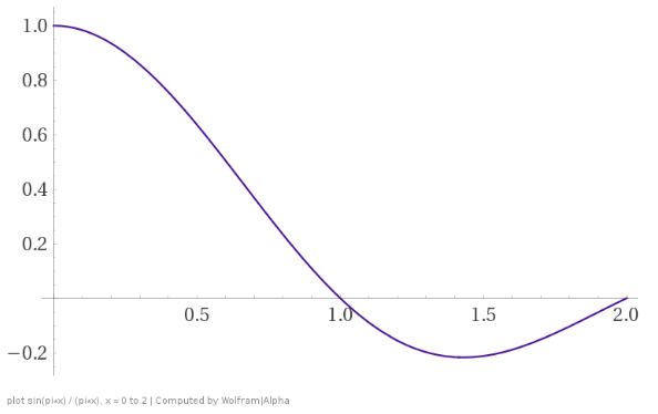
Figure 1: Plot of $\operatorname{sinc}\left({a}\right)=\sin\left(\pi a\right)/\left(\pi a\right)$, relating the displacement ($x$-axis) to the expected similarity ($y$-axis) between two unitary SPs. The similarity is symmetric about $a=0$.

Higher-Dimensional Spaces

To generalize this to SSPs representing $n$-dimensional space (e.g., $n=2$ in Komer et al. (2019)), we repeat the above recipe, where instead $\mathbf{X}\in\mathbb{R}^{n,d}$ and $\Theta\in\mathbb{R}^{n,d}$ are matrices, such that equations 1 and 2 hold for each row of $\mathbf{X}$ and $\Theta$. Now, with $\mathbf{x},\mathbf{a}\in\mathbb{R}^{n}$, equation 3 becomes:

$$A=\mathop{\scalebox{1.9}{\raisebox{-0.86108pt}{$\circledast$}}}_{k=1}^{n}{\mathbf{X}_{k}}^{x_{k}}\text{,}\quad B=\mathop{\scalebox{1.9}{\raisebox{-0.86108pt}{$\circledast$}}}_{k=1}^{n}{\vec{X}_{k}}^{x_{k}+a_{k}}\text{.}$$ (6)

Redoing equations 4 and 5 yields:

$$\boxed{A^{T}B=\frac{1}{d}\sum_{j=1}^{d}\text{Real}\left[\exp\left\{i\sum_{k=1}^{n}\Theta_{k,j}a_{k}\right\}\right]=\frac{1}{d}\sum_{j=1}^{d}\cos\left(\sum_{k=1}^{n}\Theta_{k,j}a_{k}\right)}\,\text{.}$$ (7)

Finally, for i.i.d. uniform $\Theta_{k,j}$, we obtain the following concrete equation for expected similarity:

$$\mathbb{E}_{\Theta}\left[A^{T}B\right]=\frac{1}{\left(2\pi\right)^{n}}\underbrace{\int_{-\pi}^{\pi}\cdots\int_{-\pi}^{\pi}}_{\text{$n$ integrals}}\cos\left(\sum_{k=1}^{n}\theta_{k}a_{k}\right)d\theta_{1}\cdots d\theta_{n}=\prod_{k=1}^{n}\sin\left(\pi a_{k}\right)/\left(\pi a_{k}\right)=\prod_{k=1}^{n}\operatorname{sinc}\left({a_{k}}\right)\text{.}$$ ∎

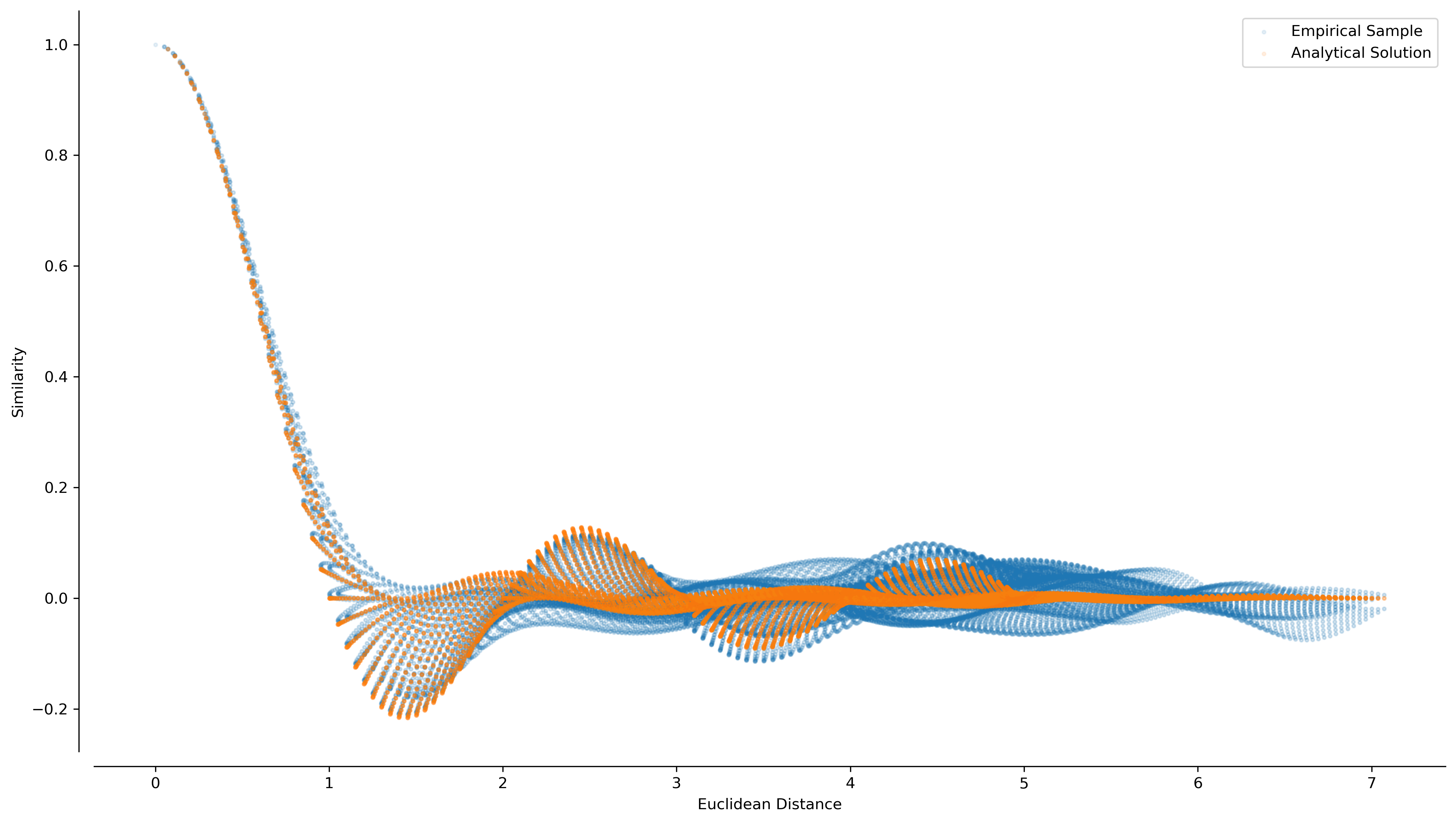
Figure 2: Empirical validation of our main result ($n=2$, $d=1024$). Two unitary vectors ($\mathbf{X}$) are randomly generated with uniformly distributed polar angles ($\Theta$), and the similarity is evaluated across a square grid of displacements, $\mathbf{a}\in[-5,5]^{2}$. For each displacement, we plot the Euclidean distance ($\|\mathbf{a}\|$) against the actual similarity ($A^{T}B$) in blue (empirical) as well as the expected similarity ($\prod_{k=1}^{n}\operatorname{sinc}\left({a_{k}}\right)=\prod_{k=1}^{n}\sin\left(\pi a_{k}\right)/\left(\pi a_{k}\right)$) in orange (analytical).

Figure 3: Surface plot of $\prod_{k=1}^{n}\operatorname{sinc}\left({a_{k}}\right)=\prod_{k=1}^{n}\sin\left(\pi a_{k}\right)/\left(\pi a_{k}\right)$ for $\mathbf{a}\in[-3,3]^{2}$, $n=2$, modelling the representation of an SSP encoding a two-dimensional point in space.

References

- Dumont and Eliasmith (2020) Nicole S-Y. Dumont and Chris Eliasmith. Accurate representation for spatial cognition using grid cells. In Proceedings of the 42nd Annual Meeting of the Cognitive Science Society., 2020.
- Gosmann (2018) Jan Gosmann. An Integrated Model of Context, Short-Term, and Long-Term Memory. Phd thesis, University of Waterloo, 2018. URL http://hdl.handle.net/10012/13498.
- Komer and Eliasmith (2020) Brent Komer and Chris Eliasmith. Efficient navigation using a scalable, biologically inspired spatial representation. In Proceedings of the 42nd Annual Meeting of the Cognitive Science Society., 2020.
- Komer et al. (2019) Brent Komer, Terrence C. Stewart, Aaron R. Voelker, and Chris Eliasmith. A neural representation of continuous space using fractional binding. In 41st Annual Meeting of the Cognitive Science Society, Montreal, QC, 2019. Cognitive Science Society.
- Plate (1995) Tony A Plate. Holographic reduced representations. IEEE Transactions on Neural Networks, 6(3):623–641, 1995.