NOH-NMS: Improving Pedestrian Detection by Nearby Objects Hallucination

Abstract.

Greedy-NMS inherently raises a dilemma, where a lower NMS threshold will potentially lead to a lower recall rate and a higher threshold introduces more false positives. This problem is more severe in pedestrian detection because the instance density varies more intensively. However, previous works on NMS don’t consider or vaguely consider the factor of the existent of nearby pedestrians. Thus, we propose Nearby Objects Hallucinator (NOH), which pinpoints the objects nearby each proposal with a Gaussian distribution, together with NOH-NMS, which dynamically eases the suppression for the space that might contain other objects with a high likelihood. Compared to Greedy-NMS, our method, as the state-of-the-art, improves by $3.9\%$ AP, $5.1\%$ Recall, and $0.8\%$ MR^-2 on CrowdHuman to $89.0\%$ AP and $92.9\%$ Recall, and $43.9\%$ MR^-2 respectively.

1. Introduction

Non-maximum Suppression (NMS) is widely used in proposal-based object detectors (Redmon et al., 2016; Redmon and Farhadi, 2017, 2018; Liu et al., 2016; Fu et al., 2017; Girshick et al., 2014; Girshick, 2015; Ren et al., 2015; Lin et al., 2017a; He et al., 2017; Cai and Vasconcelos, 2018; Dai et al., 2016, 2017; Lin et al., 2017b), as the post processing step to eliminate the redundant detections. Ideally, the proposal with the maximum score should suppress and only suppress all the other proposals of the same object. However, NMS distinguishes objects solely by a universal Intersection over Union (IoU) threshold. That is, if two proposals have an IoU above the pre-defined threshold, they will be considered as detecting the same object and one of them will be eliminated as the duplicate.

Figure 1. Comparison among various NMS methods The blue dotted box in (b) shows the mistakenly suppressed detection, which is caused by the NMS threshold dilemma in Greedy-NMS. The red dotted box in (c) highlights the false positive introduced by Adaptive-NMS as it is unable to pinpoint the overlapping areas. In order to recall the detection of the boy and suppress the red box, adapting the IoU threshold is not enough since $iou(box_{red},box_{green})<iou(box_{blue},box_{green})$, and NOH is designed for filling this gap.

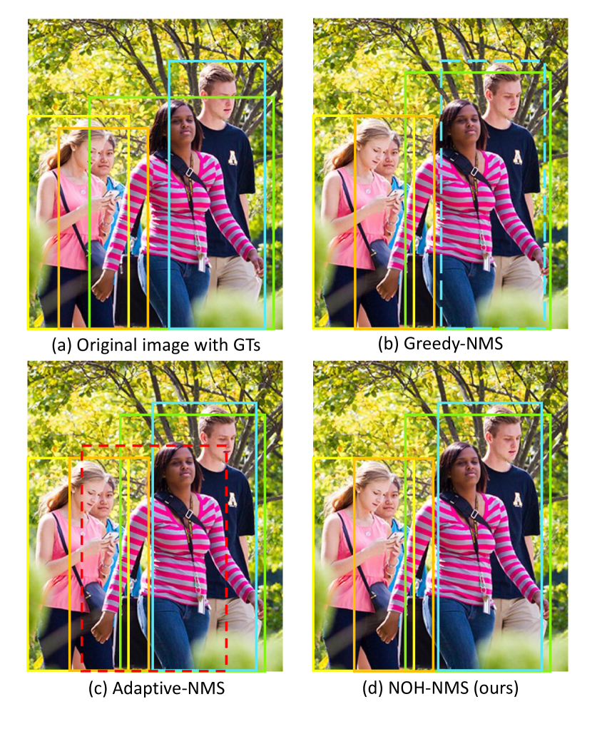
This scheme works fine in generic object detection task. However, it raises a dilemma in pedestrian detection task where the object density varies a lot, making it infeasible to find a perfect universal IoU threshold as a higher threshold fits for the regions with higher density and the less crowded regions desire a lower threshold (See Fig. 1).

Previous work tries to address this issue of the rigid NMS threshold. Soft-NMS (Bodla et al., 2017) proposes to degrade the score of nearby highly overlapped proposals instead of eliminating them, but just like Greedy-NMS, it still blindly penalizes the highly overlapped boxes. Adaptive-NMS (Liu et al., 2019) suggests directly predicting a proper NMS threshold for each proposal. However, even though the proposal can sense the density of the nearby objects, it is not aware of the locations and spread of the crowded regions, which results in a new dilemma, as shown in Fig. 1, where the left to the proposal is not dense at all and the right is rather crowded.

Thus, to tackle this problem, we propose Nearby Objects Hallucinator (NOH) and NOH-NMS. Our key observation is, in a crowded scene, the visual information inside a bounding box of one pedestrian will mostly contain the cues of the locations and sizes of other pedestrians. Therefore, we design NOH, which hallucinates the objects nearby each proposal based on the Region-of-Interest (RoI) feature and represents the hallucination with a Gaussian distribution. Furthermore, we propose NOH-NMS to perform a novel NMS strategy leveraging the Gaussian distribution.

The proposed NOH and NOH-NMS can be integrated naturally into both one-stage and two-stage object detectors with marginal computation cost and acquire no more extra annotations other than the full-body bounding boxes during training.

To evaluate the effectiveness of our method, we have conducted quantitative and qualitative experiments on CityPersons (Zhang et al., 2017) and CrowdHuman (Shao et al., 2018) datasets (see Sec. 4). As a result, we achieve state-of-the-art performance with $89.0\%$ AP, $92.9\%$ Recall, $43.9\%$ MR^-2 on CrowdHuman, and $10.8\%$ MR^-2 on CityPersons.

Our contributions can be summarized as follow:

• We propose NOH-NMS, which is aware of the existence of other nearby objects when performing the suppression, to address the rigid NMS threshold problem in pedestrian detection.

• We design NOH to pinpoint the objects nearby each proposal with a Gaussian distribution.

• Our method achieves state-of-the-art performance on CityPersons and Crowdhuman with negligible overhead.

2. Related Work

Over the past decade, deep convolutional neural networks (CNNs) have made great strides in image recognition (He et al., 2016). To adapt an image classifier into an object detector, the current common practice, called proposal-based object detector, leverages sliding window to densely predict, for each proposal, a set of category confidence scores and proposal refinement coefficients. These refined proposals are then fed into the NMS algorithm to get rid of the redundant detections. According to different strategies to generate the proposals, proposal-based object detectors can be classified into one-stage, where proposals are pre-defined anchors, and two-stage, where Region Proposal Networks (RPNs) are used for proposal generation. In addition, great progress has been made in multiple scaling (Lin et al., 2017a; Liu et al., 2018b), learnable anchors (Wang et al., 2019; Yang et al., 2018), deformable feature sampling (Dai et al., 2017; Zhu et al., 2019), etc.

Even though state-of-the-art generic object detectors show promising performance on benchmark datasets, such as COCO (Lin et al., 2014) and Pascal VOC (Everingham et al., 2015), it is non-trivial to adapt them into the pedestrian detection task, because the occlusion is much more severe and frequent in pedestrian detection datasets.

Occlusion can be divided into two categories, namely inter-class occlusion and intra-class occlusion. In intra-class occlusion scenarios, the pedestrian is occluded by other pedestrians. And the inter-class occlusion results in the partially visible feature of pedestrians mixed with the feature of background objects.

To address the problem of inter-class occlusion, some algorithms (Zhou and Yuan, 2018; Pang et al., 2019; Zhang et al., 2018) seek to leverage the annotated visible bounding box (VBB). (Zhou and Yuan, 2018) introduces a visible part estimation branch and a new training sample selecting strategy assisted by VBB. OR-CNN (Zhang et al., 2018) exploits the topological structure of the pedestrian with visibility prediction for occluded pedestrian detection. To emphasize on visible pedestrian regions during feature extraction, MGAN (Pang et al., 2019) proposes an attention module supervised by VBB.

In intra-class occlusion scenarios, the pedestrian is occluded by other pedestrians, which occurs frequently in the crowd scene. The heavily occluded between pedestrians confuses the models as it’s hard to distinguish instance boundaries. To alleviate this problem, OR-CNN (Zhang et al., 2018) designs aggregation loss to enforce generating more compact bounding boxes. In addition, RepLoss (Wang et al., 2018) proposes a novel repulsion loss to prevent the proposal from shifting to surrounding objects.

Though OR-CNN (Zhang et al., 2018) and RepLoss (Wang et al., 2018) successfully ease the localization problem in the crowded scenes, there still exists an even worse issue during the post-processing stage. In the post-processing stage, Non-maximum Suppression (NMS) is wildly used to suppress false positive proposals (i.e., the redundant pedestrian proposals belong to the same identity). However, NMS may also suppress true positive proposals (i.e., the highly overlapped pedestrian proposals belong to different identities). Therefore, a lower threshold leads to a lower Recall while a higher threshold results in lower precision.

To address this dilemma,  (Bodla et al., 2017) proposes Soft-NMS to replace the elimination operation with decaying the detection scores according to the IoU. And (Zhang et al., 2019; Chi et al., 2019) suggest using additional annotated head bounding boxes to solve the problem of NMS in a crowd, as the head parts usually suffer less from occlusion. More recently, Adaptive-NMS (Liu et al., 2019) proposes to predict the adaptive IoU threshold in NMS for each proposal. It aims at predicting a higher NMS threshold if the objects gather together and occlude each other, and predicting lower NMS threshold if the objects are sparse. However, even though Adaptive-NMS could predict accurate density for each proposal, a density scalar is not enough to precisely express the spatial locations of the crowded areas. In other words, the proposal is capable of sensing how crowded its surrounding is, but cannot tell if the area to its left is more crowded than the area to its right. As a result, Adaptive-NMS gets stuck into a new dilemma when different spatial locations to one object desire different IoU thresholds, as shown in Fig.1.

We observe this inflexibility in Adaptive-NMS and thus propose NOH and NOH-NMS to address this problem. Specifically, for NOH, we design a mini 2-fc branch to predict, for each proposal, not only a density scalar but also a Gaussian distribution which highlights the surrounding objects. In addition, our NOH-NMS leverages the output from NOH as the auxiliary information, together with the normal NMS input (detection boxes with class confidence), to perform a nearby-objects-aware NMS.

3. Our Method

In this section, we first briefly recap the previous NMS algorithms (Sec. 3.1). Then we propose our NOH-NMS which integrates the nearby-objects distribution into the NMS pipeline (Sec. 3.2). In addition, we illustrate how our NOH module learns to predict the nearby-objects distribution just from the box-level supervision (Sec. 3.3). Finally, we compare our method with the state-of-the-art NMS counterparts in with visualization (Sec. 3.4).

Input :  $\mathcal{B}={b_{1},\dots,b_{N}},\mathcal{S}={s_{1},\dots,s_{N}},$
$\mathcal{D}={d_{1},\dots,d_{N}},\mathcal{P}={p_{1},\dots,p_{N}},N_{t}$
$\mathcal{B}$ is the list of initial detection boxes
$\mathcal{S}$ contains corresponding detection scores
$\mathcal{D}$ contains corresponding detection densities
$\mathcal{P}$ contains the parameters of nearby-objects distribution of corresponding detection
$N_{t}$ is the NMS threshold

begin

       $\mathcal{F}\leftarrow\{\}$

       while $\mathcal{B}\neq empty$ do

             $m\leftarrow\text{argmax }\mathcal{S}$

             $\mathcal{M}\leftarrow b_{m}$

             $\mathcal{F}\leftarrow\mathcal{F}\bigcup\mathcal{M};\mathcal{B}\leftarrow\mathcal{B}-\mathcal{M}$

             for $b_{i}\in\mathcal{B}$ do

                   if iou$(\mathcal{M},b_{i})\geq N_{t}$ then

                        

                        

                        

                        

                        

                        

                   end if

                  

             end for

            

       end while

      return $\mathcal{F},\mathcal{S}$

end

Algorithm 1 Algorithm pseudo code NOH-NMS replaces the pruning step (highlighted in red) in Greedy-NMS with a nearby-objects-aware re-scoring function (marked with green).

3.1. Background

A proposal-based object detection framework consists of the following five stages: (1) extracting full-image-level feature; (2) generating bounding box proposals; (3) extracting proposal-region-level feature; (4) performing classification and box regression for each proposal; (5) removing redundant detections. In this pipeline, the proposals are usually densely arranged and there is no punishment if two or more detections are detecting the same object. Thus, prior to stage 5, it is rather common that one object area is occupied with multiple detections whereas only one of them counts towards true positive, and the rest are considered as false positive.

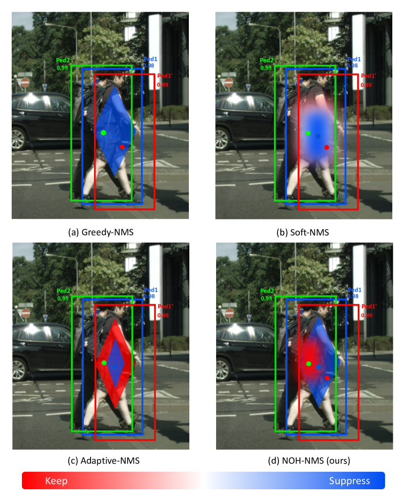
To avoid the aforementioned problem, Greedy-NMS selects the detection with the maximum score $\mathcal{M}$ and eliminates its surrounding inferior detections whose IoU with $\mathcal{M}$ is above certain threshold $N_{t}$, and then repeats this pruning process with the next best detection, as shown in Fig. 1. The pruning step, as the core of the NMS algorithm, can be formulated into a re-scoring function as follow:

(1) $$s_{i}=\left\{\begin{array}[]{ll}s_{i},&\text{iou}(\mathcal{M},b_{i})<N_{t}\\ 0,&\text{iou}(\mathcal{M},b_{i})\geq N_{t}\end{array},\right.$$

where $s_{i}$ and $b_{i}$ denote the confidence score and bounding box coefficients of the inferior detections. $b_{i}$ will be either left unmodified or completely removed depending solely on its IoU with $\mathcal{M}$. This introduces two problems. (1) The consequence is too extreme and IoU, as the only metric, is not robust enough, which makes the performance very sensitive to the choice of the NMS threshold. E.g., when $N_{t}$ is set to $0.5$, detection $b_{i}$ will be eliminated if iou$(\mathcal{M},b_{i})$ equals to $0.51$, however, with a slight perturbation, iou$(\mathcal{M},b_{i})$ could become $0.49$, which makes $b_{i}$ survive. (2) There is no such NMS threshold that makes everyone happy. E.g., an image occupied with $100$ objects might desire $0.3$ as the threshold, while it is not suitable for the image with a single object.

In response to the first problem, Soft-NMS softens the consequence by gradually decaying the score of the overlapped detections instead of eliminating them. Below shows its re-scoring function:

(2) $$s_{i}=\left\{\begin{array}[]{ll}s_{i},&\text{iou}(\mathcal{M},b_{i})<N_{t}\\ s_{i}\cdot f(\mathcal{M},b_{i}),&\text{iou}(\mathcal{M},b_{i})\geq N_{t}\end{array},\right.$$

where decaying function $f$ is chosen to be:

(3) $$f(\mathcal{M},b_{i})=1-\text{iou}(\mathcal{M},b_{i})\;\;\textbf{or}\;\;\text{exp}(-\text{iou}(\mathcal{M},b_{i})^{2}/\sigma)$$

For the second problem, Adaptive-NMS customizes an NMS IoU threshold for each proposal and follows the design of Greedy-NMS except now the IoU threshold $N_{\mathcal{M}}$ varies with the current best detection $\mathcal{M}$. Their strategy can be formulated as:

(4) $$N_{\mathcal{M}}:=\text{max}(N_{t},d_{\mathcal{M}}),$$

(7) $$s_{i}=\left\{\begin{array}[]{ll}s_{i},&\text{iou}(\mathcal{M},b_{i})<N_{\mathcal{M}}\\ 0,&\text{iou}(\mathcal{M},b_{i})\geq N_{\mathcal{M}}\end{array},\right.$$

where $d_{\mathcal{M}}$ is the density prediction of proposal $\mathcal{M}$.

As we carefully re-visit Adaptive-NMS, we find that due to the maximum function, Adaptive-NMS can be re-written into a super case of Soft-NMS:

(8) $$s_{i}=\left\{\begin{array}[]{ll}s_{i},&\text{iou}(\mathcal{M},b_{i})<N_{t}\\ s_{i}\cdot f(\mathcal{M},b_{i},d_{\mathcal{M}}),&\text{iou}(\mathcal{M},b_{i})\geq N_{t}\end{array},\right.$$

where

(9) $$f(\mathcal{M},b_{i},d_{\mathcal{M}})=\left\{\begin{array}[]{ll}1,&\text{iou}(\mathcal{M},b_{i})<d_{\mathcal{M}}\\ 0,&\text{iou}(\mathcal{M},b_{i})\geq d_{\mathcal{M}}\end{array}\right.$$

As shown in Eq. 2 and Eq. 8, compared to Greedy-NMS, Soft-NMS adds the location of $b_{i}$ into consideration when suppressing $b_{i}$ and Adaptive-NMS further considers the density of $\mathcal{M}$. However, both of them cannot accurately distinguish whether $b_{i}$ is detecting a nearby object or $b_{i}$ is a false positive. Although equipped with density prediction, Adaptive-NMS still cannot tell where the objects around $\mathcal{M}$ are, let alone Soft-NMS.

3.2. NOH-NMS

The key idea of our NOH-NMS is to introduce the nearby-objects distribution $P_{p_{\mathcal{M}}}$ into the NMS pipeline, where $p_{\mathcal{M}}$ denotes its parameters. The nearby-objects distribution could be obtained by any probability distribution functions (PDFs), and we will cover our choice of generating $P_{p_{\mathcal{M}}}$ in Sec. 3.3. Note that, in the pedestrian detection task, the only object category we care is human, therefore the nearby objects refer to nearby pedestrians mostly in this paper. However, our method can also be used in other tasks where the nearby objects won’t be limited to humans only.

Figure 2. Architecture The illustration of integrating Nearby Objects Hallucinator (NOH) into the two-stage object detector, such as Faster-RCNN (Ren et al., 2015). Note that our NOH can fit in single-stage object detectors as well by placing the NOH branch in parallel with the detection head. In this example, the lady at the front left is highly overlapped with the lady behind her, and our NOH pinpoints the location and shape of the lady behind so that the detection of her won’t be mistakenly suppressed whereas other false positives will be eliminated.

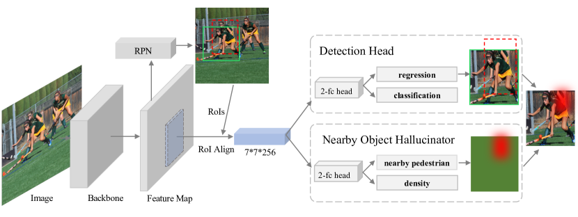
NOH-NMS consists of two components, namely overlap detector and NOH-Suppressor.

Overlap Detector Since our assumption is that the bounding box area of one pedestrian will mostly contain the cues of other pedestrians, we need to first rule out the cases where the cues are not abundant (e.g. a pedestrian is by its alone). Thus, we propose a simple overlap detector, which predicts the IoU between the $\mathcal{M}$ and the object overlapped with $\mathcal{M}$ the most. If the predicted IoU is less than a threshold $d_{t}$, which we empirically set to $0.3$, then NOH-Suppressor won’t be triggered because of insufficient cues, and we will follow the design of Greedy-NMS ($s_{i}:=0$) or Soft-NMS ($s_{i}:=s_{i}f(\text{iou}(\mathcal{M},b_{i}))$).

NOH-Suppressor If the cues are predicted to be sufficient, we will perform NOH-Suppression, which re-scores the $s_{i}$ by multiplying the probability of $b_{i}$ being a nearby object. In this way, when a neighboring box meets the attributes of being a nearby object, the suppression on it will be dynamically eased, whereas if it is very unlikely to be a nearby object, then we treat it as detecting the same object of $\mathcal{M}$, which should be degraded. We formally describe the difference between NOH-NMS and Greedy-NMS in Fig. 1. As we only replace the re-scoring function with a Gaussian function runs at $O(1)$, we haven’t introduced computational complexity into the NMS pipeline. In addition, since we leverage the mini 2-fc branch to predict both distribution parameters and density directly from RoI feature, the overhead is negligible (See Fig. 2).

In summary, the strategy we adopt can be described as follow:

(10) $$s_{i}=\left\{\begin{array}[]{ll}s_{i},&\text{iou}(\mathcal{M},b_{i})<N_{t}\\ s_{i}\cdot f(\mathcal{M},b_{i},d_{\mathcal{M}},p_{\mathcal{M}}),&\text{iou}(\mathcal{M},b_{i})\geq N_{t}\end{array},\right.$$

(11) $$f(\mathcal{M},b_{i},d_{\mathcal{M}},p_{\mathcal{M}})=\left\{\begin{array}[]{ll}P_{p_{\mathcal{M}}}(\mathcal{M},b_{i}),&d_{\mathcal{M}}\geq d_{t}\\ 0,&d_{\mathcal{M}}<d_{t}\end{array}\right.$$

Note that, if the step function in Eq. 9 is used as the PDF, then our NOH-NMS degenerates to Adaptive-NMS. However, the step function is rarely used for modeling the natural distributions because (1) it is not continuous, and (2) it is oversimplified. Thus, we propose NOH (Sec. 3.3) to better capture the true nearby-objects distribution using the Gaussian distribution.

3.3. Nearby Objects Hallucinator (NOH)

NOH is responsible for generating the nearby-objects distribution for each $\mathcal{M}$. We achieve this by hallucinating the locations and shapes of the nearby objects from the cues in region $\mathcal{M}$, and expressing the hallucination with a Gaussian distribution. We term this process as hallucination because different from proposal-based instance recognition, which predicts box coefficients from the proper RoI feature, our NOH could only rely on partially visible cues.

Essentially, based on the features extracted from region $\mathcal{M}$, multiple hallucination objects could be proposed. However, for simplicity, we only capture one nearby object which overlaps with $\mathcal{M}$ the most. We represent the hallucinated object with its relative center location, width, height with $\mathcal{M}$, denoted as $\mu_{\mathcal{M}}$. Since the hallucinated object is predicted by partially visible cues, the prediction is expected to be imprecise. Thus, we decay the nearby-objects likelihood with a Gaussian distribution which centers at $\mu_{\mathcal{M}}$ and spreads with a hyper-parameter $\sigma$.

With all the definition above, our NOH applies the following strategy:

(12) $$P_{\mu_{\mathcal{M}}}(\mathcal{M},b_{i})=\text{exp}(-\left\lVert b_{i|\mathcal{M}}-\mu_{\mathcal{M}}\right\rVert^{2}/2\sigma^{2})$$

(13) $$b_{i|\mathcal{M}}=\{\frac{x_{b_{i}}-x_{\mathcal{M}}}{w_{\mathcal{M}}},\frac{y_{b_{i}}-y_{\mathcal{M}}}{h_{\mathcal{M}}},\text{log}\frac{w_{b_{i}}}{w_{\mathcal{M}}},\text{log}\frac{h_{b_{i}}}{h_{\mathcal{M}}}\}$$

Figure 3. Visualization of the suppression degree The suppression degree is a function of the relative center location and relative shape of two boxes, resulting in 4-d freedom. To visualize it in 2-d space, we unify the shapes of all the boxes so that each box can be represented by its center point. The detection score is attached to the corner of the box. The color map shows to what extent the detection with the maximum score (blue box) suppresses its surrounding inferior detections. For instance, the center point of the green box in (d) lies in the red area (keeping area), meaning it is very likely to survive the suppression, whereas the red box will be penalized harshly as its center sits in the blue area (suppressing area).

We implement NOH with a prediction head in parallel with the classification and regression head of Faster-RCNN. The training target of NOH is derived from the relative box coefficients of the most nearby object with $\mathcal{M}$, and we impose Smooth-L1 loss as the training loss. Note that, the Gaussian function is not represented during the training. However, we could convert the training target from the relative box coefficients into a Dirac delta function, and supervise it with KL Loss (He et al., 2019). In this paper, we keep the training process simple, as we find it works up to the expectation, and stick with the Smooth-L1 loss.

3.4. Comparisons with other NMS Strategies

To better understand the difference among NMS strategies that we and other methods propose, we visualize the suppression effect of $\mathcal{M}$ on overlapped other detections in Fig. 3. According to the figure, Greedy-NMS harshly eliminates the detections around $\mathcal{M}$, and Soft-NMS gradually adds keeping area. Adaptive-NMS, on the other hand, adds a more harsh keeping area, as the result of the usage of the step function, but the proportion of such area is adaptive to the pedestrian density. Note that when combining Soft-NMS and Adaptive-NMS together, the keeping area will be both continuous and adaptive. However, all the aforementioned methods cannot shift the center of the keeping area because they don’t explicitly predict the distribution of the nearby pedestrians, whereas our method places the keeping area more accurate thanks to the NOH module.

4. Experiments

In this section, we first cover the datasets and metrics that we use for all the experiments (Sec. 4.1). We then reveal our implementation details in Sec. 4.2 and show quantitative results of NOH-NMS compared to various NMS methods (Sec. 4.3). We also conduct sensitivity analysis (Sec. 4.4) to prove the robustness of our method. Qualitative results are also prepared in Sec. 4.5 for better visualization.

4.1. Datasets and Metrics

CityPersons CityPersons (Zhang et al., 2017) is a currently wildly used benchmark dataset in the pedestrian detection task. Based on the $5000$ images in the Cityscapes (Cordts et al., 2016) dataset, CityPersons creates more fine-grained bounding box annotations which dedicate to pedestrian detection. In total, CityPersons covers $\sim 35$k person and $\sim 13k$ ignore region (fake humans like statues) annotations. In addition, CityPersons aims at including persons with heavy occlusion and small scale, yielding an average density of $\sim 7$ persons per image.

CrowdHuman CrowdHuman (Shao et al., 2018) was released more recently, which further emphasizes the crowd issue. It contains $15,000$ images, with $\sim 340$k person and $\sim 99$k ignore region annotations. The person density is significantly higher than CityPersons and reaches $\sim 22.6$ persons per image with $2.4$ pairwise overlapping instances (IoU larger than $0.5$).

Evaluation metrics We follow the evaluation metrics used in CityPersons and CrowdHuman, denotes as MR^-2, AP, and Recall:

• MR^-2, or log-average Miss Rate on False Positive Per Image (FPPI) in $[10^{-2},10^{0}]$, is commonly used to evaluate detectors whose applications have an upper limit on the acceptable FPPI rate independent of object density. Thus, MR^-2 is particularly sensitive to false positives.

• Average Precision (AP) is the most popular metric in generic object detection, which summarizes the precision-recall curve of the detection results. In the following experiments, we follow the AP metric in PASCAL VOC (Everingham et al., 2015), where a prediction is positive if IoU $\geq 0.5$.

• Recall is short for the maximum recall given a fixed number of detections. As both Soft-NMS, Adaptive-NMS, and NOH-NMS aim at recalling the mis-eliminated true positives, as shown in Fig .3, this metric reflects the effectiveness of this intention. For fair comparisons, we set the allowed number of detections to be $100$ for all NMS methods.

Methods	Extra Anno.	Backbone	Scale	Reasonable	Bare	Partial	Heavy
OR-CNN (Zhang et al., 2018)	✓	VGG-16	$\times 1.3$	11.0	5.9	13.7	51.3
MGAN (Pang et al., 2019)	✓	VGG-16	$\times 1.3$	10.5	-	-	47.2
JointDet (Chi et al., 2019)	✓	ResNet-50	$\times 1.3$	10.2	-	-	-
TLL (MRF) (Song et al., 2018)		ResNet-50	-	14.4	-	-	-
Adapted Faster RCNN (Zhang et al., 2017)		VGG-16	$\times 1.3$	13.0	-	-	-
ALFNet (Liu et al., 2018a)		VGG-16	$\times 1$	12.0	8.4	11.4	51.9
RepLoss (Wang et al., 2018)		ResNet-50	$\times 1.3$	11.6	7.0	14.8	55.3
Adaptive-NMS w/ AggLoss (Liu et al., 2019)		VGG-16	$\times 1.3$	10.8	6.2	11.4	54.0
Our baseline		ResNet-50	$\times 1.3$	11.9	7.4	12.3	53.0
NOH-NMS		ResNet-50	$\times 1.3$	10.8	6.6	11.2	53.0

Table 1. Performance on the CityPersons validation set. MR^-2 is used as the metric (lower is better). Scale is short for input scale.

4.2. Implementation Details

For all the experiments, we adapt the Faster-RCNN (Ren et al., 2015) with FPN (Lin et al., 2017a) as our baseline and build various NMS methods upon the same baseline for fair comparisons. In specific, we choose the standard ResNet-50 (He et al., 2016) as the backbone and replace the ROIPooling operation in the original Faster-RCNN with the RoIAlign (He et al., 2017). We also change the aspect ratios of the anchors to $H/W=\{1,2,3\}$ for CrowdHuman and $H/W=\{2.44\}$ for CityPersons, as the original anchor settings are optimized towards COCO (Lin et al., 2014). Following the choice of input size in (Zhang et al., 2017) and (Shao et al., 2018), we enlarge the input height and width of CityPersons by $1.3$ times and resize the input of CrowdHuman so that the shorter edge of input equals to 800 pixels while keeping the longer edge no longer than 1,400 pixels.

During training, we randomly initialize all the parameters of the model by Kaiming initialization (He et al., 2015), except the ResNet-50 backbone, whose initial parameters are loaded from ImageNet (Russakovsky et al., 2015) pre-train. We use SGD with $0.9$ momentum and $0.0001$ weight decay as the optimizer and train the model with $5,600$ and $28,125$ iterations in total for CityPersons and CrowdHuman respectively. The initial learning rate is $0.02(0.04)$ and decreases by a factor of $10$ after $3,400(18,750)$ and $4,600(24,375)$ iterations for CityPersons (CrowdHuman). The batch size is set to be $16$ for both datasets. Note that we train on 8 GPUs without Synchronized BN.

For CityPersons, a sample will be assigned as positive if its IoU with ground-truth is greater than $0.7$, and as negative if the IoU is less than $0.5$, otherwise the sample will be ignored and won’t contribute to the loss. For CrowdHuman, samples with IoU greater than $0.5$ qualify as the positive and otherwise are considered as negative. In addition, we clip the ground-truth bounding boxes at the image boundary for CityPersons, while don’t apply this operation in CrowdHuman.

During inference, we set the NMS IoU threshold to $0.5$ for all NMS methods and allow at most $100$ detections per image. We also follow the same input resizing operation as mentioned in the training stage.

Methods	Backbone	AP	Recall	MR-2
Repulsion Loss (Wang et al., 2018)	R50	-	-	45.7
JointDet* (Chi et al., 2019)	R50	-	-	46.5
Baseline in (Liu et al., 2019)	R50	83.0	90.6	52.4
Adaptive-NMS (Liu et al., 2019)	R50	84.7	91.3	49.7
Our Baseline	R50	85.1	87.8	44.7
NOH-NMS	R50	89.0	92.9	43.9

Table 2. Performance on the CrowdHuman validation set. R50 denotes ResNet-50. * marks the methods which leverage extra annotations (e.g. head box) during training.

Methods	$N_{t}$	AP	Recall	$MR^{-2}$
Greedy-NMS	0.5	85.1	87.8	44.7
Soft-NMS (Bodla et al., 2017)	0.5	86.4	90.6	44.6
Adaptive-NMS (Liu et al., 2019)	0.5	87.1	89.2	45.0
NOH-NMS	0.5	89.0	92.9	43.9

Table 3. Comparison of different NMS methods on the CrowdHuman validation set. All the methods are implemented by us, and for fair comparisons, we show the best results from multiple runs.

4.3. Results

CityPersons We report the results of NOH-NMS and other state-of-the-art pedestrian detectors on CityPersons validation set in Tab. 1. In particular, according to the level of occlusion, the CityPersons has four splits, namely Bare, Partial, Reasonable, and Heavy, whose ratios of visible parts are $[0.9,1],[0.65,0.9],[0.65,1],[0.2,0.65]$. Within the group of the methods which don’t use extra annotation, NOH-NMS achieves the best performance on Reasonable, which is the most valued, and Partial splits. Moreover, our performance is comparable to that of the methods using additional annotations (e.g. head bounding boxes, visible bounding boxes).

CrowdHuman Tab. 2 shows the performance on CrowdHuman validation set. To have a comprehensive evaluation, three evaluation metrics are chosen to evaluate our method, which are AP, Recall, and MR^-2. We re-implement a strong FPN (Lin et al., 2017a) baseline. Our baseline achieves $85.1\%$ AP, $87.8\%$ Recall and $44.7\%$ MR^-2, which outperforms the baseline in Adaptive-NMS (Liu et al., 2019) by $0.4\%$ AP and $5.0\%$ MR^-2. Although compared to our strong Greedy-NMS baseline, NOH-NMS still significantly improves the AP, Recall, and MR^-2 by $3.9\%$, $5.1\%$, and $0.8\%$. Moreover, compared to other state-of-the-art methods, superior performance demonstrates the effectiveness of our method.

To better demonstrate that our performance gain is not from the strong baseline, and show more clearly the advantage of NOH-NMS compared with its counterparts, we re-implement Soft-NMS and Adaptive-NMS on our strong baseline. The results are shown in Tab. 3. According to the results, NOH-NMS still delivers the best performance across all the evaluation metrics.

Figure 4. Precision vs. Recall at multiple NMS IoU thresholds $\mathbf{N_{t}}$ Experiments are conducted on the CrowdHuman validation set and all the NMS methods are implemented by us based on the same baseline.

Figure 5. Sensitivity to hyper-parameters We show the effect of the different choices of $\sigma$ and $d_{t}$ on NOH-NMS. All the experiments are done on the CrowdHuman validation set.

4.4. Sensitivity Analysis

Although NOH-NMS introduces two more hyper-parameters (density threshold $d_{t}$ and Gaussian standard deviation $\sigma$) than the other NMS methods, as we analyze later, it is not only robust to the choice of $d_{t}$ and $\sigma$, but also less sensitive to the common hyper-parameter $N_{t}$ than other NMS.

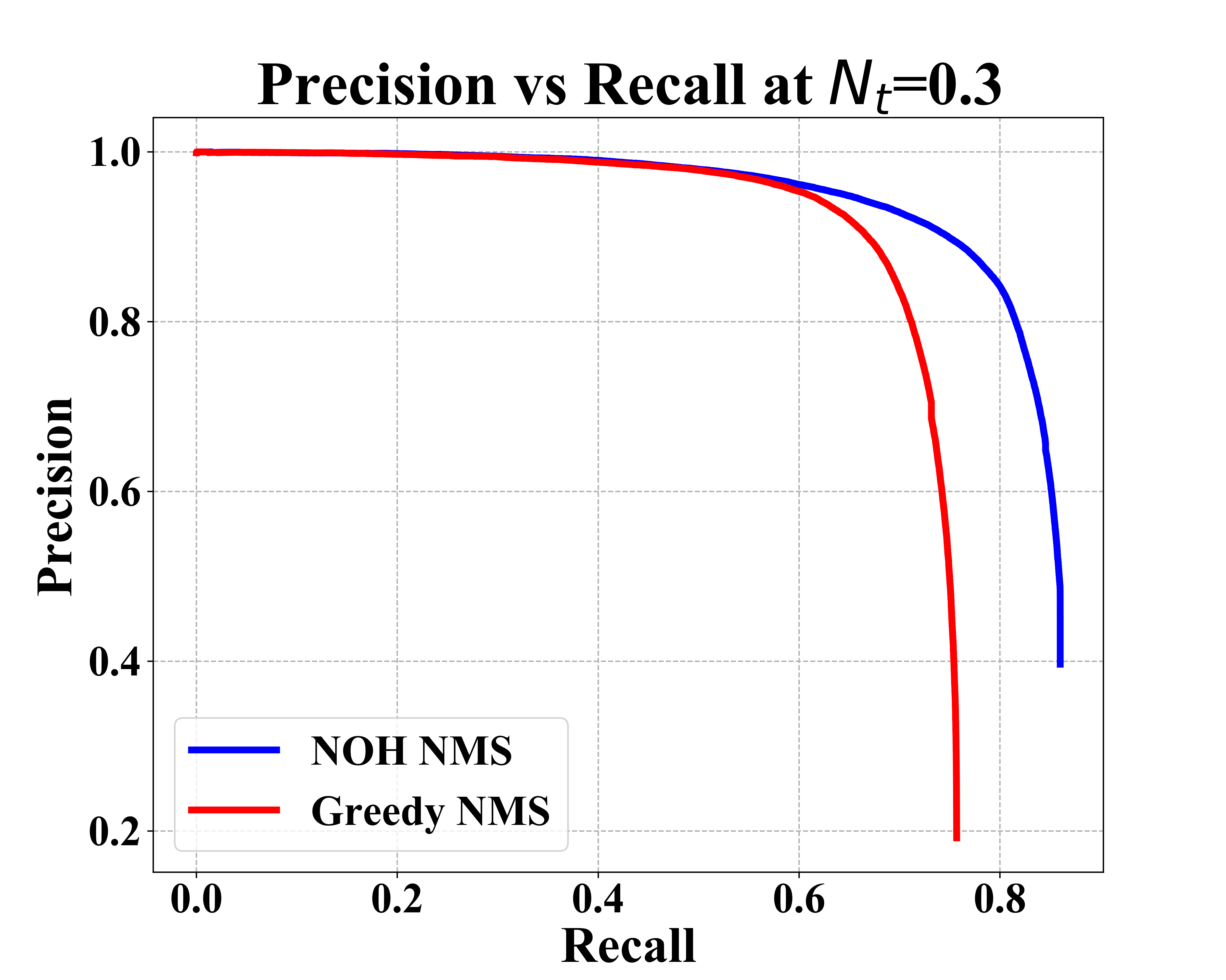
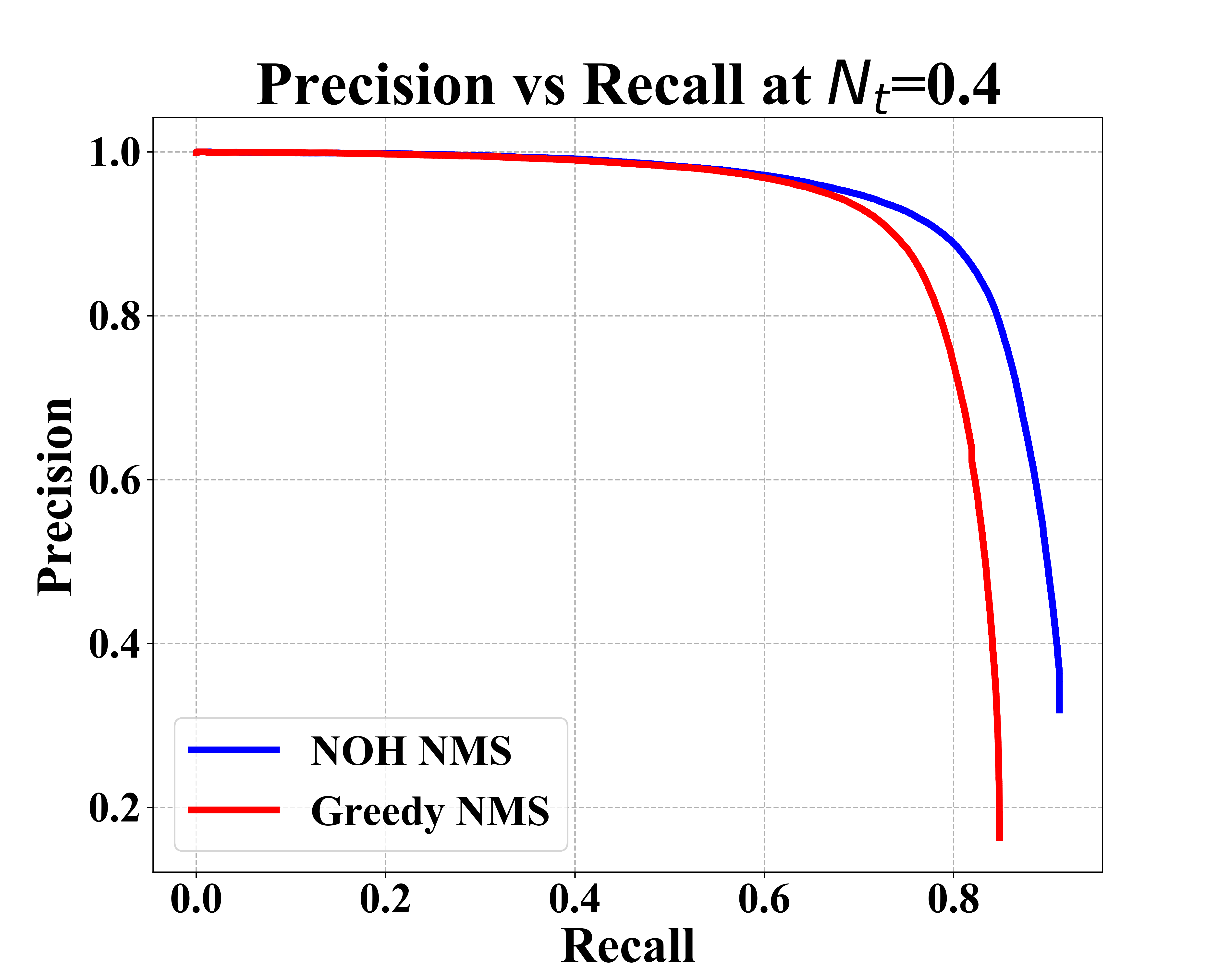
IoU threshold As shown in Fig. 4, we plot the precision vs. recall curves on various NMS IoU thresholds for both Greedy-NMS and NOH-NMS. We conclude two points from the figure. (1) Even though both methods degrade with sub-optimal IoU threshold hyper-parameter, NOH-NMS is less sensitive as it outperforms the Greedy-NMS in all recall levels across all the choice of $N_{t}$. (2) Simply flexing the IoU threshold for Greedy-NMS does recall more true positives but also introduces even more false positives that overwhelm the overall performance.

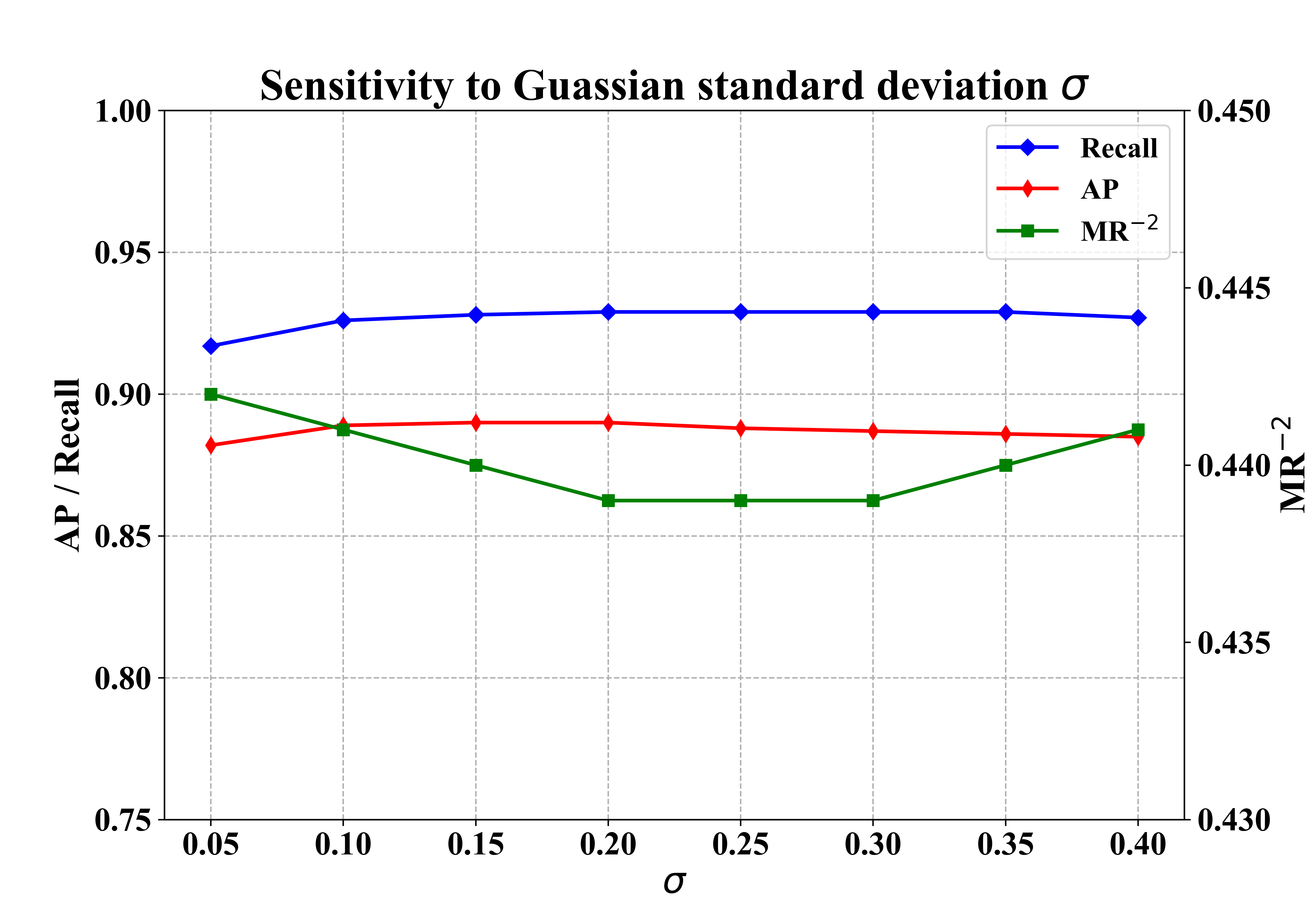
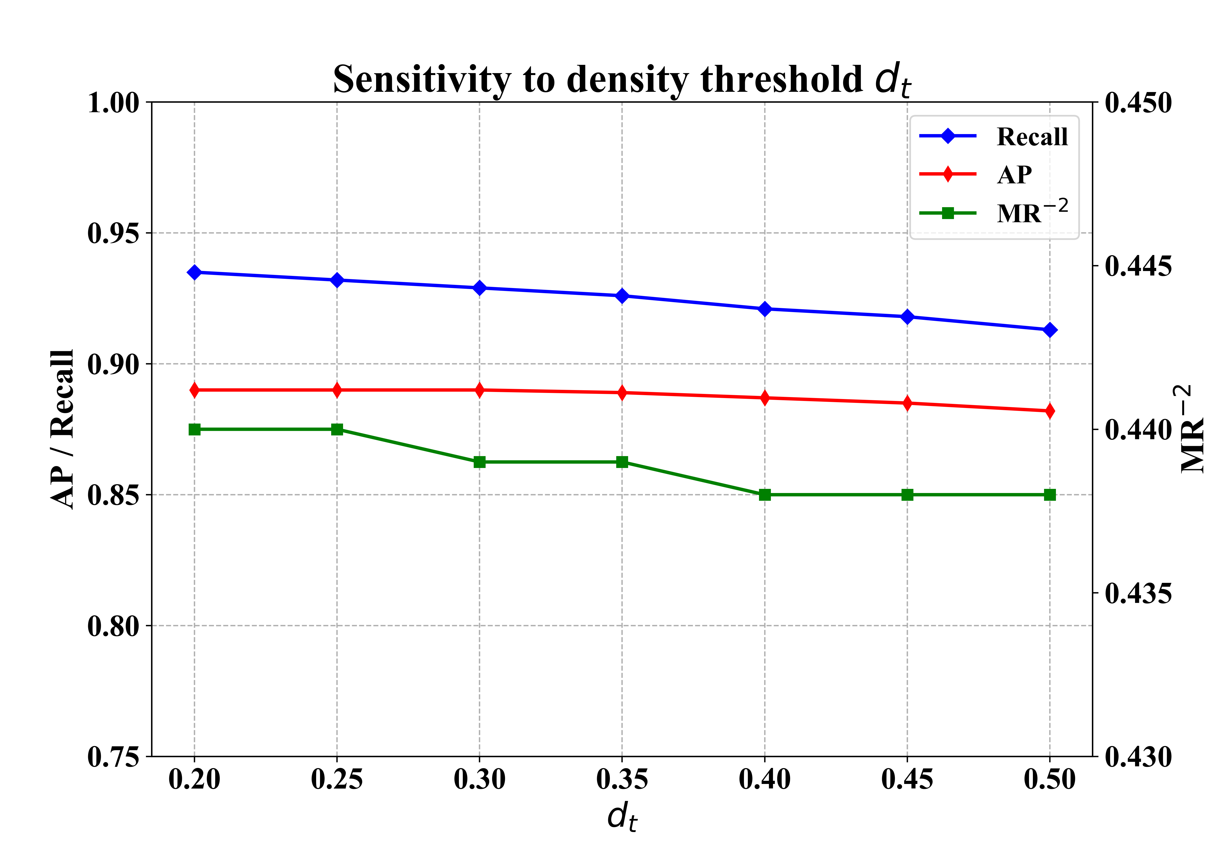
Density threshold As one of the additional hyper-parameters we introduce, the density threshold $d_{t}$ determines what it takes to be considered as having abundant cues to support the existence of other nearby pedestrians. As shown in Fig. 5, the performance for AP, recall, and MR^-2 jitters slightly with a wild range of $d_{t}$ (from $0.2$ to $0.5$ with an interval of $0.05$), which proves the robustness of NOH-NMS.

Gaussian standard deviation $\sigma$ controls the spread of the Gaussian distribution we use in NOH. Even though we empirically set it to $0.2$ in our previous experiments, it is proven to be not very sensitive as illustrated in Fig. 5. Note that, if using KL Loss during training, the $\sigma$ can be trained end-to-end, and will no longer be a hyper-parameter. However, we leave this as future work since it is not the focus of this paper.

4.5. Qualitative Results

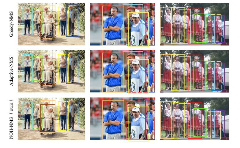
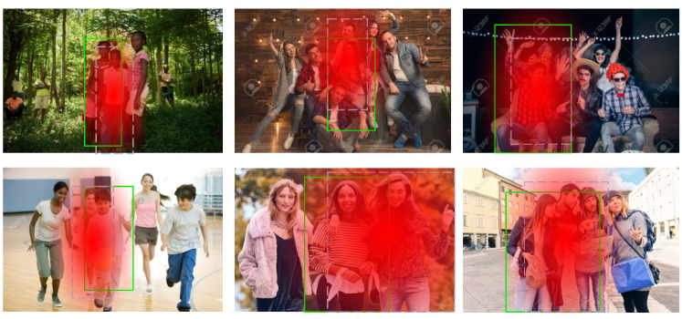
Qualitative results are given in two aspects: (1) detections visualization compared with Greedy-NMS and Adaptive-NMS (Fig. 6); (2) illustration of the effectiveness of the nearby objects hallucination (Fig. 7).

As shown in Fig. 6, our NOH-NMS successfully recalls the highly overlapped detections that other methods fail to do so. Moreover, in Fig. 7, the Nearby Objects Hallucinator works as expect, pinpointing the nearby persons with a reasonable Gaussian distribution, which contributes significantly to helping NOH-NMS ease the suppression on the highly overlapped areas.

5. Conclusion

In this paper, we present a novel NOH-NMS algorithm that improves the performance of pedestrian detection by taking into account the distribution of nearby objects. As the core part of our algorithm, Nearby Objects Hallucinator learns to predict the Gaussian distribution of nearby objects from only full-body box annotations and introduces marginal overhead. Comprehensive experiments and analyses are done on CityPersons (Zhang et al., 2017) and CrowdHuman (Shao et al., 2018) to show the strength of NOH-NMS.

Figure 6. Qualitative results Evaluation results on the CrowdHuman validation set. The NMS IoU threshold is set to $0.5$ for all the methods. The dotted boxes show the missing detections.

Figure 7. The visualization of the nearby objects hallucination results NOH models the distribution of nearby objects with a 4-d Gaussian whose mean $\mu_{\mathcal{M}}$ represents the expectation of the location and shape of the nearest object (shown in the dotted blue box). The variance of the 2-d transition of the center points is illustrated in red (we don’t show the shape variance). The green boxes show the prediction for $\mathcal{M}$.

References

- (1)
- Bodla et al. (2017) Navaneeth Bodla, Bharat Singh, Rama Chellappa, and Larry S Davis. 2017. Soft-NMS–improving object detection with one line of code. In Proceedings of the IEEE international conference on computer vision. 5561–5569.
- Cai and Vasconcelos (2018) Zhaowei Cai and Nuno Vasconcelos. 2018. Cascade r-cnn: Delving into high quality object detection. In Proceedings of the IEEE conference on computer vision and pattern recognition. 6154–6162.
- Chi et al. (2019) Cheng Chi, Shifeng Zhang, Junliang Xing, Zhen Lei, Stan Z Li, and Xudong Zou. 2019. Relational Learning for Joint Head and Human Detection. arXiv preprint arXiv:1909.10674 (2019).
- Cordts et al. (2016) Marius Cordts, Mohamed Omran, Sebastian Ramos, Timo Rehfeld, Markus Enzweiler, Rodrigo Benenson, Uwe Franke, Stefan Roth, and Bernt Schiele. 2016. The cityscapes dataset for semantic urban scene understanding. In Proceedings of the IEEE conference on computer vision and pattern recognition. 3213–3223.
- Dai et al. (2016) Jifeng Dai, Yi Li, Kaiming He, and Jian Sun. 2016. R-fcn: Object detection via region-based fully convolutional networks. In Advances in neural information processing systems. 379–387.
- Dai et al. (2017) Jifeng Dai, Haozhi Qi, Yuwen Xiong, Yi Li, Guodong Zhang, Han Hu, and Yichen Wei. 2017. Deformable convolutional networks. In Proceedings of the IEEE international conference on computer vision. 764–773.
- Everingham et al. (2015) Mark Everingham, SM Ali Eslami, Luc Van Gool, Christopher KI Williams, John Winn, and Andrew Zisserman. 2015. The pascal visual object classes challenge: A retrospective. International journal of computer vision 111, 1 (2015), 98–136.
- Fu et al. (2017) Cheng-Yang Fu, Wei Liu, Ananth Ranga, Ambrish Tyagi, and Alexander C Berg. 2017. Dssd: Deconvolutional single shot detector. arXiv preprint arXiv:1701.06659 (2017).
- Girshick (2015) Ross Girshick. 2015. Fast r-cnn. In Proceedings of the IEEE international conference on computer vision. 1440–1448.
- Girshick et al. (2014) Ross Girshick, Jeff Donahue, Trevor Darrell, and Jitendra Malik. 2014. Rich feature hierarchies for accurate object detection and semantic segmentation. In Proceedings of the IEEE conference on computer vision and pattern recognition. 580–587.
- He et al. (2017) Kaiming He, Georgia Gkioxari, Piotr Dollár, and Ross Girshick. 2017. Mask r-cnn. In Proceedings of the IEEE international conference on computer vision. 2961–2969.
- He et al. (2015) Kaiming He, Xiangyu Zhang, Shaoqing Ren, and Jian Sun. 2015. Delving deep into rectifiers: Surpassing human-level performance on imagenet classification. In Proceedings of the IEEE international conference on computer vision. 1026–1034.
- He et al. (2016) Kaiming He, Xiangyu Zhang, Shaoqing Ren, and Jian Sun. 2016. Deep residual learning for image recognition. In Proceedings of the IEEE conference on computer vision and pattern recognition. 770–778.
- He et al. (2019) Yihui He, Chenchen Zhu, Jianren Wang, Marios Savvides, and Xiangyu Zhang. 2019. Bounding box regression with uncertainty for accurate object detection. In Proceedings of the IEEE Conference on Computer Vision and Pattern Recognition. 2888–2897.
- Lin et al. (2017a) Tsung-Yi Lin, Piotr Dollár, Ross Girshick, Kaiming He, Bharath Hariharan, and Serge Belongie. 2017a. Feature pyramid networks for object detection. In Proceedings of the IEEE conference on computer vision and pattern recognition. 2117–2125.
- Lin et al. (2017b) Tsung-Yi Lin, Priya Goyal, Ross Girshick, Kaiming He, and Piotr Dollár. 2017b. Focal loss for dense object detection. In Proceedings of the IEEE international conference on computer vision. 2980–2988.
- Lin et al. (2014) Tsung-Yi Lin, Michael Maire, Serge Belongie, James Hays, Pietro Perona, Deva Ramanan, Piotr Dollár, and C Lawrence Zitnick. 2014. Microsoft coco: Common objects in context. In European conference on computer vision. Springer, 740–755.
- Liu et al. (2019) Songtao Liu, Di Huang, and Yunhong Wang. 2019. Adaptive nms: Refining pedestrian detection in a crowd. In Proceedings of the IEEE Conference on Computer Vision and Pattern Recognition. 6459–6468.
- Liu et al. (2018b) Shu Liu, Lu Qi, Haifang Qin, Jianping Shi, and Jiaya Jia. 2018b. Path Aggregation Network for Instance Segmentation. In Proceedings of IEEE Conference on Computer Vision and Pattern Recognition (CVPR).
- Liu et al. (2016) Wei Liu, Dragomir Anguelov, Dumitru Erhan, Christian Szegedy, Scott Reed, Cheng-Yang Fu, and Alexander C Berg. 2016. Ssd: Single shot multibox detector. In European conference on computer vision. Springer, 21–37.
- Liu et al. (2018a) Wei Liu, Shengcai Liao, Weidong Hu, Xuezhi Liang, and Xiao Chen. 2018a. Learning efficient single-stage pedestrian detectors by asymptotic localization fitting. In Proceedings of the European Conference on Computer Vision (ECCV). 618–634.
- Pang et al. (2019) Yanwei Pang, Jin Xie, Muhammad Haris Khan, Rao Muhammad Anwer, Fahad Shahbaz Khan, and Ling Shao. 2019. Mask-guided attention network for occluded pedestrian detection. In Proceedings of the IEEE International Conference on Computer Vision. 4967–4975.
- Redmon et al. (2016) Joseph Redmon, Santosh Divvala, Ross Girshick, and Ali Farhadi. 2016. You only look once: Unified, real-time object detection. In Proceedings of the IEEE conference on computer vision and pattern recognition. 779–788.
- Redmon and Farhadi (2017) Joseph Redmon and Ali Farhadi. 2017. YOLO9000: better, faster, stronger. In Proceedings of the IEEE conference on computer vision and pattern recognition. 7263–7271.
- Redmon and Farhadi (2018) Joseph Redmon and Ali Farhadi. 2018. Yolov3: An incremental improvement. arXiv preprint arXiv:1804.02767 (2018).
- Ren et al. (2015) Shaoqing Ren, Kaiming He, Ross Girshick, and Jian Sun. 2015. Faster r-cnn: Towards real-time object detection with region proposal networks. In Advances in neural information processing systems. 91–99.
- Russakovsky et al. (2015) Olga Russakovsky, Jia Deng, Hao Su, Jonathan Krause, Sanjeev Satheesh, Sean Ma, Zhiheng Huang, Andrej Karpathy, Aditya Khosla, Michael Bernstein, et al. 2015. Imagenet large scale visual recognition challenge. International journal of computer vision 115, 3 (2015), 211–252.
- Shao et al. (2018) Shuai Shao, Zijian Zhao, Boxun Li, Tete Xiao, Gang Yu, Xiangyu Zhang, and Jian Sun. 2018. Crowdhuman: A benchmark for detecting human in a crowd. arXiv preprint arXiv:1805.00123 (2018).
- Song et al. (2018) Tao Song, Leiyu Sun, Di Xie, Haiming Sun, and Shiliang Pu. 2018. Small-scale pedestrian detection based on topological line localization and temporal feature aggregation. In Proceedings of the European Conference on Computer Vision (ECCV). 536–551.
- Wang et al. (2019) Jiaqi Wang, Kai Chen, Shuo Yang, Chen Change Loy, and Dahua Lin. 2019. Region proposal by guided anchoring. In Proceedings of the IEEE Conference on Computer Vision and Pattern Recognition. 2965–2974.
- Wang et al. (2018) Xinlong Wang, Tete Xiao, Yuning Jiang, Shuai Shao, Jian Sun, and Chunhua Shen. 2018. Repulsion loss: Detecting pedestrians in a crowd. In Proceedings of the IEEE Conference on Computer Vision and Pattern Recognition. 7774–7783.
- Yang et al. (2018) Tong Yang, Xiangyu Zhang, Zeming Li, Wenqiang Zhang, and Jian Sun. 2018. Metaanchor: Learning to detect objects with customized anchors. In Advances in Neural Information Processing Systems. 320–330.
- Zhang et al. (2019) Kevin Zhang, Feng Xiong, Peize Sun, Li Hu, Boxun Li, and Gang Yu. 2019. Double Anchor R-CNN for Human Detection in a Crowd. arXiv preprint arXiv:1909.09998 (2019).
- Zhang et al. (2017) Shanshan Zhang, Rodrigo Benenson, and Bernt Schiele. 2017. Citypersons: A diverse dataset for pedestrian detection. In Proceedings of the IEEE Conference on Computer Vision and Pattern Recognition. 3213–3221.
- Zhang et al. (2018) Shifeng Zhang, Longyin Wen, Xiao Bian, Zhen Lei, and Stan Z Li. 2018. Occlusion-aware R-CNN: detecting pedestrians in a crowd. In Proceedings of the European Conference on Computer Vision (ECCV). 637–653.
- Zhou and Yuan (2018) Chunluan Zhou and Junsong Yuan. 2018. Bi-box regression for pedestrian detection and occlusion estimation. In ECCV. 135–151.
- Zhu et al. (2019) Xizhou Zhu, Han Hu, Stephen Lin, and Jifeng Dai. 2019. Deformable convnets v2: More deformable, better results. In Proceedings of the IEEE Conference on Computer Vision and Pattern Recognition. 9308–9316.