Active pooling design in group testing based on Bayesian posterior prediction

Abstract

For identifying infected patients in a population, group testing is an effective method to reduce the number of tests and correct test errors. In group testing, tests are performed on pools of specimens collected from patients, where the number of pools is lower than that of patients. The performance of group testing considerably depends on the design of pools and algorithms that are used for inferring the infected patients from the test outcomes. In this paper, an adaptive design method of pools based on the predictive distribution is proposed in the framework of Bayesian inference. The proposed method executed using a belief propagation algorithm results in more accurate identification of the infected patients, compared with the group testing performed on random pools determined in advance.

I Introduction

Identification of infected patients from a large population using clinical tests, such as blood tests and polymerase chain reaction tests, requires significant operating costs. Group testing is one of the approaches to reduce such costs by performing tests on pools of specimens obtained from patients [1, 2]. When the fraction of infected patients in a population is sufficiently small, the infected patients can be identified from tests on pools whose number is smaller than that of the patients. Originally, group testing was developed for blood testing by Dorfman and is now applied to various fields, such as quality control in product testing [3] and multiple access communication [4].

Group testing is roughly classified into non-adaptive and adaptive. In non-adaptive group testing, all pools are determined in advance and fixed during all tests. In adaptive group testing, pools are designed sequentially, depending on the previous test outcomes. Dorfman’s original study considered the simplest adaptive procedure, the so-called two-stage testing; here, in the first round, tests are performed on pools designed in advance, and all patients belonging to the positive pool are individually tested in the subsequent stage. A generalization of the two-stage testing is known as a binary splitting method [5, 6], where the positive pool in the previous stage is split into two subpools. Tests in the subsequent stage are performed on the subpools until the infected patients are identified. Further, the splitting of the positive pools into several subsets larger than two sometimes reduces the number of tests required for identifying the infected patients [7]. These splitting-based methods are effective when the number of infected patients is sufficiently small. However, the splitting-based methods exhibit a limitation in the correction of false negative results because patients in the negative pools are never tested again, even when the negative result is false.

Different from the splitting-based design, active design of data sampling has been studied in statistics and machine learning, known as experiments design [8, 9], active learning [10, 11], and Bayesian optimization [12, 13]. In these approaches, the optimal method to select training data for efficient learning is developed considering several criteria that quantify informativeness of the unknown data. The active design of data sampling improves the performance of algorithms in several fields, such as text classification [10], semi-supervised learning [14], and support vector machine [15]. Active data sampling is particularly effective when data possess uncertainty due to a noisy generative process and there exists a limitation in the number of data sampling. In the context of group testing, active sampling of data corresponds to the active design of pools for the subsequent stage. Further, noise is observed during tests and the number of tests should be reduced; active sampling makes a significant contribution by addressing these issues.

In this paper, we propose an active pooling design method employing Bayesian inference for efficient identification of infected patients using group testing. Bayesian modeling can consider the finite false probabilities in the test and provide a measure to quantify the uncertainty, posterior predictive distribution. We sequentially design pools based on the predictive distribution in adaptive group testing. The procedure is executed using a statistical-physics-based algorithm, belief propagation (BP) [16, 17, 18, 19], which achieves a reasonable approximation of estimates with a feasible computational cost [20]. We demonstrate that, compared with the approach that uses randomly generated pools, the proposed pooling method effectively corrects errors with a smaller number of tests.

II Mathematical formulation

Let us denote the true state of $N$-patients by $\bm{X}^{(0)}\in\{0,1\}^{N}$, where $X_{i}^{(0)}=1$ and $X_{i}^{(0)}=0$ indicate that the $i$-th patient is infected and not infected, respectively. The pooling of the patients is determined by a matrix $\bm{F}\in\{0,1\}^{M\times N}$, where $M(<N)$ is the number of pools and $F_{\mu i}=1$ and $F_{\mu i}=0$ indicate that the $i$-th patient is in the $\mu$-th pool and is not, respectively. The true state of the $\mu$-th group, denoted by $T(\bm{X}^{(0)},\tilde{\bm{F}}_{\mu})$, where $\tilde{\bm{F}}_{\mu}$ is the $\mu$-th row vector of $\bm{F}$, is given by $T(\bm{X}^{(0)},\tilde{\bm{F}}_{\mu})=\mathop{\vee}_{i=1}^{N}F_{\mu i}X_{i}^{(0)}$, where $\vee_{i=1}^{N}f_{i}=f_{1}\vee f_{2}\vee\cdots\vee f_{N}$ denotes the logical sum of $N$ components. Namely, when the $\mu$-th pool contains at least one infected patient, the state of the $\mu$-th pool is 1 (positive); otherwise, it is 0 (negative).

The test error is modeled by a function $C(\cdot)$ that returns 0 or 1 according to the probability conditioned by the input as

$$P(C(a)=1|a=1) =p_{\mathrm{TP}},~{}~{}~{}P(C(a)=0|a=1)=1-p_{\mathrm{TP}}$$ (1)

$$P(C(a)=1|a=0) =p_{\mathrm{FP}},~{}~{}~{}P(C(a)=0|a=0)=1-p_{\mathrm{FP}},$$ (2)

and $p_{\mathrm{TP}}$ and $p_{\mathrm{FP}}$ correspond to the true-positive (TP) and false-positive (FP) probabilities in the test, respectively [18, 20]. We assume that the test errors are independent of each other; further, from the property of $C(\cdot)$, the generative model of $\bm{Y}$ is given by $P_{\mathrm{gen}}(\bm{Y}|\bm{X}^{(0)},\bm{F})=\prod_{\mu=1}^{M}P_{\mathrm{gen}}(Y_{\mu}|\bm{X}^{(0)},\tilde{\bm{F}}_{\mu})$, where

$$P_{\mathrm{gen}}(Y_{\mu} |\bm{X}^{(0)},\tilde{\bm{F}}_{\mu})=\{p_{\mathrm{TP}}Y_{\mu}+(1-p_{\mathrm{TP}})(1-Y_{\mu})\}T(\bm{X}^{(0)},\tilde{\bm{F}}_{\mu})$$

$$+\{p_{\mathrm{FP}}Y_{\mu}+(1-p_{\mathrm{FP}})(1-Y_{\mu})\}(1-T(\bm{X}^{(0)},\tilde{\bm{F}}_{\mu}))$$ (3)

is a Bernoulli distribution conditioned by $\bm{X}$ and $\bm{F}$.

Currently, we aim to infer the true states of patients $\bm{X}^{(0)}$ from the observation $\bm{Y}$. To this end, Bayes formula is considered. Further, we introduce the prior distribution of the patient states $P_{\mathrm{pri}}(X_{i})\sim\mathrm{Bernoulli}(\rho)$, where $\rho\in[0,1]$ is the assumed infection probability. Following the Bayes rule, the posterior distribution is given by $P_{\mathrm{post}}(\bm{X}|\bm{Y})\propto P_{\mathrm{gen}}(\bm{Y}|\bm{X})\prod_{i}P_{\mathrm{pri}}(X_{i}|\rho)$. The $i$-th patient’s state is identified on the basis of the marginal distribution $P_{\mathrm{post}}(X_{i}|\bm{Y})=\sum_{\bm{X}\backslash X_{i}}P_{\mathrm{post}}(\bm{X}|\bm{Y})$, where $\bm{X}\backslash X_{i}$ denotes the components of $\bm{X}$ other than $X_{i}$. As the variable $X_{i}$ is binary, we can represent the marginal distribution using a Bernoulli probability $\theta_{i}$ as

$$P_{\mathrm{post}}(X_{i}|\bm{Y})=\theta_{i}(\bm{Y})X_{i}+(1-\theta_{i}(\bm{Y}))(1-X_{i}),$$ (4)

and $\theta_{i}(\bm{Y})$ corresponds to the infection probability estimated under the test result $\bm{Y}$, namely, the probability that $X_{i}=1$. We have to convert the returned probability to a binary value for the identification of the patients’ states. The simplest estimate of $X_{i}^{(0)}$ is the maximum a posteriori (MAP) estimator given by

$$X_{i}^{(\mathrm{MAP})}=\mathbb{I}(\theta_{i}>0.5),$$ (5)

where $\mathbb{I}(a)$ is the indicator function whose value is 1 when $a$ is true, and 0 otherwise.

III Adaptive design of pools

Here, we divide $M$-tests into $M_{\mathrm{ini}}$-tests under pools fixed in advance as the initial stage and $M_{\mathrm{ada}}$-tests sequentially performed on actively designed pools as the adaptive stage. Hence, $M=M_{\mathrm{ini}}+M_{\mathrm{ada}}$. We denote the index set of patients who are in the $\nu$-th pool as $\pi(\nu)$, where $F_{\nu i}=1$ for $i\in\pi(\nu)$; otherwise, 0. We consider the determination of $\pi(\nu+1)$ $(\nu\geq M_{\mathrm{ini}})$ among possible pools denoted by ${\cal P}$ based on the $1,\cdots,\nu$-th test outcomes, denoted by $\bm{Y}_{(\nu)}=[Y_{1},Y_{2},...,Y_{\nu}]^{\mathrm{T}}$, which are performed on pools $\pi(1),\cdots,\pi(\nu)$. The predictive distribution for the unknown result of the test $Y\in\{0,1\}$, which will be performed on a certain pool $\pi\in{\cal P}$, is defined as

$$P_{\mathrm{pre}}(Y|\bm{Y}_{(\nu)},\pi)=\sum_{\bm{X}_{\pi}}P_{\mathrm{gen}}(Y|\bm{X}_{\pi})P_{\mathrm{post}}(\bm{X}_{\pi}|\bm{Y}_{(\nu)}),$$ (6)

where $\bm{X}_{\pi}=\{X_{i}|i\in\pi\}$ and $P_{\mathrm{post}}(\bm{X}_{\pi}|\bm{Y}_{(\nu)})=\sum_{\bm{X}\backslash\bm{X}_{\pi}}P_{\mathrm{post}}(\bm{X}|\bm{Y}_{(\nu)})$. By setting $P_{\mathrm{post}}(\bm{X}_{\pi}=\bm{0}|\bm{Y}_{(\nu)})=q(\pi;\bm{Y}_{(\nu)})$, which is the estimated probability under given $\bm{Y}_{(\nu)}$ that all patients in the pool $\pi$ are not infected, the predictive distribution is expressed as

$$P_{\mathrm{pre}}(Y|\bm{Y}_{(\nu)} ,\pi)=\{p_{\mathrm{TP}}Y+(1-p_{\mathrm{TP}})(1-Y)\}(1-q(\pi,\bm{Y}_{(\nu)}))$$

$$+\{p_{\mathrm{FP}}Y+(1-p_{\mathrm{FP}})(1-Y)\}q(\pi,\bm{Y}_{(\nu)}).$$ (7)

The predictive distribution measures the adequacy of the posterior distribution to describe the unknown data, and is used as a modeling criterion in Bayesian inference [21]. We use the predictive distribution for active design of pools. For intuitive discussion, let us consider the case that $P_{\mathrm{pre}}(Y=1|\bm{Y}_{(\nu)},\pi)$ and $P_{\mathrm{pre}}(Y=0|\bm{Y}_{(\nu)},\pi)$ are significantly different. We consider the case that they are close to 1 and close to 0, respectively. This means that the posterior distribution is consistent with the new observation performed on the pool $\pi$ in the sense that the current posterior matches the new test result $Y=1$, and $Y=0$ is supposed to be the test error. We do not consider this ‘explainable pool’ in the subsequent stage because the test performed on the explainable pool is not expected to modify the current posterior to be realistic. Instead, we consider the pool $\pi$ that gives comparable $P_{\mathrm{pre}}(Y=1|\bm{Y}_{(\nu)},\pi)$ and $P_{\mathrm{pre}}(Y=0|\bm{Y}_{(\nu)},\pi)$, where the posterior at step $\nu$ cannot explain the test result performed on the pool $\pi$, and hence, the test result is expected to correct the posterior to explain it.

This strategy can be expressed by the maximization of the predictive entropy at step $\nu+1$ defined as

$$S(\bm{Y}_{(\nu)},\pi)=-\sum_{Y}P_{\mathrm{pre}}(Y|\bm{Y}_{(\nu)},\pi)\ln P_{\mathrm{pre}}(Y|\bm{Y}_{(\nu)},\pi),$$ (8)

where $P_{\mathrm{pre}}(Y=1|\bm{Y}_{(\nu)},\pi)=P_{\mathrm{pre}}(Y=0|\bm{Y}_{(\nu)},\pi)=0.5$ gives the entropy maximum. Active design of data sampling based on the entropy maximization is known as uncertainty sampling in active learning [22, 23]. As shown in eq.(7), the predictive entropy is expressed by one parameter $q(\pi,\bm{Y}_{(\nu)})$. Regarding the predictive entropy as a function of $q\in[0,1]$, the maximum of the predictive entropy is achieved at $q=q^{*}$ given by

$$q^{*}=\frac{p_{\mathrm{TP}}-0.5}{p_{\mathrm{TP}}-p_{\mathrm{FP}}},$$ (9)

where $p_{\mathrm{FP}}<0.5\leq p_{\mathrm{TP}}$ is assumed. We determine the $\nu+1$-th pool as

$$\pi(\nu+1)=\arg\min_{\pi\in{\cal P}}|q(\pi,\bm{Y}^{(\nu)})-q^{*}|.$$ (10)

The remaining task is the calculation of $q(\pi;\bm{Y}_{(\nu)})$ for possible $\pi$ under the given test results $\bm{Y}_{(\nu)}$. The mathematical form of $q(\pi;\bm{Y}_{(\nu)})$ depends on the size of $\pi$, denoted by $|\pi|$. When $|\pi|=1$, we obtain

$$q(\pi,\bm{Y}_{(\nu)})=1-\theta_{\pi}(\bm{Y}_{(\nu)}).$$ (11)

For larger pools, the correlation between the patients in the pool should be considered for the exact evaluation of $q(\pi;\bm{Y}_{(\nu)})$. For example, when $\pi=\{i,j\}$ $(|\pi|=2)$, we obtain

$$q(\pi,\bm{Y}_{(\nu)})=\chi_{ij}(\bm{Y}_{(\nu)})+(1-\theta_{i}(\bm{Y}_{(\nu)}))(1-\theta_{j}(\bm{Y}_{(\nu)})),$$ (12)

where $\chi_{ij}(\bm{Y}_{(\nu)})=E_{\mathrm{post}|\bm{Y}_{(\nu)}}[X_{i}X_{j}]-\theta_{i}(\bm{Y}_{(\nu)})\theta_{j}(\bm{Y}_{(\nu)})$ is the susceptibility and $E_{\mathrm{post}|\bm{Y}_{(\nu)}}[\cdot]$ denotes the average according to the posterior distribution $P_{\mathrm{post}}(\bm{X}|\bm{Y}_{(\nu)})$.

Next, we discuss the relationship between $q^{*}$, $p_{\mathrm{TP}}$, and $p_{\mathrm{FP}}$. From the definition of $q^{*}$, eq.(9), if $p_{\mathrm{TP}}>1-p_{\mathrm{FP}}$, then $q^{*}<0.5$. This indicates that the pools with $q(\pi,\bm{Y}_{(\nu)})<0.5$ are likely to be chosen when $p_{\mathrm{TP}}>1-p_{\mathrm{FP}}$. In other words, when the probability that at least one patient in a pool is infected is larger than the probability that no one is infected, the pool tends to be chosen. This can be understood as follows. Introducing false negative probability $p_{\mathrm{FN}}$, $p_{\mathrm{TP}}>1-p_{\mathrm{FP}}$ is equivalent to $p_{\mathrm{FN}}<p_{\mathrm{FP}}$. This means that false test results are mainly contained in positive results. Hence, pools with $q(\pi,\bm{Y}_{(\nu)})<0.5$ contain significant uncertainty, compared with $q(\pi,\bm{Y}_{(\nu)})>0.5$. Therefore, in the active pooling design based on uncertainty, pools with $q(\pi,\bm{Y}_{(\nu)})<0.5$ are preferably chosen, when $p_{\mathrm{TP}}>1-p_{\mathrm{FP}}$. Following the same logic, we can understand that the pool with $q(\pi,\bm{Y}_{(\nu)})>0.5$ is likely to be chosen when $p_{\mathrm{TP}}<1-p_{\mathrm{FP}}$ .

IV Implementation by belief propagation

The computation of the marginal distribution requires the exponential order of the sums, and thus is intractable. We approximately calculate the marginal distribution using the BP algorithm [17, 18, 19]. Compared with the approximation using the BP algorithm with the exact calculation at a small size, the BP algorithm has sufficient approximation performance when applied to group testing [20]. In this study, we use the BP algorithm as a reasonable method owing to its approximation accuracy and computational time. In Appendix A, the BP algorithm for calculating the infection probability given by the posterior distribution is summarized. We denote the obtained estimates of $\theta_{i}$ and the corresponding MAP estimator as $\hat{\theta}_{i}$ and $\hat{X}_{i}^{(\mathrm{MAP})}=\mathbb{I}(\hat{\theta}_{i}>0.5)$, respectively. We measure the accuracy of the MAP estimator by the TP and FP rates given by

$$\mathrm{TP}=\frac{\sum_{i}X_{i}^{(0)}\hat{X}_{i}^{(\mathrm{MAP})}}{\sum_{i}X_{i}^{(0)}},~{}~{}~{}\mathrm{FP}=\frac{\sum_{i}(1-X_{i}^{(0)})\hat{X}^{(\mathrm{MAP})}_{i}}{\sum_{i}(1-X_{i}^{(0)})},$$ (13)

respectively. A TP value larger than $p_{\mathrm{TP}}$ and an FP value smaller than $p_{\mathrm{FP}}$ indicate that the BP-based identification has better performance than the parallel test of $N$-patients.

To apply the BP algorithm to an adaptive test, we need to obtain $q(\pi,\bm{Y}_{(\nu)})$ for each $\nu$ $(>M_{\mathrm{ini}})$. For its exact computation, we need multibody correlations between patients except when $|\pi|=1$, although the BP algorithm returns one-body information. In this study, we use the simplest approximation provided by the BP algorithm as $\hat{q}(\pi,\bm{Y}_{(\nu)})\equiv\prod_{i=1}^{|\pi|}(1-\hat{\theta}_{\pi_{i}})$, where $\pi_{i}~{}(i=1,\cdots,|\pi|)$ is the $i$-th component in the pool $\pi$, to avoid the increase in the computational time required for the calculation of multibody correlation. Further, to reduce the time of the computation of $q(\pi,\bm{Y}^{(\nu)})$ for all possible $\pi$, we focus on the subspace of pools ${\cal P}_{1}=\{\pi||\pi|=1,\pi\in{\cal P}\}$ and ${\cal P}_{2}=\{\pi||\pi|\leq 2,\pi\in{\cal P}\}$; hence, ${\cal P}_{1}\subset{\cal P}_{2}\subset{\cal P}$. In principle, BP can approximately compute the correlation between patients by deriving conditional posterior expectations, which requires additional computations of the order of $O(N!/(N-|\pi|)!)$ according to the product-rule of conditional joint distributions. As an example, we calculate the susceptibility using the BP algorithm and implement active pooling design on the basis of $q(\pi,\bm{Y}^{(\nu)})$ for $|\pi|=2$ case, as shown in Appendix B. The consideration of the susceptibility does not provide large improvements in terms of TP and FP rates in the problem setting studied herein. Hence, we use one-body approximation $\hat{q}(\pi,\bm{Y}_{(\nu)})$ throughout the study.

Algorithm 1 Group testing with active pooling design using the belief propagation (BP) algorithm

1:$\bm{Y}_{(M_{\mathrm{ini}})}\in\{0,1\}^{M_{\mathrm{ini}}}$ and $\bm{F}_{(M_{\mathrm{ini}})}\in\{0,1\}^{M_{\mathrm{ini}}\times N}$

2:$\hat{\bm{\theta}}\in[0,1]^{N}$

3:$\hat{\bm{\theta}}\leftarrow\mathrm{BP}(\bm{Y}_{\mathrm{ini}},\bm{F}_{\mathrm{ini}})$

4:for $\nu=M_{\mathrm{ini}}+1\,\ldots\,M$ do

5:     $\hat{q}(\pi;\bm{Y}_{(\nu-1)})\leftarrow\prod_{i=1}^{|\pi|}(1-\hat{\theta}_{\pi_{i}})$ for $\pi\in{\cal P}$

6:     $\pi(\nu)\leftarrow\arg\min_{\pi\in{\cal P}}|\hat{q}(\pi;\bm{Y}_{(\nu-1)})-q^{*}|$

7:     $\tilde{\bm{F}}_{\nu}\leftarrow[F_{\nu 1},\cdots,F_{\nu N}]$, where $F_{\nu i}=1$ for $i\in\pi(\nu)$, otherwise 0

8:     $Y_{\nu}\sim P_{\mathrm{gen}}(Y|\bm{X}^{(0)},\tilde{\bm{F}}_{\nu})$$\triangleright$ Test result performed on $\pi(\nu)$

9:     $\bm{Y}_{(\nu)}\leftarrow[\bm{Y}_{(\nu-1)};Y_{\nu}]$

10:     $\bm{F}_{(\nu)}\leftarrow[\bm{F}_{(\nu-1)};\tilde{\bm{F}}_{\nu}]$

11:     $\hat{\bm{\theta}}\leftarrow\mathrm{BP}(\bm{Y}_{(\nu)},\bm{F}_{(\nu)})$

12:end for

The setting of the numerical simulation described in this section is as follows. Let us denote the longitudinal coupling of matrices or vectors $\bm{a}$ and $\bm{b}$ that have the same number of columns as $[\bm{a};\bm{b}]$. Hence, $\bm{F}=[\tilde{\bm{F}}_{1};\tilde{\bm{F}}_{2};\cdots;\tilde{\bm{F}}_{M}]$. The submatrix of $\bm{F}$ given by from the $1$-st to the $\nu$-th row vectors is denoted by $\bm{F}_{(\nu)}=[\tilde{\bm{F}}_{1};\cdots;\tilde{\bm{F}}_{\nu}]$; hence, $\bm{F}_{(\nu+1)}=[\bm{F}_{(\nu)};\tilde{\bm{F}}_{\nu+1}]$. The pooling matrix for the initial stage, $\bm{F}_{(M_{\mathrm{ini}})}$, is randomly generated under the constraint that the number of pools each patient belongs to and the number of patients in each pool are fixed at $N_{G}(\ll N)$ and $N_{O}(\ll N)$, respectively. Hence, $\sum_{i=1}^{N}F_{\mu i}=N_{G}$ for $\mu\leq M_{\mathrm{ini}}$ and $\sum_{\mu=1}^{M_{\mathrm{ini}}}F_{\mu i}=N_{O}~{}\forall i$ hold, and the relationship $N_{O}=N_{G}M_{\mathrm{ini}}/N$ holds. The corresponding test result in the initial stage, $\bm{Y}_{(M_{\mathrm{ini}})}$, is generated as $\bm{Y}_{(M_{\mathrm{ini}})}\sim P_{\mathrm{gen}}(\bm{Y}|\bm{X}^{(0)},\bm{F}_{(M_{\mathrm{ini}})})$. The posterior distribution under given $\bm{Y}_{(M_{\mathrm{ini}})}$ and $\bm{F}_{(M_{\mathrm{ini}})}$ is approximately calculated using the BP algorithm. For the subsequent adaptive stage, we actively choose $\pi(M_{\mathrm{ini}}+1)$ among ${\cal P}_{1}$ or ${\cal P}_{2}$ based on the predictive entropy given by the posterior distribution of the initial stage. Next, we construct $\tilde{\bm{F}}_{M_{\mathrm{ini}}+1}$, so that $F_{M_{\mathrm{ini}}+1,i}=1$ for $i\in\pi(M_{\mathrm{ini}}+1)$; otherwise, 0. The test result is generated as $Y_{M_{\mathrm{ini}}+1}\sim P_{\mathrm{gen}}(Y|\bm{X}^{(0)},\tilde{\bm{F}}_{M_{\mathrm{ini}}+1})$, and we obtain the posterior distribution under $\bm{F}_{(M_{\mathrm{ini}}+1)}=[\bm{F}_{(M_{\mathrm{ini}})};\tilde{\bm{F}}_{M_{\mathrm{ini}}+1}]$ and $\bm{Y}_{(M_{\mathrm{ini}}+1)}=[\bm{Y}_{(M_{\mathrm{ini}})};Y_{M_{\mathrm{ini}}+1}]$ using the BP algorithm. This adaptive test procedure is repeated $M_{\mathrm{ada}}$-times, where $M=M_{\mathrm{ini}}+M_{\mathrm{ada}}$, and the state of patients is determined by the MAP estimator corresponding to $\hat{\theta}(\bm{Y},\bm{F})$, where $\bm{Y}=[\bm{Y}_{(M_{\mathrm{ini}})};Y_{M_{\mathrm{ini}+1}};\ldots;Y_{M}]$ and $\bm{F}=[\bm{F}_{(M_{\mathrm{ini}})};\tilde{\bm{F}}_{M_{\mathrm{ini}}+1};\ldots;\tilde{\bm{F}}_{M}]$. The pseudocode is summarized in Algorithm 1, where $\mathrm{BP}(\bm{Y},\bm{F})$ indicates the calculation of the infection probability using the BP algorithm under the input $\bm{Y}$ and $\bm{F}$ (see Appendix A).

The true state of patients $\bm{X}^{(0)}$ is randomly generated under the constraint that $\sum_{i}X_{i}^{(0)}=N\rho$. Here, we assume that the correct parameters $\rho$, $p_{\mathrm{TP}}$, and $p_{\mathrm{FP}}$ are known in advance. For more general cases where the estimation of unknown parameters is required, we can construct their estimators by combining the BP algorithm with the expectation-maximization method, or introducing a hierarchical Bayes model [20].

Figure 1: $\rho$-dependence of (a) true-positive and (b) false-positive at $N=1000$ and $M=400$, where $M_{\mathrm{ini}}=300$ and $M_{\mathrm{ada}}=100$. In the initial stage, random pooling with $N_{G}=10$ is used. The error rates are fixed at $p_{\mathrm{TP}}=0.9$ and $p_{\mathrm{FP}}=0.05$. The horizontal dashed line in (a) represents $p_{\mathrm{TP}}$. For comparison, a random test with $M=400$ pools is shown. $P_{1}$ and $P_{2}$ denote ${\cal P}_{1}$ and ${\cal P}_{2}$ cases, respectively.

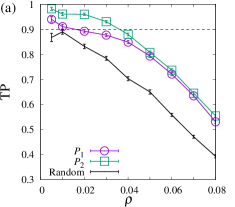
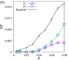
Fig.1 shows the-$\rho$-dependence of (a) TP and (b) FP at $N=1000$, $M=400$ with $M_{\mathrm{ini}}=300$ and $M_{\mathrm{ada}}=100$. The error probabilities are set at $p_{\mathrm{TP}}=0.9$ and $p_{\mathrm{FP}}=0.05$, and the group size in the initial stage is $N_{G}=10$. $P_{1}$ and $P_{2}$ in the figure denote the results of the active pooling in the spaces ${\cal P}_{1}$ and ${\cal P}_{2}$, respectively . For comparison, the results of random pooling are shown, where tests in $M_{\mathrm{ada}}$ steps are performed on random pools generated by the same rule as the initial $M_{\mathrm{ini}}$-times tests. Each data point represents the averaged value with respect to 100 realizations of $\bm{Y}_{(M_{\mathrm{ini}})}$, $\bm{F}_{(M_{\mathrm{ini}})}$ and $\bm{X}^{(0)}$. For any region of $\rho$, TP under a random test cannot exceed the $p_{\mathrm{TP}}$, which is indicated by the horizontal line in Fig.1 (a). The adaptive test improves TP and achieves $\mathrm{TP}>p_{\mathrm{TP}}$ when $\rho<0.02$ for ${\cal P}_{1}$ case and $\rho<0.04$ for ${\cal P}_{2}$ case. As shown in Fig.1 (b), FP is smaller than $p_{\mathrm{FP}}$ even when the pooling is randomly determined, but the adaptive test can further decrease FP.

Figure 2: $M$-dependence of (a) true-positive and (b) false-positive at $N=1000$ and $\rho=0.02$. The adaptive tests are performed $100$ times after $M_{\mathrm{ini}}=300,~{}400$, and 500 random tests with $N_{G}=10$. The error probabilities on the test are fixed at $p_{\mathrm{TP}}=0.9$ and $p_{\mathrm{FP}}=0.05$. The horizontal dashed line in (a) represents $p_{\mathrm{TP}}$.

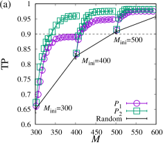
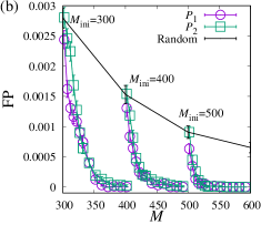
The performance of the adaptive test depends on the number of initial random tests $M_{\mathrm{ini}}$. Fig.2 shows the $M_{\mathrm{ini}}$-dependence of (a) TP and (b) FP at $N=1000$, $\rho=0.02$, $p_{\mathrm{FP}}=0.9$, and $p_{\mathrm{TP}}=0.05$. The pool size at the initial stage is $N_{G}=10$. The figure also presents the results for $M_{\mathrm{ini}}=300$, 400, and 500. The horizontal dashed line in (a) represents the TP probability of the test, which is 0.9. As $M_{\mathrm{ini}}$ increases, a high TP close to 1 is obtained via the adaptive test. Moreover, for a large $M_{\mathrm{ini}}$, such as $M_{\mathrm{ini}}=500$, the possible pooling space does not significantly influence the performance in terms of TP and FP. Meanwhile, for a small $M_{\mathrm{ini}}$, the result of TP depends on the pooling space, and more accurate identification is achieved by ${\cal P}_{2}$. The test results at the initial stage have large uncertainties when $M_{\mathrm{ini}}$ is small, and hence, it is considered that the large pooling space is required for the effective sampling of the uncertain pools.

As shown in Fig.2 (a), to achieve a high TP, the active pooling method requires a smaller number of tests than that required by the random pooling method. For instance, the active pooling in ${\cal P}_{2}$ with $M_{\mathrm{ini}}=300$ initial stage results in a high $\mathrm{TP}>p_{\mathrm{TP}}$ after the $M_{\mathrm{ada}}=40$ adaptive stage, namely $M=340$. Meanwhile, the random pooling achieves $\mathrm{TP}>p_{\mathrm{TP}}$ with almost $M=500$ tests. With regard to the improvement of TP, the adaptive method helps effectively identify infected patients with a small number of tests.

Figure 3: $p_{\mathrm{TP}}$-dependence of true-positive for (a) $p_{\mathrm{FP}}=0.05$ and (b) $p_{\mathrm{TP}}=0.95$ at $N=1000$ and $\rho=0.02$. The adaptive tests are conducted $100$ times after $M_{\mathrm{ini}}=300$; hence, $M=400$ in total. The pool size in the random tests is $N_{G}=10$. The horizontal dashed lines represent $\mathrm{TP}=p_{\mathrm{TP}}$.

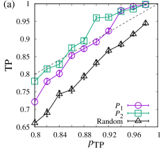
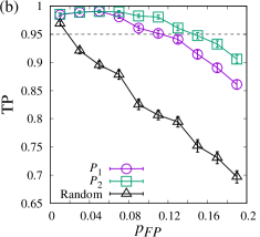
The active pooling is robust to the errors in the test, compared with the random pooling. Fig.3 shows (a) the $p_{\mathrm{TP}}$-dependence of TP for $p_{\mathrm{FP}}=0.05$ and (b) the $p_{\mathrm{FP}}$-dependence of TP for $p_{\mathrm{TP}}=0.95$ at $N=1000$, $M_{\mathrm{ini}}=300$, $M_{\mathrm{ada}}=100$, and $\rho=0.02$. The random tests in the initial stage are performed on pools of size $N_{G}=10$. For the random pooling case, $\mathrm{TP}>p_{\mathrm{TP}}$ is achieved only when $p_{\mathrm{FP}}$ is sufficiently small such as $p_{\mathrm{FP}}<0.02$. The adaptive test improves TP, and the parameter region where $\mathrm{TP}>p_{\mathrm{TP}}$ is extended in particular for the case ${\cal P}_{2}$.

These results indicate the efficiency of the active pooling design based on predictive distribution in group testing. However, a limitation of this approach is that the computational cost involved is higher than that of the non-adaptive approach. The estimation of the infection probability via the BP algorithm $M_{\mathrm{ada}}$ steps is obtained again; hence, the computational cost of the adaptive approach is approximately $M_{\mathrm{ada}}$ times larger than that of the non-adaptive approach. However, the adaptive approach achieves accurate estimation using a small number of tests. The trade-off between the reduction of the operating cost involved in tests and the increase in the computation time of inference should be considered for practically apply the adaptive approach.

V Summary and discussion

In this paper, we propose an active pooling design in adaptive group testing, where the pool for the subsequent stage is determined based on the Bayesian posterior predictive distribution under the test outcomes in the previous stage. The proposed method was implemented using the BP algorithm, and the identification of infected patients using adaptive tests is demonstrated to be more accurate than that using randomly designed pools. In particular, the active pooling design reduced the number of required tests to achieve $\mathrm{TP}>p_{\mathrm{TP}}$. Further, the proposed method is robust to test errors and $\mathrm{TP}>p_{\mathrm{TP}}$ holds in smaller $p_{\mathrm{TP}}$ and larger $p_{\mathrm{FP}}$, compared with the approach that uses randomly designed pools.

In the current study, we restrict the possible pooling space within ${\cal P}_{1}$ and ${\cal P}_{2}$. Mathematically, more uncertain pool can be considered removing this restriction, and further improvement in the TP and FP rates is expected. However, the straightforward calculation of the predictive entropy for all possible $\pi$ is computationally intractable. Hence, some approximation will be required. An efficient sampling method in $\pi\in{\cal P}$ to find the uncertain pool should be developed such as the Markov chain Monte Carlo method.

We focused on the MAP estimator to convert the estimated infection probability, which is $[0,1]$ variable, into the state of patients, $\{0,1\}$ variable, because of its simplicity; however, changing the decision threshold from 0.5 results in improvements in the TP rate. For example, the estimate using the confidence interval constructed based on the bootstrap method was obtained. Further, the TP rate obtained using this method is higher than that obtained using the MAP estimator [20]; however, its computational cost is unrealistic to accompany the active pooling procedure. The receiver operating characteristic (ROC) analysis is a promising method to understand the appropriate decision threshold [25, 26]. Along with the ROC analysis, the mathematical background of the active pooling proposed in this paper is expected to be established.

Appendix A BP algorithm for group testing

We denote $\pi(\mu)$ and ${\cal G}(i)$ as the indices of the patients in the $\mu$-th pool and those of the pools in which the $i$-th patient is included, respectively. For the edge that connects the $\mu$-th factor (test) and the $i$-th variable (patient), two types of messages $m_{i\to\mu}(X_{i})$ and $\tilde{m}_{\mu\to i}(X_{i})$ are defined. Intuitively, the messages $m_{i\to\mu}(X_{i})$ and $\tilde{m}_{\mu\to i}(X_{i})$ represent the marginal distributions of $X_{i}$ before and after the $\mu$-th test is performed, respectively. The variable $X_{i}$ is binary. Hence, the messages can be expressed by the Bernoulli probability $\theta_{i\to\mu}$ and $\tilde{\theta}_{\mu\to i}$ given by

$$\theta_{i\to\mu}=\frac{\rho\prod_{\nu\in{\cal G}(i)\backslash\mu}\tilde{\theta}_{\nu\to i}}{Z_{i\to\mu}},~{}~{}~{}\tilde{\theta}_{\mu\to i}=\frac{U_{\mu}}{\tilde{Z}_{\mu\to i}}$$ (14)

where $U_{\mu}=p_{\mathrm{TP}}Y_{\mu}+(1-p_{\mathrm{TP}})(1-Y_{\mu})$, $W_{\mu}=p_{\mathrm{FP}}Y_{\mu}+(1-p_{\mathrm{FP}})(1-Y_{\mu})$ and

$$\tilde{Z}_{\mu\to i} =U_{\mu}\left(2-\prod_{j\in\pi(\mu)\backslash i}(1-\theta_{j\to\mu})\right)+W_{\mu}\prod_{j\in\pi(\mu)\backslash i}(1-\theta_{j\to\mu})$$ (15)

$$Z_{i\to\mu} =\rho\prod_{\nu\in{\cal G}(i)\backslash\mu}\tilde{\theta}_{\nu\to i}+(1-\rho)\prod_{\nu\in{\cal G}(i)\backslash\mu}(1-\tilde{\theta}_{\nu\to i}).$$ (16)

The BP algorithm consists of the recursive update of $\theta_{i\to\mu}$ and $\tilde{\theta}_{\mu\to i}$, and at the fixed point, the infection probability is given by [18, 17, 20]

$$\hat{\theta}_{i}=\frac{\rho\prod_{\mu\in{\cal G}(i)}\tilde{\theta}_{\mu\to i}}{\rho\prod_{\mu\in{\cal G}(i)}\tilde{\theta}_{\mu\to i}+(1-\rho)\prod_{\mu\in{\cal G}(i)}(1-\tilde{\theta}_{\mu\to i})}.$$ (17)

Appendix B Calculation of susceptibility using the BP algorithm

Figure 4: (a) Examples of susceptibility calculated using the BP algorithm and exact computation at $N=20$, $M=10$, $N_{G}=10$, $N_{O}=5,\rho=0.1$, $p_{\mathrm{TP}}=0.95$, and $p_{\mathrm{FP}}=0.05$. $\chi_{ij}$ for $j=20$ is shown for two different realizations of $\bm{Y},\bm{F}$, and $\bm{X}^{(0)}$. (b) Quantification of the difference between susceptibilities given by the BP algorithm and the exact calculations at $N=20$ and $N_{G}=10$ for several parameters using $\epsilon$.

Figure 5: Comparison of (a) true-positive and (b) false-positive for ${\cal P}_{2}$ case considering the susceptibility, ${\cal P}_{2}$ case without considering the susceptibility, and ${\cal P}_{1}$ case, at $N=200$, $M_{\mathrm{ini}}=80$, $\rho=0.05$, $p_{\mathrm{TP}}=0.9$, and $p_{\mathrm{FP}}=0.1$. The tests in the initial stage are performed on the randomly designed pools with $N_{G}=10$ and $N_{O}=4$.

A widely used method to calculate susceptibility in the framework of the BP algorithm is susceptibility propagation [27, 28], where recursive update of tensors that give susceptibility is introduced on the basis of linear-response theory. In the current problem setting, the variables to be estimated obey the Bernoulli probability. Hence, we can compute the susceptibility in a simpler way.

Let us denote the expectation of $X_{j}$ under the posterior conditional distribution $\sum_{\bm{X}\backslash i,j}P_{\mathrm{post}}(X_{j},X_{i}=1,\bm{X}_{\backslash i,j}|\bm{Y})$ as $\theta_{j}^{|X_{i}=1}\equiv E_{\mathrm{post}|\bm{Y}}[X_{j}|X_{i}=1]$ $(i\neq j)$. This expectation value is evaluated using the BP algorithm by fixing $\theta_{i\to\mu}=1$ and $\tilde{\theta}_{\mu\to i}=1$ for $\mu\in{\cal G}(i)$. The conditional expectation value obtained using the BP algorithm is denoted as $\hat{\theta}_{j}^{|X_{i}=1}$. Thus, the susceptibility is given by $\hat{\chi}_{ij}=\hat{\theta}_{i}\hat{\theta}_{j}^{|X_{i}=1}-\hat{\theta}_{i}\hat{\theta}_{j}$. We can show that the symmetry $\hat{\theta}_{i}\hat{\theta}_{j}^{|X_{i}=1}=\hat{\theta}_{i}^{|X_{j}=1}\hat{\theta}_{j}$ holds.

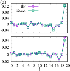
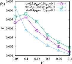
To check the accuracy of the susceptibility derived using the BP algorithm, we compute the exact posterior distribution by sampling all configurations in $\{0,1\}^{N}$. Examples of the exact susceptibility and the approximated one are shown in Fig.4(a) at $N=20$, $M=10$, $\rho=0.1$, $p_{\mathrm{TP}}=0.95$, and $p_{\mathrm{FP}}=0.05$, where the $i$-dependence of $\chi_{i,20}$ is shown for two different realizations of $\bm{Y},\bm{F}$, and $\bm{X}^{(0)}$. Here, the pooling matrix is randomly generated to be $N_{G}=10$ and $N_{O}=5$. The difference between $\chi$ and $\hat{\chi}$ is quantified by $\epsilon\equiv\sum_{i<j}(\chi_{ij}-\hat{\chi}_{ij})^{2}/\{N(N-1)/2\}$, whose behavior is shown in Fig.4 (b) at $N=20$ and different values of $\alpha\equiv M/N$, $p_{\mathrm{TP}}$, and $p_{\mathrm{FP}}$. For any parameter region, $\epsilon$ is $O(10^{-3})$. Therefore, we consider that the BP algorithm provides a reasonable approximation of the susceptibility and expect that it is also applicable for larger $N$.

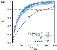
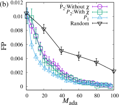
In Fig.5, (a) TP and (b) FP are shown for the cases when the susceptibility is considered (denoted by ‘$P_{2}$: with $\chi$’) and not considered (denoted by ‘$P_{2}$: without $\chi$’); namely, eq.(12) is used to determine the pool in the subsequent stage by substituting $\hat{\chi}$ calculated by BP into $\chi$ at $N=200$, $\rho=0.05$, $p_{\mathrm{TP}}=0.9$, and $p_{\mathrm{FP}}=0.1$. Each data point is averaged over 50 samples of $\bm{F}$, $\bm{X}^{(0)}$, and $\bm{Y}$. The initial stage consists of $M_{\mathrm{ini}}=80$ random tests with $N_{G}=10$ and $N_{O}=4$. The ${\cal P}_{1}$ case is compared with the random case with the same test at the initial stage. Considering the susceptibility, a slight improvement in TP is observed.

Following the same procedure, we can compute a higher order correlation in principle. For example, $E_{\mathrm{post}|\bm{Y}}[X_{i}|X_{j}=1,X_{k}=1]$ is obtained by fixing $\theta_{j\to\mu}=1$, $\theta_{k\to\nu}=1$, and $\tilde{\theta}_{\mu\to j}=1$, $\tilde{\theta}_{\nu\to k}=1$ for $\mu\in{\cal G}(j)$ and $\nu\in{\cal G}(k)$.

References

- Dorfman [1943] R. Dorfman, Ann.Math.Statist. 14, 436 (1943).
- Du and K. Hwang [2000] D.-Z. Du and F. K. Hwang, Combinatorial Group Testing and Its Applications (World Scientific, 2000).
- Sobel and A. Groll [1959] M. Sobel and P. A. Groll, Bell System tech. J. 28, 1179 (1959).
- Wolf [1985] J. K. Wolf, IEEE Transactions on Information Theory 31, 185 (1985).
- Sobel and Groll [1959] M. Sobel and P. A. Groll, Bell Labs Technical Journal 38, 1179 (1959).
- Sobel and Groll [1966] M. Sobel and P. A. Groll, Technometrics 8, 631 (1966).
- K. Hwang [1972] F. K. Hwang, Journal of the American Statistical Association 67, 605 (1972).
- V. Fedorov [1972] V. V. Fedorov, Theory of Optimal Experiments (Academic Press (New York), 1972).
- Pukelsheim [1972] F. Pukelsheim, Optimal Design of Experiments (Academic Press (New York), 1972).
- A. Cohn et al. [1996] D. A. Cohn, Z. Ghahramani, and M. I. Jordan, Journal of Artificial Intelligence Research 4, 129 (1996).
- Settles [2009] B. Settles, Active learning literature survey, Tech. Rep. (University of Wisconsin-Madison Department of Computer Sciences, 2009).
- Brochu et al. [2010] E. Brochu, V. M. Cora, and N. de Freitas, A tutorial on bayesian optimization of expensive cost functions, with application to active user modeling and hierarchical reinforcement learning, https://arxiv.org/abs/1012.2599 (2010).
- Shahriari et al. [2015] B. Shahriari, K. Swersky, Z. Wang, P. A. R, and N. De Freitas, Proceedings of the IEEE 104, 148 (2015).
- Zhu et al. [2003] X. Zhu, J. Lafferty, and Z. Ghahramani, in ICML-2003 Workshop on The Continuum from Labeled to Unlabeled Data (2003) pp. 58–65.
- Tong and Koller [2001] S. Tong and D. Koller, Journal of Machine Learning Research 2, 45 (2001).
- Mézard and Montanari [2009] M. Mézard and A. Montanari, Information, physics, and computation (Oxford University Press, 2009).
- Mézard et al. [2008] M. Mézard, M. Tarzia, and C. Toninelli, Journal of Physics: Conference Series 95, 012019 (2008).
- Sejdinovic and Johnson [2010] D. Sejdinovic and O. Johnson, in 48th Annual Allerton Conference on Communication, Control, and Computing (Allerton) (IEEE, 2010) pp. 998 – 1003.
- Kanamori et al. [2012] T. Kanamori, H. Uehara, and M. Jimbo, Journal of Statistical Theory and Practice 6, 220 (2012).
- Sakata [2020] A. Sakata, Journal of Physical Society of Japan 89, 084001 (2020).
- Kitagawa [1997] G. Kitagawa, Communications in statistics - theory and methods 26, 2223 (1997).
- D. Lewis and A. Gale [1994] D. D. Lewis and W. A. Gale, in ACM SIGIR Conference on Research and Development in Information Retrieval (ACM/Springer, 1994) pp. 3–12.
- D. Lewis and Catlett [1994] D. D. Lewis and J. Catlett, in International Conference on Machine Learning (ICML) (Morgan Kaufmann, 1994) pp. 148–156.
- Note [1] We note the heuristics used in the simulation. When is sufficiently small such as , BP for the active pooling does not converge sometimes. This is due to the overlapped pools; that is, certain pools are selected several times in the adaptive stage. It is known that rank deficiency can cause the instability of BP. To avoid this problem, we exclude the already existing pool from the candidates in the subsequent stage for the small- case.
- Kumar and Indrayan [2011] R. Kumar and A. Indrayan, Indian Pediatr 48, 277 (2011).
- Hajian-Tilaki [2013] K. Hajian-Tilaki, Caspian J Intern Med 4, 627 (2013).
- Mézard and Mora [2009] M. Mézard and T. Mora, J Physiol Paris 103, 107 (2009).
- Yasuda and Tanaka [2013] M. Yasuda and K. Tanaka, Physical Review E 87, 012134 (2013).