Conservative semi-Lagrangian schemes for kinetic equations
Part I: Reconstruction

Abstract.

In this paper, we propose and analyse a reconstruction technique which enables one to design high-order conservative semi-Lagrangian schemes for kinetic equations. The proposed reconstruction can be obtained by taking the sliding average of a given polynomial reconstruction of the numerical solution. A compact representation of the high order conservative reconstruction in one and two space dimension is provided, and its mathematical properties are analyzed. To demonstrate the performance of proposed technique, we consider implicit semi-Lagrangian schemes for kinetic-like equations such as the Xin-Jin model and the Broadwell model, and then solve related shock problems which arise in the relaxation limit. Applications to BGK and Vlasov-Poisson equations will be presented in the second part of the paper.

1. Introduction

Kinetic equations and quasi-linear systems of conservation laws are strongly related. For example, the behavior of rarefied gas is well described by the Boltzmann transport equation (BTE) [10]. Once velocity space is discretized, BTE has the mathematical structure of a semi-linear hyperbolic system of balance laws. In the so-called fluid dynamic limit, the distribution function approaches the Maxwellian whose parameters satisfy the Euler equations of gas dynamics, which is a quasi-linear system of conservation laws. The Broadwell model of the BTE in one space dimension is a semi-linear $3\times 3$ relaxation system. As the relaxation parameter vanishes, the model relaxes to a $2\times 2$ quasi-linear hyperbolic system of conservation laws. An implicit treatment of the collision term using L-stable schemes allows the construction of asymptotic preserving schemes which become consistent schemes of the relaxed limit [4, 31, 22].

Quasi-linear hyperbolic systems generically develop jump discontinuities in finite time. Most schemes for their numerical solutions are based on two fundamental ingredients: conservation and non-oscillatory reconstruction. Finite volume and finite difference methods have been widely used for the discretization of the convective terms of kinetic models (Eulerian approach), which are usually treated explicitly. In this way, it is relatively easy to construct conservative schemes. Conservation is relevant especially in the relaxed limit: lack of conservation will prevent weak consistency of the method for discontinuous solutions leading, for example, to $\mathcal{O}(1)$ errors in the propagation of shocks.

Conservative non-oscillatory reconstruction such as the ENO or WENO methology [35] have been widely adopted in many practical problems [7, 9, 30]. The approach has been extended to a compact WENO (CWENO [6, 12, 13, 27, 28, 29]) reconstruction which gives uniform accuracy in a whole cell, and it allows the construction of efficient high order finite volume scheme in several space dimensions [16]. Unfortunately, explicit Eulerian schemes cannot avoid CFL-type time step restrictions imposed by converction-like terms in hyperbolic equations.

To treat this difficulty, semi-Lagrangian approaches recently have gained popularity because they do not suffer from such CFL-type time step restriction which arises in the treatment of Eulerian counterparts. Instead, since the semi-Lagrangian method is obtained by integrating the equations along its characteristics, this approach necessarily requires the computation of numerical solutions on off-grid points by a reconstruction which makes use of the numerical solutions on grid points.

If one uses piecewise Lagrange polynomial reconstruction, then conservation is guaranteed if the same stencil is used in each cell, because of translation invariance (we shall call this a linear reconstruction). On the other hand, such linear reconstruction may introduce spurious oscillations of may cause loss of positivity. If one wants to prevent appearing of spurious oscillations, then one can use high-order non-oscillatory reconstruction, such as ENO of WENO [35, 7, 8]. Similarly, positivity of the numerical solution can be maintained by positivity-preserving reconstructions [5, 34]. Unfortunately these non-linear reconstructions destroy the translation invariance guaranteed by linear reconstruction, causing lack of conservation [1].

Numerous approaches have been introduced to treat such difficulties, and maintain conservation even with non-linear reconstruction. In particular, in the context of Vlasov-Poisson system several techniques were proposed. Among them, we mention the work based on primitive polynomial reconstruction [18, 14, 32]. In [18], the authors developed the Positive and Flux Conservative scheme. The authors considered essentially non-oscillatory method (ENO) or reconstructions based on positive limiters. In [14], the authors took a similar approach in the construction of primitive functions using splines. An weighted essentially non-oscillatory method (WENO) is also proposed to construct high order conservative non-oscillatory schemes in [32]. All these method are either one-dimensional or they provide a dimension by dimension interpolation. A general technique to restore conservation in semi-Lagrangian schemes was presented in [33]. The technique has been also applied to the BGK model [1]. Although quite general, the technique suffers from CFL-type stability restrictions.

In this paper we present a general technique which allows the construction of high-order conservative non-oscillatory semi-Lagrangian schemes in one and several dimensions, which are not affected by CFL-type restriction. Given cell averaged values on uniform grids, the idea is to compute sliding average of a precomputed non-oscillatory piecewise polynomial reconstruction.

The resulting reconstruction inherits the non-oscillatory properties of the precomputed polynomial and guarantees conservation of all discrete moments. The technique requires characteristic lines are parallel, which is the case of kinetic equations in which velocity space is discretized on the same velocity grid throughout space. An advantage of our method is that one can easily adopt previous techniques such as ENO, WENO, CWENO polynomials as our basic reconstructions.

The mathematical properties of the proposed reconstruction are analyzed. In particular, we show that if we take CWENO polynomials of even degree $k$, for example $k=2,4$ [6, 28], as a basic reconstruction, our approach gives $k+2$th order accuracy. Similar properties are also generalized to two dimensional reconstruction with CWENO polynomial in two space dimensions [28]. The description of technique is provided in the sense of cell averages, however, the idea can be extended to the point-wise framework in a similar manner.

To test the quality of the proposed reconstruction, we apply it to the finite difference implicit semi-Lagrangian schemes for semi-linear hyperbolic system such as Xin-Jin model or Broadwell model. Applications to more general equations will be presented in a companion paper.

This paper is organized as follows: In section 2, we present a general framework for our conservative reconstruction in 1D and its related properties. section 3 is devoted to the conserative reconstruction in 2D. Semi-Lagrangian methods are described in section 4. In section 5, several numerical tests are presented to verify the accuracy of the proposed schemes and its capability in treating shocks arising in the relaxation of semi-linear hyperbolic system.

2. Conservative reconstruction in 1D

Let $u:\mathbb{R}\rightarrow\mathbb{R}$ be a smooth function and $\bar{u}:\mathbb{R}\rightarrow\mathbb{R}$ be a corresponding sliding average function:

$$\frac{1}{\Delta x}\int_{x-\Delta x/2}^{x+\Delta x/2}u(y)\,dy=\bar{u}(x).$$

Given cell averages on uniform grids $x_{i}=i\Delta x$:

$$\frac{1}{\Delta x}\int_{I_{i}}u(x)\,dx=\bar{u}_{i},\quad I_{i}=[x_{i-\frac{1}{2}},x_{i+\frac{1}{2}}],$$

for each $i\in\mathcal{I}$, our goal is to construct an approximation $Q(x)$ of the sliding average $\bar{u}(x)$, which is conservative in the sense that for any periodic function $\bar{u}(x)$ with period $L=N\Delta x$, $N\in\mathbb{N}$, we have

$$\sum_{i=1}^{N}Q(x_{i}+\theta)=\sum_{i=1}^{N}\bar{u}(x_{i}),\quad\theta\in[0,1).$$

Assume we have a piecewise smooth reconstruction $R(x)=\sum_{i}R_{i}(x)\chi_{i}(x)$, for $i\in\mathcal{I}$, where $\chi_{i}(x)$ denotes the characteristic function of cell $i$ and each $R_{i}(x)$ denotes a polynomial of degree $k$ and has the following properties:

1. High order accuracy in the approximation of $u(x)$:

   (2.1) $$u(x)=R_{i}(x)+\mathcal{O}\left((\Delta x)^{k+1}\right),\quad x\in I_{i}.$$

2. Conservation in the sense of cell averages:

   $$\frac{1}{\Delta x}\int_{x_{i-\frac{1}{2}}}^{x_{i+\frac{1}{2}}}R_{i}(x)\,dx=\bar{u}_{i}.$$

Consider a shifted interval $[y_{i-\frac{1}{2}},y_{i+\frac{1}{2}}]$ whose center is $x_{i+\theta}\equiv x_{i}+\theta\Delta x$, $\theta\in[0,1)$, and denote by $\bar{u}(x_{i+\theta})$ the sliding average of $u$ at $x_{i+\theta}$ (see Fig. 1). We see that

$$x_{i-\frac{1}{2}}\leq y_{i-\frac{1}{2}}<x_{i+\frac{1}{2}}\leq y_{i+\frac{1}{2}}<x_{i+\frac{3}{2}}.$$

Our strategy is to approximate $\bar{u}(x_{i+\theta})$ by $Q_{i+\theta}\equiv Q(x_{i+\theta})$, where

(2.2) $$Q_{i+\theta}=\frac{1}{\Delta x}\int_{y_{i-\frac{1}{2}}}^{y_{i+\frac{1}{2}}}R(x)\,dx=\frac{1}{\Delta x}\int_{x_{i-\frac{1}{2}+\theta}}^{x_{i+\frac{1}{2}+\theta}}R(x)\,dx,$$

which is equivalent to

(2.3) $$Q_{i+\theta}=\frac{1}{\Delta x}\int_{x_{i-\frac{1}{2}+\theta}}^{x_{i+\frac{1}{2}}}R_{i}(x)\,dx+\frac{1}{\Delta x}\int_{x_{i+\frac{1}{2}}}^{x_{i+\frac{1}{2}+\theta}}R_{i+1}(x)\,dx.$$

From now on, we consider $R_{i}(x)$ to be piecewise polynomials of degree $k$ of the form:

(2.4) $$R_{i}(x)=\sum_{\ell=0}^{k}\frac{R_{i}^{(\ell)}}{\ell!}(x-x_{i})^{\ell}.$$

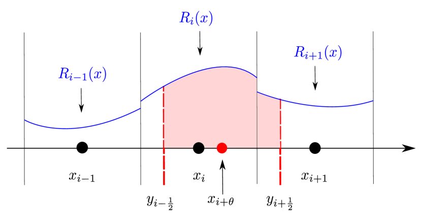
Figure 1. Description of one-dimensional conservative reconstruction

Making use of (2.4) in the first term, we obtain

$$\frac{1}{\Delta x}\int_{x_{i-\frac{1}{2}+\theta}}^{x_{i+\frac{1}{2}}}R_{i}(x)\,dx =\frac{1}{\Delta x}\sum_{\ell=0}^{k}R_{i}^{(\ell)}\int_{x_{i-\frac{1}{2}+\theta}}^{x_{i+\frac{1}{2}}}\frac{1}{\ell!}(x-x_{i})^{\ell}\,dx=\sum_{\ell=0}^{k}(\Delta x)^{\ell}R_{i}^{(\ell)}\alpha_{\ell}(\theta)$$

where

(2.5) $$\alpha_{\ell}(\theta)=\frac{1-(2\theta-1)^{\ell+1}}{2^{\ell+1}(\ell+1)!}.$$

Similarly, we can write

$$\frac{1}{\Delta x}\int_{x_{i+\frac{1}{2}}}^{x_{i+\frac{1}{2}+\theta}}R_{i+1}(x)\,dx :=\sum_{\ell=0}^{k}(\Delta x)^{\ell}R_{i+1}^{(\ell)}\beta_{\ell}(\theta),$$

with

(2.6) $$\beta_{\ell}(\theta)=\frac{(2\theta-1)^{\ell+1}-(-1)^{\ell+1}}{2^{\ell+1}(\ell+1)!}.$$

Letting $Q_{i+\theta}$ denote the approximation of $\bar{u}(x_{i+\theta})$, we obtain

(2.7) $$Q_{i+\theta}:=\sum_{\ell=0}^{k}(\Delta x)^{\ell}\left(\alpha_{\ell}(\theta)R_{i}^{(\ell)}+\beta_{\ell}(\theta)R_{i+1}^{(\ell)}\right).$$

Here, we note that $\alpha_{\ell}(\theta)$ and $\beta_{\ell}(\theta)$ satisfy the following relations:

• If $\ell=2n$, $0\leq n$, is a even number

  (2.8) $$\begin{split}\alpha_{\ell}(\theta)+\beta_{\ell}(\theta)=\frac{1}{(2n+1)!}\left(\frac{1}{2}\right)^{2n}.\end{split}$$

• If $\ell=2n+1$, $0\leq n$, is an odd number

  (2.9) $$\alpha_{\ell}(\theta)+\beta_{\ell}(\theta) =0.$$

We list the explicit form of $\alpha_{\ell}(\theta)$ and $\beta_{\ell}(\theta)$ for $\ell=0,1,2$:

(2.10) $$\begin{split}\alpha_{0}(\theta)&=1-\theta,\quad\alpha_{1}(\theta)=\frac{\theta(1-\theta)}{2},\quad\alpha_{2}(\theta)=\frac{1-q(\theta)}{24}\cr\beta_{0}(\theta)&=\theta,\quad\beta_{1}(\theta)=-\frac{\theta(1-\theta)}{2},\quad\beta_{2}(\theta)=\frac{q(\theta)}{24},\end{split}$$

where $q(\theta)=3\theta-6\theta^{2}+4\theta^{3}$, for $\theta\in[0,1)$.

2.1. General Properties

In this section, we provide several properties of the reconstruction (2.7) such as accuracy, conservation and consistency to the classical interpolation with a suitable choice of $R_{i}^{(\ell)}$ in the reconstruction.

Recalling the assumption (2.1), we have a function $R(x)$ which approximates point values of $u$ and our goal is to approximate sliding average function $\bar{u}$ with our reconstruction (2.7). Before checking the accuracy order, we note that the cell average function $\bar{u}(x)$ can be expressed in terms of derivatives of function $u(x)$:

(2.11) $$\begin{split}\bar{u}(x)&=\frac{1}{\Delta x}\int_{x-\Delta x/2}^{x+\Delta x/2}u(y)\,dy=\frac{1}{\Delta x}\int_{x-\Delta x/2}^{x+\Delta x/2}\sum_{\ell=0}^{\infty}\frac{u^{(\ell)}(x)}{\ell!}(y-x)^{\ell}\,dy=\sum_{\ell=\text{even}}^{\infty}\left(\Delta x\right)^{\ell}u^{(\ell)}(x)\frac{1}{(\ell+1)!}\left(\frac{1}{2}\right)^{\ell}.\end{split}$$

Inserting $x=x_{i+\theta}$ into (2.11), we obtain

$$\begin{split}\bar{u}(x_{i+\theta})&=\sum_{\ell=\text{even}}^{\infty}\left(\Delta x\right)^{\ell}u^{(\ell)}(x_{i+\theta})\frac{1}{(\ell+1)!}\left(\frac{1}{2}\right)^{\ell}=u^{(0)}(x_{i+\theta})+\frac{\left(\Delta x\right)^{2}}{24}u^{(2)}(x_{i+\theta})+\frac{\left(\Delta x\right)^{4}}{1920}u^{(4)}(x_{i+\theta})+\cdots.\end{split}$$

With this formula, in the following proposition, we provide a sufficient condition for a polynomial reconstruction $Q_{i+\theta}$ to be a $(k+2)$-th order accurate approximation of $\bar{u}(x+\theta)$ for $\theta\in[0,1)$.

Proposition 2.1.

Let $k\geq 0$ be an even integer, $R_{i}\in\mathbb{P}^{k}$ be given by (2.4), and $u$ be a smooth function $u:\mathbb{R}\in\mathbb{R}$. Suppose we have a piecewise polynomial $R(x)=\sum_{i}R_{i}(x)\chi_{i}(x)$, which satisfies

(2.12) $$\begin{split}u_{i}^{(\ell)}&=R_{i}^{(\ell)}+\mathcal{O}(\Delta x^{k+2-\ell}),\quad\text{$0\leq\ell\leq k$, whenever $\ell$ is an even integer}\cr u_{i}^{(\ell)}-u_{i+1}^{(\ell)}&=R_{i}^{(\ell)}-R_{i+1}^{(\ell)}+\mathcal{O}(\Delta x^{k+2-\ell}),\quad\text{$0\leq\ell<k$, whenever $\ell$ is an odd integer.}\end{split}$$

Then, the reconstruction $Q_{i+\theta}$ gives a $(k+2)$-th order approximation of the sliding average $\bar{u}(x_{i+\theta})$ for any $\theta\in[0,1)$.

Proof.

For detailed proof, see A. ∎

Remark 2.1.

1. The reconstruction $Q_{i+\theta}$ approximates $\bar{u}(x_{i+\theta})$ on the basis of cell average values $\{\bar{u}_{i}\}_{i\in\mathcal{I}}$. Similarly, we can extend the idea of reconstruction to the framework of point values, which are used in conservative finite difference methods in section 4.

2. We also note that the second condition in (2.12) can be easily satisfied. Let $k\geq 0$ be an even integer, and consider a function $u(x)\in C^{k+2}(\mathbb{R})$, and its primitive function $U(x):=\int_{-\infty}^{x}u(y)\,dy\in C^{k+3}(\mathbb{R})$. We first look for a polynomial $P_{i}(x)\in\mathbb{P}^{k+1}$ such that

   $$P_{i}(x_{i-\frac{1}{2}+j})=U(x_{i-\frac{1}{2}+j}),\quad j=-r,\cdots,s+1,\quad r+s=k.$$

   Then, the classical interpolation theory gives

   $$U(x)-P_{i}(x)=\frac{1}{(k+2)!}U^{(k+2)}(\xi_{i})\prod_{j=-r}^{s+1}(x-x_{i-\frac{1}{2}+j}),\quad\xi_{i}\in(x_{i-\frac{1}{2}-r},x_{i+\frac{1}{2}+s}),$$

   its first order derivative $p_{i}(x)\equiv P_{i}^{\prime}(x)\in\mathbb{P}^{k}$ interpolates $u$ in the sense of cell-average:

   $$\frac{1}{\Delta x}\int_{x_{i+j}-\Delta x/2}^{x_{i+j}+\Delta x/2}p_{i}(y)\,dy=\bar{u}_{i+j},\quad j=-r,\cdots,s,$$

   and, for $0\leq\ell\leq k$, its $(\ell+1)$-th derivative $p_{i}^{(\ell)}(x)\equiv P_{i}^{(\ell+1)}(x)\in\mathbb{P}^{k-\ell}$ satisfies

   (2.13) $$u^{(\ell)}(x)-p_{i}^{(\ell)}(x)=U^{(\ell+1)}(x)-P_{i}^{(\ell+1)}(x)=\frac{1}{(k+2)!}U^{(k+2)}(\xi_{i})\frac{d^{\ell+1}}{dx^{\ell+1}}\left(\prod_{j=-r}^{s+1}(x-x_{i-\frac{1}{2}+j})\right).$$

   Similarly, we can find polynomials $p_{i+1}(x)\in\mathbb{P}^{k}$ and $P_{i+1}(x)\in\mathbb{P}^{k+1}$ such that

   $$u^{(\ell)}(x+\Delta x)-p_{i+1}^{(\ell)}(x+\Delta x) =U^{(\ell+1)}(x+\Delta x)-P_{i+1}^{(\ell+1)}(x+\Delta x)$$

   $$=\frac{1}{(k+2)!}U^{(k+2)}(\xi_{i+1})\frac{d^{\ell+1}}{dx^{\ell+1}}\left(\prod_{j=-r}^{s+1}(x+\Delta x-x_{i+1-\frac{1}{2}+j})\right),$$

   where $\xi_{i+1}\in(x_{i+\frac{1}{2}-r},x_{i+\frac{3}{2}+s})$. Then, the relation $U^{(k+2)}(\xi_{i})-U^{(k+2)}(\xi_{i+1})=\mathcal{O}\left(\Delta x\right)$, gives

   $$\left(u^{(\ell)}(x_{i})-p_{i}^{(\ell)}(x_{i})\right)-\left(u^{(\ell)}(x_{i+1})-p_{i+1}^{(\ell)}(x_{i+1})\right)$$

   $$\qquad=\frac{1}{(k+2)!}\left(U^{(k+2)}(\xi_{i})-U^{(k+2)}(\xi_{i+1})\right)\left\{\frac{d^{\ell}}{dx^{\ell}}\left(\prod_{j=-r}^{s+1}(x-x_{i-\frac{1}{2}+j})\right)\right\}_{x=x_{i}}=\mathcal{O}\left((\Delta x)^{k+2-\ell}\right).$$

3. If $R_{i}^{(\ell)}$ can be represented with a Lipschitz function $F_{\ell}$:

   $$R_{i}^{(\ell)}=F_{\ell}\left(\bar{u}_{i-r},\cdots,\bar{u}_{i+s}\right)$$

   which satisfies

   $$F_{\ell}\left(\bar{u}_{i-r},\cdots,\bar{u}_{i+s}\right)-u^{(\ell)}(x_{i}) =\mathcal{O}\left((\Delta x)^{k+1-\ell}\right),$$

   the condition (2.12) is also satisfied. For more details, we refer to B.

In Proposition 2.1, we see that the choice of an even integer $k\geq 0$ leads to the improvement of accuracy. In such a case, we show that the reconstruction $Q_{i+\theta}$ based on linear weights coincides with the classical interpolation.

Proposition 2.2.

Let $k\geq 0$ be an even integer with $k=2r$. For each $i\in\mathcal{I}$, assume that we have a basic reconstruction $R_{i}(x)\in\mathbb{P}^{k}$, which is a polynomial of degree $k$ in (2.4) and interpolates the function $u$ in the sense of cell averages:

(2.14) $$\begin{split}\frac{1}{\Delta x}\int_{x_{i+j-\frac{1}{2}}}^{x_{i+j+\frac{1}{2}}}R_{i}(x)\,dx=\bar{u}_{i+j},\quad-r\leq j\leq r.\end{split}$$

with a symmetric stencil $S_{i}:=\{i-r,i-r+1,\cdots,i+r\}$. Then, the reconstruction $Q_{i+\theta}$ in (2.7) based on $R_{i}$ and $R_{i+1}$, is the Lagrange polynomial $L(x)$ that interpolates $\bar{u}_{i+j}$, for $-r\leq j\leq r+1$, where $x=x_{i}+\theta\Delta x$ and $\theta\in[0,1)$.

The proof is based on the observation that interpolation in the sense of the cell averages is equivalent to point-wise interpolation of sliding averages at cell center, which in turn, is equivalent to point-wise interpolation of primitive function at cell edges. A detailed proof, based on explicit representation obtained by Lagrange interpolation, is given in C.

Remark 2.2.

For $k=0$, the only possible choice is to set $R_{i}(x)\equiv\bar{u}_{i}$ and the resulting reconstruction $Q_{i+\theta}$ reduces to the linear interpolation constructed from two points $\bar{u}_{i}$ and $\bar{u}_{i+1}$.

In the following proposition, we show that total mass is preserved for any $\theta$-shifted summation, $\theta\in[0,1)$.

Proposition 2.3.

Assume that $R_{i}(x)$ satisfies

(2.15) $$\begin{split}\frac{1}{\Delta x}\int_{x_{i-\frac{1}{2}}}^{x_{i+\frac{1}{2}}}R_{i}(x)\,dx=\bar{u}_{i},\quad i\in\mathcal{I}.\end{split}$$

Then, for periodic functions $\bar{u}(x)$ with period $L=N\Delta x,\,N\in\mathbb{N}$

(2.16) $$\sum_{i=1}^{N}Q_{i+\theta}=\sum_{i=1}^{N}\bar{u}_{i},$$

for any $\theta\in[0,1)$.

Proof.

Since $\theta$ does not depend on $i$,

$$\sum_{i=1}^{N}Q_{i+\theta} =\sum_{i=1}^{N}\left(\frac{1}{\Delta x}\int_{x_{i-\frac{1}{2}+\theta}}^{x_{i+\frac{1}{2}}}R_{i}(x)\,dx+\frac{1}{\Delta x}\int_{x_{i+\frac{1}{2}}}^{x_{i+\frac{1}{2}+\theta}}R_{i+1}(x)\,dx\right)$$

$$=\sum_{i=1}^{N}\left(\frac{1}{\Delta x}\int_{x_{i-\frac{1}{2}+\theta}}^{x_{i+\frac{1}{2}}}R_{i}(x)\,dx+\frac{1}{\Delta x}\int_{x_{i-\frac{1}{2}}}^{x_{i-\frac{1}{2}+\theta}}R_{i}(x)\,dx\right)$$

$$=\sum_{i=1}^{N}\frac{1}{\Delta x}\int_{x_{i-\frac{1}{2}}}^{x_{i+\frac{1}{2}}}R_{i}(x)\,dx=\sum_{i=1}^{N}\bar{u}_{i}.$$

Here we used the periodicity to write the second line and (2.15) for the last line. ∎

Remark 2.3.

We remark that this summation preserving property can be useful when our reconstruction is applied to the semi-Lagrangian treatment of a constant convection term, where characteristic curves are given by parallel lines for each grid point. In such cases, the proposed reconstruction attains conservation at a discrete level, hence it can be applied to the simulation of physical models satisfying this conservation property. Considerable examples are the BGK type models of the Boltzmann equation of rarefied gas dynamics. We can also apply this to the splitting method for the Vlasov-Poisson system in plasma physics. These problems will be considered in the second part of this paper.

In the following section, we will show that our reconstruction (2.7) inherits some properties of the basic reconstruction $R_{i}(x)$ such as non-oscillatory property and positivity.

2.2. Choice of the basic reconstruction $R$

2.2.1. Non-oscillatory property

We consider some specific choices of the basic reconstruction $R$. In particular, we consider CWENO [6], [28] and CWENOZ [13]. As an illustration, we consider the case $k=2$, and we take CWENO23 reconstruction in [28] as a basic reconstruction $R$. We start from a polynomial of degree two $P_{OPT}^{i}(x)$ which interpolates $\bar{u}_{i-1},\bar{u}_{i},\bar{u}_{i+1}$ in the sense of cell averages:

$$\frac{1}{\Delta x}\int_{x_{i+l-\frac{1}{2}}}^{x_{i+l+\frac{1}{2}}}P_{OPT}^{i}(x)\,dx=\bar{u}_{i+l},\quad l=-1,0,1.$$

Then, this polynomial can be written as $P_{OPT}^{i}(x)=\tilde{u}_{i}+\tilde{u}^{\prime}_{i}(x-x_{i})+\frac{1}{2}\tilde{u}^{\prime\prime}_{i}(x-x_{i})^{2}$ with

$$\tilde{u}_{i}=\bar{u}_{i}-\frac{1}{24}(\bar{u}_{i+1}-2\bar{u}_{i}+\bar{u}_{i-1}),\quad\tilde{u}^{\prime}_{i}=\frac{\bar{u}_{i+1}-\bar{u}_{i-1}}{2\Delta x},\quad\tilde{u}^{\prime\prime}_{i}=\frac{\bar{u}_{i+1}-2\bar{u}_{i}+\bar{u}_{i-1}}{({\Delta x})^{2}},$$

and it gives a third order accurate reconstruction of $u$ in $I_{i}$:

$$P_{OPT}^{i}(x)=u(x)+\mathcal{O}(\Delta x)^{3},\quad\forall x\in I_{i}.$$

In the CWENO23 reconstruction, to avoid oscillations, we use the following convex combination:

(2.17) $$R_{i}(x)=\sum_{k}\omega_{k}^{i}P_{k}^{i}(x),\quad\sum_{k}\omega_{k}^{i}=1,\quad\omega_{k}^{i}\geq 0,\quad k\in\{L,C,R\}$$

where $P_{L}^{i}$ and $P_{R}^{i}$ are first order polynomials such that

$$\int_{x_{i+l-\frac{1}{2}}}^{x_{i+l+\frac{1}{2}}}P_{L}^{i}(x)\,dx=\bar{u}_{i+l},\quad l=-1,0,\quad\quad\int_{x_{i+l-\frac{1}{2}}}^{x_{i+l+\frac{1}{2}}}P_{R}^{i}(x)\,dx=\bar{u}_{i+l},\quad l=0,1,$$

which gives

$$P_{L}^{i}(x)=\bar{u}_{i}+\frac{\bar{u}_{i}-\bar{u}_{i-1}}{\Delta x}(x-x_{i}),\quad P_{R}^{i}(x)=\bar{u}_{i}+\frac{\bar{u}_{i+1}-\bar{u}_{i}}{\Delta x}(x-x_{i}).$$

The second order polynomial $P_{C}(x)$ is obtained from

$$P_{OPT}^{i}(x)=C_{L}P_{L}^{i}(x)+C_{R}P_{R}^{i}(x)+C_{C}P_{C}^{i}(x),$$

with a choice of positive coefficients such that

$$C_{L},C_{R},C_{C}\geq 0,\quad C_{L}=C_{R},\quad C_{L}+C_{C}+C_{R}=1.$$

A common choice is to set $C_{L}=C_{R}=1/4$, $C_{C}=1/2$. The non-linear weights $\omega_{k}^{i}$ in (2.17) are chosen as follows:

(2.18) $$\omega_{k}^{i}=\frac{\alpha_{k}^{i}}{\sum_{\ell}\alpha_{\ell}^{i}},\quad\alpha_{k}^{i}=\frac{C_{i}}{(\epsilon+{\beta}_{k}^{i})^{p}},\quad k,\ell\in\{L,C,R\}$$

where the constant $\epsilon$ is used to avoid the denominator vanishing and the constant $p$ weights the smoothness indicator. We use $\epsilon=(\Delta x)^{2}$ or $10^{-6}$ and $p=2$ in the numerical tests. An explicit expression of smoothness indicators is the following:

$${\beta}_{L}^{i} =(\bar{u}_{i}-\bar{u}_{i-1})^{2},\quad{\beta}_{R}^{i}=(\bar{u}_{i+1}-\bar{u}_{i})^{2},$$

$${\beta}_{C}^{i} =\frac{13}{3}(\bar{u}_{i+1}-2\bar{u}_{i}+\bar{u}_{i-1})^{2}+\frac{1}{4}(\bar{u}_{i+1}-\bar{u}_{i-1})^{2}.$$

We refer to [27] for details on CWENO reconstruction. As a consequence, the reconstruction (2.17) is third order accurate in smooth region and automatically becomes second order accurate in the presence of discontinuity. The final form of the CWENO23 reconstruction $R_{i}(x)$ is given by

(2.19) $$R_{i}(x)=R_{i}^{(0)}+R_{i}^{(1)}(x-x_{i})+\frac{1}{2}R^{(2)}_{i}(x-x_{i})^{2},$$

where

$$R_{i}^{(0)}=\bar{u}_{i}-\frac{1}{12}\omega_{C}^{i}\left(\bar{u}_{i+1}-2\bar{u}_{i}+\bar{u}_{i-1}\right)$$

$$R_{i}^{(1)}=\omega_{L}^{i}\frac{\bar{u}_{i}-\bar{u}_{i-1}}{\Delta x}+\omega_{R}^{i}\frac{\bar{u}_{i+1}-\bar{u}_{i}}{\Delta x}+\omega_{C}^{i}\frac{\bar{u}_{i+1}-\bar{u}_{i-1}}{2\Delta x}$$

$$R_{i}^{(2)}=2\omega_{C}^{i}\frac{\bar{u}_{i+1}-2\bar{u}_{i}+\bar{u}_{i-1}}{(\Delta x)^{2}}.$$

The CWENO23Z reconstruction also takes the form (2.19), but its non-linear weights are calculated as follows:

(2.20) $$\omega_{k}^{i}=\frac{\alpha_{k}^{i}}{\sum_{\ell}\alpha_{\ell}^{i}},\quad\alpha_{k}^{i}=C_{i}\left(1+\frac{\tau}{\epsilon+{\beta}_{k}^{i}}\right)^{p},\quad k,\ell\in\{L,C,R\}$$

where $p\geq 1$ and $\tau=\left|\beta_{R}^{i}-\beta_{L}^{i}\right|$.

Remark 2.4.

In D, we prove that the condition (2.12) in Proposition 2.1 is satisfied both for CWENO23 and CWENO23Z if a given $u$ function is smooth enough. This shows that the corresponding reconstruction (2.19) becomes a fourth order accurate reconstruction for smooth solutions.

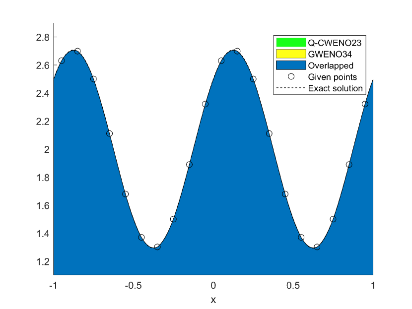
(a) Comparison of $\bar{u}_{1}$ is given by (2.21) and its reconstructions.

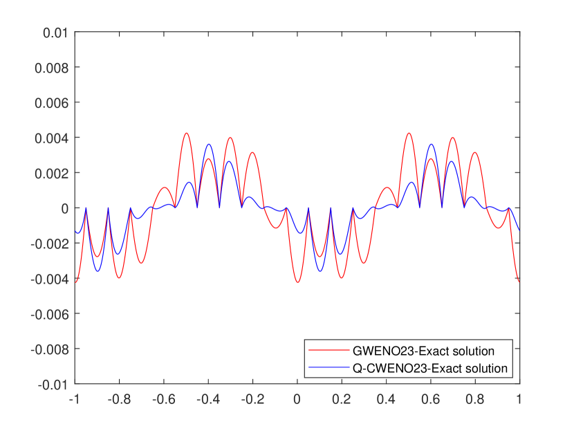
(b) Errors between reconstructions and exact solutions (2.21).

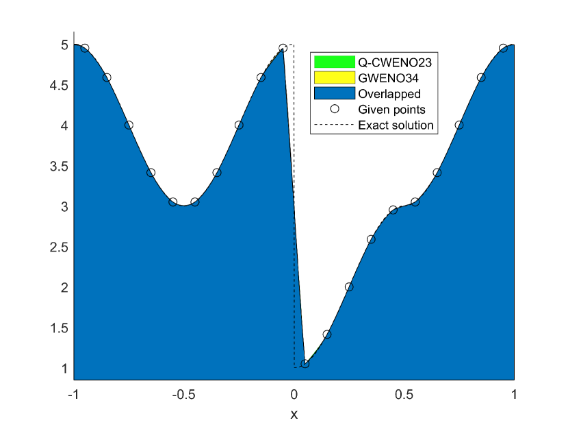
(c) Comparison of $\bar{u}_{2}$ is given by (2.22) and its reconstructions.

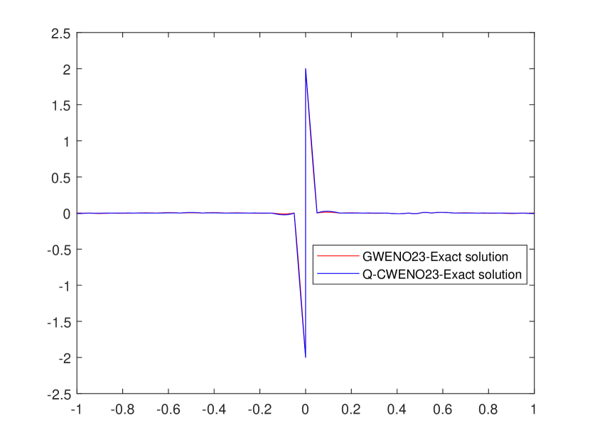
(d) Errors between reconstructions and exact solutions (2.22).

Figure 2. Comparison of reconstructions between Q-CWENO23 and GWENO34. In Figs.2(a) and 2(c), dashed lines are exact solutions $\bar{u}_{1}(x)$, $\bar{u}_{2}{x}$ and black circles are given values on grid points of $\bar{u}_{1}{x}$, $\bar{u}_{2}{x}$ in (2.21) and (2.22).

In Fig. 2, we compare the proposed conservative reconstruction (2.19) using CWENO23 [29] with a generalized WENO reconstruction originally proposed in [7] in the context of semi-Lagrangian method. We shall denote it by GWENO34 obtained with four points, which achieves fourth order accuracy in the smooth solution. Hereafter we denote by Q-CWENO23 the conservative reconstruction based on CWENO23. To compute solutions with a few points $N=20$, we set $\epsilon=1$ for Q-CWENO23. We consider the following sliding average functions on the periodic domain $[-1,1]$:

(2.21) $$\bar{u}_{1}(x)=4+\sin(2\pi x)+\cos(2\pi x),\quad-1\leq x<1,$$

(2.22) $$\bar{u}_{2}(x)=\begin{cases}3+2\sin^{2}(\pi(x-0.5)),\quad-1\leq x<0\\ 3-2\sin^{2}(\pi(x-0.5)),\quad 0\leq x<0.5\\ 3+2\sin^{2}(\pi(x-0.5)),\quad 0.5\leq x<1.\end{cases}$$

In Fig. 2, one can observe that Q-CWENO23 and GWENO34 show similar results. For a smooth function $\bar{u}_{1}(x)$ in (2.21), Figs. 2(a) and 2(b) implies that errors are relatively small, while for a discontinuous function $\bar{u}_{2}(x)$ in (2.22), Figs. 2(c), 2(d) show that errors are concentrated near a discontinuity.

In order to clarify the difference between solutions, in Table 1, we report the maximal relative conservation errors between the summation of reconstructed points $Q_{i+\theta}$ and that of given points $\bar{u}_{\ell}(x_{i})$, $\ell=1,2$, over $\theta=0,0.001,\dots,0.999$ using the following measure:

(2.23) $${Err}_{\ell}=\frac{max_{\theta}\left|\sum_{i}Q_{i+\theta}-\sum_{i}\bar{u}_{\ell}(x_{i})\right|}{\sum_{i}\bar{u}_{\ell}(x_{i})},\quad\ell=1,2.$$

From the Table 1, we conclude that Q-CWENO23 recovers the reference summation of $\bar{u}_{\ell}(x_{i})$ for any values of $\theta\in[0,1)$ even in the presence of a discontinuity. The errors for Q-CWENO23 and GWENO34 are both within machine precision for the smooth function $\bar{u}_{1}$. In this case, the two reconstructions almost coincides the standard Lagrangian interpolation which is conservative. When the function is not smooth as in $\bar{u}_{2}$, Q-CWENO23 is still fully conservative within machine precision, hence it verifies Proposition 2.3. Numerical experiments in which conservation is relevant will be discussed in section 5.

Reconstruction	Fig.2(a)	Fig.2(c)
Q-CWENO23	6.6613e-16	5.0753e-16
GWENO34	6.6613e-16	9.2766e-04

Table 1. Relative conservation errors (2.23) of the reconstruction for $\bar{u}_{1}$ (2.21) and $\bar{u}_{2}$ (2.22).

Remark 2.5.

As an example for the case $k=4$, we can use CWENO35 [6] as a basic reconstruction. The explicit form of $R_{i}^{(ell)},\,\ell=0,1,2,3,4$ is presented in (E).

2.2.2. Positive preserving property

In several circumstances the solution one is looking for is a non negative function. This is the case, for example, of distribution function in kinetic equations. In such cases it may be important to preserve at a discrete level the positivity of the solution. Standard piecewise polynomial reconstructions (linear reconstructions) do not preserve positivity, however several techniques exist in the literature that can be adopted to ensure positivity in the reconstruction ([5, 34]). Here we remark that if the basic reconstruction $R$ is positive preserving, that the sliding average of $R$ will provide a conservative and positivity preserving reconstruction. Given a non-negative basic reconstructions $R_{i}(x)\geq 0$, obtained from positive cell averages $\bar{u}_{i}>0\>\forall i$, the positivity of the reconstruction (2.7) directly follows from (2.2). Here we verify this with a numerical example. Let us consider a basic reconstruction $R_{i}$, obtained from positive cell averages $\{\bar{u}_{i}\}$, using the Positive Flux Conservative (PFC) technique explained in [18]:

(2.24) $$R_{i}(x)=R_{i}^{(0)}+R_{i}^{(1)}\left(x-x_{i}\right)+\frac{R_{i}^{(2)}}{2}\left(x-x_{i}\right)^{2},\quad x\in[x_{i-1/2},x_{i+1/2}].$$

Here $R_{i}^{(0)}$, $R_{i}^{(1)}$ and $R_{i}^{(2)}$ are given by

$$R_{i}^{(0)} =\bar{u}_{i}-\frac{\varepsilon_{i}^{+}(\bar{u}_{i+1}-\bar{u}_{i})-\varepsilon_{i}^{-}(\bar{u}_{i}-\bar{u}_{i-1})}{24},$$

$$R_{i}^{(1)} =\frac{\varepsilon_{i}^{+}(\bar{u}_{i+1}-\bar{u}_{i})+\varepsilon_{i}^{-}(\bar{u}_{i}-\bar{u}_{i-1})}{2\Delta x},\,$$

$$R_{i}^{(2)} =\frac{\varepsilon_{i}^{+}(\bar{u}_{i+1}-\bar{u}_{i})-\varepsilon_{i}^{-}(\bar{u}_{i}-\bar{u}_{i-1})}{(\Delta x)^{2}},$$

where slope limiters $\varepsilon_{i}^{+}$ and $\varepsilon_{i}^{-}$ are defined by

(2.25) $$\begin{split}\varepsilon_{i}^{+}&=\begin{cases}\min\big{(}1;2\bar{u}_{i}/(\bar{u}_{i+1}-\bar{u}_{i})\big{)},\quad\quad\qquad\qquad\qquad\,\,\,\,\text{if $\bar{u}_{i+1}-\bar{u}_{i}>0$}\\ \min\big{(}1;-2(\bar{u}_{\infty}-\bar{u}_{i})/(\bar{u}_{i+1}-\bar{u}_{i})\big{)},\,\quad\qquad\qquad\text{if $\bar{u}_{i+1}-\bar{u}_{i}<0$}\end{cases}\cr\varepsilon_{i}^{-}&=\begin{cases}\min\big{(}1;2(\bar{u}_{\infty}-\bar{u}_{i})\big{)}/(\bar{u}_{i}-\bar{u}_{i-1})\big{)},\quad\qquad\qquad\,\,\,\text{if $\bar{u}_{i}-\bar{u}_{i-1}>0$}\\ \min\big{(}1;-2\bar{u}_{i}/(\bar{u}_{i}-\bar{u}_{i-1})\big{)},\,\qquad\qquad\qquad\qquad\text{if $\bar{u}_{i}-\bar{u}_{i-1}>0$}\end{cases},\end{split}$$

with $\bar{u}_{\infty}:=\max_{i}\bar{u}_{i}$. This basic reconstruction has been proposed in [18] in order to preserve positivity of the solution and maintain essentially non oscillatory property.

Hereafter we denote by Q-Parabola the reconstruction (2.7) based on (2.24). In Fig. 3, we compare Q-Parabola with Q-CWENO23 reconstructions. For this, we use the following sliding average function on the periodic domain $[-1,1]$:

(2.26) $$\bar{u}_{3}(x)=\begin{cases}10^{-5}+0.1\left(1+\sin(\pi x)\right),\quad-0.5\leq x\leq 0.4\\ 10^{-5},\qquad\qquad\qquad\qquad\quad\text{otherwise}\end{cases}.$$

In Fig. 3(a) and 3(b), the difference between two reconstructions appears near $[-0.65,-0.55]$ and $[0.45,0.55]$. In case of Q-Parabola, the use of positive limiter (2.25) always guarantees the positive reconstructions for any $x\in[-1,1]$, while very small oscillations appear near discontinuities. On the other hand, although Q-CWENO23 always prevents spurious oscillation, negative solutions may occur depending on the choice of $\epsilon$ used for non-linear weights (2.18). In this case, we took $\epsilon=10^{-6}$, and Eq. (2.18) of CWENO23 returns weights very close to the linear ones on the cell $[-0.6,-0.5]$, which gives negative values on the interval $[-0.65,-0.55]$. We remark that if CWENO23 reconstructions give linear polynomials on two consecutive cells, the corresponding reconstruction (2.7) is to be positive between the two cell centers. Consequently, the suitable choice of $\epsilon$ can enable Q-CWENO23 to avoid both negative reconstructions and spurious oscillations. Other possible ways to guarantee the positivity of basic reconstructions are to adopt a linear scaling approach [37, 38, 19] or use positive limiters [17, 14].

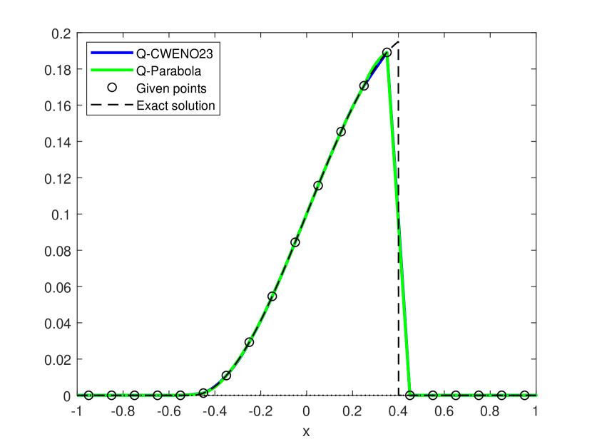
(a) Comparison of $\bar{u}_{3}$ given by (2.26) and its reconstructions.

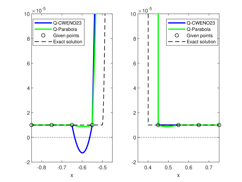
(b) Comparison of $\bar{u}_{3}$ given by (2.26) and its reconstructions on $[-0.85,-0.45]$ and $[0.35,0.75]$.

Figure 3. Comparison of reconstructions between Q-Parabola and Q-CWENO23. Dashed lines are exact solutions $\bar{u}_{3}(x)$ and black circles are given values on grid points of $\bar{u}_{3}(x)$ given in (2.26).

Summarizing, our reconstruction works as follows:

2.2.3. Algorithm for 1D case

1. Given cell average values $\{\bar{u}_{i}\}_{i\in\mathcal{I}}$ for each $i\in\mathcal{I}$, reconstruct a polynomial of even degree $k$:

   $$R_{i}(x)=\sum_{\ell=0}^{k}\frac{R_{i}^{(\ell)}}{\ell!}(x-x_{i})^{\ell}$$

   which is:

   • High order accurate in the approximation of smooth $u(x)$:

     • If $\ell$ is an even integer such that $0\leq\ell\leq k$: $\,u_{i}^{(\ell)}=R_{i}^{(\ell)}+\mathcal{O}(\Delta x^{k+2-\ell}).$

     • If $\ell$ is an odd integer such that $0\leq\ell<k$: $\,u_{i}^{(\ell)}-u_{i+1}^{(\ell)}=R_{i}^{(\ell)}-R_{i+1}^{(\ell)}+\mathcal{O}(\Delta x^{k+2-\ell}).$

   • Essentially non-oscillatory.

   • Positive preserving.

   • Conservative in the sense of cell averages: $\displaystyle\frac{1}{\Delta x}\int_{x_{i-\frac{1}{2}}}^{x_{i+\frac{1}{2}}}R_{i}(x)\,dx=\bar{u}_{i}.$

2. Using the obtained values $R_{i}^{(\ell)}$ for $0\leq\ell\leq k$, approximate $u(x_{i+\theta})$ with

   $$Q_{i+\theta}=\sum_{\ell=0}^{k}(\Delta x)^{\ell}\left(\alpha_{\ell}(\theta)R_{i}^{(\ell)}+\beta_{\ell}(\theta)R_{i+1}^{(\ell)}\right),$$

   where $\alpha_{\ell}(\theta)$ and $\beta_{\ell}(\theta)$ are given in (2.5) and (2.6)

3. Conservative reconstruction in 2D

In this section, we introduce the conservative reconstruction technique in two space dimensions, following the one adopted in the previous section. Let $u:\mathbb{R}^{2}\rightarrow\mathbb{R}$ be a smooth function and $\bar{u}:\mathbb{R}^{2}\rightarrow\mathbb{R}$ be a corresponding sliding average function:

$$\bar{u}(x,y)=\frac{1}{\Delta x\Delta y}\int_{y-\Delta y/2}^{y+\Delta y/2}\int_{x-\Delta x/2}^{x+\Delta x/2}u(x,y)\,dx\,dy.$$

Given cell averages on grid points,

$$\frac{1}{\Delta x\Delta y}\int_{I_{i,j}}u(x)\,dx=\bar{u}_{i,j},\quad I_{i,j}=[x_{i-\frac{1}{2}},x_{i+\frac{1}{2}}]\times[y_{j-\frac{1}{2}},y_{j+\frac{1}{2}}],$$

for each $(i,j)\in\mathcal{I}$, our goal is to approximate the function $\bar{u}(x,y)$. Assume we have a piecewise polynomial reconstruction $R(x,y)=\sum_{i,j}R_{i,j}(x,y)\chi_{i,j}(x,y)$, for $(i,j)\in\mathcal{I}$, where $\chi_{i,j}(x,y)$ is the characteristic function of cell $I_{i,j}$ and each $R_{i,j}(x,y)$ denotes a polynomial of degree $k$ and has the following properties:

1. It is high order accurate in the approximation of $u(x,y)$:

   (3.1) $$u(x,y)=R_{i,j}(x,y)+\mathcal{O}\left(h^{k+1}\right),\quad(x,y)\in I_{i,j},$$

   where $\Delta x,\Delta y=\mathcal{O}(h)$.

2. It is conservative in the sense of cell averages:

   $$\frac{1}{\Delta x\Delta y}\int_{y_{j-\frac{1}{2}}}^{y_{j+\frac{1}{2}}}\int_{x_{i-\frac{1}{2}}}^{x_{i+\frac{1}{2}}}R_{i,j}(x,y)\,dx\,dy=\bar{u}_{i,j}.$$

We start from a polynomial of degree $k$, $R_{i,j}(x,y)$:

(3.2) $$R_{i,j}(x,y)=\sum_{|\ell|=0}^{k}\frac{R_{i,j}^{(\ell)}}{\ell_{1}!\ell_{2}!}(x-x_{i})^{\ell_{1}}(y-y_{j})^{\ell_{2}},$$

where we use a multi index $\ell=(\ell_{1},\ell_{2})$.

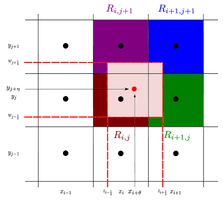
Figure 4. Description of two-dimensional conservative reconstruction

Consider a cell $I_{i,j}^{\theta,\eta}$ whose center is $(x_{i+\theta},y_{j+\eta})$ for some $\theta,\eta\in[0,1)$. In Fig. 4, we note that $(x_{i+\theta},y_{j+\eta})$ lies inside one of $I_{i,j},I_{i+1,j},I_{i,j+1},I_{i+1,j+1}$. Let us denote a cell $I_{i+\theta,j+\eta}:=[z_{i-\frac{1}{2}},z_{i+\frac{1}{2}}]\times[w_{j-\frac{1}{2}},w_{j+\frac{1}{2}}]$ and a point $(x_{i+\theta},y_{j+\eta}):=(x_{i}+\theta\Delta x,y_{j}+\eta\Delta y)$. Now, we approximate $\bar{u}(x_{i+\theta},y_{j+\eta})$ by

$$\bar{u}(x_{i+\theta},y_{j+\eta}) \approx\frac{1}{\Delta x\Delta y}\int_{w_{j-\frac{1}{2}}}^{w_{j+\frac{1}{2}}}\int_{z_{i-\frac{1}{2}}}^{z_{i+\frac{1}{2}}}R(x,y)\,dx\,dy$$

$$=\frac{1}{\Delta x\Delta y}\int_{w_{j-\frac{1}{2}}}^{y_{j+\frac{1}{2}}}\int_{z_{i-\frac{1}{2}}}^{x_{i+\frac{1}{2}}}R_{i,j}(x,y)\,dx\,dy+\frac{1}{\Delta x\Delta y}\int_{w_{j-\frac{1}{2}}}^{y_{j+\frac{1}{2}}}\int_{x_{i+\frac{1}{2}}}^{z_{i+\frac{1}{2}}}R_{i+1,j}(x,y)\,dx\,dy$$

$$+\frac{1}{\Delta x\Delta y}\int_{y_{j+\frac{1}{2}}}^{w_{j+\frac{1}{2}}}\int_{z_{i-\frac{1}{2}}}^{x_{i+\frac{1}{2}}}R_{i,j+1}(x,y)\,dx\,dy+\frac{1}{\Delta x\Delta y}\int_{y_{j+\frac{1}{2}}}^{w_{j+\frac{1}{2}}}\int_{x_{i+\frac{1}{2}}}^{z_{i+\frac{1}{2}}}R_{i+1,j+1}(x,y)\,dx\,dy.$$

The first integral becomes

$$\frac{1}{\Delta x\Delta y}\int_{w_{j-\frac{1}{2}}}^{y_{j+\frac{1}{2}}}\int_{z_{i-\frac{1}{2}}}^{x_{i+\frac{1}{2}}}R_{i,j}(x,y)\,dx\,dy =\frac{1}{\Delta x\Delta y}\sum_{|\ell|=0}^{k}R_{i,j}^{(\ell)}\int_{y_{j-\frac{1}{2}+\eta}}^{y_{j+\frac{1}{2}}}\int_{x_{i-\frac{1}{2}+\theta}}^{x_{i+\frac{1}{2}}}\frac{1}{\ell_{1}!\ell_{2}!}(x-x_{i})^{\ell_{1}}(y-y_{j})^{\ell_{2}}\,dx\,dy$$

$$=\sum_{|\ell|=0}^{k}R_{i,j}^{(\ell)}\left(\frac{1}{\Delta x}\int_{x_{i-\frac{1}{2}+\theta}}^{x_{i+\frac{1}{2}}}\frac{(x-x_{i})^{\ell_{1}}}{\ell_{1}!}\,dx\right)\left(\frac{1}{\Delta y}\int_{y_{j-\frac{1}{2}+\eta}}^{y_{j+\frac{1}{2}}}\frac{(y-y_{j})^{\ell_{2}}}{\ell_{2}!}\,dy\right)$$

$$=\sum_{|\ell|=0}^{k}(\Delta)^{\ell}\alpha_{\ell_{1}}(\theta)\alpha_{\ell_{2}}(\eta)R_{i,j}^{(\ell)}$$

where $(\Delta)^{\ell}=(\Delta x)^{\ell_{1}}(\Delta y)^{\ell_{2}}$. Similarly, we obtain

$$\frac{1}{\Delta x\Delta y}\int_{w_{j-\frac{1}{2}}}^{y_{j+\frac{1}{2}}}\int_{x_{i+\frac{1}{2}}}^{z_{i+\frac{1}{2}}}R_{i+1,j}(x,y)\,dx\,dy =\sum_{|\ell|=0}^{k}(\Delta)^{\ell}\beta_{\ell_{1}}(\theta)\alpha_{\ell_{2}}(\eta)R_{i+1,j}^{(\ell)},$$

$$\frac{1}{\Delta x\Delta y}\int_{y_{j+\frac{1}{2}}}^{w_{j+\frac{1}{2}}}\int_{z_{i-\frac{1}{2}}}^{x_{i+\frac{1}{2}}}R_{i,j+1}(x,y)\,dx\,dy =\sum_{|\ell|=0}^{k}(\Delta)^{\ell}\alpha_{\ell_{1}}(\theta)\beta_{\ell_{2}}(\eta)R_{i,j+1}^{(\ell)},$$

$$\frac{1}{\Delta x\Delta y}\int_{y_{j+\frac{1}{2}}}^{w_{j+\frac{1}{2}}}\int_{x_{i+\frac{1}{2}}}^{z_{i+\frac{1}{2}}}R_{i+1,j+1}(x,y)\,dx\,dy =\sum_{|\ell|=0}^{k}(\Delta)^{\ell}\beta_{\ell_{1}}(\theta)\beta_{\ell_{2}}(\eta)R_{i+1,j+1}^{(\ell)}.$$

Denoting the approximation of $\bar{u}(x_{i+\theta},y_{j+\theta})$ by $Q_{i+\theta,j+\eta}$, we write it as

(3.3) $$\begin{split}Q_{i+\theta,j+\eta}=\sum_{|\ell|=0}^{k}(\Delta)^{\ell}&\bigg{(}\alpha_{\ell_{1}}(\theta)\alpha_{\ell_{2}}(\eta)R_{i,j}^{(\ell)}+\beta_{\ell_{1}}(\theta)\alpha_{\ell_{2}}(\eta)R_{i+1,j}^{(\ell)}\cr&+\alpha_{\ell_{1}}(\theta)\beta_{\ell_{2}}(\eta)R_{i,j+1}^{(\ell)}+\beta_{\ell_{1}}(\theta)\beta_{\ell_{2}}(\eta)R_{i+1,j+1}^{(\ell)}\bigg{)},\end{split}$$

where the explicit forms of $\alpha_{\ell_{1}}(\theta)$, $\alpha_{\ell_{2}}(\eta)$, $\beta_{\ell_{1}}(\theta)$, $\beta_{\ell_{2}}(\eta)$ are given in (2.5) and (2.6).

3.1. General Properties

In the following proposition, as in Proposition 2.3, we show that the approximation $Q_{i+\theta,j+\eta}$ is of order $(k+2)$ of accuracy for an even integer $k\geq 0$. For simplicity, we assume $\Delta x,\Delta y=h>0.$

Proposition 3.1.

Let $k\geq 0$ be an even integer and $u$ be smooth enough so that a piecewise polynomial $R(x,y)=\sum_{i,j}R_{i,j}(x,y)\chi_{i,j}$ satifies

(3.4) $$\begin{split}u_{i,j}^{(\ell)}&=R_{i,j}^{(\ell)}+\mathcal{O}(h^{k+2-|\ell|}),\quad\text{$\ell\in A$}\cr u_{i,j}^{(\ell)}-u_{i+1,j}^{(\ell)}&=R_{i,j}^{(\ell)}-R_{i+1,j}^{(\ell)}+\mathcal{O}(h^{k+2-|\ell|}),\quad\text{$\ell\in B$}\cr u_{i,j}^{(\ell)}-u_{i,j+1}^{(\ell)}&=R_{i,j}^{(\ell)}-R_{i,j+1}^{(\ell)}+\mathcal{O}(h^{k+2-|\ell|}),\quad\text{$\ell\in C$}\end{split}$$

where the set $A,B$ and $C$ are defined

(3.5) $$\begin{split}A&=\{\ell:|\ell|=\text{even},\quad 0\leq|\ell|\leq k\},\cr B&=\{\ell:\ell_{1}=\text{odd},\quad\ell_{2}=\text{even},\quad 0\leq|\ell|\leq k\},\cr C&=\{\ell:\ell_{1}=\text{even},\quad\ell_{2}=\text{odd},\quad 0\leq|\ell|\leq k\}.\end{split}$$

Then the reconstruction $Q_{i+\theta,j+\eta}$ gives a $(k+2)$-th-order approximation of sliding averages $\bar{u}_{i+\theta,j+\eta}$ for any $\theta,\eta\in[0,1).$

Proof.

For detailed proof, see F. ∎

The conservation property also holds in the 2D reconstruction (3.3):

Proposition 3.2.

Assume that $R_{i,j}(x,y)$ satisfies

$$\frac{1}{\Delta x\Delta y}\int_{y_{j-\frac{1}{2}}}^{y_{j+\frac{1}{2}}}\int_{x_{i-\frac{1}{2}}}^{x_{i+\frac{1}{2}}}R_{i,j}(x,y)\,dx\,dy=\bar{u}_{i,j},\quad(i,j)\in\mathcal{I}.$$

Then, for periodic functions $\bar{u}(x,y)$ with period $(L,L)=(Nh,Nh),\,N\in\mathbb{N}$

$$\sum_{1\leq i,j\leq N}Q_{i+\theta,j+\theta}=\sum_{1\leq i,j\leq N}\bar{u}_{i,j},$$

for any $\theta,\eta\in[0,1)$.

Proof.

The proof is similar to the one dimensional case. ∎

3.1.1. Algorithm for 2D case

1. Given cell average values $\{\bar{u}_{i,j}\}_{(i,j)\in\mathcal{I}}$ for each $(i,j)\in\mathcal{I}$, reconstruct a polynomial of degree $k$:

   $$R_{i,j}(x,y)=\sum_{|\ell|=0}^{k}\frac{R_{i,j}^{(\ell)}}{\ell_{1}!\ell_{2}!}(x-x_{i})^{\ell_{1}}(y-y_{j})^{\ell_{2}}$$

   which is:

   • High order accurate in the approximation of $u(x)$:

     $$\begin{split}u_{i,j}^{(\ell)}&=R_{i,j}^{(\ell)}+\mathcal{O}(h^{k+2-|\ell|}),\quad\text{$\ell\in A$}\cr u_{i,j}^{(\ell)}-u_{i+1,j}^{(\ell)}&=R_{i,j}^{(\ell)}-R_{i+1,j}^{(\ell)}+\mathcal{O}(h^{k+2-|\ell|}),\quad\text{$\ell\in B$}\cr u_{i,j}^{(\ell)}-u_{i,j+1}^{(\ell)}&=R_{i,j}^{(\ell)}-R_{i,j+1}^{(\ell)}+\mathcal{O}(h^{k+2-|\ell|}),\quad\text{$\ell\in C$}\end{split}$$

     where sets $A,B,C$ are defined in (3.5).

   • Essentially non-oscillatory.

   • Positive preserving.

   • Conservative in the sense of cell averages: $\displaystyle\frac{1}{\Delta x\Delta y}\int_{y_{j-\frac{1}{2}}}^{y_{j+\frac{1}{2}}}\int_{x_{i-\frac{1}{2}}}^{x_{i+\frac{1}{2}}}R_{i,j}(x,y)\,dx\,dy=\bar{u}_{i,j}.$

2. Using the obtained values $R_{i,j}^{(\ell)}$ for $0\leq|\ell|\leq k$, approximate $\bar{u}(x_{i+\theta},y_{j+\eta})$ with

   $$Q_{i+\theta,j+\eta}=\sum_{|\ell|=0}^{k}(\Delta)^{\ell} \bigg{(}\alpha_{\ell_{1}}(\theta)\alpha_{\ell_{2}}(\eta)R_{i,j}^{(\ell)}+\beta_{\ell_{1}}(\theta)\alpha_{\ell_{2}}(\eta)R_{i+1,j}^{(\ell)}$$

   $$+\alpha_{\ell_{1}}(\theta)\beta_{\ell_{2}}(\eta)R_{i,j+1}^{(\ell)}+\beta_{\ell_{1}}(\theta)\beta_{\ell_{2}}(\eta)R_{i+1,j+1}^{(\ell)}\bigg{)},$$

   where $\alpha_{\ell_{1}}(\theta)$, $\alpha_{\ell_{2}}(\eta)$, $\beta_{\ell_{1}}(\theta)$, $\beta_{\ell_{2}}(\eta)$ are computable using (2.5) and (2.6).

4. Semi-Lagrangian schemes for hyperbolic systems with relaxation

In this section, as an application of the conservative reconstruction (2.7) and (3.3), we consider semi-Lagrangian methods to semi-linear hyperbolic relaxation systems. Two semi-linear hyperbolic relaxation system, namely, Xin-Jin system [23] and Broadwell model [3], where a relaxation parameter $\kappa$ makes each system stiff as $\kappa\to 0$.

In order to treat the stiffness, we shall use L-stable $s$-stage DIRK methods or L-stable linear multi-step methods (in particular BDF methods) [20]. These methods provide a balanced performance between stability and efficiency.

From now on, we focus on L-stable $s$-stage DIRK methods represented by Butcher’s tables:

$$\begin{array}[]{c|c}c&A\\ \hline\cr&b^{T}\end{array}$$

where $A=[a_{k\ell}]$ is a $s\times s$ lower triangle matrix such that $a_{k\ell}=0$ for $\ell>k$, $c=(c_{1},...,c_{s})^{T}$ and $b=(b_{1},...,b_{s})^{T}$ are coefficient vectors. (For BDF based methods, we refer to G.1.)

In order to guarantee L-stability, here we make use of stiffly accurate schemes (SA), i.e. schemes for which the last row of matrix A is equal to the vector of weights $a_{sj}=b_{j}$, $j=1,...,s$. This will ensure that the absolute stability function vanishes at infinity. As a consequence, an A-stable scheme which is SA is also L-stable, [20].

In the numerical tests for each order of accuracy, we will use the following high-order L-stable DIRK methods:

• second-order DIRK method (DIRK2) [21],

  (4.4) $$\begin{array}[]{c|c c}\alpha&\alpha&0\\ 1&1-\alpha&\alpha\\ \hline\cr&1-\alpha&\alpha\end{array},\quad\alpha=1-\frac{\sqrt{2}}{2}.$$

• third-order DIRK method (DIRK43) [25],

  (4.5) $$\begin{split}\begin{array}[]{c|c c c c}0&0&0&0&0\\[4.2679pt] \displaystyle 2\gamma&\displaystyle\gamma&\displaystyle\gamma&0&0\\[4.2679pt] \displaystyle c&\displaystyle c-\delta-\gamma&\displaystyle\delta&\displaystyle\gamma&0\\[4.2679pt] 1&\displaystyle 1-b_{2}-b_{3}-\gamma&\displaystyle b_{2}&\displaystyle b_{3}&\displaystyle\gamma\\[4.2679pt] \hline\cr\\ &\displaystyle 1-b_{2}-b_{3}-\gamma&\displaystyle b_{2}&\displaystyle b_{3}&\displaystyle\gamma\\ \end{array}\end{split}$$

with $\displaystyle\gamma=\frac{1767732205903}{4055673282236}\,$, $\displaystyle c=\frac{3}{5}\,$, $\displaystyle b_{2}=-\frac{4482444167858}{7529755066697}\,$, $\displaystyle b_{3}=\frac{11266239266428}{11593286722821}\,$, $\displaystyle\delta=-\frac{640167445237}{6845629431997}$.

4.1. Xin-Jin relaxation system

Consider a simplified Xin-Jin relaxation system [23]:

(4.6) $$\begin{split}\frac{\partial u}{\partial t}+\sum_{i=1}^{d}\frac{\partial v}{\partial{x_{i}}}&=0,\cr\frac{\partial v}{\partial t}+a^{2}\sum_{i=1}^{d}\frac{\partial u}{\partial{x_{i}}}&=\frac{1}{\kappa}(F(u)-v),\cr\end{split}$$

where $d$ denotes the dimension of space variable. When $\kappa$ goes to zero, the solution in (4.6) converges to

(4.7) $$\frac{\partial u}{\partial t}+\sum_{i=1}^{d}\frac{\partial F(u)}{\partial{x_{i}}}=0,\quad v=F(u).$$

provided that the subcharacteristic condition is satisfied, i.e., $\max_{u}{|F^{\prime}(u)|}\leq|a|$ (see [11]). For example, taking $F(u)=u^{2}/2$, the system (4.7) formally becomes the Burgers equation:

(4.8) $$\frac{\partial u}{\partial{t}}+\sum_{i=1}^{d}u\frac{\partial u}{\partial{x_{i}}}=0,\quad v=\frac{u^{2}}{2}.$$

In this equation, shocks may appear in a finite time and we need to impose our scheme to be conservative to capture the positions of such shocks correctly. We treat this shock problem in section 5.

4.1.1. Semi-Lagrangian scheme for Xin-Jin relaxation system

Using $u-v=f$ and $u+v=g$, we rewrite (4.6) as

(4.9) $$\begin{split}\frac{\partial f}{\partial{t}}-\sum_{i=1}^{d}\frac{\partial f}{\partial{x_{i}}}&=-\frac{1}{\kappa}\left[F\left(\frac{g+f}{2}\right)-\frac{g-f}{2}\right]\cr\frac{\partial g}{\partial{t}}+\sum_{i=1}^{d}\frac{\partial g}{\partial{x_{i}}}&=-\frac{1}{\kappa}\left[\frac{g-f}{2}-F\left(\frac{g+f}{2}\right)\right].\end{split}$$

Based on this, we consider its Lagrangian formulation:

(4.10) $$\begin{split}\frac{df}{dt}(X_{1}(t),t)&=-\frac{1}{\kappa}\left[F\left(\frac{g+f}{2}\right)-\frac{g-f}{2}\right](X_{1}(t),t),\quad\frac{dX_{1}}{dt}=-\mathbbm{1}\cr\frac{dg}{dt}(X_{2}(t),t)&=-\frac{1}{\kappa}\left[\frac{g-f}{2}-F\left(\frac{g+f}{2}\right)\right](X_{2}(t),t),\quad\frac{dX_{2}}{dt}=\mathbbm{1},\end{split}$$

where $\mathbbm{1}=(1,\cdots,1)\in\mathbb{N}^{d}$ and $X_{1}(t^{n+1})=X_{2}(t^{n+1})=x_{i}\in\mathbb{R}^{d}$.

To clarify high order methods for (4.10), we introduce the following notation:

• The $\ell$-th stage values of $f,g$ along the backward-characteristics which come from $x_{i}$ with characteristic speed $-1,1$ at time $t^{n}+c_{k}\Delta t$:

  $$\tilde{f}_{i}^{(k,\ell)} \approx f(x_{i}+(c_{k}-c_{\ell})\Delta t,t^{n}+c_{\ell}\Delta t),\quad\tilde{g}_{i}^{(k,\ell)}\approx f(x_{i}-(c_{k}-c_{\ell})\Delta t,t^{n}+c_{\ell}\Delta t)$$

  where ”$\approx$” implies the necessity of suitable reconstructions. We also denote $k$-th stage value of $f,g$ on $x_{i}$ by

  $$f_{i}^{(k)} =f(x_{i},t^{n}+c_{k}\Delta t),\quad g_{i}^{(k)}=g(x_{i},t^{n}+c_{k}\Delta t)$$

  for $1\leq k\leq s$ where $f_{i}^{(k)}=u_{i}^{(k)}-v_{i}^{(k)}$ and $g_{i}^{(k)}=u_{i}^{(k)}+v_{i}^{(k)}$.

• For $\ell=0$, we set $c_{\ell}=0$ hence

  (4.11) $$\tilde{f}_{i}^{(k,0)}\approx f(x_{i}+c_{k}\Delta t,t^{n}),\quad\tilde{g}_{i}^{(k,0)}\approx g(x_{i}-c_{k}\Delta t,t^{n}).$$

• Define a RK flux function by $K_{1}:=F(u)-v$, $K_{2}:=-K_{1}$, then

  $$K_{i,j}^{(k,\ell)}\approx K_{j}(x_{i}-\lambda_{j}(c_{k}-c_{\ell})\Delta t,t^{n}+c_{\ell}\Delta t),\quad j=1,2$$

  where $\lambda_{1}=-1,\lambda_{2}=1$ and $K_{i,j}^{(k)}=K_{j}(x_{i},t^{n}+c_{k}\Delta t)$.

With these, we can represent a high order method compactly. Applying a L-stable $s$-stage DIRK method to system (4.10), we have $k$-stage values

(4.12) $$\begin{split}f_{i}^{(k)}&=\tilde{f}_{i}^{(k,0)}-\frac{\Delta t}{\kappa}\sum_{\ell=1}^{s}a_{k\ell}K_{i,1}^{(k,\ell)},\cr g_{i}^{(k)}&=\tilde{g}_{i}^{(k,0)}-\frac{\Delta t}{\kappa}\sum_{\ell=1}^{s}a_{k\ell}K_{i,2}^{(k,\ell)},\end{split}$$

for $k=1,\dots,s$. Since we only consider SA DIRK schemes, the $s$-stage values become the numerical solutions: $f^{n+1}_{i}=f_{i}^{(s)}$ and $g^{n+1}_{i}=g_{i}^{(s)}$. It is worth mentioning that each $k$-stage value can be computed in an explicit way. After summing and subtracting two equations in (4.12), we obtain

(4.13) $$\begin{split}u_{i}^{(k)}&=\frac{\tilde{g}_{i}^{(k,0)}+\tilde{f}_{i}^{(k,0)}}{2}-\frac{\Delta t}{2\kappa}\sum_{\ell=1}^{k-1}a_{k\ell}\left(K_{i,1}^{(k,\ell)}+K_{i,2}^{(k,\ell)}\right),\cr v_{i}^{(k)}&=\frac{\tilde{g}_{i}^{(k,0)}-\tilde{f}_{i}^{(k,0)}}{2}-\frac{\Delta t}{2\kappa}\left(\sum_{\ell=1}^{k-1}a_{k\ell}\left(K_{i,2}^{(k,\ell)}-K_{i,1}^{(k,\ell)}\right)\right)+\frac{a_{kk}\Delta t}{\kappa}\left(F(u_{i}^{(k)})-v_{i}^{(k)}\right).\end{split}$$

Here we first compute $u_{i}^{(k)}$, and use it obtain $v_{i}^{(k)}$. Now we illustrate our L-stable DIRK schemes as follows: (A schematic for DIRK2 based scheme is given in Fig 5.)

Figure 5. Schematic of DIRK2 based SL method for Xin-Jin model. Gray circles are points where reconstruction is required.

4.1.2. Algorithm of $s$-stage L-stable DIRK method

For $k=1,\dots,s$.

1. Interpolate $\tilde{f}_{i}^{(k,0)}$ and $\tilde{g}_{i}^{(k,0)}$ on $x_{i}+c_{k}\Delta t$ and $x_{i}-c_{k}\Delta t$ from $\{f_{i}^{n}\}$ and $\{g_{i}^{n}\}$, respectively.

2. Compute $u_{i}^{(k)}$ and $v_{i}^{(k)}$ from (4.13).

3. Compute:

   (4.14) $$f_{i}^{(k)}=u_{i}^{(k)}-v_{i}^{(k)},\quad g_{i}^{(k)}=u_{i}^{(k)}+v_{i}^{(k)}$$

4. If $k<s$, compute

   $$K_{i,1}^{(k)} =F(u_{i}^{(k)})-v_{i}^{(k)},\quad K_{i,2}^{(k)}=-K_{i,1}^{(k)}$$

   and, for $\ell=k+1,\cdots,s$, interpolate

   $$\text{$K_{i,1}^{(\ell,k)}$ on $x_{i}+(c_{\ell}-c_{k})\Delta t$ from $\{K_{i,1}^{(k)}\}$},$$

   $$\text{$K_{i,2}^{(\ell,k)}$ on $x_{i}-(c_{\ell}-c_{k})\Delta t$ from $\{K_{i,2}^{(k)}\}$}.$$

5. Compute numerical solution: $f^{n+1}_{i}=f_{i}^{(s)}$ and $g^{n+1}_{i}=g_{i}^{(s)}$.

For any term where reconstruction is required, we use the formula (2.7) based on the CWENO reconstructions.

Remark 4.1.

In the Algorithm 4.1.2, using the implicit Euler method for $s=1$ and taking a limit $\kappa\to 0$ in (4.13), we obtain

(4.15) $$u_{i}^{n+1} =\frac{\tilde{g}_{i}^{(1,0)}+\tilde{f}_{i}^{(1,0)}}{2},\quad v_{i}^{n+1}=F(u_{i}^{n+1}),$$

for all $n\geq 0$ regardless of initial data. Now assume that $\Delta t=\Delta x$, and we combine (4.15) with (4.11), and (4.14) for $k=1$ obtaining

$$\begin{split}u_{i}^{n+1}&=\frac{1}{2}\left(u_{i+1}^{n}+u_{i-1}^{n}\right)-\frac{1}{2}\left(F\left(u_{i+1}^{n}\right)-F\left(u_{i-1}^{n}\right)\right).\end{split}$$

This is the Lax–Friedrichs method of the conservation law in (4.7) with $\Delta t=\Delta x$.

4.2. Broadwell model

Next example is the Broadwell model of kinetic theory [3]:

(4.16) $$\begin{split}\partial_{t}f+\partial_{x}f&=\frac{1}{\kappa}Q\cr\partial_{t}g-\partial_{x}g&=\frac{1}{\kappa}Q\cr\partial_{t}h&=-\frac{1}{\kappa}Q.\end{split}$$

where $Q=h^{2}-fg$. Introducing the fluid dynamic moment variables dentity $\rho$, momentum $m$, and velocity $u$ and an additional variable $z$ as follows:

(4.17) $$\rho=f+2h+g,\quad m=f-g,\quad z=f+g,$$

the system (4.16) can be rewritten as

(4.18) $$\begin{split}&\partial_{t}\rho+\partial_{x}m=0\cr&\partial_{t}m+\partial_{x}z=0\cr&\partial_{t}z+\partial_{x}m=\frac{1}{2\kappa}\left(\rho^{2}-2\rho z+m^{2}\right).\end{split}$$

Note that the original variables can be recovered by

$$f=\frac{z+m}{2},\quad g=\frac{z-m}{2},\quad h=\frac{\rho-z}{2}.$$

As $\kappa\rightarrow 0$, one can see that $z$ goes to a local equibrium

$$z\rightarrow z_{E}(\rho,m):=\frac{1}{2\rho}\left(\rho^{2}+m^{2}\right)=\frac{1}{2}\left(\rho+\rho u^{2}\right)$$

and the system (4.18) becomes the Euler equations:

(4.19) $$\begin{split}&\partial_{t}\rho+\partial_{x}m=0\cr&\partial_{t}m+\partial_{x}\left(\frac{1}{2}\left(\rho+\rho u^{2}\right)\right)=0.\end{split}$$

4.2.1. Semi-Lagrangian scheme for the Broadwell model

Here, we consider again DIRK methods based on Tables (4.4)-(4.5). The schemes are also explicitly solvable with algebraic computations. (For BDF methods, we refer to (G.2).)

Let us denote $k$-th stage values by $f_{i}^{(k)}$, $g_{i}^{(k)}$, $h_{i}^{(k)}$, $1\leq k\leq s$, and introduce the following notation:

$$Q_{i}^{(k)} =(h_{i}^{(k)})^{2}-f_{i}^{(k)}g_{i}^{(k)},$$

$$Q_{i,1}^{(k,\ell)} \approx Q(x_{i}-(c_{k}-c_{\ell})\Delta t,t^{n}+c_{\ell}\Delta t),\quad Q_{i,2}^{(k,\ell)}\approx Q(x_{i}+(c_{k}-c_{\ell})\Delta t,t^{n}+c_{\ell}\Delta t),$$

$$f_{i}^{(k,\ell)} \approx f(x_{i}-(c_{k}-c_{\ell})\Delta t,t^{n}+c_{\ell}\Delta t),\quad g_{i}^{(k,\ell)}\approx g(x_{i}-(c_{k}-c_{\ell})\Delta t,t^{n}+c_{\ell}\Delta t).$$

Applying a $s$-stage DIRK method to (4.16), we can write $k$-th stage values in a compact form:

(4.20) $$\begin{split}f_{i}^{(k)}&=F_{i}^{(k)}+\frac{a_{kk}\Delta t}{\kappa}Q_{i}^{(k)},\quad F_{i}^{(k)}:=f_{i}^{(k,0)}+\frac{\Delta t}{\kappa}\sum_{\ell=1}^{k-1}a_{k\ell}Q_{i,1}^{(k,\ell)}\cr g_{i}^{(k)}&=G_{i}^{(k)}+\frac{a_{kk}\Delta t}{\kappa}Q_{i}^{(k)},\quad G_{i}^{(k)}:=g_{i}^{(k,0)}+\frac{\Delta t}{\kappa}\sum_{\ell=1}^{k-1}a_{k\ell}Q_{i,2}^{(k,\ell)}\cr h_{i}^{(k)}&=H_{i}^{(k)}-\frac{a_{kk}\Delta t}{\kappa}Q_{i}^{(k)},\quad H_{i}^{(k)}:=h_{i}^{n}-\frac{\Delta t}{\kappa}\sum_{\ell=1}^{k-1}a_{k\ell}Q_{i}^{(\ell)},\end{split}$$

for $k=1,2,\dots,s$. Here the SA property also implies $f_{i}^{n+1}=f_{i}^{(s)}$, $g_{i}^{n+1}=g_{i}^{(s)}$ and $h_{i}^{n+1}=h_{i}^{(s)}$.

Now, we describe the algorithm:

4.2.2. Algorithm of $s$-stage L-stable DIRK method

For $k=1,\cdots,s$, iterate the following procedures:

1. Reconstruct $f_{i}^{(k,0)}$ and $g_{i}^{(k,0)}$ on $x_{i}-c_{k}\Delta t$ and $x_{i}+c_{k}\Delta t$ from $\{f_{i}^{n}\}$ and $\{g_{i}^{n}\}$, respectively.

2. Reconstruct $Q_{i,1}^{(k,\ell)}$ and $Q_{i,2}^{(k,\ell)}$ for $\ell=1,\cdots,k-1$ from $\{Q_{i}^{(\ell)}\}$ (skip this if $k=1$).

3. Compute $F_{i}^{(k)}$, $G_{i}^{(k)}$ and $H_{i}^{(k)}$ using (4.20).

4. Solve

   (4.21) $$\begin{split}f_{i}^{(k)}=F_{i}^{(k)}+\frac{a_{kk}\Delta t}{\kappa}Q_{i}^{(k)},\quad g_{i}^{(k)}=G_{i}^{(k)}+\frac{a_{kk}\Delta t}{\kappa}Q_{i}^{(k)},\quad h_{i}^{(k)}=H_{i}^{(k)}-\frac{a_{kk}\Delta t}{\kappa}Q_{i}^{(k)}\end{split}$$

   for

   (4.22) $$\begin{split}&h_{i}^{(k)}=\frac{a_{kk}\Delta t(H_{i}^{(k)}+F_{i}^{(k)})(H_{i}^{(k)}+G_{i}^{(k)})+\kappa H_{i}^{(k)}}{a_{kk}\Delta t\left(G_{i}^{(k)}+2H_{i}^{(k)}+F_{i}^{(k)}\right)+\kappa},\cr&f_{i}^{(k)}=H_{i}^{(k)}+F_{i}^{(k)}-h_{i}^{(k)},\qquad g_{i}^{(k)}=H_{i}^{(k)}+G_{i}^{(k)}-h_{i}^{(k)}.\end{split}$$

Remark 4.2.

In Algorithm 4.2.2, consider the case $s=1$ for implicit Euler method. Under the assumption $\Delta t=\Delta x$, the relaxation limit $\kappa\to 0$ in (4.22) gives

(4.23) $$\begin{split}&h_{i}^{n+1}=\frac{(h_{i}^{n}+f_{i-1}^{n})(h_{i}^{n}+g_{i+1}^{n})}{g_{i+1}^{n}+2h_{i}^{n}+f_{i-1}^{n}},\cr&f_{i}^{n+1}=h_{i}^{n}+f_{i}^{(1,0)}-h_{i}^{n+1},\qquad g_{i}^{n+1}=h_{i}^{n}+g_{i}^{(1,0)}-h_{i}^{n+1}.\end{split}$$

This limiting scheme coincides with the relaxation scheme in [24] applied to the Broadwell model. Also, using the relation (4.17), we can rewrite it as follows:

$$\rho_{i}^{n+1} =\rho_{i}^{n}-\frac{1}{2}\left(m_{i+1}^{n}-m_{i-1}^{n}\right)+\frac{1}{2}\left(z_{i-1}^{n}-2z_{i}^{n}+z_{i-1}^{n}\right),$$

$$m_{i}^{n+1} =\frac{1}{2}\left(m_{i+1}^{n}+m_{i-1}^{n}\right)-\frac{1}{2}\left(z_{i+1}^{n}-z_{i-1}^{n}\right),$$

$$z_{i}^{n+1} =\frac{(\rho_{i}^{n+1})^{2}+(m_{i}^{n+1})^{2}}{2\rho_{i}^{n+1}}.$$

We note that the scheme projects numerical solutions to equilibrium after one time step.

5. Numerical tests

Our main interest is to confirm the performance of the proposed reconstruction in one and two dimensions. For numerical experiments, we consider the reconstruction (2.7) and (3.3) based on CWENO reconstructions. This section is divided into three parts: 1D Xin-Jin model (4.6), 1D Broadwell model (4.16) and 2D Xin-Jin model (4.6). For each system, we check the accuracy of the corresponding semi-Lagrangian schemes and consider the related shock problems which arise in the relaxation limit $\kappa\rightarrow 0$. For numerical tests, we use the CFL number defined by CFL$=\frac{\Delta t}{\Delta x}$ using uniform grid points based on $\Delta x$ and $\Delta t$. For 2D, we use CFL$=\frac{\Delta t}{\Delta x}=\frac{\Delta t}{\Delta y}$.

5.1. 1D case for Xin-Jin model

Here tests are based on the numerical method in Algorithm 4.1.2. Note that we adopt $F(u)=u^{2}/2$.

5.1.1. Accuracy test

We take well-prepared initial data up to first order in $\kappa$ [2]:

(5.1) $$u_{0}(x)=0.7+0.2\sin(\pi x),\quad v_{0}(x)=\frac{u_{0}^{2}(x)}{2}+\kappa\left(u_{0}^{2}(x)-1\right)\partial_{x}u_{0}(x),$$

where periodic boundary conditions are imposed on $x\in[-1,1]$. In the limit $\kappa\rightarrow 0$ with $F(u)=u^{2}/2$, system (4.6) becomes the Burgers equation where shock appears after the positive minimum time: $\displaystyle T_{b}:=\inf_{u_{0}^{\prime}<0}\left\{-\frac{1}{u_{0}^{\prime}(x)}\right\}$. In view of this, we take a final time as $T^{f}=1$ which is less than the breaking time $T_{b}=5/\pi\approx 1.5915$. In this test, we use several values of CFL=$\Delta t/\Delta x<1$. We remark that the subcharacteristic condition $\max_{u}|F^{\prime}(u)|<1$ is always satisfied. In Fig. 6, a DIRK2 based method attains its desired accuracy between 2 and 3. In the case of DIRK43 method, it attains its desired accuracy between 3 and 5 except for some order reductions which appear in the intermediate regimes. We remark that the spatial errors are dominant for small CFL numbers, which make it easy to observe the order of spatial reconstructions.

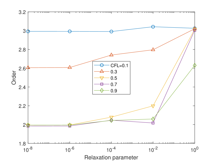
(a) DIRK2 - Q-CWENO23

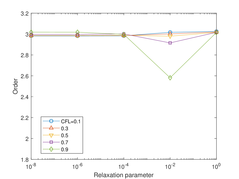
(b) DIRK43 - Q-CWENO23

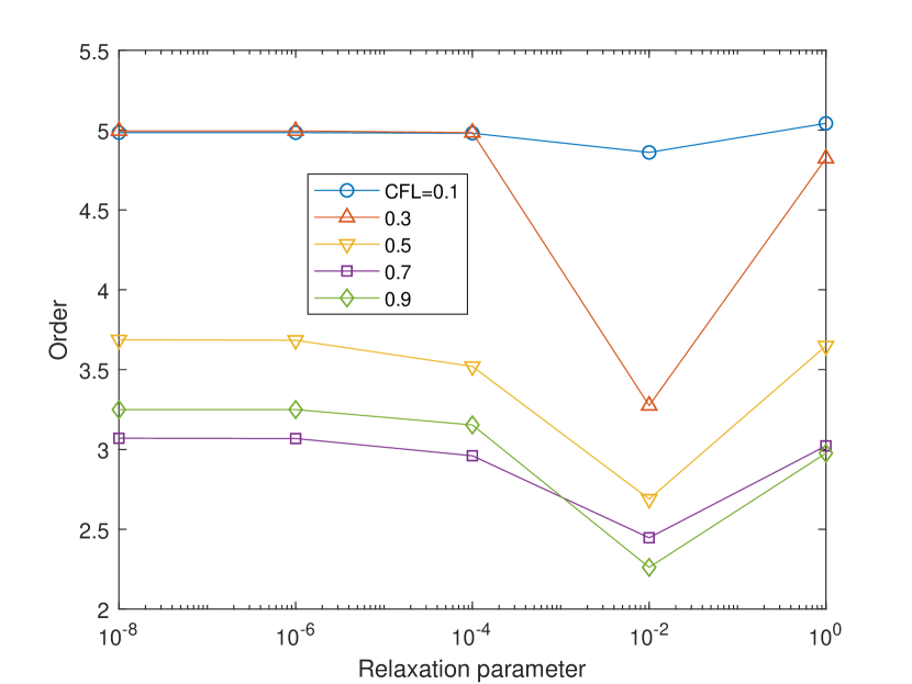
(c) DIRK43 - Q-CWENO35

Figure 6. Accuracy tests for 1D Xin-Jin model. Initial data is associated to (5.1). $x$-axis is for the relaxation parameter $\kappa$ and $y$-axis is for order of accuracy based on $N_{x}=160,320,640$.

5.1.2. Shock tests

To confirm the conservation property of the proposed reconstruction in shock problems, we here compare numerical solutions obtained by conservative semi-Lagrangian schemes with non-conservative ones.

$\bullet$ Smooth initial data. We first take the an smooth initial data

(5.2) $$u_{0}(x)=0.7+0.2\sin(\pi x),\quad v_{0}(x)=\frac{u_{0}^{2}(x)}{2},$$

where periodic boundary condition is imposed on $x\in[-1,1]$. We use grid points of $N_{x}=160$ up to final time $T^{f}=4$. Each time step is taken by $\Delta t=\text{CFL}\Delta x$. For each time $t=t^{n}$, we compute the conservation error using

$$E_{con}^{n}:=\frac{\left|\sum_{i}u_{i}^{n}\Delta x-\sum_{i}u_{i}^{0}\Delta x\right|}{\sum_{i}u_{i}^{0}\Delta x}.$$

In Fig. 7, we compare the numerical solutions obtained from our reconstruction, linear interpolation (first order scheme), GWENO34 and GWENO46 [7] with the reference solution in [36]. We observe that the use of our reconstruction and linear interpolation leads to correct shock position. Also, the corresponding conservative errors show very small change as time flows. In contrast, conservation errors become bigger when we adopt GWENO34 and GWENO46 reconstructions after time $t=1$, which give wrong shock positions. (See Fig. 7)

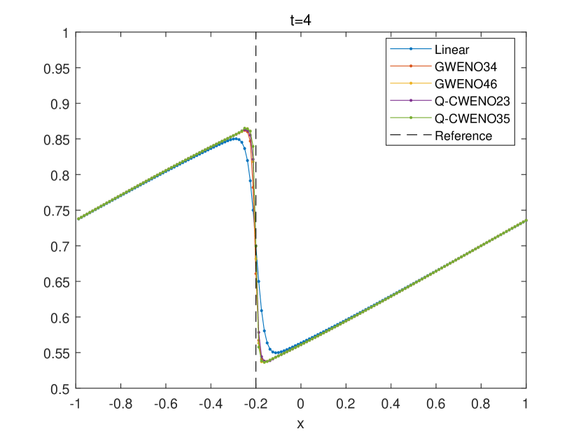
(a) Comparison of numerical solutions w.r.t. reconstruction at $x\in[-1,1]$

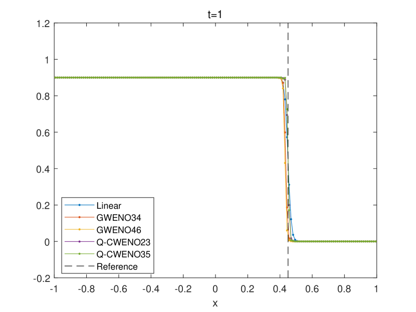
(b) Comparison of numerical solutions w.r.t. reconstruction at $x\in[-1,1]$

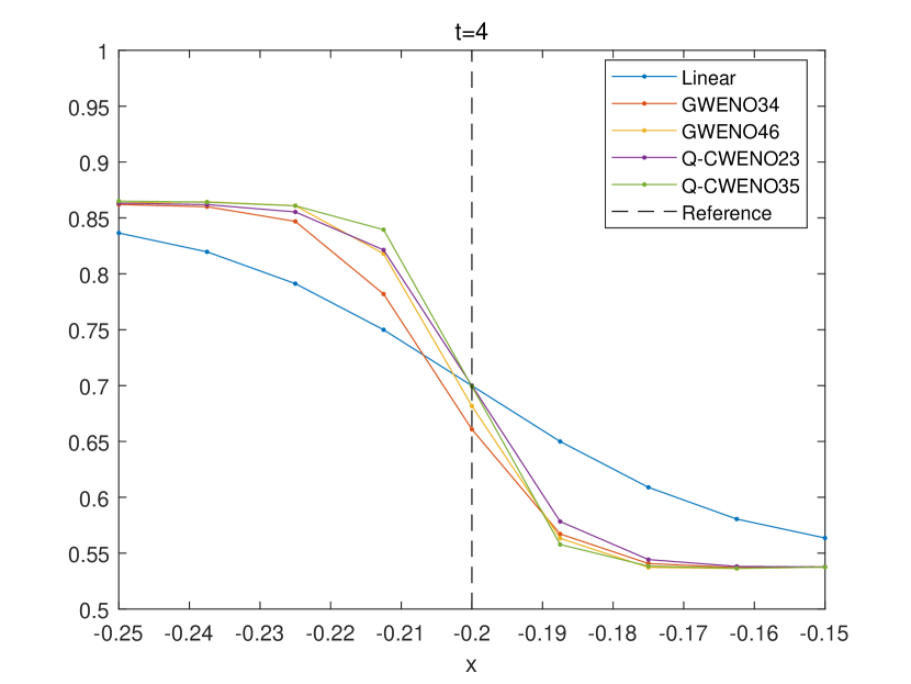
(c) Numerical solutions w.r.t. reconstruction at $x\in[-0.25,-0.15]$

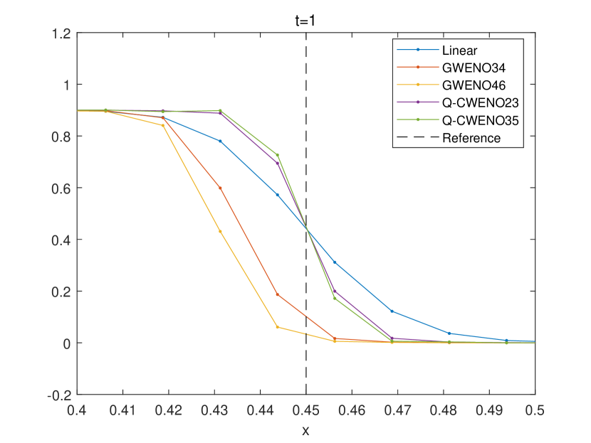
(d) Numerical solutions w.r.t. reconstruction at $x\in[0.4,0.6]$

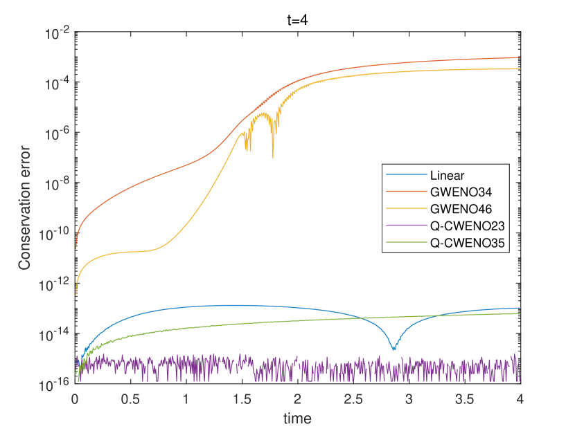
(e) Conservation errors w.r.t. time

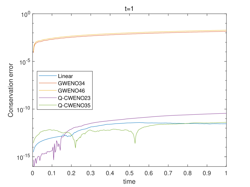
(f) Conservation errors w.r.t. time

Figure 7. Shock tests for 1D Xin-Jin model. Left: initial data (5.2) with CFL$=0.5$ Right: initial data (5.3) with CFL$=0.3$. The results are obtained by DIRK43 based SL methods for $\kappa=10^{-8}$ with various reconstructions.

$\bullet$ Discontinuous initial data. In this test, we again solve the system (4.6) with initial data

(5.3) $$u_{0}(x)=\begin{cases}0.9,\quad x\leq 0\\ 0,\quad x>0\end{cases},\quad v_{0}(x)=\frac{u_{0}^{2}(x)}{2}$$

under freeflow boundary condition on $x\in[-1,1]$ with grid points $N_{x}=160$ up to final time $T^{f}=1$. In this test, we compute the conservation error using

$$E_{con}^{n}:=\frac{\sum_{i}u_{i}^{n}\Delta x-(\sum_{i}u_{i}^{0}\Delta x+st^{n})}{\sum_{i}u_{i}^{0}\Delta x},$$

where $s$ is the speed of shock, which is given by $s=0.45$.

We show our reconstruction can be more effective in capturing shock position. In Fig. 7, we again compare the numerical solutions for different reconstructions. As in the previous shock test, our reconstruction and linear interpolation show better performance in capturing shock position compared to GWENO34 and GWENO46 reconstructions.

Remark 5.1.

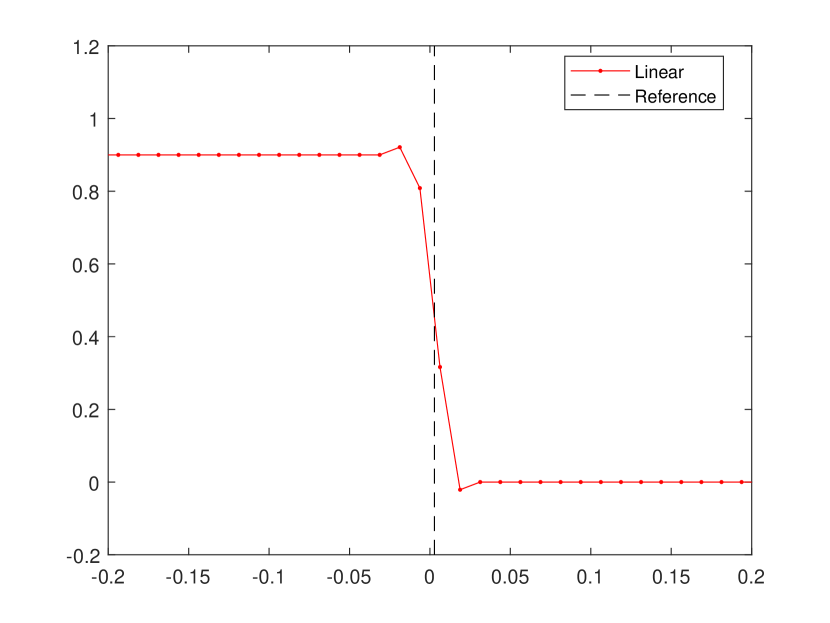
Figure 8. Shock test associated to Remark 5.1. For $\kappa=10^{-8}$, DIRK2 based SL scheme is implemented with linear interpolation. Note that oscillation appears at $T^{f}=\Delta t=0.00625$.

In the section 5.1, we confirmed that high-order DIRK based SL schemes of Xin-Jin model works for all ranges of relaxation parameters. We also observed that, in the limit $\kappa\rightarrow 0$, oscillations appear near discontinuities for all high-order RK and BDF based SL schemes. To understand this phenomena, as a simple case, consider $F(u)=bu$ for $|b|<1$. We will show that oscillation appears even after one step $t=t^{1}$ for arbitrary second order DIRK based SL schemes with linear interpolation (see Fig 8). We use the Butcher’s table given by

$$\begin{array}[]{c|c c}\alpha_{1}&\alpha_{1}&0\\ 1&1-\alpha_{2}&\alpha_{2}\\ \hline\cr&1-\alpha_{2}&\alpha_{2}\end{array},\quad\alpha_{2}=\frac{\frac{1}{2}-\alpha_{1}}{1-\alpha_{1}}.$$

Then, with the initial conditions (5.3), the following calculation verifies our remark. $\bullet$ Assume CFL$=\frac{\Delta t}{\Delta x}\leq 1$, and $(u_{i-2}^{0},u_{i-1}^{0},u_{i}^{0},u_{i+1}^{0},u_{i+2}^{0})=(0.9,0.9,0.9,0.9,0)$. Then, in the limit $\kappa\rightarrow 0$, we have

$$u_{i}^{1} =\left(1-\frac{\Delta t}{\Delta x}\right)u_{i}^{0}+\frac{\Delta t}{2\Delta x}(u_{i-1}^{0}+u_{i+1}^{0})-\frac{b\Delta t}{2\Delta x}(u_{i-1}^{0}-u_{i+1}^{0})+\frac{(b^{2}-1)(\Delta t)^{2}}{8(\Delta x)^{2}}(u_{i-2}^{0}-2u_{i}^{0}+u_{i+2}^{0})$$

$$=0.9\left(1+\frac{(1-b^{2})(\Delta t)^{2}}{8(\Delta x)^{2}}\right)>0.9,$$

for any $\alpha_{1}\neq 0,1$.

5.2. 1D Broadwell model

Now, we move on to the semi-Lagrangian schemes for 1D Broadwell model (4.16).

5.2.1. Accuracy test

To check the accuracy of the proposed schemes, we consider well-prepared data [31]:

(5.4) $$\begin{split}\rho_{0}(x)&=1+a_{\rho}\sin{\frac{2\pi}{L}x},\quad u_{0}(x)=\frac{1}{2}+a_{u}\sin{\frac{2\pi}{L}x},\cr z_{0}(x)&=z_{E}(\rho_{0}(x),u_{0}(x))+\kappa z_{1}(\rho_{0}(x),u_{0}(x))\end{split}$$

where $a_{\rho}=0.3$, $a_{u}=0.1$, $L=20$, $T^{f}=30$, and

$$z_{E}(\rho_{0},m_{0}) =\frac{1}{2\rho_{0}}\left(\rho_{0}^{2}+m_{0}^{2}\right),\quad z_{1}(\rho_{0},m_{0})=-\frac{H(\rho_{0},m_{0})}{\rho_{0}},$$

$$H(\rho_{0},m_{0}) =\left(1-\partial_{\rho}z_{E}+(\partial_{m}z_{E})^{2}\right)\partial_{x}m_{0}+(\partial_{\rho}z_{E}\partial_{m}z_{E})\partial_{x}\rho_{0}.$$

The periodic condition is imposed on $[-20,20]$ upto final time $T^{f}=30$. We take different CFL numbers less than $1$. The order of convergence is based on the grid points $N_{x}=160,320,640$. Here the desired accuracy for DIRK2 is between 2 and 3, while for DIRK43, it is between 3 and 5.

In Fig. 9, one can see that the DIRK2 based method attains the desired accuracy for all ranges of $\kappa$. On the other hand, in the limit $\kappa\rightarrow 0$, the DIRK43 based method shows order reduction, which could be prevented by adopting the BDF3 based method. For small CFL numbers, space errors dominate so the order of accuracy comes from spatial reconstruction, while for large CFL time discretization errors dominate so the order of accuracy comes from time integration.

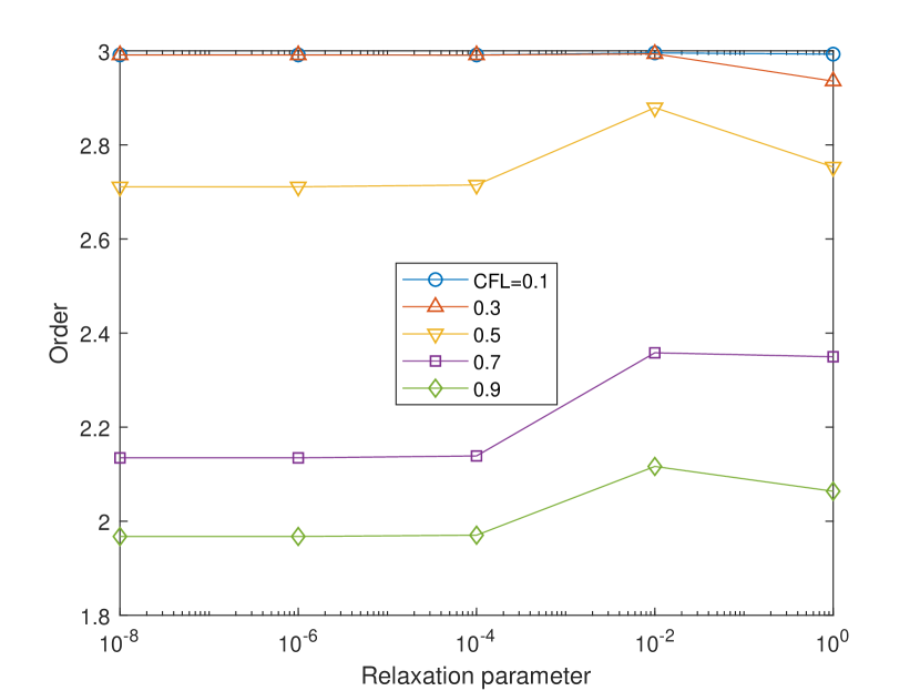
(a) DIRK2, Q-CWENO23

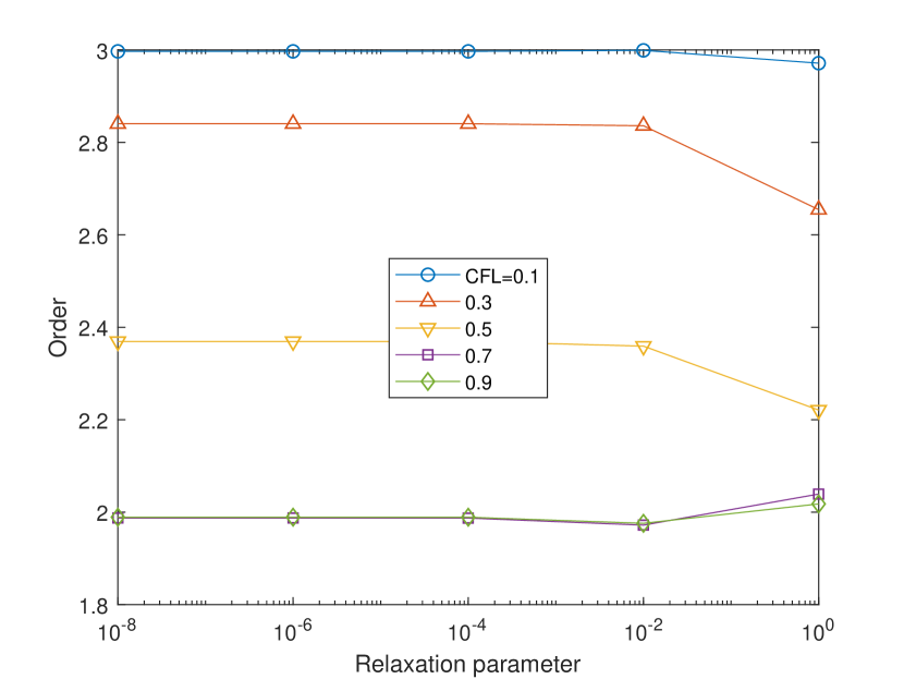
(b) BDF2, Q-CWENO23

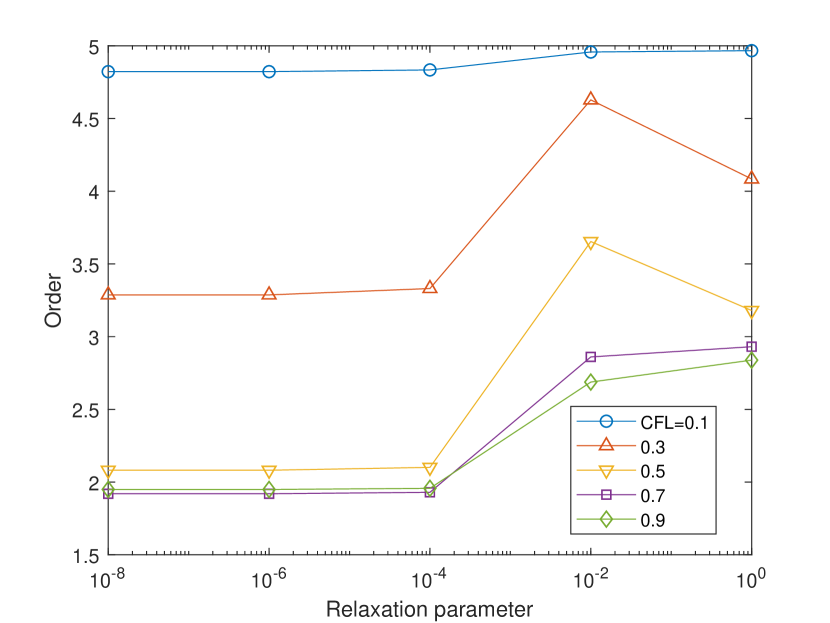
(c) DIRK43, Q-CWENO35

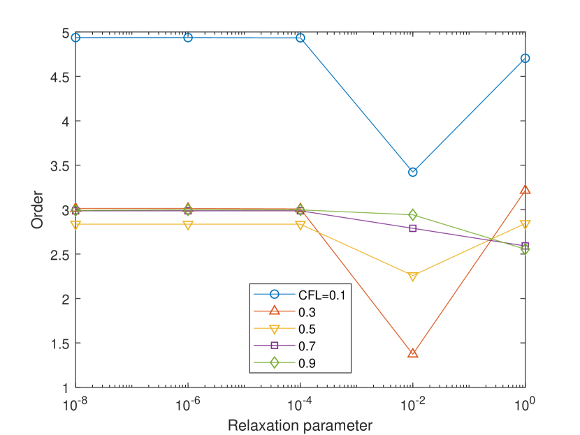
(d) BDF3, Q-CWENO35

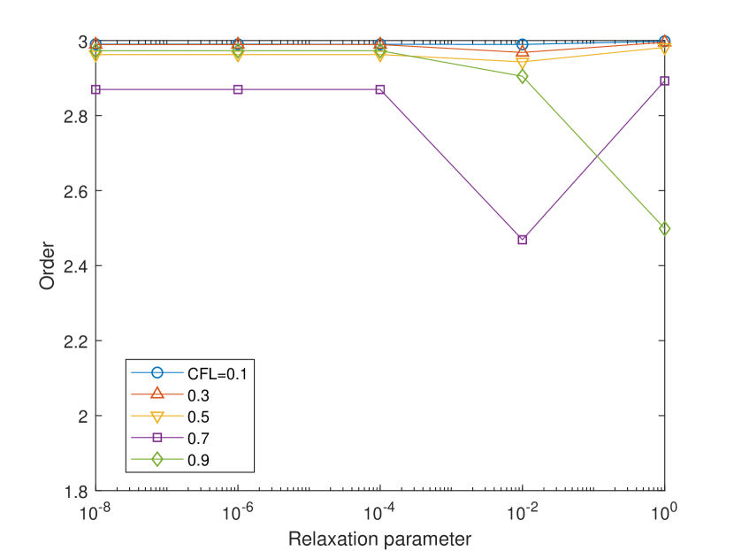
(e) BDF3, Q-CWENO23

Figure 9. Accuracy tests for 1D Broadwell model. Initial data is associated to (5.4). $x$-axis is for the relaxation parameter $\kappa$ and $y$-axis is for order of accuracy based on $N_{x}=160,320,640$.

5.3. Shock tests

We consider the following two cases in [4]:

(5.5) $$\begin{split}\text{Case 1.}\,(\rho,\,m,\,z)=&\begin{cases}(2,1,1)\quad x<0.2\\ (1,0.13962,1)\quad x>0.2\\ \end{cases},\,x\in[-1,1],\,T^{f}=0.25,\,\kappa=1,\\ \text{Case 2.}\,(\rho,\,m,\,z)=&\begin{cases}(1,0,1)\quad x<0.5\\ (0.2,0,1)\quad x>0.5\\ \end{cases},\,x\in[0,1],\,T^{f}=0.25,\,\kappa=10^{-8}.\end{split}$$

For each case, we take $N_{x}=200$. In Fig. 10 we observe that the proposed schemes allows large CFL$>1$ with the choice of $\kappa=1$. In case of $\kappa=10^{-8}$, some oscillations appear near the discontinuity for CFL$>0.8$. For CFL$\leq 0.8$, we obtain solutions which reproduce the numerical results in [4].

(a) DIRK2, Q-CWENO23, CFL$=0.5$

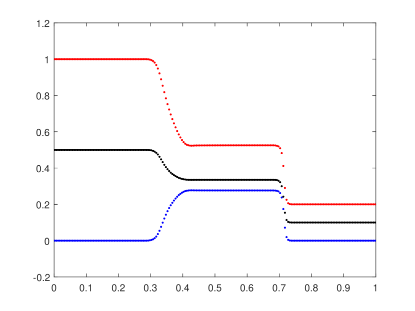
(b) DIRK2, Q-CWENO23, CFL$=0.5$

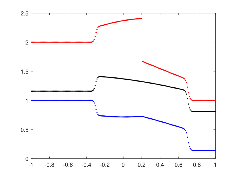
(c) DIRK2, Q-CWENO23, CFL$=0.8$

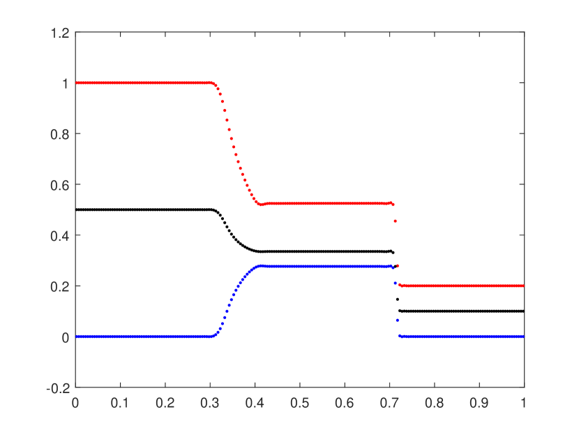
(d) DIRK2, Q-CWENO23, CFL$=0.8$

(e) DIRK2, Q-CWENO23, CFL$=1.9$

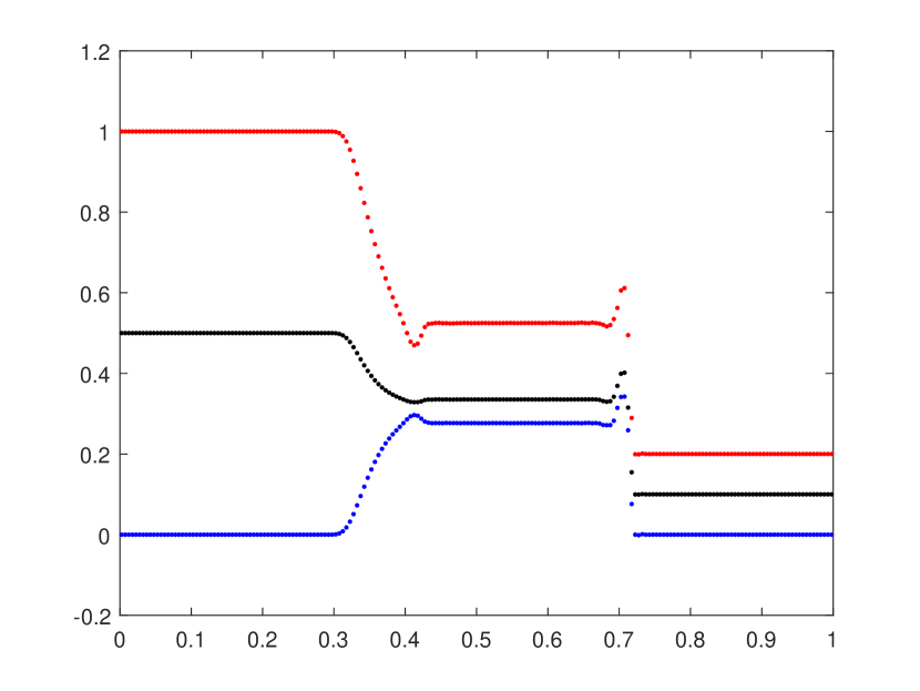
(f) DIRK2, Q-CWENO23, CFL$=1.9$

Figure 10. Shock tests for 1D Broadwell model. Macroscopic variables $\rho$ (red), $m$ (blue) and $z$ (black). Left: Case 1 in (5.5), Right: Case 2 in (5.5).

5.4. 2D simplified Xin-Jin model

For 2D tests, we here consider the DIRK2 based method.

5.4.1. Accuracy test

Here, we use well-prepared initial data:

(5.6) $$u_{0}(x,y)=0.8\sin^{2}(\pi x)\sin^{2}(\pi y),\quad v_{0}(x,y)=\frac{u_{0}^{2}(x,y)}{2}+\kappa\left(u_{0}^{2}(x,y)-1\right)(\partial_{x}{u_{0}}(x,y)+\partial_{y}{u_{0}}(x,y)).$$

The computation is performed in $(x,y)\in[0,1]^{2}$ with the periodic boundary condition with $N_{x}=N_{y}$. In this problem, the breaking time is $\displaystyle T_{b}=\frac{1}{0.6\pi\sqrt{3}}\approx 0.3063$, we take a final time as $\displaystyle T^{f}=0.15$. Since $|u_{0}|<1$, the subcharacteristic condition is satisfied. We restrict the ratio to satisfy $\frac{\Delta t}{\Delta x}\leq 1$. In Fig. 11, we confirm that SL schemes based on DIRK2 and BDF2 attains desired accuracy between 2 and 3 for all ranges of the relaxation parameter $\kappa$.

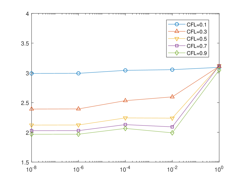
(a) DIRK2 - Q-CWENO23

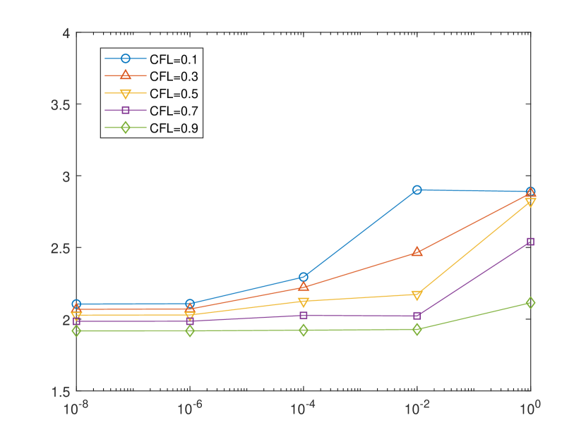
(b) BDF2 - Q-CWENO23

Figure 11. Accuracy tests for 2D Xin-Jin model. Initial data is associated to (5.6). $x$-axis is for the relaxation parameter $\kappa$ and $y$-axis is for order of accuracy based on $N_{x}^{2}=N_{y}^{2}=160^{2},320^{2},640^{2}$.

5.4.2. Shock tests

Now, we move on to 2D shock tests for (4.6).
$\bullet$ Smooth initial data. Here, we solve the relaxation system (4.6) to capture the profile of the shock in Burgers equation. For this, we consider the following initial data:

(5.7) $$u_{0}(x,y)=0.8\sin^{2}(\pi x)\sin^{2}(\pi y),\quad v_{0}(x,y)=\frac{u_{0}^{2}(x,y)}{2}.$$

on the periodic domain $(x,y)\in[0,1]^{2}$ with grid points $N_{x}=400$ and mesh ratio $\frac{\Delta t}{\Delta x}=\frac{\Delta t}{\Delta y}=0.2$. In Fig. 12, results are reported for $t=1,2,3$. Here, we only present result using 2D SL methods based on DIRK2 and Q-CWENO23.

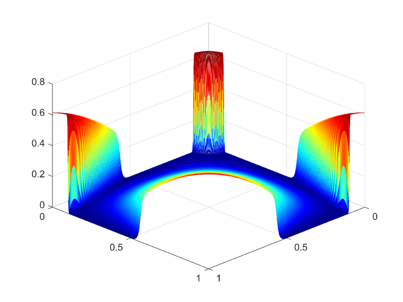
(a) $t=1$

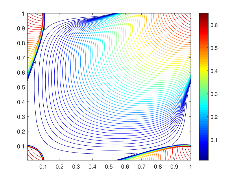
(b) $t=1$

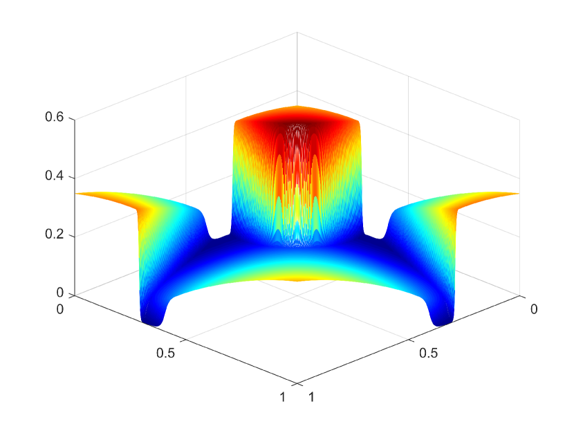
(c) $t=2$

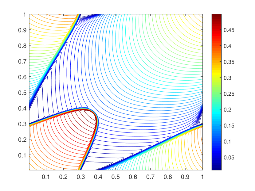
(d) $t=2$

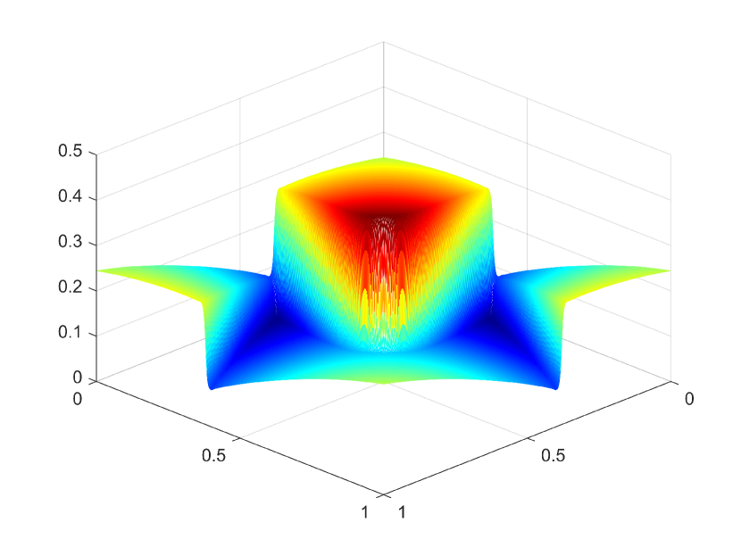
(e) $t=3$

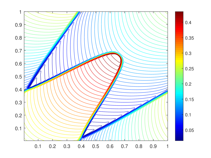
(f) $t=3$

Figure 12. Shock test for 2D Xin-Jin model. Initial data is associated to (5.7). Numerical solutions are obtained by DIRK2 based SL scheme for $\kappa=10^{-4}$. Mesh plot (left) and contour plot (right) of the solution $u$ at various times $t=1,2,3$.

$\bullet$ Discontinuous initial data. This test has been solved by solving a viscous Burgers equation in [15]. Here, we instead solve the relaxation system (4.6) to capture the correct shock position of Burgers equation. Initial data is given by

(5.8) $$u_{0}(x)=\begin{cases}-0.5,\quad x\leq 0,y\leq 0\\ \,0.25,\quad x\leq 0,y>0\\ \,0.25,\quad x>0,y\leq 0\\ \,0.5,\quad x>0,y>0\end{cases},\quad v_{0}(x,y)=\frac{u_{0}^{2}(x,y)}{2}$$

with freeflow boundary condition $(x,y)\in[-1,1].^{2}$ with grid points $N_{x}=400$ and mesh ration $\frac{\Delta t}{\Delta x}=\frac{\Delta t}{\Delta y}=0.2$. In Fig. 13, we plot the results for $t=1,2,3$. We only present result using 2D SL methods based on DIRK2 and Q-CWENO23.

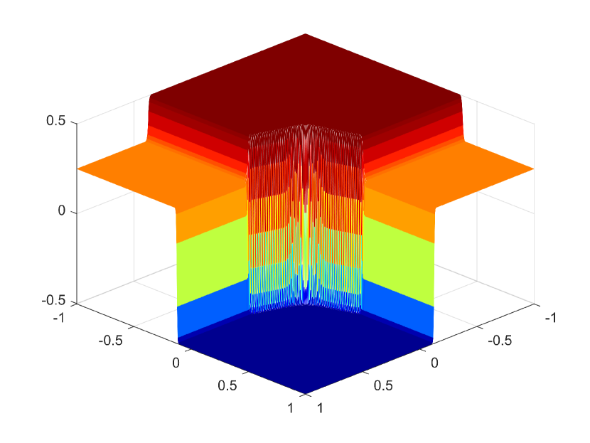
(a) $t=1$

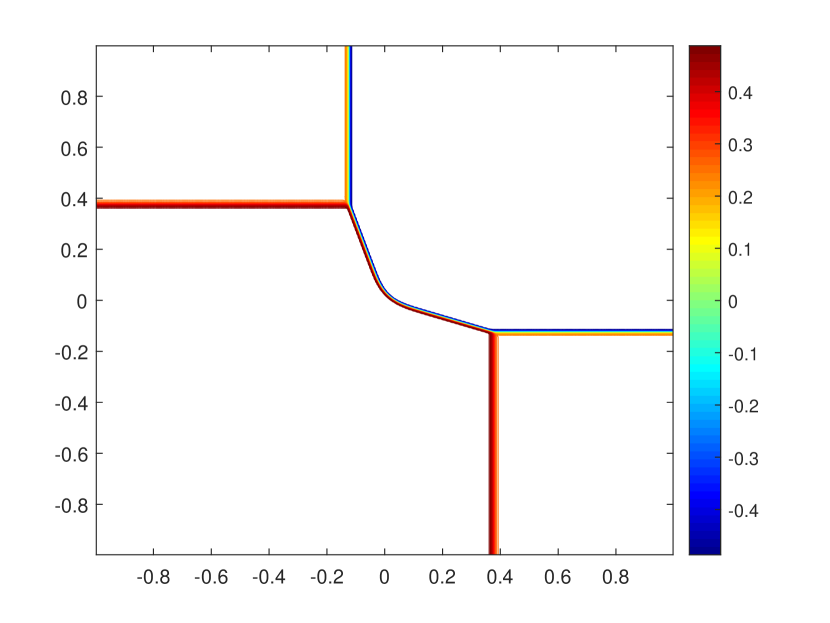
(b) $t=1$

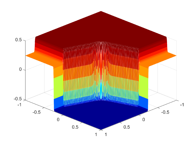
(c) $t=2$

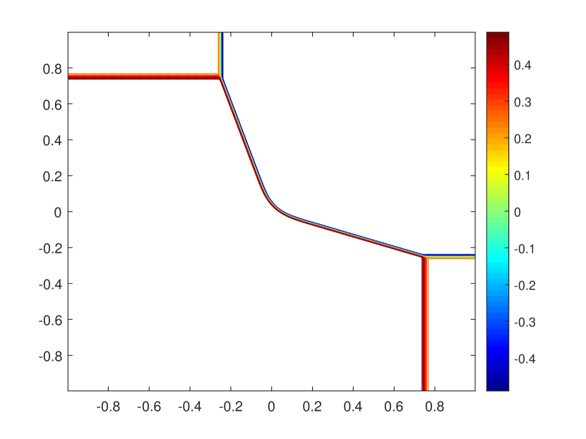
(d) $t=2$

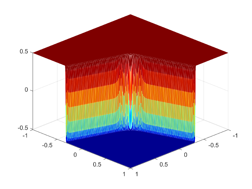
(e) $t=3$

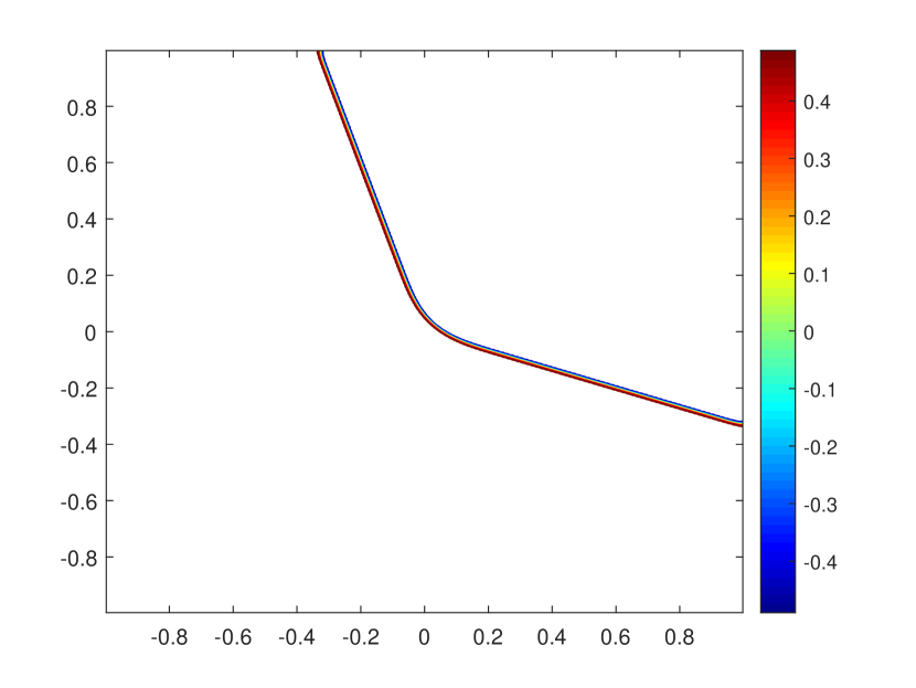
(f) $t=3$

Figure 13. Shock test for 2D Xin-Jin model. Initial data is associated to (5.8). Numerical solutions are obtained by DIRK2 based SL scheme for $\kappa=10^{-4}$. Mesh plot (left) and contour plot (right) of the solution $u$ at various times $t=1,2,3$.

6. Conclusions

We propose a simple technique to restore conservation in semi-Lagrangian schemes when non-linear reconstructions are adopted to avoid spurious oscillation or to preserve the positivity of the solution. The reconstruction is obtained by taking the sliding average of a basic non-oscillatory (positive-preserving) cell-average to point-wise reconstruction $R$, thus it inherits the non-oscillatory (positivity-preserving) property of $R$. A detailed analysis is performed of the proposed reconstruction, proving its accuracy and conservation properties, and its consistency with Lagrange interpolation in the case of linear basic reconstruction. Two dimensional extension is also considered and analyzed. The technique is then tested on the Xin-Jin relaxation system in one and two space dimensions, and on the 1D Broadwell model. Applications to BGK model and Vlasov-Poisson system will be presented in the second part of the paper.

Appendix A Proof of Proposition 2.1

Proof.

We first write (2.7) as

(A.1) $$\begin{split}Q_{i+\theta}&=\sum_{\ell=\text{even}}^{k}(\Delta x)^{\ell}\left(\alpha_{\ell}(\theta)R_{i}^{(\ell)}+\left(\frac{1}{(\ell+1)!}\left(\frac{1}{2}\right)^{\ell}-\alpha_{\ell}(\theta)\right)R_{i+1}^{(\ell)}\right)+\sum_{\ell=\text{odd}}^{k}(\Delta x)^{\ell}\alpha_{\ell}(\theta)\left(R_{i}^{(\ell)}-R_{i+1}^{(\ell)}\right).\end{split}$$

This, together with the assumption (2.12), gives

$$Q_{i+\theta} =\sum_{\ell=\text{even}}^{k}(\Delta x)^{\ell}\left(\alpha_{\ell}(\theta)u_{i}^{(\ell)}+\left(\frac{1}{(\ell+1)!}\left(\frac{1}{2}\right)^{\ell}-\alpha_{\ell}(\theta)\right)u_{i+1}^{(\ell)}\right)$$

$$\quad+\sum_{\ell=\text{odd}}^{k}(\Delta x)^{\ell}\alpha_{\ell}(\theta)\left(u_{i}^{(\ell)}-u_{i+1}^{(\ell)}\right)+(\Delta x)^{k+2}$$

$$=\sum_{\ell=0}^{k}(\Delta x)^{\ell}\left(\alpha_{\ell}(\theta)u_{i}^{(\ell)}+\beta_{\ell}(\theta)u_{i+1}^{(\ell)}\right)+(\Delta x)^{k+2}.$$

Using Taylor’s expansion $u_{i+1}^{(\ell)}=u_{i}^{(\ell)}+u_{i}^{(\ell+1)}\Delta x+\frac{1}{2}u_{i}^{(\ell+2)}(\Delta x)^{2}+\frac{1}{6}u_{i}^{(\ell+3)}(\Delta x)^{3}+\cdots$, we obtain

$$Q_{i+\theta} =\sum_{\ell=0}^{k}(\Delta x)^{\ell}\left(\alpha_{\ell}(\theta)u_{i}^{(\ell)}+\beta_{\ell}(\theta)\sum_{m=0}^{k+1-\ell}\frac{u_{i}^{(\ell+m)}}{m!}(\Delta x)^{m}\right)+\mathcal{O}\left((\Delta x)^{k+2}\right)$$

$$=\sum_{\ell=0}^{k}(\Delta x)^{\ell}\alpha_{\ell}(\theta)u_{i}^{(\ell)}+\sum_{\ell=0}^{k}\sum_{m=0}^{k-\ell}(\Delta x)^{\ell+m}\beta_{\ell}(\theta)\frac{u_{i}^{(\ell+m)}}{m!}+\sum_{\ell=0}^{k}(\Delta x)^{k+1}\beta_{\ell}(\theta)\frac{u_{i}^{(k+1)}}{(k+1-\ell)!}+\mathcal{O}\left((\Delta x)^{k+2}\right)$$

$$=:\sum_{\ell=0}^{k}(\Delta x)^{\ell}\lambda_{\ell}(\theta)u_{i}^{(\ell)}+\sum_{\ell=0}^{k}(\Delta x)^{k+1}\beta_{\ell}(\theta)\frac{u_{i}^{(k+1)}}{(k+1-\ell)!}+\mathcal{O}\left((\Delta x)^{k+2}\right),$$

where $\displaystyle\lambda_{\ell}(\theta)=\alpha_{\ell}(\theta)+\sum_{m=0}^{\ell}\beta_{m}(\theta)\frac{1}{(\ell-m)!}$. Note that

$$\sum_{\ell=0}^{k}\beta_{\ell}(\theta)\frac{1}{(k+1-\ell)!} =\alpha_{k+1}(\theta)+\sum_{m=0}^{k+1}\beta_{m}(\theta)\frac{1}{(k+1-m)!}=\lambda_{k+1}(\theta).$$

The first equality follows from $\alpha_{k+1}(\theta)+\beta_{k+1}(\theta)=0$, which holds due to (2.9) for an even integer $k$. To sum up,

$$Q_{i+\theta} =\sum_{\ell=0}^{k+1}(\Delta x)^{\ell}\lambda_{\ell}(\theta)u_{i}^{(\ell)}+\mathcal{O}\left((\Delta x)^{k+2}\right),$$

and this can be written explicitly as follows:

$$Q_{i+\theta} =u_{i}^{(0)}+\theta u_{i}^{(1)}\Delta x+\left(\frac{\theta^{2}}{2}+\frac{1}{24}\right)u_{i}^{(2)}(\Delta x)^{2}+\left(\frac{\theta^{3}}{6}+\frac{\theta}{24}\right)u_{i}^{(3)}(\Delta x)^{3}$$

$$\quad+\left(\frac{\theta^{4}}{24}+\frac{\theta^{2}}{48}+\frac{1}{1920}\right)u_{i}^{(4)}(\Delta x)^{4}+\left(\frac{\theta^{5}}{120}+\frac{\theta^{3}}{144}+\frac{\theta}{1920}\right)u_{i}^{(5)}(\Delta x)^{5}$$

$$+\left(\frac{\theta^{6}}{720}+\frac{\theta^{4}}{576}+\frac{\theta^{2}}{3840}+\frac{1}{322560}\right)u_{i}^{(6)}(\Delta x)^{6}+\cdots+\mathcal{O}\left((\Delta x)^{k+2}\right)$$

$$=\sum_{\ell=0}^{k+1}\frac{\theta^{\ell}}{\ell!}u_{i}^{(\ell)}(\Delta x)^{\ell}+\frac{(\Delta x)^{2}}{24}\sum_{\ell=0}^{k-1}\frac{\theta^{\ell}}{\ell!}u_{i}^{(\ell+2)}(\Delta x)^{\ell}+\frac{(\Delta x)^{4}}{1920}\sum_{\ell=0}^{k-3}\frac{\theta^{\ell}}{\ell!}u_{i}^{(\ell+4)}(\Delta x)^{\ell}$$

$$\quad+\frac{(\Delta x)^{6}}{322560}\sum_{\ell=0}^{k-5}\frac{\theta^{\ell}}{\ell!}u_{i}^{(\ell+4)}(\Delta x)^{\ell}+\cdots+\mathcal{O}\left((\Delta x)^{k+2}\right).$$

Consequently, we can derive

$$Q_{i+\theta} =u(x_{i+\theta})+\frac{(\Delta x)^{2}}{24}u^{(2)}(x_{i+\theta})+\frac{(\Delta x)^{4}}{1920}u^{(4)}(x_{i+\theta})+\cdots+\mathcal{O}\left((\Delta x)^{k+2}\right)$$

$$=\sum_{\ell=\text{even}}^{k}\left(\Delta x\right)^{\ell}u^{(\ell)}(x_{i+\theta})\frac{1}{(\ell+1)!}\left(\frac{1}{2}\right)^{\ell}+\mathcal{O}\left((\Delta x)^{k+2}\right)$$

$$=\bar{u}(x_{i+\theta})+\mathcal{O}\left((\Delta x)^{k+2}\right).$$

∎

Appendix B Proof of Remark 2.1

Consider any polynomial reconstruction $R_{i}(x),R_{i+1}(x)\in\mathbb{P}^{k}$ of the form (2.4) such that

$$u^{(\ell)}(x_{i})-R_{i}^{(\ell)}=\mathcal{O}\left((\Delta x)^{k+1-\ell}\right),\quad u^{(\ell)}(x_{i+1})-R_{i+1}^{(\ell)}=\mathcal{O}\left((\Delta x)^{k+1-\ell}\right).$$

From the assumption that $R_{i}^{(\ell)}$ is represented by Lipschitz functions $F_{\ell}$ of $\{\bar{u}_{i-r},\cdots,\bar{u}_{i+s}\}$, we can write it as

$$R_{i}^{(\ell)}=u^{(\ell)}(x_{i})+F_{\ell}\left(\bar{u}_{i-r},\cdots,\bar{u}_{i+s}\right)-u^{(\ell)}(x_{i}),$$

where $F_{\ell}\left(\bar{u}_{i-r},\cdots,\bar{u}_{i+s}\right)-u^{(\ell)}(x_{i})=\mathcal{O}\left((\Delta x)^{k+1-\ell}\right).$ Also, in (2.13), one can see that the function $p_{i}^{(\ell)}\in\mathbb{P}^{k-\ell}$ is written with a Lipschitz function $G_{\ell}$ of $\{\bar{u}_{i-r},\cdots,\bar{u}_{i+s}\}$ such that

$$p_{i}^{(\ell)}=u^{(\ell)}(x_{i})+G_{\ell}\left(\bar{u}_{i-r},\cdots,\bar{u}_{i+s}\right)-u^{(\ell)}(x_{i}),\quad G_{\ell}\left(\bar{u}_{i-r},\cdots,\bar{u}_{i+s}\right)-u^{(\ell)}(x_{i}) =\mathcal{O}\left((\Delta x)^{k+1-\ell}\right).$$

Now, let us define $H_{\ell}\left(\{\bar{u}_{i-r},\cdots,\bar{u}_{i+s}\}\right)$ by

$$H_{\ell}\left(\bar{u}_{i-r},\cdots,\bar{u}_{i+s}\right):=G_{\ell}\left(\bar{u}_{i-r},\cdots,\bar{u}_{i+s}\right)-F_{\ell}\left(\bar{u}_{i-r},\cdots,\bar{u}_{i+s}\right),$$

then it is Lipschitz continuous w.r.t. $\{\bar{u}_{i-r},\cdots,\bar{u}_{i+s}\}$ and $H^{\ell}\left(\bar{u}_{i-r},\cdots,\bar{u}_{i+s}\right)=\mathcal{O}\left((\Delta x)^{k+1-\ell}\right)$. Consequently,

$$u^{(\ell)}(x_{i})-R_{i}^{(\ell)}-\left(u^{(\ell)}(x_{i+1})-R_{i+1}^{(\ell)}\right)$$

$$\quad=\left\{u^{(\ell)}(x_{i})-p_{i}^{(\ell)}-\left(u^{(\ell)}(x_{i+1})-p_{i+1}^{(\ell)}\right)\right\}+\left(p_{i}^{(\ell)}-R_{i}^{(\ell)}\right)-\left(p_{i+1}^{(\ell)}-R_{i+1}^{(\ell)}\right)$$

$$\quad=\mathcal{O}\left((\Delta x)^{k+2-\ell}\right)+H_{\ell}\left(\{\bar{u}_{i-r},\cdots,\bar{u}_{i+s}\}\right)-H_{\ell}\left(\{\bar{u}_{i+1-r},\cdots,\bar{u}_{i+1+s}\}\right)$$

$$\quad=\mathcal{O}\left((\Delta x)^{k+2-\ell}\right).$$

Appendix C Proof of Proposition 2.2

Proof.

The proof is divided into three steps

Step 1, Reconstruction of $R_{i}(x)$: This polynomial reconstruction is also introduced in [35]. Given cell average values $\{\bar{u}_{i}\}$, we first consider a primitive function $U(x):=\int_{-\infty}^{x}u(x)dx$ and compute its cell boundary values as

$$U(x_{i+j-\frac{1}{2}})=\int_{-\infty}^{x_{i+j-\frac{1}{2}}}u(x)\,dx=\sum_{m=-\infty}^{i+j-1}\bar{u}_{m}\Delta x,\quad-r\leq j\leq r+1.$$

Then, look for a polynomial $P_{i}(x)$ such that

$$P_{i}(x_{i+j-\frac{1}{2}})=U(x_{i+j-\frac{1}{2}}),\quad-r\leq j\leq r+1.$$

By differentiating $P_{i}(x)$, we obtain the basic reconstruction $R_{i}(x)$ which satisfies

$$P_{i}^{\prime}(x)=R_{i}(x)=u(x)+\mathcal{O}\left((\Delta x)^{k+1}\right)$$

and the condition (2.14). The resulting form of $R_{i}(x)$ is given by

$$\displaystyle R_{i}(x)=\sum_{m=1}^{k+1}\sum_{j=0}^{m-1}\bar{u}_{i-r+j}\Delta x\left\{\frac{\sum_{\ell=0,\ell\neq m}^{k+1}\prod_{q=0,q\neq m,\ell}^{k+1}\left(x-x_{i-r+\ell-\frac{1}{2}}\right)}{\prod_{\ell=0,\ell\neq m}^{k+1}\left(x_{i-r+m-\frac{1}{2}}-x_{i-r+\ell-\frac{1}{2}}\right)}\right\}.$$

Step 2, Reconstruction of $Q_{i+\theta}$: To reconstruct $Q_{i+\theta}$, we first compute the cell average value of $R_{i}(x)$ on $[x_{i-\frac{1}{2}+\theta},x_{i+\frac{1}{2}})$:

(C.1) $$\frac{1}{\Delta x} \int_{x_{i-\frac{1}{2}+\theta}}^{x_{i+\frac{1}{2}}}R_{i}(x)\,dx=\sum_{m=1}^{k+1}\sum_{j=0}^{m-1}\bar{u}_{i-r+j}\left\{\frac{\prod_{\ell=0,\ell\neq m}^{k+1}(r-\ell+1)-\prod_{\ell=0,\ell\neq m}^{k+1}(\theta+r-\ell)}{\prod_{\ell=0,\ell\neq m}^{k+1}\left(m-\ell\right)}\right\},$$

which directly come from

$$\int_{x_{i-\frac{1}{2}+\theta}}^{x_{i+\frac{1}{2}}} \left(\sum_{\ell=0,\ell\neq m}^{k+1}\prod_{q=0,q\neq m,\ell}^{k+1}\left(x-x_{i-r+\ell-\frac{1}{2}}\right)\right)\,dx=\prod_{\ell=0,\ell\neq m}^{k+1}x_{r-\ell+1}-\prod_{\ell=0,\ell\neq m}^{k+1}x_{\theta+r-\ell}.$$

Similarly, we compute the cell average of $R_{i+1}(x)$ on $[x_{i+\frac{1}{2}},x_{i+\frac{1}{2}+\theta})$:

(C.2) $$\frac{1}{\Delta x} \int_{x_{i+\frac{1}{2}}}^{x_{i+\frac{1}{2}+\theta}}R_{i+1}(x)\,dx=\sum_{m=1}^{k+1}\sum_{j=1}^{m}\bar{u}_{i-r+j}\left\{\frac{\prod_{\ell=0,\ell\neq m}^{k+1}(\theta+r-\ell)-\prod_{\ell=0,\ell\neq m}^{k+1}(r-\ell)}{\prod_{\ell=0,\ell\neq m}^{k+1}\left(m-\ell\right)}\right\}.$$

Now, we insert (C.1) and (C.2) into the identity for $Q_{i+\theta}$ in (2.3):

$$\begin{split}Q_{i+\theta}&=\frac{1}{\Delta x}\int_{x_{i-\frac{1}{2}+\theta}}^{x_{i+\frac{1}{2}}}R_{i}(x)\,dx+\frac{1}{\Delta x}\int_{x_{i+\frac{1}{2}}}^{x_{i+\frac{1}{2}+\theta}}R_{i+1}(x)\,dx,\end{split}$$

and decompose this into four parts:

$$\begin{split}Q_{i+\theta}&=\sum_{j=0}\sum_{m=j+1}^{k+1}\bar{u}_{i-r+j}\left\{\frac{\prod_{\ell=0,\ell\neq m}^{k+1}(r-\ell+1)-\prod_{\ell=0,\ell\neq m}^{k+1}(\theta+r-\ell)}{\prod_{\ell=0,\ell\neq m}^{k+1}\left(m-\ell\right)}\right\}\cr&\quad+\sum_{j=k+1}\sum_{m=j}^{k+1}\bar{u}_{i-r+j}\left\{\frac{\prod_{\ell=0,\ell\neq m}^{k+1}(\theta+r-\ell)-\prod_{\ell=0,\ell\neq m}^{k+1}(r-\ell)}{\prod_{\ell=0,\ell\neq m}^{k+1}\left(m-\ell\right)}\right\}\cr&\quad+\sum_{j=1}^{k}\sum_{m=j}\bar{u}_{i-r+j}\left\{\frac{\prod_{\ell=0,\ell\neq m}^{k+1}(\theta+r-\ell)-\prod_{\ell=0,\ell\neq m}^{k+1}(r-\ell)}{\prod_{\ell=0,\ell\neq m}^{k+1}\left(m-\ell\right)}\right\}\cr&\quad+\sum_{j=1}^{k}\sum_{m=j+1}^{k+1}\bar{u}_{i-r+j}\left\{\frac{\prod_{\ell=0,\ell\neq m}^{k+1}(r-\ell+1)-\prod_{\ell=0,\ell\neq m}^{k+1}(r-\ell)}{\prod_{\ell=0,\ell\neq m}^{k+1}\left(m-\ell\right)}\right\}\cr&=:I_{1}+I_{2}+I_{3}+I_{4}.\end{split}$$

With the identity $\displaystyle\sum_{m=0}^{k+1}\frac{\prod_{\ell=0,\ell\neq m}^{k+1}\left(\theta+r-\ell\right)}{\prod_{\ell=0,\ell\neq m}^{k+1}\left(m-\ell\right)}=1$, we can simplify $I_{1}$ as

(C.3) $$\begin{split}I_{1}&=\bar{u}_{i-r}\sum_{m=1}^{k+1}\left\{\frac{\prod_{\ell=0,\ell\neq m}^{k+1}(r-\ell+1)-\prod_{\ell=0,\ell\neq m}^{k+1}(\theta+r-\ell)}{\prod_{\ell=0,\ell\neq m}^{k+1}\left(m-\ell\right)}\right\}\cr&=\bar{u}_{i-r}\left(\sum_{m=r+1}\frac{\prod_{\ell=0,\ell\neq m}^{k+1}(r-\ell+1)}{\prod_{\ell=0,\ell\neq m}^{k+1}\left(m-\ell\right)}-\sum_{m=1}^{k+1}\frac{\prod_{\ell=0,\ell\neq m}^{k+1}(\theta+r-\ell)}{\prod_{\ell=0,\ell\neq m}^{k+1}\left(m-\ell\right)}\right)\cr&=\bar{u}_{i-r}\left(1-\sum_{m=1}^{k+1}\frac{\prod_{\ell=0,\ell\neq m}^{k+1}(\theta+r-\ell)}{\prod_{\ell=0,\ell\neq m}^{k+1}\left(m-\ell\right)}\right)\cr&=\bar{u}_{i-r}\frac{\prod_{\ell=1}^{k+1}(\theta+r-\ell)}{\prod_{\ell=1}^{k+1}\left(-\ell\right)}.\end{split}$$

The $I_{2}$ and $I_{3}$ terms are calculated as

(C.4) $$\begin{split}I_{2}&=\bar{u}_{i+r+1}\left\{\frac{\prod_{\ell=0}^{k}(\theta+r-\ell)-\prod_{\ell=0}^{k}(r-\ell)}{\prod_{\ell=0}^{k}\left(k+1-\ell\right)}\right\}=\bar{u}_{i+r+1}\frac{\prod_{\ell=0}^{k}\theta+r-\ell}{\prod_{\ell=0}^{k}k+1-\ell}\cr I_{3}&=\sum_{j=1}^{k}\bar{u}_{i-r+j}\left\{\frac{\prod_{\ell=0,\ell\neq j}^{k+1}(\theta+r-\ell)-\prod_{\ell=0,\ell\neq j}^{k+1}(r-\ell)}{\prod_{\ell=0,\ell\neq j}^{k+1}\left(j-\ell\right)}\right\}\cr&=\bar{u}_{i}\left(\frac{\prod_{\ell=0,\ell\neq r}^{k+1}(\theta+r-\ell)}{\prod_{\ell=0,\ell\neq r}^{k+1}\left(r-\ell\right)}-1\right)+\sum_{j=1,j\neq r}^{k}\bar{u}_{i-r+j}\left\{\frac{\prod_{\ell=0,\ell\neq j}^{k+1}\theta+r-\ell}{\prod_{\ell=0,\ell\neq j}^{k+1}j-\ell}\right\}.\end{split}$$

A direct computation leads to $I_{4}=\bar{u}_{i}$. This, combined with (C.3), (C.4), gives

(C.5) $$Q_{i+\theta} =\sum_{j=0}^{k+1}\bar{u}_{i-r+j}\prod_{\ell=0,\ell\neq j}^{k+1}\frac{\theta+r-\ell}{j-\ell}.$$

Step 3, Comparison of $Q_{i+\theta}$ and $L(x_{i+\theta})$: For the comparison, we consider a Lagrange polynomial $L(x)$ which satisfies $L(x_{i-r+j})=\bar{u}_{i-r+j}$ for $0\leq j\leq k+1$:

$$L(x)=\sum_{j=0}^{k+1}\bar{u}_{i-r+j}\prod_{\ell=0,\ell\neq j}^{k+1}\frac{x-x_{i-r+\ell}}{x_{i-r+j}-x_{i-r+\ell}}.$$

Inserting $x=x_{i+\theta}$ into $L(x)$, we obtain $L(x_{i+\theta})=Q_{i+\theta}$. This completes the proof. ∎

Appendix D Proof that the condition (2.12) in Proposition 2.1 is satisfied by both CWENO23 and CWENO23Z.

Here, we check if the condition (2.12) is satisfied by (2.19). For this, we assume that $u$ is smooth enough so that $\omega_{C}^{i}=\frac{1}{2}+e_{C}^{i}$ for $e_{C}^{i}=O((\Delta x)^{2})$. We refer to [26] for the assumption. Then, we have

(D.1) $$\begin{split}R_{i}^{(0)}&=\bar{u}_{i}-\frac{1}{12}\bigg{(}C_{C}+e_{C}^{i}\bigg{)}\left(\bar{u}_{i+1}-2\bar{u}_{i}+\bar{u}_{i-1}\right)\cr&=\bar{u}_{i}-\frac{1}{12}\bigg{(}\frac{1}{2}+\mathcal{O}((\Delta x)^{2})\bigg{)}\left((\Delta x)^{2}\bar{u}^{\prime\prime}_{i}+\mathcal{O}((\Delta x)^{4})\right)\cr&=\bar{u}_{i}-\frac{1}{24}\left((\Delta x)^{2}\bar{u}^{\prime\prime}_{i}\right)+\mathcal{O}((\Delta x)^{4})\cr&=u_{i}+\mathcal{O}((\Delta x)^{4}).\end{split}$$

Similarly, we write $\omega_{L}^{i}=\frac{1}{4}+e_{L}^{i}$ and $\omega_{R}^{i}=\frac{1}{4}+e_{R}^{i}$ with $e_{L}^{i},e_{R}^{i}=\mathcal{O}((\Delta x)^{2})$. Then,

$$R_{i}^{(1)} =\omega_{L}^{i}\frac{\bar{u}_{i}-\bar{u}_{i-1}}{\Delta x}+\omega_{R}^{i}\frac{\bar{u}_{i+1}-\bar{u}_{i}}{\Delta x}+\omega_{C}^{i}\frac{\bar{u}_{i+1}-\bar{u}_{i-1}}{2\Delta x}$$

$$=\bigg{(}\frac{1}{4}+e_{L}^{i}\bigg{)}\bigg{[}\bar{u}^{\prime}_{i}-\frac{\Delta x}{2}\bar{u}^{\prime\prime}_{i}+\frac{(\Delta x)^{2}}{6}\bar{u}^{\prime\prime\prime}_{i}\bigg{]}+\bigg{(}\frac{1}{4}+e_{R}^{i}\bigg{)}\bigg{[}\bar{u}^{\prime}_{i}+\frac{\Delta x}{2}\bar{u}^{\prime\prime}_{i}+\frac{(\Delta x)^{2}}{6}\bar{u}^{\prime\prime\prime}_{i}\bigg{]}$$

$$\quad+\bigg{(}\frac{1}{2}+e_{C}^{i}\bigg{)}\bigg{[}\bar{u}^{\prime}_{i}+\frac{1}{6}(\Delta x)^{2}\bar{u}^{\prime\prime\prime}_{i}\bigg{]}+\mathcal{O}((\Delta x)^{3})$$

$$=\bar{u}^{\prime}_{i}+\frac{(\Delta x)^{2}}{6}\bar{u}^{\prime\prime\prime}_{i}+\mathcal{O}((\Delta x)^{3}).$$

In the last equality, we used $\sum_{k}\omega_{k}^{i}=1$. Hence, we can obtain

(D.2) $$\begin{split}R_{i}^{(1)}-R_{i+1}^{(1)}&=\bar{u}^{\prime}_{i}-\bar{u}^{\prime}_{i+1}+\frac{(\Delta x)^{2}}{6}(\bar{u}^{\prime\prime\prime}_{i}-\bar{u}^{\prime\prime\prime}_{i+1})+\mathcal{O}((\Delta x)^{3})\cr&=\bar{u}^{\prime}_{i}-\bar{u}^{\prime}_{i+1}-\frac{(\Delta x)^{2}}{24}(\bar{u}^{\prime\prime\prime}_{i}-\bar{u}^{\prime\prime\prime}_{i+1})+\mathcal{O}((\Delta x)^{3})\cr&=\bigg{(}\bar{u}^{\prime}_{i}-\frac{(\Delta x)^{2}}{24}\bar{u}^{\prime\prime\prime}_{i}\bigg{)}-\bigg{(}\bar{u}^{\prime}_{i+1}-\frac{(\Delta x)^{2}}{24}\bar{u}^{\prime\prime\prime}_{i+1}\bigg{)}+\mathcal{O}((\Delta x)^{3})=u^{\prime}_{i}-u^{\prime}_{i+1}+\mathcal{O}((\Delta x)^{3}).\end{split}$$

It is straightforward to show that

(D.3) $$\begin{split}R_{i}^{(2)}=2\omega_{C}^{i}\frac{\bar{u}_{i+1}-2\bar{u}_{i}+\bar{u}_{i-1}}{(\Delta x)^{2}}&=2\bigg{(}\frac{1}{2}+e_{C}^{i}\bigg{)}\bigg{[}\frac{\bar{u}_{i+1}-2\bar{u}_{i}+\bar{u}_{i-1}}{(\Delta x)^{2}}\bigg{]}\cr&=\bigg{(}1+\mathcal{O}((\Delta x)^{2})\bigg{)}\bigg{[}\bar{u}^{\prime\prime}_{i}+\frac{(\Delta x)^{2}}{12}\bar{u}^{(4)}_{i}\bigg{]}=u^{\prime\prime}_{i}+\mathcal{O}((\Delta x))^{2}.\end{split}$$

From (D.1),(D.2) and (D.3), we confirm that (2.19) satisfies the condition (2.15) with $k=2$.

Appendix E Explicit form of $R_{i}^{(\ell)}$.

For $k=4$ in the 1D Algorithm 2.2.3, we can take CWENO35 reconstruction as a basic reconstruction $R$. We refer to [6] for details on CWENO35 reconstruction. Here we can represent it as the following explicit form of $R_{i}(x)$:

(E.1) $$R_{i}(x)=\sum_{\ell=0}^{4}\frac{R_{i}^{(\ell)}}{\ell!}(x-x_{i})^{(\ell)},$$

with

(E.2) $$\begin{split}R_{i}^{(0)}&=\omega_{C}\left(\frac{577}{480}u_{i}-\frac{29}{240}u_{i-1}+\frac{19}{960}u_{i-2}-\frac{29}{240}u_{i+1}+\frac{19}{960}u_{i+2}\right)\cr&\quad-\omega_{2}\left(\frac{u_{i-1}-26u_{i}+u_{i+1}}{24}\right)+\omega_{1}\left(\frac{23}{24}u_{i}+\frac{1}{12}u_{i-1}-\frac{1}{24}u_{i-2}\right)+\omega_{3}\left(\frac{23}{24}u_{i}+\frac{1}{12}u_{i+1}-\frac{1}{24}u_{i+2}\right)\cr R_{i}^{(1)}&=-\omega_{C}\frac{8u_{i-1}-u_{i-2}-8u_{i+1}+u_{i+2}}{12\Delta x}+\omega_{1}\frac{3u_{i}-4u_{i-1}+u_{i-2}}{2\Delta x}\cr&\quad-\omega_{3}\frac{3u_{i}-4u_{i+1}+u_{i+2}}{2\Delta x}-\omega_{2}\frac{u_{i-1}-u_{i+1}}{2\Delta x}\cr R_{i}^{(2)}&=2\bigg{(}\omega_{1}\frac{u_{i}-2u_{i-1}+u_{i-2}}{2(\Delta x)^{2}}+\omega_{2}\frac{u_{i-1}-2u_{i}+u_{i+1}}{2(\Delta x)^{2}}+\omega_{3}\frac{u_{i}-2u_{i+1}+u_{i+2}}{2(\Delta x)^{2}}\bigg{)}\cr&\quad-2\omega_{C}\bigg{(}\frac{10u_{i}-6u_{i-1}+u_{i-2}-6u_{i+1}+u_{i+2}}{4(\Delta x)^{2}}/\bigg{)}\cr R_{i}^{(3)}&=6\omega_{C}\left(\frac{u_{i-1}-u_{i+1}}{3(\Delta x)^{3}}-\frac{u_{i-2}-u_{i+2}}{6(\Delta x)^{3}}\right),\quad R_{i}^{(4)}=24\omega_{C}\left(\frac{u_{i-2}+6u_{i}+u_{i+2}}{12(\Delta x)^{4}}-\frac{u_{i-1}+u_{i+1}}{3(\Delta x)^{4}}\right).\end{split}$$

where the non-linear weights $\omega_{k}^{i}$ are computed as in (2.18). (See also [6].)

The CWENOZ5 reconstruction also can be directly obtained from [13] with the following non-linear weights:

(E.3) $$\omega_{k}^{i}=\frac{\alpha_{k}^{i}}{\sum_{\ell}\alpha_{\ell}^{i}},\quad\alpha_{k}^{i}=C_{i}\left(1+\frac{\tau}{\epsilon+{\beta}_{k}^{i}}\right)^{t},\quad k,\ell\in\{1,\,2,\,3,\,C\},$$

where $t\geq 1$ and $\tau=|\beta_{3}^{i}-\beta_{1}^{i}|$.

Appendix F Proof of Proposition 3.1

Proof.

Recall the index set in (3.5). For each index set, apply corresponding approximations in (3.4) to (3.3). Then,

(F.1) $$\begin{split}Q_{i+\theta,j+\eta}=\sum_{|\ell|=0}^{k}(\Delta)^{\ell}&\bigg{(}\alpha_{\ell_{1}}(\theta)\alpha_{\ell_{2}}(\eta)u_{i,j}^{(\ell)}+\beta_{\ell_{1}}(\theta)\alpha_{\ell_{2}}(\eta)u_{i+1,j}^{(\ell)}\cr&+\alpha_{\ell_{1}}(\theta)\beta_{\ell_{2}}(\eta)u_{i,j+1}^{(\ell)}+\beta_{\ell_{1}}(\theta)\beta_{\ell_{2}}(\eta)u_{i+1,j+1}^{(\ell)}\bigg{)}+\mathcal{O}(h^{k+2}).\end{split}$$

Now, we consider Taylor’s expansion of $u_{i+1,j}^{(\ell)},u_{i,j+1}^{(\ell)},u_{i+1,j+1}^{(\ell)}$:

$$u_{i+1,j}^{(\ell)} =\sum_{m_{1}=0}^{k-|\ell|}\frac{u_{i,j}^{(\ell_{1}+m_{1},\ell_{2})}}{m_{1}!}(\Delta x)^{m_{1}}+\frac{u_{i,j}^{(\ell_{1}+k-|\ell|+s,\ell_{2})}}{(k-|\ell|+s)!}(\Delta x)^{k-|\ell|+s}$$

$$u_{i,j+1}^{(\ell)} =\sum_{m_{2}=0}^{k-|\ell|}\frac{u_{i,j}^{(\ell_{1},\ell_{2}+m_{2})}}{m_{2}!}(\Delta y)^{m_{2}}+\frac{u_{i,j}^{(\ell_{1},\ell_{2}+k-|\ell|+s)}}{(k-|\ell|+s)!}(\Delta x)^{k-|\ell|+s}$$

$$u_{i+1,j+1}^{(\ell)} =\sum_{|m|=0}^{k-|\ell|}\frac{u_{i,j}^{(\ell+m)}}{m_{1}!m_{2}!}(\Delta)^{m}+\sum_{|m|=k-|\ell|+s}\frac{u_{i,j}^{(\ell+m)}}{m_{1}!m_{2}!}(\Delta)^{m},$$

where $m=(m_{1},m_{2})$ is an multi index. Inserting this into (F.1), we obtain

(F.2) $$\begin{split}Q_{i+\theta,j+\eta}=:\sum_{|\ell|=0}^{k}(\Delta)^{\ell}\Lambda_{\ell}(\theta,\eta)u_{i,j}^{(\ell)}+\Gamma(\theta,\eta)+\mathcal{O}\left(h^{k+2}\right),\end{split}$$

where $\Lambda_{\ell}(\theta,\eta)$ and $\Gamma(\theta,\eta)$ are given by

$$\Lambda_{\ell}(\theta,\eta) =\alpha_{\ell_{1}}(\theta)\alpha_{\ell_{2}}(\eta)+\alpha_{\ell_{2}}(\eta)\sum_{m_{1}=0}^{\ell_{1}}\beta_{m_{1}}(\theta)\frac{1}{(\ell_{1}-m_{1})!}$$

$$+\alpha_{\ell_{1}}(\theta)\sum_{m_{2}=0}^{\ell_{2}}\beta_{m_{2}}(\eta)\frac{1}{(\ell_{2}-m_{2})!}+\sum_{|m|=0}^{|\ell|}\beta_{m_{1}}(\theta)\beta_{m_{2}}(\eta)\frac{1}{(\ell_{1}-m_{1})!(\ell_{2}-m_{2})!}$$

$$\Gamma(\theta,\eta) =\sum_{|\ell|=0}^{k}\beta_{\ell_{1}}(\theta)\alpha_{\ell_{2}}(\eta)\frac{u_{i,j}^{(\ell_{1}+k-|\ell|+s,\ell_{2})}}{(k-|\ell|+s)!}(\Delta x)^{k-|\ell|+s}(\Delta)^{\ell}$$

$$\quad+\sum_{|\ell|=0}^{k}\alpha_{\ell_{1}}(\theta)\beta_{\ell_{2}}(\eta)\frac{u_{i,j}^{(\ell_{1},\ell_{2}+k-|\ell|+s)}}{(k-|\ell|+s)!}(\Delta y)^{k-|\ell|+s}(\Delta)^{\ell}$$

$$\quad+\sum_{|\ell|=0}^{k}\beta_{\ell_{1}}(\theta)\beta_{\ell_{2}}(\eta)\sum_{|m|=k-|\ell|+s}\frac{u_{i,j}^{(\ell+m)}}{m_{1}!m_{2}!}(\Delta)^{m+\ell}.$$

Now, we add $0$ to $\Gamma(\theta,\eta)$ using the following identity:

(F.3) $$\begin{split}0&=\sum_{|\ell|=k+1}\left(\alpha_{\ell_{1}}(\theta)+\beta_{\ell_{1}}(\theta)\right)\left(\alpha_{\ell_{2}}(\eta)+\beta_{\ell_{2}}(\eta)\right)u_{i,j}^{(\ell)}(\Delta)^{\ell}\cr&=\sum_{|\ell|=k+1}\alpha_{\ell_{1}}(\theta)\alpha_{\ell_{2}}(\eta)u_{i,j}^{(\ell)}(\Delta)^{\ell}+\sum_{|\ell|=k+1}\beta_{\ell_{1}}(\theta)\alpha_{\ell_{2}}(\eta)u_{i,j}^{(\ell)}(\Delta)^{\ell}\cr&\quad+\sum_{|\ell|=k+1}\alpha_{\ell_{1}}(\theta)\beta_{\ell_{2}}(\eta)u_{i,j}^{(\ell)}(\Delta)^{\ell}+\sum_{|\ell|=k+1}\beta_{\ell_{1}}(\theta)\beta_{\ell_{2}}(\eta)u_{i,j}^{(\ell)}(\Delta)^{\ell},\end{split}$$

then

$$\Gamma(\theta,\eta)+0 =\sum_{|\ell|=k+1}\alpha_{\ell_{1}}(\theta)\alpha_{\ell_{2}}(\eta)u_{i,j}^{(\ell)}(\Delta)^{\ell}+\sum_{|\ell|=0}^{k+1}\beta_{\ell_{1}}(\theta)\alpha_{\ell_{2}}(\eta)\frac{u_{i,j}^{(\ell_{1}+k-|\ell|+s,\ell_{2})}}{(k-|\ell|+s)!}(\Delta x)^{k-|\ell|+s}(\Delta)^{\ell}$$

$$\quad+\sum_{|\ell|=0}^{k+1}\alpha_{\ell_{1}}(\theta)\beta_{\ell_{2}}(\eta)\frac{u_{i,j}^{(\ell_{1},\ell_{2}+k-|\ell|+s)}}{(k-|\ell|+s)!}(\Delta y)^{k-|\ell|+s}(\Delta)^{\ell}$$

$$\quad+\sum_{|\ell|=0}^{k+1}\beta_{\ell_{1}}(\theta)\beta_{\ell_{2}}(\eta)\sum_{|m|=k-|\ell|+s}\frac{u_{i,j}^{(\ell+m)}}{m_{1}!m_{2}!}(\Delta)^{m+\ell}.$$

This reduces to

$$\Gamma(\theta,\eta)=\sum_{|\ell|=k+1}(\Delta)^{\ell}\Lambda_{\ell}(\theta,\eta)u_{i,j}^{(\ell)}.$$

Based on this formula, we rearrange all terms in (F.2) as follows:

$$Q_{i+\theta,j+\eta} =u_{i,j}+\theta\Delta xu^{\prime}_{i,j}+\eta\Delta yu_{i,j}^{\backprime}+\left(\frac{\theta^{2}}{2}+\frac{1}{24}\right)(\Delta x)^{2}u^{\prime\prime}_{i,j}+\left(\frac{\eta^{2}}{2}+\frac{1}{24}\right)(\Delta y)^{2}u_{i,j}^{\backprime\backprime}+\eta\theta\Delta x\Delta yu^{\prime\backprime}_{i,j}$$

$$\quad+\left(\frac{\theta^{3}}{6}+\frac{\theta}{24}\right)(\Delta x)^{3}u^{\prime\prime\prime}_{i,j}+\left(\frac{\eta\theta^{2}}{2}+\frac{\eta}{24}\right)(\Delta x)^{2}\Delta yu^{\prime\prime\backprime}_{i,j}$$

$$\quad+\left(\frac{\theta\eta^{2}}{2}+\frac{\theta}{24}\right)\Delta x(\Delta y)^{2}u^{\prime\backprime\backprime}_{i,j}+\left(\frac{\eta^{3}}{6}+\frac{\eta}{24}\right)(\Delta y)^{3}u_{i,j}^{\backprime\backprime\backprime}+\cdots+\mathcal{O}(h^{k+2})$$

$$=u_{i+\theta,j+\eta}+\frac{(\Delta x)^{2}}{24}u^{\prime\prime}_{i+\theta,j+\eta}+\frac{(\Delta y)^{2}}{24}u_{i+\theta,j+\eta}^{\backprime\backprime}+\cdots+\mathcal{O}(h^{k+2})$$

$$=\bar{u}_{i+\theta,j+\eta}+\mathcal{O}(h^{k+2}),$$

which completes the proof. ∎

Appendix G Semi-Lagrangian schemes for hyperbolic system with BDF methods

The BDF methods [20] for an ordinary system $y^{\prime}(t)=f(y)$ can be represented by

$$y^{n+1}=\sum_{k=1}^{s}a_{k}y^{n+1-s}+\beta_{s}f^{n+1}.$$

where $\alpha_{k}$ and $\beta_{s}$ are coefficients corresponding to s-order BDF methods. Here, we consider two cases $s=2,3$:

BDF2: $$\quad y^{n+1}=\frac{4}{3}y^{n}-\frac{1}{3}y^{n-1}+\frac{2}{3}f^{n+1}$$

BDF3: $$\quad y^{n+1}=\frac{18}{11}y^{n}-\frac{9}{11}y^{n-1}+\frac{2}{11}y^{n-1}+\frac{6}{11}f^{n+1}.$$

G.1. BDF methods for Xin-Jin model

Applying BDF method based SL methods to (4.10), we obtain:

(G.3) $$\begin{array}[]{l}\displaystyle f^{n+1}_{i}=\sum_{k=1}^{s}\alpha_{k}\,\tilde{f}^{n,k}+\beta_{s}\,\frac{\Delta t}{\kappa}\,K^{n+1}_{i,1}\\ \displaystyle g^{n+1}_{i}=\sum_{k=1}^{s}\alpha_{k}\,\tilde{g}^{n,k}+\beta_{s}\,\frac{\Delta t}{\kappa}\,K^{n+1}_{i,2}.\end{array}$$

Here we use the following notation:

• For $k=1,\dots,s$, the $(n+1-k)$th stage values of $f,g$ along the backward-characteristics which come from $x_{i}$ with characteristic speed $-1,1$ at time $t^{n+1}$:

  $$\tilde{f}_{i}^{n,k} \approx f(x_{i}+k\Delta t,t^{n+1-k}),\quad\tilde{g}_{i}^{n,k}\approx g(x_{i}-k\Delta t,t^{n+1-k}).$$

• Fluxes at time $t^{n+1}$:

  $$K^{n+1}_{i,1}\approx F(u_{i}^{n+1})-v_{i}^{n+1},\quad K^{n+1}_{i,2}\approx-K^{n+1}_{i,1}.$$

The algorithm can be summarized as follows:

Algorithm of $s$-order BDF methods

1. For $k=1,2,\dots,s$, interpolate $\tilde{f}_{i}^{n,k}$ and $\tilde{g}_{i}^{n,k}$ on $x_{i}+k\Delta t$ and $x_{i}-k\Delta t$ from $\{f_{i}^{n+1-k}\}$ and $\{g_{i}^{n+1-k}\}$, respectively.

2. By summing and subtracting two equations in (G.3), compute:

   $$u_{i}^{n+1} =\frac{\sum_{k=1}^{s}\alpha_{k}\left(\tilde{g}_{i}^{n,k}+\tilde{f}_{i}^{n,k}\right)}{2}$$

   $$v_{i}^{n+1} =\frac{\kappa\sum_{k=1}^{s}\alpha_{k}\left(\tilde{g}_{i}^{n,k}-\tilde{f}_{i}^{n,k}\right)/2+\beta_{k}\Delta tF\left(u_{i}^{n+1}\right)}{\kappa+\beta_{s}\Delta t}.$$

3. Compute:

   $$f_{i}^{n+1}=u_{i}^{n+1}-v_{i}^{n+1},\quad g_{i}^{n+1}=u_{i}^{n+1}+v_{i}^{n+1}$$

G.2. BDF methods for Broadwell model

Now, we extend this to high order s-order BDF methods. The solutions are obtained by

(G.4) $$\begin{split}f_{i}^{n+1}&=\sum_{\ell=1}^{s}\alpha_{k}f_{i}^{n,k}+\frac{\beta_{s}\Delta t}{\kappa}Q_{i}^{n+1}\cr g_{i}^{n+1}&=\sum_{\ell=1}^{s}\alpha_{k}g_{i}^{n,k}+\frac{\beta_{s}\Delta t}{\kappa}Q_{i}^{n+1}\cr h_{i}^{n+1}&=\sum_{\ell=1}^{s}\alpha_{k}h_{i}^{n+1-k}-\frac{\beta_{s}\Delta t}{\kappa}Q_{i}^{n+1}\cr\end{split}$$

where

$$Q_{i}^{n+1} =(h_{i}^{n+1})^{2}-f_{i}^{n+1}g_{i}^{n+1},\quad f_{i}^{n,k}\approx f(x_{i}-k\Delta t,t^{n+1-k}),\quad g_{i}^{n,k}\approx g(x_{i}+k\Delta t,t^{n+1-k}),$$

Then, s-order BDF methods are summarized as follows:

Algorithm of s-order BDF methods

1. Reconstruct $f_{i}^{n,k}$ and $g_{i}^{n,k}$ for $k=1,\cdots,s$.

2. Compute $F_{i}^{n}$, $G_{i}^{n}$ and $H_{i}^{n}$ using

   $$\begin{split}F_{i}^{n}:=\sum_{\ell=1}^{s}\alpha_{k}f_{i}^{n,k},\quad G_{i}^{n}:=\sum_{\ell=1}^{s}\alpha_{k}g_{i}^{n,k},\quad H_{i}^{n}:=\sum_{\ell=1}^{s}\alpha_{k}h_{i}^{n+1-k}.\end{split}$$

3. Solve (G.4) for

   $$h_{i}^{n+1}=\frac{\beta_{s}\Delta t(H_{i}^{n}+F_{i}^{n})(H_{i}^{n}+G_{i}^{n})+\kappa H_{i}^{n}}{\beta_{s}\Delta t\left(G_{i}^{n}+2H_{i}^{n}+F_{i}^{n}\right)+\kappa},$$

   $$f_{i}^{n+1}=H_{i}^{n}+F_{i}^{n}-h_{i}^{n+1},\qquad g_{i}^{n+1}=H_{i}^{n}+G_{i}^{n}-h_{i}^{n+1}.$$

References

- [1] S. Boscarino, S.-Y. Cho, G. Russo, and S.-B. Yun, High order conservative semi-lagrangian scheme for the bgk model of the boltzmann equation, arXiv preprint arXiv:1905.03660 (2019).
- [2] S. Boscarino and G. Russo, On a class of uniformly accurate imex runge–kutta schemes and applications to hyperbolic systems with relaxation, SIAM Journal on Scientific Computing 31 (2009), no. 3, 1926–1945.
- [3] J. E. Broadwell, Shock structure in a simple discrete velocity gas, The Physics of Fluids 7 (1964), no. 8, 1243–1247.
- [4] R. E. Caflisch, S. Jin, and G. Russo, Uniformly Accurate Schemes for Hyperbolic Systems with Relaxation, SIAM J. Numer. Anal. 34 (1997), no. 1, 246––281.
- [5] M. Campos-Pinto, F. Charles, and B. Després, Algorithms for positive polynomial approximation, SIAM Journal on Numerical Analysis 57 (2019), no. 1, 148–172.
- [6] G. Capdeville, A central WENO scheme for solving hyperbolic conservation laws on non-uniform meshes, J. Comput. Phys. 227 (2008), no. 5, 2977–3014.
- [7] E. Carlini, R. Ferretti, and G. Russo, A Weighted Essentially Nonoscillatory, Large Time-Step Scheme for Hamilton–Jacobi Equations, SIAM J. Sci. Comput. 27 (2005), no. 3, 1071–1091.
- [8] J. A. Carrillo and F. Vecil, Nonoscillatory interpolation methods applied to vlasov-based models, SIAM Journal on Scientific Computing 29 (2007), no. 3, 1179–1206.
- [9] M. Castro, B. Costa, and W. S. Don, High order weighted essentially non-oscillatory WENO-Z schemes for hyperbolic conservation laws, J. Comput. Phys. 230 (2011), 1766–1792.
- [10] C. Cercignani, The Boltzmann Equation and Its Applications, Springer, New York, 1988.
- [11] G. Q. Chen, C. D. Levermore, and T. P. Liu, Hyperbolic conservation laws with stiff relaxation terms and entropy, Communications on Pure and Applied Mathematics 47 (1994), no. 6, 787–830.
- [12] I. Cravero, G. Puppo, M. Semplice, and G. Visconti, CWENO: uniformly accurate reconstructions for balance laws, Math. Comp. 87 (2017), no. 312, 1689–1719.
- [13] by same author, Cool WENO schemes, Computers and Fluids 169 (2018), 71–86.
- [14] N. Crouseilles, M. Mehrenberger, and E. Sonnendrücker, Conservative semi-Lagrangian schemes for Vlasov equations, J. Comput. Phys. 229 (2010), no. 6, 1927–1953.
- [15] M. Dehghan and M. Abbaszadeh, The space-splitting idea combined with local radial basis function meshless approach to simulate conservation laws equations, Alexandria Engineering Journal 57 (2018), no. 2, 1137–1156.
- [16] M. Dumbser, W. Boscheri, M. Semplice, and G. Russo, Central weighted eno schemes for hyperbolic conservation laws on fixed and moving unstructured meshes, SIAM Journal on Scientific Computing 39 (2017), no. 6, A2564–A2591.
- [17] F. Filbet and E. Sonnendrücker, Comparison of eulerian vlasov solvers, Comput. Phys. Commun. 150 (2001), no. IRMA-2001-035, 247–266.
- [18] F. Filbet, E. Sonnendrücker, and P. Bertrand, Conservative numerical schemes for the vlasov equation, J. Comput. Phys. 172 (2001), 166–187.
- [19] J. Friedrich and O. Kolb, Maximum principle satisfying cweno schemes for nonlocal conservation laws, SIAM J. Sci. Comput. 41 (2019), no. 2, A973–A988.
- [20] E. Hairer and G. Warner, Solving Ordinary Differential Equations II: Stiff and Differential-Algebraic Problems, Springer, Berlin, 1996.
- [21] E. Hairer, G. Warner, and S. P. Nørsett, Solving Ordinary Differential Equations I: Nonstiff Problem, Springer, Berlin, 1996.
- [22] S. Jin, Asymptotic preserving (AP) schemes for multiscale kinetic and hyperbolic equations: A review, Lecture Notes for Summer School on ”Methods and Models of Kinetic Theory” (M&MKT), Porto Ercole (Grosseto, Italy), Riv. Math. Univ. Parma 3 (2010), 177––216.
- [23] S. Jin and C. D. Levermore, Numerical schemes for hyperbolic conservation laws with stiff relaxation terms, J. Comput. Phys 126 (1996), no. 2, 449–467.
- [24] S. Jin and Z. Xin, The relaxation schemes for systems of conservation laws in arbitrary space dimensions, Communications on pure and applied mathematics 48 (1995), no. 3, 235–276.
- [25] C. Kennedy and M. H. Carpenter, Additive Runge–Kutta schemes for convection–diffusion–reaction equations, Applied Numerical Mathematics 44 (2003), no. 1-2, 139––181.
- [26] O. Kolb, On the full and global accuracy of a compact third order weno scheme, SIAM J. Numer. Anal. 52 (2014), no. 5, 2335–2355.
- [27] D. Levy, G. Puppo, and G. Russo, Central WENO schemes for hyperbolic systems of conservation laws, ESAIM: Mathematical Modelling and Numerical Analysis 33 (1999), no. 3, 547–571.
- [28] by same author, Compact central WENO schemes for multidimensional conservation laws, SIAM J. Sci. Comput. 22 (2000), no. 2, 656–672.
- [29] by same author, A fourth order central weno scheme for multidimensional hyperbolic systems of conservation laws, SIAM J. Sci. Comput. 24 (2002), no. 2, 480–506.
- [30] Y. Y. Liu, C. W. Shu, and M. P. Zhang, On the positivity of linear weights in WENO approximations, Acta Mathematicae Applicatae Sinica 25 (2009), no. 3, 503–538.
- [31] L. Pareschi and G. Russo, Implicit–explicit runge–kutta schemes and applications to hyperbolic systems with relaxation, J. Sci. Comput. 25 (2005), no. 1, 129–155.
- [32] J. M. Qiu and C. W. Shu, Conservative Semi-Lagrangian Finite Difference WENO Formulations with Applications to the Vlasov Equation, Communications in Computational Physics 10 (2011), no. 4, 979–1000.
- [33] G. Russo, J. Qiu, and X. Tao, Conservative Multi-Dimensional Semi-Lagrangian Finite Difference Scheme: Stability and Applications to the Kinetic and Fluid Simulations, J. Sci. Comput. (2018), 1–30.
- [34] J. W. Schmidt and W. Hess, Positivity of cubic polynomials on intervals and positive spline interpolation, BIT Numerical Mathematics 28 (1988), no. 2, 340–352.
- [35] C. W. Shu, Essentially non-oscillatory and weighted essentially non-oscillatory schemes for hyperbolic conservation laws, Advanced numerical approximation of nonlinear hyperbolic equations, Springer, 1998, pp. 325–432.
- [36] G. B. Whitham, Linear and nonlinear waves, John Wiley and Sons, New York, 1974.
- [37] X. Zhang and C.-W. Shu, On maximum-principle-satisfying high order schemes for scalar conservation laws, Journal of Computational Physics 229 (2010), no. 9, 3091–3120.
- [38] by same author, Maximum-principle-satisfying and positivity-preserving high-order schemes for conservation laws: survey and new developments, Proceedings of the Royal Society A: Mathematical, Physical and Engineering Sciences 467 (2011), no. 2134, 2752–2776.