Asymptotic normalization coefficient method for two-proton radiative capture

Abstract

The method of asymptotic normalization coefficients is a standard approach for studies of two-body non-resonant radiative capture processes in nuclear astrophysics. This method suggests a fully analytical description of the radiative capture cross section in the low-energy region of the astrophysical interest. We demonstrate how this method can be generalized to the case of three-body $2p$ radiative captures. It was found that an essential feature of this process is the highly correlated nature of the capture. This reflects the complexity of three-body Coulomb continuum problem. Radiative capture ¹⁵O+$p$+$p\rightarrow^{\,17}$Ne+$\gamma$ is considered as an illustration.

Keywords: asymptotic normalization coefficient method; two-proton nonresonant radiative capture; E1 strength function; three-body hyperspherical harmonic method.

Date: .

1 Introduction

In the asymptotic normalization coefficient (ANC) approach the nuclear wave function (WF) is characterized only by the behavior of its asymptotics. This asymptotics is defined in terms of the modified Bessel function of the second kind $K$ in neutral case

$$\psi_{\text{gs}}(r\rightarrow\infty)=\mathcal{C}_{2}\,\sqrt{2qr/\pi}\,K_{l+1/2}(qr)\sim\mathcal{C}_{2}\exp[-qr]\,,$$

or in terms of the Whittaker function $W$ in Coulombic case

$$\psi_{\text{gs}}(r\rightarrow\infty)=\mathcal{C}_{2}\,W_{-\eta,l+1/2}(2qr)\sim\mathcal{C}_{2}\,(2kr)^{-\eta}\exp[-qr]\,,$$

where $\eta=Z_{1}Z_{2}e^{2}M/q$ is the Sommerfeld parameter. Thus the asymptotics and, hence, the related observables are defined just by two parameters: the g.s. binding energy $E_{\text{b}}=q^{2}/(2M)$ and the 2-body ANC value $\mathcal{C}_{2}$.

Such an approximation is valid for highly peripheral processes. The nonresonant radiative capture reactions at astrophysical energies are the main subject of interest here [1, 2, 3, 4, 5]. An asymptotic normalization coefficient characterizes the virtual decay of a nucleus into clusters and, therefore, it is equivalent to coupling constant in particle physics [6]. For that reason the ANC formalism naturally provides a framework for deriving the low-energy astrophysical information from peripheral reactions, such as direct transfer reactions, at intermediate energies (the so-called “Trojan horse” method [7, 8, 9]). From the short list of references above, it can be seen that the ANC study is quite active and has a number of controversial unresolved issues.

For the network nucleosynthesis calculations in a thermalized stellar environment it is necessary to determine the astrophysical radiative capture rates $\left\langle\sigma_{\text{part},\gamma}v\right\rangle$. The two-body resonant radiative captures

$$\langle\sigma_{\text{part},\gamma}v\rangle(T)\propto\frac{1}{T^{3n/2}}\,\exp\left[-\frac{E_{r}}{kT}\right]\,\frac{\Gamma_{\gamma}\Gamma_{\text{part}}}{\Gamma_{\mathrm{tot}}}\,,$$ (1)

can be related to experimentally observable quantities [10, 11, 12]: resonance position $E_{r}$, gamma $\Gamma_{\gamma}$ and $\Gamma_{\text{part}}$ particle widths ($n=1$ for two-body and $n=2$ for three-body captures).

The situation is much more complicated for nonresonant radiative capture rates. The direct measurements of the low-energy capture cross sections could be extremely difficult for two-body processes. However, for the three-body capture rates the direct measurements of the corresponding capture cross sections are not possible at all. Therefore, experimental approaches to three-body processes include studies of the photo and Coulomb dissociation, which are reciprocal processes for radiative captures. However, the “extrapolation” of three-body cross sections from experimentally accessible energies to the low energies, important for astrophysics, may require tedious theoretical calculations. This is because relatively simple “standard” quasiclassical sequential formalism [10, 11] may not work in essentially quantum mechanical cases [12, 13, 14, 15].

The $2n$ and $2p$ astrophysical captures are becoming important at extreme conditions in which density and temperature are so high that triple collisions are possible. However, the temperature should not be too high to avoid the inverse photodisintegration process. For the $2n$ captures the following possible astrophysical sites are investigated: (i) the neutrino-heated hot bubble between the nascent neutron star and the overlying stellar mantle of a type-II supernova, (ii) the shock ejection of neutronized material via supernovae, (iii) the merging neutron stars. The $2p$ captures may be important for explosive hydrogen burning in novae and X-ray bursts.

The $2n$ and $2p$ nonresonant radiative capture rates have been investigated in a series of papers Ref. [13, 14, 15] by the examples of the ⁴He+$n$+$n\rightarrow^{\,6}$He+$\gamma$ and ¹⁵O+$p$+$p\rightarrow^{\,17}$Ne+$\gamma$ transitions. These works also required the development of exactly solvable approximations to understand underlying physics of the process and achieve the accuracy needed for astrophysical calculations [16, 17, 18]. Some of the universal physical aspects observed in the papers mentioned above have motivated the search for simple analytic models. The following qualitative aspects of the low-energy E1 strength function (SF) behavior were emphasized in [13, 14, 15] for $2n$ and $2p$ captures: (i) sensitivity to the g.s. binding energy $E_{\text{b}}$; (ii) sensitivity to the asymptotic weights of configurations determining the transition; (iii) importance of one of near-threshold resonances in the two-body subsystems (virtual state in $n$-$n$ channel in the neutral case and lowest resonance in the core-$p$ channel in the Coulombic case), which effect on SF is found to be crucial even at asymptotically low three-body energies. Points (i) and (ii) are the obvious motivation for ANC-like developments; point (iii) represents important and problematic difference from the two-body case.

This work to some extent summarizes this line of research suggesting analytical framework for two-nucleon astrophysical capture processes. We demonstrate that it is possible to generalize the two-body ANC2 method to the ANC3 method in the situation of three-body radiative captures. While for the $2n$ capture the practical applicability of ANC3 method remains questionable, for the $2p$ captures it is established beyond any doubt. In this work we provide compact fully analytical framework for the processes, which previously could be considered only in bulky numerical three-body calculations.

2 ANC3 in the hyperspherical harmonics (HH) approximation

The HH formalism for calculations of the E1 SF is provided in details in Ref. [19] and here we just give a sketch. Assume that the bound and continuum wave functions (WF) can be described in a three-cluster core+$N$+$N$ approach by solving the three-body Schrödinger equation

$$(\hat{H}_{3}-E_{T})\Psi^{J}_{\text{gs}}=0\,,$$

$$\hat{H}_{3}=\hat{T}_{3}+V_{N_{1}N_{2}}(\mathbf{r}_{12})+V_{cN_{2}}(\mathbf{r}_{23})+V_{cN_{1}}(\mathbf{r}_{31})+V_{3}(\rho)\,,$$ (2)

where $E_{T}$ is the energy relative to the three-cluster breakup threshold. See Fig. 1 for definition of coordinates used in this work. The pairwise interactions $V_{ij}$ are motivated by spectra of the subsystems, while $V_{3}$ is phenomenological three-body potential used for fine-tuning of the three-body resonance energies. In the hyperspherical harmonics method this equation is reduced to a set of coupled differential equations

$$\Psi^{J}_{\text{gs}}(\rho,\Omega_{5})=\rho^{-5/2}\sum\nolimits_{K\gamma}\chi_{K\gamma}(\rho)\mathcal{J}_{JK\gamma}(\Omega_{5})\,,$$

$$\left[\frac{d^{2}}{d\rho^{2}}-\frac{\mathcal{L}(\mathcal{L}+1)}{\rho^{2}}+2M(E_{T}-V_{K\gamma,K\gamma}(\rho))\right]\chi_{JK\gamma}(\rho)$$

$$=\,\sum\nolimits_{K^{\prime}\gamma^{\prime}\neq K\gamma}2M\,V_{K^{\prime}\gamma^{\prime},K\gamma}(\rho)\,\chi_{JK^{\prime}\gamma^{\prime}}(\rho)\,,$$ (3)

$$\rho^{2}=(A_{1}A_{2}r_{12}^{2}+A_{2}A_{3}r_{23}^{2}+A_{3}A_{1}r_{31}^{2})/(A_{1}+A_{2}+A_{3})\,,$$

depending on the collective coordinate — hyperradius $\rho$. The “scaling” mass $M$ is taken as an average nucleon mass in the system and $\mathcal{J}_{JK\gamma}(\Omega_{5})$ is the hyperspherical harmonic with the definite total spin $J$. The three-body potentials are defined as

$$V_{K^{\prime}\gamma^{\prime},K\gamma}(\rho)=\langle\mathcal{J}_{JK^{\prime}\gamma^{\prime}}|\textstyle\sum\nolimits_{i>j}V_{ij}(\mathbf{r}_{ij})|\mathcal{J}_{JK\gamma}\rangle\,.$$

The effective orbital momentum $\mathcal{L}=K+3/2$ is nonzero even for the lowest excitation $K=0$.

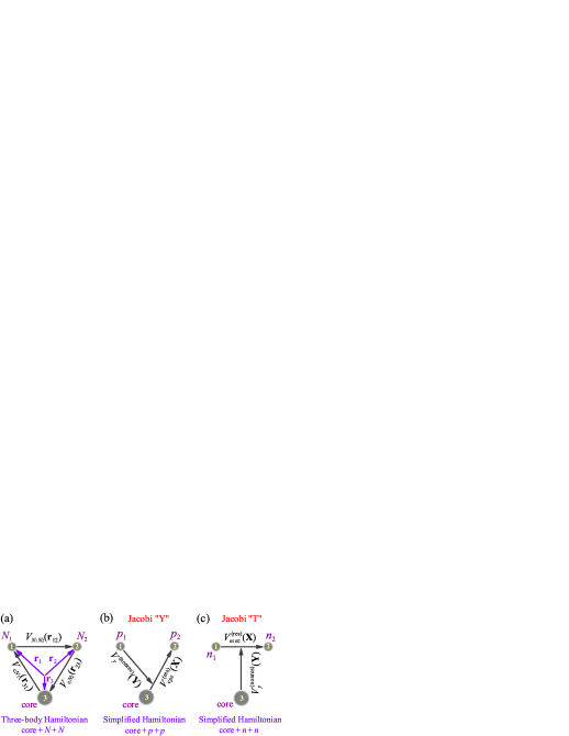
Fig. 1: Coordinate systems and potential sets for “hyperspherical harmonics” HH and “simplified Hamiltonian” SH approaches to ANC3. (a) The complete 3-body Hamiltonian is applied both to core+$p$+$p$ and core+$n$+$n$ systems. (b) For core+$p$+$p$ system the dynamical domination of lowest resonance in the core-$p$ subsystem motivates the use of simplified Hamiltonian in the “Y” Jacobi system. (c) For core+$n$+$n$ system the dynamical domination of the $n$-$n$ final state interaction motivates the use of simplified Hamiltonian in the “T” Jacobi system.

The continuum three-body problem is solved using the same Eq. (3) set but for continuum WF $\chi_{JK_{f}\gamma_{f},K_{f}^{\prime}\gamma_{f}^{\prime}}(\varkappa\rho)$ (square matrix of solutions) diagonalizing S-matrix. Hypermomentum $\varkappa$ is defined as $\varkappa=\sqrt{2ME_{T}}$. In the no-Coulomb case the WF is constructed by diagonalizing the $3\rightarrow 3$ elastic scattering S-matrix on asymptotics

$$\chi_{JK\gamma,K^{\prime}\gamma^{\prime}}(\varkappa\rho)=\exp(i\delta_{K\gamma,K^{\prime}\gamma^{\prime}})\sin(\varkappa\rho-(K+2)\pi/2$$

$$+\delta_{K\gamma,K^{\prime}\gamma^{\prime}})\,,\qquad S_{K\gamma,K^{\prime}\gamma^{\prime}}=\exp(2i\delta_{K\gamma,K^{\prime}\gamma^{\prime}})\,,$$

in analogy with the two-body case. This WF contains plane three-body wave and outgoing waves. The formulation of the boundary conditions becomes problematic in the Coulomb case and methods with only outgoing waves (including the SH model introduced later in Section 3) is a preferable choice. The details of the method and its applications are well explained in the literature [20, 21, 12, 22, 23, 19] and we will not dwell on that too much.

The form of hyperspherical equations (3) immediately provides the vision for the low-energy behavior of observables in E1 continuum since the only $K=1$ component with the lowest centrifugal barrier is important in the $E_{T}\rightarrow 0$ limit.

The E1 transitions between three-body cluster core+$N$+$N$ states are induced by the following operator

$$\mathcal{O}_{\text{E1},m}=e\,\sum\nolimits_{i=1,3}Z_{i}\,r_{i}\,Y_{1m}(\hat{r}_{i})=\sqrt{3/(4\pi)}\,D_{m}\,,$$

where $\mathbf{D}=\textstyle\sum_{i=1,3}eZ_{i}\mathbf{r}_{i}$ is the dipole operator, and

$$\mathcal{O}_{\text{E1},m}=Z_{\text{eff}}\,\rho\,\cos(\theta_{\rho})\,Y_{1m}(\hat{y})\,,$$ (4)

$$Z_{\text{eff}}^{2}=\left\{\begin{array}[]{l}Z^{2}_{3}\\ (Z_{3}-A_{3})^{2}\end{array}\right\}\frac{e^{2}\,(A_{1}+A_{2})}{A_{3}(A_{1}+A_{2}+A_{3})}\,.$$ (7)

The upper value in curly braces is for core+$n$+$n$ and the lower one is for core+$p$+$p$ three-body systems, taking into account the c.m. relation $\mathbf{r}_{1}+\mathbf{r}_{2}=-A_{3}\mathbf{r}_{3}$ for the three-body system.

For historical reasons the astrophysical E1 nonresonant radiative capture rate is expressed via the SF of the reciprocal E1 dissociation, see Eq. (49). The E1 dissociation SF in the HH approach is

$$\frac{dB_{E1}}{dE_{T}}=\sum\nolimits_{J_{f}}G_{fi}\,\sqrt{\frac{M}{2E_{T}}}\sum\nolimits_{K_{f}\gamma_{f}}|M_{J_{f}K_{f}\gamma_{f}}|^{2}\,.$$ (8)

where $J_{i}$ is total spin of bound state, $J_{f}$ is total spin of continuum state, $G_{fi}=(2J_{f}+1)/(2J_{i}+1)$ is a statistical factor, and the E1 matrix element is

$$M_{J_{f}K_{f}\gamma_{f}}=Z_{\text{eff}}\,{\sum\nolimits_{K_{f}^{\prime}\gamma_{f}^{\prime}}}{\sum\nolimits_{K_{i}\gamma_{i}}}M_{\text{a}}M_{\text{hh}}\int d\rho\,\sqrt{2/\pi}$$

$$\times\,\chi_{J_{f}K_{f}\gamma_{f},K_{f}^{\prime}\gamma_{f}^{\prime}}(\varkappa\rho)\,\rho\,\chi_{J_{i}K_{i}\gamma_{i}}(\rho)\,,$$

$$M_{\text{a}}=\left\langle J_{f}\gamma_{f}^{\prime}\left\|Y_{1}(\hat{y})\right\|J_{i}\gamma_{i}\right\rangle\,,\quad M_{\text{hh}}=\left\langle K_{f}^{\prime}\gamma_{f}^{\prime}\left|\cos(\theta_{\rho})\right|K_{i}\gamma_{i}\right\rangle\,.$$

For example, the reduced angular momentum matrix element $M_{\text{a}}=1/\sqrt{4\pi}$ for $J_{i}=0\rightarrow J_{f}=1$ transition and the hyperangular matrix element $M_{\text{hh}}=1/\sqrt{2}$ for $K_{i}=0\rightarrow K_{f}=1$ transition.

2.1 No Coulomb case in HH approach

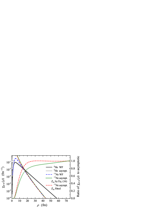
Fig. 2: Left axis: ground state WF components with $K=0$ for ⁶He (solid curve) and ¹⁷Ne (dashed curve), matched to asymptotic Bessel (thick gray curves) and Whittaker (short dashed and dotted curves) functions. For ⁶He ANC3 value is $\mathcal{C}_{3}=0.3$ $\text{fm}^{-1/2}$. For ¹⁷Ne ANC3 values are $\mathcal{C}_{3}=13400$ $\text{fm}^{-1/2}$ with $Z_{\text{hh}}=27.5$ [see Eq. (23)] and $\mathcal{C}_{3}=5958$ $\text{fm}^{-1/2}$ with fitted $Z_{\text{hh}}=26.14$. The lines on the right axis show the ratio of ¹⁷Ne WF to Whittaker functions with mentioned $Z_{\text{hh}}$ and $\mathcal{C}_{3}$.

For the three-body plane-wave case the solution matrix is diagonal and expressed in terms of cylindrical Bessel functions

$$\chi_{J_{f}K_{f}\gamma_{f},K_{f}^{\prime}\gamma_{f}^{\prime}}(\varkappa\rho)=\sqrt{\frac{2}{\pi}}\,\delta_{K_{f},K_{f}^{\prime}}\,\delta_{\gamma_{f},\gamma_{f}^{\prime}}\,\sqrt{\frac{\pi\varkappa\rho}{2}}\,J_{K_{f}+2}(\varkappa\rho)\,,$$

with asymptotics for small $\varkappa\rho$

$$\sqrt{\varkappa\rho}\,J_{K_{f}+2}(\varkappa\rho)\sim(\varkappa\rho)^{K_{f}+5/2}/[(K_{f}+2)!\,2^{K_{f}+2}]\,.$$ (9)

This expression can be used to separate the leading term of the low-energy dependence of the matrix element, labeled for simplicity only by the values of $K$ for the initial and final states

$$M_{K_{f}K_{i}}(E_{T}) = \sqrt{2/\pi}\,\varkappa^{K_{f}+5/2}Z_{\text{eff}}M_{\text{a}}M_{\text{hh}}I_{K_{f}K_{i}}(E_{T})\,,$$ (10)

$$I_{K_{f}K_{i}}(E_{T}) = \frac{1}{\varkappa^{K_{f}+2}}\int d\rho\,\rho^{3/2}\,J_{K_{f}+2}(\varkappa\rho)\,\chi_{J_{i}K_{i}\gamma_{i}}(\rho)\,.\qquad$$ (11)

where the overlap integral $I_{K_{f}K_{i}}$ tends to a constant at $E_{T}\rightarrow 0$ and weakly depends on energy in the range of interest.

Let us consider only the transition from the lowest bound state component $K_{i}=0$ to the lowest E1 continuum component with $K_{f}=1$:

$$\frac{dB_{E1}}{dE_{T}}=\frac{1}{\pi}\,G_{fi}\,Z^{2}_{\text{eff}}M^{2}_{\text{a}}M^{2}_{\text{hh}}\,(2M)^{4}\,E_{T}^{3}\,I^{2}_{10}(E_{T})\,.$$ (12)

Now we replace the bound state WF $\chi$ in Eq. (11) by its long-range asymptotics expressed in terms of the three-body ANC value $\mathcal{C}_{3}$ and cylindrical Bessel functions $K$

$$\chi_{K=0}(\rho)\rightarrow\mathcal{C}_{3}\,\sqrt{2\kappa\rho/\pi}\,K_{2}(\kappa\rho)\,,$$ (13)

where the g.s. hypermoment $\kappa=\sqrt{2ME_{\text{b}}}$ is defined via the binding energy $E_{\text{b}}$. This approximation is valid in a broad range of $\rho$ values, see Fig. 2. The ⁶He WF is taken from [19, 15]. The overlap integral now has simple analytical form

$$I_{10}(E_{T})=4\,\mathcal{C}_{3}\,/[(2ME_{\text{b}})^{11/4}(1+E_{T}/E_{\text{b}})^{2}]\,.$$ (14)

It can be found that the ANC3 approximation of the overlap value (14) deviates within very reasonable $\sim 7\%$ limits from the directly calculated by Eq. (11) in a broad energy range ($E_{T}\lesssim 1$ MeV).

2.2 Discussion of ⁶He case

The E1 SF and the astrophysical capture rate for the $\alpha$+$n$+$n\,\rightarrow\,^{6}$He+$\gamma$ was recently studied in Refs. [15, 19]. It can be found that Eq. (12) is not sufficient in this case for two reasons:

(i) In the $p$-shell ⁶He nucleus not only the $K_{i}=0\rightarrow K_{f}=1$ transition is important, but also $K_{i}=2\rightarrow K_{f}=1$. The asymptotics of the $K_{i}=2$ WF component falls off much faster than that of the component $K_{i}=0$. However, the weight of the $K_{i}=2$ WF component corresponding to $[p^{2}]$ configuration is much larger ($\sim 80\%$), than the weight of the $K_{i}=0$ WF component ($\sim 5\%$), due to Pauli-suppressed $[s^{2}]$ configuration. So, finally their contributions to the low-energy ME are comparable.

(ii) It was shown in [15, 19] that the low-energy part of the E1 SF is highly sensitive to the final state $n$-$n$ interaction (an increase in SF when the $n$-$n$ interaction is taken into account is a factor of 8). The paper [15] is devoted to the study of this effect in the dynamic dineutron model. We do not currently see a method to consider this effect analytically.

Applicability of the approximation (12) to the other cases of $2n$ capture should be considered separately.

2.3 Coulomb case in HH approach

Let us consider the transition to the single $K_{f}=1$ continuum final state. The low-energy behavior of continuum single channel WF in the Coulomb case is provided by the regular at the origin Coulomb WF

$$\chi_{K_{f}}(\varkappa\rho)\rightarrow\sqrt{2/\pi}\,F_{K_{f}+3/2}(\eta_{\text{hh}},\varkappa\rho)\,.$$ (15)

The suitable asymptotics of the Coulomb WFs are

$$F_{l}(\eta,kr) = \frac{(2l+1)!C_{l}(\eta)}{(2\eta)^{l+1}}\sqrt{2\beta r}\,I_{2l+1}(2\sqrt{2\beta r})\,,$$ (16)

$$G_{l}(\eta,kr) = \frac{2(2\eta)^{l}}{(2l+1)!C_{l}(\eta)}\sqrt{2\beta r}\,K_{2l+1}(2\sqrt{2\beta r})\,,$$ (17)

$$C_{l}(\eta) = 2^{l}\exp[-\pi\eta/2]\,\left|\Gamma[l+i\eta+1]\right|/\Gamma[2(l+1)]\,,\qquad$$ (18)

$$C^{\prime}_{l}(\eta) = \frac{\sqrt{\pi}(2\eta)^{l+1/2}}{(2l+1)!}\,\exp[-\pi\eta]\,,\qquad\beta=\eta k\,,$$ (19)

$$D_{l}(\eta,k) = \frac{(2l+1)!C^{\prime}_{l}(\eta)}{(2\eta)^{l+1}}\sqrt{2\beta}=\sqrt{\pi k}\,\exp[-\pi\eta]\,,\qquad$$ (20)

where $I$ and $K$ are modified Bessel functions. Approximation (19) for the Coulomb coefficient (18) works for $\eta\gg l$.

In the ANC3 approximation the g.s. WF $\chi$ can be replaced by its long-range asymptotics

$$\chi_{K_{i}}(\rho)\rightarrow\mathcal{C}_{3}\,W_{-\eta_{\text{gs}},K_{i}+2}(2\kappa\rho)\,.$$ (21)

This asymptotics is valid when all three particles are well separated. We will find out later that at least the core-$p$ distances, which contribute E1 SF, are simultaneously large, see Fig. 5 (b). The Sommerfeld parameters $\eta$ for continuum and bound states are

$$\eta_{\text{hh}}=\beta_{\text{hh}}/\varkappa\,,\quad\beta_{\text{hh}}=Z_{\text{hh}}e^{2}M\,,\quad\eta_{\text{gs}}=Z_{\text{hh}}\,e^{2}M/\kappa\,.$$ (22)

The effective charges of isolated hyperspherical channels can be defined as

$$Z_{\text{hh}}^{(Kl_{x}l_{y})}=\rho\left\langle Kl_{x}l_{y}\left|\frac{Z_{1}Z_{2}}{r_{12}}+\frac{Z_{2}Z_{3}}{r_{23}}+\frac{Z_{3}Z_{1}}{r_{31}}\right|Kl_{x}l_{y}\right\rangle.$$ (23)

For the ¹⁷Ne case the $K=0$ and $K=1$ effective charges are

$$Z_{\text{hh}}^{(000)}=27.50\,,\quad Z_{\text{hh}}^{(101)}=27.41\,.$$ (24)

Fig. 2 shows that the substitution Eq. (21) works well in a very broad range of radii (the ¹⁷Ne g.s. WF is from Ref. [24]). The effective charge in Eq. (24) obtained for $K_{i}=0$ is very reasonable. However, slightly different effective charge value $Z_{\text{hh}}^{(000)}=26.14$ is required for an almost perfect match to the asymptotics. This is a clear indication of coupled-channel dynamics in this case. It is actually a nontrivial fact that all the complexity of this dynamics reduces to a simple renormalization of effective charges.

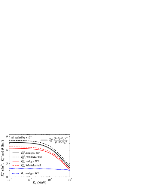
Fig. 3: Overlap integrals for HH $I^{(c)}_{10}(E_{T})$ [Eq. (25)], SH $I^{(cc)}_{10}(\varepsilon_{0},E_{T})$ [Eq. (33)], and $B(\varepsilon_{0},E_{T})$ [Eq. (46)]. The solid gray curve shows analytical approximation Eq. (40) for $I^{(cc)}_{10}$.

Using Eqs. (16) and (20) we can factorize the $E1$ matrix element as:

$$M_{K_{f}K_{i}}=\sqrt{2/\pi}\,D_{K_{f}+3/2}(\eta_{\text{hh}},\varkappa)\,M_{\text{a}}M_{\text{hh}}Z_{\text{eff}}\,I^{(c)}_{K_{f}K_{i}}(E_{T})\,,$$

$$I^{(c)}_{K_{f}K_{i}}(E_{T})=\int d\rho\,\frac{F_{K_{f}+3/2}(\eta_{\text{hh}},\varkappa\rho)}{D_{K_{f}+3/2}(\eta_{\text{hh}},\varkappa)}\,\rho^{3/2}\,\chi_{J_{i}K_{i}\gamma_{i}}(\rho)\,,\qquad$$ (25)

where the overlap integral $I^{(c)}_{K_{f}K_{i}}$ weakly depends on the energy and in the limit $E_{T}\rightarrow 0$ has a rather simple form

$$\tilde{I}^{(c)}_{K_{f}K_{i}}=\int d\rho\,I_{2l+1}(2\sqrt{2\beta_{\text{hh}}\rho})\,\rho^{3/2}\,\chi_{J_{i}K_{i}\gamma_{i}}(\rho)\,.$$ (26)

The overlaps (25) for $K_{i}=0\rightarrow K_{f}=1$ transition are shown in Fig. 3. It can be found that in the ANC3 approximation the Eq. (21) is quite accurate: in this case the overlap increases just less than $6\%$ compared the calculation with the real g.s. WF. It is also seen that the use of simple energy-independent overlap Eq. (26) instead of (25) gives almost perfect result below 10 keV and is reasonable below 100 keV. For the $E1$ SF we get:

$$\frac{dB_{E1}}{dE_{T}}=G_{fi}\,Z^{2}_{\text{eff}}M^{2}_{\text{a}}M^{2}_{\text{hh}}2MI^{(c)2}_{10}(E_{T})\exp[-2\pi\eta_{\text{hh}}]\,.$$ (27)

The energy dependence of the derived expression at $E_{T}\rightarrow 0$ is pure Coulomb exponent $\exp[-2\pi\eta_{\text{hh}}]$. The SF calculation results are shown in Fig. 4. They strongly disagree with calculation results from Refs. [13] and [14]. The modification of the “effective continuum charge” $Z_{\text{hh}}^{(101)}$ from Eq. (24) does not save the situation since the energy dependence of the SF in Eq. (27) and that of the SF in [13, 14] are too different. We demonstrate in the next section that the Eq. (27) is actually incorrect. However, the derivations of this section are still important for our further discussion.

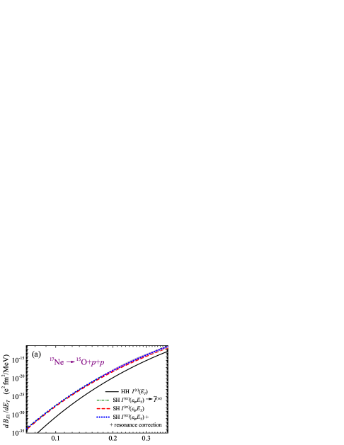
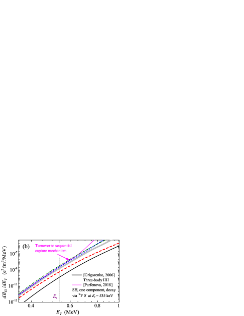
Fig. 4: The E1 strength functions for ¹⁷Ne $\rightarrow^{15}$O+$p$+$p$ transition. Solid black curve corresponds to E1 SF obtained with ANC3 HH method of Eq. (27). Green dash-dotted curve corresponds to simple energy-independent approximation Eq. (45) $I^{(cc)}(\varepsilon,E_{T})\rightarrow\tilde{I}^{(cc)}$. Red dashed and blue dotted curves corresponds to ANC3 SH method of Eq. (35) without and with the resonance correction Eq. (45), respectively. Thick gray curve and thin magenta solid curves correspond to SFs from Refs. [13] and [14], respectively.

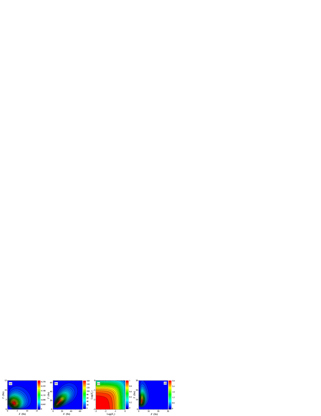
Fig. 5: (a) The WF $\psi_{\text{gs}}$ component with $K=0$, normalized to unity. (b) Integrand of Eq. (34). (c) $I^{(cc)}_{l_{x}l_{y}}(\varepsilon_{0},E_{T})/\tilde{I}^{(cc)}_{l_{x}l_{y}}$ on logarithmic axes. (d) Integrand of Eq. (46).

3 ANC3 in the simplified Hamiltonian (SH) approximation

The approximation is based on the usage of a simplified three-body Hamiltonian for the E1 continuum instead of the real one

$$\hat{H}_{3}\rightarrow\hat{H}^{\prime}_{3}=\hat{T}_{3}+V_{cN_{2}}(\mathbf{X})+V_{y}(\mathbf{Y})\,,$$ (28)

where $\mathbf{X}\equiv\mathbf{r}_{32}$ is the Jacobi vector in the “Y” Jacobi system, while $\mathbf{Y}$ corresponds to the second Jacobi vector, see Fig. 1. Such a Hamiltonian is quite reliable since the nuclear interaction with a proton in a non-natural parity state is weak. The model was used for nonresonant astrophysical rate calculations in ¹⁷Ne in Ref. [13] and in ⁶He in Ref. [15]. A thorough check of the model is given in Ref. [16], and the detailed description of the formalism for complicated angular momentum couplings in Ref. [14].

To obtain the E1 dissociation strength function in this approximation we solve the inhomogeneous Schrödinger equation

$$(\hat{H}^{\prime}_{3}-E_{T})\Psi_{M_{i}m}^{J_{f}M_{f}(+)}=\mathcal{O}_{\text{E1},m}\Psi^{J_{i}M_{i}}_{\text{gs}}\,,$$

for WF $\Psi^{(+)}$ with pure outgoing wave boundary conditions. The transition operator Eq. (4) dependent on $\mathbf{r}_{3}$ can be rewritten in $X$ and $Y$ coordinates using relation:

$$\mathbf{r}_{3}=\mathbf{X}\,A_{2}/(A_{2}+A_{3})-\mathbf{Y}\,A_{1}/(A_{1}+A_{2}+A_{3})\,.$$ (29)

Since the factorized form of the Hamiltonian Eq. (28) allows a semi-analytical expression for the three-body Green’s function, a rather simple expression for the SF can be obtained

$$\frac{dB_{E1}}{dE_{T}}=G_{fi}\,\frac{4}{\pi^{2}}\,E_{T}\int_{0}^{1}d\varepsilon\,\frac{M_{x}M_{y}}{k_{x}k_{y}}\,|A(E_{x},E_{y})|^{2}\,,\qquad$$ (30)

$$E_{x}=\varepsilon E_{T}\,,\quad E_{y}=(1-\varepsilon)E_{T}\,,\quad k_{x,y}=\sqrt{2M_{x,y}E_{x,y}}\,,$$

where $\varepsilon$ is the energy distribution parameter. The amplitude $A$ is defined as

$$A(E_{x},E_{y})=\int dXdY\,f_{l_{x}}(k_{x}X)\,f_{l_{y}}(k_{y}Y)\,\Phi(X,Y)\,.$$ (31)

where the “source function” $\Phi$ is defined by the E1 operator acting on $\Psi_{\text{gs}}$. The WFs $f_{l_{x}}$ and $f_{l_{y}}$ are eigenfunctions of sub-Hamiltonians depending on $X$ and $Y$ Jacobi coordinates in S-matrix representation with asymptotics

$$f_{l}(kr)=e^{i\delta_{l}}[F_{l}(\eta,kr)\cos(\delta_{l})+G_{l}(\eta,kr)\sin(\delta_{l})]\,.$$ (32)

Eq. (31) is given in a simplified form, neglecting angular momentum couplings, more details can be found in [14]. We skip this part of the formalism in this work. The calculations of the E1 strength function in the SH approximation without final state interactions in $X$ and $Y$ channels for the $2n$ capture are equivalent to calculations in the HH approximation. So, we skip no-Coulomb case and proceed to the $2p$ capture.

3.1 Coulomb case in SH approach

With good accuracy, one can calculate the amplitude only for the $Y$ coordinate and then double the result. This is not difficult to prove, but tedious, so we do not provide a proof here. The amplitude $A$ for the $Y$ coordinate [see Eq. (29)] from the transition operator Eq. (4) with extracted by Eqs. (16) and (20) low-energy dependence is written in terms of the overlap integral $I^{(cc)}$ as

$$A(E_{x},E_{y})=M_{\text{a}}D_{l_{x}}(\eta_{x},k_{x})\,D_{l_{y}}(\eta_{y},k_{y})\,I^{(cc)}_{l_{x}l_{y}}(\varepsilon,E_{T})\,,$$

$$I^{(cc)}_{l_{x}l_{y}}(\varepsilon,E_{T})=\int dXdY\frac{F_{l_{x}}(k_{x}X)}{D_{l_{x}}(\eta_{x},k_{x})}\frac{F_{l_{y}}(k_{y}Y)}{D_{l_{y}}(\eta_{y},k_{y})}Y\psi_{\text{gs}}(X,Y),\,$$ (33)

$$\eta_{x}=Z_{2}Z_{3}e^{2}M_{x}/k_{x}\,,\quad\eta_{y}=(Z_{2}+Z_{3})Z_{1}e^{2}M_{y}/k_{y}\,.$$

The asymptotic form of this overlap, independent of energy, is

$$\tilde{I}^{(cc)}_{l_{x}l_{y}} = \int dXdYI_{2l_{x}+1}(2\sqrt{2\beta_{x}X})I_{2l_{y}+1}(2\sqrt{2\beta_{y}Y})$$ (34)

$$\times \sqrt{XY^{3}}\,\psi_{\text{gs}}(X,Y)\,.$$

The WF $\psi_{\text{gs}}$ and the integrand of Eq. (33) on the $\{X,Y\}$ plane are shown in Figs. 5 (a) and (b). Their comparison illustrates the extreme peripheral character of the low-energy E1 transition: the WF maximum is at a distance of $\sim 3$ fm, while sizable contributions to the transition ME can be found up to $\sim 60$ fm.

The E1 SF with antisymmetry between nucleons taken into account is

$$\frac{dB_{E1}}{dE_{T}}=G_{fi}\,M^{2}_{\text{a}}\,4M_{x}M_{y}\frac{4(Z_{3}-A_{3})^{2}e^{2}(A_{2}+A_{3})^{2}}{(A_{1}+A_{2}+A_{3})^{2}A^{2}_{3}}\,I_{\varepsilon}(E_{T})\,,$$ (35)

$$I_{\varepsilon}(E_{T})=E_{T}\int_{0}^{1}d\varepsilon I^{(cc)2}_{10}(\varepsilon,E_{T})\exp[-2\pi(\eta_{x}+\eta_{y})]\,.\quad$$ (36)

The Coulomb exponent in $I_{\varepsilon}$ has a very sharp energy dependence, see Fig. 6. The energy dependence of $I^{(cc)}$ is shown in Fig. 5 (c): it is quite flat for $\varepsilon\approx\varepsilon_{0}$. Thus, $I^{(cc)}$ can be evaluated at the peak $\varepsilon=\varepsilon_{0}$ and the $\varepsilon$ integration can be performed by the saddle point method:

$$I_{\varepsilon}(E_{T})=I^{(cc)2}_{10}(\varepsilon_{0},E_{T})\,E_{T}\,\frac{\exp(-2\pi\eta_{\text{sh}})}{\sqrt{3R_{\varepsilon}\eta_{\text{sh}}}}\,,$$ (37)

$$\eta_{\text{sh}} = Z_{\text{sh}}e^{2}M/\varkappa\,,\quad Z_{\text{sh}}=(b_{x}+b_{y})^{3/2}\,,$$ (38)

$$\varepsilon_{0} = b_{x}/(b_{x}+b_{y})\,,\quad R_{\varepsilon}=(b_{x}+b_{y})^{2}/(4b_{x}b_{y})\,,$$

$$b_{x} = [Z_{3}^{2}Z_{2}^{2}M_{x}/M]^{1/3}\,,\quad b_{y}=[(Z_{3}+Z_{2})^{2}Z_{1}^{2}M_{y}/M]^{1/3}\,.$$

For the ¹⁷Ne $\rightarrow^{15}$O+$p$+$p$ transition

$$\varepsilon_{0}=0.48\,,\quad Z_{\text{sh}}=23.282\,,$$ (39)

The accuracy of the saddle point integration is $\sim 2\%$ and $\sim 6\%$ at 0.1 and 1 MeV, respectively.

It can be found in Fig. 3 that the analytical energy dependence of Eq. (14) obtained for the system without Coulomb interaction is still a good approximation in the considered Coulomb case,

$$I^{(cc)}_{10}(\varepsilon_{0},E_{T})=\tilde{I}^{(cc)}_{10}\frac{\sqrt{1+E_{T}/E_{\text{cy}}}}{(1+E_{T}/E_{\text{b}})^{2}}\,,\qquad E_{\text{cy}}=\frac{2M_{y}\beta_{y}}{1-\varepsilon_{0}}\,,\;$$ (40)

Eq. (40) contains additional Coulomb correction for $l_{y}=1$ motion in $Y$ coordinate (with $E_{\text{cy}}=3.67$ MeV) and we use it later for astrophysical rate derivation.

The results of the SF calculation in the SH approximation are shown in Fig. 4 by the red dashed curve. Now there is no significant disagreement for $E_{T}\rightarrow 0$ of the SH model results with calculation results from Refs. [13] and [14]. In the next Sections 3.2 and 3.3 we answer the following questions: (i) what is the reason for the difference between HH and SH ANC3 methods and (ii) can we get a better “fit” of the complicated three-body results in the SH approximation?

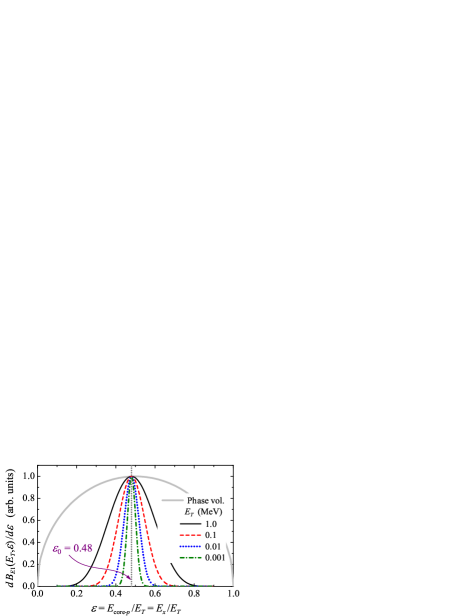
Fig. 6: Energy distribution between core and one of the protons for different decay energies $E_{T}$, governed by the $\exp[-2\pi(\eta_{x}+\eta_{y})]$ term in Eq. (36). All distributions are normalized to unity value at peak.

3.2 Correlated $2p$ emission/capture

In the HH Eq. (27) and SH Eq. (35) approximations we get SF expressions with the low-energy asymptotics

$$\frac{dB_{E1}}{dE_{T}}\propto\exp(-2\pi\eta_{\text{hh}})\,,\quad\frac{dB_{E1}}{dE_{T}}\propto E_{T}^{5/4}\exp(-2\pi\eta_{\text{sh}})\,,$$ (41)

which are qualitatively different. There are two main points. (i) Effective charge, entering the Coulomb exponent is significantly lower in SH case, see Eq. (39) compared to Eq. (24): 27.41 vs. 23.282. (ii) There is an additional power dependence on energy $E^{5/4}_{T}$ which, evidently, cannot be compensated, for example, by some modification of the effective charge. What is the source of qualitative difference between Eqs. (27) and (35)?

The answer is actually provided in Fig. 6: in the SH approach the emission of two protons is highly correlated process, which produces the narrow bell-shaped $\varepsilon$ distributions. In the approximation $K_{f}=1$ used in Eq. (27) the momentum distribution is described by the phase space (thick gray curve in Fig. 6). In the correlated calculation Eq. (35) this distribution is drastically modified by the three-body Coulombic effect. The momentum distribution which “shrinks” to the proximity of the $\varepsilon_{0}$ value allows an easier penetration, which is reflected also in the smaller effective charge (39) in the Coulomb exponent in Eq. (41).

So, what is wrong with Eq. (27)? Formally the transition by the dipole operator from $K_{i}=0$ g.s. occurs only to $K_{f}=1$ continuum, as we assumed. This means that the substitution of Eq. (15) is incorrect. This substitution is based on the assumption that for $E_{T}\rightarrow 0$ only the component with minimal possible $K_{f}=1$ and, hence, the smallest centrifugal barrier, contributes to the penetrability. Now it is clear that for the three-body continuum Coulomb problem this “evident” argument is incorrect. Within the complete HH couple-channel problem the $K_{f}=1$ channel should be affected by an infinite sum of the other channels in such a way that their cumulative effect does not vanish even in the limit $E_{T}\rightarrow 0$.

Analogous energy correlation effect is well known for the $2p$ radioactivity process. It was predicted by Goldansky in his pioneering work on $2p$ radioactivity [25]: in the Coulomb-correlated emission of two protons the energies of the protons tend to be equal in the limit of infinitely strong Coulomb interaction in the core+$p$ channel. This effect for two-proton radioactivity and resonant “true” two-proton emission is now well studied experimentally and understood in details in theoretical calculations [23, 26]. It is proved that the approximations like Eq. (35) represent well the underlying physics of the phenomenon.

3.3 Effect of a resonant state in a two-body subsystem

It was shown in calculations of [13, 14] (see Figs. 3 and 4-5 in these works) that the resonant state in the core-$p$ subsystem with “natural parity” quantum numbers significantly affects both the profile of the E1 strength function in a wide range of energies and the asymptotic behavior at low $E_{T}$ values. To evaluate the influence of resonance on the asymptotics analytically, let us consider the two-body resonant scattering WF in the quasistationary approximation:

$$f_{l}(kr)=e^{i\delta_{l}}F_{l}(kr)\cos(\delta_{l})+\frac{\sqrt{v\,\Gamma(E)}/2}{E_{r}-E-i\Gamma(E)/2}\tilde{\psi}_{l}(r)\,.\;$$ (42)

This expression can be easily connected with the asymptotics Eq. (32) by using the resonant R-matrix formulas:

$$\tan(\delta_{l})=\frac{\Gamma(E)}{E_{r}-E}\;\rightarrow\;e^{i\delta_{l}}\sin(\delta_{l})=\frac{\Gamma(E)/2}{E_{r}-E+i\Gamma(E)/2}\,.$$ (43)

The $\tilde{\psi}_{l}(r)$ is so-called quasistationary WF, defined at resonant energy $E_{r}$ by the irregular Coulomb WF boundary condition and normalized to unity in the “internal region” $r<r_{c}$:

$$\tilde{\psi}_{l}(r_{c})\stackrel{{\scriptstyle E=E_{r}}}{{\propto}}G_{l}(k_{r}r_{c})\,,\quad\int_{0}^{r_{c}}dr|\tilde{\psi}_{l}(r)|^{2}=1\,.$$ (44)

The low-energy behavior of the overlap integrals Eq. (33) with the resonant continuum WF (42) in $X$ coordinate is then

$$I^{(cc)\prime}_{l_{x}l_{y}}(\varepsilon_{0},E_{T})=I^{(cc)}_{l_{x}l_{y}}(\varepsilon_{0},E_{T})+\frac{B(\varepsilon_{0},E_{T})}{1-\varepsilon_{0}E_{T}/E_{r}}\,,\quad$$ (45)

$$B(\varepsilon_{0},E_{T})=B_{c}\int dXdY\tilde{\psi}_{l_{x}}(X)\frac{F_{l_{y}}(\eta_{y},k_{y}Y)}{D_{l_{y}}(\eta_{y},k_{y})}Y\psi_{\text{gs}}(X,Y)\,,$$ (46)

$$B_{c}=\theta_{x}\,[4M_{x}r_{c}K_{2l_{x}+1}(2\sqrt{2\beta_{x}r_{c}})E_{r}]^{-1}\,.\quad$$

Here we use the R-matrix width definition

$$\Gamma(E)=\frac{\theta^{2}}{Mr^{2}_{c}}\,P_{l}(E,r_{c})\,,\;P_{l}(E,r_{c})=\frac{kr_{c}}{F^{2}_{l}(kr_{c})+G^{2}_{l}(kr_{c})}\,,$$ (47)

which is simplified in the low-energy region using Eq.  (17).

The integrand of Eq. (46) is shown in Fig. 5 (d) and it has quite peripheral character compared to the g.s. WF Fig. 5 (a). The “resonance correction function” $B$ is shown in Fig. 3 demonstrating very weak dependence on energy. It is evaluated with function $\tilde{\psi}_{l_{x}}(X)$ approximated by Hulten Ansatz with rms $X$ value 3.5 fm. Parameters $\theta_{x}=1$ and $r_{c}=3.7$ fm allows to reproduce correctly the experimental width $\Gamma=25(5)$ keV of the ¹⁶F $0^{-}$ ground state at $E_{r}=535$ keV. So, in the whole energy range of interest we can approximate $B$ as

$$\tilde{B}=B(\varepsilon_{0},E_{T}\rightarrow 0)\,.$$ (48)

The blue dotted curve in Fig. 4 shows nice agreement of the “resonance corrected” E1 SF with complete three-body calculations up to $\sim 600$ keV. At this energy the two-body resonance well enters the “energy window” for three-body capture $E_{r}<E_{T}$ and turnover to sequential capture mechanism is taking place.

3.4 Astrophysical rate calculations

The nonresonant radiative capture rate is expressed via the SF of E1 dissociation Eq. (8) as

$$\left\langle\sigma_{2p,\gamma}v\right\rangle = \left(\frac{\textstyle\sum_{n}A_{n}}{A_{1}A_{2}A_{3}}\right)^{3/2}\left(\frac{2\pi}{mkT}\right)^{3}\,\frac{2J_{f}+1}{2(2J_{i}+1)}\,I_{E}(T)\,,\;$$

$$I_{E}(T) = \int dE\,\frac{16\pi}{9}\,E_{\gamma}^{3}\;\frac{dB_{E1}(E)}{dE}\exp\left[-\frac{E}{kT}\right]\,,$$ (49)

where $J_{i}$ and $J_{f}$ are spins of the ¹⁵O and ¹⁷Ne g.s., respectively [14].

The energy dependence of Eq. (35) is too complex to allow a direct analytical calculation of the astrophysical capture rate. However, using Eqs. (37), (40), and (48), the main analytical terms can be obtained by the saddle point calculation near the Gamow peak energy $E_{G}$:

$$I_{E}(T)\propto\int dE_{T}(E_{\text{b}}+E_{T})^{3}I_{\varepsilon}(E_{T})\exp\left[-\frac{E_{T}}{kT}\right]=\frac{2\pi E_{\text{b}}^{3}E_{\text{G}}^{5/2}}{3\gamma\sqrt{R_{\varepsilon}}}$$

$$\times\frac{1+E_{\text{G}}/E_{\text{cy}}}{1+E_{\text{G}}/E_{\text{b}}}\left(\tilde{I}^{(cc)}_{10}+\frac{(1+E_{\text{G}}/E_{\text{b}})^{2}}{1-\varepsilon_{0}E_{\text{G}}/E_{r}}\tilde{B}\right)^{2}\exp\left[-\frac{3\gamma^{2/3}}{(kT)^{1/3}}\right],\,$$

$$E_{\text{G}}=(\gamma kT)^{2/3}\,,\quad\gamma=\pi Z_{\text{sh}}e^{2}\sqrt{M/2}\,,\quad\pi\eta_{\text{sh}}=\gamma/\sqrt{E_{T}}\,.\quad$$ (50)

The Gamow peak energy can be found as $\{0.05,0.21,1\}$ MeV at $\{0.01,0.1,1\}$ GK. Comparison of the rates calculated in a model of the paper Ref. [14] and in this work is given in Fig. 7. It can be seen that even the very crude energy-independent approximation Eq. (34) $I^{(cc)}(\varepsilon,E_{T})\rightarrow\tilde{I}^{(cc)}$ for $T<0.5$ GK works well within a factor of 2. The energy-dependent calculations Eq. (45) are nearly perfect for $T<0.2$ GK and the analytical expression Eq. (50) for the rate is a very good approximation to numerically computed rate for $T<0.4$ GK.

The low-temperature dependence of the nonresonant $2p$ capture rate is

$$\langle\sigma_{2p,\gamma}\,v\rangle\propto\mathcal{C}^{2}_{3}\,T^{5/3}\,\exp[-(T_{\text{eff}}/T)^{1/3}]\,,\quad kT_{\text{eff}}\approx 193\;\text{MeV}\,.$$

Analogous dependence for the resonant rate is (e.g. Ref. [12])

$$\langle\sigma_{2p,\gamma}\,v\rangle\propto\Gamma_{2p}\,T^{-3}\,\exp[-(E_{3r}/kT)]\,,\quad E_{3r}=0.355\;\text{MeV}\,,$$

where $E_{3r}$ is the lowest state decaying via $2p$ emission with $\Gamma_{2p}$ (for ¹⁷Ne this is the first excited $3/2^{-}$ state). Here it can be found that nonresonant capture dominates in the low-temperature limit, see also discussion in Ref. [13].

So, we have obtained a compact analytical expression for the $2p$ capture rate, which depends only on the global parameters of the system under consideration ($\mathcal{C}_{3}$, $E_{\text{b}}$, $E_{r}$, $Z_{\text{sh}}$) and two universal overlaps ($\tilde{I}^{(cc)}$ and $\tilde{B}$) calculated at $E_{T}\rightarrow 0$.

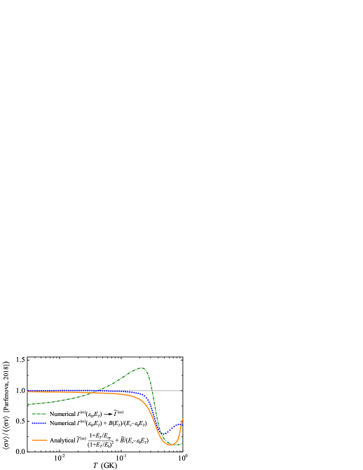
Fig. 7: Ratio of the rates for astrophysical nonresonant three-body capture reaction ¹⁵O+$p$+$p\rightarrow^{17}$Ne+$\gamma$ obtained in this work and in the paper [14] (see the thin magenta solid line SF in Fig. 4). Blue dotted and solid orange curve show the results of numerical rate calculation by Eq. (49) and analytical result by Eq. (50) for the resonance-corrected $I^{(cc)\prime}(\varepsilon,E_{T})$ from Eq. (45). Green dash-dotted curve shows the rate for simple energy-independent SF $I^{(cc)}(\varepsilon,E_{T})\rightarrow\tilde{I}^{(cc)}$ from Eq. (34).

4 General note on three-body Coulomb continuum problem

The three-body Coulomb continuum problem is a famous long-term conundrum of theoretical and mathematical physics. Complexity of this problem is defined by the possible presence of the Coulomb correlations, bound and resonant states in the two-body subsystems. As a result, no compact analytical form of the asymptotics is known for the three-body Coulomb continuum problem. There is known approximate asymptotic solution of this problem (so-called “Redmond-Merkuriev” asymptotics) [27, 28], which is valid in four regions: in one region all three particles are far from each other $r_{12}\sim r_{23}\sim r_{31}$ and there are three regions where different pairs of three particles are close $r_{ij}\ll r_{jk}\sim r_{ki}$. There were fruitful applications of this asymptotics, e.g. to atomic problems [29, 30]. There is a wide range of works dedicated to improvement of this asymptotics [31, 32, 33, 34]. One of modern trends is not to struggle with analytical problems of this asymptotics, but to use powerful computing and propagate numerical solutions to distances where uncertainties of the asymptotics does not play a practical role. However, we do not think that this is a completely satisfactory approach, which should replace the analytical developments.

In this work we deal with a limited subset of the three-body Coulomb continuum problem: only repulsive Coulomb interactions and no bound states in the subsystems. Specific feature of our problem is that the three-body energies are extremely small and the solution residue in the kinematical region, where the contributions of two two-body Coulomb asymptotics (core-$p_{1}$ and core-$p_{2}$ channels) overlap, see Fig. 8 (a). This justifies amplitude factorization and consequent analytical calculations of Section 3.1. However, reliability of this approximation is based on the fact that $p$-$p$ Coulomb interaction is quite small compared to core-$p$ interaction. It can be found from Fig. 8 (b) that a minor part of the kinematical space is affected by the $p$-$p$ repulsion for energies $1<E_{T}<1000$ keV important for astrophysics. It should be understood, that, rigorously speaking, for some extreme $E_{T}\rightarrow 0$ the correlations induced by $p$-$p$ Coulomb interaction will become important in the whole kinematical plane $\{\varepsilon,\cos(\theta_{k})\}$ and the low-energy asymptotics, which we deduced in this work, will be broken.

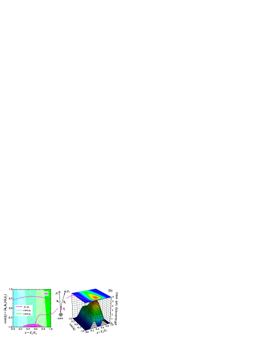
Fig. 8: (a) Regions in the kinematical plane $\{\varepsilon,\cos(\theta_{k})\}$ where effects of the two-body Coulomb repulsion are dominating. Different colors correspond to different pairs of particles, where $r_{ij}\ll r_{jk}\sim r_{ki}$. Solid color corresponds to $E_{T}\sim 1$ MeV [to be compared with panel (b)], hatched regions to $E_{T}\sim 1-100$ keV. The dotted magenta curve illustrates the region of $p$-$p$ repulsion dominance at some hypothetical extremely small energy $E_{T}\ll 1$ keV. (b) Illustration of the Coulomb repulsion dominance regions by example of theoretical momentum distribution for decay ¹⁶Ne(g.s.)$\rightarrow^{14}$O+$p$+$p$ with $E_{T}=1.466$ MeV, very well reproducing the data [26].

5 Conclusion

In this paper, we provide a formalism for a complete analytical description of low-energy three-body $2p$ nonresonant radiative capture processes. The developed approach is a generalization of the ANC method, which has proven itself well for two-body nonresonant radiative captures. The ordinary (two-body) ANC2 method demonstrates the sensitivity of the low-energy E1 strength function, important for astrophysics, to only two parameters: the binding energy $E_{\text{b}}$ and the ANC2 value $\mathcal{C}_{2}$. For the three-body ANC3 method one more parameter should be employed: the energy $E_{r}$ of the lowest to the threshold “natural parity” two-body resonance with appropriate quantum numbers.

An interesting formal result is related to the problem of the three-body Coulomb interaction in the continuum. We demonstrate that ANC3 method developed completely in three-body hyperspherical harmonics representation (named “HH approximation”) is not valid in the Coulomb case as it gives incorrect low-energy asymptotics of SF and hence incorrect low-temperature asymptotics of the astrophysical rate. The reason for this is the highly correlated nature of the $2p$ capture. The correct asymptotics can be obtained using the Coulomb-correlated SH approximation based on a simplified three-body Hamiltonian. The latter approximation also allows to determine the correction related to the low-lying two-body resonant state in the core-nucleon channel.

The two-dimensional overlap integrals involved in the ANC3 approximation in the correlated Coulomb case are rather complicated compared to those in the ANC2 case. However, their calculation is a task that is incomparably simpler than any complete three-body calculation. The whole formal framework is compact and elegant and requires only two overlap calculations: $\tilde{I}^{(cc)}$ and $\tilde{B}$. Thus, we find that ANC3 approximation in a three-body case is a valuable development providing robust tool for estimates of the three-body nonresonant capture rates in the low-temperature ($T\lesssim 0.3-1$ GK) domain.

Acknowledgments. — LVG, YLP, and NBS were supported in part by the Russian Science Foundation grant No. 17-12-01367.

References

- [1] H.M. Xu, C.A. Gagliardi, R.E. Tribble, A.M. Mukhamedzhanov, N.K. Timofeyuk, Phys. Rev. Lett. 73 (1994) 2027–2030.
- [2] N. K. Timofeyuk, R. C. Johnson, A. M. Mukhamedzhanov, Phys. Rev. Lett. 91 (2003) 232501.
- [3] D.Y. Pang, F.M. Nunes, A.M. Mukhamedzhanov, Phys. Rev. C 75 (2007) 024601.
- [4] J. Okołowicz, N. Michel, W. Nazarewicz, M. Płoszajczak, Phys. Rev. C 85 (2012) 064320.
- [5] A.M. Mukhamedzhanov, Phys. Rev. C 99 (2019) 024311.
- [6] L.D. Blokhintsev, I. Borbely, E.I. Dolinskii, Sov. J. Part. Nucl. 8 (1977) 485.
- [7] A.M. Mukhamedzhanov, L.D. Blokhintsev, B.A. Brown, V. Burjan, S. Cherubini, C.A. Gagliardi, B.F. Irgaziev, V. Kroha, F.M. Nunes, F. Pirlepesov, R.G. Pizzone, S. Romano, C. Spitaleri, X.D. Tang, L. Trache, R.E. Tribble, A. Tumino, Eur. Phys. J. A 27 (2006) 205–215.
- [8] A.M. Mukhamedzhanov, G.V. Rogachev, Phys. Rev. C 96 (2017) 045811.
- [9] A.M. Mukhamedzhanov, D.Y. Pang, A.S. Kadyrov, Phys. Rev. C 99 (2019) 064618.
- [10] W. Fowler, G. Caughlan, B. Zimmerman, Annual Review of Astronomy and Astrophysics 5 (1967) 525.
- [11] C. Angulo, M. Arnould, M. Rayet, P. Descouvemont, D. Baye, C. Leclercq-Willain, A. Coc, S. Barhoumi, P. Aguer, C. Rolfs, R. Kunz, J. Hammer, A. Mayer, T. Paradellis, S. Kossionides, C. Chronidou, K. Spyrou, S. del’Innocenti, G. Fiorentini, B. Ricci, S. Zavatarelli, C. Providencia, H. Wolters, J. Soares, C. Grama, J. Rahighi, A., Shotter, M. L. Rachti, Nucl. Phys. A 656 (1999) 3–183.
- [12] L. V. Grigorenko, M. V. Zhukov, Phys. Rev. C 72 (2005) 015803.
- [13] L. Grigorenko, K. Langanke, N. Shul’gina, M. Zhukov, Physics Letters B 641 (2006) 254–259.
- [14] Y.L. Parfenova, L.V. Grigorenko, I.A. Egorova, N.B. Shulgina, J.S. Vaagen, M.V. Zhukov, Phys. Rev. C 98 (2018) 034608.
- [15] L. Grigorenko, N. Shulgina, M. Zhukov, Physics Letters B 807 (2020) 135557.
- [16] L.V. Grigorenko, M.V. Zhukov, Phys. Rev. C 76 (2007) 014008.
- [17] L.V. Grigorenko, M.V. Zhukov, Phys. Rev. C 76 (2007) 014009.
- [18] L.V. Grigorenko, J.S. Vaagen, M.V. Zhukov, Phys. Rev. C 97 (2018) 034605.
- [19] L.V. Grigorenko, N.B. Shulgina, M.V. Zhukov, Phys. Rev. C 102 (2020) 014611.
- [20] M.V. Zhukov, B. Danilin, D. Fedorov, J. Bang, I. Thompson, J.S. Vaagen, Phys. Rep. 231 (1993) 151–199.
- [21] L.V. Grigorenko, R.C. Johnson, I.G. Mukha, I.J. Thompson, M.V. Zhukov, Phys. Rev. C 64 (2001) 054002.
- [22] L.V. Grigorenko, T.D. Wiser, K. Mercurio, R.J. Charity, R. Shane, L.G. Sobotka, J.M. Elson, A.H. Wuosmaa, A. Banu, M. McCleskey, L. Trache, R.E. Tribble, M.V. Zhukov, Phys. Rev. C 80 (2009) 034602.
- [23] M. Pfützner, M. Karny, L.V. Grigorenko, K. Riisager, Rev. Mod. Phys. 84 (2012) 567–619.
- [24] L. Grigorenko, I. Mukha, M. Zhukov, Nuclear Physics A 713 (2003) 372–389.
- [25] V.I. Goldansky, Nucl. Phys. 19 (1960) 482–495.
- [26] K.W. Brown, R.J. Charity, L.G. Sobotka, L.V. Grigorenko, T.A. Golubkova, S. Bedoor, W.W. Buhro, Z. Chajecki, J.M. Elson, W.G. Lynch, J. Manfredi, D.G. McNeel, W. Reviol, R. Shane, R.H. Showalter, M.B. Tsang, J.R. Winkelbauer, A.H. Wuosmaa, Phys. Rev. C 92 (2015) 034329.
- [27] L. Rosenberg, Phys. Rev. D 8 (1973) 1833–1843.
- [28] S.P. Merkuriev, Teor. Mat. Fiz. 32 (1977) 187; Theor. Math. Phys. 32 (1977) 680.
- [29] R.K. Peterkop and L.L. Rabik, Teor. Mat. Fiz. 31 (1977) 502.
- [30] M. Brauner, J.S. Briggs, H.J. Klar, J. Phys. B 22 (1989) 2265.
- [31] E.O. Alt and A.M. Mukhamedzhanov, Phys. Rev. 47 (1993) 2004.
- [32] A.M. Mukhamedzhanov, A.S. Kadyrov, F. Pirlepesov, Phys. Rev. A 73 (2006)012713.
- [33] A.S. Kadyrov, I. Bray, A.M. Mukhamedzhanov, A.T. Stelbovics, Annals of Physics 324 (2009) 1516.
- [34] S.L. Yakovlev, Theor. Math. Phys., 203 (2020) 664–672.