A parallel-in-time algorithm for high-order BDF methods for diffusion and subdiffusion equations

Abstract

In this paper, we propose a parallel-in-time algorithm for approximately solving parabolic equations. In particular, we apply the $k$-step backward differentiation formula, and then develop an iterative solver by using the waveform relaxation technique. Each resulting iteration represents a periodic-like system, which could be further solved in parallel by using the diagonalization technique. The convergence of the waveform relaxation iteration is theoretically examined by using the generating function method. The approach we established in this paper extends the existing argument of single-step methods in Gander and Wu [Numer. Math., 143 (2019), pp. 489–527] to general BDF methods up to order six. The argument could be further applied to the time-fractional subdiffusion equation, whose discretization shares common properties of the standard BDF methods, because of the nonlocality of the fractional differential operator. Illustrative numerical results are presented to complement the theoretical analysis.

1 Introduction

The aim of this paper is to develop a parallel-in-time (PinT) solver for high-order time stepping schemes of diffusion models. We begin with the normal diffusion, which is described by parabolic equations.

Let $V\subset H=H^{\prime}\subset V^{\prime}$ be a Gelfand triple of complex Hilbert spaces. Namely, the embedding $V\hookrightarrow H$ is continuous and dense, and

$$\langle u,v\rangle=(u,v),\quad\forall\,u\in H\hookrightarrow V^{\prime},\,\,\forall\,v\in V\hookrightarrow H,$$

where $\langle\cdot,\cdot\rangle$ is the duality pairing between $V^{\prime}$ and $V$, and $(\cdot,\cdot)$ is the inner product on $H$. Throughout, we let $\|\cdot\|$ and $\|\cdot\|_{V}$ denote the norms of the space $H$ and $V$, respectively.

Let $T>0$, $v\in H$, $f\in L^{2}(0,T;V^{\prime})$, and consider the initial value problem of seeking $u\in L^{2}(0,T;V)\cap H^{1}(0,T;V^{\prime})\hookrightarrow C([0,T];H)$ such that

$$\left\{\begin{aligned} \partial_{t}u(t)+Au(t)&=f(t),\quad\text{for all}~{}~{}t\in(0,T],\\ u(0)&=v,\end{aligned}\right.$$ (1)

where $A:V\to V^{\prime}$ is a self-adjoint bounded linear operator with the following elliptic property:

$$\beta_{0}\|u\|_{V}^{2}\leq\langle Au,u\rangle\leq\beta_{1}\|u\|_{V}^{2},\forall\,u\in V,$$ (2)

with constants $\beta_{1}>\beta_{0}>0$. For example, if we consider a heat equation on a bounded Lipschitz domain $\Omega\subset\mathbb{R}^{d}$ and $A$ denotes negative Laplacian $-\Delta$ with homogeneous Dirichlet boundary conditions, then $H=L^{2}(\Omega)$ and $V=H_{0}^{1}(\Omega)$.

In recent years, the development and analysis of parallel algorithms for solving evolution problems have attracted a lot of attention. The first group of parallel schemes is based on the inverse Laplace transform, which represents the solution as a contour integral in the complex plane and a carefully designed quadrature rule [34, 46, 53, 58]. Such a method is directly parallelizable and accurate even for a nonsmooth problem data. However, this strategy is not directly applicable for the nonlinear problem or anomalous diffusion problems with time-dependent diffusion coefficients. To the second group belongs the widely used parareal algorithm [4, 13, 15, 43, 60], which could be derived as a multigrid-in-time method or a multiple shooting method in the time direction. See also the space-time multigrid method [22, 24, 40, 59, 56]. We refer the interested reader to survey papers [11, 51] and references therein.

Very recently, in [16], Gander and Wu developed a novel PinT algorithm, by applying the waveform relaxation [47, 49] and a diagonalization technique [42, 14, 18]. In particular, they proposed a simple iteration: for given $u_{m-1}(T)\in H$, look for $u_{m}$ such that

$$\left\{\begin{aligned} \partial_{t}u_{m}(t)+Au_{m}(t)&=f(t),\quad\text{for all}~{}~{}t\in(0,T];\\ u_{m}(0)&=v+\kappa(u_{m}-u_{m-1})(T).\end{aligned}\right.$$ (3)

Here $\kappa$ denotes a relaxation parameter. Note that the exact solution $u$ is a fixed point of the iteration (3). It was proved in [16, Theorem 3.1] that, by selecting a proper $\kappa\in(0,1)$, the iteration (3) converges with the convergence factor ${\kappa e^{-cT}}/{(1-\kappa e^{-cT})}$, where $c$ is the smallest eigenvalue of $A$ and $c\geq\beta_{0}$.

Then, a direct discretization of (3) by the backward Euler method immediately results in a periodic-like discrete system, and therefore the diagonalization technique is applicable here to carry out a direct parallel computation. The diagonalization technique was firstly proposed by Maday and Rønquist for solving evolution models [42]. The basic idea is to reformulate the time-stepping system into a space-time all-at-once system, then diagonalize the time stepping matrix and solve all time steps in parallel. The computational cost of each iteration is proved to be $O([MN\log(N)+\widetilde{M}_{f}N]/p)$ for each processor, where $M,N$ are numbers of degree of freedoms in space and time respectively, $\widetilde{M}_{f}$ is the computational cost for solving a Poisson-like problem obtained by diagonalization, and $p$ is the number of used processors. In particular, Gander and Wu considered single-step $\theta$-methods for solving (3) with uniform step size [16, Section 3.2]. The convergence analysis of the discrete system was also established, where the proof is similar to the argument for the continuous problem.

With $\varepsilon$ being the desired error tolerance, a $k$-th order time stepping scheme requires $N=O(\varepsilon^{-1/k})$ time steps. Therefore, the computational complexity for each processor turns out to be $O([(\widetilde{M}_{f}+M|\log(\varepsilon)|/k)\varepsilon^{-1/k}]/p)$. Besides, the roundoff error of the algorithm is proved to be $O(\epsilon\kappa^{-2}N^{2})=O(\epsilon\kappa^{-2}\varepsilon^{-2/k})$, where $\epsilon$ is the machine precision; see more details in Section 3.2. Those facts motivate us to develop and analyze PinT schemes for (1), by using some high-order time stepping schemes, such as the $k$-step backward differentiation formula (BDF$k$) with $k=2,3,\ldots,6$, and the aforementioned waveform relaxation technique. This is beyond the scope of all existing references [12, 16] which only focus on $\theta$-methods, and represents the main theoretical achievements of the work.

Instead of directly discretizing (3), we start with the time stepping schemes of (1) using BDF$k$ with uniform step size $\tau=T/N$. Then, by perturbing the discrete problem, we obtain a periodic-like system in each iteration, which can be parallelly solved by using $O([MN\log(N)+\widetilde{M}_{f}N]/p)$ operations (for each processor). We prove that the resulting iteration linearly converges to the exact solution (with a proper choice of the relaxation parameter $\kappa$), by using the generating function technique as well as the decay property of discrete solution operator. Specifically, let $U_{m}^{n}$ be the solution of the $m$-th iteration of the perturbed iterative system with the initial guess $U_{0}^{n}=v$ for all $0\leq n\leq N$, and $u$ be the exact solution to (1). Provided certain data regularity, we show the error estimate for all $1\leq n\leq N$ (Theorem 7):

$$\|U_{m}^{n}-u(t_{n})\| \leq c(\gamma(\kappa)^{m}+\tau^{k}t_{n}^{-k}),\quad\text{with}~{}~{}\kappa\in(0,1)~{}\text{independent of}~{}\tau,$$

where the positive constant $c$ and the convergence factor (23)

$$\gamma(\kappa)=\frac{c\kappa e^{-c_{1}T}}{1-c\kappa e^{-c_{1}T}}\in(0,1)$$

might depend on $k$, $\kappa$, $\beta_{0}$, $T$, $v$ and $f$, but it is independent of $\tau$, $n$, $m$ and $u$. Therefore, to attain the discretization error $O(\tau^{k})$ or $O(N^{-k})$, the computational complexity for each processor is $O(\log(N)[MN\log(N)+\widetilde{M}_{f}N]/p)$.

The above argument could be extended to the subdiffusion model, that involves a time-fractional derivative of order $\alpha\in(0,1)$. Let $T>0$, $v\in H$, $f\in L^{p}(0,T;V^{\prime})$ with $p\in(2/\alpha,\infty)$, and consider the initial value problem of seeking $u\in L^{p}(0,T;V)\cap H^{\alpha}(0,T;V^{\prime})$ such that

$$\left\{\begin{aligned} \partial_{t}^{\alpha}u(t)+Au(t)&=f(t),\quad\text{for all}~{}~{}t\in(0,T],\\ u(0)&=v.\end{aligned}\right.$$ (4)

Here $\partial_{t}^{\alpha}u$ denotes the left-sided Caputo fractional derivative of order $\alpha$, defined by

$$\partial_{t}^{\alpha}u(t):=\frac{1}{\Gamma(1-\alpha)}\int_{0}^{t}(t-s)^{-\alpha}u^{\prime}(s)\,ds,$$ (5)

The interest in (4) is motivated by its excellent capability of modeling anomalously slow diffusion, such as protein diffusion within cells [19], thermal diffusion in media with fractal geometry [50], and contaminant transport in groundwater [32], to name but a few. The literature on the numerical approximation for the subdiffusion equation (4) is vast. The most popular methods include convolution quadrature [8, 29, 5, 10], collocation method [65, 54, 36, 33], discontinuous Galerkin method [44, 48, 45], and spectral method [7, 25, 64]. See also [3, 27, 37, 17, 61] for some fast algorithms.

Our argument for linear multistep schemes could be easily applied to many popular time stepping schemes for the subdiffusion problem (4). As an example, we consider the convolution quadrature generated by BDF$k$ method, which was established by Lubich’s series of work [38, 39]. Note that the fractional derivative is nonlocal-in-time, and hence its discretization inherits the nonlocality and behaves like a multistep discretization with an infinitely-wide stencil. By perturbing the time stepping scheme, we develop an iterative algorithm that requires a periodic-like system to be solved in each iteration, which could be parallelly solved by a diagonalization technique with $O([MN\log(N)+\widetilde{M}_{f}N]/p)$ operations for each processor. Moreover, error estimates of the resulting numerical schemes are established by using the decay property of the (discrete) solution operator. We prove the following error estimate (Theorem 14):

$$\|U_{m}^{N}-u(t_{N})\| \leq c(\gamma(\kappa)^{m}+\tau^{k}t_{n}^{-k}),\qquad\text{with}\quad\kappa=O(1/\log(N)),$$

where $U_{m}^{n}$ is the solution to the iterative algorithm (33) with the initial guess $U_{0}^{n}=v$ for all $0\leq n\leq N$, and $u$ is the exact solution to the subdiffusion problem (4). In the estimate, the positive constant $c$ and the convergence factor

$$\gamma(\kappa)=\frac{c\kappa\log(N)}{1-c\kappa\log(N)}\in(0,1)$$

might depend on $\alpha$, $k$, $\kappa$, $\beta_{0}$, $T$, $v$ and $f$, but they are always independent of $\tau$, $n$, $m$ and $u$. The analysis is promising for some nonlinear evolution equations as well as (sub-)diffusion problems involving time-dependent diffusion coefficients. See a very recent work of Gu and Wu [21] for a parallel algorithm by using the diagonalization technique, where the analysis only works for BDF$2$ with $\alpha<5/8$.

The rest of the paper is organized as follows. In Section 2, we develop a high-order time parallel schemes for solving the parabolic problem and analyze its convergence by generating function technique. In Section 3, we extend our discussion to the nonlocal-in-time subdiffusion problem. Finally, in Section 4, we present some numerical results to illustrate and complement the theoretical analysis.

2 Parallel algorithms for normal diffusion equations

The aim of this section is to propose high-order multistep PinT schemes, with rigorous convergence analysis, for approximately solving the parabolic equation (1).

2.1 BDF$k$ scheme for normal diffusion equations

We consider the BDF$k$ scheme, $k=1,2,\ldots,6$, with uniform step size. Let $\{t_{n}=\tau n\}$ be a uniform partition of the interval $[0,T]$, with a time step size $\tau=T/N$. For $n\geq 1$, the $k$-step BDF scheme seeks $U^{n}\in V$ such that [35]

$$\bar{\partial}_{\tau}U^{n}+AU^{n} =f(t_{n})+a_{n}^{(k)}(f(0)-Av)+\sum_{\ell=1}^{k-2}b_{\ell,n}^{(k)}\tau^{\ell}\partial_{t}^{\ell}f(0)=:\bar{f}_{n},$$ (6)

$$U^{-(k-1)} =\cdots=U^{-1}=U^{0}=v.$$

In (6) we use the BDF$k$ to approximate the first-order derivative by

$$\bar{\partial}_{t}U^{n}:=\frac{1}{\tau}\sum_{j=0}^{k}\omega_{j}U^{n-j},$$

where constants $\{\omega_{j}\}$ are coefficients of the polynomials

$$\delta_{k}(\zeta):=\sum_{\ell=1}^{k}\frac{1}{\ell}(1-\zeta)^{\ell}=\sum\limits^{k}_{j=0}\omega_{j}\zeta^{j}.$$ (7)

For $\alpha=1$, the BDF$k$ scheme is known to be $A(\vartheta_{k})$-stable with angle $\vartheta_{k}=90^{\circ}$, $90^{\circ}$, $86.03^{\circ}$, $73.35^{\circ}$, $51.84^{\circ}$, $17.84^{\circ}$ for $k=1,2,3,4,5,6$, respectively [23, pp. 251].

To apply the BDF$k$ for parabolic problem, it is well-known that one need starting data $U^{j}=u(t_{j})+O(\tau^{k})$ for $0\leq j\leq k-1$. Then the error bound of the time stepping scheme is $O(\tau^{k})$. However, for nonlocal-in-time subdiffusion models (which will be discussed in section 3), the knowledge of $U^{j}$ for $0\leq j\leq k-1$ does not guarantee an error bound $O(\tau^{k})$. It is due to the lack of compatibility of problem data. Fortunately, in the preceding work of the second author and his colleagues, it was proved that one can recover the optimal error bound $O(\tau^{k})$ by modifying the starting $k-1$ steps [29]. The strategy also works for the BDF$k$ for classical parabolic equations [35]. In order to keep consistency with numerical schemes for subdiffusion models, we decide to apply the modified formulation (6) of the BDF$k$.

Table 1: The coefficients $a_{n}^{(k)}$ and $b_{\ell,n}^{(k)}$.

$k$	$a_{1}^{(k)}$	$a_{2}^{(k)}$	$a_{3}^{(k)}$	$a_{4}^{(k)}$	$a_{5}^{(k)}$	$\ell$	$b_{\ell,1}^{(k)}$	$b_{\ell,2}^{(k)}$	$b_{\ell,3}^{(k)}$	$b_{\ell,4}^{(k)}$	$b_{\ell,5}^{(k)}$
$k=2$	$\frac{1}{2}$
$k=3$	$\frac{11}{12}$	$-\frac{5}{12}$				$\ell=1$	$\frac{1}{12}$	0
$k=4$	$\frac{31}{24}$	$-\frac{7}{6}$	$\frac{3}{8}$			$\ell=1$	$\frac{1}{6}$	$-\frac{1}{12}$	$0$
						$\ell=2$	$0$	$0$	$0$
$k=5$	$\frac{1181}{720}$	$-\frac{177}{80}$	$\frac{341}{240}$	$-\frac{251}{720}$		$\ell=1$	$\frac{59}{240}$	$-\frac{29}{120}$	$\frac{19}{240}$	$0$
						$\ell=2$	$\frac{1}{240}$	$-\frac{1}{240}$	$0$	$0$
						$\ell=3$	$\frac{1}{720}$	$0$	$0$	$0$
$k=6$	$\frac{2837}{1440}$	$-\frac{2543}{720}$	$\frac{17}{5}$	$-\frac{1201}{720}$	$\frac{95}{288}$	$\ell=1$	$\frac{77}{240}$	$-\frac{7}{15}$	$\frac{73}{240}$	$-\frac{3}{40}$	0
						$\ell=2$	$\frac{1}{96}$	$-\frac{1}{60}$	$\frac{1}{160}$	$0$	0
						$\ell=3$	$-\frac{1}{360}$	$\frac{1}{720}$	$0$	$0$	0
						$\ell=4$	$0$	$0$	$0$	$0$	0

The next lemma provides some properties of the generating function. The proof has been provided in [29, Theorem A.1], and hence omitted here.

Lemma 1.

For any $\varepsilon$, there exists $\theta_{\varepsilon}\in(\pi/2,\pi)$ such that for any $\theta\in(\pi/2,\theta_{\varepsilon})$, there holds $\delta_{k}(e^{-z})\in\Sigma_{\pi-\vartheta_{k}+\varepsilon}$ for any $z\in\Gamma_{\theta}^{\pi/\sin{\theta}}=\{z=re^{\pm i\theta},~{}0\leq r\leq\pi/\sin\theta\}$, where $\Sigma_{\psi}:=\{z\in\mathbb{C}:~{}|\arg(z)|\leq\psi\}$. Meanwhile, there exist positive constants $c_{0}$ and $c_{0}^{\prime}$ such that

$$c_{0}|z|\leq|\delta_{k}(e^{-z})|\leq c_{0}^{\prime}|z|\qquad\forall~{}z\in\Gamma_{\theta}^{\pi/\sin{\theta}}.$$

For $n\geq k$, we choose $a_{n}^{(k)}$ and $b_{\ell,n}^{(k)}$ to be zero. Then $\bar{\partial}_{\tau}u(t_{n})$ is the standard approximation of $\partial_{t}u(t_{n})$ by BDF$k$. For $1\leq n\leq k-1$, these constants have been determined in [29, 35], cf. Table 1. In particular, if

$$v\in H\quad\text{and}\quad f\in W^{k,1}(0,T;H)\cap C^{k-1}([0,T];H),$$ (8)

the numerical solution to (6) satisfies the following error estimate. We omit the proof here and refer interested readers to [35, Theorem 1.1] and [29, Theorem 2.1] for error analysis of (non-selfadjoint) parabolic systems and fractional subdiffusion equations, respectively.

Lemma 2.

Assume that the problem data $v$ and $f$ satisfy (8), then

$$\|U^{n}-u(t_{n})\|\leq c\,\tau^{k}\bigg{(}t_{n}^{-k}\|v\|+\sum_{\ell=0}^{k-1}t_{n}^{\ell-k+1}\|\partial_{t}^{\ell}f(0)\|+\int_{0}^{t_{n}}\|\partial_{s}^{k}f(s)\|ds\bigg{)},$$ (9)

where the constant $c$ is independent of $\tau$ and $n$.

2.2 Development of parallel-in-time algorithm

Next, we develop a PinT algorithm for (6): for given $U_{m-1}^{n}$, $N-k+1\leq n\leq N$, we compute $U_{m}^{n}$ by

$$\bar{\partial}_{\tau}U_{m}^{n}+AU_{m}^{n} =\bar{f}_{n},~{}\quad\qquad\qquad\qquad\qquad n=1,2,\cdots,N,$$ (10)

$$U_{m}^{-j} =v+\kappa(U_{m}^{N-j}-U_{m-1}^{N-j}),\quad j=0,1,\ldots,k-1,$$

where the revised source term $\bar{f}_{n}$ is given in (6). Note that the exact time stepping solution $\{U^{n}\}_{n=1}^{N}$ is a fixed point of this iteration. In Section 2.4, we provide a systematic framework to study the iterative algorithm (10), which also works for the time-fractional subdiffusion problem discussed later.

We may rewrite the BDF$k$ scheme (10) in the following matrix form:

$$\frac{1}{\tau}(B_{k}(\kappa)\otimes I_{x}){\bf U}_{m}+(I_{t}\otimes A){\bf U}_{m}={\bf F}_{m-1},$$ (11)

where ${\bf U}_{m}=(U_{m}^{1},U_{m}^{2},\cdots,U_{m}^{N})^{T}$, ${\bf F}_{m-1}=(F_{1},F_{2},\cdots,F_{N})^{T}$ with

$$F_{n}:=\bar{f}_{n}+\frac{\kappa}{\tau}\sum_{j=1}^{n}\omega_{j}U_{m-1}^{N-j+1}+\frac{1}{\tau}\sum_{j=0}^{n-1}\omega_{j}v,$$ (12)

and

$$B_{k}(\kappa)=\begin{bmatrix}\omega_{0}&\cdots&0&\kappa\omega_{k}&\cdots&\kappa\omega_{2}&\kappa\omega_{1}\\ \omega_{1}&\omega_{0}&&0&\kappa\omega_{k}&\cdots&\kappa\omega_{2}\\ \vdots&\vdots&&&&\ddots&\vdots\\ \vdots&\vdots&&\ddots&&0&\kappa\omega_{k}\\ \omega_{k}&\omega_{k-1}&\cdots&&&&0\\ 0&\omega_{k}&\omega_{k-1}&\cdots&&&\vdots\\ &&&\ddots&\ddots&&\vdots\\ &&0&\omega_{k}&\cdots&\omega_{1}&\omega_{0}\end{bmatrix}.$$

Here, we recall that $\omega_{j}=0$ if $j>k$ and $\sum_{j=0}^{k}\omega_{j}=0$ for the normal diffusion equations. The following lemma is crucial for the design of PinT algorithm.

Lemma 3 (Diagonalization).

Let $\Lambda(\kappa)=\mathrm{diag}(1,\kappa^{-\frac{1}{N}},\cdots,\kappa^{-\frac{N-1}{N}})$, then

$$B_{k}(\kappa)=\Lambda(\kappa)\tilde{B}_{k}(\kappa)\Lambda(\kappa)^{-1},$$

where the circular matrix $\tilde{B}_{k}(\kappa)$ has the form

$$\tilde{B}_{k}(\kappa)=\begin{bmatrix}\omega_{0}&0&\kappa^{\frac{k}{N}}\omega_{k}&\cdots&\kappa^{\frac{2}{N}}\omega_{2}&\kappa^{\frac{1}{N}}\omega_{1}\\ \kappa^{\frac{1}{N}}\omega_{1}&\omega_{0}&0&\kappa^{\frac{k}{N}}\omega_{k}&\cdots&\kappa^{\frac{2}{N}}\omega_{2}\\ \vdots&\vdots&&&\ddots&\vdots\\ \vdots&\vdots&\ddots&&0&\kappa^{\frac{k}{N}}\omega_{k}\\ \kappa^{\frac{k}{N}}\omega_{k}&\kappa^{\frac{k-1}{N}}\omega_{k-1}&\cdots&&&0\\ 0&\kappa^{\frac{k}{N}}\omega_{k}&\kappa^{\frac{k-1}{N}}\omega_{k-1}&\cdots&\\ &&&\ddots&\ddots&\vdots\\ &0&\kappa^{\frac{k}{N}}\omega_{k}&\cdots&\kappa^{\frac{1}{N}}\omega_{1}&\omega_{0}\end{bmatrix}.$$

As a consequence, $B_{k}(\kappa)$ can be diagonalized by

$$B_{k}(\kappa)=S(\kappa)D_{k}(\kappa)S(\kappa)^{-1},\quad S(\kappa):=\Lambda(\kappa)V,$$

where the Fourier matrix

$$V=[v_{1},v_{2},\ldots,v_{N}],\quad\text{with}\quad v_{n}=\big{[}1,\mathrm{e}^{i\frac{2(n-1)\pi}{N}},\ldots,\mathrm{e}^{i\frac{2(n-1)(N-1)\pi}{N}}\big{]}^{T},$$ (13)

and $D_{k}(k)$ is a diagonal matrix.

Using the above lemma, we can solve the system (10) in a parallel-in-time manner.

Algorithm 1   PinT algorithm by diagonalization technique for diffusion equation.

1:  Solve $(S(\kappa)\otimes I_{x}){\bf H}={\bf F}_{m-1}$.

2:  Solve $({D}_{k}(\kappa)\otimes I_{x}+\tau I_{t}\otimes A){\bf Q}=\tau{\bf H}$.

3:  Solve $(S(\kappa)^{-1}\otimes I_{x}){\bf U}_{m}={\bf Q}$.

It is known that the circulant matrix can be diagonalized by FFT with $\mathcal{O}(N\log N)$ operations [20, Chapter 4.7.7]. Then in each iteration, it turns out to be $N$ independent Poisson-like equations, which can be efficiently solved by, for instance, the multigrid method.

Speedup analysis of Algorithm 1

Let $M_{f}$ be the total real floating point operations for solving the (elliptic) Poisson-like equations. Then the cost for the serial computation is $O(M_{f}N)$. It is known that with (optimal) multigrid method $M_{f}$ is proportional to $M$, the number of degrees of freedom in space.

Consider the parallelization of Algorithm 1 with $p$ processors. The Step 1 and Step 3 can be finished with the total computational cost $O([MN\log(N)]/p)$ by using the bulk synchronous parallel FFT algorithm [26], see also [16, Section 4.1] for the detailed analysis. We note here that the ${\bf F}$ in (12) needs to be updated via ${\bf U}_{m-1}$, whose computational cost is $O(M)$ since $\omega_{j}=0$ when $j>k$. The PinT algorithm of ${\bf F}$ will be more delicate for the time-fractional subdiffusion problem discussed later.

For the Step 2, the total computational cost is $O((\widetilde{M}_{f}N)/p)$, where $\widetilde{M}_{f}$ denotes total real floating point operations for solving the Poisson-like equations obtained by diagonalization, and hence the cost for the parallel computation is $O([MN\log(N)+\widetilde{M}_{f}N]/p)$. In case that $p=O(N)$, then the parallel computational cost reduces to $O(M\log(N)+\widetilde{M}_{f})$. In some cases, $\widetilde{M}_{f}$ could be (almost) linear to $M$ even in higher dimensions. For example, if we consider the heat equation with periodic boundary conditions, we can apply FFT to solve the Poinsson-like equations with computational complexity $\widetilde{M}_{f}=O(M\log M)$.

With $\varepsilon$ being the desired error tolerance, a $k$-th order time stepping scheme requires $N=O(\varepsilon^{-1/k})$ time steps. Then, in order to attain sufficient accuracy $O(\varepsilon)$, the number of iterations should be $O(\log N)$, because the convergence factor $\gamma(\kappa)\in(0,1)$ is independent of $N$ (cf. Theorem 2.7). Therefore, the total computational cost is $O([MN(\log N)^{2}+\widetilde{M}_{f}N\log N]/p)$.

Remark 2.1.

The proposed algorithm uses FFT to diagonalize over time. It transforms the parabolic PDE into a decoupled set of elliptic PDEs. Such a technique is quite common for solving time-periodic problems, but relatively new for solving initial value problems.

In this paper, we only discuss the parallelism in the time direction. Nevertheless, combining the proposed method with some parallel-in-space algorithms, one may obtain an algorithm with polylog parallel complexity if $O(MN)$ processors were available. For example, for parabolic equations with periodic boundary conditions, one may apply FFT to transform the parabolic PDE into a decoupled set of ODEs:

$$u_{j}^{\prime}(t)+\lambda_{j}u_{j}(t)=f_{j}(t),\quad\text{with}~{}~{}u_{j}(0)=v_{j},$$

where $1\leq j\leq M$ and $M$ denotes the number of degree of freedoms in space. Then, these decoupled ODEs could be efficiently solved by using the parallel-in-time algorithm proposed in this paper.

Roundoff error of Algorithm 1

Let ${\bf{U}}_{m}$ be the exact solution of (11), and ${\bf{\widehat{U}}}_{m}$ be the solution of Algorithm 1. We assume that the Step 2 of Algorithm 1 is solved in a direct manner (for example, the LU factorization). Then for simplicity, we consider an arbitrary eigenvalue of the matrix $A$ and analyze the relative roundoff error. To this end, we replace matrices $I_{x}$ and $A$ by scalars $1$ and $\mu$. Then the system (11) reduces to

$$B{{\bf{U}}_{m}}=F,\quad\text{with}\quad B=\frac{1}{\tau}B_{k}(\kappa)+\mu I_{t}.$$

Then by Lemma 3, we define

$$D=S(\kappa)^{-1}BS(\kappa),\quad\text{and hence}\quad D=\frac{1}{\tau}D_{k}(\kappa)+\mu I_{t}.$$

Note that to solve $B{{\bf{U}}_{m}}=F$ by diagonalization is equivalent to solving $(B+\delta B){{\bf{\widehat{U}}}_{m}}=F$ with some perturbation $\delta B$, which can be easily bounded by [16, p. 496]

$$\|\delta B\|_{2}\leq\epsilon(2N+1)\|S(\kappa)\|_{2}\|S(\kappa)^{-1}\|_{2}\|D\|_{2}+O(\epsilon^{2}),$$

where $\epsilon$ denotes the machine precision ($\epsilon=2.2204\times 10^{-16}$ for a 32-bit computer). Then the roundoff error satisfies

$$\begin{split}\frac{\|{{\bf{U}}_{m}}-{{\bf{\widehat{U}}}_{m}}\|_{2}}{\|{{\bf{U}}_{m}}\|_{2}}&\leq\text{cond}_{2}(B)\frac{\|\delta B\|_{2}}{\|B\|_{2}}\leq\epsilon(2N+1)\|S(\kappa)\|_{2}\|S(\kappa)^{-1}\|_{2}\|D\|_{2}\|B^{-1}\|_{2}\\ &\leq\epsilon(2N+1)\,\text{cond}_{2}(S(\kappa))^{2}\,\text{cond}_{2}(D).\end{split}$$

Here we note that for $\kappa\in(0,1]$

$$\begin{split}\|S(\kappa)\|_{2}\leq\|\Lambda(\kappa)\|_{2}\|V\|_{2}\leq\kappa^{-\frac{N-1}{N}}\sqrt{N},\end{split}$$

and

$$\begin{split}\|S(\kappa)^{-1}\|_{2}\leq\|\Lambda(\kappa)^{-1}\|_{2}\|V^{-1}\|_{2}\leq\frac{1}{\sqrt{N}}.\end{split}$$

Therefore, we arrive at

$$\begin{split}\text{cond}_{2}(S(\kappa))=\|S(\kappa)\|_{2}\|S(\kappa)^{-1}\|_{2}\leq\kappa^{-\frac{N-1}{N}}\leq\kappa^{-1}.\end{split}$$

For the diagonal matrix $D$

$$\begin{split}\|D^{-1}\|_{2}&=\max_{1\leq n\leq N}\Big{|}\frac{1}{\tau}\delta_{k}(\kappa^{\frac{1}{N}}e^{-\mathrm{i}\frac{2(n-1)\pi}{N}})+\mu\Big{|}^{-1}\leq(\sin\theta_{k}\mu)^{-1}.\end{split}$$

Here we apply $A(\theta_{k})$ stability of the BDF$k$ scheme with $\theta_{k}\in(0,\pi/2)$. Similarly, using the definition of generating function (7), we derive for any $\kappa\in(0,1)$ and $N>1$

$$\begin{split}\|D\|_{2}&=\max_{1\leq n\leq N}\Big{|}\frac{1}{\tau}\delta_{k}(\kappa^{\frac{1}{N}}e^{-\mathrm{i}\frac{2(n-1)\pi}{N}})+\mu\Big{|}\leq\frac{1}{\tau}\delta_{k}(-\kappa^{\frac{1}{N}})+\mu\leq\frac{1}{\tau}\delta_{k}(-\kappa^{\frac{1}{N}})+\mu.\end{split}$$ (14)

Hence, we obtain

$$\begin{split}\text{cond}_{2}(D)&\leq\Big{(}\frac{\delta_{k}(-1)}{\tau}+\mu\Big{)}(\mu\sin\theta_{k})^{-1}.\end{split}$$

As a result, we have for $\mu\in[\mu_{0},\infty)$ (where the positive number $\mu_{0}$ depends on $\beta_{0}$ in (2))

$$\frac{\|{{\bf{U}}_{m}}-{{\bf{\widehat{U}}}_{m}}\|_{2}}{\|{{\bf{U}}_{m}}\|_{2}}\leq\epsilon(2N+1)\kappa^{-2}\Big{(}\frac{\delta_{k}(-1)}{\tau}+\mu\Big{)}(\mu\sin\theta_{k})^{-1}\leq C_{k}\epsilon\kappa^{-2}N^{2},$$ (15)

where the constant $C_{k}$ can be written as

$$C_{k}=3\Big{(}1+\Big{[}\frac{\delta_{k}(-1)}{T}\Big{]}/\mu_{0}\Big{)}(\sin\theta_{k})^{-1}.$$

It only depends on the order of BDF method and $\beta_{0}$ in (2). Note that the bound of roundoff error is uniform for $\mu\rightarrow\infty$, therefore it holds for all self-adjoint operators $A$ satisfying (2).

Remark 2.2.

The above analysis shows a reasonable estimate that roundoff error is $O(\epsilon\kappa^{-2}N^{2})$. See a similar estimates for some A-stable single-step methods like backward Euler scheme or Crank–Nicolson scheme [16]. The difference is that the BDF$k$ scheme (with $k>2$) is no longer A-stable. In our numerical experiments, we indeed observe that the roundoff error increases as $N\rightarrow\infty$.

2.3 Representation of numerical solution

The aim of this section is to develop the representation of the numerical solution of the $k$-step BDF schemes through a contour integral in complex domain, and to establish decaying properties of the solution operators.

By letting $W^{n}=U^{n}-v$, we can reformulate the time stepping scheme (6) as

$$\bar{\partial}_{\tau}W^{n}+AW^{n} =-Av+\bar{f}_{n},\quad n=1,2,\cdots,N,$$ (16)

$$W^{-(k-1)} =\cdots=W^{-1}=W^{0}=0.$$

By multiplying $\xi^{n}$ on (16) and taking summation over $n$ ( we extend $n$ in (16) to infinity in sense that $\bar{f}_{n}=0$ with $n\geq N$), we have

$$\sum_{n=1}^{\infty}\xi^{n}\bar{\partial}_{t}W^{n}+\sum_{n=1}^{\infty}\xi^{n}AW^{n}=-\sum_{n=1}^{\infty}\xi^{n}Av+\bar{f}_{n}\xi^{n}.$$

For any given sequence $\{V^{n}\}_{n=0}^{\infty}$, let $\widetilde{V}(\xi):=\sum_{n=0}^{\infty}V^{n}\xi^{n}$ denote its generating function. Since $W^{-(k-1)}=\cdots=W^{-1}=W^{0}=0$, according to properties of discrete convolution, we have the identity

$$\sum_{n=1}^{\infty}\xi^{n}\bar{\partial}_{\tau}V_{n}=\frac{\delta_{k}(\xi)}{\tau}\widetilde{V}(\xi),$$

where $\delta_{k}(\xi)$ denotes the generating function of the $k$-step BDF method (7). Therefore we conclude that

$$\Big{(}\frac{\delta_{k}(\xi)}{\tau}+A\Big{)}\widetilde{W}(\xi)=-\Big{(}\frac{\xi}{1-\xi}\Big{)}Av+\widetilde{\bar{f}_{n}}(\xi),$$

which implies that

$$\widetilde{W}(\xi)=\Big{(}\frac{\delta_{k}(\xi)}{\tau}+A\Big{)}^{-1}\Big{[}-\Big{(}\frac{\xi}{1-\xi}\Big{)}Av+\widetilde{\bar{f}_{n}}(\xi)\Big{]}.$$

It is easy to see that $\widetilde{W}(\xi)$ is analytic with respect to $\xi$ in the circle $|\xi|=\rho$, for $\rho>0$ small, on the complex plane, then with Cauchy’s integral formula, we have the following expression

$$W^{n} =\frac{1}{2\pi\mathrm{i}}\int_{|\xi|=\rho}\xi^{-n-1}\widetilde{W}(\xi){\rm d}\xi$$

$$=\frac{\tau}{2\pi\mathrm{i}}\int_{|\xi|=\rho}\xi^{-n-1}\Big{(}\delta_{k}(\xi)+\tau A\Big{)}^{-1}\Big{[}-\Big{(}\frac{\xi}{1-\xi}\Big{)}Av+\widetilde{\bar{f}_{n}}(\xi)\Big{]}{\rm d}\xi.$$

Therefore we obtain the solution representation:

$$U^{n}=(I+F_{\tau}^{n})v+\tau\sum_{j=1}^{n}E_{\tau}^{n-j}\bar{f}_{j}.$$ (17)

where the discrete operators $F_{\tau}^{n}$ and $E_{\tau}^{n}$ are respectively defined by

$$F_{\tau}^{n} =-\frac{1}{2\pi\mathrm{i}}\int_{|\xi|=\rho}\frac{1}{\xi^{n}(1-\xi)}\Big{(}\delta_{k}(\xi)/\tau+A\Big{)}^{-1}A\,{\rm d}\xi,$$ (18)

$$E_{\tau}^{n} =\frac{1}{2\pi\tau\mathrm{i}}\int_{|\xi|=\rho}\xi^{-n-1}\Big{(}\delta_{k}(\xi)/\tau+A\Big{)}^{-1}\,{\rm d}\xi.$$

Now we recall a useful estimate (cf. [55, Lemma 10.3]). For $k=1,\cdots,6$, there are positive constants $c,C$ and $\lambda_{0}$ (only depends on the BDF$k$ method) such that

$$\Big{|}\frac{1}{2\pi\mathrm{i}}\int_{|\xi|=\rho}\xi^{-n-1}(\delta_{k}(\xi)+\lambda)^{-1}\,{\rm d}\xi\Big{|}\leq~{}\left\{\begin{aligned} &Ce^{-cn\lambda},\quad 0<\lambda\leq\lambda_{0},\\ &C\lambda^{-1}e^{-cn},\quad\lambda>\lambda_{0}.\end{aligned}\right.$$ (19)

This together with the coercivity property (2) immediately implies the following lemma.

Lemma 4.

Let $E_{\tau}^{n}$ be the discrete operator defined in (18). Then

$$\|E_{\tau}^{n}\|_{H\rightarrow H}\leq c_{2}e^{-c_{1}t_{n}}.$$

Here the generic positive constants $c_{1}$ and $c_{2}$ are independent of $n$ and $\tau$.

2.4 Convergence analysis

In this section, we analyze the convergence of the iterative scheme (10), or equivalently,

$$\bar{\partial}_{\tau}U_{m}^{n}+AU_{m}^{n} =\bar{f}_{n}-\frac{\kappa}{\tau}G^{n}_{m},\quad n=1,2,\ldots,N,$$ (20)

$$U_{m}^{-j} =v,\qquad\qquad\quad j=0,1,\ldots,k-1.$$

where the term $G^{n}_{m}$ is given by

$$G^{n}_{m}=\sum_{j=n}^{k}\omega_{j}\left(U_{m}^{N+n-j}-U_{m-1}^{N+n-j}\right).$$ (21)

Here, the summation is assumed to vanish if the lower bound is greater than the upper bound. We aim to show that $U_{m}^{N}$ converges to $U^{N}$, the solution of the time stepping scheme (6), as $m\rightarrow\infty$.

Lemma 5.

Let $U_{m}^{n}$ be the solution to the iterative scheme (10) with $v=0$ and $\bar{f}_{n}=0$ for all $n=1,2,\ldots.N$. Then we can choose a proper parameter $\kappa>0$ in (10), which is independent of step size $\tau$, such that the following estimate holds valid:

$$\sum_{j=0}^{k-1}\|U_{m}^{N-j}\|\leq\gamma(\kappa)\sum_{j=0}^{k-1}\|U_{m-1}^{N-j}\|.$$

Here $\gamma(\kappa)\in(0,1)$, is constant depending on $\kappa$, $\beta_{0}$ and $T$, but independent of $\tau$.

Proof.

Following the preceding argument in Section 2.3, $U_{m}^{n}$ could be represented by

$$U_{m}^{n} =-\kappa\sum_{i=1}^{n}E_{\tau}^{n-i}G_{m}^{i}$$ (22)

$$=-\kappa\sum_{i=1}^{\min\{k,n\}}E_{\tau}^{n-i}\sum_{j=i}^{k}\omega_{j}(U_{m}^{N+i-j}-U_{m-1}^{N+i-j}),\quad n=1,2,\ldots,N.$$

Now we take the $H$ norm in (22) and apply Lemma 4 to obtain

$$\sum_{j=0}^{k-1}\|U_{m}^{N-j}\| \leq c\kappa e^{-c_{1}T}\sum_{j=0}^{k-1}\|U_{m}^{N-j}-U_{m-1}^{N-j}\|.$$

where $c$ is a generic constant and $c_{1}$ is the constant in Lemma 4. Then we apply the triangle inequality, by choosing $\kappa$ small enough such that $c\kappa e^{-c_{1}T}<1$, and hence derive that

$$\sum_{j=0}^{k-1}\|U_{m}^{N-j}\| \leq\frac{c\kappa e^{-c_{1}T}}{1-c\kappa e^{-c_{1}T}}\sum_{j=0}^{k-1}\|U_{m-1}^{N-j}\|.$$

Finally, we define the convergence factor

$$\gamma(\kappa):=\frac{c\kappa e^{-c_{1}T}}{1-c\kappa e^{-c_{1}T}}.$$ (23)

Then by choose $\kappa$ sufficiently small such that $c\kappa e^{-c_{1}T}\in(0,1/2)$, we have $\gamma(\kappa)\in(0,1)$. This completes the proof of the desired assertion. ∎

Corollary 6.

Let $U_{m}^{n}$ be the solution to the iterative scheme (10), and $U^{n}$ be the solution to the $k$-step BDF scheme (6). Then we can choose a proper parameter $\kappa>0$ in (10), which is independent of step size $\tau$, such that the following estimate holds valid:

$$\sum_{j=0}^{k-1}\|U^{N-j}-U_{m}^{N-j}\|\leq\gamma(\kappa)\sum_{j=0}^{k-1}\|U^{N-j}-U_{m-1}^{N-j}\|,\quad\forall~{}~{}m\geq 1.$$

Here $\gamma(\kappa)\in(0,1)$, is constant depending on $\kappa$, $\beta_{0}$ and $T$, but independent of $\tau$.

Proof.

To this end, we let $e_{m}^{n}=(U_{m}^{n}-U^{n})$, and note that the time stepping solution $\{U^{n}\}_{n=1}^{N}$ is the fixed point of the iteration (10). Therefore $e_{m}^{n}$ satisfies

$$\bar{\partial}_{\tau}e_{m}^{n}+Ae_{m}^{n} =-\frac{\kappa}{\tau}K^{n}_{m},\quad n=1,2,\cdots,N,$$

$$e_{m}^{-j} =0,\qquad\qquad j=0,1,\ldots,k-1.$$

where the term $K_{n}^{m}$ is given by

$$K^{n}_{m}=\sum_{j=n}^{k}\omega_{j}(e_{m}^{N+n-j}-e_{m-1}^{N+n-j}).$$

Then the convergence estimate follows immediately from Theorem 7. ∎

Combining Corollary 6 with the estimate (9), we have the following error estimate of the iterative scheme (10).

Theorem 7.

Suppose that the assumptions (2) and (8) are valid. Let $U_{m}^{n}$ be the solution to the iterative scheme (10) with the initial guess $U_{0}^{n}=v$ for all $0\leq n\leq N$, and $u$ be the exact solution to the parabolic equation (1). Then by choosing proper relaxation parameter $\kappa\in(0,1)$ which is independent of step size $\tau$, the following estimate holds valid:

$$\|U_{m}^{n}-u(t_{n})\| \leq c(\gamma(\kappa)^{m}+\tau^{k}t_{n}^{-k}),\quad\text{for all}~{}~{}n=1,2,\ldots,N.$$

Here constants $\gamma(\kappa)\in(0,1)$ and $c>0$ might depend on $k$, $\kappa$, $\beta_{0}$, $T$, $v$ and $f$, but they are independent of $m$, $n$, $\tau$ and $u$.

Proof.

We split the error into two parts:

$$U_{m}^{n}-u(t_{n})=(U_{m}^{n}-U^{n})+(U^{n}-u(t_{n})),$$

where $U^{n}$ is the solution to the $k$-step BDF scheme (6). Note that the second term has the error bound (9). Meanwhile, via (6), we have the estimate

$$\sum_{j=0}^{k-1}\|U^{N-j}-U_{m}^{N-j}\|\leq\gamma(\kappa)^{m}\sum_{j=0}^{k-1}\|U^{N-j}-v\|\leq\gamma(\kappa)^{m}\|v\|+\gamma(\kappa)^{m}\sum_{j=0}^{k-1}\|U^{N-j}\|$$

By the error estimate (9) and the assumption of data regularity (8), we obtain that

$$\sum_{j=0}^{k-1}\|U^{N-j}\|\leq c_{T}.$$

This, (22) and Lemma 4 lead to the estimate that

$$\|U^{n}-U_{m}^{n}\|\leq c\gamma(\kappa)\Big{(}\sum_{j=0}^{k-1}\|U^{N-j}-U_{m}^{N-j}\|+\sum_{j=0}^{k-1}\|U^{N-j}-U_{m-1}^{N-j}\|\Big{)}\leq c\gamma(\kappa)^{m}.$$

Then we obtain the desired result. ∎

Remark 2.3.

For backward Euler method (BDF$1$), the convergence rate was proved to be [16]

$$\gamma(\kappa)=\frac{\kappa e^{-c_{1}T}}{1-\kappa e^{-c_{1}T}}<\frac{\kappa}{1-\kappa},$$

So the iterative algorithm converges linearly by choosing $\kappa<1/2$, and the smaller parameter $\kappa$ leads to the faster convergence. However, in Section 2.2, we have shown that the roundoff error is proportional to $O(\kappa^{-2})$, so a tiny $\kappa$ may lead to a disastrous roundoff error. Therefore one needs to choose a proper $\kappa\in(0,1/2)$ in order to balance the roundoff error and the convergence rate.

For $k$-step BDF methods with $1<k\leq 6$, we obtain a similar result

$$\gamma(\kappa)=\frac{c\kappa e^{-c_{1}T}}{1-c\kappa e^{-c_{1}T}}\leq\frac{c\kappa}{1-c\kappa},$$

with an extra factor $c>1$. This is due to the different stability estimate in Lemma 4 of linear multistep methods. Even though it is hard to derive an explicit bound of the generic constant $c$ for $k$-step BDF methods, our empirical experiments show that the choice $\kappa\approx 0.1$ leads to an acceptable roundoff error ($\approx 10^{-12}$), and meanwhile the convergence is very fast (see Fig. 1b). Note that the convergence rate is independent of $N$, so the increase in the total number of steps will not affect the robust convergence.

3 Parallel algorithms for nonlocal-in-time subdiffusion equations

In the section, we shall consider the subdiffusion equations (4), which involve a fractional-in-time derivative of order $\alpha\in(0,1)$. The fractional-order differential operator is nonlocal, and its discretization inherits this nonlocality and looks like a multistep discretization with an infinitely wide stencil. This motivates us to extend the argument established in Section 2 to the subdiffusion equations (4).

3.1 BDF$k$ scheme for subdiffusion equations

To begin with, we discuss the development of a PinT algorithm for (4). We apply the convolution quadrature (CQ) to discretize the fractional derivative on uniform grids. Following the same setting in Section 2.2, let $\{t_{n}=n\tau\}_{n=0}^{N}$ be a uniform partition of the time interval $[0,T]$, with a time step size $\tau=T/N$.

CQ was first proposed by Lubich [38, 39] for discretizing Volterra integral equations. This approach provides a systematic framework to construct high-order numerical methods to discretize fractional derivatives, and has been the foundation of many early works. Specifically, CQ approximates the Riemann-Liouville derivative ${}^{R}\partial_{t}^{\alpha}\varphi(t_{n})$ with $\alpha\in(0,1)$, which is defined by

$${}^{R}\partial_{t}^{\alpha}\varphi:=\frac{{\rm d}}{{\rm d}t}\frac{1}{\Gamma(1-\alpha)}\int_{0}^{t}(t-s)^{-\alpha}\varphi(s){\rm d}s,$$

(with $\varphi(0)=0$) by a discrete convolution (with the shorthand notation $\varphi^{n}=\varphi(t_{n})$)

$$\hat{\partial}_{\tau}^{\alpha}\varphi^{n}:=\frac{1}{\tau^{\alpha}}\sum_{j=0}^{n}\omega_{j}^{(\alpha)}\varphi^{n-j}.$$ (24)

Here we consider the BDF$k$ method for example, then the weights $\{\omega_{j}^{(\alpha)}\}_{j=0}^{\infty}$ are the coefficients in the power series expansion

$$\delta_{k}(\xi)^{\alpha}=\sum_{j=0}^{\infty}\omega_{j}^{(\alpha)}\xi^{j},$$ (25)

where $\delta_{k}(\xi)$ is given by (7). Generally, the weights $\{\omega_{j}^{(\alpha)}\}_{j=0}^{\infty}$ can be computed either by the fast Fourier transform or recursion [52].

The next lemma provides a useful bound of the coefficients $\omega_{j}^{(\alpha)}$.

Lemma 8.

The weights $\omega_{n}^{(\alpha)}$ satisfy the estimate that $|\omega_{n}^{(\alpha)}|\leq c(n+1)^{-\alpha-1}$, where the constant $c$ only depends on $\alpha$ and $k$.

Proof.

The case of $k=1$ has been proved in [30, Lemma 12], by using the expression of the coefficients: $\omega_{n}^{(\alpha)}=-\prod_{j=1}^{n}(1-\frac{1+\alpha}{j}).$ However, the closed forms of coefficients of high-order schemes are not available. Here we provide a systematic proof for all BDF$k$ methods, $k=1,2,\ldots,6$.

By the definition of $\{\omega_{j}^{(\alpha)}\}$ and Cauchy’s integral formula, we obtain that

$$\omega_{j}^{(\alpha)}=\frac{1}{2\pi\mathrm{i}}\int_{|\xi|=1}\delta_{k}(\xi)^{\alpha}\xi^{-n-1}\,{\rm d}\xi=\frac{\tau^{1+\alpha}}{2\pi\mathrm{i}}\int_{\Gamma_{\tau}}e^{zt_{n}}(\delta_{k}(e^{-z\tau})/\tau)^{\alpha}\,{\rm d}z,$$

where $\Gamma^{\tau}:=\{z=\mathrm{i}y:y\in\mathbb{R},\,|y|\leq\pi/\tau\}$. The analyticity together with the periodicity of the integrand allows the deformation of the contour to

$$\Gamma_{\psi}^{\tau}=\{z=re^{\pm\mathrm{i}\psi}:0\leq r\leq\pi/\tau\sin\psi\},$$

with $\psi\in(\pi/2,\pi)$. Then Lemma 1 implies for $n\geq 1$

$$|\omega_{j}^{(\alpha)}| \leq c\tau^{1+\alpha}\int_{\Gamma_{\psi}^{\tau}}|e^{zt_{n}}||\delta_{k}(e^{z\tau})|^{\alpha}\,|{\rm d}z|\leq c\tau^{1+\alpha}\int_{0}^{\frac{\pi}{\tau\sin\psi}}e^{rt_{n}\cos\psi}r^{\alpha}\,{\rm d}\,r$$

$$\leq c\tau^{1+\alpha}t_{n}^{-\alpha-1}\leq cn^{-\alpha-1}\leq 4c(n+1)^{-\alpha-1}.$$

This together with the uniform bound of $\omega_{0}^{(\alpha)}$ leads to the desired result. ∎

Using the relation $\partial_{t}^{\alpha}\varphi(t)={{}^{R}\partial_{t}^{\alpha}}(\varphi-\varphi(0))$, see e.g. [31, p. 91], the subdiffusion problem could be rewritten into the form

$${}^{R}\partial_{t}^{\alpha}(u-v)+Au=f.$$

Then the time stepping scheme based on the CQ for problem (4) is to seek approximations $U^{n}$ to the exact solution $u(t_{n})$ by

$$\hat{\partial}_{\tau}^{\alpha}(U^{n}-v)+AU^{n}=f(t_{n}),\quad n=1,\dots,N.$$ (26)

By the definition of the discretized operator $\hat{\partial}_{\tau}^{\alpha}$ in (24), we have

$$\hat{\partial}_{\tau}^{\alpha}(U^{n}-v)=\frac{1}{\tau^{\alpha}}\sum_{j=0}^{n}\omega_{j}^{(\alpha)}(U^{n-j}-v)=\frac{1}{\tau^{\alpha}}\sum_{j=0}^{\infty}\omega_{j}^{(\alpha)}U^{n-j}=:\bar{\partial}_{\tau}^{\alpha}U^{n},$$ (27)

by setting the historical initial data

$$U^{n}=v,\qquad\text{for all}\quad n\leq 0.$$ (28)

Then we reformulate the time stepping scheme (26)-(28) by

$$\bar{\partial}_{\tau}^{\alpha}U^{n}+AU^{n} =f(t_{n})\quad n=1,2,\cdots,N,$$ (29)

$$U^{n} =v,~{}\qquad n\leq 0.$$

If the exact solution $u$ is smooth and has sufficiently many vanishing derivatives at $t=0$, then the approximation $U^{n}$ converges at a rate of $O(\tau^{k})$ uniformly in time $t$ [39, Theorem 3.1]. However, it generally only exhibits a first-order accuracy when solving fractional evolution equations even for smooth $v$ and $f$ [8, 29], because the requisite compatibility conditions

$$Av+f(0)=0,\quad\text{and}\quad{\partial_{t}^{\ell}}f(0)=0~{}~{}\forall\ell=1,2,\ldots,k,$$

are usually not satisfied. This loss of accuracy is one distinct feature for most time stepping schemes deriving under the assumption that the solution $u$ is sufficiently smooth.

In order to restore the high-order convergence rate, we simply modify the starting steps [8, 29, 41, 62]. In particular, for $n\geq 1$, the CQ-BDF$k$ scheme seeks $U^{n}\in V$ such that

$$\bar{\partial}_{\tau}^{\alpha}U^{n}+AU^{n} =f(t_{n})+a_{n}^{(k)}(f(0)-Av)+\sum_{\ell=1}^{k-2}b_{\ell,n}^{(k)}\tau^{\ell}\partial_{t}^{\ell}f(0)=:\bar{f}_{n},$$ (30)

$$U^{n} =v,\quad n\leq 0.$$

The coefficients $a_{n}^{(k)}$ and $b_{\ell,n}^{(k)}$ have to be chosen appropriately (cf. Table 1). For $n\geq k$, $a_{n}^{(k)}$ and $b_{\ell,n}^{(k)}$ are zero, then $\bar{\partial}_{\tau}^{\alpha}u(t_{n})$ is the standard CQ-BDF$k$ scheme, that approximates $\partial_{t}^{\alpha}u(t_{n})$. Then there holds the following error estimate [29, Theorem 2.1].

Lemma 9.

If the initial data $v$ and forcing data $f$ satisfy

$$v\in H\quad\text{and}\quad f\in W^{k,\frac{1}{\alpha}+\epsilon}(0,T;H)~{}\text{with some}~{}\epsilon>0,$$ (31)

then the time stepping solution $U^{n}$ to (30) satisfies the following error estimate:

$$\|U^{n}-u(t_{n})\|\leq c\,\tau^{k}\bigg{(}t_{n}^{-k}\|v\|+\sum_{\ell=0}^{k-1}t_{n}^{\alpha+\ell-k}\|\partial_{t}^{\ell}f(0)\|+\int_{0}^{t_{n}}(t-s)^{\alpha-1}\|\partial_{s}^{k}f(s)\|ds\bigg{)},$$ (32)

where the constant $c$ is independent of $\tau$ and $t_{n}$.

3.2 Development of parallel-in-time scheme

In order to develop a parallel solver for the time stepping method (30), we apply the strategy developed in Section 2. For given $U_{m-1}^{n}$, $\leq n\leq N$, we compute $U_{m}^{n}$ by

$$\bar{\partial}_{\tau}^{\alpha}U_{m}^{n}+AU_{m}^{n} =\bar{f}_{n},~{}\quad\qquad\qquad\qquad\qquad n=1,2,\ldots,N,$$ (33)

$$U_{m}^{{\color[rgb]{0,0,0}-n}} =v+\kappa(U_{m}^{{\color[rgb]{0,0,0}N-n}}-U_{m-1}^{{\color[rgb]{0,0,0}N-n}}),\quad n=0,1,\ldots,N-1,$$

$$U_{m}^{n} =v,\qquad\qquad\qquad\qquad\qquad n\leq-N,$$

where the revised source term $\bar{f}_{n}$ is given in (30). Note that $\{U^{n}\}_{n=1}^{N}$, the exact time stepping solution to (30), is a fixed point of this iteration. We shall examine convergence in Section 3.3.

Now we may rewrite the perturbed BDF$k$ scheme (33) in the following matrix form:

$$\frac{1}{\tau^{\alpha}}(B_{k}(\kappa)\otimes I_{x}){\bf U}_{m}+(I_{t}\otimes A){\bf U}_{m}={\bf F}_{m-1},$$ (34)

where ${\bf U}_{m}=(U_{m}^{1},U_{m}^{2},\cdots,U_{m}^{N})^{T}$, ${\bf F}_{m-1}=(F_{1},F_{2},\cdots,F_{N})^{T}$ with

$$F_{n}=\bar{f}_{n}+\frac{\kappa}{\tau^{\alpha}}\sum_{j=n}^{N-1}\omega_{j}U_{m-1}^{N+n-j}+\frac{1}{\tau^{\alpha}}\sum_{j=0}^{n-1}\omega_{j}v,$$ (35)

and

$$B_{k}(\kappa)=\begin{bmatrix}\omega_{0}&\kappa\omega_{N-1}&\cdots&\kappa\omega_{2}&\kappa\omega_{1}\\ \omega_{1}&\omega_{0}&\cdots&\kappa\omega_{3}&\kappa\omega_{2}\\ \omega_{2}&\omega_{1}&\ddots&&\vdots\\ \vdots&\vdots&&\omega_{0}&\kappa\omega_{N-1}\\ \omega_{N-1}&\omega_{N-2}&\cdots&\omega_{1}&\omega_{0}\\ \end{bmatrix}.$$

Similar as Lemma 3, we have the following result.

Lemma 10 (Diagonalization).

Let $\Lambda(\kappa)=\mathrm{diag}(1,\kappa^{-\frac{1}{N}},\cdots,\kappa^{-\frac{N-1}{N}})$, then

$$B_{k}(\kappa)=S(\kappa)D_{k}(\kappa)S(\kappa)^{-1},\quad S(\kappa)=\Lambda(\kappa)V,$$

where $V$ is the Fourier matrix defined in (13).

The above lemma implies the parallel solver for (33).

Algorithm 2   PinT BDF$k$ scheme for subdiffusion.

1:  Solve $(S(\kappa)\otimes I_{x}){\bf H}={\bf F}_{m-1}$.

2:  Solve $({D}_{k}(\kappa)\otimes I_{x}+\tau^{\alpha}I_{t}\otimes A){\bf Q}=\tau^{\alpha}{\bf H}$.

3:  Solve $(S(\kappa)^{-1}\otimes I_{x}){\bf U}_{m}={\bf Q}$.

Speedup analysis of Algorithm 2

Due to the nonlocality of the fractional-order differential operator, the discretized operator (27) requires the information of all the previous steps. In particular, in the $n$-th step of CQ-BDF$k$ scheme, we need to solve a poisson-like problem:

$$(\omega_{0}^{(\alpha)}I+\tau^{\alpha}A)U^{n}=\sum_{j=1}^{n}\omega_{j}^{(\alpha)}(U^{0}-U^{n-j})+\omega_{0}^{(\alpha)}U^{0}+\bar{f}^{n}.$$

The computation cost of this step is $O(nM+M_{f})$. Then taking summation over $n$ from $1$ to $N$, we derive that the total computational cost of the direct implementation of CQ-BDF$k$ scheme is $O(MN^{2}+M_{f}N)$.

Consider the parallelization of Algorithm 2 with $p$ used processors. Similar to the discussion on Algorithm 1, the cost of parallel FFT in Step 1 and Step 3 is $O([MN\log(N)]/p)$. We check the computation cost of ${\bf F}_{m-1}$ in Step 1, which contains the following three components: (35):

1. The source term $\bar{f}_{n}$ defined in (30): The correction is taken at first few steps and hence the computation cost is $O((MN)/p)$.

2. The convolution term $\sum_{j=n}^{N-1}\omega_{j}U_{m-1}^{N+n-j}$ can be rewritten as the $n$-th entry of

   $$\begin{bmatrix}\omega_{N}&\omega_{N-1}&\cdots&\omega_{2}&\omega_{1}\\ 0&\omega_{N}&\cdots&\omega_{3}&\omega_{2}\\ \vdots&\vdots&\ddots&\vdots&\vdots\\ 0&0&\cdots&\omega_{N}&\omega_{N-1}\\ 0&0&\cdots&0&\omega_{N}\end{bmatrix}\begin{bmatrix}U_{m-1}^{1}\\ U_{m-1}^{2}\\ \vdots\\ U_{m-1}^{N-1}\\ U_{m-1}^{N}\end{bmatrix}:={\bf W}{\bf U}_{m-1}.$$

   Although ${\bf W}$ is not circulant, the above matrix can be extended to be circulant for the purpose of using FFT algorithm. More precisely, consider

   $$\begin{bmatrix}{\bf Z}&{\bf W}\\ {\bf W}&{\bf Z}\end{bmatrix}\begin{bmatrix}{\bf 0}\\ {\bf U}_{m-1}\end{bmatrix},\quad\text{with}\quad{\bf Z}:=\begin{bmatrix}0&0&\cdots&0&0\\ \omega_{1}&0&\cdots&0&0\\ \vdots&\vdots&\ddots&\vdots&\vdots\\ \omega_{N-2}&\omega_{N-3}&\cdots&0&0\\ \omega_{N-1}&\omega_{N-2}&\cdots&\omega_{1}&0\end{bmatrix}.$$

   It can be easily seen that the extended matrix is circulant. Thanks again to the bulk synchronous parallel FFT algorithm [26], the FFT of the extended system and $[{\bf 0},{\bf U}_{m-1}]^{T}$ lead to the computation costs $O([N\log(N)]/p)$ and $O([MN\log(N)]/p)$, respectively. By using the inverse FFT, the computation cost of the convolution term $\sum_{j=n}^{N-1}\omega_{j}U_{m-1}^{N+n-j}$ turns out to be $O([MN\log(N)]/p)$.

3. The convolution term $\sum_{j=0}^{n-1}\omega_{j}v$ can be computed with the cost $O([N\log(N)+MN]/p)$.

For the Step 2, the total computational cost is $O([\widetilde{M}_{f}N]/p)$. To sum up, the overall cost for the parallel computation is $O([MN\log(N)+\widetilde{M}_{f}N]/p)$, which becomes $O(M\log N+\widetilde{M_{f}})$ if $p=O(N)$.

Similar to the discussion on Algorithm 1, in order to attain desired accuracy, the total computational cost is $O([MN(\log N)^{2}+\widetilde{M}_{f}N\log N]/p)$ for each processor.

Roundoff error of Algorithm 2

In case that $I_{x}=1$ and $A=\mu$, by using the same argument in Section 2.2, the roundoff error can be bounded by

$$\frac{\|{{\bf{U}}}_{m}-{{\bf{\widehat{U}}}}_{m}\|_{2}}{\|{{\bf{U}}}_{m}\|_{2}}\leq\epsilon(2N+1)\kappa^{-2}\Big{(}\Big{[}\frac{\delta_{k}(-1)}{\tau}\Big{]}^{\alpha}+\mu\Big{)}(\mu\sin(\max(\alpha(\pi-\theta_{k}),\pi/2)))^{-1}.$$

For $\mu\in[\mu_{0},\infty)$ and $\alpha\in(0,1)$, we have the uniform estimate

$$\begin{split}\frac{\|{{\bf{U}}}_{m}-{{\bf{\widehat{U}}}}_{m}\|_{2}}{\|{{\bf{U}}}_{m}\|_{2}}&\leq\epsilon(2N+1)\kappa^{-2}\Big{(}1+\Big{[}\frac{\delta_{k}(-1)}{\tau}\Big{]}^{\alpha}/\mu_{0}\Big{)}(\sin(\max(\alpha(\pi-\theta_{k}),\pi/2)))^{-1}\\ &\leq C_{k}\epsilon\kappa^{-2}N^{1+\alpha},\end{split}$$ (36)

where the constant $C_{k}$ is

$$C_{k}=3\Big{(}1+\Big{[}\frac{\delta_{k}(-1)}{T}\Big{]}^{\alpha}/\mu_{0}\Big{)}(\sin(\max(\alpha(\pi-\theta_{k}),\pi/2)))^{-1}.$$

Note that the constant $C_{k}$ depends on the order of BDF method, $\beta_{0}$ in (2), the terminal time $T$ and the fractional order $\alpha$.

3.3 Representation of numerical solution and convergence analysis

Next, we represent the solution of the time stepping scheme (30) as a contour integral in complex domain. Following the argument in Section 2.3, the solution to the time stepping scheme (30) can be written as

$$U^{n}=(I+F_{\tau}^{n})v+\tau\sum_{j=1}^{n}E_{\tau}^{n-j}\bar{f}_{j}.$$ (37)

where the discrete operators $F_{\tau}^{n}$ and $E_{\tau}^{n}$ are respectively defined by

$$F_{\tau}^{n} =-\frac{1}{2\pi\mathrm{i}}\int_{|\xi|=\rho}\frac{1}{\xi^{n}(1-\xi)}\Big{(}(\delta_{k}(\xi)/\tau)^{\alpha}+A\Big{)}^{-1}A\,{\rm d}\xi,$$ (38)

$$E_{\tau}^{n} =\frac{1}{2\pi\tau\mathrm{i}}\int_{|\xi|=\rho}\xi^{-n-1}\Big{(}(\delta_{k}(\xi)/\tau)^{\alpha}+A\Big{)}^{-1}\,{\rm d}\xi.$$

The following lemma provides the decay properties of the discrete solution operator. The proof is standard, see, for example, [41, 29], and hence it is omitted.

Lemma 11.

For the solution operators $E_{\tau}^{n}$ defined by (38), there holds that

$$\|E_{\tau}^{n}\|_{H\rightarrow H}\leq ct_{n+1}^{\alpha-1},\quad\forall~{}~{}n=1,2,.\ldots,N.$$

where the constant $c$ is independent of $\tau$ and $n$.

In this section, we aim to show the convergence of the iterative method (33) by choosing an appropriate parameter $\kappa$. Equivalently, the scheme (10) could be reformulated as

$$\bar{\partial}_{\tau}^{\alpha}U_{m}^{n}+AU_{m}^{n} =\bar{f}_{n}-\frac{\kappa}{\tau^{\alpha}}G^{n}_{m},\quad n=1,2,\cdots,N,$$ (39)

$$U_{m}^{n} =v,\quad n\leq 0.$$

where the term $G^{n}_{m}$ is given by

$$G^{n}_{m}=\sum_{j=0}^{N-1}\omega_{n+j}^{(\alpha)}\left(U_{m}^{N-j}-U_{m-1}^{N-j}\right).$$ (40)

We aim to show that $U_{m}^{N}$ converges to $U^{N}$, the solution of CQ-BDF$k$ scheme (30), as $m\rightarrow\infty$.

Lemma 12.

Let $U_{m}^{n}$ be the solution to the iterative algorithm (33) with $v=0$ and $\bar{f}_{n}=0$ for all $n=1,2,\ldots,N$. Then we can choose a proper parameter $\kappa=O(1/\log(N))$ in (10), such that the following estimate holds valid:

$$\|U_{m}^{n}\|\leq ct_{n}^{\alpha-1}\gamma(\kappa)^{m}\Big{(}\tau\sum_{j=1}^{N}t_{j}^{-\alpha}\|U_{0}^{N-j+1}\|\Big{)}.$$

Here $\gamma(\kappa)\in(0,1)$ might depend on $\alpha$, $\kappa$, $\beta_{0}$ and $T$, but independent of $\tau$, $n$ and $m$.

Proof.

By the equivalent formula (39) and the expression (37), we have

$$U_{m}^{n} =-\kappa\tau^{1-\alpha}\sum_{i=1}^{n}E_{\tau}^{n-i}G^{i}_{m}=-\kappa\tau^{1-\alpha}\sum_{i=1}^{n}E_{\tau}^{n-i}\sum_{j=0}^{N-1}\omega_{j+i}^{(\alpha)}(U_{m}^{N-j}-U_{m-1}^{N-j}).$$

Now we take the $H$ norm in the above equality and apply Lemma 11 to obtain that

$$\|U_{m}^{n}\| \leq c\kappa\tau^{1-\alpha}\sum_{i=1}^{n}t_{n-i+1}^{\alpha-1}\sum_{j=0}^{N-1}|\omega_{j+i}^{(\alpha)}|~{}\|U_{m}^{N-j}-U_{m-1}^{N-j}\|$$

$$\leq c\kappa\sum_{i=1}^{n}(n-i+1)^{\alpha-1}\sum_{j=0}^{N-1}|\omega_{j+i}^{(\alpha)}|~{}\|U_{m}^{N-j}-U_{m-1}^{N-j}\|.$$

Then Lemma 8 indicates that

$$\|U_{m}^{n}\| \leq c\kappa\sum_{i=1}^{n}(n-i+1)^{\alpha-1}\sum_{j=0}^{N-1}(j+i)^{-\alpha-1}\|U_{m}^{N-j}-U_{m-1}^{N-j}\|$$ (41)

$$=c\kappa\sum_{j=0}^{N-1}\|U_{m}^{N-j}-U_{m-1}^{N-j}\|\sum_{i=1}^{n}(n-i+1)^{\alpha-1}(j+i)^{-\alpha-1}$$

$$\leq c\kappa\tau^{\alpha}\sum_{j=0}^{N-1}t_{j+1}^{-\alpha}\|U_{m}^{N-j}-U_{m-1}^{N-j}\|\sum_{i=1}^{n}(n-i+1)^{\alpha-1}(j+i)^{-1}$$

$$\leq c\kappa t_{n}^{\alpha-1}\ln(n+1)\Big{(}\tau\sum_{j=1}^{N}t_{j}^{-\alpha}\|U_{m}^{N-j+1}-U_{m-1}^{N-j+1}\|\Big{)}.$$

The last inequality follows from the estimate that [30, Lemma 11]

$$\sum_{i=1}^{n}(n-i+1)^{\alpha-1}(j+i)^{-1}\leq cn^{\alpha-1}\ln(n+1).$$

Multiplying $\tau t_{N-n+1}^{-\alpha}$ on (41) and summing over $n$, we derive that for $\alpha\in(0,1)$

$$\tau\sum_{n=1}^{N}t_{n}^{-\alpha}\|U_{m}^{N-n+1}\| \leq c\kappa\Big{(}\tau\sum_{n=1}^{N}t_{N-n+1}^{-\alpha}t_{n}^{\alpha-1}\ln(n+1)\Big{)}\Big{(}\tau\sum_{j=1}^{N}t_{j}^{-\alpha}\|U_{m}^{N-j+1}-U_{m-1}^{N-j+1}\|\Big{)}$$

$$\leq c\kappa\log(N)\Big{(}\sum_{n=1}^{N}(N-n+1)^{-\alpha}n^{\alpha-1}\Big{)}\Big{(}\tau\sum_{n=1}^{N}t_{n}^{-\alpha}\|U_{m}^{N-n+1}-U_{m-1}^{N-n+1}\|\Big{)}$$

$$\leq c\kappa\log(N)\Big{(}\tau\sum_{n=1}^{N}t_{n}^{-\alpha}\|U_{m}^{N-n+1}-U_{m-1}^{N-n+1}\|\Big{)}$$

where the constant $c$ in the second inequality depends on $\alpha$. In the last inequality, we use the fact that

$$\sum_{n=1}^{N}(N-n+1)^{-\alpha}n^{\alpha-1} \leq\sum_{n=1}^{N}\int_{n-1}^{n}(N-n+1)^{-\alpha}n^{\alpha-1}\,{\rm d}s\leq\sum_{n=1}^{N}\int_{n-1}^{n}(N-s)^{-\alpha}s^{\alpha-1}\,{\rm d}s$$

$$=\int_{0}^{N}(N-s)^{-\alpha}s^{\alpha-1}\,{\rm d}s=\int_{0}^{1}(1-s)^{-\alpha}s^{\alpha-1}\,{\rm d}s=B(\alpha,1-\alpha),$$

where $B(\cdot,\cdot)$ denotes the Beta function.

Next, we apply triangle’s inequality, chose $\kappa$ small enough such that $c\kappa\log(N)<1$, and hence derive that

$$\tau\sum_{n=1}^{N}t_{n}^{-\alpha}\|U_{m}^{N-n+1}\| \leq\frac{c\kappa\log(N)}{1-c\kappa\log(N)}\Big{(}\tau\sum_{n=1}^{N}t_{n}^{-\alpha}\|U_{m-1}^{N-n+1}\|\Big{)}.$$ (42)

Finally, we define

$$\gamma(\kappa)=\frac{c\kappa\log(N)}{1-c\kappa\log(N)}.$$ (43)

By choosing $\kappa$ such that $c\kappa\log(N)\in(0,1/2)$, we have $\gamma(\kappa)\in(0,1)$. Therefore, by (41), we obtain that

$$\|U_{m}^{n}\| \leq c\kappa t_{n}^{\alpha-1}\log(N)\Big{(}\tau\sum_{j=1}^{N}t_{j}^{-\alpha}\|U_{m}^{N-j+1}-U_{m-1}^{N-j+1}\|\Big{)}$$

$$\leq c\kappa t_{n}^{\alpha-1}\log(N)\Big{(}\tau\sum_{j=1}^{N}t_{j}^{-\alpha}\|U_{m}^{N-j+1}\|+\tau\sum_{j=1}^{N}t_{j}^{-\alpha}\|U_{m-1}^{N-j+1}\|\Big{)}$$

$$\leq c\kappa t_{n}^{\alpha-1}\log(N)(1+\gamma(\kappa))\tau\sum_{j=1}^{N}t_{j}^{-\alpha}\|U_{m-1}^{N-j+1}\|$$

$$\leq ct_{n}^{\alpha-1}\gamma(\kappa)\Big{(}\tau\sum_{j=1}^{N}t_{j}^{-\alpha}\|U_{m-1}^{N-j+1}\|\Big{)}.$$

Then repeating the estimate (42) leads to the desired result. ∎

Then the stability result in Lemma 12 leads to the convergence.

Corollary 13.

Let $U_{m}^{n}$ be the solution to the iterative scheme (33), and $U^{n}$ be the solution to the $k$-step BDF scheme (30). Then we can choose a proper parameter $\kappa=O(1/\log(N))$ in (33), such that the following estimate holds valid:

$$\|U^{n}-U_{m}^{n}\|\leq ct_{n}^{\alpha-1}\gamma(\kappa)^{m}\Big{(}\tau\sum_{j=1}^{N}t_{j}^{-\alpha}\|U^{N-j+1}-U_{0}^{N-j+1}\|\Big{)},\quad\forall~{}~{}m\geq 1.$$

Here the convergence factor $\gamma(\kappa)$, given by (43), might depend on $\kappa$, $\beta_{0}$ and $T$, but independent of $\tau$, $n$ and $m$.

Proof.

To this end, we let $e_{m}^{n}=(U_{m}^{n}-U^{n})$ with $1\leq n\leq N$, and note the fact that $\{U^{n}\}_{n=1}^{N}$ is the fixed point of the iteration (10). Therefore $e_{m}^{n}$ satisfies

$$\bar{\partial}_{\tau}^{\alpha}e_{m}^{n}+Ae_{m}^{n} =-\frac{\kappa}{\tau}K^{n}_{m},\quad n=1,2,\cdots,N,$$ (44)

$$e_{m}^{-j} =0,\quad j=0,1,\ldots,k-1.$$

where the term $K_{m}^{n}$ is given by

$$K^{n}_{m}=\sum_{j=0}^{N-1}\omega_{n+j}(e_{m}^{N-j}-e_{m-1}^{N-j}).$$

Then the convergence estimate follows immediately from Lemma 12. ∎

Combining Corollary 13 with the estimate (32), we have the following error estimate of the iterative scheme (33).

Theorem 14.

Suppose that the condition (2) and the assumption of data regularity (31) hold true. Let $U_{m}^{n}$ be the solution to the iterative algorithm (33) with the initial guess $U_{0}^{n}=v$ for all $0\leq n\leq N$, and $u$ be the exact solution to the subdiffusion equation (4). Then for $1\leq n\leq N$, we have

$$\|U_{m}^{n}-u(t_{n})\| \leq c(\gamma(\kappa)^{m}t_{n}^{\alpha-1}+\tau^{k}t_{n}^{-k}),\quad\text{with}~{}~{}\kappa=O(1/\log(N)),$$

Here constant $c$ and the convergence factor $\gamma(\kappa)$ given by (43) might depend on $k$, $\kappa$, $\beta_{0}$, $T$, $v$ and $f$, but they are independent of $\tau$, $n$, $m$ and $u$.

Proof.

We split the error into two parts:

$$U_{m}^{n}-u(t_{n})=(U_{m}^{n}-U^{n})+(U^{n}-u(t_{n})).$$

The second term has the error bound by (32). Meanwhile, via Corollary 13, the first component converges to zero as $m\rightarrow 0$ and we have the estimate

$$\|U^{n}-U_{m}^{n}\| \leq ct_{n}^{\alpha-1}\gamma(\kappa)^{m}\Big{(}\tau\sum_{j=1}^{N}t_{j}^{-\alpha}\|U^{N-j+1}-v\|\Big{)}$$

$$\leq ct_{n}^{\alpha-1}\gamma(\kappa)^{m}\Big{(}\|v\|+\tau\sum_{j=1}^{N}t_{j}^{-\alpha}\|U^{N-j+1}\|\Big{)}$$

Note that the estimate (32) and the assumption of data regularity (31) implies the uniform bound of $U^{n}$ for all $n=1,2,\ldots,N$, we obtain that

$$\|U^{N}-U_{m}^{N}\|\leq c_{T}t_{n}^{\alpha-1}\gamma(\kappa)^{m}.$$

Then the desired result follows immediately. ∎

Remark 3.1.

By the expression of the convergence factor $\gamma(\kappa)$ in (43), we expect that the iteration converges linearly when $c\kappa\log(N)\in(0,1/2)$, i.e., $\kappa<1/(2c\log N)$. Besides, it implies that the convergence rate might deteriorate slightly for a large $N$ and a fixed $\kappa$. Surprisingly, our numerical results indicate that the iteration converges robustly even for relatively large $\kappa$ (cf. Figure 2b), and the step number $N$ seems not affect the convergence rate (cf. Figure 2a).

4 Numerical Tests

In this section, we present some numerical results to illustrate and complement our theoretical findings. The computational domain is the unit interval $\Omega=(0,1)$ for the Example 1 and Example 2, and the unit square $\Omega=(0,1)^{2}$ for the Example 3. In space, it is discretized with piecewise linear Galerkin finite element method on a uniform mesh with mesh size $h$ for one-dimensional problems. For two-dimensional problems, we compute numerical solutions on a uniform triangulation with mesh size $h$. We focus on the convergence behavior of the iterative solver to the BDF$k$ solution, since the temporal convergence of BDF$k$ scheme has been theoretically studied and numerically examined in [29]. That is, with the fixed time step size $\tau=T/N$, we measure the error in the $m$-th iteration

$$e_{m}^{N}:=\|U_{m}^{N}-U^{N}\|_{L^{2}(\Omega)},$$

where we take the BDF$k$ solution $U^{N}$ as the reference solution.

4.1 Numerical results for normal diffusion

Example 4.1 (1D diffusion equation).

We begin with the following one-dimensional normal diffusion equation:

$$\left\{\begin{aligned} \partial_{t}u-\partial_{xx}u&=f(x,t),&&\mbox{in}\,\,\,\Omega\times(0,T],\\ u&=0,&&\mbox{on}\,\,\,\partial\Omega\times(0,T],\\ u(0)&=v,&&\mbox{in}\,\,\,\Omega,\end{aligned}\right.$$ (45)

where $\Omega=(0,1)$ and $T=0.5$. We consider the following problem data

$$v(x)=\chi_{(0,\frac{1}{2})}(x)\quad\text{and}\quad f(x,t)=e^{t}\cos(x),$$

where $\chi$ denotes the characteristic function.

First, we check the performance of the algorithm for different PinT BDF$k$ schemes. Taking $\kappa=0.5$ and $\tau=T/100$, the numerical results using the Algorithm 1 with different orders of BDF schemes are presented in Table 2. It can be seen that all the PinT BDF$k$ schemes ($k\leq 6$) converge fast in a similar manner. In what follows, we take the PinT BDF$3$ scheme to check the influence of different $N$ (or $\tau$) and $\kappa$.

Table 2: Example 4.1: $e^{N}_{m}$ for $T=0.5$, $\tau=T/100$, $h=1/1000$ and $\kappa=0.5$.

$m\backslash$ BDF$k$	$k=1$	$k=2$	$k=3$	$k=4$	$k=5$	$k=6$
0	1.20e-01	1.20e-01	1.20e-01	1.20e-01	1.20e-01	1.20e-01
1	4.88e-04	4.43e-04	4.44e-04	4.44e-04	4.44e-04	4.44e-04
2	1.98e-06	1.59e-06	1.60e-06	1.60e-06	1.60e-06	1.60e-06
3	8.05e-09	5.72e-09	5.79e-09	5.79e-09	5.79e-09	5.78e-09
4	2.81e-11	2.37e-11	1.98e-11	1.74e-11	1.92e-11	1.99e-11
5	4.76e-12	3.09e-12	1.11e-12	3.54e-12	1.81e-12	1.10e-12

Taking $\kappa=0.5$, we report the convergence histories with different time step sizes in Figure 1a. It is seen that the converence rate is independent of $\tau$, which agrees well with the Corollary 6. In Figure 1b we plot the convergence histories with different $\kappa$. It can be seen that, with the decrease of $\kappa$, the convergence becomes faster, which is in agreement with the convergence rate in theory (23). On the other hand, the smaller $\kappa$ will lead to larger roundoff error, as we proved in Section 3.2. Hence, one needs to choose $\kappa$ properly to balance the convergence rate and roundoff error.

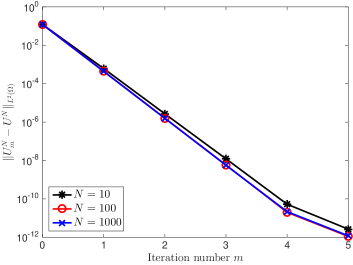
(a) $\kappa=0.5$, influence of $\tau=T/N$

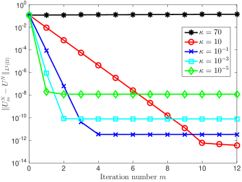
(b) $\tau=T/200$, influence of $\kappa$

Fig. 1: PinT BDF3 for Example 4.1: $T=0.5$ and $h=1/1000$.

4.2 Numerical results for subdiffusion

In this subsection, we test the performance of the algorithm for the subdiffusion problem in both 1D and 2D:

$$\left\{\begin{aligned} \partial_{t}^{\alpha}u-\Delta u&=f(x,t),&&\mbox{in}\,\,\,\Omega\times(0,T],\\ u&=0,&&\mbox{on}\,\,\,\partial\Omega\times(0,T],\\ u(0)&=v,&&\mbox{in}\,\,\,\Omega.\end{aligned}\right.$$ (46)

Example 4.2 (1D subdiffusion equation).

In the one-dimensional problem, the computational domain is $\Omega=(0,1)$ with equally spaced mesh. The mesh size is set to be $h=1/M$ with $M=1000$. We consider the following problem data

$$v=\delta_{1/2}(x)\quad\text{and}\quad f(x,t)=0.$$

Here the initial data is the Dirac-delta measure concentrated at $x=\frac{1}{2}$, which only belongs to $H^{-\frac{1}{2}-\epsilon}(\Omega)$ for any $\epsilon>0$. In the computation, the initial value is set to be the $L^{2}-$projection of delta function; see some details in [28].

Even though the initial condition is very weak, the inverse inequality and the analysis in [28, 29] implies the error estimate

$$\|U_{n}-u(t_{n})\|\leq c(\tau^{k}h^{-\frac{1}{2}-\epsilon}t_{n}^{-k}+h^{\frac{3}{2}-\epsilon}t_{n}^{-\alpha}),$$

and also the following convergence result

$$\|U_{n}-U_{n}^{m}\|\leq ct_{n}^{\alpha-1}h^{-\frac{1}{2}-\epsilon}\gamma(\kappa)^{m}$$

with the same $\gamma(\kappa)$ defined in (43).

Similar to the normal diffusion, the performance of all the PinT BDF$k$ ($k\leq 6$) have the same convergence profile, see Table 3. Moreover, we check the influence of different $N$ (or $\tau$) and $\kappa$ by using the PinT BDF3 scheme. Our theoretical result (43) indicates that the convergence factor is

$$\gamma(\kappa)=\frac{c\kappa\log(N)}{1-c\kappa\log(N)},$$

with some generic constant $c>1$. So we expect that the iteration converges linearly when $c\kappa\log(N)\in(0,1/2)$, i.e., $\kappa<1/(2c\log N)$. Besides, it implies that the convergence rate might deteriorate slightly for a large $N$ and a fixed $\kappa$. Surprisingly, our numerical results indicate that the iteration converges robustly even for relatively large $\kappa$ (cf. Figure 2b), and the step number $N$ seems not affect the convergence rate (cf. Figure 2a). From Figure 2b, we observe that the influence of $\kappa$ is similar to the normal diffusion case: the smaller $\kappa$ will lead to faster convergence rate but worse roundoff error. In practice, the choice $\kappa\approx 10^{-1}$ leads to an acceptable roundoff error ($\approx 10^{-11}$), and meanwhile the convergence is fast.

Table 3: Example 4.2: $e^{N}_{m}$ for $T=0.1$, $\alpha=0.5$, $\tau=T/100$, $h=1/1000$ and $\kappa=0.1$.

$m\backslash$ BDF$k$	$k=1$	$k=2$	$k=3$	$k=4$	$k=5$	$k=6$
0	2.46e-01	2.46e-01	2.46e-01	2.46e-01	2.46e-01	2.46e-01
1	6.31e-04	6.28e-04	6.28e-04	6.28e-04	6.28e-04	6.28e-04
2	2.88e-06	2.85e-06	2.85e-06	2.84e-06	2.85e-06	2.85e-06
3	1.34e-08	1.32e-08	1.32e-08	1.32e-08	1.33e-08	1.31e-08
4	8.12e-11	4.79e-11	4.98e-11	8.31e-11	4.27e-11	1.37e-10
5	1.88e-11	8.47e-12	1.86e-11	1.61e-11	3.44e-11	1.50e-10

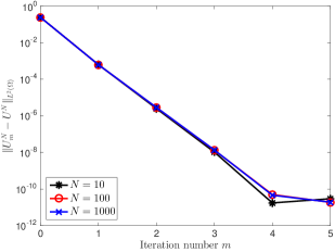
(a) $\kappa=0.1$, influence of $\tau=T/N$

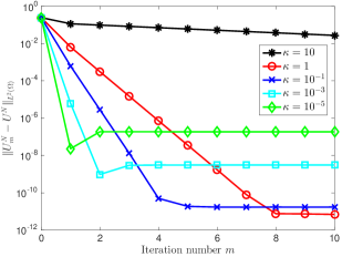
(b) $\tau=T/100$, influence of $\kappa$

Fig. 2: PinT BDF3 for Example 4.2: $\alpha=0.5$, $T=0.1$ and $h=1/1000$.

Example 4.3 (2D subdiffusion equation).

In this example, the spatial discretization is taken on the uniform triangulation of $\Omega=(0,1)^{2}$. We consider the following problem data

$$v(x)=\chi_{(0,\frac{1}{2})\times(0,\frac{1}{2})}(x)\quad\text{and}\quad f(x,t)=\cos(t)\chi_{(\frac{1}{2},1)\times(\frac{1}{2},1)}(x).$$

The numerical solutions are computed on a uniform triangular mesh with $h=10^{-2}$. We also observe that $\kappa$ needs to be properly chosen to balance the convergence rate and roundoff error, see Figure 3.

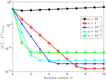
Fig. 3: PinT BDF3 for Example 4.3: convergence histories for $\alpha=0.5$, $\tau=10^{-3}$ and $h=10^{-2}$.

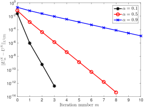
(a) $T=0.01$, influence of $\alpha$

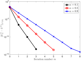
(b) $T=0.1$, influence of $\alpha$

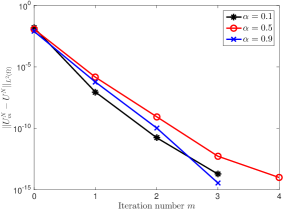
(c) $T=1$, influence of $\alpha$

Fig. 4: PinT BDF3 for Example 4.3: $\kappa=1/\log(N)$, $\tau=10^{-3}$ and $h=10^{-2}$.

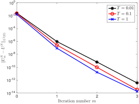
(a) $\alpha=0.1$, influence of $T$

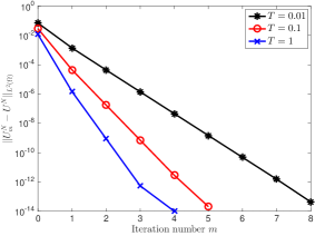
(b) $\alpha=0.5$, influence of $T$

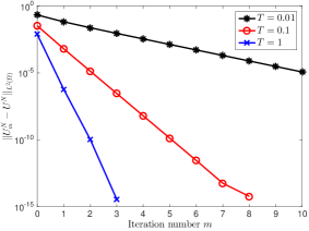
(c) $\alpha=0.9$, influence of $T$

Fig. 5: PinT BDF3 for Example 4.3: Influence of $T$ for the convergence rate, $\kappa=1/\log(N)$, $\tau=10^{-3}$ and $h=10^{-2}$.

Recall that, in the analysis, there is a generic constant $c$ in the convergence rate (43), which depends on the fractional order $\alpha$ and $T$. We numerically check these dependences and present the results in Figure 4 and 5, respectively. Taking $\kappa=1/\log(N)$, we observe the faster convergence rate with smaller $\alpha$ when $T$ is small, see Figure 4a. With the increase of $T$, these difference is getting smaller. Further, we observe the faster convergence rate with greater $T$ for various $\alpha$ in Figure 5, which shows the significant advantage of the proposed method for long-time simulation.

4.3 Extension to nonlinear problems

In this part, we shall briefly discuss a possible application of the time-parallel algorithm to the semilinear (sub)diffusion problem (with $\alpha\in(0,1]$):

$$\left\{\begin{aligned} \partial_{t}^{\alpha}u(t)+Au(t)+g(u(t))&=f(t),\quad\text{for all}~{}~{}t\in(0,T],\\ u(0)&=v.\end{aligned}\right.$$ (47)

To numerically solve (47), we follow the similar idea introduced in Section 3 and consider the modified CQ-BDF$k$ scheme:

$$\bar{\partial}_{\tau}^{\alpha}U^{n}-\Delta U^{n}+g(U^{n}) =\bar{f}_{n},\quad 1\leq n\leq N,$$ (48)

$$U^{n} =v,\quad n\leq 0,$$

where $\bar{f}_{n}:=f(x,t_{n})+a_{n}^{(k)}(f(x,0)+\Delta v-g(v))+\sum_{\ell=1}^{k-2}b_{\ell,n}^{(k)}\tau^{\ell}\partial_{t}^{\ell}f(x,0)$. If $\alpha=1$, it reduces to a modified BDF$k$ scheme for the classical semilinear parabolic equations. It was proved in [57, Theorem 3.4] that

$$\|U^{n}-u(t_{n})\|_{H}\leq c_{T}t_{n}^{\alpha-\min(k,1+2\alpha-\epsilon)}\tau^{\min(k,1+2\alpha-\epsilon)}.$$ (49)

for arbitrarily small $\epsilon$.

In order to solve the numerical solution in a time-parallel manner, we consider a modified Newton’s iteration to linearize the problem: for integer $\ell\geq 1$, we compute $U_{\ell}^{n}=U_{\ell-1}^{n}+W_{\ell}^{n}$ where $W_{\ell}^{n}$ satisfies homogeneous Dirichlet boundary condition and

$$(\bar{\partial}_{\tau}^{\alpha}-\Delta)W_{\ell}^{n}-g^{\prime}(\overline{U}_{\ell-1})W_{\ell}^{n} =\bar{f}_{n}-(\bar{\partial}_{\tau}^{\alpha}-\Delta)U_{\ell-1}^{n}-g(U_{\ell-1}^{n}),\quad 1\leq n\leq N,$$ (50)

$$W_{\ell}^{n} =0,\quad n\leq 0.$$

Here $\overline{U}_{\ell-1}$ denotes an average of $U_{\ell-1}^{n}$ in all levels, defined as

$$\overline{U}_{\ell-1}:=\frac{1}{N}\sum_{n=1}^{N}U_{\ell-1}^{n}.$$

Then, for each iteration, we shall solve the linear system (50) with a time-independent coefficient. Therefore, we can apply the strategy in Sections 2 and 3, i.e., applying waveform relaxation to derive an iterative solver: with $W_{\ell,0}^{n}=0$ and $m=1,2,\ldots$, for given $W_{\ell,m-1}^{n}$, we compute $W_{\ell,m}^{n}$ such that

$$(\bar{\partial}_{\tau}^{\alpha}-\Delta)W_{\ell,m}^{n}-g^{\prime}(\overline{U}_{\ell-1})W_{\ell,m}^{n} =\bar{f}_{n}-(\bar{\partial}_{\tau}^{\alpha}-\Delta)U_{\ell-1}^{n}-g(U_{\ell-1}^{n}),\quad n=1,2,\ldots,N,$$ (51)

$$W_{\ell,m}^{-n} =\kappa(W_{\ell,m}^{{N-n}}-W_{\ell,m-1}^{{N-n}}),\quad n=0,1,\ldots,N+1,$$

$$W_{\ell,m}^{n} =0,\quad n\leq-N.$$

This is a periodic-like system and hence it could be solved in parallel by diagonalization technique. We describe the complete iterative algorithm in Algorithm 3.

Algorithm 3   PinT BDF$k$ scheme for nonlinear models.

1:  Initialize $U_{0}^{n}=v$ for all $n\in\mathbb{Z}$, and set $\ell=0$.

2:  for $\ell=1,\ldots,L$ do

3:     Initialize $W_{\ell,0}^{n}=0$ for all $n\in\mathbb{Z}$, and set $m=0$.

4:     for $m=1,\ldots,m_{\ell}$ do

5:        Solve $W_{\ell,m}^{n}$ satisfying (51) in a time parallel manner using Algorithm 1 or 2.

6:        Check the stopping criterion of waveform relaxation.

7:     end for

8:     Update $U_{\ell}^{n}=U_{\ell-1}^{n}+W_{\ell,m}^{n}.$

9:     Check the stopping criterion of Newton’s iteration.

10:  end for

Example 4.4 (Allen–Cahn equations).

Taking $A=-\Delta$, $H=L^{2}(\Omega)$, $V=H_{0}^{1}(\Omega)$ and $g(u)=\frac{1}{\varepsilon^{2}}(u^{3}-u)$ in (47), we obtain the nonlinear problem with $\alpha\in(0,1]$:

$$\left\{\begin{aligned} \partial_{t}^{\alpha}u-\Delta u+\frac{1}{\varepsilon^{2}}(u^{3}-u)&=f(x,t)&&\text{ in }\Omega\times(0,T),\\ u&=0&&\text{ on }\partial\Omega\times(0,T),\\ u(0)&=v&&\text{ in }\Omega.\end{aligned}\right.$$ (52)

In case that $\alpha=1$ and $f(x,t)=0$, the model is called Allen–Cahn equation, which is a popular phase-field model, introduced in [1] to describe the motion of anti-phase boundaries in crystalline solids. In the context, $u$ represents the concentration of one of the two metallic components of the alloy and the parameter $\varepsilon$ involved in the nonlinear term represents the interfacial width, which is small compared to the characteristic length of the laboratory scale; see also [2, 6, 63] for some applications and [9] for some discussion for fractional models with $\alpha\in(0,1)$.

We shall investigate the numerical performance of Algorithm 3 on the domain $\Omega=(0,1)$ with equally spaced mesh. The exterior force $f(x,t)$ is chosen such that the exact solution yields $u=\frac{t^{2}}{\Gamma(3)}\sin(2\pi x)$.

First of all, we test the nonlinear problem (52) with $\varepsilon=1$ (mild nonlinearity), and report the error of Newton’s iteration, i.e. $e^{N}_{\ell}=\|U_{\ell}^{N}-U^{N}\|_{L^{2}(\Omega)}.$ In the computation, we and chose the stopping criteria of inner iteration (waveform relaxation) as

$$\|W_{\ell,m}^{n}-W_{\ell,m-1}^{n}\|_{\infty}<1\times 10^{-12}\quad\text{for all}\quad\ell\in\mathbb{N}^{+}.$$

The numbers of inner iteration are listed in the bracket. Invoking the error estimate (49), we report the numerical results for $\alpha=0.25$ (with BDF$1$ and BDF$2$) and $\alpha=0.75$ (with BDF$1$, BDF$2$ and BDF$3$) in Table 4. Numerical results in Table 4 indicate that the inner iteration (waveform relaxation) converges robustly and quickly for the linearized system (50), and the modified Newton’s iteration converges fast for both cases ($\alpha=0.25$ and $\alpha=0.75$), so does the Algorithm 3.

Table 4: Example 4.4: $e^{N}_{\ell}$ with $T=0.4$, $\tau=T/100$, $h=1/1000$, $\kappa=0.1$, and $\varepsilon=1$.

$\ell\backslash$ BDF$k$	$k=1$	$k=2$
0	6.30e-02	6.30e-02
1	9.27e-06$(5)$	9.27e-06$(5)$
2	3.64e-09$(4)$	3.63e-09$(4)$
3	1.42e-12$(3)$	1.42e-12$(3)$

(a) $\alpha=0.25$

$\ell\backslash$ BDF$k$	$k=1$	$k=2$	$k=3$
0	5.94e-02	5.94e-02	5.94e-02
1	6.83e-06$(5)$	6.80e-06$(5)$	6.80e-06$(5)$
2	1.95e-09$(4)$	1.92e-09$(4)$	1.92e-09$(4)$
3	5.23e-13$(3)$	5.06e-13$(3)$	5.03e-13$(3)$

(b) $\alpha=0.75$

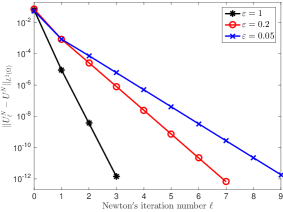
(a) $\alpha=0.25$

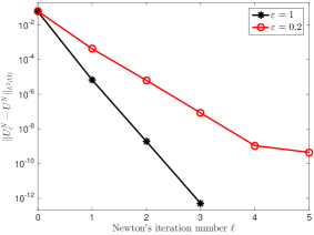
(b) $\alpha=0.75$

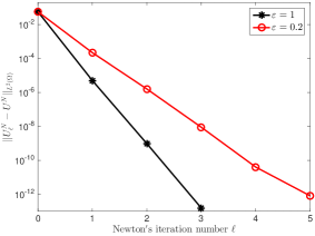
(c) $\alpha=1$

Fig. 6: PinT BDF3 for Example 4.4: Influence of the strength of nonlinearity.

Next, we investigate the influence of the strength of nonlinearity for both subdiffusion and normal diffusion cases in Figure 6. As can be seen from Table 4, the convergence behaviors of Algorithm 3 are insensitive with various BDF$k$ schemes, and hence the results of BDF2 scheme are presented. We observe that strong nonlinearity will lower the convergence rate, not only due to the strong nonlinearity itself to the Newton’s iteration, but also possibly to the more inaccurate average $\overline{U}_{\ell-1}$ in (50). As the nonlinearity getting stronger, for example $\varepsilon=0.05$ with $\alpha=0.75$ or $\alpha=1$, the modified Newton’s iteration does not converge. It is reasonable that the accuracy of average $\overline{U}_{\ell-1}$ hinges on the variation of the solutions on certain time interval. Practically, a windowing technique could be used in this algorithm: after a certain number of time steps computed in parallel in the current time window, the computation can be restarted for the next time window in a sequential way. This is beyond the scope of current paper and can be considered in the future.

References

- [1] S. M. Allen and J. W. Cahn. A microscopic theory for anti-phase boundary motion and its application to anti-phase domain coarsening. Acta Metall, 27:1085–1095, 1979.
- [2] D. M. Anderson, G. B. McFadden, and A. A. Wheeler. Diffuse-interface methods in fluid mechanics. Annual review of fluid mechanics, 30(1):139–165, 1998.
- [3] D. Baffet and J. S. Hesthaven. A kernel compression scheme for fractional differential equations. SIAM J. Numer. Anal., 55(2):496–520, 2017.
- [4] G. Bal. On the convergence and the stability of the parareal algorithm to solve partial differential equations. In Domain decomposition methods in science and engineering, volume 40 of Lect. Notes Comput. Sci. Eng., pages 425–432. Springer, Berlin, 2005.
- [5] L. Banjai and M. López-Fernández. Efficient high order algorithms for fractional integrals and fractional differential equations. Numer. Math., 141(2):289–317, 2019.
- [6] L.-Q. Chen. Phase-field models for microstructure evolution. Annual review of materials research, 32(1):113–140, 2002.
- [7] S. Chen, J. Shen, Z. Zhang, and Z. Zhou. A spectrally accurate approximation to subdiffusion equations using the log orthogonal functions. SIAM J. Sci. Comput., 42(2):A849–A877, 2020.
- [8] E. Cuesta, C. Lubich, and C. Palencia. Convolution quadrature time discretization of fractional diffusion-wave equations. Math. Comp., 75(254):673–696, 2006.
- [9] Q. Du, J. Yang, and Z. Zhou. Time-fractional Allen-Cahn equations: analysis and numerical methods. J. Sci. Comput., 85(2):Paper No. 42, 30, 2020.
- [10] M. Fischer. Fast and parallel Runge-Kutta approximation of fractional evolution equations. SIAM J. Sci. Comput., 41(2):A927–A947, 2019.
- [11] M. J. Gander. 50 years of time parallel time integration. In Multiple shooting and time domain decomposition methods, volume 9 of Contrib. Math. Comput. Sci., pages 69–113. Springer, Cham, 2015.
- [12] M. J. Gander, L. Halpern, J. Rannou, and J. Ryan. A direct time parallel solver by diagonalization for the wave equation. SIAM J. Sci. Comput., 41(1):A220–A245, 2019.
- [13] M. J. Gander, Y.-L. Jiang, B. Song, and H. Zhang. Analysis of two parareal algorithms for time-periodic problems. SIAM J. Sci. Comput., 35(5):A2393–A2415, 2013.
- [14] M. J. Gander, J. Liu, S.-L. Wu, X. Yue, and T. Zhou. Paradiag: Parallel-in-time algorithms based on the diagonalization technique. arXiv preprint, arXiv:2005.09158, 2020.
- [15] M. J. Gander and S. Vandewalle. Analysis of the parareal time-parallel time-integration method. SIAM J. Sci. Comput., 29(2):556–578, 2007.
- [16] M. J. Gander and S.-L. Wu. Convergence analysis of a periodic-like waveform relaxation method for initial-value problems via the diagonalization technique. Numer. Math., 143(2):489–527, 2019.
- [17] F. J. Gaspar and C. Rodrigo. Multigrid waveform relaxation for the time-fractional heat equation. SIAM J. Sci. Comput., 39(4):A1201–A1224, 2017.
- [18] A. Goddard and A. Wathen. A note on parallel preconditioning for all-at-once evolutionary PDEs. Electron. Trans. Numer. Anal., 51:135–150, 2019.
- [19] I. Golding and E. C. Cox. Physical nature of bacterial cytoplasm. Phys. Rev. Lett., 96:098102, Mar 2006.
- [20] G. H. Golub and C. F. Van Loan. Matrix computations. Johns Hopkins Studies in the Mathematical Sciences. Johns Hopkins University Press, Baltimore, MD, third edition, 1996.
- [21] X.-M. Gu and S.-L. Wu. A parallel-in-time iterative algorithm for volterra partial integro-differential problems with weakly singular kernel. Journal of Computational Physics, 417:109576, 2020.
- [22] W. Hackbusch. Parabolic multigrid methods. In Computing methods in applied sciences and engineering, VI (Versailles, 1983), pages 189–197. North-Holland, Amsterdam, 1984.
- [23] E. Hairer and G. Wanner. Solving Ordinary Differential Equations. II. Springer-Verlag, Berlin, second edition, 1996. Stiff and differential-algebraic problems.
- [24] G. Horton and S. Vandewalle. A space-time multigrid method for parabolic partial differential equations. SIAM J. Sci. Comput., 16(4):848–864, 1995.
- [25] D. Hou and C. Xu. A fractional spectral method with applications to some singular problems. Adv. Comput. Math., 43(5):911–944, 2017.
- [26] M. A. Inda and R. H. Bisseling. A simple and efficient parallel FFT algorithm using the BSP model. Parallel Comput., 27(14):1847–1878, 2001.
- [27] S. Jiang, J. Zhang, Q. Zhang, and Z. Zhang. Fast evaluation of the Caputo fractional derivative and its applications to fractional diffusion equations. Commun. Comput. Phys., 21(3):650–678, 2017.
- [28] B. Jin, R. Lazarov, J. Pasciak, and Z. Zhou. Galerkin FEM for fractional order parabolic equations with initial data in , . In Numerical analysis and its applications, volume 8236 of Lecture Notes in Comput. Sci., pages 24–37. Springer, Heidelberg, 2013.
- [29] B. Jin, B. Li, and Z. Zhou. Correction of high-order BDF convolution quadrature for fractional evolution equations. SIAM J. Sci. Comput., 39(6):A3129–A3152, 2017.
- [30] B. Jin and Z. Zhou. Incomplete iterative solution of the subdiffusion problem. Numer. Math., 145(3):693–725, 2020.
- [31] A. A. Kilbas, H. M. Srivastava, and J. J. Trujillo. Theory and Applications of Fractional Differential Equations. Elsevier Science B.V., Amsterdam, 2006.
- [32] J. W. Kirchner, X. Feng, and C. Neal. Fractal stream chemistry and its implications for contaminant transport in catchments. Nature, 403(6769):524–527, 2000.
- [33] N. Kopteva. Error analysis of the L1 method on graded and uniform meshes for a fractional-derivative problem in two and three dimensions. Math. Comp., 88(319):2135–2155, 2019.
- [34] H. Lee, J. Lee, and D. Sheen. Laplace transform method for parabolic problems with time-dependent coefficients. SIAM J. Numer. Anal., 51(1):112–125, 2013.
- [35] B. Li, K. Wang, and Z. Zhou. Long-time accurate symmetrized implicit-explicit BDF methods for a class of parabolic equations with non-self-adjoint operators. SIAM J. Numer. Anal., 58(1):189–210, 2020.
- [36] H.-l. Liao, D. Li, and J. Zhang. Sharp error estimate of the nonuniform L1 formula for linear reaction-subdiffusion equations. SIAM J. Numer. Anal., 56(2):1112–1133, 2018.
- [37] M. López-Fernández, C. Lubich, and A. Schädle. Adaptive, fast, and oblivious convolution in evolution equations with memory. SIAM J. Sci. Comput., 30(2):1015–1037, 2008.
- [38] C. Lubich. Discretized fractional calculus. SIAM J. Math. Anal., 17(3):704–719, 1986.
- [39] C. Lubich. Convolution quadrature and discretized operational calculus. I. Numer. Math., 52(2):129–145, 1988.
- [40] C. Lubich and A. Ostermann. Multigrid dynamic iteration for parabolic equations. BIT, 27(2):216–234, 1987.
- [41] C. Lubich, I. H. Sloan, and V. Thomée. Nonsmooth data error estimates for approximations of an evolution equation with a positive-type memory term. Math. Comp., 65(213):1–17, 1996.
- [42] Y. Maday and E. M. Rø nquist. Parallelization in time through tensor-product space-time solvers. C. R. Math. Acad. Sci. Paris, 346(1-2):113–118, 2008.
- [43] Y. Maday and G. Turinici. A parareal in time procedure for the control of partial differential equations. C. R. Math. Acad. Sci. Paris, 335(4):387–392, 2002.
- [44] W. McLean and K. Mustapha. Convergence analysis of a discontinuous Galerkin method for a sub-diffusion equation. Numer. Algorithms, 52(1):69–88, 2009.
- [45] W. McLean and K. Mustapha. Time-stepping error bounds for fractional diffusion problems with non-smooth initial data. J. Comput. Phys., 293:201–217, 2015.
- [46] W. McLean, I. H. Sloan, and V. Thomée. Time discretization via Laplace transformation of an integro-differential equation of parabolic type. Numer. Math., 102(3):497–522, 2006.
- [47] U. Miekkala and O. Nevanlinna. Convergence of dynamic iteration methods for initial value problem. SIAM J. Sci. Statist. Comput., 8(4):459–482, 1987.
- [48] K. Mustapha, B. Abdallah, and K. M. Furati. A discontinuous Petrov-Galerkin method for time-fractional diffusion equations. SIAM J. Numer. Anal., 52(5):2512–2529, 2014.
- [49] O. Nevanlinna. Remarks on Picard-Lindelöf iteration. I. BIT, 29(2):328–346, 1989.
- [50] R. R. Nigmatulin. The realization of the generalized transfer equation in a medium with fractal geometry. Phys. Stat. Sol. B, 133:425–430, 1986.
- [51] B. Ong and J. Schroder. Applications of time parallelization. Comput. Vis. Sci., page in press, 2020.
- [52] I. Podlubny. Fractional Differential Equations. Academic Press, Inc., San Diego, CA, 1999.
- [53] D. Sheen, I. H. Sloan, and V. Thomée. A parallel method for time-discretization of parabolic problems based on contour integral representation and quadrature. Math. Comp., 69(229):177–195, 2000.
- [54] M. Stynes, E. O’Riordan, and J. L. Gracia. Error analysis of a finite difference method on graded meshes for a time-fractional diffusion equation. SIAM J. Numer. Anal., 55(2):1057–1079, 2017.
- [55] V. Thomée. Galerkin Finite Element Methods for Parabolic Problems. Springer-Verlag, Berlin, second edition, 2006.
- [56] S. Vandewalle and R. Piessens. Efficient parallel algorithms for solving initial-boundary value and time-periodic parabolic partial differential equations. SIAM J. Sci. Statist. Comput., 13(6):1330–1346, 1992.
- [57] K. Wang and Z. Zhou. High-order time stepping schemes for semilinear subdiffusion equations. SIAM J. Numer. Anal., 58(6):3226–3250, 2020.
- [58] J. A. C. Weideman and L. N. Trefethen. Parabolic and hyperbolic contours for computing the Bromwich integral. Math. Comp., 76(259):1341–1356, 2007.
- [59] T. Weinzierl and T. Köppl. A geometric space-time multigrid algorithm for the heat equation. Numer. Math. Theory Methods Appl., 5(1):110–130, 2012.
- [60] S.-L. Wu and T. Zhou. Convergence analysis for three parareal solvers. SIAM J. Sci. Comput., 37(2):A970–A992, 2015.
- [61] Q. Xu, J. S. Hesthaven, and F. Chen. A parareal method for time-fractional differential equations. J. Comput. Phys., 293:173–183, 2015.
- [62] Y. Yan, M. Khan, and N. J. Ford. An analysis of the modified L1 scheme for time-fractional partial differential equations with nonsmooth data. SIAM J. Numer. Anal., 56(1):210–227, 2018.
- [63] P. Yue, J. J. Feng, C. Liu, and J. Shen. A diffuse-interface method for simulating two-phase flows of complex fluids. Journal of Fluid Mechanics, 515:293, 2004.
- [64] M. Zayernouri and G. E. Karniadakis. Fractional Sturm-Liouville eigen-problems: theory and numerical approximation. J. Comput. Phys., 252:495–517, 2013.
- [65] H. Zhu and C. Xu. A fast high order method for the time-fractional diffusion equation. SIAM J. Numer. Anal., 57(6):2829–2849, 2019.