A hierarchy in Majorana non-abelian tests and hidden variable models

Abstract

The recent progress of the Majorana experiments paves a way for the future tests of non-abelian braiding statistics and topologically-protected quantum information processing. However, a deficient design in those tests could be very dangerous and reach false-positive conclusions. A careful theoretical analysis is necessary in order to develop loophole-free tests. We introduce a series of classical hidden variable models to capture certain key properties of Majorana system: non-locality, topologically non-triviality, and quantum interference. Those models could help us to classify the Majorana properties and to set up the boundaries and limitations of Majorana non-abelian tests: fusion tests, braiding tests and test set with joint measurements. We find a hierarchy among those Majorana tests with increasing experimental complexity.

Introduction–The building blocks of topological quantum computation Kitaev (2003); Freedman et al. (2003); Nayak et al. (2008) are non-abelian anyons, which are proposed to show novel non-Abelian braiding statistics Leinaas and Myrheim (1977); Fredenhagen et al. (1989); Ivanov (2001); Nayak et al. (2008). A simple type of non-abelian anyon, i.e. Majorana zero mode (MZM), was theoretically proposed Read and Green (2000); Kitaev (2001); Fu and Kane (2008); Sato et al. (2009); Sau et al. (2010); Lutchyn et al. (2010); Oreg et al. (2010); Alicea (2010, 2012) in many physically realizable systems. Recent experimental progresses makes an almost conclusive observation of Majorana resonanceMourik et al. (2012); Deng et al. (2012); Churchill et al. (2013); Finck et al. (2013); Nadj-Perge et al. (2014); Albrecht et al. (2016); Deng et al. (2016); Zhang et al. (2017); Sun et al. (2016); Wang et al. (2018); Machida et al. (2019); Liu et al. (2018); Fornieri et al. (2019); Ren et al. (2019). Even though it is necessary to build up Majorana devices step-by-step Zhang et al. (2019) experimentally, these progresses makes a promising platform towards the test of non-abelian braiding statistics and the actual quantum information processing. The most popular schemes proposed for validating non-abelian statistics are braiding tests and fusion tests Nayak et al. (2008); Aasen et al. (2016); Clarke et al. (2011); Van Heck et al. (2012). Besides, joint-measurement, C-NOT gate, non-trivial T-gate test and Bell non-locality test  Bell (1966); Clauser et al. (1969) are believed to be necessary for quantum information processing. Here, we focus on relatively simple properties: Majorana non-local behaviors, topologically non-triviality, and quantum interference and entanglement in the near future.

In the hidden variable theories, the probabilities appeared when we measure physical quantities are due to the lack of the knowledge or statistical approximation in the underlying complex deterministic theoryBohm (1952); Everett (1957); Aspect et al. (1982a); Gisin (1991); Mermin (1993); Bassi and Ghirardi (2003); Aaronson (2005); Genovese (2005); Leggett (2006); Spekkens (2007); Augusiak et al. (2014), which reproduces certain behaviors in quantum mechanics. The experimental activities in the Bell inequality test eventually rule out local hidden variable explanations in several physical systems Aspect et al. (1982b); Weihs et al. (1998); Simon and Irvine (2003); García-Patrón et al. (2004); Colbeck and Renner (2011); Dada et al. (2011); Pusey et al. (2012); Hensen et al. (2015, 2016); Rosenfeld et al. (2017). But, this is not sufficient to say that the behaviors observed in other systems, e.g. Majorana platforms, are quantum mechanical. For our purpose, if we want to validate Majorana behaviors seriously for future quantum information applications, it is reasonable to treat the system as a black-box and perform the test subsequently. In that sense, potential hidden variable theories need to be carefully considered and excluded. Otherwise, a deficient test design might reach a positive but incorrect conclusion. For example, braiding and measurements in Majorana systems can generate topologically protected Clifford gates including entanglement gates, which can also be realized in certain hidden variable theories Spekkens (2007). Therefore, it is natural to ask whether we can find certain hidden variable theories such that each theory can capture certain properties of Majorana systems but can not capture other tests’ results; and the hope is to set up the limitations and boundaries of each Majorana test by using these theories.

In this work, we proposed a couple of classical hidden variable (HV) models, which are designed to capture and/or distinguish certain key quantum mechanical properties of Majorana systems: simplest Majorana non-local behaviors, topologically non-triviality and quantum interference. We want to show what properties can be seen in a particular test; and examine if the test results can be captured by both theories, which help us to set up the boundaries and limitations of the corresponding test. Based on this philosophy, we show:1) fusion tests only capture certain Majorana non-local behaviors but cannot capture others; 2) braiding tests show non-abelian statistics indicating topologically non-triviality, but not necessarily quantum interference; 3) test set with joint measurements are helpful and necessary to capture quantum interference in Majorana systems. Finally, we conclude that there exists a hierarchy among the Majorana non-abelian tests: Fusion test, braiding test, and test set with joint measurements.

Theoretical Framework– Now, we introduce a couple of HV models which are inspired from Spekkens’ famous model Spekkens (2007).

Classical HV theory I: We assume that (1) we have incomplete knowledge about the system states for some unknown complexity, (2) we get an outcome and observe incomplete knowledge after specific operations called measurements, (3) we cannot get access to their hidden complexity.

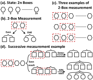
Figure 1: (a-c)The HV model I, where the number $1$ to $2n$ labels the position of boxes from left to right. (d) A four-box system (with total parity even) for fusion. If we get even parity result after Box 1,2-measurement, then continuing to apply Box 1,2-measurement, the state is unchanged. But if we apply a Box 2,3-measurement in the second step, we have two possible outcomes with equal probability.

a). State formalism–We consider a classical theory with a box representation, where each box corresponds to a MZM as shown in Fig.1; and the box can be either filled or empty. We assume that we can only know the parity of any (pair of) two boxes after measurement. For example, we measure the combination of the first and the second boxes and then get the result even. We can only know that the two boxes are either both filled or empty, but cannot determine the exact state of each box. This uncertainty is due to the unobserved classical complexity corresponding to the hidden-variables.

b). Measurement–We show three kinds of 2-box measurements (Box 1,2, Box 2,3, and Box 1,3) in Fig.1:. Each measurement returns two-box parity: even or odd. We also assume the parity of the all-box system is fixed similar to the Majorana systems. After Box 1,2-measurement for example, we could either obtain an even-parity result $\overbrace{\square\square}$ with a pair of square-symbols or obtain an odd parity result $\overbrace{\Circle\Circle}$ with a pair of circle-symbols; we use a bracket to label post-measurement box-pair called "connections". Considering a four-box (with total parity even) example shown in Fig.1 (d), Box1,2-measurement will reach either an even-even state: $\overbrace{\square\square}\overbrace{\square\square}$, or an odd-odd state:$\overbrace{\Circle\Circle}\overbrace{\Circle\Circle}$ with equal probability. If we repeat the previous measurement, we will get the same result; if the measurement is different from the previous one, we will get an uncertain result.

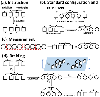
Figure 2: The HV model II. (a) Two equivalent form of state description: the lower means the back. (b) The standard configuration of a six-box state: the connection of Box1,6 is both the rightmost and frontmost as definition, and connection of Box3,5 is relative right and front to Box2,4. For non-standard configurations, we can apply crossover along with a parity change. (c) Both Box1,3 and Box2,4 measurements lead to standard configurations. (d) Braiding procedures $P^{2}_{23}$ and $P_{23}P_{32}$ . The braiding is confined in the plane perpendicular to the paper, or in the light-blue plane shown in the bracket.

Classical HV theory II: To include topology, we take into account the relative positions of connections if two connections have overlaps as shown in Fig.2 (a): (1) the front-back order (front connections are on the top of back ones) of the connections has a non-trivial consequence; (2) we also define the right-left order of connections, where the connection is the right as long as one box in the pair is in the right of all boxes in other box-pairs.

a). Standard states–For the order of connections discussed above, we can choose any order. However, for the convenience of discussion, we define a standard configuration with fixed order: the right connection is the front connection (e.g. in the upper part of Fig.2 (b)). For non-standard cases, we need to apply crossovers (exchange positions of two overlapping connections) to reach a standard configuration. Each crossover will induce a parity change (an example shown in Fig.2 (b)). In the text, we sometimes use an up-down bracket to describe an equivalent front-back position, e.g. in Fig.2 (a).

b). Measurement–We only consider measurements in standard configurations, i.e. "standard measurement rule". For an unidentified state, measurements (e.g. both Box2,4 and Box1,3 measurements in Fig.2 (c)) always result in standard configurations. On the other hand, if we know the connections of boxes, we only apply the standard rule for the standard cases. If we’re in a non-standard form, we need to apply crossovers to reach a standard one.

c). Braiding–In our theory, braiding corresponds to the position exchange of boxes in the plane shown in Fig.2 (d). Considering different directions of braiding, the exchange of Box $n_{1}$ and Box $n_{2}$ is labeled by $P_{n_{1}n_{2}}$ for anticlockwise exchange if $n_{1}<n_{2}$ (for clockwise exchange if $n_{1}>n_{2}$). In an example in Fig.2 (d), we apply two paths of braiding operations on the same initial state $\overbrace{\square\square}\overbrace{\square\square}$. The first path contains two successive $P_{23}$ where the first $P_{23}$ takes the state to a non-standard form and we apply a crossover to reach the standard one, then applying the second $P_{23}$ to get $\overbrace{\Circle\Circle}\overbrace{\Circle\Circle}$. In the second path, the first part is the same while we apply $P_{32}$ in the next step and we get a non-standard form with a knot. To reach a standard configuration, we apply a crossover to remove the knot and obtain the form $\overbrace{\square\square}\overbrace{\square\square}$.

Majorana non-Abelian Tests–Let us now consider a variety of Majorana tests, and check if their key properties, e.g. Majorana non-local behaviors, topologically non-triviality, and quantum interference, can be captured by our classical HV theory I and II.

A). Fusion test: Non-abelian anyon system follow special fusion processes which describe the outcomes after anyon combinations Nayak et al. (2008). Majorana zero modes belong to the Ising non-abelian anyon model, which includes three types of anyons: the vacuum $I$, non-abelian anyon $\sigma$ (i.e. Majorana), and the fermion $\psi$. A pair of $\sigma$ combine to fuse into either a vacuum or a fermion: $\sigma\times\sigma\rightarrow I+\psi$. With more anyons, we have multiple ways to fuse them together, where the quantum states describing fusion transformation can be written as:

$$|a,b\rightarrow i\rangle|i,c\rightarrow d\rangle=\sum_{j}(F^{d}_{abc})^{i}_{j}|b,c\rightarrow j\rangle|a,j\rightarrow d\rangle,$$ (1)

where $|a,b\rightarrow i\rangle|i,c\rightarrow d\rangle$ indicates a state with particular fusion channel where anyons $a$ and $b$ first fuse to $i$, and then $i$ and $c$ fuse to $d$. The matrix $(F^{d}_{abc})^{i}_{j}$ describes the transformation under different fusion channels, For Ising anyons, $F^{\sigma}_{\sigma\sigma\sigma}=\frac{1}{\sqrt{2}}\left(\begin{array}[]{cc}1&1\\ 1&-1\\ \end{array}\right).$

Now, let’s first focus on our HV theory I, we have:

$$\hexagon\hexagon\hexagon\hexagon\rightarrow\overbrace{\square\square}\overbrace{\square\square}\rightarrow(\overbrace{\square\overbrace{\square\square}\square}+\overbrace{\Circle\overbrace{\Circle\Circle}\Circle})/2$$ (2)

$$\hexagon\hexagon\hexagon\hexagon\rightarrow\overbrace{\Circle\Circle}\overbrace{\Circle\Circle}\rightarrow(\overbrace{\square\overbrace{\square\square}\square}+\overbrace{\Circle\overbrace{\Circle\Circle}\Circle})/2$$ (3)

Here, the first arrow in both Eq. (2) and (3) indicates the fusion (measurement) of Box$1,2$, which yields either fixed even parity (vacuum $I$) or odd parity (fermion $\psi$); the following Box2,3 measurement (second arrow) can have two possibilities: Box$2$ and Box$3$ first fuse into even parity or odd parity. We see that the measurements in HV model are analogous to the fusion, and reach the same measurement statistics as those in Ising anyon model described by the F-matrix above. Considering a proposed fusion test in Aasen et al. (2016), the topological superconducting device can realize two different 4-MZM fusion routes: 1) first create two pairs of MZMs and then fuse in the same pair as their creation, 2) first create two pairs of MZMs and then fuse in the different pairs. These two fusion routes gives different measurement statistics. As shown in Fig.3, it is simple to check that the corresponding fusion procedures in our HV model generate the same measurement outcome statistics as those in Majorana cases. Our HV model can fully capture the measurement outcome after fusion-only processes in Majorana systems (see part I of SI sup for more examples). This HV theory I does not include any topological consideration. Therefore, there is no doubt that the fusion tests can only capture certain Majorana non-locality behaviors but not including topological non-triviality.

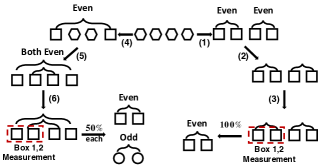
Figure 3: Fusion process of our HV model reproducing the Majorana fusion processes in Aasen et al. (2016). In the right path steps (1-3): the 4-box state splits into two pairs , both 2-box measurements obtain even, and then the measurement in the same box-pair Box1,2 obtains deterministic even parity result. In the left path steps (4-6): the 4-box state splits into two different pairs (Box1,4 and Box2,3) with even parity after measurement, and then the Box1,2 measurement gives us an equal probability of even or odd result.

B.) Braiding and topology: Non-Abelian anyons show nontrivial behaviors under the braiding process, and the exchange operation of anyons $a$ and $b$ can be captured by the operator $B_{ab}$, where these braiding operations can be written as $B_{ij}\propto 1+\gamma_{i}\gamma_{j}$ for Majorana modes Nayak et al. (2008).

Let us consider whether our HV theory I can capture braiding relations. For an example, braiding Box2,3 of initial state $\overbrace{\square\square}\overbrace{\square\square}$ requires the exchange of boxes in different box-pairs, as in different fusion channel of Majorana theory. After this braiding, we get $\hbox to0.0pt{$\overbrace{\phantom{\square\square\square}}$\hss}\square\overbrace{\square\square\square}$ (no connection order is considered here), then the Box1,3 measurement (correspondence to $\sigma_{y}$ measurement in quantum case sup ) results in even parity. However, the $\sigma_{y}$ measurement of quantum state $B_{23}|0\rangle$ reaches odd. Therefor we fail to capture the braiding process without topological consideration. Now let’s look at HV theory II. Considering the the same process on the initial state $\overbrace{\square\square}\overbrace{\square\square}$, we reach the state $\overbrace{\Circle\Circle}\overbrace{\Circle\Circle}$ as shown in the first path in Fig.2 (d), which is the same as quantum case.

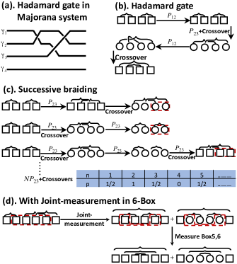
Figure 4: (a). Hadamard gate in majorana-based quantum computation. (b). Hadamard gate in our HV theory II wherein the second step and last step we have applied crossovers to change into a standard configuration. (c). Example of non-abelian braiding in four boxes case in our HV theory II. Suppose in the initial state Box3,4 are in even parity. The table shows the possibility $p$ to obtain the odd parity in Box3,4 measurement, where the label $n$ describes the number of successive braiding procedures of Box2 and Box3.

We further examine the Hadamard gates which can be realized using a sequence of Majorana braidings $H=B_{12}B_{23}B_{12}$ in the quantum anyon model as shown in Fig.4 (a). For our HV theory II in Fig.4 (b), we also successively braid Box1,2($P_{12}$), Box2,3($P_{23}$) and Box1,2($P_{12}$) and then apply a crossover to get a standard form, and then we can simply show any measurement here gives the same results as those in Majorana Hadamard gate. For the complete cases please refer to part II of SI sup .

Let’s consider the "successive braiding", i.e. a non-abelian braiding test Hyart et al. (2013) with four Majorana modes $\gamma_{1},\gamma_{2},\gamma_{3},\gamma_{4}$ where both $\gamma_{1},\gamma_{2}$ and $\gamma_{3},\gamma_{4}$ pair are initialized in even parity. We apply multiple braiding procedures ($n$ times) of $\gamma_{2}$ and $\gamma_{3}$ in an anti-clockwise way. We focus on the probability to obtain the odd result in the $(\gamma_{3}\gamma_{4})$ parity measurement at different $n$s. Braiding once, the parity of $\gamma_{3},\gamma_{4}$ has $50\%$ chance to be odd in measurement. After two successive braidings, we get the definite odd parity; after three successive braidings, we will get an equal probability of both results; after four successive braidings, we get the definite even parity. As the number $n$ increases, the probability will repeat this pattern with period 4. In our HV theory II, as shown in Fig.4 (c), we get the same measurement consequence as those in quantum case.

In either Majorana model or our HV theory II, the objects (MZMs or boxes) describing a specific fusion channel are all paired. Therefore, the braiding of two objects involves at most two pairs that is four MZMs or boxes. Considering the braiding of two boxes among $2n$ boxes, this procedure only changes the topology of two connections (of two box-pairs) involved in the braiding, but can not change the relative positions between these two connections and the other $n$-2 connections. Therefore, any single braiding step in more box-cases involves only four relevant boxes. Examples for braiding in more-MZM systems can be found in part II of SI sup . In summary, the braidings can be well described in our HV theory II with topology considerations; and this theory goes beyond the fusion tests and show the unique topological-nontrivial property of braiding operations.

C.) Joint-measurement and quantum interference: Let us assume there are two Majorana qubits, where each one is encoded into four MZMs; and the single-qubit Pauli measurements can be realized by fermion-parity measurement of different Majorana pairs within each qubit Nayak et al. (2008). The joint-measurement can be realized by the fermion-parity measurement of four MZMs, in which two MZMs are from one qubit and the other two are from the other qubit Nayak et al. (2008). For joint-measurement $ZZ$, the state $\frac{|0\rangle+|1\rangle}{\sqrt{2}}\otimes\frac{|0\rangle+|1\rangle}{\sqrt{2}}$ will collapses onto $(|00\rangle+|11\rangle)/\sqrt{2}$ if the measurement outcome is even, and thus generate entanglement between the two qubits. In our HV theory II with two "qubits" (eight boxes), we can measure the four-box joint-parity, in which two boxes are from the first qubit and the other two are from the second qubit. For example, if the Box1,4 and Box2,3 are initially even for both qubits, the joint-parity measurement of Box1,2 in the first qubit and Box1,2 in the second qubit gives the following projection:

$$\overbrace{\square\overbrace{\square\square}\square}|\overbrace{\square\overbrace{\square\square}\square}\rightarrow\\ \overbrace{\square\square}\overbrace{\square\square}|\overbrace{\square\square}\overbrace{\square\square}+\overbrace{\Circle\Circle}\overbrace{\Circle\Circle}|\overbrace{\Circle\Circle}\overbrace{\Circle\Circle}.$$ (4)

where we assume the measurement outcome is even, and the plus sign indicates two classical uncertain states with equal probability. This is an analog to joint-measurement $ZZ$ in the quantum theory.

Meanwhile, for another example with 6 MZMs in the initial state $|0_{12}0_{35}0_{46}\rangle$, we first joint-measure MZM $\gamma_{2}\gamma_{3}\gamma_{4}\gamma_{5}$ and assume even result, we get $(|0_{16}0_{23}0_{45}\rangle+|0_{16}1_{23}1_{45}\rangle)/\sqrt{2}$. Then the measurement of MZM $\gamma_{2}\gamma_{5}$ will reach a definite even result $|0_{16}0_{25}0_{34}\rangle$ due to the cancellation of quantum interference. However, as shown in Fig.4 (d), the HV theory II fails to capture this process and reaches $(\overbrace{\square\overbrace{\square\square}\overbrace{\square\square}\square}+\overbrace{\square\overbrace{\Circle\Circle}\overbrace{\Circle\Circle}\square})/2$ . We can look at another example in Majorana system–the CNOT gate of two MZM qubit which involve both joint-measurement and two-box measurement. We show in the part III of SIsup that our HV theory II can not capture CNOT gate process. It is clear that any HV theory can not capture the complete signature of quantum interference. Therefore, we conclude, to reveal certain signatures of quantum interference, the combination of joint-measurement and two box measurement are helpful and necessary.

Discussions– There are some other tests for more properties of Majorana systems. 1). Braiding and measurement only cannot generate T-gate, which however can be generated by preparing a noisy magic state ancilla along with state distillationBravyi and Kitaev (2005). T-gate test along with other Clifford operations specifies quantum property which could generate arbitrary quantum states. 2). Bell nonlocality tests clearly complete the Majorana system validation but require a fully universal quantum gate-set including T-gate to break Bell bound. However, the braiding and measurement only cannot break the Bell bound Deng and Duan (2013); Clarke et al. (2016); Romito and Gefen (2017). In the future, we need either to fabricate more sophisticated devices along with complicated experimental procedures or to propose novel and simple test schemes.

Acknowledgements

The authors acknowledge the support from NSF-China (Grant No.11974198) and the support from Beijing Academy of Quantum Information Sciences. D.E.L. also acknowledges the support from Thousand- Young-Talent program of China.

See pages 1 of supl5.pdf See pages 2 of supl5.pdf See pages 3 of supl5.pdf See pages 4 of supl5.pdf See pages 5 of supl5.pdf

References

- Kitaev (2003) A. Y. Kitaev, Annals of Physics 303, 2 (2003).
- Freedman et al. (2003) M. Freedman, A. Kitaev, M. Larsen, and Z. Wang, Bulletin of the American Mathematical Society 40, 31 (2003).
- Nayak et al. (2008) C. Nayak, S. H. Simon, A. Stern, M. Freedman, and S. Das Sarma, Rev. Mod. Phys. 80, 1083 (2008).
- Leinaas and Myrheim (1977) J. M. Leinaas and J. Myrheim, Il Nuovo Cimento B (1971-1996) 37, 1 (1977).
- Fredenhagen et al. (1989) K. Fredenhagen, K.-H. Rehren, and B. Schroer, Communications in Mathematical Physics 125, 201 (1989).
- Ivanov (2001) D. A. Ivanov, Phys. Rev. Lett. 86, 268 (2001).
- Read and Green (2000) N. Read and D. Green, Phys. Rev. B 61, 10267 (2000).
- Kitaev (2001) A. Y. Kitaev, Physics-Uspekhi 44, 131 (2001).
- Fu and Kane (2008) L. Fu and C. L. Kane, Phys. Rev. Lett. 100, 096407 (2008).
- Sato et al. (2009) M. Sato, Y. Takahashi, and S. Fujimoto, Phys. Rev. Lett. 103, 020401 (2009).
- Sau et al. (2010) J. D. Sau, R. M. Lutchyn, S. Tewari, and S. Das Sarma, Phys. Rev. Lett. 104, 040502 (2010).
- Lutchyn et al. (2010) R. M. Lutchyn, J. D. Sau, and S. Das Sarma, Phys. Rev. Lett. 105, 077001 (2010).
- Oreg et al. (2010) Y. Oreg, G. Refael, and F. von Oppen, Phys. Rev. Lett. 105, 177002 (2010).
- Alicea (2010) J. Alicea, Phys. Rev. B 81, 125318 (2010).
- Alicea (2012) J. Alicea, Reports on progress in physics 75, 076501 (2012).
- Mourik et al. (2012) V. Mourik, K. Zuo, S. M. Frolov, S. R. Plissard, E. P. A. M. Bakkers, and L. P. Kouwenhoven, Science 336, 1003 (2012).
- Deng et al. (2012) M. Deng, C. Yu, G. Huang, M. Larsson, P. Caroff, and H. Xu, Nano letters 12, 6414 (2012).
- Churchill et al. (2013) H. O. H. Churchill, V. Fatemi, K. Grove-Rasmussen, M. T. Deng, P. Caroff, H. Q. Xu, and C. M. Marcus, Phys. Rev. B 87, 241401 (2013).
- Finck et al. (2013) A. D. K. Finck, D. J. Van Harlingen, P. K. Mohseni, K. Jung, and X. Li, Phys. Rev. Lett. 110, 126406 (2013).
- Nadj-Perge et al. (2014) S. Nadj-Perge, I. K. Drozdov, J. Li, H. Chen, S. Jeon, J. Seo, A. H. MacDonald, B. A. Bernevig, and A. Yazdani, Science 346, 602 (2014).
- Albrecht et al. (2016) S. M. Albrecht, A. P. Higginbotham, M. Madsen, F. Kuemmeth, T. S. Jespersen, J. Nygård, P. Krogstrup, and C. Marcus, Nature 531, 206 (2016).
- Deng et al. (2016) M. Deng, S. Vaitiekėnas, E. B. Hansen, J. Danon, M. Leijnse, K. Flensberg, J. Nygård, P. Krogstrup, and C. M. Marcus, Science 354, 1557 (2016).
- Zhang et al. (2017) H. Zhang, Ö. Gül, S. Conesa-Boj, M. Nowak, M. Wimmer, K. Zuo, V. Mourik, F. K. de Vries, J. van Veen, M. W. A. de Moor, J. D. S. Bommer, D. J. van Woerkom, D. Car, S. R. Plissard, E. P. A. M. Bakkers, M. Quintero-Pérez, M. C. Cassidy, S. Koelling, S. Goswami, K. Watanabe, T. Taniguchi, and L. P. Kouwenhoven, Nature Communications 8, 16025 (2017).
- Sun et al. (2016) H.-H. Sun, K.-W. Zhang, L.-H. Hu, C. Li, G.-Y. Wang, H.-Y. Ma, Z.-A. Xu, C.-L. Gao, D.-D. Guan, Y.-Y. Li, C. Liu, D. Qian, Y. Zhou, L. Fu, S.-C. Li, F.-C. Zhang, and J.-F. Jia, Phys. Rev. Lett. 116, 257003 (2016).
- Wang et al. (2018) D. Wang, L. Kong, P. Fan, H. Chen, S. Zhu, W. Liu, L. Cao, Y. Sun, S. Du, J. Schneeloch, et al., Science 362, 333 (2018).
- Machida et al. (2019) T. Machida, Y. Sun, S. Pyon, S. Takeda, Y. Kohsaka, T. Hanaguri, T. Sasagawa, and T. Tamegai, Nature materials , 1 (2019).
- Liu et al. (2018) Q. Liu, C. Chen, T. Zhang, R. Peng, Y.-J. Yan, C.-H.-P. Wen, X. Lou, Y.-L. Huang, J.-P. Tian, X.-L. Dong, G.-W. Wang, W.-C. Bao, Q.-H. Wang, Z.-P. Yin, Z.-X. Zhao, and D.-L. Feng, Phys. Rev. X 8, 041056 (2018).
- Fornieri et al. (2019) A. Fornieri, A. M. Whiticar, F. Setiawan, E. Portolés, A. C. Drachmann, A. Keselman, S. Gronin, C. Thomas, T. Wang, R. Kallaher, et al., Nature 569, 89 (2019).
- Ren et al. (2019) H. Ren, F. Pientka, S. Hart, A. T. Pierce, M. Kosowsky, L. Lunczer, R. Schlereth, B. Scharf, E. M. Hankiewicz, L. W. Molenkamp, et al., Nature 569, 93 (2019).
- Zhang et al. (2019) H. Zhang, D. E. Liu, M. Wimmer, and L. P. Kouwenhoven, Nature Communications 10, 5128 (2019).
- Aasen et al. (2016) D. Aasen, M. Hell, R. V. Mishmash, A. Higginbotham, J. Danon, M. Leijnse, T. S. Jespersen, J. A. Folk, C. M. Marcus, K. Flensberg, and J. Alicea, Phys. Rev. X 6, 031016 (2016).
- Clarke et al. (2011) D. J. Clarke, J. D. Sau, and S. Tewari, Phys. Rev. B 84, 035120 (2011).
- Van Heck et al. (2012) B. Van Heck, A. Akhmerov, F. Hassler, M. Burrello, and C. Beenakker, New Journal of Physics 14, 035019 (2012).
- Bell (1966) J. S. Bell, Rev. Mod. Phys. 38, 447 (1966).
- Clauser et al. (1969) J. F. Clauser, M. A. Horne, A. Shimony, and R. A. Holt, Phys. Rev. Lett. 23, 880 (1969).
- Bohm (1952) D. Bohm, Phys. Rev. 85, 166 (1952).
- Everett (1957) H. Everett, Rev. Mod. Phys. 29, 454 (1957).
- Aspect et al. (1982a) A. Aspect, J. Dalibard, and G. Roger, Phys. Rev. Lett. 49, 1804 (1982a).
- Gisin (1991) N. Gisin, Physics Letters A 154, 201 (1991).
- Mermin (1993) N. D. Mermin, Rev. Mod. Phys. 65, 803 (1993).
- Bassi and Ghirardi (2003) A. Bassi and G. Ghirardi, Physics Reports 379, 257 (2003).
- Aaronson (2005) S. Aaronson, Phys. Rev. A 71, 032325 (2005).
- Genovese (2005) M. Genovese, Physics Reports 413, 319 (2005).
- Leggett (2006) A. J. Leggett, Foundations of Physics 33, 1469 (2006).
- Spekkens (2007) R. W. Spekkens, Phys. Rev. A 75, 032110 (2007).
- Augusiak et al. (2014) R. Augusiak, M. Demianowicz, and A. Acín, Journal of Physics A: Mathematical and Theoretical 47, 424002 (2014).
- Aspect et al. (1982b) A. Aspect, J. Dalibard, and G. Roger, Phys. Rev. Lett. 49, 1804 (1982b).
- Weihs et al. (1998) G. Weihs, T. Jennewein, C. Simon, H. Weinfurter, and A. Zeilinger, Phys. Rev. Lett. 81, 5039 (1998).
- Simon and Irvine (2003) C. Simon and W. T. Irvine, Physical review letters 91, 110405 (2003).
- García-Patrón et al. (2004) R. García-Patrón, J. Fiurášek, N. J. Cerf, J. Wenger, R. Tualle-Brouri, and P. Grangier, Physical review letters 93, 130409 (2004).
- Colbeck and Renner (2011) R. Colbeck and R. Renner, Nature communications 2, 1 (2011).
- Dada et al. (2011) A. C. Dada, J. Leach, G. S. Buller, M. J. Padgett, and E. Andersson, Nature Physics 7, 677 (2011).
- Pusey et al. (2012) M. F. Pusey, J. Barrett, and T. Rudolph, Nature Physics 8, 475 (2012).
- Hensen et al. (2015) B. Hensen, H. Bernien, A. E. Dréau, A. Reiserer, N. Kalb, M. S. Blok, J. Ruitenberg, R. F. Vermeulen, R. N. Schouten, C. Abellán, et al., Nature 526, 682 (2015).
- Hensen et al. (2016) B. Hensen, N. Kalb, M. Blok, A. Dréau, A. Reiserer, R. Vermeulen, R. Schouten, M. Markham, D. Twitchen, K. Goodenough, et al., Scientific reports 6, 30289 (2016).
- Rosenfeld et al. (2017) W. Rosenfeld, D. Burchardt, R. Garthoff, K. Redeker, N. Ortegel, M. Rau, and H. Weinfurter, Physical review letters 119, 010402 (2017).
- (57) See Supplemental information (SI) for more details.
- Hyart et al. (2013) T. Hyart, B. van Heck, I. C. Fulga, M. Burrello, A. R. Akhmerov, and C. W. J. Beenakker, Phys. Rev. B 88, 035121 (2013).
- Bravyi and Kitaev (2005) S. Bravyi and A. Kitaev, Phys. Rev. A 71, 022316 (2005).
- Deng and Duan (2013) D.-L. Deng and L.-M. Duan, Phys. Rev. A 88, 012323 (2013).
- Clarke et al. (2016) D. J. Clarke, J. D. Sau, and S. Das Sarma, Phys. Rev. X 6, 021005 (2016).
- Romito and Gefen (2017) A. Romito and Y. Gefen, Phys. Rev. Lett. 119, 157702 (2017).