An analysis of systematic effects in finite size scaling studies using the gradient flow

Alessandro Nada^a and Alberto Ramos^b

Abstract

  We propose a new strategy for the determination of the step scaling function $\sigma(u)$ in finite size scaling studies using the Gradient Flow. In this approach the determination of $\sigma(u)$ is broken in two pieces: a change of the flow time at fixed physical size, and a change of the size of the system at fixed flow time. Using both perturbative arguments and a set of simulations in the pure gauge theory we show that this approach leads to a better control over the continuum extrapolations. Following this new proposal we determine the running coupling at high energies in the pure gauge theory and re-examine the determination of the $\Lambda$-parameter, with special care on the perturbative truncation uncertainties.
 

1 Introduction

In recent years the gradient flow [1, 2] (GF) has found many successful applications. In particular, when combined with the ideas of finite-size scaling [3], it provides a powerful tool for the determination of the running coupling in asymptotically-free strongly-coupled gauge theories [4, 5, 6]. The applications include the determination of the strong coupling in QCD, and the study of near conformal systems (see [7] for a recent review).

Coupling definitions based on the gradient flow have some properties that make them very attractive. First, the relevant observables show a small variance. A modest numerical effort allows their determination with a sub-percent precision. Second, the gradient flow coupling is given directly as an expectation value. Its determination only involves the numerical integration of the flow equations, something that in practice can be done with arbitrary precision without having to perform any fits, or taking any limit. This means that finite-size scaling studies using the GF only have one source of systematic effect: the continuum extrapolation.

Nevertheless, it has been shown that these systematic effects are difficult to keep under control (see [8] for a review). It was soon noticed [9] that seemingly innocent extrapolations could cause large systematic effects. Although the same work suggested to simply use larger flow times as a way to have a better control of the continuum extrapolation, this comes with an increase in the variance of the observable. One of the strong points of GF studies, the high statistical precision, had to be sacrificed. Some efforts were made in order to understand the anatomy of these cutoff effects, first in a perturbative context to tree level [10], and later more systematically from an effective field theory point of view [11]. It became clear that the integration of the flow equations and the evaluation of the relevant observables at positive flow time could be performed in a way that no $\mathcal{O}(a^{2})$ effects are produced: it is enough to use classically improved discretizations [11]. Still, the use of these improved observables did not reduce substantially the observed scaling violations (see for example [12]). Unavoidably large lattices have to be simulated in GF studies, and the continuum extrapolation will remain the main source of concern.

In this work we study the main sources of systematic effects in finite-size scaling studies using the GF. We will argue that changes in the flow time $t$ are responsible for the scaling violations. On the contrary, when different finite volume couplings are determined at the same value of the flow time $t$, the scaling violations are very small. This observation will be supported by a non-perturbative study. Moreover it will allow us to propose a new strategy for the determination of the step scaling function by breaking it up into two pieces: first a change in the flow time, without any change in the volume, second a change in the volume without any change in the flow time. Since the first step can be performed without having to double the lattices, the continuum extrapolation can be performed much more accurately. We will discuss in detail the advantages of this approach. Finally we will apply this alternative strategy to the case of pure gauge ${\rm SU}(3)$. Using the same datasets of [13], we will revisit the most crucial part of this work: the running at high energies and the matching with the asymptotic perturbative regime.

We also include an analysis of the variance of flow observables, allowing us to predict the dependence of the statistical uncertainties with the flow time $t$.

2 The continuum extrapolation

2.1 Preliminaries

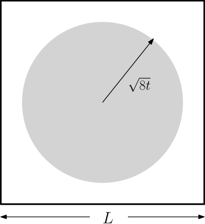
Figure 1: The GF coupling in finite volume $\bar{g}^{2}(\mu)$ is measured by computing the action density of the flow field $B_{\mu}(t,x)$ smeared over a distance $\sqrt{8t}=\mu^{-1}$ (see eq. (2.3)). The renormalization scale $\mu$ and the size of the system $L$ are linked by the relation $\sqrt{8t}=cL$ (with $c$ a constant).

The gradient flow provides a set of renormalized observables with small variance that are easy to compute via numerical simulations. The key idea consists in adding an extra time coordinate to the gauge field, the flow time $t$. The dependence of the gauge field $B_{\mu}(t,x)$ on the flow time is given by the first order diffusion equation

$$\partial_{t}B_{\mu}(t,x)=D_{\nu}G_{\nu\mu}(t,x)\,; \qquad B_{\mu}(0,x)=A_{\mu}(x)\,.$$ (2.1)

$$G_{\mu\nu}(t,x)=D_{\mu}B_{\nu}(t,x)-D_{\nu}B_{\mu}(t,x)\,; \qquad D_{\mu}=\partial_{\mu}+[B_{\mu},\cdot]\,.$$ (2.2)

The flow time has dimensions of length squared, and therefore introduces a scale into the problem (see figure 1). Gauge-invariant composite operators defined at positive flow time are automatically renormalized [14]. In particular, a renormalized coupling at scale $\mu=1/\sqrt{8t}$ can be defined by using the action density [2]

$$\bar{g}^{2}(\mu)\Big{|}_{\mu=1/\sqrt{8t}}\propto t^{2}\langle E(t,x)\rangle\,.\qquad\left(E(t,x)=G_{\mu\nu}^{a}(t,x)G_{\mu\nu}^{a}(t,x)\right)$$ (2.3)

In finite volume schemes where the invariance under Euclidean time translations is broken, like the Schrödinger Functional (SF) or open-SF boundary conditions, the coupling is only measured at the time-slice $x_{0}=T/2$ and usually only certain components of the field strength are used

$$E_{\rm m}(t,x) = G_{ij}^{a}(t,x)G_{ij}^{a}(t,x)\Big{|}_{x_{0}=T/2}\,,$$ (2.4a)

$$E_{\rm e}(t,x) = G_{0j}^{a}(t,x)G_{0j}^{a}(t,x)\Big{|}_{x_{0}=T/2}\,.$$ (2.4b)

The coupling defined using $E=E_{\rm m}$ is usually referred as magnetic and the one using $E=E_{\rm e}$ as electric.

Most applications of the gradient flow until today derive from these coupling definitions. In infinite volume the scale $\mu_{0}=1/\sqrt{8t_{0}}$ at which the coupling $\bar{g}^{2}(\mu_{0})$ takes some pre-defined value is used to define the reference scale $t_{0}$. In the context of finite-size scaling, the renormalization scale $\mu=1/\sqrt{8t}$ is linked with the linear size of the system

$$\mu^{-1}=\sqrt{8t}=cL\,,$$ (2.5)

and therefore the coupling “runs” with the size $L$ (see fig 1). The constant $c$ defines a scheme by fixing the ratio of the length of the system and the flow time scale $\sqrt{8t}$. The full definition of the GF coupling in finite volume reads

$$\bar{g}^{2}_{c}(\mu)=\mathcal{N}(c)\,t^{2}\langle E(t,x)\rangle\Big{|}_{\mu^{-1}=\sqrt{8t}=cL}\,.$$ (2.6)

The constant $\mathcal{N}(c)$ has been determined for different choices of boundary conditions [4, 5, 6, 15].

When computing the gradient flow coupling on the lattice there are several choices to make, beyond the action chosen for the simulation. First, the flow equation (2.1) has to be translated to the lattice. Second, there are many valid discretizations of the energy density $E(t,x)$. It is well understood that using the Zeuthen flow to integrate the flow equations and using any classically improved discretization of the action density $E(t,x)$ guarantees that no further $\mathcal{O}(a^{2})$ effects are generated. The only remaining $\mathcal{O}(a^{2})$ effects are those of the choice of action for the simulation and an additional counterterm, only affecting flow quantities [11].

On the lattice, where we can work only with dimensionless quantities, the finite volume gradient flow coupling (equation (2.6)) can be measured by determining $\bar{g}^{2}(\mu)$ at the flow time (in lattice units) $\sqrt{8t}/a=cL/a$. It is also common to use a lattice version of the normalization factor $\mathcal{N}(c,a/\sqrt{8t})$ instead of the $\mathcal{N}(c)$ of eq. (2.6), in order to ensure that the leading order perturbative relation

$$\bar{g}^{2}_{c}(\mu)\raisebox{-0.43057pt}{ $\stackrel{{\scriptstyle\small{\mu\to\infty}}}{{\sim}}$}\bar{g}^{2}_{\overline{\rm MS}}(\mu)+\mathcal{O}(\bar{g}^{4}_{\overline{\rm MS}})\,,$$ (2.7)

is exact for any lattice size.

The key character in finite-size scaling studies is the step scaling function

$$\sigma(u)=\bar{g}_{c}^{2}(\mu/2)\Big{|}_{\bar{g}_{c}^{2}(\mu)=u}\,.$$ (2.8)

It measures how much the coupling changes under a variation in the renormalization scale of a factor two. Its determination in lattice simulations is performed via a matching of the bare parameters. At a fixed value of the bare coupling $g_{0}^{2}$ (and therefore fixed value of the lattice spacing $a$), one determines the GF coupling on a lattice of size $L/a$ (resulting in $\bar{g}^{2}(\mu)$), and on a lattice $2L/a$ (resulting in $\bar{g}^{2}(\mu/2)$). This allows the determination of a lattice approximation of the step scaling function:

$$\Sigma(u,a/\sqrt{8t})=\bar{g}_{c}^{2}(\mu/2)\Big{|}_{\bar{g}_{c}^{2}(\mu)=u}\raisebox{-0.43057pt}{ $\stackrel{{\scriptstyle\small{a/\sqrt{8t}\to 0}}}{{\sim}}$}\sigma(u)\,.$$ (2.9)

In the rest of this section we will be concerned with the continuum extrapolation of $\Sigma(u,a/\sqrt{8t})$; before that however, let us insist on two points:

• The direct determination of $\Sigma$, as suggested above, requires the determination of the GF couplings at two different renormalization scales $\mu$ and $\mu/2$, on lattices of two different sizes $L/a$ and $2L/a$.

• It is clear that once $c$ (eq. (2.5)) is fixed, taking $a/L\to 0$ is equivalent to taking $a/\sqrt{8t}\to 0$, so the usual notation that uses $a/L$ as the variable to parametrize cutoff effects is fully justified. Nevertheless, it is $a/\sqrt{8t}=a\mu$ the natural variable to measures the size of cutoff effects. Note that for the typical choices of $c\in[0.2-0.5]$ we have scale $\sqrt{8t}<L$.

  With this choice of the renormalization scale, it is clear that, at fixed $L/a$, larger values of $c$ would lead to smaller cutoff effects. This notation will also be convenient for the discussion that follows.

2.2 A new strategy for the determination of $\sigma(u)$

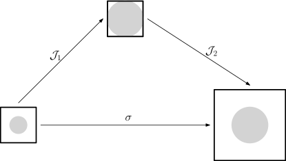
Figure 2: The determination of the step scaling function $\sigma$ involves a change in the renormalization scale and in the size of the system of a factor two. These two steps do not need to be performed at the sime time. The figure shows that $\sigma$ can be determined as the composition of the function $\mathcal{J}_{1}$ that changes the renormalization scale $\mu\to\mu/2$ at fixed size $L$, with the function $\mathcal{J}_{2}$ that changes the size $L\to 2L$ at fixed renormalization scale $\mu$.

As already pointed out, the determination of the lattice step scaling function involves two steps: a change in the renormalization scale by a factor two, and change in the lattice size by the same factor. In previous works these two changes have been performed at the same time in a single step, but conceptually there is no need to do so.

Figure 2 shows that the value of the step scaling function $\sigma(u)$ can be determined by the composition of two functions. First we have

$$\mathcal{J}_{1}(u)=\bar{g}^{2}_{2c}(\mu/2)\Big{|}_{\bar{g}^{2}_{c}(\mu)=u}\,.$$ (2.10)

This function changes the renormalization scale by a factor two $\mu\to\mu/2$ at fixed physical size $L$. Second, we need to determine

$$\mathcal{J}_{2}(u)=\bar{g}^{2}_{c}(\mu/2)\Big{|}_{\bar{g}^{2}_{2c}(\mu/2)=u}\,.$$ (2.11)

This function changes the lattice size $L\to 2L$ keeping constant the renormalization scale $\mu^{-1}=\sqrt{8t}$.

The relation

$$\sigma=\mathcal{J}_{2}\circ\mathcal{J}_{1}\,,$$ (2.12)

is now exact, and provides an alternative method to determine $\sigma$.

Our main assumption is that large scaling violations come with changes in the renormalization scale. We will later provide evidence that this is the case, but for the moment let us discuss why this opens up the possibility to improve the quality of the continuum extrapolations. Let us start by explaining how these functions are computed in practice:

• The determination of $\mathcal{J}_{1}$ involves measuring how much the coupling changes when the renormalization scale is varied as $\mu\to\mu/2$ at constant physical size $L$. This is simply achieved by measuring on a lattice simulation the value of the GF coupling at two different flow times (i.e. $t\to 4t$, see eq. (2.5)). Crucially, this determination does not require to double the lattice size, allowing precise results without the need of very large values of $L/a$.

• The determination of $\mathcal{J}_{2}$ requires to change the physical size $L$ without varying the renormalization scale. In practice one fixes the bare coupling $g_{0}^{2}$ at a given value, and then measures the GF coupling on a $L/a$ lattice at flow time $\sqrt{8t}/a=cL/a$ and on a $2L/a$ lattice at the same $t$. This step requires to change the lattice size, but since the renormalization scale remains the same, one expects reduced cutoff effects. In some sense the determination of $\mathcal{J}_{2}$ corresponds to measuring the finite volume effects in $\bar{g}^{2}_{c}(\mu)$ (see figure 2).

In the rest of this section we will provide evidence of these statements, but before that let us further comment on two points:

• The determination of the functions $\mathcal{J}_{1}$ and $\mathcal{J}_{2}$ can be done on the lattice just by applying the definitions equation (2.10) and (2.11). Note however that in this case the functions will carry a dependence on the cutoff. We will label these functions $\hat{\mathcal{J}}_{1}(u,a/\sqrt{8t})$ and $\hat{\mathcal{J}}_{2}(u,a/\sqrt{8t})$ respectively.

• In this work all numerical results make use of the same discretizations used in [13]. We encourage the reader to consult this reference for more details. Here it is enough to say that we define the GF coupling with SF boundary conditions and that our preferred setup, based on theoretical expectations, uses the Zeuthen flow and an improved definition of $E(t,x)$. This preferred setup will also be compared with the more common combination Wilson flow/Clover observable.

  Moreover, we will focus in the rest of the text on the magnetic definition of the GF coupling (see equations (2.4)). Of course, our discussion is general, and does not depend on these particular choices.

2.2.1 Leading order perturbation theory

As a first look at the proposal we examine the leading order perturbative relation. We use the continuum norm $\mathcal{N}(c)$ in the evaluation of the finite volume couplings $\bar{g}^{2}_{c}$ and examine, to leading order in perturbation theory, the quantities

$$\hat{\mathcal{C}_{0}}(a/\sqrt{8t})=\frac{\Sigma(u,a/\sqrt{8t})}{u}\,,\quad\hat{\mathcal{C}}_{1}(a/\sqrt{8t})=\frac{\hat{\mathcal{J}}_{1}(u,a/\sqrt{8t})}{u}\,,\quad\hat{\mathcal{C}}_{2}(a/\sqrt{8t})=\frac{\hat{\mathcal{J}}_{2}(u,a/\sqrt{8t})}{u}\,.$$ (2.13)

Note that since we are working at leading order in $\bar{g}^{2}$, and thanks to the normalization by the constant factor $u$, all these quantities are one in the continuum.

In this example we will examine a typical case where we consider data for

$$L/a=8,10,12,16,18,20,24,32,36,40,48\,.$$ (2.14)

We will use $c=0.2$ (see eq. (2.5)). Let us note a few basic points:

• The determination of $\hat{\mathcal{C}_{0}}(a/\sqrt{8t})$ and $\hat{\mathcal{C}_{2}}(a/\sqrt{8t})$ requires to double the lattice size. This means that with our data, lattice estimates for these functions will be available only for a factor 3 change from the finest to the coarsest lattice spacings: $8\to 16,10\to 20,12\to 24,16\to 32,18\to 36,20\to 40,24\to 48$.

• On the other hand, the determination of $\hat{\mathcal{C}_{1}}(a/\sqrt{8t})$ only requires the measurement of the GF coupling at different values of the flow time $t$. This can be done on all lattices, and our dataset provides a factor $6$ change from the coarsest ($L/a=8$) to the finest ($L/a=48$) lattice spacing.

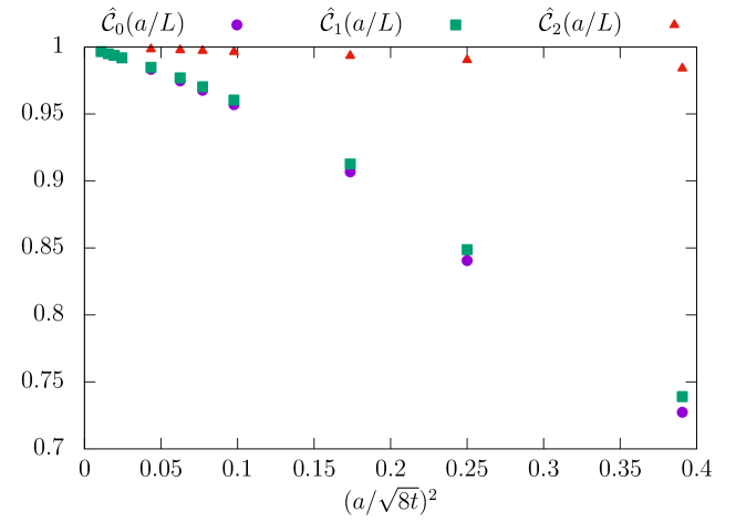
Figure 3: Cutoff effects in the usual step scaling function ($\hat{\mathcal{C}_{0}}(a/\sqrt{8t})$), compared to those in $\mathcal{J}_{1}$ (see $\hat{\mathcal{C}_{1}}(a/\sqrt{8t})$) and $\mathcal{J}_{2}$ (see $\hat{\mathcal{C}_{2}}(a/\sqrt{8t})$). See text for more details. Here we show the case of the Zeuthen flow/improved observable with plaquette gauge action (i.e. the same setup that will be used in our non-perturbative study).

Figure 3 shows the perturbative results. As the reader can see, the cutoff effects in $\hat{\mathcal{C}_{0}}(a/\sqrt{8t})$ are very similar to those in $\hat{\mathcal{C}_{1}}(a/\sqrt{8t})$. This can be understood in a simple way, since both these functions involve a change in the renormalization scale by a factor two. The main difference between both cases is that $\hat{\mathcal{C}_{1}}(a/\sqrt{8t})$ can be determined using lattice spacings that are a factor two smaller, since its determination does not require any change in the lattice size. The determination of $\hat{\mathcal{C}_{2}}(a/\sqrt{8t})$ does not involve any change in the renormalization scale, and it shows cutoff effects that are one order of magnitude smaller than either $\hat{\mathcal{C}_{0}}(a/\sqrt{8t})$ or $\hat{\mathcal{C}_{1}}(a/\sqrt{8t})$.

In the next section we will show that indeed these properties hold non-perturbatively, and that they are not a coincidence of leading order perturbation theory.

2.2.2 Non-perturbative study

In this section we will describe the non-perturbative results used in this study, first to support the claim that the numerical determination of $\hat{\mathcal{J}}_{2}$ has very small scaling violations, due to the fact that the renormalization scale is not changed (i.e. the determination of $\hat{\mathcal{J}}_{2}$ amounts to measuring finite volume effects in the coupling). Then, we want to show that the determination of $\mathcal{J}_{1}$ can be performed accurately even at values of $c$ that are too small to allow for a conservative estimate of the step scaling function.

All the analysis have been performed using two different analysis codes: one [16] based on the $\Gamma$-method [16, 17, 18, 19], and the other using a jackknife resampling technique. Both analysis techniques take into account the correlations between observables measured on the same ensemble. This is crucial, both for the determination of $J_{1}$ that involves the measurements of $\bar{g}^{2}$ on the same configuration at different values of the flow time, and also to correctly determine the uncertainty in the composition $J_{2}\circ J_{1}$.

Description of the data set

For our non-perturbative study we are going to use exactly the same dataset of [13]. This setup includes simulations of the pure gauge theory with the Wilson plaquette action on a lattice of size $L^{4}$ and lattice spacing $a$. We have several resolutions, $L/a=8,10,12,16,20,24,32,48$, at a large range of lattice spacings $a$ and with Schrödinger Functional (SF) boundary conditions. The setup is the same as the one used for the perturbative study in section 2.2.1.

We have measurements of the GF coupling at values of $c=0.2,0.3,0.4$ with two different discretizations: the usual Wilson flow/Clover observable and the Zeuthen flow/improved observable (more details can be found in [13]). Our target will be to determine the running non-perturbatively in the scheme defined by $c=0.2$ by computing the associated step scaling function $\sigma(u)$. Note that in reference [13] the value $c=0.3$ was used because the large scaling violations at $c=0.2$ did not allow for a determination of $\sigma(u)$.

We will revisit this attempt at a direct determination of $\sigma(u)$ here. Moreover, together with the data at $c=0.4$, we will be able to determine both $\mathcal{J}_{1},\mathcal{J}_{2}$, and compare their composition with the direct determination of $\sigma$.

Finally, the data with $c=0.3$ will be used in section 4 to compare the results of [13] (where the $\Lambda$ parameter is obtained by using a direct determination of the step scaling function with $c=0.3$) with our new strategy.

We will focus our investigations on the high energy regime, where $\bar{g}^{2}\sim 1-3$. Note that this region showed significant scaling violations, and in fact turns out to be the most delicate part of the analysis in the extraction of $\Lambda$ (see [13] for more details).

Scaling violations in $\mathcal{J}_{2}$

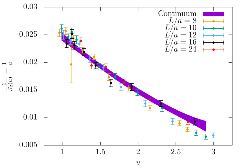
(a) Results for the combination of eq. (2.15) and continuum extrapolation from global fit.

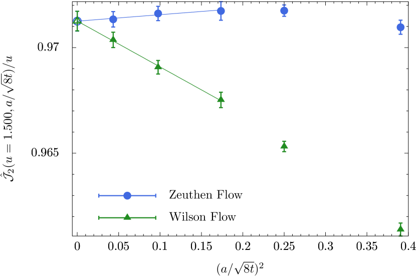
(b) Results for the $\hat{\mathcal{J}_{2}}(u,a/\sqrt{8t})/u$ ratio for $u=1.5$ for different discretizations. The continuum extrapolation is also included.

Figure 4: Results for the $\hat{\mathcal{J}_{2}}(u,a/\sqrt{8t})$ function and continuum extrapolation.

Let us start by investigating the scaling violations of $\mathcal{J}_{2}$. It is convenient to study the combination

$$\frac{1}{\hat{\mathcal{J}}_{2}(u,a/\sqrt{8t})}-\frac{1}{u}=f_{2}(u,a/\sqrt{8t})\,.$$ (2.15)

The continuum limit of the right hand side, $f_{2}(u,0)$, has an asymptotic expansion (in perturbation theory) as a polynomial in $u$, starting with a constant term. Note that our data set allows to determine $\hat{\mathcal{J}}_{2}(u,a/\sqrt{8t})$ for a factor three change in $a/\sqrt{8t}$.

The numerical raw data for $\hat{\mathcal{J}}_{2}(u,a/\sqrt{8t})$ is shown in figure 4(a). We also include in the plot the continuum extrapolation. At this point we defer the discussion on how this continuum curve is determined to section 4, and focus on the key element: the non-perturbative data for $\hat{\mathcal{J}}_{2}$ show very small scaling violations for all values of the coupling under study. The continuum curve is at most two standard deviations away from the coarser lattice data ($\sqrt{8t}/a\approx 1.6$), and the two finest lattices with $\sqrt{8t}/a\approx 3.2,4.8$ show no significant deviation from the continuum value.

One can look in more detail at the previous statement by interpolating the data with different $L/a$ to a common value of $u$, and then look at the continuum extrapolation of $\hat{\mathcal{J}}_{2}$. We choose the value $u=1.5$, where we have several points at each $L/a$, and therefore the necessary interpolations can be performed in the safest conditions available. Figure 4(b) shows that the Zeuthen flow data shows no significant scaling violations in the whole range of lattice spacing. The Wilson flow data show some scaling violations, but they are rather mild, with the finest lattice being almost compatible with the continuum value. Extrapolations of the data with both discretizations are in full agreement with each other.

Scaling violations in $\mathcal{J}_{1}$

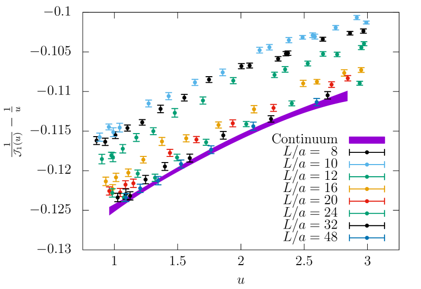
(a) Results for the combination of eq. (2.16) and continuum extrapolation from global fit.

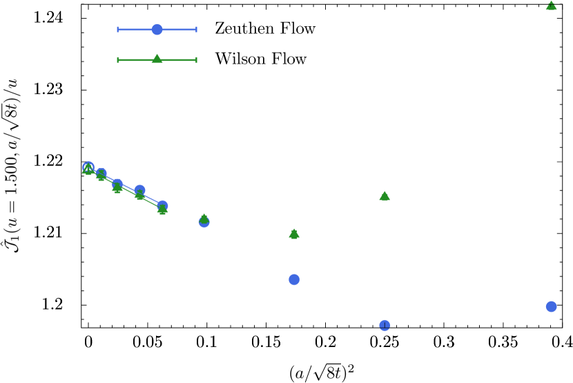
(b) Results for the $\hat{\mathcal{J}_{1}}(u,a/\sqrt{8t})/u$ ratio for $u=1.5$ for different discretizations. The continuum extrapolation is also included.

Figure 5: Results for the $\hat{\mathcal{J}_{1}}(u,a/\sqrt{8t})$ function and continuum extrapolation.

Once more, it is convenient to study the quantity

$$\frac{1}{\hat{\mathcal{J}}_{1}(u,a/\sqrt{8t})}-\frac{1}{u}=f_{1}(u,a/\sqrt{8t})\,.$$ (2.16)

The crucial difference with the previous case is that the determination of $\mathcal{J}_{1}$ involves a change in renormalization scale $\mu\to\mu/2$, so we expect significant scaling violations. On the other hand, its determination does not require to double the lattice sizes. In practice we have a range in lattice spacing that spans a factor 2 further.

Figure 5(a) shows a comparison of the raw data with the continuum curve (see section 4 for a discussion on its determination). In contrast with the case of $\hat{\mathcal{J}}_{2}$, we observe significant scaling violations, confirming our hypothesis that such violations are mainly a result of changes in the renormalization scale. Moreover, they show a complicated functional form: the three coarser lattices with $\sqrt{8t}/a=1.6,2.0,2.4$ do not show a monotonous pattern. The data is several standard deviations away from the continuum curve. Figure 5(b) shows again the continuum extrapolation of $\mathcal{J}_{1}(u)$ at the fixed value $u=1.5$. The plot confirms that scaling violations are significant, with the different discretizations based on the Wilson/Zeuthen flow showing differences of several standard deviations for $\sqrt{8t}/a<3.2$.

Still, one can obtain an accurate extrapolation of $\mathcal{J}_{1}$. In order to do so, the large range of lattice spacings available to us, from $L/a=8$ to $L/a=48$, is crucial. This is of course possible only because the determination of $\mathcal{J}_{1}$ does not require to double the lattice size. Figure 5(a) shows that the two finest lattices are in agreement with the continuum curve. Note however that these are very fine lattices with $\sqrt{8t}/a\approx 6.4,9.6$.

A detailed comparison with a direct determination of $\sigma_{0.2}(u)$

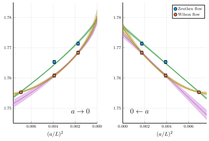
Figure 6: Continuum extrapolation of $\Sigma_{c=0.2}(u,a/\sqrt{8t})$ for $u=1.5$.
Right: extrapolations of the Zeuthen flow data with a functional form of the type $p_{0}+p_{1}(a/L)^{2}$. For the case of the Wilson flow one can extend the fitting range by including a quadratic term in the extrapolation $\mathcal{O}(a^{4})$. The extrapolated values show a reasonable agreement.
Left: the same data is extrapolated including logarithmic terms in the functional ansatze. For the case of the Zeuthen flow we use $p_{0}+p_{1}(a/L)^{2}\log(a/L)$, while for the case of the Wilson flow, we use functional forms $p_{0}+p_{1}(a/L)^{2}\log^{2}(a/L)$ and a three parameter ansatze $p_{0}+p_{1}(a/L)^{2}\log^{2}(a/L)+(a/L)^{4}$ that allows to extend the fitting range.
Summary: The extrapolated values vary significantly with the choice of logarithmic terms.

Finally, let us compare our new strategy with the direct determination of the step scaling function $\sigma_{c=0.2}$. Let’s start by stating what is known. The leading cutoff effects of the step scaling function $\Sigma$ can be described thanks to the Symanzik effective theory[22, 23, 24]. The asymptotic scaling violations have the form

$$\Sigma(u,a/\sqrt{8t})-\sigma(u)\sim a^{2}\log^{-\gamma}(a)+\dots\,.$$ (2.17)

Here $\gamma$ is related with an anomalous dimension. Its value depends both on the details of the gauge action simulated and the details of the observable $\Sigma$. Only recently [20] the leading relevant anomalous dimension for the special case of spectral quantities (in the pure gauge theory) has been computed. Except in this case, the relevant values of the leading anomalous dimensions are unknown.

The usual linear extrapolations in $\mathcal{O}(a^{2})$ are therefore only justified as long as the extrapolated values do not depend significantly on the (unknown) values of the anomalous dimensions $\gamma$.

Figure 6 shows the extrapolation of $\Sigma_{c=0.2}(u,a/\sqrt{8t})$ for $u=1.5$ as a representative example. The right panel shows linear extrapolations in $a^{2}$ for the Zeuthen flow data, and both linear and quadratic extrapolations for the Wilson flow data. The linear extrapolation of the Zeuthen flow data and the quadratic extrapolation of the Wilson flow data show an almost perfect agreement, with the linear extrapolation of the two finer lattice spacings of the Wilson flow data showing also a two-sigma agreement.

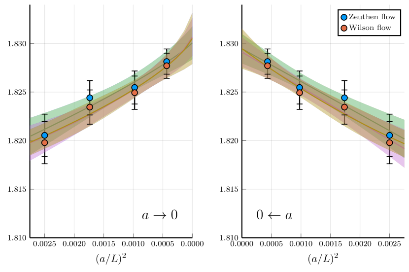
Figure 7: Continuum extrapolation of $\mathcal{J}_{1}(u,a/\sqrt{8t})$ for $u=1.5$. See text for discussion.
Right: extrapolations of the Zeuthen flow data with a functional form of the type $p_{0}+p_{1}(a/L)^{2}$. For the case of the Wilson flow one can extend the fitting range by including a quadratic term in the extrapolation $\mathcal{O}(a^{4})$. The extrapolated values show a reasonable agreement.
Left: the same data is extrapolated including logarithmic terms in the functional ansatze. For the case of the Zeuthen flow we use $p_{0}+p_{1}(a/L)^{2}\log(a/L)$, while for the case of the Wilson flow, we use functional forms $p_{0}+p_{1}(a/L)^{2}\log^{2}(a/L)$ and a three parameter ansatze $p_{0}+p_{1}(a/L)^{2}\log^{2}(a/L)+(a/L)^{4}$ that allows to extend the fitting range.
Summary: In contrast with the case of the direct extrapolation of $\Sigma$ (see figure 6), all explored choices of functional form show a very good agreement in the extrapolated values.

But this consistent picture is just hiding the assumptions that are behind such extrapolations. In particular, the left panel shows that using linear extrapolations in $a^{2}\log(a)$ (for the Zeuthen flow data) or linear extrapolations in $a^{2}\log^{2}(a)$ (for the Wilson flow data), one obtains an even better agreement. Unfortunately the perfectly consistent extrapolations without logarithmic terms do not agree with the perfectly consistent extrapolations that include such terms. The largest difference is between the Zeuthen flow extrapolation in $a^{2}\log(a)$ (with result 1.78341(88)), and the two-point linear extrapolation in $a^{2}$ of the Wilson flow data (with result 1.7744(10)), that differ by approximatley 7 combined sigmas. This just shows that the direct extrapolation of $\Sigma_{c=0.2}$, although statistically very precise, has an uncontrolled systematic uncertainty unless very large lattices are simulated.

Figure 7 shows the equivalent extrapolation for the case of $\mathcal{J}_{1}$. In this case one can see that the extrapolations with or without logarithmic terms agree nicely. The largest deviation is found in the extrapolation of the Zeuthen flow data with term $a^{2}\log(a)$ (with result 1.8309(19)), and the $a^{2}$ linear extrapolation of the Wilson flow data (with result 1.8291(15)). This discrepancy is less than one combined sigma. We conclude that the uncertainty in $\mathcal{J}_{1}(u)$ is in fact dominated by the statistical uncertainty, and not by our prejudice on the unknown values of the anomalous dimensions.

3 Statistical uncertainties

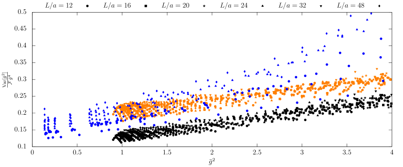
Figure 8: Results for the quantity of eq. (3.4) for three different datasets and six different lattice spacings. Orange symbols are for the “magnetic” definition of the GF coupling; black symbols are for the average of “magnetic” and “electric” definitions of the GF coupling; the blue symbols are from the dataset of ref. [25].

It has been argued that a simple way to improve the scaling properties of GF couplings consists in using large values of $c$ (see for example the discussion in [26]). Unfortunately, it is well known that this comes at the cost of increased statistical uncertainties. In this section we want to make this last statement more precise. We will present a simple model for the understanding of the scaling of the statistical uncertainties of the GF coupling and then we will show how the results of numerical simulations agree with this naive approach.

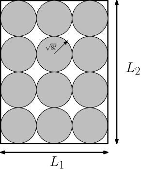
Figure 9: A simple model to explain the scaling of the variance of the GF coupling.

Let us first focus our discussion on schemes that fully preserve the translational invariance, like the case of periodic [4] or twisted [27] boundary conditions. The gradient flow smears the original gauge field $A_{\mu}(x)$ over a distance $d\sim\sqrt{8t}$. Due to the invariance under translations, each four dimensional ball of radius $\sqrt{8t}$ provides an estimate of the quantity $\langle E(x,t)\rangle$ (see figure 9). Under this assumption the volume average on a lattice $L_{0}\times L_{1}\times L_{2}\times L_{3}$ will make the variance of the observable $\langle E(x,t)\rangle$ proportional to

$$\mathcal{F}=\prod_{\mu=0}^{3}\frac{\sqrt{8t}}{L_{\mu}}\,.$$ (3.1)

Note that in the common situation of an $L^{4}$ lattice with the same length in all directions one has $\mathcal{F}=c^{4}$ (see equation (2.5)). This gives a quantitative explanation to the fact that the statistical uncertainties are large at large values of $c$.

In schemes where the invariance under translations is broken in the time direction, like Schrödinger Functional (SF) [5] or open-SF [15] boundary conditions on a box of sizes $L_{0}\times L_{1}\times L_{2}\times L_{3}$, a similar argument applies, except that in these cases the coupling is only measured at a single time-slice $x_{0}=L_{0}/2$. Therefore in this case we expect a factor

$$\mathcal{F}=\prod_{\mu=1}^{3}\frac{\sqrt{8t}}{L_{\mu}}\,,$$ (3.2)

e.g. on a symmetric lattice $\mathcal{F}=c^{3}$. When do we expect this model to break down? For the volume average argument to make sense, the region that is smeared by the flow must be much smaller than the size of the lattice, so we require

$$\frac{\sqrt{8t}}{L_{\mu}}\ll 1/2\,.$$ (3.3)

Note that for the case of an $L^{4}$ lattice this condition just means $c\ll 0.5$. The typical values used in the literature are $c=0.2-0.4$, so we can only expect the scaling of the variance to be approximate. In order to see how good this approximation is, it is useful to have a look at the quantity

$$\frac{{\rm Var}[\bar{g}^{2}]}{\mathcal{F}\bar{g}^{4}}\approx K(\bar{g}^{2})\,.$$ (3.4)

If our hypothesis is correct, we expect this combination to be independent on the lattice size and on the values of $\sqrt{8t}/L_{\mu}$. Figure 8 shows this quantity in three data sets.

First, in orange we plot the usual magnetic coupling definition that we have been using for our non-perturbative study (section 2.2.2). This data includes values of $c=0.200,0.225,0.250,\dots,0.400$ for lattices of sizes $L/a=12,16,20,24,32,48$ at several values of the bare coupling $\beta=6/g_{0}^{2}$. Note that, despite the fact that the lattice size changes by a factor of four, and that the values of $c$ change by a factor two, the combination in equation (3.4) shows a very mild variation in all the range of couplings $\bar{g}^{2}=1-4$. The plot shows some variation, but to a reasonably good approximation we can say that $Q(\bar{g}^{2})\approx 0.25$. An even better description of the data can be obtained by using a simple linear approximation.

Second, in black, we have another definition of the coupling in the same datasets (in particular the lattice sizes and values of $c$ are the same as in the previous case). The data corresponds to the coupling definition based on the space-time components of the Energy density (i.e. the average between the “magnetic” and the “electric” components). Despite the high correlation between the electric and magnetic energy densities, the average shows a significant smaller variance. In this the combination of equation (3.4) can also be reasonably well described by a linear function.

Finally, in blue, we have data with twisted boundary condition on an asymmetric lattice [25]. In this case the simulations are done on volumes $L^{2}\times(L/3)^{2}$ (see [28] for the theoretical motivation behind this particular geometry). We use data with $\sqrt{8t}/L=0.20,0.25,\dots,0.4$ and lattice sizes $L/a=12,24,48$. Note that in this particular case the condition equation (3.3) is flagrantly violated in the two short directions, since $3\sqrt{8t}/L=0.6-1.2$. This may explain why this dataset shows a much larger dispersion. For this case the combination in equation (3.4) shows a larger dependence on details like the particular choices of $L/a$ and $\sqrt{8t}$ and not only on $\bar{g}^{2}$. Still, the variation is not large taking into account the disparity of scales (varying by several factors) involved in the data (note that naively the variance changes by more than two orders of magnitude).

It is also worth mentioning that the variance at weak coupling is very similar for the three datasets, differing by at most a factor three. Together with the observation that being a flow observable, the quantity in equation (3.4) has a well defined continuum limit, we can conclude that the function in equation (3.4) is universal. Details like the choice of boundary conditions or the choices of discretizations induce relatively small scaling violations, especially at the weakest couplings.

4 The high energy regime of Yang-Mills revisited

As a further test on our proposal, we will re-examine the high energy regime of Yang-Mills. Let us first recall the relevant points of the work [13].

• The determination of the $\Lambda_{\overline{\rm MS}}$ parameter in units of $\sqrt{8t_{0}}$ is divided in two fundamental pieces. First, a high energy part where contact with perturbation theory is made. This results in a determination of $\Lambda_{\overline{\rm MS}}/\mu_{\rm ref}$, with $\mu_{\rm ref}$ being defined by $\bar{g}_{c=0.3}^{2}(\mu_{\rm ref})=0.8\pi$. Second, a low energy part where the dimensionless ratio $\mu_{\rm ref}\times\sqrt{8t_{0}}$ is determined.

• Most of the error in the dimensionless ratio

  $$\Lambda_{\overline{\rm MS}}\times\sqrt{8t_{0}}=\frac{\Lambda_{\overline{\rm MS}}}{\mu_{\rm ref}}\times(\mu_{\rm ref}\sqrt{8t_{0}})\,,$$ (4.1)

  comes from the first piece (i.e. the high energy part). The total uncertainty in $\Lambda_{\overline{\rm MS}}\times\sqrt{8t_{0}}$ is 1.57%, while the uncertainty in $\Lambda_{\overline{\rm MS}}/\mu_{\rm ref}$ is already 1.37%.

• The result for $\Lambda_{\overline{\rm MS}}\times\sqrt{8t_{0}}=0.6227(98)$ shows a significant discrepancy with other determinations: in particular the very precise determination of FlowQCD [29] $\Lambda_{\overline{\rm MS}}\times\sqrt{8t_{0}}=0.5934(38)$ lies about 3 sigma away from the value of [13].

Given that the pure gauge determination of $\Lambda_{\overline{\rm MS}}$ has to face the very same challenges as the determination of the strong coupling $\alpha_{s}(M_{\rm Z})$ in QCD, we think that revising the crucial part of the work [13] with the new method proposed in this work is fully justified. We recall that our dataset is exactly the same as the one used in [13] (see section 2.2.2).

4.1 The continuum limit of $\mathcal{J}_{1}$ and $\mathcal{J}_{2}$

In order to obtain the functions $\mathcal{J}_{1}$ and $\mathcal{J}_{2}$ in the continuum, the best strategy consists in combining the continuum extrapolation with a parametrization of the function in the continuum. In particular we are going to use the parametrization

$$\frac{1}{\hat{\mathcal{J}}_{i}(u,a/\sqrt{8t})}-\frac{1}{u}=\sum_{n=0}^{n_{\rm c}}c_{n}^{(i)}u^{n}+\left(\frac{a}{\sqrt{8t}}\right)^{2}\,\sum_{n=0}^{n_{\rho}}\rho_{n}^{(i)}u^{n}\,.$$ (4.2)

Note that the coefficients $c_{n}^{(i)}$ parametrize the continuum function $\mathcal{J}_{i}(u)$, while the coefficients $\rho_{n}^{(i)}$ parametrize the $\mathcal{O}(a^{2})$ cutoff effects in the function $\hat{\mathcal{J}}_{i}$. There are several assumptions hidden in this parametrization. First we assume that the continuum function $1/\hat{\mathcal{J}}_{i}(u,0)-1/u$ can be well described by a polynomial. This is certainly the case in perturbation theory to all orders, and we expect that the non-perturbative functions can be well described by a polynomial ansatz.

A more delicate assumption is that in our functional form of equation (4.2) all scaling violations are quadratic (i.e. $a^{2}/(8t)$). First, due to the breaking of translational invariance in the Schrödinger Functional, we expect cutoff effects linear in the lattice spacing. They are expected to be small, due to the localization of the GF coupling at the timeslice $x_{0}=T/2$. Moreover the extrapolations in section 2.2.2 have completely ignored these effects, and our data in fact seem to scale like $\mathcal{O}(a^{2})$ after dropping the coarser lattices. But due to the high precision of our data, these $\mathcal{O}(a)$ effects cannot be completely ignored, especially if we take into account the fact that our strategy uses data at large values of $\sqrt{8t}/T=0.4$, where these effects are expected to be larger than in [13], where $\sqrt{8t}/T=0.3$ was used. For this reason we include a generous estimate of these linear effects in the error. The details are explained in Appendix A.

Our data set has also higher order cutoff effects, of the form $a^{n}$ for $n>2$, and logarithmic corrections as well [20]. The effect of these terms in our extrapolations will be estimated by changing the cuts used to fit the coefficients $c_{n}^{(i)},\rho_{n}^{(i)}$.

4.1.1 The case $\mathcal{J}_{1}$

In the exploratory study in section 2.2.2 the Zeuthen flow/improved observable discretization already displayed better scaling properties, but still we had to discard all lattices with $L/a<12$. Since the Wilson flow/Clover combination would require even more stringent cuts, we will only use the improved setup to quote final results.

		$u$
	Parameters	1.125	1.250	1.500	1.750	2.000
$L/a\geq 12$	$n_{\rm c}=3,\,n_{\rho}=2$	1.30681(46)	1.47575(54)	1.82918(82)	2.2044(12)	2.6029(17)
	$n_{\rm c}=4,\,n_{\rho}=2$	1.30681(46)	1.47575(54)	1.82918(82)	2.2044(13)	2.6029(18)
$L/a\geq 16$	$n_{\rm c}=3,\,n_{\rho}=2$	1.30658(49)	1.47549(54)	1.82882(85)	2.2038(13)	2.6020(19)
	$n_{\rm c}=4,\,n_{\rho}=2$	1.30658(49)	1.47547(55)	1.82880(85)	2.2039(14)	2.6021(20)
$L/a\geq 20$	$\mathbf{n_{\rm c}=3,\,n_{\rho}=2}$	1.30640(59)	1.47535(61)	1.82878(96)	2.2039(16)	2.6021(23)
	$n_{\rm c}=3,\,n_{\rho}=3$	1.30637(59)	1.47550(67)	1.8291(12)	2.2040(16)	2.6014(25)
	$n_{\rm c}=3,\,n_{\rho}=4$	1.30633(59)	1.47549(66)	1.8291(12)	2.2040(16)	2.6014(25)
	$n_{\rm c}=4,\,n_{\rho}=2$	1.30639(59)	1.47539(62)	1.82881(96)	2.2038(16)	2.6019(23)

Table 1: Values of the continuum function $\mathcal{J}_{1}(u)$ for different fit parametrizations and cuts (see equation (4.2)). In bold we show our preferred fit. See text for more details.

This is confirmed by looking at table 1, where the values in the continuum of $\mathcal{J}_{1}(u,0)$ are shown at a few representative values of $u$. As the reader can see, the effect of varying the number of fit parameters ($n_{\rm c}$ and $n_{\rho}$ in equation (4.2)) is negligible. On the other hand, the cut in $L/a$ has a small effect on the extrapolations. If lattices with $L/a=12$ are included, the continuum value of $\mathcal{J}_{1}$ seems to be systematically higher, but still compatible within errors. Also the statistical errors are smaller for these analysis. A conservative approach consists in just taking a fit with $L/a\geq 20$ (i.e. $a/\sqrt{8t}<1/4$), so that the continuum value has a larger uncertainty. Note that since the computation of $\mathcal{J}_{1}$ does not require to double the lattice sizes, even with this stringent cut our dataset still offers more than a factor two in lattice spacing. Among these fits there is very little difference between different parametrizations. Moreover the fit quality is very similar in all cases. All in all we just choose one of these fits ($n_{\rm c}=3$, $n_{\rho}=2$, bold in table 1) as our final result.

4.1.2 The case $\mathcal{J}_{2}$

		$u$
	Parameters	1.125	1.250	1.500	1.750	2.250
All $L/a$	$n_{\rm c}=3,n_{\rho}=2$	1.09602(61)	1.21647(67)	1.45772(97)	1.6999(14)	2.1879(23)
	$n_{\rm c}=4,n_{\rho}=2$	1.09607(62)	1.21640(67)	1.45764(96)	1.7000(14)	2.1879(23)
$L/a\geq 10$	$n_{\rm c}=3,n_{\rho}=2$	1.09640(68)	1.21677(70)	1.45778(96)	1.6996(14)	2.1871(24)
	$n_{\rm c}=4,n_{\rho}=2$	1.09647(69)	1.21672(70)	1.45770(96)	1.6997(14)	2.1871(24)
$L/a\geq 12$	$\mathbf{n_{\rm c}=3,n_{\rho}=2}$	1.09629(82)	1.21652(81)	1.4572(10)	1.6986(16)	2.1859(28)
	$n_{\rm c}=3,n_{\rho}=3$	1.09621(89)	1.21658(82)	1.4574(13)	1.6988(17)	2.1852(35)
	$n_{\rm c}=3,n_{\rho}=4$	1.09629(89)	1.21672(83)	1.4575(13)	1.6985(17)	2.1843(36)
	$n_{\rm c}=4,n_{\rho}=2$	1.09650(85)	1.21641(81)	1.4569(11)	1.6986(16)	2.1858(28)

Table 2: Values of the continuum function $\mathcal{J}_{2}(u)$ for different fit parametrizations and cuts (see equation (4.2)). In bold we show our preferred fit. See text for more details.

The computation of $\mathcal{J}_{2}$ requires to double the lattice sizes, and then our datasets offers only half the lever arm in lattice spacing for the continuum extrapolations. Our hypothesis is that the scaling violations are small for $\mathcal{J}_{2}$ because its determination does not involve a change in renormalization scale. Our preliminary investigation of section 2.2.2 has also confirmed this hypothesis. Table 2 shows that this is indeed the case. Even including the coarser lattices with $L/a=8$ (corresponding to $a/\sqrt{8t}=1/1.6$), the results are in agreement within errors. It is clear that the choice of parametrization has very little effect. We just settle for one particular fit with $L/a\geq 12$ (represented in bold in table 2) that we will use for any further analysis.

4.2 The quantity $\sqrt{8t_{0}}\times\Lambda_{\overline{\rm MS}}$

4.2.1 The scale $\mu_{\rm ref}$

As we have already mentioned, the original work [13] determined the dimensionless combination $\sqrt{8t_{0}}\times\Lambda_{\overline{\rm MS}}$ as the product of two factors. First the low energy factor

$$\sqrt{8t_{0}}\mu_{\rm ref}=7.808(46)\qquad[0.59\%]\,,$$ (4.3)

that has a very small uncertainty. The other factor $\Lambda_{\overline{\rm MS}}/\mu_{\rm ref}$ was much more delicate to determine. It is precisely this last quantity that we want to determine once more with our new strategy. A first step consists in dealing with the factor $\mu_{\rm ref}$. This was defined in the scheme with $c=0.3$ by the condition

$$\bar{g}^{2}_{c=0.3}(\mu_{\rm ref})=\frac{4\pi}{5}\approx 2.5132\ldots\,.$$ (4.4)

Since our new strategy provides the step scaling function $\sigma(u)$ for $c=0.2$, we must first determine the value of our coupling $\bar{g}_{c=0.2}(\mu_{\rm ref})$. The procedure is completely analogous to the determination of $\mathcal{J}_{1}$. We first define

$$\hat{\mathcal{J}}_{3}(u,a/\sqrt{8t})=\bar{g}^{2}_{c=0.3}(2\mu/3)\Big{|}_{\bar{g}^{2}_{c=0.2}(\mu)=u}\,.$$ (4.5)

We choose to fit our data to the model

$$\frac{1}{\hat{\mathcal{J}}_{3}(u,a/\sqrt{8t})}-\frac{1}{u}=\sum_{n=0}^{n_{\rm c}}c_{n}^{(3)}u^{n}+\left(\frac{a}{\sqrt{8t}}\right)^{2}\,\sum_{n=0}^{n_{\rho}}\rho_{n}^{(i)}u^{u}\,.$$ (4.6)

The same considerations discussed in section 4.1.1 apply to the determination, in the continuum, of the relation between $\bar{g}^{2}_{c=0.2}(\mu)$ and $\bar{g}^{2}_{c=0.3}(\mu)$. In this case, however, we expect the scaling violations to be smaller, since the change in renormalization scale is not a factor two, but only a factor 3/2.

We performed several fits, changing the number of fit parameters $n_{\rm c}$ and $n_{\rho}$, and using different cuts for our data, and the overall analysis results in a consistent value for $\bar{g}_{c=0.2}(\mu_{\rm ref})$ as long as data with $L/a\geq 16$ is used.

We choose to quote the result with $n_{\rm c}=3$ and $n_{\rho}=2$ and $L/a\geq 20$

$$\bar{g}^{2}_{c=0.2}(\mu_{\rm ref})=2.17621(84)\,.$$ (4.7)

Despite the high precision, the result should be actually considered conservative, as this particular fit has one of the largest uncertainties of all the combinations that we tried (see figure 10).

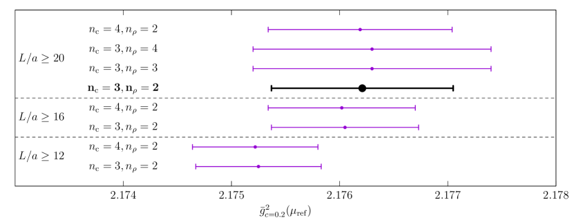
Figure 10: Determination of $\bar{g}^{2}_{c=0.2}(\mu_{\rm ref})$ using different parametrizations and cuts. In black and bold face the result of equation (4.7)).

4.2.2 The extraction of $\Lambda_{\overline{\rm MS}}$

The $\Lambda_{s}$-parameter in the scheme defined by the coupling $\bar{g}_{s}^{2}$ is given by the expression

$$\frac{\Lambda_{s}}{\mu}=\left[b_{0}\bar{g}_{s}^{2}(\mu)\right]^{-\frac{b_{1}}{2b_{0}^{2}}}\,e^{-\frac{1}{2b_{0}\bar{g}_{s}^{2}(\mu)}}\,\exp\{-I_{s}(\bar{g_{s}}(\mu))\},\quad I_{s}(g)=\int_{0}^{g}{\rm d}x\,\left[\frac{1}{\beta_{s}(x)}+\frac{1}{b_{0}x^{3}}-\frac{b_{1}}{b_{0}^{2}x}\right]\,.$$ (4.8)

Note that this expression is exact, and valid beyond perturbation theory, as long as the non-perturbative $\beta$-function, defined by

$$\mu\frac{{\rm d}}{{\rm d}\mu}\bar{g}_{s}(\mu)=\beta_{s}(\bar{g})\,.$$ (4.9)

is known. If two renormalized couplings are related to one-loop by the expression

$$\bar{g}^{2}_{s^{\prime}}(\mu)=\bar{g}^{2}_{s}(\mu)+c_{ss^{\prime}}\bar{g}^{4}_{s}(\mu)+\dots$$ (4.10)

the corresponding $\Lambda$-parameters are related by

$$\frac{\Lambda_{s^{\prime}}}{\Lambda_{s}}=\exp\left(\frac{-c_{ss^{\prime}}}{2b_{0}}\right)\,.$$ (4.11)

This last formula allows for a non-perturbative definition of $\Lambda_{\overline{\rm MS}}$, even if the $\overline{\rm MS}$ scheme is intrinsically perturbative.

All in all, the determination of $\Lambda_{\overline{\rm MS}}$ requires the determination of the integral in equation (4.8) in a scheme that is non-perturbatively defined. The lower limit of the integral is zero, which requires to determine the $\beta$-function up to infinite energy. In practice this can only be achieved by a limit process. One first defines

$$K_{s}(\bar{g}_{s}(\mu),g_{\rm PT})=\int_{g_{\rm PT}}^{\bar{g}_{s}(\mu)}{\rm d}x\,\left[\frac{1}{\beta_{s}(x)}+\frac{1}{b_{0}x^{3}}-\frac{b_{1}}{b_{0}^{2}x}\right]+\int_{0}^{g_{\rm PT}}{\rm d}x\,\left[\frac{1}{\beta_{s}^{(l)}(x)}+\frac{1}{b_{0}x^{3}}-\frac{b_{1}}{b_{0}^{2}x}\right]\,,$$ (4.12)

very similar to the previous function $I_{s}(\bar{g}_{s}(\mu))$. The only difference is that the integral in equation (4.8) for values of the coupling smaller than $g_{\rm PT}$ is determined by substituting the $\beta_{s}$-function by its $l$-loop perturbative approximation $\beta_{s}^{(l)}(x)$

$$\beta_{s}(x)\raisebox{-0.43057pt}{ $\stackrel{{\scriptstyle\small{x\to 0}}}{{\sim}}$}\beta_{s}^{(l)}(x)=-x^{3}\sum_{n=0}^{l}b_{n}x^{2n}+\mathcal{O}(x^{2(l+1)})\,.$$ (4.13)

The first two coefficients $b_{0}=11/(4\pi)^{2}$ and $b_{1}=102/(4\pi)^{4}$ are scheme-independent, while the values $b_{n}$ for $n>1$ depend on the chosen scheme. It is now clear that

$$K_{s}(\bar{g}_{s}(\mu),g_{\rm PT})\raisebox{-0.43057pt}{ $\stackrel{{\scriptstyle\small{g_{\rm PT}\to 0}}}{{\sim}}$}I_{s}(\bar{g}_{s}(\mu))+\mathcal{O}(g_{\rm PT}^{2(l-1)})\,,$$ (4.14)

In practice for most finite volume schemes, the $\beta_{s}$-function is known up to three loops, and therefore the corrections are $\mathcal{O}(g_{\rm PT}^{4})$. The value of the coupling $g_{\rm PT}$ delimits the energy region (from $\mu_{\rm PT}$ to $\infty$) where perturbation theory is used via the relation

$$\bar{g}_{s}^{2}(\mu_{\rm PT})=g_{\rm PT}^{2}\,.$$ (4.15)

Ideally one would like to estimate the $\Lambda$-parameter by taking the following limit

$$\frac{\Lambda_{s}}{\mu}=\lim_{g_{\rm PT}\to 0}\left\{\left[b_{0}\bar{g}_{s}^{2}(\mu)\right]^{-\frac{b_{1}}{2b_{0}^{2}}}\,e^{-\frac{1}{2b_{0}\bar{g}_{s}^{2}(\mu)}}\,\exp\{-K_{s}(\bar{g_{s}}(\mu),g_{\rm PT})\}\right\}\,.$$ (4.16)

Since the value of the coupling $\bar{g}^{2}_{s}(\mu)$ runs logarithmically with $\mu$, it is technically a challenge to probe a large range of energy scales so that the corrections $\mathcal{O}(g^{2(l-1)}_{\rm PT})$ vary substantially and the limit can be taken accurately.

Of course finite-size scaling was designed to explore such large ranges of energy scales. Starting from the scale $\mu_{\rm ref}$ (see section 4.2.1), and with the knowledge of the step scaling function $\sigma=\mathcal{J}_{2}\circ\mathcal{J}_{1}$ (see section 4.1), one can define the sequence of couplings

$$u_{0}=\bar{g}^{2}(\mu_{\rm ref})\,,\qquad u_{n}=\sigma^{-1}(u_{n-1})=\mathcal{J}_{1}^{-1}\left(\mathcal{J}_{2}^{-1}(u_{n-1})\right)=\bar{g}^{2}(2^{n}\mu_{\rm ref})\,.$$ (4.17)

The energy scales reached by this procedure increase geometrically. Contact with perturbation theory can be made at each step by choosing $g^{2}_{\rm PT}=u_{n}$ in equation (4.14), and one can indeed check that the corrections $\mathcal{O}(u_{n}^{2})$ are small and decrease as they should. For a long time, the challenge was mainly to maintain a high precision, but the most recent works [31, 13] have shown that when one reaches a high precision, the corrections can be significant in some schemes even at very high energy scales.

	GF		SF		$\overline{\rm MS}$ $(s=1)$		$\overline{\rm MS}$ $(s=2)$
$n$	$\bar{g}^{2}(\mu_{n})$	$\sqrt{8t_{0}}\,\Lambda_{\overline{\rm MS}}$	$\bar{g}^{2}_{\rm SF}(0.3\mu_{n+1})$	$\sqrt{8t_{0}}\,\Lambda_{\overline{\rm MS}}$	$\bar{g}^{2}_{\overline{\rm MS}}(0.3\mu_{n+1})$	$\sqrt{8t_{0}}\,\Lambda_{\overline{\rm MS}}$	$\bar{g}^{2}_{\overline{\rm MS}}(0.3\mu_{n+2})$	$\sqrt{8t_{0}}\,\Lambda_{\overline{\rm MS}}$
0	2.17621(84)	0.6714(33)	2.008(10)	0.6179(99)	2.554(16)	0.5615(85)	2.037(11)	0.6112(97)
1	1.7734(22)	0.6596(49)	1.6553(24)	0.6252(46)	2.0087(36)	0.5850(42)	1.6732(25)	0.6205(45)
2	1.4989(28)	0.6527(67)	1.4091(25)	0.6270(62)	1.6566(34)	0.5972(58)	1.4211(25)	0.6237(62)
3	1.2992(27)	0.6479(83)	1.2280(24)	0.6267(77)	1.4112(32)	0.6037(74)	1.2366(25)	0.6242(77)
4	1.1471(25)	0.6442(95)	1.0890(23)	0.6252(90)	1.2302(29)	0.6070(87)	1.0955(23)	0.6233(90)
5	1.0273(24)	0.641(11)	0.9789(22)	0.623(11)	1.0911(28)	0.608(10)	0.9839(22)	0.621(11)
$\infty$	Linear	0.631(15)		0.621(16)		0.618(14)		0.621(16)
$\infty$	Constant	-		0.6260(74)		-		0.6234(73)

Table 3: Sequence of couplings in different schemes and at different scales ($\mu_{n}=2^{n}\mu_{\rm ref}$) and the corresponding values of $\sqrt{8t_{0}}\,\Lambda_{\overline{\rm MS}}$ (see text for more details). The values of $\bar{g}(\mu_{n})$ are obtained via a recursive application of the step scaling function in the GF scheme (equation (4.17)). The conversion from the GF scheme to the SF scheme is performed non-perturbatively and detailed in appendix B. The conversion to the $\overline{\rm MS}$ scheme is done by using the perturbative relation with the SF scheme (equation (4.19)). The last two rows show possible extrapolations of $\sqrt{8t_{0}}\,\Lambda_{\overline{\rm MS}}$ using the last four values ($n=2,3,4,5$). We show both an extrapolation linear in the $\bar{g}^{4}$ and a extrapolation to a constant for the cases that this behavior is compatible with the data.

For this reason reaching high energies alone is not enough. The limit in equation (4.16) has to be taken seriously and the systematics well estimated. Fortunately our dataset allows us to study the matching with perturbation theory at energy scales

$$\mu_{n}=2^{n}\mu_{\rm ref}\,,\qquad\left(n=0,\dots,5\right)\,.$$ (4.18)

Moreover we will explore several options to match with perturbation theory:

GF:

This is just the direct application of equation (4.8) using $g^{2}_{\rm PT}=u_{n}$ to determine $I_{\rm GF}(\bar{g}(\mu_{n}))$ (cf. equation (4.14)). Schematically:

$$u_{n}=\bar{g}^{2}(\mu_{n})\xrightarrow[(\text{eq.}~{}(\ref{eq:lamdef}))]{\beta^{(3)}_{\rm GF}}\frac{\Lambda_{\rm GF}}{\mu_{\rm ref}}\xrightarrow{\frac{\Lambda_{\overline{\rm MS}}}{\Lambda_{\rm GF}}}\frac{\Lambda_{\overline{\rm MS}}}{\mu_{\rm ref}}\,.$$

In this case the matching with perturbation theory is performed in the GF scheme at a scale $\mu_{\rm PT}=\mu_{n}=2^{n}\mu_{\rm ref}$.

SF:

Reference [13] showed that schemes based on the GF show a very poor perturbative convergence. The same reference suggested to match non-perturbatively to the traditional SF coupling [32] with background field. The details of this matching are explained in appendix B. Schematically:

$$u_{n}=\bar{g}^{2}(\mu_{n})\xrightarrow[(\text{ap}.~{}\ref{sec:matching-with-sf})]{\text{GF}\to\text{SF}}\bar{g}^{2}_{\rm SF}(0.3\,\mu_{n+1})\xrightarrow[(\text{eq.}~{}(\ref{eq:lamdef}))]{\beta^{(3)}_{\rm SF}}\frac{\Lambda_{\rm SF}}{\mu_{\rm ref}}\xrightarrow{\frac{\Lambda_{\overline{\rm MS}}}{\Lambda_{\rm SF}}}\frac{\Lambda_{\overline{\rm MS}}}{\mu_{\rm ref}}\,.$$

In this case matching with perturbation theory is performed in the SF scheme at a scale $\mu_{\rm PT}=0.3\times\mu_{n+1}=0.3\times 2^{n+1}\mu_{\rm ref}$.

$\overline{\mbox{MS}}$:

One can convert the values of the SF coupling to the $\overline{\rm MS}$ scheme using the perturbative relation [33]

$$\bar{g}^{2}_{\overline{\rm MS}}(s\mu)=\bar{g}^{2}_{\rm SF}(\mu)+\frac{c_{1}(s)}{4\pi}\bar{g}^{4}_{\rm SF}(\mu)+\frac{c_{2}(s)}{(4\pi)^{2}}\bar{g}^{6}_{\rm SF}(\mu)+\dots\,.$$ (4.19)

where

$$c_{1}(s) = -8\pi b_{0}\log s+1.255621(2)\,,$$ (4.20a)

$$c_{2}(s) = c_{1}^{2}(s)-32\pi^{2}b_{1}\log(s)+1.197(10)\,.$$ (4.20b)

Once the value of the coupling in the $\overline{\rm MS}$ scheme is known, one can use the known 5-loop $\beta$-function [34] to determine directly $\Lambda_{\overline{\rm MS}}$. Even if the running is known much more accurately in the $\overline{\rm MS}$ scheme, this procedure carries the same parametric uncertainty $\mathcal{O}(\bar{g}^{4}_{\overline{\rm MS}})$ as the others, since the limiting factor is represented by the known orders in the perturbative relation between couplings, equation (4.19) (see [31]). Schematically we have

$$u_{n}=\bar{g}^{2}(\mu_{n})\xrightarrow[(\text{ap}.~{}\ref{sec:matching-with-sf})]{\text{GF}\to\text{SF}}\bar{g}^{2}_{\rm SF}(0.3\,\mu_{n+1})\xrightarrow[(\text{eq.~{}(\ref{eq:sftoms})})]{\text{SF}\to\overline{\rm MS}}\bar{g}^{2}_{\overline{\rm MS}}(s\,0.3\,\mu_{n+1})\xrightarrow[(\text{eq.}~{}(\ref{eq:lamdef}))]{\beta^{(5)}_{\overline{\rm MS}}}\frac{\Lambda_{\overline{\rm MS}}}{\mu_{\rm ref}}\,.$$

In this case the scale of matching with perturbation theory is performed in the SF scheme at a scale $\mu_{\rm PT}=s\,0.3\times 2^{n+1}\mu_{\rm ref}$, but the RG evolution is done in the $\overline{\rm MS}$ scheme. The value of $s$ is in principle arbitrary, but if taken too large the perturbative coefficients of equation (4.20) become large, and one expects a bad asymptotic convergence of the perturbative series. We will explore two choices: first the simple $s=1$, and then the value $s=2$, that is very close to the value of fastest apparent convergence .

The values of $\Lambda_{\overline{\rm MS}}/\mu_{\rm ref}$ can be multiplied by the factor $\sqrt{8t_{0}}\,\mu_{\rm ref}$ (cf. equation (4.3)) to produce the results for $\sqrt{8t_{0}}\,\Lambda_{\overline{\rm MS}}$ reported in table 3 according to the different procedures. In the next section we will comment on the results.

4.2.3 Results and discussion

We refer the reader once more to table 3. The values for $\sqrt{8t_{0}}\,\Lambda_{\overline{\rm MS}}$ differ for the different treatments of perturbation theory. There are two important points worth mentioning:

1. Even at scales where $\bar{g}^{2}\approx 1$ (corresponding to $\alpha\approx 0.08$), different treatments of perturbation theory produce values of $\sqrt{8t_{0}}\,\Lambda_{\overline{\rm MS}}$ that vary as much as 3%.

2. There are two particular treatments of perturbation theory (labeled SF and $\overline{\rm MS}(s=2)$), where the value of $\sqrt{8t_{0}}\,\Lambda_{\overline{\rm MS}}$ is constant within errors when extracted over a range of energy scales that vary by a factor 32.

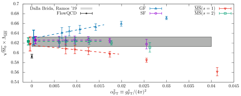
Figure 11: The dimensionless product $\sqrt{8t_{0}}\times\Lambda_{\overline{\rm MS}}$ as a function of $g_{\rm PT}$ (see equation (4.16)). The empty symbols represent the data of table 3 for $n=0,\dots,5$, while the filled symbols are extrapolations $g_{\rm PT}\to 0$ (shifted for better visibility) of the different approaches to the perturbative matching (see text for more details). The gray band is the result of reference [13], while the data point labeled FlowQCD is the result of reference [29].

These results are also plotted in figure 11. Qualitatively we see that the variations between different treatments of perturbation theory roughly scale as expected (i.e. decrease proportionally to $\alpha^{2}$).

A more quantitative picture is obtained by looking at the two last rows of table 3. They show possible extrapolations of the quantity $\sqrt{8t_{0}}\,\Lambda_{\overline{\rm MS}}$ (see equation (4.16)): the deviation from the final result of reference [13] $\sqrt{8t_{0}}\,\Lambda_{\overline{\rm MS}}=0.6227(98)$ of any of the possible extrapolations is below the statistical uncertainties (about $1.5\%$). This is half of the differences present at scales where $\bar{g}^{2}\approx 1$.

All extrapolations $g_{\rm PT}\to 0$ agree well (last two rows of table 3). In particular even the extrapolations that assume that the higher order terms proportional to $g^{4}_{\rm PT}$ are negligible show quite a small uncertainty. Still, the error band covers the central values of all other extrapolations. Note however that the size of the uncertainties depends strongly on how much data one decides to include. A very conservative approach (such as the one used in reference [13]) would consist in just quoting as final result the value at the most perturbative point. This is justified since the data labeled SF and $\overline{\rm MS}\,(s=2)$ shows basically no dependence on the value of $g_{\rm PT}$.

Note however that the methodology in these two works is very different. In particular they deal with the systematic associated with the continuum extrapolations in a very different way. Reference [13] uses the GF coupling with $c=0.3$ in order to perform the non-perturbative running. On the other hand we use the step scaling function with $c=0.2$, determined as the composition of the functions $\mathcal{J}_{1}$ and $\mathcal{J}_{2}$ as described in section 2.2 order to do the non-perturbative running. Even with the highly conservative approach that we used in section 4.1 to perform the continuum extrapolations of $\hat{\mathcal{J}_{1}}$ and $\hat{\mathcal{J}_{2}}$, we find a final uncertainty on $\sqrt{8t_{0}}\,\Lambda_{\overline{\rm MS}}$ of the same size of the one obtained in reference [13]. Moreover, the fact that the central values are in perfect agreement in the two calculations provides very strong evidence that the systematic effects associated with the continuum extrapolations are completely under control, and well below our statistical uncertainties.

Finally, the extrapolations that assume a linear dependence in $\alpha_{\rm PT}^{2}$ show larger uncertainties. Still, it is very important to see that the $g_{\rm PT}\to 0$ extrapolation substantially improves the agreement between all treatments of the perturbative matching.

It is also worth mentioning that the propagation of the linear $\mathcal{O}(a)$ effects (see appendix A) represent about a 15% of the final error squared in $\sqrt{8t_{0}}\,\Lambda_{\overline{\rm MS}}$. This is about a 50% larger than in the extraction of reference [13] and can be understood noting that making use of values of the coupling at $c=0.4$, we increase the boundary effects.

All in all our approach shows a remarkable agreement between very different treatments of the matching with perturbation theory, and thanks to our new proposal, we are able to also show a very good agreement with previous works that have rather different systematics associated with the continuum extrapolation.

4.2.4 Scale uncertainties

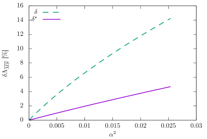
Figure 12: Scale uncertainties for $\Lambda$ associated to different renormalization scales for the coupling $\bar{g}^{2}_{\overline{\rm MS}}(s\mu)$. The solid curve (labeled $\delta^{\star}$) shows the perturbative uncertainty estimated by varying the scale around the scale of fastest apparent convergence. The dashed curve (labeled $\delta$) shows the perturbative uncertainty estimated by varying the scale around the physical scale. See text for more details.

The approach labeled $\overline{\rm MS}$ in section 4.2.2 is very close to many phenomenological extractions of the strong coupling. The value of $\bar{g}^{2}_{\overline{\rm MS}}$ is extracted from a measurement, in this case from the value of the SF coupling obtained in a simulation, thanks to its perturbative expansion

$$\bar{g}^{2}_{\overline{\rm MS}}(s\mu)=\bar{g}^{2}_{\rm SF}(\mu)+\frac{c_{1}(s)}{4\pi}\bar{g}^{4}_{\rm SF}(\mu)+\frac{c_{2}(s)}{(4\pi)^{2}}\bar{g}^{6}_{\rm SF}(\mu)+\dots\,.$$

Different renormalization scales $s\mu$ can be used for each value of the physical scale $\mu$. The differences between different renormalization scales are an estimate of the truncation errors (i.e. an estimate of the $\mathcal{O}(g_{\rm PT}^{2(l-1)})$ effects in equation (4.14)). In particular, in phenomenology, it is very common to vary the renormalization scale a factor two above/below some chosen value.

Figure 12 shows such estimate of the uncertainties propagated to the $\Lambda$-parameter. $\delta^{\star}$ is obtained by varying the renormalization scale of a factor two above/below the scale of fastest apparent convergence (i.e. the average difference between the values of $\Lambda$ obtained after using $s=1$ and $s=2$ and then $s=2$ and $s=4$).

From figure 12 it is clear that that scales uncertainties are rather large in the pure gauge theory. Even at $\alpha\approx 0.1$, corresponding to the highest scales reached in our study, they are around 2%. One might question the results of our works, that claim a significantly smaller uncertainty. The key to claim smaller errors than the scale uncertainties lies in the limit definition of $\Lambda$, equation (4.16). Once the limit $g_{\rm PT}\to 0$ is properly taken, and its systematic estimated, one does not need to talk about the uncertainties at non-zero $g_{\rm PT}$. Of course taking such a limit is hard: data at different values of $g_{\rm PT}$ is required. Due to the logarithmic running of the coupling with the physical energy scale, the apparently innocent limit of equation (4.16) requires to solve a hard multi-scale problem. Even with our datasets, that spans a factor 32 in energy scales (a change in the coupling $g_{\rm PT}^{2}$ by more than a factor two), we have seen that some assumptions on the scaling as $g_{\rm PT}\to 0$ are needed in order to reach the 1.4% precision on $\Lambda$.

We consider our approach to treat perturbative uncertainties very conservative. Still, future works in the pure gauge theory might want to explore even larger energy scales.

5 Conclusions

In this work we have examined the main sources of uncertainties present in finite-size scaling studies using the Gradient Flow: the continuum extrapolation and the statistical uncertainties. We have argued that scaling violations are a result of exploring changes in the flow time. This observation has been supported both by a perturbative study and by non-perturbative numerical results.

The determination of the step scaling function $\sigma(u)$, the crucial observable in step scaling studies, involves both a change in the flow time and a change in the size of the system. We propose to divide the determination of $\sigma(u)$ in two pieces: first, a change in the renormalization scale at a constant size of the system (the function $\mathcal{J}_{1}$), followed by a change of the size of the system at constant renormalization scale (the function $\mathcal{J}_{2}$). The advantage is that, according to our hypothesis, only the first step shows significant cutoff effects. By breaking up the determination in two pieces, the scaling violations can be studied much more accurately. Modest datasets allow to explore a change of the renormalization scale at constant physical volume with lattice spacings varying by factors 4-6. In section 2.2 we have seen that this strategy usually comes at the cost of larger statistical uncertainties, especially in schemes like the Schrödinger Functional that break translation invariance and have to deal with $\mathcal{O}(a)$ systematic effects. Thus, the proposal trades the large systematic associated with the continuum extrapolations present in many GF studies with a statistical uncertainty. Since the latter are much easier to control, we think that the proposed strategy shows a clear advantage. In section 3 we have shown that statistical uncertainties can be well understood and predicted with a simple model.

We think that this strategy can shed some light in many problems that are currently being studied where systematic effects of the continuum extrapolation are relevant (see for example the recent discussion in [7]). A detailed study of the scaling violations of $\mathcal{J}_{1}$, that according to our hypothesis are very similar to those of the step scaling function $\sigma$, should become a standard way to assess the quality of the continuum determination of the step scaling function. This is specially relevant for studies of the conformal window, since much less is known about the logarithmic corrections to scaling in this model, and as we have shown in section 2.2.2 they can have a large effect in the extrapolations.

We have also re-examined the determination of the $\Lambda$-parameter in the pure gauge theory. The most crucial step is the high energy region and the matching with the asymptotic perturbative regime. We have used the step scaling function with $c=0.2$, determined using our new proposal. The matching with perturbation theory is performed in different schemes and using different procedures. Our datasets allows to match with perturbation theory at energy scales $\mu_{\rm PT}$ where $\alpha(\mu_{\rm PT})\lesssim 0.1$. Even at this large energy scales the perturbative truncation effects are large, corresponding to about a $2\%$ uncertainty in $\Lambda$. The size of this uncertainty is also confirmed by a scale variation analysis. All in all, perturbative errors are large in the pure gauge theory, making the determination of $\Lambda$ rather challenging in this aspect, in particular when compared with the corresponding determination in QCD. Fortunately, our dataset explores a large range of energy scales, and gives us the possibility to explore the limit $\alpha(\mu_{\rm PT})\to 0$ (corresponding to $\mu_{\rm PT}\to\infty$). Once this limit is properly taken, the perturbative uncertainties at $\alpha(\mu_{\rm PT})$ estimated using scale variation or any other procedure are irrelevant. Of course taking such a limit is very challenging. The corrections, $\mathcal{O}(\alpha^{2}(\mu_{\rm PT}))$, decrease very slowly due to the logarithmic running of the coupling at high energies.

Taking the limit $\alpha_{\rm PT}\to 0$ is very challenging in a large volume setup due to the finite range of scales that any lattice simulation can probe. This might explain the difference with some precise results in large volume [29], although a more detailed study is necessary.

Depending on the assumptions made in the extrapolation $\alpha(\mu_{\rm PT})\to 0$, the uncertainty in $\Lambda$ varies in the range $1-2\%$. All in all, our results show a perfect agreement with the final result of [13] ($\sqrt{8t_{0}}\times\Lambda_{\overline{\rm MS}}=0.6227(98)$), obtained with $c=0.3$, that quotes an uncertainty $\approx 1.4\%$. We stress once more that the method that we used in this work provides a careful control on the continuum extrapolations, leading to a final uncertainty on $\sqrt{8t_{0}}\times\Lambda_{\overline{\rm MS}}$ of the same size of [13] even when using a very conservative approach. Due to the different treatments of perturbation theory and the use of different schemes, it seems clear that, despite some discrepancies with other works (see discussion in [13]), the systematic effects in [13] are well under control.

Appendix A Boundary $\mathcal{O}(a)$ effects

The procedure to estimate the $\mathcal{O}(a)$ cutoff effects is completely analogous as in [13]. In fact we use the same datasets. We determine numerically the dependence of the GF coupling at different values of $c=0.2,0.3,0.4$ with the boundary parameter $c_{t}$. This is done using simulations at different values of the improvement parameter $c_{t}$ close to its 2-loop value

$$c_{t}^{\star}(g_{0})=1-0.089g_{0}^{2}-0.0294g_{0}^{4}+\mathcal{O}(g_{0}^{6})\,,\qquad(g_{0}^{2}=6/\beta)\,,$$ (A.1)

for lattice sizes $L/a=8,10,12$. This allows to obtain

$$\frac{\partial\bar{g}^{2}_{c}}{\partial c_{t}}\Big{|}_{c_{t}=c_{t}^{\star}}=\frac{a}{L}\left[a_{0}(c)\bar{g}_{c}^{2}+a_{1}(c)\bar{g}_{c}^{4}\right]\,.$$ (A.2)

Table 4 shows the result of the parameters $a_{0}(c),a_{1}(c)$.

	$c=0.2$	$c=0.3$	$c=0.4$
$a_{0}(c)$	0.04(3)	-0.14(5)	-0.88(7)
$a_{1}(c)$	-0.11(2)	-0.26(3)	-0.43(3)

Table 4: Values of the fit coefficients $a_{0}(c)$ and $a_{1}(c)$ that parameterize the sensitivity of $\bar{g}^{2}_{c}$ to the boundary improvement coefficient $c_{t}$.

Now we need an estimate of how much the true, non-perturbative, value of $c_{t}$ differs from its 2-loop value. There is no information available, but the extrapolations at constant $u$ of section 2.2.2 completely ignored this linear effects and the data showed no significant deviation from a $\mathcal{O}(a^{2})$ scaling. This suggests that these effects are smaller than our statistical uncertainties. With this insight, a conservative approach consists in using the full 2-loop contribution as an estimate of the difference between the 2-loop value and the correct non-perturbative one.

In summary we add to all our data, in quadratures, the error

$$\delta\bar{g}_{c}^{2}=\frac{a}{L}\left[a_{0}(c)\bar{g}_{c}^{2}+a_{1}(c)\bar{g}_{c}^{4}\right]\times 0.0294g_{0}^{2}\,.$$ (A.3)

in order to account for a possible mis-tuning of the boundary $\mathcal{O}(a)$-improvement parameter $c_{t}$.

Appendix B Matching with the SF scheme

Since the strategy is the same as the one used in [13], we refer the interested reader to this reference for more details.

Here it is enough to say that we performed a set of SF simulations with background field and lattice sizes $L/a=6,8,10,12,16$ and at the same values of the bare coupling $g_{0}^{2}=6/\beta$ as the available measurements of the GF coupling in twice the lattice size $L/a=12,16,20,24,32$. We collect between $9\times 10^{5}$ and $2\times 10^{6}$ measurements of the SF coupling $\bar{g}^{2}_{\rm SF}$. We further remove all cutoff effects up to 2 loops from $\bar{g}^{2}_{\rm SF}$ (i.e. the leading cutoff effects are $\mathcal{O}(g_{0}^{6})$). The non-perturbative data is fitted to a functional form of the type

$$\frac{1}{\bar{g}^{2}_{\rm SF}(\mu)}-\frac{1}{\bar{g}^{2}_{c=0.3}(\mu/(2c))}=f(u)+\left(\frac{a}{L}\right)^{2}\tilde{\rho}(u),\qquad(u=\bar{g}^{2}_{c=0.3}(\mu/(2c)))\,,$$ (B.1)

where both $f(u)$ and $\tilde{\rho}(u)$ are simple polynomials in $u$. For the GF coupling we use the measurements at $c=0.3$. The matching with other values of $c$ is performed thanks to the knowledge of the function $\mathcal{J}_{3}$ of equation (4.5).

To quote all our results we use the same fit used in reference [13], where the coarser lattice is dropped from the fit and the functions $f(u),\tilde{\rho}(u)$ are degree two polynomials.

References

- [1] R. Narayanan and H. Neuberger, “Infinite N phase transitions in continuum Wilson loop operators,” JHEP 0603 (2006) 064, arXiv:hep-th/0601210 [hep-th].
- [2] M. Lüscher, “Properties and uses of the Wilson flow in lattice QCD,” JHEP 1008 (2010) 071, arXiv:1006.4518 [hep-lat].
- [3] M. Lüscher, P. Weisz, and U. Wolff, “A Numerical method to compute the running coupling in asymptotically free theories,” Nucl.Phys. B359 (1991) 221–243.
- [4] Z. Fodor, K. Holland, J. Kuti, D. Nogradi, and C. H. Wong, “The Yang-Mills gradient flow in finite volume,” JHEP 1211 (2012) 007, arXiv:1208.1051 [hep-lat].
- [5] P. Fritzsch and A. Ramos, “The gradient flow coupling in the Schrödinger Functional,” JHEP 1310 (2013) 008, arXiv:1301.4388 [hep-lat].
- [6] A. Ramos, “The gradient flow running coupling with twisted boundary conditions,” JHEP 1411 (2014) 101, arXiv:1409.1445 [hep-lat].
- [7] O. Witzel, “Review on Composite Higgs Models,” PoS LATTICE2018 (2019) 006, arXiv:1901.08216 [hep-lat].
- [8] A. Ramos, “The Yang-Mills gradient flow and renormalization,” PoS LATTICE2014 (2015) 017, arXiv:1506.00118 [hep-lat].
- [9] C. J. D. Lin, K. Ogawa, H. Ohki, A. Ramos, and E. Shintani, “SU(3) gauge theory with 12 flavours in a twisted box,” arXiv:1410.8824 [hep-lat].
- [10] Z. Fodor, K. Holland, J. Kuti, S. Mondal, D. Nogradi, et al., “The lattice gradient flow at tree-level and its improvement,” JHEP 1409 (2014) 018, arXiv:1406.0827 [hep-lat].
- [11] A. Ramos and S. Sint, “Symanzik improvement of the gradient flow in lattice gauge theories,” Eur. Phys. J. C76 no. 1, (2016) 15, arXiv:1508.05552 [hep-lat].
- [12] ALPHA Collaboration, M. Dalla Brida, P. Fritzsch, T. Korzec, A. Ramos, S. Sint, and R. Sommer, “Slow running of the Gradient Flow coupling from 200 MeV to 4 GeV in QCD,” Phys. Rev. D95 no. 1, (2017) 014507, arXiv:1607.06423 [hep-lat].
- [13] M. Dalla Brida and A. Ramos, “The gradient flow coupling at high-energy and the scale of SU(3) Yang-Mills theory,” arXiv:1905.05147 [hep-lat].
- [14] M. Lüscher and P. Weisz, “Perturbative analysis of the gradient flow in non-abelian gauge theories,” JHEP 1102 (2011) 051, arXiv:1101.0963 [hep-th].
- [15] M. Lüscher, “Step scaling and the Yang-Mills gradient flow,” JHEP 1406 (2014) 105, arXiv:1404.5930 [hep-lat].
- [16] A. Ramos, “Automatic differentiation for error analysis of Monte Carlo data,” Comput. Phys. Commun. 238 (2019) 19–35, arXiv:1809.01289 [hep-lat].
- [17] ALPHA Collaboration, U. Wolff, “Monte Carlo errors with less errors,” Comput.Phys.Commun. 156 (2004) 143–153, arXiv:hep-lat/0306017 [hep-lat].
- [18] N. Madras and A. D. Sokal, “The pivot algorithm: A highly efficient monte carlo method for the self-avoiding walk,” Journal of Statistical Physics 50 no. 1, (Jan, 1988) 109–186. https://doi.org/10.1007/BF01022990.
- [19] F. Virotta, Critical slowing down and error analysis of lattice QCD simulations. PhD thesis, Humboldt-Universität zu Berlin, Mathematisch-Naturwissenschaftliche Fakultät I, 2012.
- [20] N. Husung, P. Marquard, and R. Sommer, “Asymptotic behavior of cutoff effects in Yang-Mills theory and in Wilson’s lattice QCD,” arXiv:1912.08498 [hep-lat].
- [21] J. Balog, F. Niedermayer, and P. Weisz, “The Puzzle of apparent linear lattice artifacts in the 2d non-linear sigma-model and Symanzik’s solution,” Nucl. Phys. B824 (2010) 563–615, arXiv:0905.1730 [hep-lat].
- [22] K. Symanzik, “Small distance behavior in field theory and power counting,” Commun. Math. Phys. 18 (1970) 227–246.
- [23] K. Symanzik, “Continuum Limit and Improved Action in Lattice Theories. 1. Principles and phi**4 Theory,” Nucl. Phys. B226 (1983) 187.
- [24] K. Symanzik, “Schrodinger Representation and Casimir Effect in Renormalizable Quantum Field Theory,” Nucl.Phys. B190 (1981) 1.
- [25] E. I. Bribian, M. Garcia Perez, and A. Ramos, “The twisted gradient flow running coupling in SU(3): a non-perturbative determination,” in 37th International Symposium on Lattice Field Theory (Lattice 2019) Wuhan, Hubei, China, June 16-22, 2019. 2020. arXiv:2001.03735 [hep-lat].
- [26] C. J. D. Lin, K. Ogawa, and A. Ramos, “The Yang-Mills gradient flow and SU(3) gauge theory with 12 massless fundamental fermions in a colour-twisted box,” JHEP 12 (2015) 103, arXiv:1510.05755 [hep-lat].
- [27] A. Ramos, “The gradient flow in a twisted box,” PoS Lattice2013 (2014) 053, arXiv:1308.4558 [hep-lat].
- [28] E. I. Bribian and M. Garcia Perez, “The twisted gradient flow coupling at one loop,” arXiv:1903.08029 [hep-lat].
- [29] M. Kitazawa, T. Iritani, M. Asakawa, T. Hatsuda, and H. Suzuki, “Equation of State for SU(3) Gauge Theory via the Energy-Momentum Tensor under Gradient Flow,” Phys. Rev. D94 no. 11, (2016) 114512, arXiv:1610.07810 [hep-lat].
- [30] Dalla Brida, Mattia and Lüscher, Martin, “SMD-based numerical stochastic perturbation theory,” Eur. Phys. J. C77 no. 5, (2017) 308, arXiv:1703.04396 [hep-lat].
- [31] ALPHA Collaboration, M. Dalla Brida, P. Fritzsch, T. Korzec, A. Ramos, S. Sint, and R. Sommer, “A non-perturbative exploration of the high energy regime in QCD,” Eur. Phys. J. C78 no. 5, (2018) 372, arXiv:1803.10230 [hep-lat].
- [32] M. Lüscher, R. Narayanan, P. Weisz, and U. Wolff, “The Schrödinger Functional: a renormalizable probe for non-abelian gauge theories,” Nucl.Phys. B384 (1992) 168–228, arXiv:hep-lat/9207009 [hep-lat].
- [33] Alpha Collaboration, A. Bode, U. Wolff, and P. Weisz, “Two loop computation of the Schrodinger functional in pure SU(3) lattice gauge theory,” Nucl. Phys. B540 (1999) 491–499, arXiv:hep-lat/9809175 [hep-lat].
- [34] P. A. Baikov, K. G. Chetyrkin, and J. H. Kḧn, “Five-Loop Running of the QCD coupling constant,” Phys. Rev. Lett. 118 no. 8, (2017) 082002, arXiv:1606.08659 [hep-ph].