On Fast Retrial for Two-Step Random Access in MTC

Abstract

In machine-type communication (MTC), a group of devices or sensors may need to send their data packets with certain access delay limits for delay-sensitive applications or real-time Internet-of-Things (IoT) applications. In this case, 2-step random access approaches would be preferable to 4-step random access approaches that are employed for most MTC standards in cellular systems. While 2-step approaches are efficient in terms of access delay, their access delay is still dependent on re-transmission strategies. Thus, for a low access delay, fast retrial that allows immediate re-transmissions can be employed as a re-transmission strategy. In this paper, we study 2-step random access approaches with fast retrial as a buffered multichannel ALOHA with fast retrial, and derive an analytical way to obtain the quality-of-service (QoS) exponent for the distribution of queue length so that key parameters can be decided to meet QoS requirements in terms of access delay. Simulation results confirm that the derived analytical approach can provide a good approximation of QoS exponent.

I Introduction

There has been a surge of interest in the Internet-of-Things (IoT) [1] [2] [3] in various aspects including IoT connectivity [4] [5] [6]. While there exist a large number of devices to be connected, there are some devices that require low access delay for mission critical applications. To support a large number of devices, machine-type communication (MTC) has been studied in cellular systems (e.g., 5th generation (5G) systems) [7]. For low access delay applications, ultra-reliable low latency communication (URLLC) is also extensively investigated [8] [9].

In MTC, random access approaches are employed to support a number of devices with sporadic traffic due to low signaling overhead. In particular, handshaking processes based on random access are considered for MTC in standards [10] [11]. In general, a handshaking process consists of 4 steps and it is often called 4-step approach. In the first step, a device with data to send is to randomly choose a preamble from a pool of pre-determined preambles, which is shared by all the devices in a cell, and transmit it so that a base station (BS) can allocate a dedicated uplink channel to the device.

There are also other approaches. For example, 2-step random access approaches are extensively studied [12], which are also often called compressive random access or one-shot [13] [14] [15] [16] or grant-free approaches [17] [18] [19] [20]. There are several differences between 4-step and 2-step approaches. In 4-step approaches, two different uplink channels are used, namely physical random access channel (PRACH) and physical uplink shared channel (PUSCH). Preambles are transmitted through PRACH, while data packets are transmitted through PUSCH. On the other hand, in 2-step approaches, since both preamble and data packets are transmitted together, one physical channel can be used. In addition, in 2-step approaches, the length of data blocks is likely fixed [16]. Thus, 2-step approaches would be suitable for the case that devices have short messages and their lengths are more or less the same. Otherwise (i.e., the variation of message lengths is significant between devices), 4-step approaches would be preferable.

While the main advantage of 2-step approaches over 4-step approaches is a low access or transmission delay, which makes it more suitable for URLLC, the access delay of 2-step approaches is strongly dependent on re-transmission strategies due to collisions that are inevitable because 2-step approaches are contention-based access schemes. In particular, if a device has a data packet that has to be delivered with a high probability (or a low probability of packet dropping for highly reliable transmission requirement), it must be re-transmitted until it is successfully transmitted without collision. Thus, a proper re-transmission scheme has to be considered to meet requirements in terms of access delay. While there are a number of re-transmission strategies, in order to shorten transmission or access delay in MTC, fast retrial [21] [22] would be promising, in which another randomly selected preamble is to be immediately re-transmitted in the next slot.

In [23] [24] [25], performance analysis of 4-step random access approaches with various backoff schemes for re-transmissions is studied in terms of access delay. However, the delay analysis of 2-step random access approaches, which will be simply referred to as 2-step approaches, with fast retrial has not been well studied except [26]. In [26], buffered multichannel ALOHA with fast retrial is analyzed using the notion of effective bandwidth and effective capacity [27] [28], which allows us to see the delay performance in terms of quality-of-service (QoS) exponent or the tail probability of queue length without analyzing state transition probabilities in a multi-dimensional space. As will be discussed in the paper, since 2-step approaches with fast retrial can be seen as buffered multichannel ALOHA with fast retrial, the results in [26] can be utilized to decide key parameters in 2-step approaches with fast retrial. However, due to some approximations used in [26], there exists some gap between derived (analytic) QoS exponents and simulated ones. Thus, in this paper, in order to obtain more accurate results, the number of assumptions or approximations required for analysis is reduced. Consequently, a good approximation of the tail probability of queue length is obtained through an analytical way, which allows us to design 2-step approaches with fast retrial to meet low delay requirements.

The rest of the paper is organized as follows. In Section II, we present the system model for 2-step approaches and introduce fast retrial. The stability and steady-state analysis are considered in Section III without any particular arrival models. In Section IV, based on the notion of effective bandwidth and effective capacity, the QoS exponent is discussed for independent Poisson arrivals. Simulation results are presented in Section V and the paper is concluded in Section VI with a few remarks.

Notation

Matrices and vectors are denoted by upper- and lower-case boldface letters, respectively. The superscript ${\rm T}$ denotes the transpose. The support of a vector is denoted by ${\rm supp}({\bf x})$ (which is the number of the non-zero elements of ${\bf x}$). ${\mathbb{E}}[\cdot]$ and ${\rm Var}(\cdot)$ denote the statistical expectation and variance, respectively. ${\mathbb{Z}}=\{0,1,\ldots\}$ stands for the set of non-negative integers.

II System Model

Suppose that a system consists of a BS and $N$ devices, where $N\geq 1$, for MTC. It is assumed that all devices are synchronized (using beacon signals transmitted by the BS). To perform random access in MTC, devices share a pool of $L$ preambles. The length of preambles is denoted by $M$, which is proportional to the system bandwidth. If a device has messages to send to the BS, it can transmit a randomly selected preamble. Since the number of preambles is finite, multiple devices can choose the same preamble, which results in preamble collision.

In this paper, we focus on 2-step approaches for devices that need low access delay in delay-sensitive applications. In Fig. 1, an illustration of 2-step approaches is shown. The first and third steps in 4-step random access are to transmit a randomly selected preamble and a data packet, respectively, while these two steps are combined into the first step in 2-step random access. In the second step, the BS is to send a feedback signal so that devices can see whether or not collisions happen.

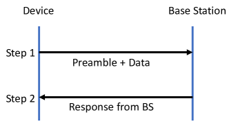
Figure 1: An illustration of 2-step random access approaches in MTC.

The first step in 2-step random access consists of two phases: the preamble and data transmission phases. A randomly selected preamble is to be transmitted in the first phase and then data packet transmission follows in the second phase as shown in Fig 2. In the second phase, i.e., the data transmission phases, $L$ mini-slots can be considered so that an active device that transmits preamble $l$ can transmit its data packet in the $l$th mini-slot [16]. Alternatively, as in [17], $L$ spreading sequences can be used for data packet transmissions by multiple active devices, where each spreading sequence is uniquely associated with a preamble. In any case, preamble collision leads to packet collision. For example, suppose there are $L$ mini-slots for the data transmission phase. If multiple devices choose preamble $l$, they will also transmit data packets in the $l$th mini-slot, which results in packet collision. Thus, in this paper, preamble collision is simply referred to as collision (as it leads to packet collision). If a device experiences collision (which is known by the feedback from the BS in the second step), it can drop message. Alternatively, it can try to re-transmit according to re-transmission strategies.

Figure 2: Two phases (i.e., preamble transmission and data transmission phases) for the first step in 2-step random access.

For re-transmissions in 2-step approaches, in this paper, fast retrial [21] is used to lower access delay [22]. With fast retrial in 2-step approaches, a device experiencing collision immediately re-transmit with another randomly selected preamble. Note that as there are multiple preambles, the resulting random access becomes multichannel ALOHA as in [21] [22]. Throughout the paper, it is assumed that the two steps can be carried out within a time slot and $t$ is used for the index of time slots, where $t\in\{0,1,\ldots\}$. In Fig. 3, we illustrate fast retrial with $L=4$ preambles. At slot $t$, suppose that devices 1 and 3 transmit preamble 1, which results in preamble collision. At the next time slot, i.e., slot $t+1$, the two devices re-transmit randomly selected preambles (preamble 2 for device 1 and preamble 4 for device 3), while a new active device, i.e., device 2, transmits preamble 1. In this case, all the devices can successfully transmit preambles. This shows that immediate re-transmissions by fast retrial may not lead to successive preamble collision (unlike single-channel ALOHA), and shorten the access delay (due to no back-off time).

Figure 3: An illustration of fast retrial with 3 (type-1) devices and 4 preambles.

As mentioned earlier, the resulting 2-step approach can be seen as multichannel ALOHA with fast retrial. Furthermore, for re-transmissions, each device has to have a buffer, which results in a buffered (slotted) multichannel ALOHA system.

III Stability and Steady-State Analysis

In this section, we study the stability of fast retrial in 2-step approaches and steady-state analysis. Throughout the paper, we assume that $L\geq 2$ (otherwise, fast retrial cannot be used).

III-A Stability

When any re-transmission strategy (e.g., fast retrial) is employed, each device needs to have a buffer to keep their data packets until they can be successfully transmitted. Denote by $q_{n}(t)$ the length or state of device $n$’s queue at time slot $t$. Let $a_{n}(t)$ be the number of arrivals at slot $t$. For simplicity, it is assumed that an arrival is equal to a data block that is to send with a preamble in the first step. For example, if $a_{n}(t)=2$, device $n$ needs at least 2 time slots to transmit two data blocks that are arrived at time $t$, because a device can send one data block at a time (within a time slot). Consequently, $q_{n}(t)\in\{0,1,\ldots\}$ can be written as

$$q_{n}(t+1)=(q_{n}(t)+a_{n}(t)-s_{n}(t))^{+},$$ (1)

where $(x)^{+}=\max\{0,x\}$ and $s_{n}(t)\in\{0,1\}$ is the number of data blocks that can be possibly transmitted without collision. That is,

$$s_{n}(t)=\left\{\begin{array}[]{ll}1,&\mbox{if no collision happens}\cr 0,&\mbox{o.w.}\cr\end{array}\right.$$ (2)

In general, it is expected that the length of queue, $q_{n}(t)$ is finite if the system is stable. Furthermore, for a low access delay, $q_{n}(t)$ has to be short, since the access delay is proportional to the queue length. Thus, it is important to analyze the state of queue, $q_{n}(t)$. As shown in (1), $q_{n}(t)$ can be seen as a Markov chain [29]. Unfortunately, the analysis of $q_{n}(t)$ is not straightforward as $s_{n}(t)$ depends on the other devices’ queue states, which means that the state of each queue is not independent and the analysis of a $N$-dimensional Markov chain, ${\bf q}(t)=[q_{1}(t)\ \ldots\ q_{N}(t)]^{\rm T}\in{\mathbb{Z}}^{N}$ is required to take into account the interaction between $N$ devices’ queues. In this paper, as will be explained later, however, we do not consider a conventional approach based on state transition probabilities (e.g., [23] [25]), but a simple approach that can allow to effectively see the distribution of queue length individually.

Although certain steady-state analysis has been carried out for fast retrial in [21] [22], the stability was not addressed. In [30] [31], based on Foster-Lyapunov criteria [32] [33], the stability of fast retrial has been studied. In particular, in [31], the following result is obtained.

Theorem 1

Suppose that $a_{n}(t)$ is independent and identically distributed (iid) with a finite mean as follows:

$$\lambda_{n}={\mathbb{E}}[a_{n}(t)]<\infty,$$ (3)

where $\lambda_{n}$ is the mean arrival rate of device $n$. If

$$\frac{1}{N}\sum_{n=1}^{N}\lambda_{n}<\left(1-\frac{1}{L}\right)^{N-1},$$ (4)

then ${\bf q}(t)$ is positive recurrent.

While the proof of Theorem 1 can be found in [31], it is necessary to highlight that the condition in (4) is a sufficient condition for stability. It can also be seen that the right-hand side (RHS) term in (4) is the probability of no collision (or successful transmission) when all $N$ devices transmit, which can be the worst case in terms of the average departure rate as all devices compete for $L$ preambles.

There are a number of observations based on (4). First of all, an asymptotic case can be considered with (4). Let $\eta=\frac{N}{L}$. With a fixed ratio $\eta$, as $N$ approaches $\infty$, we have

$$\lim_{N\to\infty}\left(1-\frac{1}{L}\right)^{N-1}=e^{-\eta}.$$ (5)

Thus, an asymptotic version of (4) becomes

$$\bar{\lambda}<e^{-\eta},$$ (6)

where $\bar{\lambda}=\lim_{N\to\infty}\frac{\sum_{n=1}^{N}\lambda_{n}}{N}$. It can also be shown that the queues may not be stable if $N\to\infty$ with non-zero $\lambda_{n}$ and a finite $L$. That is, for a fixed $L$, (4) becomes

$$\frac{\sum_{n=1}^{N}\lambda_{n}}{N}<e^{-\kappa_{L}(N-1)},$$ (7)

where $\kappa_{L}=\ln\frac{L}{L-1}$. Thus, as $N\to\infty$, when $\bar{\lambda}>0$, we see that the RHS term approaches 0 with a fixed $L$. This implies that when the number of devices can be unbounded as in [21], random backoff algorithms need to be used for the case that a device fails to transmit after a certain number of re-transmissions with fast retrial. Otherwise, the average arrival rate per device should decrease exponentially with $N$, i.e., the decrease of $\bar{\lambda}$ has to be faster than $1/N$. This shows that a large number of devices is not desirable for 2-step approaches with fast retrial to ensure low access delay unless $L$ is also large.

III-B Steady-State Analysis

Once the condition in (4) holds, a stationary distribution of ${\bf q}(t)$ exists, because ${\bf q}(t)$ is positive recurrent [29]. Thus, in this subsection, a steady-state analysis is carried out under the assumption that a stationary distribution of ${\bf q}(t)$ exists.

Let $K$ be the number of devices that send preambles at a slot in steady-state. Here, the index of time slots, $t$, is omitted for convenience. With a finite $N$, let $\lambda=\frac{\sum_{n=1}^{N}\lambda_{n}}{N}$. For a system in steady-state, the average total arrival rate is $\lambda N$, while the average total departure rate, which is the average number of the transmitted preambles without collision, is given by

$$G={\mathbb{E}}\left[K\left(1-\frac{1}{L}\right)^{K-1}\right].$$ (8)

In steady-state, they should be the same, i.e.,

$$\lambda N=G={\mathbb{E}}\left[K\left(1-\frac{1}{L}\right)^{K-1}\right].$$ (9)

For simplicity, let

$$\lambda_{n}=\lambda,\ n=1,\ldots,N.$$ (10)

Furthermore, it is assumed that the number of devices is larger than or equal to the number of preambles, i.e., $N\geq L$. The symmetric condition in (10) leads to the same probability of transmission (or access probability) for all devices, denoted by $\alpha$. Due to the interaction between queues, the events that devices transmit become dependent. However, for tractable analysis, we can consider an approximation that the events are independent, which leads to the following distribution of $K$:

$$\Pr(K=k)=\binom{N}{k}\alpha^{k}(1-\alpha)^{N-k},$$ (11)

i.e., $K$ follows a binomial distribution. Substituting (11) into (9), we have

$$\lambda=S(\alpha)\buildrel\triangle\over{=}\alpha\left(1-\frac{\alpha}{L}\right)^{N-1},$$ (12)

which can be used to find $\alpha$ from $\lambda$.

Lemma 1

For a given $\lambda<\lambda_{\rm max}$, where

$$\lambda_{\rm max}=\left(1-\frac{1}{L}\right)^{N-1},$$ (13)

there is a unique $\alpha$ that satisfies (12). Note that $\lambda<\lambda_{\rm max}$ implies (4).

Proof:

In (12), it can be readily shown that $S(\alpha)$ is a unimodal function (i.e., a $\cap$-shape) and has the maximum when $\alpha=\frac{L}{N}$. Thus, with $L\leq N$, we have

$$\bar{S} =\max_{0\leq\alpha\leq 1}S(\alpha)$$ (14)

$$=S\left(\frac{L}{N}\right)=\frac{L}{N}\left(1-\frac{1}{N}\right)^{N-1}\approx\frac{L}{N}e^{-1}.$$ (15)

As a result, if $\lambda\leq\bar{S}$, there can be two solutions that satisfy (12) (because $S(\alpha)$ has a $\cap$-shape). It can also be shown that

$$\bar{S}\geq S(1)=\lambda_{\rm max}.$$ (16)

One of the two solutions that satisfy $\lambda_{\rm max}=S(\alpha)$ is obviously $\alpha=1$ and the other is less than or equal to $\frac{L}{N}$, which is denoted by $\alpha_{\rm max}$, as shown in Fig. 4. In addition, for a $\lambda<\lambda_{\rm max}$, one of two solutions is less $\alpha_{\rm max}$ and the other has to be greater than $1$. Since $\alpha$ is a probability, it has to be less than or equal to 1, i.e., $\alpha\leq 1$, which implies that there is a unique solution $\alpha$ that satisfies (12) for $\lambda<\bar{\lambda}$. This completes the proof. ∎

Figure 4: An illustration of $S(\alpha)$ when $N\geq L$, which shows that there is a unique $\alpha$ for a given $\lambda<\lambda_{\rm max}$.

According to Lemma 1, $\alpha$ can be found for a given $\lambda<\lambda_{\rm max}$. Thus, without any difficulties, we can define the inverse function of $S(\alpha)$, denoted by $S^{-1}(\cdot)$, so that $\alpha=S^{-1}(\lambda)$. As shown in Fig. 4, clearly, $\alpha\leq\alpha_{\rm max}$, and $\alpha_{\rm max}$ is a solution of the following equation:

$$S(\alpha)=\lambda_{\rm max}=S(1)=\left(1-\frac{1}{L}\right)^{N-1},\ \alpha\leq 1,$$ (17)

which has two solutions. One is obviously $\alpha=1$, while the other is $\alpha_{\rm max}\leq 1$. In what follows, we derive asymptotic expressions for $\alpha_{\rm max}$ as well as $\alpha=S^{-1}(\lambda)$ when $\lambda<\lambda_{\rm max}$.

Lemma 2

Suppose that $N\to\infty$ with a fixed ratio $\eta=\frac{N}{L}$. Then, $\alpha_{\rm max}$ and $\alpha=S^{-1}(\lambda)$ for $\lambda<\lambda_{\rm max}$ are given by

$$\tilde{\alpha}_{\rm max} =\lim_{N\to\infty}\alpha_{\rm max}=-\frac{1}{\eta}{\mathbb{W}}_{0}(-\eta e^{-\eta})$$ (18)

$$\tilde{\alpha} =\lim_{N\to\infty}\alpha=\lim_{N\to\infty}S^{-1}(\lambda)=-\frac{1}{\eta}{\mathbb{W}}_{0}(-\eta\lambda),$$ (19)

where $w={\mathbb{W}}_{0}(x)$ is the Lambert W function [34], which is the inverse function of $we^{w}$ for $w\geq-1$.

Proof:

From (17), if $N\to\infty$, we have $\alpha e^{-{\alpha\eta}}=e^{-\eta}$ or

$$-\alpha\eta e^{-{\alpha\eta}}=-\eta e^{-\eta}.$$ (20)

Let $w=-\alpha\eta$. Then, it becomes $we^{w}=-\eta e^{-\eta}$, which implies that $w$ is ${\mathbb{W}}_{0}(-\eta e^{-\eta})$ or

$$-\alpha\eta={\mathbb{W}}_{0}(-\eta e^{-\eta}).$$ (21)

Clearly, (19) is equivalent to the first equation in (21).

For the second equation in (21), in (20), the RHS term can be replaced with $-\eta\lambda$. Then, through similar steps above, we can have the second equation in (21), which completes the proof. ∎

In Fig. 5, $\alpha$ is shown as a function of $\lambda$ when $N=40$ and $L=20$ In addition, $\tilde{\alpha}$, which is an asymptotic access probability with $\eta=2$, is shown in the figure. It is also shown that $\tilde{\alpha}_{\rm max}=0.2032$. The difference between $\alpha$ and $\tilde{\alpha}$ seems negligible unless $\lambda$ is close to $\lambda_{\rm max}=(1-\frac{1}{L})^{N-1}=0.1353$.

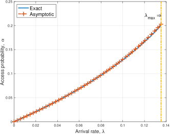
Figure 5: The access probability, $\alpha$, as a function of $\lambda$ when $N=40$ and $L=20$.

Note that since ${\mathbb{W}}_{0}(-x)\in[-1,0]$ for $x\in[0,e^{-1}]$ and $\alpha\leq 1$, it can be confirmed that

$$\tilde{\alpha}_{\rm max}\leq\frac{1}{\eta}=\frac{L}{N}.$$ (22)

In (8), $G$ is usually called the throughput that can be maximized when the access probability, $\alpha$, is $\frac{L}{N}$, which is also shown in Fig. 4, where $S(\alpha)=\frac{G}{N}$ (in this sense, $S$ can be seen as the normalized throughput per device). In conventional multichannel ALOHA (i.e., non-buffered multichannel ALOHA), the system is known to be stable if $\alpha<\frac{L}{N}$ [35], while multichannel ALOHA with fast retrial is stable if $\alpha<\alpha_{\rm max}$. Note that due to the presence of buffers at devices, multichannel ALOHA with fast retrial is also buffered multichannel ALOHA as mentioned earlier. In Fig. 6, the maximum throughput of conventional multichannel ALOHA, which is $\max G=N\bar{S}$, is shown with that of (buffered) multichannel ALOHA with fast trial for different numbers of devices, $N$, when $L=20$. Since $\max G=N\bar{S}\approx Le^{-1}$, the maximum throughput of conventional multichannel ALOHA is almost independent of $N$. On the other hand, the maximum throughput of multichannel ALOHA with fast trial, $NS(1)=N\left(1-\frac{1}{L}\right)^{N-1}$, decreases with $N$. Clearly, when fast retrial is employed for low access delay, it is necessary to keep the number of devices small.

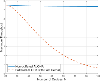
Figure 6: Maximum throughput of conventional multichannel ALOHA and that of multichannel ALOHA with fast retrial as functions of $N$ when $L=20$.

In addition, there are few remarks as follows.

• In [21], a steady-state analysis can be found under the assumption that the number of retrials follows a Poisson distribution. Although this assumption simplifies the analysis, it is not valid (as stated in [21]). In this paper, fortunately, no assumption about the distribution of retrials is required.

• In [26], as will be discussed in the next section (i.e., Section IV) the notion of effective bandwidth is applied to multichannel ALOHA with a number of assumptions that simplify analysis. Among those, in this paper, two assumptions (in particular, the assumptions of A1 and A2 in [26]) are not used, while one assumption (or approximation) of independent departures is still used (to find the distribution of $K$ in (11)). Thus, the results in this paper are still approximate, although they are reasonably close to simulation results as will be shown in Section V.

IV QoS Exponent in Steady-State

In this section, we exploit the notion of effective bandwidth [27] [28] [36] to find the tail distribution of queue length in steady-state.

IV-A Effective Bandwidth and QoS Exponent

Consider the logarithm of moment generating functions (LMGFs) of $a_{n}(t)$ and $s_{n}(t)$ that are given by

$$\Lambda_{a}(\theta) =\ln{\mathbb{E}}[e^{\theta a_{n}}]$$ (23)

$$\Lambda_{s}(\theta) =\ln{\mathbb{E}}[e^{\theta s_{n}}].$$ (24)

From (2), we can also show that

$$\Lambda_{s}(\theta)=\ln\left(1-p+pe^{\theta}\right),$$ (25)

where $p$ is the probability of successful transmission without collision.

In this section, we assume that $a_{n}(t)$ is an independent Poisson arrival with mean $\lambda$ for all $n$. Thus, we have $\Lambda_{a}(\theta)=\lambda(e^{\theta}-1)$. In this case, we can find a relation between the probability of empty queue, i.e., $\Pr(q_{n}=0)$, and the access probability as follows.

Lemma 3

Under the assumption that $a_{n}(t)$ is Poisson, the access probability, $\alpha$, is given by

$$\alpha=1-e^{-\lambda}\Pr(q_{n}=0).$$ (26)

Proof:

The transmission probability or access probability is the probability that a device has a packet to transmit. A device has a packet to transmit if the queue is not empty or if there are any arrivals when the queue is empty. Thus, it can be shown that

$$\alpha =\Pr(q_{n}\geq 1)+\Pr(a_{n}\geq 1\,|\,q_{n}=0)\Pr(q_{n}=0)$$ (27)

$$=\Pr(q_{n}\geq 1)+\Pr(a_{n}\geq 1)\Pr(q_{n}=0)$$ (28)

$$=(1-\Pr(q_{n}=0))+(1-e^{-\lambda})\Pr(q_{n}=0),$$ (29)

which leads to (26). ∎

According to [27] [28], in steady-state, the queue length has the following tail probability:

$$\Pr(q_{n}(\infty)\geq\tau)\buildrel\cdot\over{=}e^{-\theta^{*}\tau},\ \tau>0,$$ (30)

where $\theta^{*}>0$ is the solution of the following equation:

$$\Lambda_{a}(\theta)+\Lambda_{s}(-\theta)=0.$$ (31)

In (30) for two functions $f(x)$ and $g(x)$, we say that $f(x)\buildrel\cdot\over{=}g(x)$ if $\lim_{x\to\infty}\frac{1}{x}\ln\frac{f(x)}{g(x)}=0$, i.e., the two functions are asymptotically equal to the first order in the exponent.

To find $\theta^{*}$, we need to know $p$. Consider device $n$. Under the symmetric condition in (10), $p=\Pr(s_{n}=1)$ for all $n$. In fact, $s_{n}$ depends on the states of the other devices’ queues. For convenience, let $K_{-n}$ denote the number of the other devices that transmit. Clearly, we have $s_{n}=1$ only when all the other $K_{-n}$ devices choose different preambles. That is,

$$\Pr(s_{n}=1\,|\,K_{-n}=k)=\left(1-\frac{1}{L}\right)^{k}.$$ (32)

As mentioned earlier, if (4) holds, each queue has a stationary distribution. Thus, with $\alpha$, the probability that there are the other $k$ active devices is given by

$$\Pr(K_{-n}=k)=\binom{N-1}{k}\alpha^{k}(1-\alpha)^{N-1-k}.$$ (33)

After some manipulations, $p$ can be found as

$$p =\Pr(s_{n}=1)$$ (34)

$$=\sum_{k=0}^{N-1}\Pr(s_{n}=1\,|\,K_{-n}=k)\Pr(K_{-n}=k)$$ (35)

$$=\sum_{k=0}^{N-1}\left(1-\frac{1}{L}\right)^{k}\binom{N-1}{k}\alpha^{k}(1-\alpha)^{N-1-k}$$ (36)

$$=\left(1-\frac{\alpha}{L}\right)^{N-1}.$$ (37)

Lemma 4

Suppose that $N\to\infty$ with a fixed ratio $\eta=\frac{N}{L}$. Then, $p$ converges to a constant that is given by

$$\tilde{p}=\lim_{N\to\infty}p=e^{-\tilde{\alpha}\eta}=\exp({\mathbb{W}}_{0}(-\lambda\eta)).$$ (38)

Proof:

According to Lemma 2, $\alpha$ converges to $\tilde{\alpha}$ as $N\to\infty$. Thus, we can readily have (38). ∎

In Fig. 7, $p$ is shown as a function of $\lambda$ with its asymptotic, $\tilde{p}$, in (38) when $N=40$ and $L=20$. The difference between $p$ and $\tilde{p}$ is not significant if $\lambda$ is not close to $\lambda_{\rm max}$.

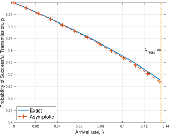
Figure 7: The probability of successful transmission, $p$, when $N\geq L$, as a function $\lambda$ with its asymptotic, $\tilde{p}$ when $N=40$ and $L=20$.

Consequently, for a given $\lambda$, from (12), $\alpha$ can be obtained, and then finally, $p$ can be found from $\alpha$ using (37), which is illustrated as follows:

$$\lambda\to\alpha\ (\mbox{via \eqref{EQ:ll}})\to p\ (\mbox{via \eqref{EQ:p_a}}).$$

Once $p$ is obtained, we can substitute it into (31) to find $\theta^{*}$, which is the solution of the following equality from (31):

$$\lambda(e^{\theta}-1)+\ln\left(1-p(1-e^{-\theta})\right)=0.$$ (39)

As a result, the asymptotic distribution of queue length in (30) can be found, which allows us to understand access delay through (30).

It is also possible to set a target QoS exponent for certain guaranteed access delay. For example, if the probability of more than or equal to $\tau=3$ fast retrials has to be less than or equal to $0.01$, we can have

$$\theta^{*}=-\frac{\ln(0.01)}{\tau}=1.5351.$$ (40)

Then, for a given number of devices, $N$, key parameters such as $\lambda$ and $L$ can be decided to keep $\theta^{*}\geq 1.5351$. On the other hand, if $\lambda$ and $L$ are fixed, the number of devices, $N$, can be limited to keep QoS in terms of the QoS exponent as part of admission control.

IV-B Bounds on QoS Exponent and Existence of a Positive $\theta^{*}$

In [26], with known $p$, bounds on $\theta^{*}$ are found as

$$\theta_{\rm L}\leq\theta^{*}\leq\theta_{\rm U},$$ (41)

where

$$\theta_{\rm U}=\ln\left(1-\frac{\ln(1-p)}{\lambda}\right)\ \mbox{and}\ \theta_{\rm L}=\ln\frac{p}{\lambda}.$$ (42)

In addition, it is shown that the solution of $\theta>0$ that satisfies (39) is unique if exists. A sufficient condition that a positive solution, i.e., $\theta^{*}>0$, exists is simply $p>\lambda$, because the lower bound, $\theta_{\rm L}$, in (42) becomes positive if $p>\lambda$.

Lemma 5

Suppose that $N\to\infty$ with a fixed ratio $\eta=\frac{N}{L}\geq 1$. Then, if $\lambda<\lambda_{\rm max}$, $\tilde{p}>\lambda$.

Proof:

From (19) and the properties of Lambert W function [34], it can be shown that

$$\tilde{p}=\exp\left({\mathbb{W}}_{0}(-\lambda\eta)\right)=\frac{\lambda\eta}{-{\mathbb{W}}_{0}(-\lambda\eta)}.$$ (43)

Thus, $\tilde{p}>\lambda$ is equivalent to the following:

$$\eta>-{\mathbb{W}}_{0}(-\lambda\eta).$$ (44)

Since $\lim_{N\to\infty}\lambda_{\rm max}=e^{-\eta}$, we have $\lambda\eta<\eta e^{-\eta}$ when $N\to\infty$, which implies that

$$-{\mathbb{W}}_{0}(-\lambda\eta)<-{\mathbb{W}}_{0}(-\eta e^{-\eta})\leq-{\mathbb{W}}_{0}(-e^{-1})=1.$$ (45)

Since $\eta=\frac{N}{L}\geq 1$, (44) holds, which completes the proof. ∎

According to Lemma 5, we can see that $\theta^{*}>0$ exists if $\lambda<\lambda_{\rm max}$. In other words, the stability condition in (4) results in a positive QoS exponent in large systems (i.e., when $N\to\infty$ with a fixed ratio $\eta$).

V Simulation Results

In this section, we present simulation results with independent Poisson arrivals for $a_{n}(t)$, i.e., $a_{n}(t)\sim{\rm Pois}(\lambda)$ for all $n=1,\ldots,N$. In order to find the distribution of queue length, the state of queue is obtained for $t\in\{1,\ldots,T\}$ with $q_{n}(0)=0$, where $T=4000$ is the number of slots in each run. To obtain the steady-state results, we only use the last 2000 states in each run. Furthermore, each simulation result is an average obtained from 1000 independent runs. To compare with simulation results, the tail distribution in (30) is used as an analytical result with $\theta^{*}$ that is obtained using $\tilde{p}$ for given $\lambda$ and $\eta$ using (38), since the asymptotic results are reasonably accurate with not too large $N$ and $L$ (as shown in Figs. 5 and 7).

Fig. 8 shows the tail distribution of queue length, $\Pr(q_{n}\geq\tau)$ as a function of arrival rate, $\lambda$, with $\tau\in\{1,\ldots,4\}$ when $\eta=2$. In this case, $\lambda_{\rm max}=(1-\frac{1}{L})^{N-1}\approx e^{-\eta}=0.1353$. It is clear that the analytical results are close to simulation results although (30) is used for a large $\tau$. This demonstrates that the analytical approach derived in this paper can be used to design a 2-step approach with fast retrial when access delay constraints are imposed with certain target QoS exponents or tail probabilities. For example, to satisfy $\Pr(q_{n}\geq 3)\leq 10^{-4}$, we can see that $\lambda$ has to be less than or equal to $0.08$ according to Fig. 8.

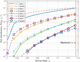
(a)

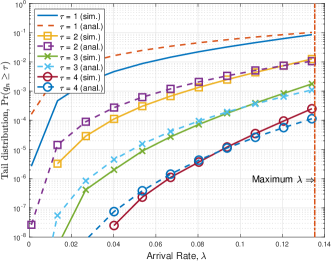
(b)

Figure 8: Tail distribution of queue length, $\Pr(q_{n}\geq\tau)$ as a function of arrival rate, $\lambda$, with $\tau\in\{1,\ldots,4\}$ when $\eta=2$: (a) $N=50$ and $L=25$; (b) $N=100$ and $L=50$.

In this paper, an approximation that the departures are independent is used to find the distribution of $K$ in (11). For Poisson arrivals, we have found the relation between $\Pr(q_{n}=0)$ and $\alpha$ in (26). From simulations, we obtain the probability of empty queue, i.e., $\Pr(q_{n}=0)$, and from this, a simulation result of $\alpha$ is found using (26) for comparison with $\alpha$ obtained by solving (12), which is referred to as “theory” in Fig. 9. It is clearly shown that the approximation of independent departures is reasonable to find $\alpha$ as it closely matches simulation results (especially when $\lambda$ is small).

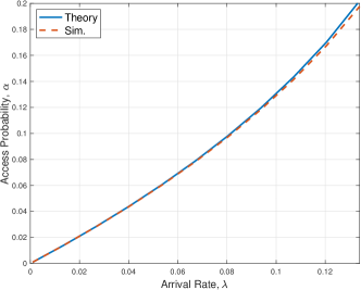
Figure 9: The access probability, $\alpha$, as a function of arrival rate, $\lambda$ when $N=50$ and $L=25$.

In Fig. 10, we show the tail distribution of queue length, $\Pr(q_{n}\geq\tau)$ as a function of the number of devices, $N$, with $\tau\in\{1,\ldots,4\}$ when $\lambda=0.15$. In general, we can see that the tail probability increases with $N$ for a fixed $L$. Furthermore, the analytical results agree with simulation results when the system is large (e.g., the analytical results with $L=60$ (in Fig. 10 (b)) are closer to the simulation results than that with $L=10$ (in Fig. 10 (a)).

It is noteworthy that for given $L$ and $\lambda$, according to (4), the maximum of $N$ for a stable system, is $N_{\rm max}=1+\frac{\ln\lambda}{\ln(1-(1/L))}$. In other words, if $N>N_{\rm max}$, no stability is guaranteed according to (4). However, as shown in in Fig. 10, although $N$ is greater than $N_{\rm max}$, the tail probability can be low. As mentioned earlier, since (4) is a sufficient condition, there can be $N>N_{\rm max}$ with stable queues. Thus, we need to have a sufficient and necessary condition, which will be a further issue to be studied in the future.

Furthermore, it can be observed that with a small system (i.e., $L=10$ in Fig. 10 (a)), the tail probability from (30) does not predict simulation results well when $N$ is close to $N_{\rm max}$. This mainly results from the independent departure approximation used in (11), which is generally reasonable for a large system [23] [26]. This can be confirmed by Fig. 10 (b), where $L$ is larger than that in Fig. 10 (a) by a factor of $10$, as the tail probability from (30) is reasonably close to the simulation results when $N\to N_{\rm max}$.

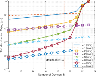
(a)

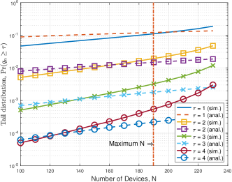
(b)

Figure 10: Tail distribution of queue length, $\Pr(q_{n}\geq\tau)$ as a function of the number of devices, $N$, with $\tau\in\{1,\ldots,4\}$ when $\lambda=0.15$: (a) $L=10$; (b) $L=100$.

Fig. 11 shows the tail distribution of queue length, $\Pr(q_{n}\geq\tau)$ as a function of the number of preambles, $L$, with $\tau\in\{1,\ldots,4\}$ when $N=50$ and $\lambda\in\{0.075,0.15\}$. It is shown that the tail probability decreases with $L$ when $N$ is fixed. Note that the minimum of $L$ according to (4) is given by $L_{\rm min}=(1-\lambda^{\frac{1}{N-1}})^{-1}$. However, although $L<L_{\rm min}$, the tail probability is low according to simulation results, which confirms again that (4) is a sufficient condition for stable systems.

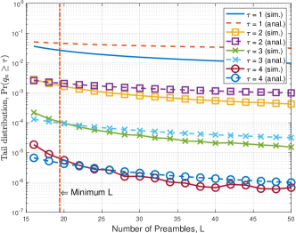
(a)

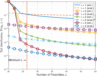
(b)

Figure 11: Tail distribution of queue length, $\Pr(q_{n}\geq\tau)$ as a function of the number of preambles, $L$, with $\tau\in\{1,\ldots,4\}$ when $N=50$: (a) $\lambda=0.075$; (b) $\lambda=0.15$.

To see the impact of the size of the system on the performance, we consider a scaling factor, denoted by $s$, for a baseline system with $(N_{0},L_{0})=(20,10)$. With a fixed $\eta=2$, the system size increases with $s$, i.e., $N=N_{0}s$ and $L=L_{0}s$. The results are shown in Fig. 12 when $\lambda=0.1$, which demonstrates that the tail probability is almost invariant with respect to the scaling factor. Thus, it confirms that the asymptotic analysis can be used to understand 2-step approaches (with large $L$ and $N$) based on multichannel ALOHA with fast retrial.

Figure 12: Tail distribution of queue length, $\Pr(q_{n}\geq\tau)$ as a function of the scaling factor, denoted by $s$, with $\tau\in\{1,\ldots,4\}$ when $(N,L)=(N_{0}s,L_{0}s)$ and $\lambda=0.1$. Here, $(N_{0},L_{0})=(20,10)$ for the baseline system.

VI Concluding Remarks

In this paper, we studied 2-step random access approaches with fast retrial in MTC for delay-sensitive or real-time IoT applications, since they can have low access delay. Under a sufficient condition for stable systems, we performed steady-state analysis so that the probability of successful transmission can be analytically obtained for given parameters such as the mean arrival rate and the numbers of devices and preambles. Since the derived approach in this paper required less assumptions or approximations than [26], it was able to provide a better approximation of QoS exponent, which was confirmed by simulation results.

Based on the results in this paper, there are a number of topics to be further investigated. For example, in the case that delay-sensitive and delay-tolerant devices co-exist, optimal resource allocation is required. The derived analytical approach in this paper can be used for optimization to meet target QoS exponents for delay-sensitive devices. It is also important to improve the derived approach in this paper for a better approximation of QoS exponent and generalize to the case that devices have different arrival rates.

References

- [1] J. Gubbi, R. Buyya, S. Marusic, and M. Palaniswami, “Internet of Things (IoT): A vision, architectural elements, and future directions,” Future Gener. Comput. Syst., vol. 29, pp. 1645–1660, Sept. 2013.
- [2] A. Al-Fuqaha, M. Guizani, M. Mohammadi, M. Aledhari, and M. Ayyash, “Internet of Things: A survey on enabling technologies, protocols, and applications,” IEEE Communications Surveys Tutorials, vol. 17, pp. 2347–2376, Fourthquarter 2015.
- [3] R. Buyya and A. V. Dastjerdi, Internet of Things: Principles and Paradigms. San Francisco, CA, USA: Morgan Kaufmann Publishers Inc., 1st ed., 2016.
- [4] Q. M. Qadir, T. A. Rashid, N. K. Al-Salihi, B. Ismael, A. A. Kist, and Z. Zhang, “Low power wide area networks: A survey of enabling technologies, applications and interoperability needs,” IEEE Access, vol. 6, pp. 77454–77473, 2018.
- [5] J. Famaey, R. Berkvens, G. Ergeerts, E. D. Poorter, F. V. d. Abeele, T. Bolckmans, J. Hoebeke, and M. Weyn, “Flexible multimodal sub-gigahertz communication for heterogeneous Internet of Things applications,” IEEE Communications Magazine, vol. 56, no. 7, pp. 146–153, 2018.
- [6] J. Ding, M. Nemati, C. Ranaweera, and J. Choi, “IoT connectivity technologies and applications: A survey,” IEEE Access, vol. 8, pp. 67646–67673, 2020.
- [7] C. Bockelmann, N. Pratas, H. Nikopour, K. Au, T. Svensson, C. Stefanovic, P. Popovski, and A. Dekorsy, “Massive machine-type communications in 5G: physical and MAC-layer solutions,” IEEE Communications Magazine, vol. 54, pp. 59–65, Sep 2016.
- [8] M. Bennis, M. Debbah, and H. V. Poor, “Ultrareliable and low-latency wireless communication: Tail, risk, and scale,” Proceedings of the IEEE, vol. 106, pp. 1834–1853, Oct 2018.
- [9] P. Popovski, C. Stefanovic, J. J. Nielsen, E. de Carvalho, M. Angjelichinoski, K. F. Trillingsgaard, and A. Bana, “Wireless access in ultra-reliable low-latency communication (URLLC),” IEEE Trans. Communications, vol. 67, pp. 5783–5801, Aug 2019.
- [10] 3GPP TR 37.868 V11.0, Study on RAN improvments for machine-type communications, October 2011.
- [11] 3GPP TS 36.321 V13.2.0, Evolved Universal Terrestrial Radio Access (E-UTRA); Medium Access Control (MAC) protocol specification, June 2016.
- [12] C. Bockelmann, N. K. Pratas, G. Wunder, S. Saur, M. Navarro, D. Gregoratti, G. Vivier, E. De Carvalho, Y. Ji, C. Stefanović, P. Popovski, Q. Wang, M. Schellmann, E. Kosmatos, P. Demestichas, M. Raceala-Motoc, P. Jung, S. Stanczak, and A. Dekorsy, “Towards massive connectivity support for scalable mMTC communications in 5G networks,” IEEE Access, vol. 6, pp. 28969–28992, 2018.
- [13] G. Wunder, P. Jung, and C. Wang, “Compressive random access for post-LTE systems,” in Proc. IEEE ICC, pp. 539–544, June 2014.
- [14] G. Wunder, C. Stefanovi, P. Popovski, and L. Thiele, “Compressive coded random access for massive MTC traffic in 5G systems,” in 2015 49th Asilomar Conference on Signals, Systems and Computers, pp. 13–17, Nov 2015.
- [15] J. Choi, “Two-stage multiple access for many devices of unique identifications over frequency-selective fading channels,” IEEE Internet of Things J., vol. 4, pp. 162–171, Feb 2017.
- [16] J. Choi, “On throughput of compressive random access for one short message delivery in IoT,” IEEE Internet of Things J., vol. 7, no. 4, pp. 3499–3508, 2020.
- [17] A. T. Abebe and C. G. Kang, “Comprehensive grant-free random access for massive low latency communication,” in 2017 IEEE International Conference on Communications (ICC), pp. 1–6, May 2017.
- [18] K. Senel and E. G. Larsson, “Grant-free massive MTC-enabled massive MIMO: A compressive sensing approach,” IEEE Trans. Communications, vol. 66, pp. 6164–6175, Dec 2018.
- [19] L. Liu, E. G. Larsson, W. Yu, P. Popovski, C. Stefanovic, and E. de Carvalho, “Sparse signal processing for grant-free massive connectivity: A future paradigm for random access protocols in the Internet of Things,” IEEE Signal Processing Magazine, vol. 35, pp. 88–99, Sept 2018.
- [20] J. Ding, D. Qu, and J. Choi, “Analysis of non-orthogonal sequences for grant-free RA with massive MIMO,” IEEE Trans. Communications, vol. 68, pp. 150–160, Jan 2020.
- [21] Y.-J. Choi, S. Park, and S. Bahk, “Multichannel random access in OFDMA wireless networks,” IEEE J. Selected Areas in Communications, vol. 24, pp. 603–613, March 2006.
- [22] A. Mutairi, S. Roy, and G. Hwang, “Delay analysis of OFDMA-aloha,” IEEE Trans. Wireless Communications, vol. 12, pp. 89–99, January 2013.
- [23] L. Dai, “Stability and delay analysis of buffered aloha networks,” IEEE Trans. Wireless Communications, vol. 11, pp. 2707–2719, August 2012.
- [24] W. Zhan and L. Dai, “Massive random access of machine-to-machine communications in LTE networks: Modeling and throughput optimization,” IEEE Trans. Wireless Communications, vol. 17, no. 4, pp. 2771–2785, 2018.
- [25] C. Zhang, X. Sun, J. Zhang, X. Wang, S. Jin, and H. Zhu, “Throughput optimization with delay guarantee for massive random access of M2M communications in industrial IoT,” IEEE Internet of Things J., vol. 6, no. 6, pp. 10077–10092, 2019.
- [26] J. Choi, “Low-latency multichannel ALOHA with fast retrial for machine-type communications,” IEEE Internet of Things J., vol. 6, pp. 3175–3185, April 2019.
- [27] C.-S. Chang and J. A. Thomas, “Effective bandwidth in high-speed digital networks,” IEEE J. Selected Areas Commun., vol. 13, pp. 1091–1100, Aug. 1995.
- [28] D. Wu and R. Negi, “Effective capacity: a wireless link model for support of quality of service,” IEEE Trans. Wireless Commun., vol. 2, pp. 630–643, July 2003.
- [29] J. Norris, Markov Chains. Cambridge Series in Statistical and Probabilistic Mathematics, Cambridge University Press, 1998.
- [30] J. Choi, “On the stability of fast retrial multichannel ALOHA with rate control for MTC,” IEEE Communications Letters, vol. 22, pp. 360–363, Feb 2018.
- [31] J. Choi, “Fast retrial for low-latency connectivity in MTC with two different types of devices,” IEEE Wireless Communications Letters, pp. 1–4, 2020 (accepted).
- [32] F. Kelly and E. Yudovina, Stochastic Networks. Cambridge University Press, 2014.
- [33] B. Hajek, Random Processes for Engineers. Cambridge University Press, 2015.
- [34] R. Corless, G. Gonnet, D. Hare, D. Jeffrey, and D. Knuth, “On the lambert W function,” Advances in Computational Mathematics, vol. 5, no. 1, pp. 329–359, 1996.
- [35] D. Shen and V. O. K. Li, “Performance analysis for a stabilized multi-channel slotted ALOHA algorithm,” in Proc. IEEE PIMRC, vol. 1, pp. 249–253 Vol.1, Sept 2003.
- [36] F. Kelly, S. Zachary, and I. Ziedins, Stochastic Networks: Theory and Applications. Oxford University Press, 1996.