Exact Properties of SIQR model for COVID-19

Abstract

The SIQR model is reformulated where compartments for infected and quarantined are redefined so as to be appropriate to COVID-19, and exact properties of the model are presented. It is shown that the maximum number of infected at large depends strongly on the quarantine rate and that the quarantine measure is more effective than the lockdown measure in controlling the pandemic. The peak of the number of quarantined patients is shown to appear some time later than the time that the number of infected becomes maximum. On the basis of the expected utility theory, a theoretical framework to find out an optimum strategy in the space of lockdown measure and quarantine measure is proposed for minimizing the maximum number of infected and for controlling the outbreak of pandemic at its early stage.

1 Introduction

Since November 2019, the pandemic COVID-19 is still expanding in the world, infected of which totals more than 15 million at 22 nd of July, 2020[1]. It is an important problem of socio-physics to construct a simple model by which one can understand the nature of the outbreak, and to construct a theoretical framework for formulating the optimum strategy to control it.[2]

Epidemics can be considered to be a problem of physics concerning reaction and relaxation processes and the simplest understanding of its outbreak can be provided by a mean field analysis. The SIR model[3] assumes three compartments (or species) in population, susceptible (S), infected (I) and removed (R), and the infection is transferried from an infected individual to a susceptible individual. The number of symptomatic patients, which is identical to the number of infected, decreases in the community by treatment and/or quarantine. The SIR model is considered a standard model to explain the infection trajectory of ordinary epidemics like influenza.

COVID-19 has unusual characteristics: (1) transmission of the virus by presymptomatic patients and (2) existence of asymptomatic infectious patients, and (3) patients, symptomatic or asymptomatic, can be identified by PCR test. Because of these characteristics, the number of infected cannot be obtained directly and the number of daily confirmed new cases and its time dependence are the only essential observables. Therefore, COVID-19 showing these characteristics may not be represented properly by the SIR and the SEIR models which assume that the number of patients is known and do not treat quarantined patients as a compartment.

The SIQR model [5, 6] is a compartmental model which represents a community by four compartments, assuming an additional compartment of quarantined (Q), and describes the transmission process by a system of ordinary nonlinear differential equations. The SIQR model seems to be appropriate to COVID-19 and it has been successfully applied in the analysis of the early stage of the outbreak of COVID-19 in Italy[7], India[8, 9], Sweden[10] and Japan[11].

In this paper, I redefine the SIQR model so as to make it appropriate to COVID-19[11]. Namely, I classify patients into two groups; (1) infected patients at large (I) who can be in any of three states, presymptomatic, symptomatic and asymptomatic and (2) quarantined patients (Q) who are in a hospital or self-isolated at home and no longer infectious in the community. I treat the number of daily confirmed new cases explicitly and consider the quarantine rate or the fraction of infected at large put in a quarantine or self-isolation as a key parameter which can be determined from the observation of the daily confirmed new cases. I also discuss the optimum strategy for controlling the pandemic.

This paper is organized as follows. First, I explain in Sec. 2 the SIQR model and discuss its relevancy to COVID-19. I also present the basic properties of the model, showing parameter dependence of the maximum number of infected. Section 3 considers the exact solution of the SIQR model and shows the time dependence of various quantities including the number of quarantined. A theoretical frame work for optimizing measures to control the outbreak is discussed in Sec. 4, where the expected utility theory[12] is exploited. The frame work is applied for optimizing strategy for reducing the epidemic peak and for stamping out the epidemic as fast as possible. Results are discussed in Sec. 5.

2 SIQR model and basic properties

2.1 Model

The basic concept of the SIQR model is identical to the chemical reaction, which can be described by rate equations. The dynamics of the SIQR model is given by the following set of ordinary nonlinear differential equations:

$$\frac{dx}{dt} = -\beta x(t)y(t),$$ (1)

$$\frac{dy}{dt} = \beta x(t)y(t)-qy(t)-\gamma y(t),$$ (2)

$$\frac{dw}{dt} = qy(t)-\gamma^{\prime}w(t),$$ (3)

$$\frac{dz}{dt} = \gamma y(t)+\gamma^{\prime}w(t),$$ (4)

where $t$ is the time, and $x(t)$, $y(t)$, $w(t)$ and $z(t)$ are the fractions of population ($N$) in each compartment, susceptible, infected at large, quarantined patients and recovered (and died) patients. Here, I assumed that new patients immediately after they get infected cannot be quarantined since the incubation period is long for COVID-19. The parameters of this model are a transmission coefficient $\beta$, quarantine rate of infected at large $q$, and recovery rates $\gamma$ and $\gamma^{\prime}$ of infected at large and quarantined, respectively. These parameters can be estimated from observations; $\beta$, $\gamma$ and $\gamma^{\prime}$ from epidemiological survey and $q$ from the time dependence of the daily confirmed new cases. Although time can be scaled by one of parametes, I use one day as a unit of time in this paper so that ordinary citizens and policy makers can understand results without difficulties.

Infected at large, regardless whether they are symptomatic or asymptomatic, are quarantined at a per capita rate $q$ and become non-infectious in the community. Quarantined patients recover at a per capita rate $\gamma^{\prime}$ (where $1/\gamma^{\prime}$ is the average time it takes for recovery) and infected at large become non-infectious at a per capita rate $\gamma$ (where $1/\gamma$ is the average time that an infected patient at large is capable of infecting others). It is apparent that Eqs. (1) $\sim$ (4) guaranteee the conservation of population $x(t)+y(t)+w(t)+z(t)=1$.

If one considers quarantined and recoverd together as removed, the set of differential equation is the same as the set of equations for the SIR model with removal rate of infected $q+\gamma$. Since the value of $q$ depends strongly on government policies and the only observable is the number of quarantined patients $\Delta w(t)=qy(t)$ on each day, it is important to treat the quarantined and recovered patients separately in the analysis of the outbreak of COVID-19.

Figure 1 shows the elementary processes of the SIQR model.

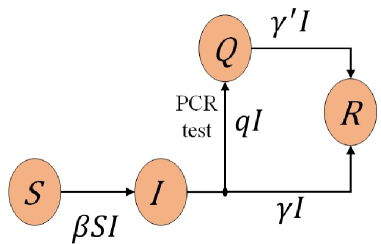
Figure 1: Elementary processes of the SIQR model. $x$ and $y$ obey a reaction $x+y\rightarrow 2y$.

2.2 Basic properties

From Eqs. (1) and (2), it is easy to show that the trajectory in the $(x,y)$ plane is determined by

$$\frac{dy}{dx}=\frac{q+\gamma}{\beta x}-1.$$ (5)

Therefore, the trajectory in the $(x,y)$ plane is given by

$$y=1-x+\frac{q+\gamma}{\beta}\ln x,$$ (6)

where the initial condition is set to $y=0$ at $x=1$. Figure 2 shows the trajectories (a) for various $\beta$ at $q=0.1$ and (b) for various $q$ at $\beta=0.4$ when $\gamma=0.06$.

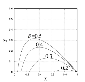
(a)                                                             (b)

Figure 2: Trajectories in the $(x,y)$ plane. (a) for various $\beta$ when $q=0.1$ and (b) for various $q$ when $\beta=0.4$, where $\gamma=0.06$.

The peak position $(x^{*},y^{*})$ of the trajectory can be obtained from Eqs. (5) and (6) by setting $\frac{dy}{dx}=0$. I find that

$$x^{*} = \frac{q+\gamma}{\beta},$$ (7)

$$y^{*} = 1-\frac{q+\gamma}{\beta}+\frac{q+\gamma}{\beta}\ln\frac{q+\gamma}{\beta}.$$ (8)

Figure 3 shows the dependence of $y^{*}$ on $\beta$ and $q$: (a) three dimensional plot of $y^{*}(\beta,q)$, (b) the $\beta$ dependence at $q=0.1$ and (c) the $q$ dependence at $\beta=0.4$ when $\gamma=0.06$. The peak height becomes lower for smaller $\beta$ and enhanced $q$, and the latter is more effective in reducing the peak.

(a)

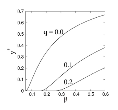
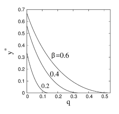
(b)                                                              (c)

Figure 3: Peak heights of infected at large as a function of $\beta$ and $q$. (a) Three dimensional plot, (b) for various $q$ when $\beta=0.4$ and (c) for various $\beta$ when $q=0.1$, where $\gamma=0.06$.

3 Time dependence of the outbreak

3.1 Exact properties

Combining Eqs. (3) and (4) together, I obtain

$$\frac{d(w+z)}{dt}=(q+\gamma)y(t).$$ (9)

Therefore, the set of Eqs. (1), (2) and (9) is identical to the basic equations of the SIR model as stated before, and the exact solution can be written as[13]

$$x(t) = x_{0}u(t),$$ (10)

$$y(t) = 1-x_{0}u(t)+\frac{q+\gamma}{\beta}\ln u(t),$$ (11)

$$w(t)+z(t) = -\frac{q+\gamma}{\beta}\ln u(t),$$ (12)

where time $t$ is related to $u$ through an integral

$$t=\int_{1}^{u}\frac{d\xi}{\xi[x_{0}\beta\xi-\beta-(q+\gamma)\ln\xi]}.$$ (13)

Once $y(t)$ is known, then $w(t)$ is obtained from Eq. (3),

$$w(t)=qe^{-\gamma^{\prime}t}\int_{0}^{t}e^{\gamma^{\prime}t^{\prime}}y(t^{\prime})dt^{\prime},$$ (14)

and thus $z(t)$ is given by

$$z(t)=-\frac{q+\gamma}{\beta}\ln u(t)-qe^{-\gamma^{\prime}t}\int_{0}^{t}e^{\gamma^{\prime}t^{\prime}}y(t^{\prime})dt^{\prime}.$$ (15)

Figure 4 shows the time dependence of $x(t)$, $y(t)$, $w(t)$ and $z(t)$ for $\beta=0.4$, $q=0.1$ and $\gamma=\gamma^{\prime}=0.06$. It is interesting to note that the number of quarantined patients $w(t)$ takes its maximum at some time later than the time that the number of infected $y(t)$ becomes maximum.

Figure 4: The exact time dependence of $x(t)$, $y(t)$, $w(t)$ and $z(t)$ when $\beta=0.4$, $q=0.1$ and $\gamma=\gamma^{\prime}=0.06$. The peak positions of $y(t)$ and $w(t)$ differ about 10 days for the choice of parameters.

The observable in COVID-19 is the daily confirmed new cases $\Delta w(t)=qy(t)$, which is simply $q$-times smaller than $y(t)$ as shown in Fig. 5.

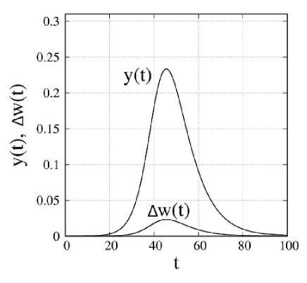
Figure 5: The time dependence of $y(t)$ and $\Delta w(t)$ for $\beta=0.4$, $q=0.1$ and $\gamma=\gamma^{\prime}=0.06$.

3.2 Properties at the early stage of outbreak

Since $x(t)\simeq x_{0}$ and $y_{0}\simeq 0$ in the early stage of outbreak, I introduce a new integration variable $\eta=1-\xi$ in Eq. (13)

$$t=-\int_{0}^{1-u}\frac{d\eta}{(1-\eta)[x_{0}\beta(1-\eta)-\beta-(q+\gamma)\ln(1-\eta)]}.$$ (16)

Taking up to the first order term in $1-u$ in the integrand on the right-hand side of Eq. (16) and up to the first order term in $y_{0}$, I obtain

$$u(t)=1+\frac{y_{0}\beta}{q+\gamma-\beta}\left(e^{(\beta-q-\gamma)t}-1\right).$$ (17)

Therefore, the short-term solution of the SIQR model is given by

$$x(t) = x_{0}-\frac{y_{0}\beta}{\beta-q-\gamma}\left(e^{(\beta-q-\gamma)t}-1\right),$$ (18)

$$y(t) = y_{0}e^{(\beta-q-\gamma)t},$$ (19)

$$w(t) = \frac{y_{0}q}{\beta-q-\gamma+\gamma^{\prime}}\left(e^{(\beta-q-\gamma)t}-e^{-\gamma^{\prime}t}\right),$$ (20)

$$z(t) = \frac{y_{0}(q+\gamma)}{\beta-q-\gamma}\left(e^{(\beta-q-\gamma)t}-1\right)-\frac{y_{0}q}{\beta-q-\gamma+\gamma^{\prime}}\left(e^{(\beta-q-\gamma)t}-e^{-\gamma^{\prime}t}\right).$$ (21)

These solution can also be obtained by setting $x(t)=x_{0}=1$ in Eqs. (1) $\sim$ (4) and have been used in the analysis of the outbreak of COVID-19 [7, 8, 9, 11].

The short-term solution indicates that the initial growth rate of the number of infected at large is determined by

$$\lambda=\beta-q-\gamma.$$ (22)

In order to control the outbreak, a measure must be formulated to make the growth rate $\lambda$ negative under various restrictions in economic activities and medical care systems.

4 Optimum measure

4.1 General frame work

As shown in Fig. 4, the present model like the SIR model shows that the epidemic curve will converge to an equilibrium state after several months, passing a maximum number of infected which could be $15\sim 25$ % of population depending on the value of parameters. This means that if we wait the natural epidemic equilibrium, the number of causalities will become unacceptably large. In order to reduce the number of causalities, all governments in the world have been struggling against COVID-19 with various measures. Lockdown and social distancing are measures to reduce the effective transmission coefficient $\beta$, but it has a severe damage on economic activities. For COVID-19, quarantine measure including self-isolation has been employed in many countries to increase the quarantine rate $q$.

Since $\gamma$ in the SIQR model cannot be altered, $\beta$ and $q$ are the essential parameters which can be modified by policy. I parameterize $\beta$ as $\beta=(1-a)\beta_{0}$ where $a$ represents the strength of lockdown measure; $a=0$ corresponds to no measure on social distancing and $a=1$ denotes complete lockdown. I consider a measure ${\cal M}={\cal M}(a,q)$ which is a function of $a$ and $q$. The transmission rate $\beta_{0}$ can be determined from the growth rate of the epidemic at the earliest stage when no measures are imposed.

I consider a cost function ${\cal C}(a,q)$ of a measure characterized by $a$ and $q$ which must be an increasing function of $a$ and $q$. The problem is to move ${\cal M}$ in a desired direction, making the cost as small as possible. Namely, for a given ${\cal M}$, an optimum set $(a,q)$ minimizing the cost is obtained which in turn determines the optimum trajectory in the $(a,q)$ space. I introduce a Lagrange multiplier $\mu$ and consider a function ${\cal F}(\mu,a,q)$ defined by

$${\cal F}(\mu,a,q)={\cal C}(a,q)-\mu\left[{\cal M}-{\cal M}(a,q)\right].$$ (23)

It is well known that the optimum value of $C(a,q)$ is given by the solution to

$$\frac{\partial{\cal F}}{\partial a} = 0,$$ (24)

$$\frac{\partial{\cal F}}{\partial q} = 0,$$ (25)

$$\frac{\partial{\cal F}}{\partial\mu} = 0.$$ (26)

In the following discussion, I consider a model cost function in an arbitrary unit[14]

$${\cal C}(a,q)=a^{2}+k\left(\frac{q}{\beta_{0}}\right)^{2}.$$ (27)

Here, $k$ is a parameter characterizing relative importance of measures. When $k=1$ , both measures cost equally. When $k>1$, cost for medical treatment is larger than the economic cost, and when $k<1$, economic cost due to social distancing is larger than the medical cost.

4.2 Optimum measure to reduce the epidemic peak

As shown in Fig. 3, the epidemic peak and hence the number of quarantined strongly depend on parameter $a$ and $q$. Taking Eq. (8) as a measure, I set

$${\cal M}(a,q)=1-\frac{q+\gamma}{(1-a)\beta_{0}}+\frac{q+\gamma}{(1-a)\beta_{0}}\ln\frac{q+\gamma}{(1-a)\beta_{0}}.$$ (28)

It is straightforward to find that the optimum trajectory $(a^{*},q^{*})$ satisfies

$$a^{*}(1-a^{*})\beta_{0}^{2}=kq^{*}(q^{*}+\gamma).$$ (29)

Figure 6 shows the optimum strategy for $k=2,1,0.5$.

(a)

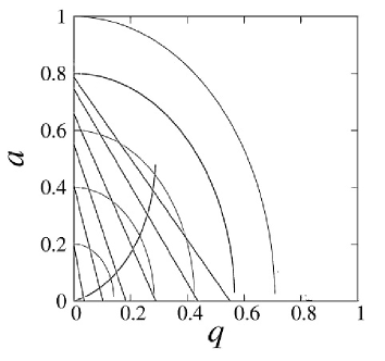
(b)

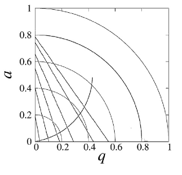
(c)

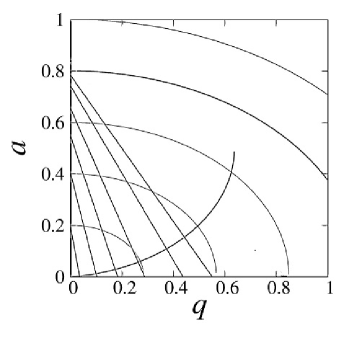
Figure 6: The solid thick curve shows the trajectory of the optimum strategy to reduce the epidemic peak for $\gamma=0.06$. Straight lines are constant $y^{*}$ lines: $y^{*}=0.5,0.4,0.3,0.2,0.1,0.05$ from left to right, and oval curves represent constant cost curves: $C=0.04,0.16,0.36,0.64,1$ from left to right. (a) $k=2$, (b) $k=1$ and (c) $k=0.5$.

4.3 Optimum measure to stamp out the epidemic

In this subsection, I discuss an optimum measure to stamp out the epidemic at the beginning of the outbreak. The growth rate of the number of infected at large is given by Eq. (22) in the early stage of the outbreak, and I set

$${\cal M}(a,q)=(1-a)\beta_{0}-q-\gamma.$$ (30)

The aim of a measure is to bring the state from the region ${\cal M}(a,q)>0$ at $(a=0,q=0)$ to some region ${\cal M}(a,q)<0$.

It is straightforward to find that the optimum trajectory $(a^{*},q^{*})$ satisfies

$$a^{*}=k\frac{q^{*}}{\beta_{0}}.$$ (31)

Figure 7 shows the optimum trajectory on the $(a,q)$ plane: (a) $k=2$, (b) $k=1$ and (c) $k=0.5$.

(a)

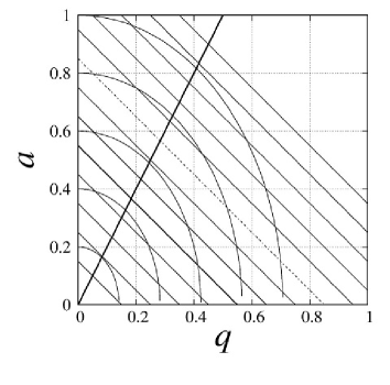
(b)

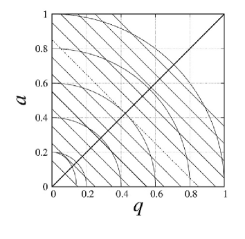
(c)

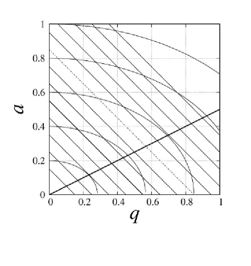
Figure 7: The increasing thick straight line is the trajectory of the optimum strategy to stamp out the epidemic for $\gamma=0.06$. Decreasing straight lines shows the constant growth rate lines from 0.7 (the lowest line)to -0.4 (the highest line), and the dashed line shows $\lambda=0$. Oval curves represent constant cost curves: $C=0.04,0.16,0.36,0.64,1$ from left to right. (a) $k=2$, (b) $k=1$ and (c) $k=0.5$.

5 Discussion

In this paper, I presented exact properties of the SIQR model relevant to COVID-19 in the entire time span and in the early stage of the outbreak. In particular, I investigated dependence of the outbreak on parameters, transmission coefficient and quarantine rate, which can be controlled by measures. It is important to note that the peak of the number of quarantined patients $w(t)$ appears about 10 days later than the time that the number of infected $y(t)$ becomes maximum, for the choice of parameters used in Fig. 4. Within this model, the number of infected at large $y(t)$ can be estimated from the daily confirmed new cases $\Delta w(t)$, once the quarantine rate $q$ is obtained from the infection trajectory. I also discussed a theoretical framework for optimizing measures to control the outbreak on the basis of the expected utility theory, when the social cost is given by a function of the social distancing policy and the quarantine measure. The optimum strategy depends on the aim; reducing the epidemic peak or accelerating the stamping out the outbreak. It should be emphasized that a simple lockdown ($a=1$) is not the optimum strategy.

Given the cost function and the aim of policy in each country, it will be possible to formulate the optimum policy specific to the country for controlling the outbreak on the basis of the present theoretical framework.

The SIQR model does not consider any memory effects of the epidemic like the incubation period and the infectious period functions. It is an important future problem to include memory effects of $\beta$ and $q$ in the SIQR model.

References

-
[1]
Coronavirus Resource Center, Johns Hopkins University
https://coronavirus.jhu.edu/ -
[2]
N. M. Ferguson, D. Laydon, G. Nedjati-Gilani et al. ”Impact of non-pharmaceutical
interventions (NPIs) to reduce COVID-19 mortality and healthcare demand”.
Imperial College London (16-03-2020).
doi:https://doi.org/10.25561/77482. - [3] W. O. Kermack and A. G. McKendrick, Proc. Roy. Soc. A 115, 700-721 (1927).
- [4] R. M. Anderson and R. M. May, Science 215, 1053-1060 (1982).
- [5] H. Hethcote, M. Zhien and L. Shengbing, Math. Biosciences 180, 141-160 (2002).
- [6] W. Jumpen, B. Wiwatanapataphee, Y.H. Wu and I. M. Tang, Int. J. Pure and Appl. Math. 52, 247-265 (2009).
- [7] M. G. Pedersen and M. Meneghini, https://doi.org/10.13140/RG.2.2.11753.85600
- [8] A. Tiwari, https://doi.org/10.1101/2020.04.12.20062794
- [9] A. Tiwari, https://doi.org/10.1101/2020.06.08.20125658
- [10] L. Sedov. A. Krasnochub and V. Polishchuk, https://doi.org/10.1101/2020.04.15.20067025
- [11] T. Odagaki, https://10.1101/2020.06.02.20117341
-
[12]
J. S. Coleman, “Foundations of Social Theory”, (Harvard University Press,
Cambridge, 1990).
- [13] T. Harko, F. S. N. Francisco and M. K. Mak, Appl. Math. Comp. 236, 184-194 (2014).
- [14] X. Yan, Y. Zou and J. Li, World J. Model. Simul. 3,202-218 (2007).