pnassupportinginfo

Additional information about the X-ray imaging diagnostic

Framing camera response

The responses of the various components of the X-ray framing camera, along with the combined temperature response, is shown in Figure 1.

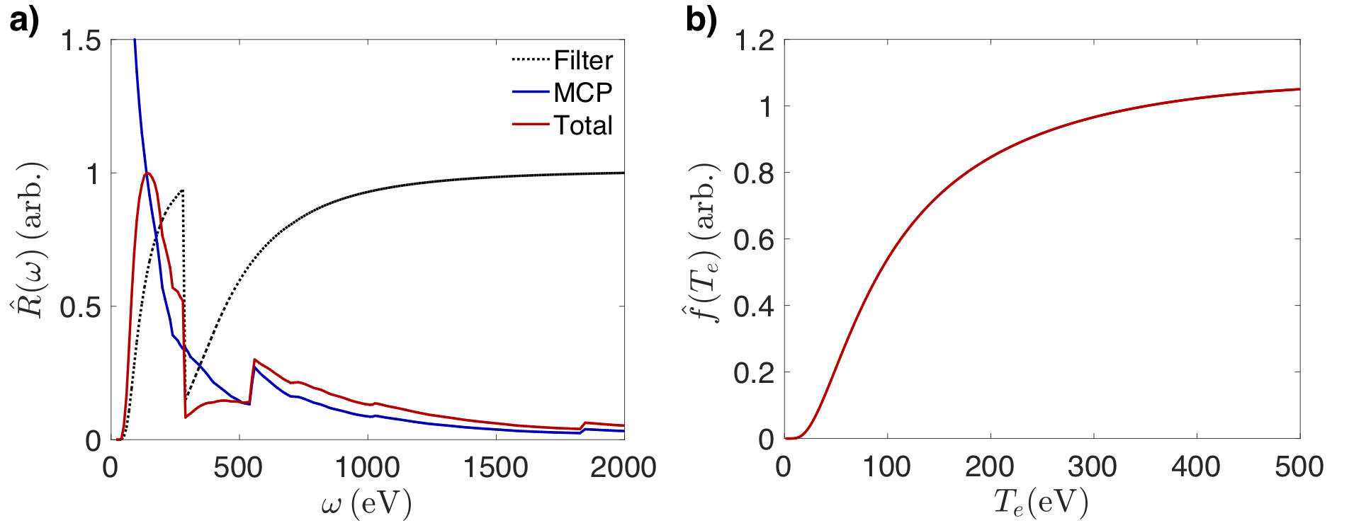
Figure 1: Response of the X-ray framing camera. a) Response functions $\hat{R}(\omega)$ associated with the X-ray framing camera filter alone (black, dotted), the microchannel plate alone (blue), and the combined response (red). The total response and the filter response are normalized to their respective maximum values; the MCP response is normalized to its value at the frequency at which the total response is maximized. b) Relative temperature dependence of the measured optical intensity on the CCD camera. The temperature is normalized to its value at $T_{e}=350\,\mathrm{eV}$.

Calculation of mean X-ray emission profiles

The mean emission profiles shown in Figure 2 of the main text are calculated via direct application to the images of a 57 $\times$ 57 pixel mean filter. With a pixel size of $9\,\mu\mathrm{m}$, this corresponds to assuming that the mean emission profile varies smoothly on scales $\gtrsim 500\,\mu\mathrm{m}$; the largest relative fluctuations inside the interaction region have typical size $L\lesssim 200-400\,\mu\mathrm{m}$, providing a modest scale separation. However, applying only a mean filter to the images is inadequate for determining reasonable mean emission profiles; the presence of shocks on either side of the interaction-region plasma implies that the global emission profile would in reality have sharp boundaries (on scales $\lesssim 500\,\mu\mathrm{m}$), a feature not adequately picked up by a linear filter. This phenomenon is evident in Figure 3 of the main text, where the X-ray emission is observed to drop rapidly over $\sim 10-20$ pixels ($\sim 100-200\,\mu$m). To account for this, a two-dimensional Gaussian window function on the scale of the boundary is combined with the mean emission profile to prevent the boundary region from distorting the calculated relative X-ray intensity map (similar techniques are also applied in spectral analysis of data with gaps (1)).

Semi-deterministic feature of relative X-ray intensity maps

For a few of the relative intensity maps that we extracted – for example, that shown in Figure 4b of the main text – we note that positively signed intensity fluctuations seem to be more concentrated near the equatorial plane of the interaction region, whereas negatively signed intensity fluctuations are more concentrated on the sides. In the raw X-ray images from which these particular relative intensity maps were derived, a sudden drop in emission between the central part of the interaction region is discernible by eye, suggesting that this feature is physical, rather than a numerical artifact of the algorithm separating the mean emission profile from the relative-intensity profile. We believe this feature is due to the interaction-region plasma not in fact being a flat disk, but instead being ‘buckled’. It is therefore possible that the sharp drop in emission in the outer regions of the interaction region is due to a sudden decrease in the effective path length over which the plasma emits. Such an effect would not be captured by the algorithm that was used to determine the mean density profile. This interpretation is supported by the FLASH simulations of the experiment: the simulated interaction-region plasma is indeed buckled, and the aforementioned feature is evident in simulated X-ray images of the plasma (see below). The presence of this feature in some images but not others suggests that this distortion of the interaction-region shape may depend on the particular stochastic motions that emerge after the region forms. We emphasize that we find that all of our X-ray images at $t>31$ ns lead to a similar density spectrum (including those in which the concentration of positively signed intensity fluctuations near the equatorial plane of the interaction region is much less prominent), and thus believe that our conclusions concerning the properties of fluctuations are not significantly affected by the presence of this feature.

Additional information on the Thomson-scattering diagnostic

Raw spatially resolved Thomson-scattering spectra

Figure 2 shows the raw data from the spatially resolved Thomson-scattering diagnostic at times close to the interaction-region formation (Figures 2a to 2d are the IAW features and Figures 2e to 2h the EPW features).

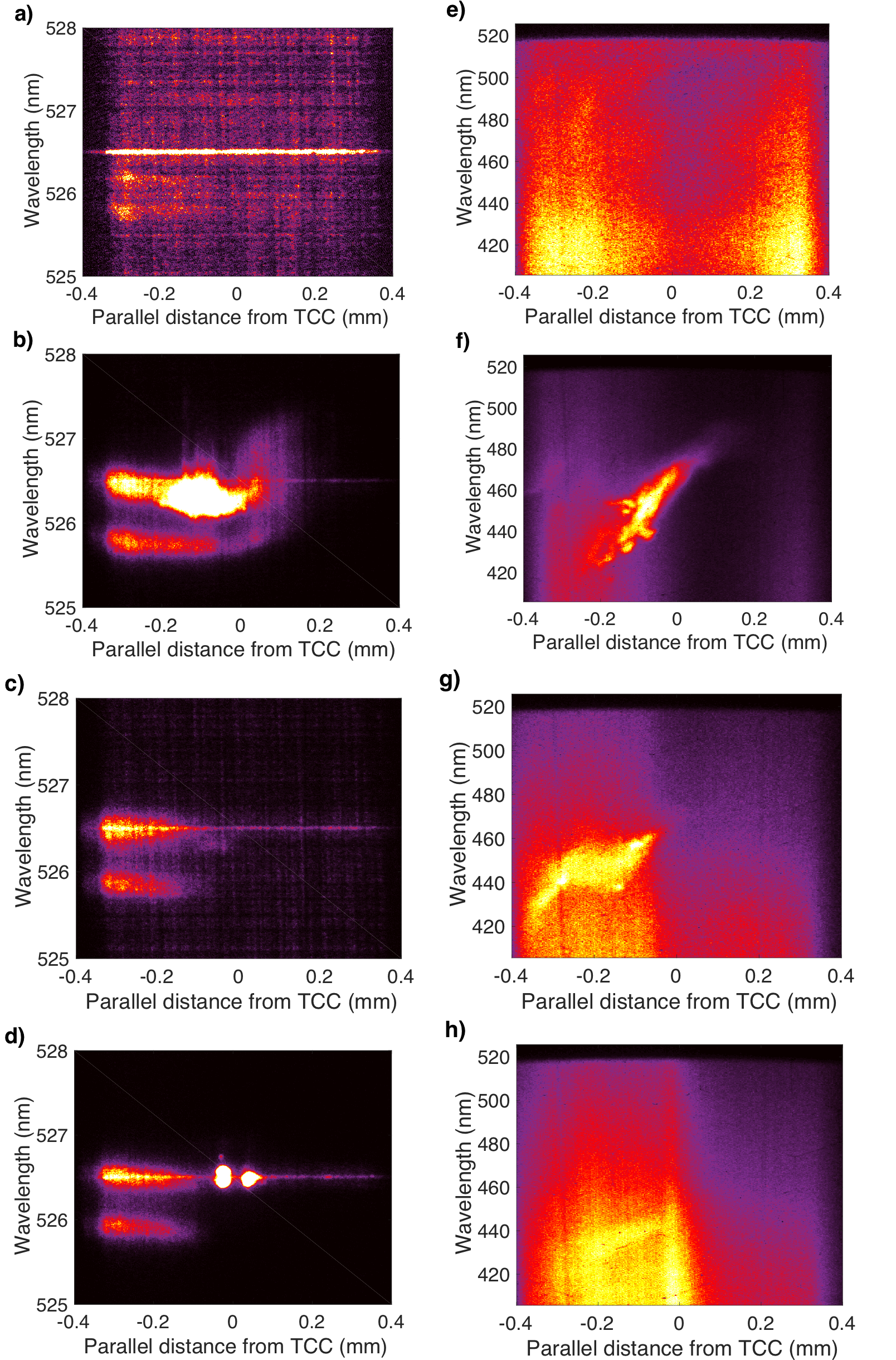
Figure 2: Experimental Thomson-scattering spectra at the time of the interaction-region formation. The low-frequency spectra (IAW features) are shown in the left column (a-d) and the high-frequency spectra (EPW features) in the right column (e-h). The scattering volume is orientated at a 63^∘ angle to the direction parallel to the line of centers; for convenience of reference to the X-ray images, we report distances projected onto the line of centers. The timings of the images are as follows: a), e), 24.0 ns; e), f) 25.5 ns; c), g) 27.0 ns; d), h) 28.5 ns.

The Thomson-scattering data used to extract the effective ion temperature and flow velocities at late times is shown in Figure 3.

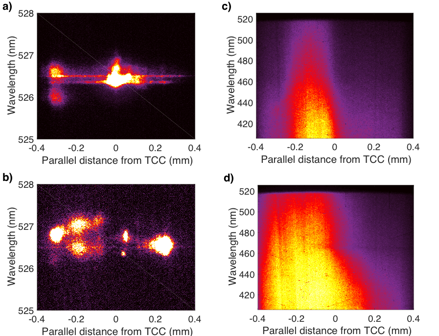
Figure 3: Experimental Thomson-scattering spectra at later times. The low-frequency spectra (IAW features) are shown in the left column (a-b) and the high-frequency spectra (EPW features) in the right column (c-d). The timings of the images are as follows: a), c), 30.0 ns; b), d) 37.5 ns.

Additional information on spectral fitting procedure

We illustrate the spectral fitting procedure used to extract bulk plasma parameters with two examples. Figure 4a shows the IAW feature at 27.0 ns after the laser pulse.

Figure 4: Fitting the IAW feature. a) IAW spectrum from 27.0 ns after drive-beam pulse initiation. In (b-d), the experimental 1D spectrum (in red) is calculated by averaging the full spectrum horizontally over the region denoted by the translucent rectangle. b) Experimental spectrum: the best-fit spectrum ($T_{e}=470\,\mathrm{eV}$, $T_{i,\mathrm{eff}}=620\,\mathrm{eV}$, $\bar{u}_{\rm in}=230\,\mathrm{km}\;\mathrm{s}^{-1}$, $n_{e}=1.2\times 10^{20}\,\mathrm{cm}^{-3}$) in solid blue, and the fits parametrized by $T_{e}$ sensitivity bounds (-30% dashed, +30% dotted). All fits are convolved with the (experimentally measured) instrument function, which has a characteristic width of 0.025 nm. The sharp peak seen at the probe-beam wavelength ($526.5\,\mathrm{nm}$) is the so-called ‘stray-light’ feature, and is not part of the plasma’s Thomson-scattering spectrum; it is disregarded for the purposes of fitting. c) Same as b) but the fits parametrized by $\bar{u}_{\rm in}$ sensitivity bounds are plotted. d) Same as b) but the fits parametrized by $T_{i,\mathrm{eff}}$ sensitivity bounds are plotted.

To fit the experimental spectrum at a given position, we first average it over a 100 $\mu$m interval centered at that position. We then calculate a fit using Eq. [13] of the main text, substituting the dispersion relation $\omega=\omega(k)$ for a light wave propagating through plasma, and adjusting $T_{e}$, $T_{i}$, $\bar{u}_{\|}$ and $\Delta u$. In the chosen geometry of the diagnostic, the bulk velocity parallel to $\hat{\boldsymbol{k}}$ is equal to the inflow velocity $\bar{u}_{\rm in}$ parallel to the target’s line of centers, i.e., $\bar{u}_{\|}=\bar{u}_{\rm in}$. We do not use an absolute calibration of the spectrum for the fit, but instead normalize the height of the theoretical spectrum to the lower-wavelength experimental peak (the higher-wavelength experimental peak is typically distorted by a stray-light feature). Once a best fit is obtained, we then adjust each parameter individually to assess the sensitivity of the fit. Figures 4b and 4c demonstrate this process for the electron temperature $T_{e}$ and velocity $\Delta u$, respectively: we find sensitivities of $\pm 30\%$ for $T_{e}$ and $\pm 15\%$ for $\bar{u}_{\rm in}$. Fitting $T_{i}$ and $\Delta u$ is more subtle because both quantities have a similar effect on the shape of the spectrum (they affect the width of the spectral peaks). We therefore instead choose to fit an effective ion temperature, $T_{i,\mathrm{eff}}$ including both thermal broadening and one due to small-scale stochastic motion. The sensitivity of the fit for $T_{i,\mathrm{eff}}$ is found to be $\pm 40\%$. To determine independently $T_{i}$ and $\Delta u$, we then use the fact that motions are subsonic and thus estimate $\Delta u\approx c_{\mathrm{s}}\Delta n_{e}/\bar{n}_{e}$, where $c_{\mathrm{s}}$ is the sound speed; this leaves $T_{i}$ as the only free parameter determining $T_{i,\mathrm{eff}}$ in the fits. It is in general true that the sensitivity of a fit can be underestimated systematically using our chosen methodology – that is, fixing all physical parameters for the fits save one, and then varying the chosen parameter to determine the sensitivity. However, on account of couplings between parameters, such considerations do not apply to the IAW fits. This is because the parameters $\Delta u$, $T_{e}$, and $T_{i,\mathrm{eff}}$ each only influence one characteristic of the fit: the average peak position, peak separation and peak width, respectively.

Figure 5a shows the EPW feature for the same experimental shot.

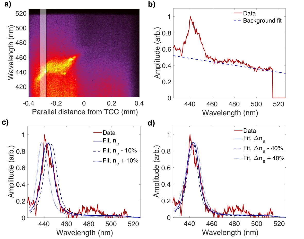
Figure 5: Fitting the EPW feature. a) EPW spectrum from 27.0 ns after drive-beam pulse initiation. In (b-d), the experimental 1D spectrum (in red) is calculated by averaging the full spectrum horizontally over the region denoted by the translucent rectangle. b) The linear background fit to the raw experimental spectrum. c) Background-subtracted experimental spectrum: the best-fit spectrum ($T_{e}=470\,\mathrm{eV}$, $T_{i,\mathrm{eff}}=620\,\mathrm{eV}$, $\bar{u}_{\rm in}=230\,\mathrm{km}\;\mathrm{s}^{-1}$, $\bar{n}_{e}=1.2\times 10^{20}\,\mathrm{cm}^{-3}$, $\Delta n_{e}=0.35\times 10^{20}\,\mathrm{cm}^{-3}$) in solid blue, and the fits parametrized by $\bar{n}_{e}$ sensitivity bounds (-10% dashed, +10% dotted). All fits are convolved with the (experimentally measured) instrument function, which has a characteristic width of 0.025 nm. d) Same as b) but fits parametrized by $\Delta n_{e}$ sensitivity bounds are plotted.

We again determine the experimental EPW spectrum at a given position by averaging over a $100\,\mu\mathrm{m}$ interval. Before attempting to fit the EPW spectrum, we must first correct for the CCD/grating response, as well as subtract the background signal. The latter is more significant for the EPW spectrum than for the IAW spectrum – on account of the former’s smaller magnitude – and is most likely to be associated with radiative emission from the plasma. We find that the background signal for our data is well characterized by a linear fit (see Figure 5b). We then fit the experimental spectrum by varying $\bar{n}_{e}$ and $\Delta n_{e}$, before determining the sensitivity of the fits to variations in these quantities: we find $\pm 10\%$ for $\bar{n}_{e}$ (Figure 5c) and $\pm 40\%$ for $\Delta n_{e}$ (Figure 5d). As with the IAW fits, $\bar{n}_{e}$ and $\Delta n_{e}$ affect different characteristics of the EPW fit, so our methodology for assessing the fit sensitivity is appropriate. However, we note that the peak position of the EPW feature can be weakly sensitive to the assumed electron temperature as well as to $\bar{n}_{e}$; since the electron temperature is held constant when fitting the EPW feature, using the value determined from the IAW feature, the quoted $\pm 10\%$ sensitivity for $\bar{n}_{e}$ could in practice be a slight underestimate. Nonetheless, we do not believe it worthwhile carrying out a multivariate assessment of the fit’s sensitivity, because the ratio of the change in peak position arising from an order-unity change in the electron temperature to the change in peak position due to an order-unity change in the mean electron density is anticipated theoretically to be $\mathcal{O}(\alpha^{-2})\ll 1$ (we remind the reader that $\alpha\equiv 1/k\lambda_{\rm{D}}$). Since the uncertainty in $T_{e}$ from the IAW fit is $\pm 30\%$, we conclude that corrections to the sensitivity in $\bar{n}_{e}$ due to the uncertainty in $T_{e}$ will be no more than a few percent.

Perturbative heating effects of Thomson-scattering diagnostic

Whilst analyzing the results of our experiment, we discovered that our Thomson-scattering diagnostic was not always non-invasive, particularly at late times. Indirect evidence of this observation is most easily obtained from our X-ray imaging diagnostic. As mentioned in Materials and Methods, for a given experimental shot, two X-ray imaging times were recorded; the earlier time was always chosen to fall before the application of the other diagnostics, and the later time after. This allowed us to assess whether invasive effects – in particular, additional heating – associated with our experimental diagnostics were significant.

Two sample X-ray images arising from one particular experimental shot timed according to these arrangements are shown in Figure 6.

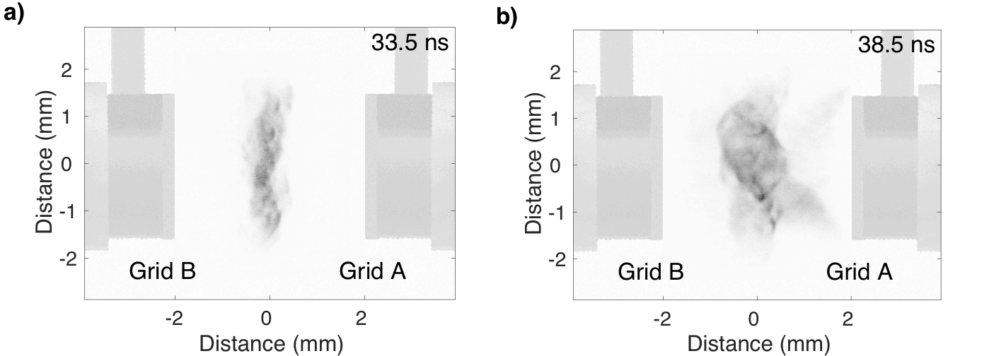
Figure 6: Imaging self-emitted X-rays for each experimental shot. Characteristic output images from X-ray framing camera diagnostic in a sample experimental shot. In both images, the color map is linear and adjusted so that the maximum displayed pixel value is 1,050 (corresponding to the maximum pixel count of all our experimental images). The images shown have been cropped and are both 870 $\times$ 641 pixels. To aid interpretation of the images, an outline of the target has been superimposed onto both images. The respective designs of grid A and B are shown in Figure 1 of the main text, bottom right. a) The X-ray image recorded with the first MCP strip 33.5 ns after the drive-beams are initiated. On this experimental shot, the Thomson-scattering probe beam was initiated 1 ns after the first MCP strip was gated and the proton backlighter capsule irradiated 2.5 ns later; thus, the self-emitted X-rays detected in the image are purely due to the interaction-region plasma’s dynamics. b) The X-ray image recorded with the second MCP strip 38.5 ns after the drive beams are initiated. This image was recorded after both the Thomson-scattering probe beam and the proton backlighter were used.

Comparing Figure 6a and 6b, we see that, in addition to the dynamical evolution of the interaction region, increased emission is observed in the later image from plasma between grid A and the central interaction-region plasma. This effect is most likely due to the aforementioned heating; the diagonal feature corresponds to the projected trajectory of the Thomson-scattering beam and only the plasma between grid A and the target center is visible to the proton backlighter capsule. We henceforth refer to the earlier-time images as ‘unperturbed’ self-emission X-ray images and the later ones as ‘perturbed’ images. All X-ray images presented in the main text are unperturbed images. For reference, the perturbed images corresponding to the unperturbed images shown in Figure 3 of the main text are presented in Figure 7.

Figure 7: The interaction-region plasma’s evolution in the presence of perturbative diagnostic heating. Perturbed self-emission X-ray images of the interaction-region plasma. The parameters of each column are identical to those of Figure 2 in the main text. We note that the CCD camera used to record this sequence of images was damaged in a small localized region slightly below the center of each image; we therefore chose our window functions so that this region was excluded from subsequent analysis.

From our measurements of bulk plasma parameters, the claim that the Thomson-scattering probe beam heats the plasma can be justified as follows. The fraction $f_{a}$ of the probe beam’s energy absorbed by the plasma can be estimated as $f_{a}\approx 1-\exp{(-\kappa_{a}l_{\mathrm{beam}})}$, where $\kappa_{a}$ is the the absorption coefficient of the beam in the plasma and $l_{\mathrm{beam}}$ the path length of the beam through the interaction-region plasma (2). The dominant absorption process affecting the beam is inverse bremsstrahlung, so

$$\kappa_{a} = 3.6\left[\frac{Z_{\mathrm{eff}}}{5.3}\right]\left[\frac{\log\Lambda}{7}\right]\left[\frac{n_{e}(\mathrm{cm}^{-3})}{1.5\times 10^{20}\,\mathrm{cm}^{-3}}\right]^{2}\left[\frac{T_{e}(\mathrm{eV})}{330\,\mathrm{eV}}\right]^{-3/2}\left[\frac{\omega_{0}(\mathrm{s}^{-1})}{3.6\times 10^{15}\,\mathrm{s}^{-1}}\right]^{-2}\left[\frac{\epsilon_{\rm D}}{0.97}\right]^{-1/2}\,\mathrm{cm}^{-1},$$ (1)

where $\epsilon_{\rm D}\equiv 1-\omega_{\mathrm{p}e}^{2}/\omega_{0}^{2}$ is the dielectric permittivity of the plasma. Estimating $l_{\mathrm{beam}}\approx 0.13\,\mathrm{cm}$ from the X-ray measurements of the interaction-region width at 38.5 ns, we conclude that $\kappa_{a}l_{\mathrm{beam}}\approx 0.45$ and thus $f_{a}\approx 0.36$. Therefore, the total energy deposited in the Thomson-scattering volume (neglecting conduction) is $E_{\mathrm{heat}}\approx 1.1\times 10^{8}\,\mathrm{erg}$. Noting that the internal-energy density of the plasma is $\varepsilon_{\rm th}\approx 3n_{e}T_{e}\left(1+\langle Z\rangle^{-1}\right)/2$ (assuming $T_{i}\approx T_{e}$), it follows that the total thermal energy $E_{\mathrm{th}}$ present in the Thomson-scattering volume is

$$E_{\mathrm{th}}=1.1\times 10^{8}\left[\frac{\langle Z\rangle+1}{4.5}\right]\left[\frac{n_{e}(\mathrm{cm}^{-3})}{1.5\times 10^{20}\,\mathrm{cm}^{-3}}\right]\left[\frac{T_{e}(\mathrm{eV})}{330\,\mathrm{eV}}\right]\left[\frac{\mathcal{V}_{\rm T}(\mathrm{cm}^{3})}{7.5\times 10^{-4}\,\mathrm{cm}^{3}}\right]\,\mathrm{erg}\,,$$ (2)

where $\mathcal{V}_{\rm T}$ is the volume of the Thomson-scattering collection region. We conclude that at the given density, $E_{\mathrm{heat}}\gtrsim E_{\mathrm{th}}$ for electron temperatures $T_{e}\lesssim 330\,\mathrm{eV}$. It follows that the electron temperature at later times could be significantly lower than the value measured by the Thomson-scattering beam in the absence of the probe-beam heating.

We now consider the effects of this diagnostic heating on our results. Figures 8a and 8b compare the X-ray self-emission from the plasma $\sim 3\,\mathrm{ns}$ after the jet collision (which is at $\sim 26\,\mathrm{ns}$) in the absence and presence, respectively, of probe-beam heating; the equivalent comparison $\sim 12.5\,\mathrm{ns}$ after the jet collision is given by Figures 8c and 8d.

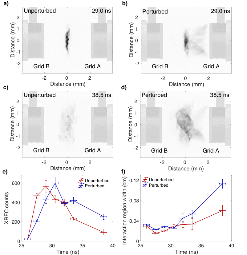
Figure 8: Perturbed versus unperturbed self-emission X-ray images. a) Self-emission X-ray image at 29.0 ns after the initiation of the drive-beam pulse, in the absence of perturbative diagnostics. The color map of the image is the same as Figure 6. b) Same as a), except in the presence of perturbative diagnostics. c) Unperturbed X-ray image at 38.5 ns. d) Perturbed X-ray image at 38.5 ns. e) Evolution of mean maximum value of one-dimensional mean emission profiles over time for unperturbed (red) and perturbed (blue) X-ray images. The error in each measurement is the error arising from the three distinct lineouts calculated from different perpendicular positions in the interaction-region plasma – see Figure 4a). f) Mean-interaction width over time for the unperturbed and perturbed X-ray images. The width and errors are calculated in the same manner as described in the caption of Figure 4 of the main text.

Qualitatively, we note that emission from the interaction-region plasma itself in the former case is not obviously different in the perturbed and unperturbed images: the absolute value of the emission is similar, as is the morphology of the region. However, at later times, emission from the perturbed X-ray images is noticeably higher. More quantitatively, we use the maximum pixel values of the one-dimensional mean emission profiles used to calculate the interaction region width (cf. Figure 4 of the main text) to compare the relative emission levels associated with the unperturbed and perturbed cases, respectively (Figure 8e). Somewhat unexpectedly, we find that, immediately after the interaction-region formation, the emission from the unperturbed cases is greater. This trend is most likely explained by thermal expansion of the interaction-region plasma induced by the additional diagnostic heating: although higher temperatures would result in slightly increased emission, this trend would be counteracted by lower mean densities in the expanded interaction region, particularly since the measured X-ray intensity is much more strongly dependent on density than on temperature for $T_{e}\sim 300-500\,\mathrm{eV}$. This argument is given some weight by the observation that the measured interaction-region width in the perturbed images is slightly larger (Figure 8f) immediately after collision. At later times, Figure 8e illustrates the (expected) trend of significantly reduced X-ray intensity in the unperturbed images compared to the perturbed ones. The most likely explanation of this observation is a lower temperature of the interaction-region plasma in the unperturbed case ($T_{e}\sim 50-100$ eV).

We can, in fact, use the observed changes in self-emitted X-ray intensity (combined with the Thomson-scattering measurements) to derive a more precise estimate of the amount of heating. We recall that the intensity $I$ recorded by the CCD camera depends on temperature: $I\propto\int\mathrm{d}s\,n_{e}^{2}\hat{f}(T_{e})$, where $\hat{f}(T_{e})$ is defined by Eq. [2] of the main text and plotted in Figure 1b. Thus, if the electron number density of the interaction-region plasma is known at two given times, any difference in total intensity evident in an X-ray image can be attributed to distinct temperatures. Applying this logic to unperturbed and perturbed X-ray images recorded at the same point in time (in different experimental shots) and assuming that at later times probe-beam heating has a negligible effect on plasma density, we can use the differences in intensity calculated in Figure 8f to estimate the unperturbed electron temperature $(T_{e})_{\mathrm{up}}$. Namely, it follows that $(T_{e})_{\mathrm{up}}\approx(T_{e})_{\mathrm{p}}\hat{f}^{-1}\left({I_{\mathrm{up}}}/{I_{\mathrm{p}}}\right)\approx 75\,\mathrm{eV}$, where $(T_{e})_{\mathrm{p}}$ is the perturbed electron temperature, $I_{\mathrm{p}}$ the mean X-ray intensity in the unperturbed image, and $I_{\mathrm{up}}$ the mean X-ray intensity in the perturbed image. This inferred bound is significantly below the temperature measured by the Thomson-scattering diagnostic.

We confirm the importance of the Thomson-scattering probe beam heating using the FLASH simulations – see ‘Overview of FLASH simulations of experiment’.

Additional information on the proton-imaging diagnostic

Parameterized one-dimensional model for the path-integrated magnetic field arising from the double-cocoon configuration

In the main text, we employ a double-cocoon configuration to describe the magnetic field at the time of interaction-region formation; we further claim that if the parallel scale of the cocoons is much smaller than their perpendicular scale, then the path-integrated field experienced by imaging protons is quasi-one-dimensional, and is oriented in the (unique) direction that is perpendicular both to the imaging protons’ direction and the axis of symmetry of the cocoons. We validate this claim here.

The double-cocoon configuration is constructed from the simple model of a single cocoon provided by (3), in which the magnetic field $\boldsymbol{B}$ is given by

$$\boldsymbol{B}=\sqrt{2}B_{\rm max}\frac{r}{a}e^{\frac{a^{2}-2r^{2}}{2a^{2}}-\frac{z^{2}}{b^{2}}}\boldsymbol{e}_{\phi}\,,$$ (3)

where $(r,\phi,z)$ is a cylindrical coordinate system with symmetry axis $z$, $B_{\rm max}$ is the maximum magnetic-field strength, $a$ the characteristic perpendicular size of the cocoon, $b$ the characteristic parallel size of the cocoon, and $\boldsymbol{e}_{\phi}$ the azimuthal unit vector. It is shown in (3) that the path-integrated magnetic field associated with such a structure when viewed at an angle $\theta$ with respect to the $z$ axis is

$$\int\mathrm{d}s\,B_{1} = \frac{B_{\rm max}a^{2}b\sqrt{2\pi}\cos\theta}{d^{2}}\frac{u_{2}}{d}e^{\frac{1-2u_{1}^{2}}{2a^{2}}-\frac{u_{2}^{2}}{d^{2}}}\,,$$ (4)

$$\int\mathrm{d}s\,B_{2} = -\frac{B_{\rm max}ab\sqrt{2\pi}\cos\theta}{d}\frac{u_{1}}{a}e^{\frac{1-2u_{1}^{2}}{2a^{2}}-\frac{u_{2}^{2}}{d^{2}}}\,,$$ (5)

where

$$d\equiv\sqrt{a^{2}\cos^{2}\theta+b^{2}\sin^{2}\theta}\,.$$ (6)

Here the two-dimensional Cartesian coordinate system $(u_{1},u_{2})$ is chosen to be perpendicular to the viewing direction, with basis vectors satisfying $\hat{\boldsymbol{e}}_{1}\cdot\hat{\boldsymbol{z}}=0$, $\hat{\boldsymbol{e}}_{2}\cdot\hat{\boldsymbol{z}}\neq 0$, $B_{1}\equiv\boldsymbol{B}\cdot\hat{\boldsymbol{e}}_{1}$ and $B_{2}\equiv\boldsymbol{B}\cdot\hat{\boldsymbol{e}}_{2}$. If we assume that the perpendicular extent of the cocoon structures is much greater than the parallel extent, viz., $a\gg b$, it follows that for angles $\theta$ such that $\pi/2-\theta\gg b/a$, $d\approx a\cos\theta$. For our experiment, $\theta\approx 55^{\circ}$, so $d\approx a/\sqrt{3}$. Under these assumptions, Eqs. [4] and [5] become

$$\int\mathrm{d}s\,B_{1} \approx 3B_{\rm max}b\sqrt{2\pi}\frac{u_{2}}{a}e^{\frac{1-2u_{1}^{2}}{2a^{2}}-3\frac{u_{2}^{2}}{a^{2}}}\,,$$ (7)

$$\int\mathrm{d}s\,B_{2} \approx -B_{\rm max}b\sqrt{2\pi}\frac{u_{1}}{a}e^{\frac{1-2u_{1}^{2}}{2a^{2}}-3\frac{u_{2}^{2}}{a^{2}}}\,.$$ (8)

We conclude that in such a model, the path-integrated field is indeed elongated in the $u_{1}$ direction (which by definition is precisely the direction perpendicular to the projected line of centers), and, for $u_{1}\lesssim u_{2}$, the path-integrated perpendicular magnetic field is also predominantly in the $u_{1}$ direction.

For the double-cocoon configuration, we therefore obtain

$$\int\mathrm{d}s\,\boldsymbol{B} \approx 3\sqrt{2\pi}\mathrm{e}^{\frac{u_{1}^{2}-2a^{2}}{2a^{2}}}\Bigg{[}bB_{\rm max}^{+}\frac{u_{2}+\tilde{\ell}_{c}}{a}\mathrm{e}^{-\frac{3(u_{2}+\tilde{\ell}_{c})^{2}}{a^{2}}}+bB_{\rm max}^{-}\frac{u_{2}-\tilde{\ell}_{c}}{a}\mathrm{e}^{-\frac{3(u_{2}-\tilde{\ell}_{c})^{2}}{a^{2}}}\Bigg{]}\hat{\boldsymbol{e}}_{1}\,,$$ (9)

where $\tilde{\ell}_{c}\approx\sqrt{2}\ell_{c}/\sqrt{3}$. Eq. [9] is the quasi-one-dimensional model for the path-integrated magnetic field employed in the main text.

Validating the double-cocoon configuration

As a further check of the accuracy of our double-cocoon model, we calculate the predicted one-dimensional profile of proton flux associated with this model, and compare the result to a one-dimensional lineout calculated directly from the relevant proton image in the same region as was used to determine the experimental path-integrated-field profile (see Figures 9a and 9b). We find that the predicted profile is a close match to the experimental one.

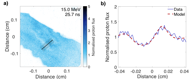
Figure 9: Validating the double-cocoon model for the magnetic field at the time of interaction-region formation. a) The 15.0 MeV proton image from which Figure 6a of the main text is calculated, portrayed with the translucent rectangular region. b) One-dimensional lineout of the normalized proton flux (blue, solid line) calculated by averaging translucent rectangular region denoted in a) across its width, along with one-dimensional prediction from model [4] of the main text using the optimized parameters given in the caption of Figure 6.

Heuristic estimate of magnetic-field strength at the time of interaction-region formation

An alternative, simple way of estimating the average strength of the magnetic field in the interaction region is to calculate the mean value of the path-integrated perpendicular magnetic field and divide it by the path length $l_{p}$ of the protons through the interaction region. We do this for our data by first evaluating $\langle|\int\mathrm{d}^{2}\boldsymbol{x}\,\boldsymbol{B}_{\perp}^{\prime}|\rangle$ in three square regions (see Figure 7a of the main text and the caption for their precise dimensions), and determining the mean value (and errors) across the three regions. We then determine $l_{p}$ as described in the main text. Finally, we estimate $\langle B\rangle$ via $\langle B\rangle\approx\langle|\int\mathrm{d}^{2}\boldsymbol{x}\,\boldsymbol{B}_{\perp}^{\prime}|\rangle/l_{p}$. We obtain $\langle B\rangle\approx 6\,\mathrm{kG}$, in agreement with the parameterized double-cocoon configuration.

However, such an estimate implicitly makes a number of assumptions about the nature of the underlying structure of the (non-stochastic) magnetic field. First, components of the magnetic field parallel to the path of the proton-imaging beam are assumed to be negligible compared to perpendicular components. Secondly, the estimate presupposes that the path-integrated field does not change sign along the path. We can, however, assess the validity of these two assumptions using our parameterized double-cocoon model of the magnetic field at the time of interaction-region formation. Inside the rectangular region to which we have applied our model, the magnetic field is predominantly in the $x$ direction, so the component parallel to the protons’ path is indeed small. Due to the $55^{\circ}$ angle of imaging, the $B_{x}$ components of the opposing cocoon structures add constructively rather than destructively at all positions. Thus, we conclude that the stated assumptions are reasonable at least for the strongest path-integrated structure.

Testing statistical assumptions about stochastic magnetic fields in our experiment

In the main text, we claim that the stochastic magnetic fields produced after the interaction-region formation can be assumed to be statistically homogeneous and isotropic within the plasma. Here we test that assumption. Figure 10a shows the magnetic-energy spectra calculated using Eq. [7] of the main text for the three chosen regions in the case of the path-integrated fields calculated at 27.2 ns since the initiation of the drive beams.

Figure 10: Validating assumed statistical symmetries of stochastic magnetic fields subsequent to interaction-region formation. a) Test of statistical homogeneity of the stochastic magnetic field. The magnetic-energy spectra associated with the left, middle and right square regions shown in Figure 7 of the main text (which are calculated using Eq. [7]) are plotted, along with the nominal resolution of the proton-imaging diagnostic and the grid scale. The slope $k^{-3}$ is plotted for reference, but does not have physical significance. b) Test of statistical isotropy of the stochastic magnetic field. For each square region, the magnetic-energy spectrum associated with wavenumbers predominantly parallel to the line of centers is calculated by determining the spectral slope from magnetic-field Fourier components with $k_{\|}>k_{\perp}$, and vice versa for the magnetic-energy spectrum associated with predominantly perpendicular wavenumbers. Mean parallel and perpendicular spectra are subsequently obtained by averaging the results from each region (the errors are determined similarly).

Except at the largest scales, we find that the three spectra match closely, supporting the homogeneity assumption. The isotropy assumption is tested in Figure 10b. Given the symmetry of our experiment, any anisotropy would manifest itself with respect to the line of centers. So, in each box, we calculate the magnetic-energy spectra both for wavenumbers predominantly parallel to the projected line of centers, and for those predominately perpendicular to it. The results are then combined to obtain averaged parallel and perpendicular spectra. We find that the two spectra are the same within the uncertainty of the measurement.

Plasma characterization

Plasma parameter tables

In the main text, we quote some calculated parameters in the plasma, which are of particular theoretical interest. These values (and the bulk plasma parameters from which they are calculated) are shown in Tables 2 and 1, respectively.

Table 1: Summary of measured plasma parameters related to the experiment at $\approx 27\,\mathrm{ns}$ after the drive-beam laser pulse is initiated. The effective ion charge (which appears in various physical parameters) is given by $Z_{\mathrm{eff}}=(Z_{\mathrm{C}}^{2}+Z_{\mathrm{H}}^{2})/(Z_{\mathrm{C}}+Z_{\mathrm{H}})$.

Quantity	Value
Carbon/hydrogen masses ($M_{\mathrm{C}}$,$M_{\mathrm{H}}$)	12, 1
Average atomic weight ($\langle M\rangle$)	$6.5$
Carbon/hydrogen charges ($Z_{\mathrm{C}}$,$Z_{\mathrm{H}}$)	6, 1
Mean ion charge ($\langle Z\rangle$)	$3.5$
Effective ion charge ($Z_{\mathrm{eff}}$)	$5.3$
Electron temperature ($T_{e}$)	$460$ eV
Ion temperature ($T_{i}$)	$580$ eV
Electron number density ($n_{e}$)	$1.2\times 10^{20}$ cm-3
Carbon number density ($n_{\mathrm{C}}$)	$1.7\times 10^{19}$ cm-3
Hydrogen number density ($n_{\mathrm{H}}$)	$1.7\times 10^{19}$ cm-3
Bulk velocity ($\bar{u}_{\rm in}$)	1.9 $\times 10^{7}$ cm $\mathrm{s}^{-1}$
Turbulent velocity ($u_{\rm rms}$)	1.1 $\times 10^{7}$ cm $\mathrm{s}^{-1}$
Outer scale ($L$)	0.04 cm
RMS magnetic field ($B$)	90 kG
Maximum magnetic field ($B$)	250 kG
Adiabatic index ($\gamma_{I}$)	5/3

Table 2: Summary of relevant theoretical plasma parameters for the experiment at $\approx 27\,\mathrm{ns}$ after the drive-beam laser pulse is initiated. The unit system used for all these physical quantities in the above formulas is again Gaussian CGS, except for the temperature, which is expressed in eV. We assume the conventions given in (7) for the resistive and viscous dissipation scales; the pre-factor is included in order to match with the dissipation scales typically found in simulations of the fluctuation dynamo.

Quantity	Formula	Value
Coulomb logarithm $(\log{\Lambda})$	$23.5-\log{n_{e}^{1/2}T_{e}^{-5/4}}-\sqrt{10^{-5}+{\left(\log{T_{e}}-2\right)^{2}}/{16}}$	$\sim 7$
Mass density $(\rho)$	$1.7\times 10^{-24}\left(M_{\mathrm{C}}n_{\mathrm{C}}+M_{\mathrm{H}}n_{\mathrm{H}}\right)$	$3.7\times 10^{-4}$ g cm-3
Debye Length ($\lambda_{\mathrm{D}}$)	$7.4\times 10^{2}\,{T_{e}^{1/2}}\left[1+{T_{e}}Z_{\mathrm{eff}}/{T_{i}}\right]^{-1/2}{n_{\mathrm{e}}^{-1/2}}$	$6.3\times 10^{-7}$ cm
Sound speed ($c_{\mathrm{s}}$)	$9.8\times 10^{5}\,{\left[(\langle Z\rangle+1)\gamma_{I}T_{e}\right]^{1/2}}{\langle M\rangle^{-1/2}}$	$2.3\times 10^{7}$ cm s-1
Mach number	$u_{\rm rms}/c_{\mathrm{s}}$	$0.5$
Plasma $\beta$	$4.0\times 10^{-11}\,\left[{n_{e}T_{e}+\left(n_{\mathrm{C}}+n_{\mathrm{H}}\right)T_{i}}\right]/{B^{2}}$	$370$
Carbon-carbon mean free path ($\lambda_{\mathrm{CC}}$)	$2.9\times 10^{13}\,{T_{i}^{2}}/{Z_{\rm C}^{4}n_{\mathrm{C}}\log{\Lambda}}$	$6.2\times 10^{-5}$ cm
Hydrogen-carbon mean free path ($\lambda_{\mathrm{HC}}$)	$2.1\times 10^{13}\,{T_{i}^{2}}/{Z_{\rm H}^{2}Z_{\rm C}^{2}n_{\mathrm{C}}\log{\Lambda}}$	$1.6\times 10^{-3}$ cm
Electron-ion mean free path ($\lambda_{\mathrm{e}}$)	$2.1\times 10^{13}\,{T_{e}^{2}}/{Z_{\mathrm{eff}}n_{\mathrm{e}}\log{\Lambda}}$	$1.0\times 10^{-3}$ cm
Carbon-electron equilibration time ($\tau_{\mathrm{C}e}^{\epsilon}$)	$3.2\times 10^{8}\,{M_{C}T_{e}^{3/2}}/{Z_{\rm C}^{2}n_{\mathrm{e}}\log{\Lambda}}$	$1.4\times 10^{-9}$ s
Electron Larmor radius ($\rho_{\mathrm{e}}$)	$2.4\,{T_{e}^{1/2}}/{B}$	$5.7\times 10^{-4}$ cm
Carbon Larmor radius ($\rho_{\mathrm{C}}$)	$1.0\times 10^{2}\,{M_{\mathrm{C}}^{1/2}T_{i}^{1/2}}/{Z_{\mathrm{C}}B}$	$1.5\times 10^{-2}$ cm
Hydrogen Larmor radius ($\rho_{\mathrm{H}}$)	$1.0\times 10^{2}\,{M_{\rm H}^{1/2}T_{i}^{1/2}}/{Z_{\mathrm{H}}B}$	$2.6\times 10^{-2}$ cm
Thermal diffusivity ($\chi$)	$3.1\times 10^{21}{T_{e}^{5/2}}/{Z_{\mathrm{eff}}n_{\mathrm{e}}\log{\Lambda}}$	$3.0\times 10^{6}$ cm2 s-1
Turbulent Peclet number ($\mathrm{Pe}$)	$u_{\rm rms}L/\chi$	0.2
Dynamic viscosity ($\mu$)	$3.7\times 10^{-5}\,{M_{\mathrm{H}}^{1/2}T_{i}^{5/2}}/{Z_{\rm C}^{2}\log{\Lambda}}$	$1.2\times 10^{2}$ g cm-1 s-1
Kinematic viscosity ($\nu$)	$\mu/\rho$	$3.1\times 10^{3}$ cm2 s-1
Turbulent Reynolds number ($\mathrm{Re}$)	$u_{\rm rms}L/\nu$	140
Viscous dissipation scale ($l_{\nu}$)	$5L/{\mathrm{Re}^{3/4}}$	$4.9\times 10^{-3}$ cm
Resistivity ($\eta$)	$3.1\times 10^{5}\,{Z_{\mathrm{eff}}\log{\Lambda}}/{T_{e}^{3/2}}$	$1.0\times 10^{3}$ cm2 s-1
Magnetic Reynolds number ($\mathrm{Rm}$)	$u_{\rm rms}L/\eta$	$380$
Magnetic Prandtl number ($\mathrm{Pm}$)	$\mathrm{Rm}/\mathrm{Re}$	$\sim 1$
Resistive dissipation scale ($l_{\eta}$)	$5\ell_{\nu}/{\mathrm{Pm}^{1/2}}$	$3.0\times 10^{-3}$ cm

Collisionality assumption

In the main text, we claim that during the formation of the interaction region (at $\sim 25\,\mathrm{ns}$ after the initiation of the drive beams), the interaction between the two plasma jets is predominately collisional. To verify this claim, we estimate the characteristic linear growth rate of the ion Weibel instability associated with the counter-propagating jets to

$$\gamma_{\mathrm{W}}\sim\frac{\bar{u}_{\rm in}}{c}\omega_{\mathrm{p}i}\approx 2.8\times 10^{9}\alpha_{\mathrm{W}}\left[\frac{Z_{\mathrm{C}}}{6}\right]\left[\frac{M_{\mathrm{C}}}{12}\right]^{-1/2}\left[\frac{\bar{u}_{\rm in}\left(\mathrm{cm}\;\mathrm{s}^{-1}\right)}{2.2\times 10^{7}\,\mathrm{cm}\;\mathrm{s}^{-1}}\right]\left[\frac{n_{e}\left(\mathrm{cm}^{-3}\right)}{8\times 10^{19}\,\mathrm{cm}^{-3}}\right]^{1/2}\,\mathrm{s}^{-1},$$ (10)

at the wavenumber $k\gtrsim d_{i}^{-1}\equiv\omega_{\mathrm{p}i}/c$ ( $\omega_{\mathrm{p}i}$ being the plasma frequency). Here $\alpha_{\mathrm{W}}$ is a growth-rate reduction factor associated with the stabilizing effects of intra-jet collisions (4). By comparison, the collisional slowing-down rates $\nu_{\mathrm{S}}^{\mathrm{C}|\mathrm{C}^{\prime}}$ and $\nu_{\mathrm{S}}^{\mathrm{C}|e}$ (due to interaction of the carbon ions in one jet with carbon ions and electrons, respectively, in the other jet), are given by

$$\nu_{\mathrm{S}}^{\mathrm{C}|\mathrm{C}^{\prime}} \approx 4.9\times 10^{9}\left[\frac{Z_{\mathrm{C}}}{6}\right]^{3}\left[\frac{M_{\mathrm{C}}}{12}\right]^{-1/2}\left[\frac{\bar{u}_{\rm in}\left(\mathrm{cm}\;\mathrm{s}^{-1}\right)}{2.2\times 10^{7}\,\mathrm{cm}\;\mathrm{s}^{-1}}\right]^{-3}\left[\frac{n_{e}\left(\mathrm{cm}^{-3}\right)}{8\times 10^{19}\,\mathrm{cm}^{-3}}\right]\,\mathrm{s}^{-1}$$ (11)

$$\nu_{\mathrm{S}}^{\mathrm{C}|e} \approx 1.0\times 10^{9}\left[\frac{Z_{\mathrm{C}}}{6}\right]^{2}\left[\frac{M_{\mathrm{C}}}{12}\right]^{-1}\left[\frac{T_{e,\mathrm{jet}}\left(\mathrm{eV}\right)}{180\,\mathrm{eV}}\right]^{-3/2}\left[\frac{n_{e}\left(\mathrm{cm}^{-3}\right)}{8\times 10^{19}\,\mathrm{cm}^{-3}}\right]\,\mathrm{s}^{-1},$$ (12)

where $T_{e,\mathrm{jet}}$ is the jets’ electron temperature. To obtain these expressions, we have used the fact that, with respect to the carbon-ion and electron populations in one jet, the distribution of carbon ions in the other jet is effectively a beam traveling with velocity $2\bar{u}_{\rm in}$, which is fast with respect to the opposing carbon-ion population, but slow with respect to the electron population (5). Assuming $\alpha_{\mathrm{W}}\lesssim 0.5$ [in fact, a conservative choice of the upper bound; see (4)], we conclude that collisional relaxation prevents the Weibel instability from being present. Once the interaction region has formed, the collisional slowing-down rate of carbon ions arriving into the interaction region increases approximately eight-fold, on account of the interaction region itself being approximately stationary in the laboratory frame. Thus, the Weibel instability is inhibited in this experiment, perhaps apart from at very early times (that is, before $25$ ns), when the densities of the extended fronts of the counter-propagating jets are lower and flow velocities higher than those given in Eq. [12]. Note that this finding is completely consistent with the observation of the Weibel instability found in other laser-plasma experiments on the OMEGA laser facility [e.g., (6)]. Those other experiments, which involved front-side rather than rear-side blow-off plasma, typically achieve jet velocities nearly an order-of-magnitude greater than our experiments. Since the ion-ion collisional slowing-down rate has a strong power-law dependence on the jet velocities, the collisional slowing-down rate is significantly suppressed compared to the estimate given by Eq. [12].

FLASH simulations

Overview of FLASH code

FLASH is a parallel, multi-physics, adaptive-mesh-refinement, finite-volume Eulerian hydrodynamics and radiation MHD code (8, 9). The code scales to over 100,000 processors, and uses a variety of parallelization techniques including domain decomposition, mesh replication, and threading to utilize hardware resources in an optimal fashion. FLASH is professionally managed, with version control, coding standards, extensive documentation, user support, and integration of code contributions from external users; and is subject to daily, automated regression testing on a variety of platforms. HEDP capabilities crucial for the accurate numerical modeling of the physical processes present in laser-driven experiments (9) have been added to the FLASH code over the past eight years as part of the U.S. Department of Energy (DOE) National Nuclear Security Administration (NNSA)-funded FLASH HEDP Initiative and U.S. DOE NNSA support from Los Alamos National Laboratory and Lawrence Livermore National Laboratory to the Flash Center for Computational Science. The FLASH code and its capabilities have been validated through benchmarks and code-to-code comparisons (10, 11), as well as through direct application to laboratory experiments (12, 13, 14, 15, 9, 16, 17, 18, 19, 20, 21, 22, 23).

Overview of FLASH simulations of experiment

We initialize three-dimensional (3D) FLASH simulations with the target specifications outlined in Figure 1 of the main text. The target specification was tailored – via the removal of chlorine doping in the target foils and the larger opening fraction in the grid (17, 18) – to achieve subsonic magnetized turbulence at supercritical magnetic Reynolds numbers and order-unity magnetic Prandtl numbers. The FLASH simulations were then validated using the experimental data. They show that the changes that we made to the platform following our previous experiments (18) do indeed enable us to study turbulent dynamo at order-unity magnetic Prandtl numbers in the experiments described in this paper (as we demonstrate below).

The temporal evolution of the system obtained in the FLASH simulations is shown in Figure 11. The laser beams ablate the back of the foil targets and a pair of hot plasma plumes are created and expand outwards. The ablation results in a pair of shocks – driven inside the polystyrene foils – that break out and propagate supersonically towards the grids. The lateral expansion of the inward plasma flows is inhibited by the collimating effect of the washers. Subsequently, the flows traverse the grids creating “finger”-like features and corrugated fronts with characteristic length scale $L\approx 400\mu\rm{m}$ – the sum of the grid holes and the grid hole spacing – and continue towards the center of the domain (Figure 11a). The flows then collide and the “finger”-like features shear to form an interaction region of hot, subsonic turbulent plasma (Figure 11b), which then evolves for multiple eddy turnover times (Figure 11c).

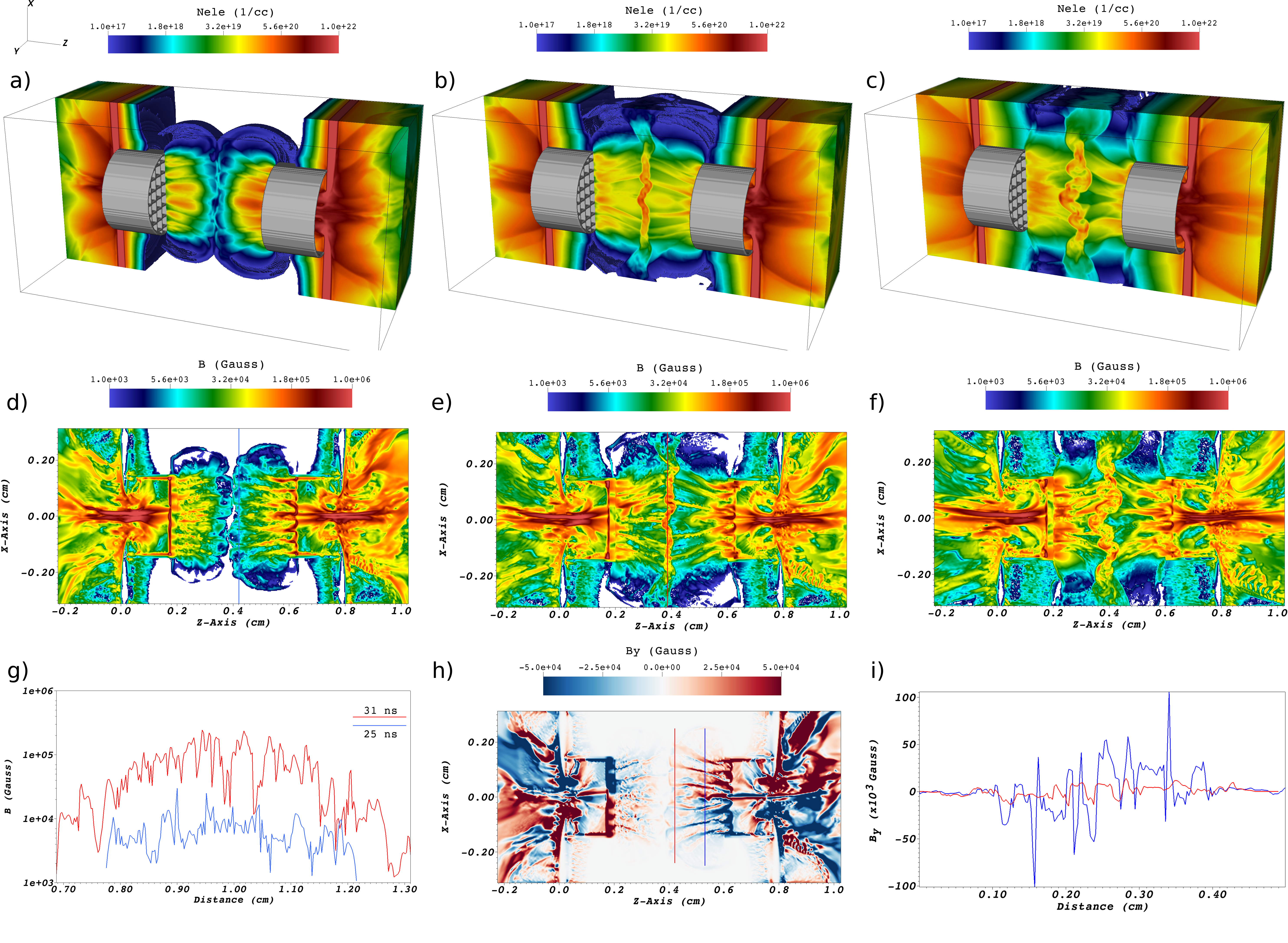
Figure 11: 3D FLASH simulations of the experiment. The temporal evolution of electron density and magnetic field strength in the FLASH simulations of the experiment, demonstrating the onset of turbulence and the turbulent dynamo amplification of the magnetic fields. a) Pseudo-color plot of electron density at $t=25\rm{ns}$, when the counter-propagating plasma flows collide. The gray contours denote the grids and cans of the assembly. b) Same as a) at $t=31\rm{ns}$, when the turbulent region is well formed. c) Same as a) at $t=37\rm{ns}$. d) Pseudo-color plot of the magnetic-field magnitude at $t=25\rm{ns}$, showing the seed fields being advected into the turbulent region. e) Same as d) at $t=31\rm{ns}$. The magnetic fields are amplified by turbulent dynamo. f) Same as d) at $t=37\rm{ns}$, i.e., at late times. g) Lineouts of magnetic field magnitude from d) and e), showing the size and fluctuations of the seed field and the amplified magnetic field. h) Pseudo-color plot of the y-component of magnetic field in the x-z plane at $t=25\rm{ns}$, showing the helical nature of the seed field. i) Lineouts of the y-component of the magnetic field from h) at different values of z, showing a decrease in the seed-field magnitude due to lateral expansion of the plasma flows.

The FLASH simulations replicate most aspects of the evolutionary history of the magnetic field that was described in the main text. More specifically, the simulated laser drive results in the generation of Biermann-battery magnetic fields, which the counter-propagating plasma flows then advect towards the center (Figure 11d). The topology of the advected fields is largely helical (Figure 11h), because the laser drive on each foil generates magnetic fields that are toroidal (24) in the plane perpendicular to the line of centers. The strength of these magnetic fields declines considerably as they are advected (Figure 11i) because the counter-propagating plasma flows expand laterally. These weak fields then serve as the seed for the fluctuation dynamo that operates in the turbulent interaction region (as claimed in the main text). The FLASH simulations show an amplification of the seed field (Figure 11e-f) from the RMS value of a few kG (blue line in Figure 11g) to RMS value of $\sim$80-130 kG and peak value of $\sim$ 300-500 kG (blue line in Figure 11g, see also Figure 8 in the main text), consistent with the experimental results.

Analysis reveals that there is an offset in time between the results of the FLASH simulations and the experimental data. We use the width of the interaction region as a function of time to determine the offset. In the FLASH simulations, we use the width of the interaction region as the distance between the locations at which the signed Mach number of the flows decreases below its signed half-maximum. For the experiment, we use the width of the interaction region determined from the X-ray self emission images, as was described previously in (23). Figure 12 shows that good agreement is obtained between the results of the FLASH simulations and the experimental data by shifting the simulations 4 ns later in time.

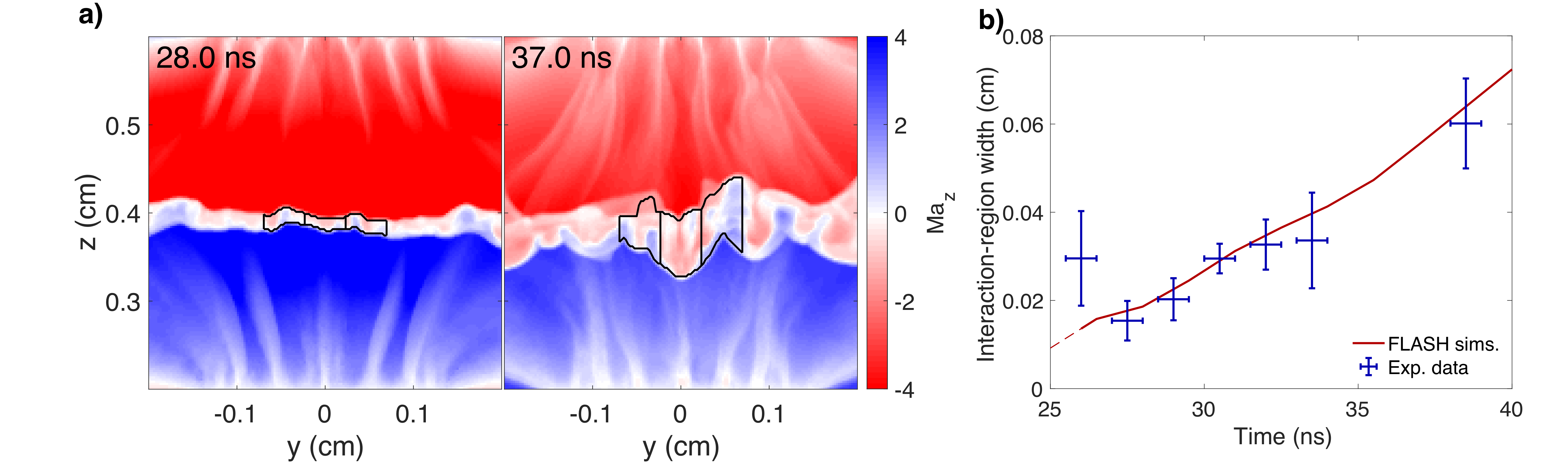
Figure 12: Calibration and validation of FLASH simulations using the width of the interaction region. We use the width of the interaction region as a function of time to calibrate the offset in time between the FLASH simulations and the experiment. a) Signed Mach number, $\mathrm{Ma}_{z}$ (defined using the $z$-component of the bulk velocity, viz., $\mathrm{Ma}_{z}\equiv\boldsymbol{u}\cdot\hat{\boldsymbol{z}}/c_{s}$) at 28.0 ns in the FLASH simulations. Examples of the adaptive fiducial volumes (central and full) at this time are also shown. b) Signed Mach number, $\mathrm{Ma}_{z}$, at 37.0 ns, in the FLASH simulations. Examples of the adaptive fiducial volumes (central and full) at this time are also shown. c) Comparison of the width of the interaction region as a function of time as given by the FLASH simulations and the experimental data. Good agreement between the results of the FLASH simulations and the experimental data is obtained by shifting the results of the simulations 4.0 ns later in time.

To enhance further the fidelity of the FLASH simulations, we incorporated the effects of the Thomson-scattering laser probe (which, according to the analysis presented in ‘Perturbative heating effects of Thomson-scattering diagnostic’, we believe to be significant). Taking into account the temporal offset, we illuminate the turbulent region at selected times of the evolution that correspond to the experimental timing of the Thomson-scattering diagnostic. The $2\omega$, $1\,\mathrm{ns}$ probe laser is configured to match the experimental configuration in terms of energy, spatial profile, and pointing properties. The Thomson-scattering beam refracts on the turbulent plasma and deposits its energy via inverse bremsstrahlung. The main effect is an increase in electron temperature (Figure 13), which is more pronounced at later times of the evolution.

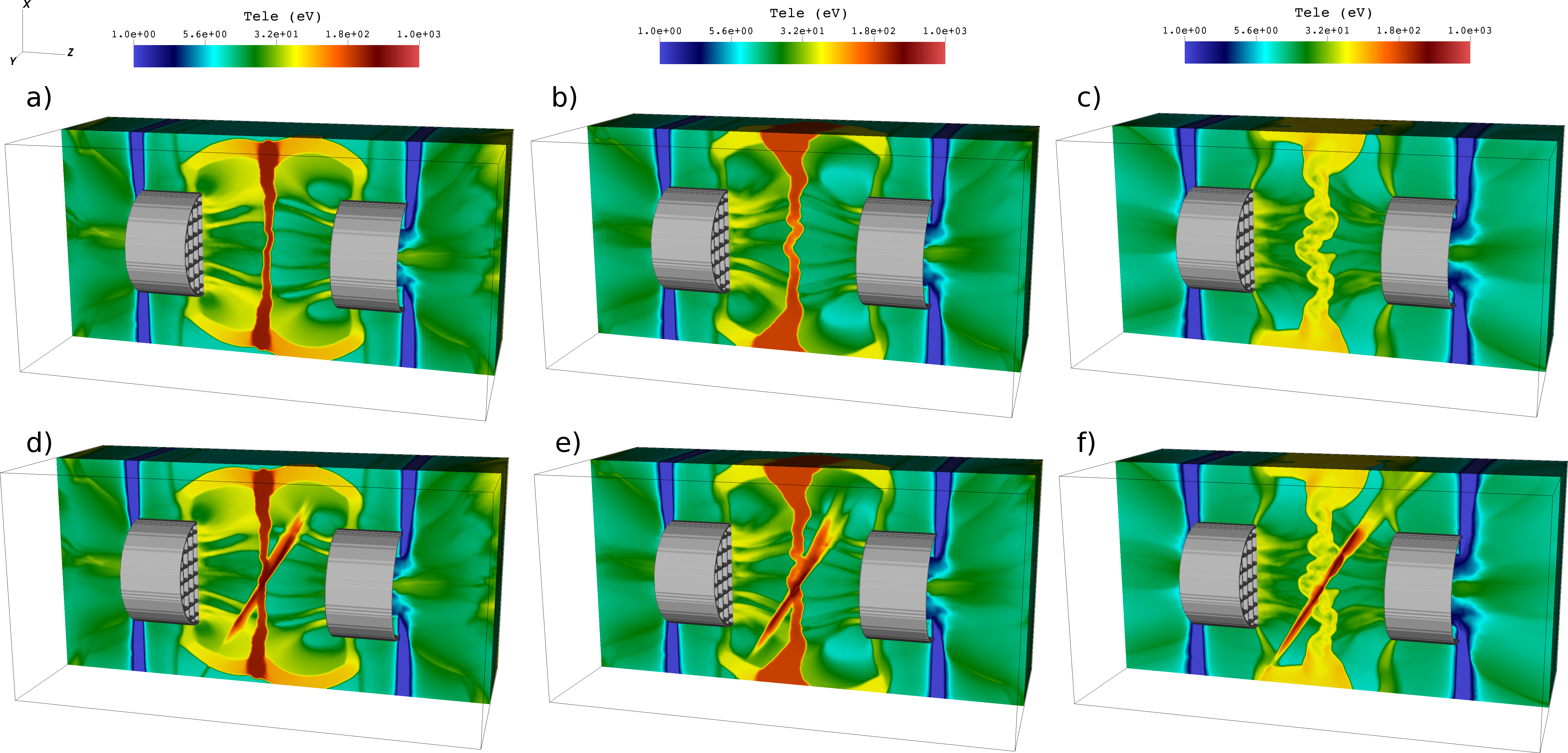
Figure 13: Modeling of the Thomson-scattering probe beam heating in the FLASH simulations. We use the FLASH code’s laser-deposition module to incorporate the effects of the Thomson-scattering probe on the turbulent plasma. The main effect of the probe is the increase of the electron temperature, predominantly at later times in the evolution of the turbulent plasma. a) Pseudo-color plot of the electron temperature at $t=27\rm{ns}$. The gray contours denote the grids and cans of the assembly. b) Same as a) at $t=31\rm{ns}$. c) Same as a) at $t=37\rm{ns}$. d) Same as a) but with the Thomson-scattering laser centered at $t=27\rm{ns}$. e) Same as b) but with the Thomson-scattering laser fired as at $t=30\rm{ns}$. f) Same as a) but with the Thomson-scattering laser fired as at $t=37\rm{ns}$.

Validation of FLASH simulations

An extensive effort was made to validate the FLASH simulations using the experimental data. To do so, we use the results of the FLASH simulations for plasma-state physical quantities in two adaptive fiducial volumes (AFVs) defined as follows. We center both AFVs on the line of centers passing through the TCC and take the width of the interaction region defined above as their dimension parallel to the line of centers. We take $500\,\mu\rm{m}$ as the dimension in the directions perpendicular to the line of centers for the first AFV (which we will refer to as the central AFV). The resulting volume is comparable to the volume sampled by the Thomson-scattering diagnostic. This volume is a cylinder with a diameter $\sim 70$-$100\,\mu\rm{m}$, and, depending on the time at which the measurement was made, a length of $\sim 300$-$1200\,\mu\rm{m}$, due to the oblique angle of the Thomson probe-beam relative to the line of centers. For the second AFV (which we will refer to as the full AFV), we take $1500\,\mu\rm{m}$ as the dimension in the directions perpendicular to the line of centers. These dimensions are more than triple the $400\,\mu\rm{m}$ grid spacing, which ensures that this AFV contains a relatively fair sample of the interaction region, making it appropriate to compare the FLASH simulation results for the plasma state properties for this AFV with the experimental data obtained using the X-ray framing camera and proton-imaging diagnostics.

Figure 14 compares the time histories obtained in the FLASH simulations for nine physical quantities with the experimental data for these quantities.

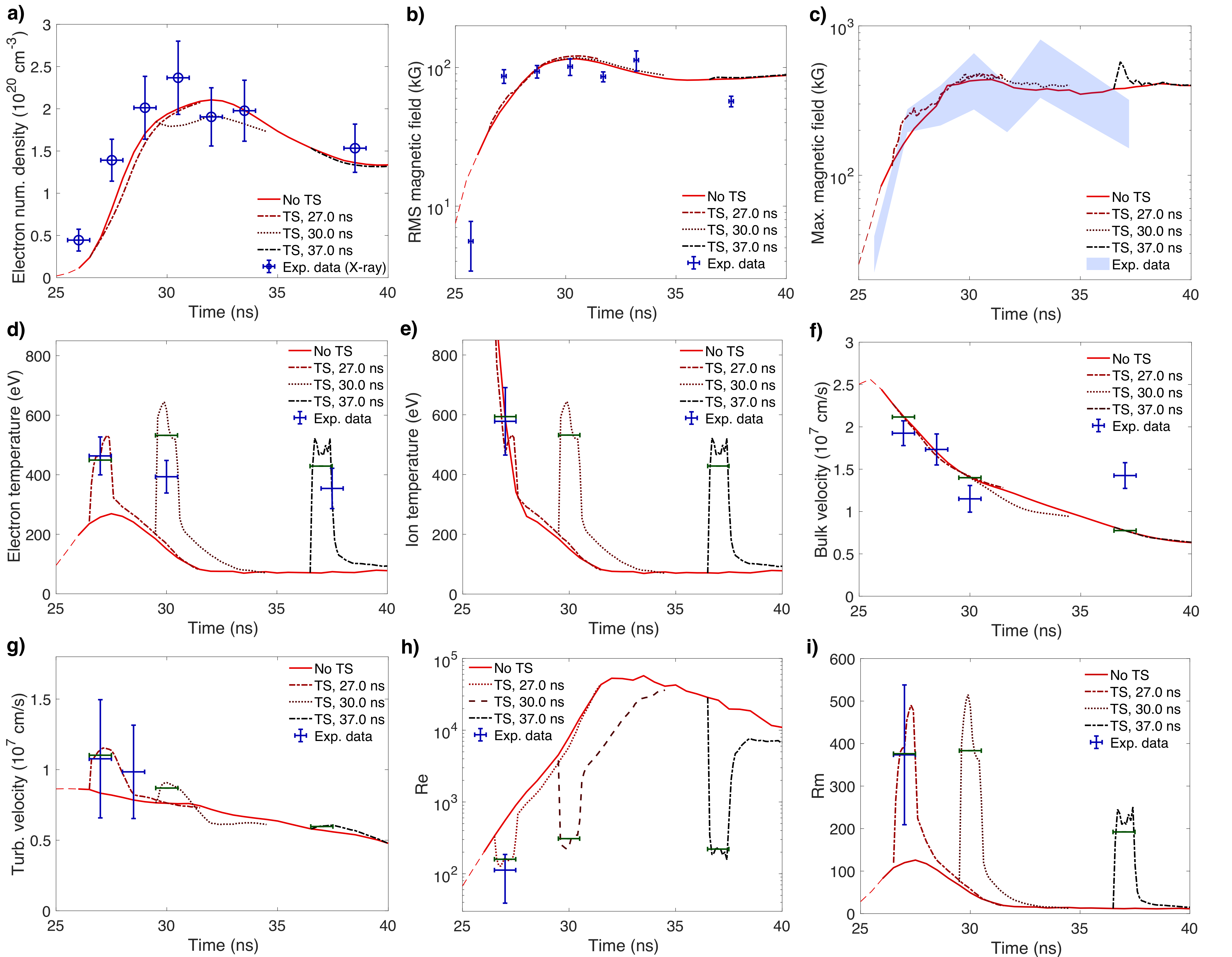
Figure 14: Further validation of the FLASH simulations using experimental data. FLASH simulation results for nine physical quantities in the interaction region are shown as a function of time with and without the heating due to the Thomson-scattering diagnostic as a result of 1-ns-long pulses centered at 27, 30 and 37 ns after the start of the laser drive. For the physical quantities measured with the Thomson-scattering diagnostic (temperatures, flow velocities, and Reynolds numbers), the results of the FLASH simulations are presented for the central adaptive fiducial volume (AFV), which is comparable to the volume sampled by the Thomson-scattering diagnostic. The results are shown as horizontal green lines whose length is equal to the duration of the 1-ns pulse of the Thomson-scattering probe beam and whose value corresponds to the mean value of the physical quantity in that time interval. The experimental data points are shown with horizontal error bars equal to the duration of the 1-ns pulse and vertical error bars corresponding to 1$\sigma$ in the physical quantity. For the other physical quantities (the electron number density measured using the X-ray imaging diagnostic and the magnetic field measured using proton imaging), the results of the FLASH simulations are presented for the full AFV. a) Electron number density. b) RMS magnetic field. c) Maximum magnetic field. d) Electron temperature. e) Ion temperature. f) Bulk velocity. g) Turbulent velocity. h) Fluid Reynolds number. i) Magnetic Reynolds number. Excellent agreement is found between the results of the FLASH simulations and the experimental data for all nine quantities, which provides further support for a 4-ns offset in time between the results of the FLASH simulations and the experimental data, and further validates the simulations.

Panels a)-c) compare the time histories of the electron number density, the RMS magnetic field and the maximum magnetic field for the full AFV (which represents a relatively fair sample of the interaction region), while panels d)-i) compare the time histories of the electron temperature, ion temperature, bulk velocity, turbulent velocity, fluid and magnetic Reynolds numbers for the central AFV (which is comparable to the Thomson-scattering diagnostic’s sampling volume). Without the heating by the Thomson-scattering probe beam, there is good agreement for all quantities save the electron and ion temperatures, which are smaller than the reported experimental values (particularly at late times). When its heating effect is incorporated, the Thomson-scattering probe beam raises the electron temperature in the Thomson-scattering volume to $500$-$600\,\rm{eV}$ for the duration of the probe beam (1 ns). This heating of the electrons has only a modest effect on the electron density, the bulk velocity and the turbulent velocity [see panels a), f) and g)] and virtually no effect on the RMS magnetic field and the maximum magnetic field [see panels b) and c)]; it does, however, have a significant effect on the fluid Reynolds number $\mathrm{Re}$, decreasing it from $\mathrm{Re}\approx 5\times 10^{3}$ - $5\times 10^{5}$ to $\mathrm{Re}\approx 200$-$300$, and on the magnetic Reynolds number $\mathrm{Rm}$ of the turbulent magnetized fluid, increasing it from $\mathrm{Rm}\approx 25$-$120$ to $\mathrm{Rm}\approx 200$-$500$, as panels h) and i) show. When the heating by the Thomson-scattering probe beam is included, the agreement is excellent in all cases, validating the simulations. Furthermore, the agreement for the electron density and the RMS magnetic field, which are physical quantities of particular interest and both of which increase rapidly, confirms that the 4 ns time offset between the FLASH simulations and the experimental data inferred from the width of the interaction as a function of time is correct.

We can also use the self-emission X-ray imaging diagnostic to provide further confirmation that the FLASH simulations are modeling the hydrodynamic physical variables of the interaction-region plasma correctly. In the main text, we establish a simple relationship between the electron density $n_{e}$, electron temperature $T_{e}$, and the measured (optical) intensity $I$ on the CCD camera associated with X-rays emitted by the plasma: $I\propto\int\mathrm{d}s\ n_{e}^{2}\hat{f}(T_{e})$, where $\hat{f}(T_{e})$ is a function defined by Eq. [2] of the main text and plotted in Figure S1b. This relationship can be used to simulate artificial X-ray images of the FLASH-simulated plasma; the resulting images are shown in Figure 15.

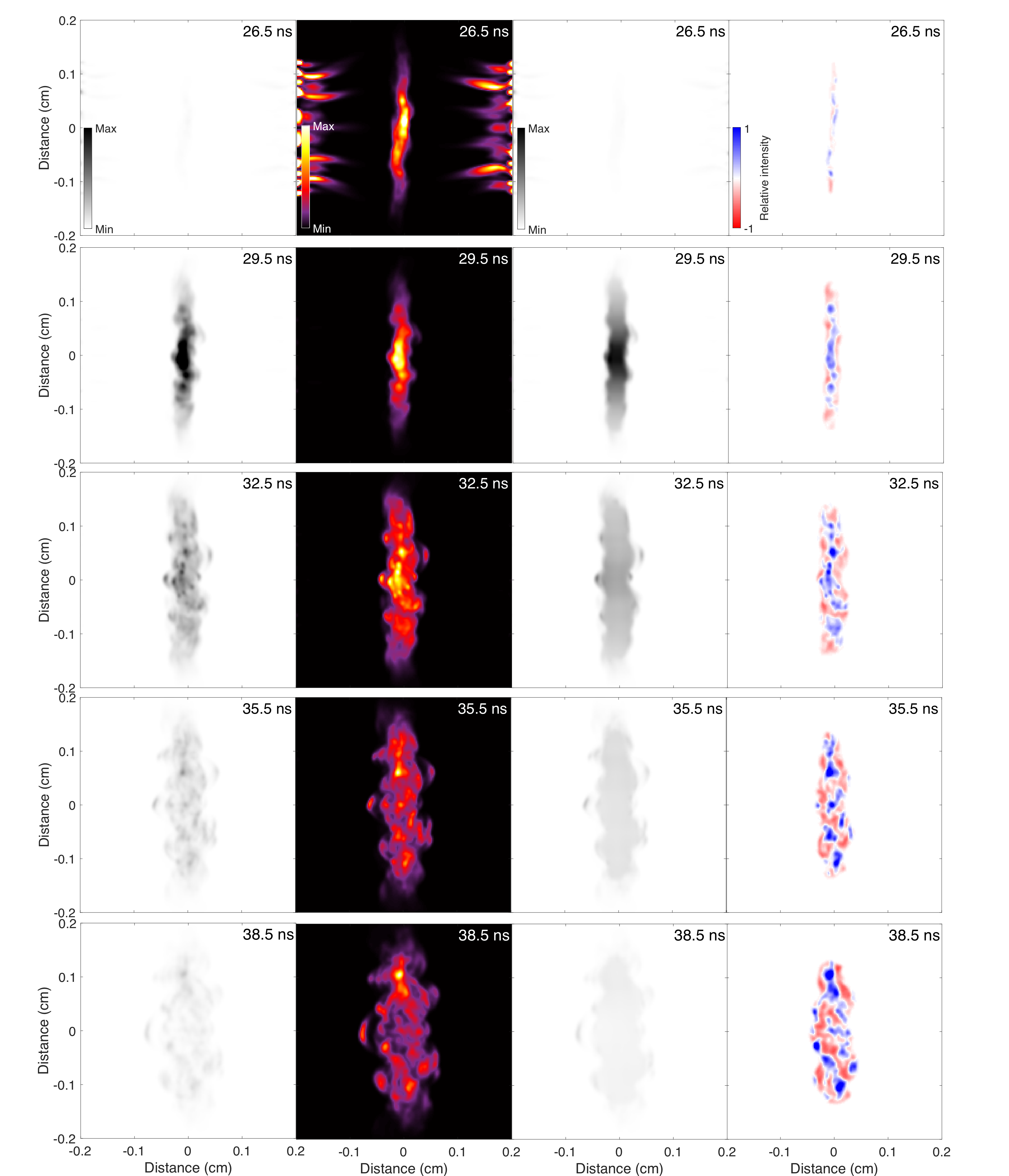
Figure 15: Self-emission X-ray images of the FLASH-simulated interaction-region plasma. First column: simulated ‘absolute’ X-ray intensity images, normalized to the maximum count value associated with the interaction-region plasma across all of the images (which is realized at $t=29.5$ ns). The 50 $\mu$m resolution limit of the experimental X-ray images is incorporated into the simulated images via a convolution with a two-dimensional Gaussian filter of the appropriate width. Second column: X-ray intensity images normalized by the maximum pixel value in each image. Third column: mean emission profiles calculated from the far-left column; the gray-scale map is the same as in the far-left images. Fourth column: relative X-ray intensity map calculated from the mean emission profile. Fluctuations with a positive value with respect to the mean intensity are denoted in blue, negative in red, with maximum and minimum values set at $\pm 100\%$ of the mean value.

The agreement (both qualitative and quantitative) between the evolution of the FLASH images and those from the experiment is excellent: at $t=26.5$ ns, the emission from the interaction region is comparable to that of the grid jets, and is considerably weaker than 1.5 ns later; peak emission is at 29.5 ns; then the total emission drops off considerably by $t=38.5$ ns. As a further validation, the synthetic X-ray images derived from the FLASH simulations were analyzed using the same procedure that was applied to the experimental images: we extract mean-emission and relative-intensity maps, and then evaluate the RMS of the latter. As shown in Figure 4c of the main text, the RMS of relative fluctuations derived from the synthetic images evolves similarly to the RMS derived from the experimental images (save perhaps at late times). In summary, the results of the simulated X-ray self-emission images provide additional validation of the accuracy of the hydrodynamic modeling of the FLASH simulations.

Evolution of the interaction-region plasma in the FLASH simulation

Figure 16 shows the time histories of eight physical quantities in the FLASH simulations for the full AFV (which represents a relatively fair sample of the interaction region).

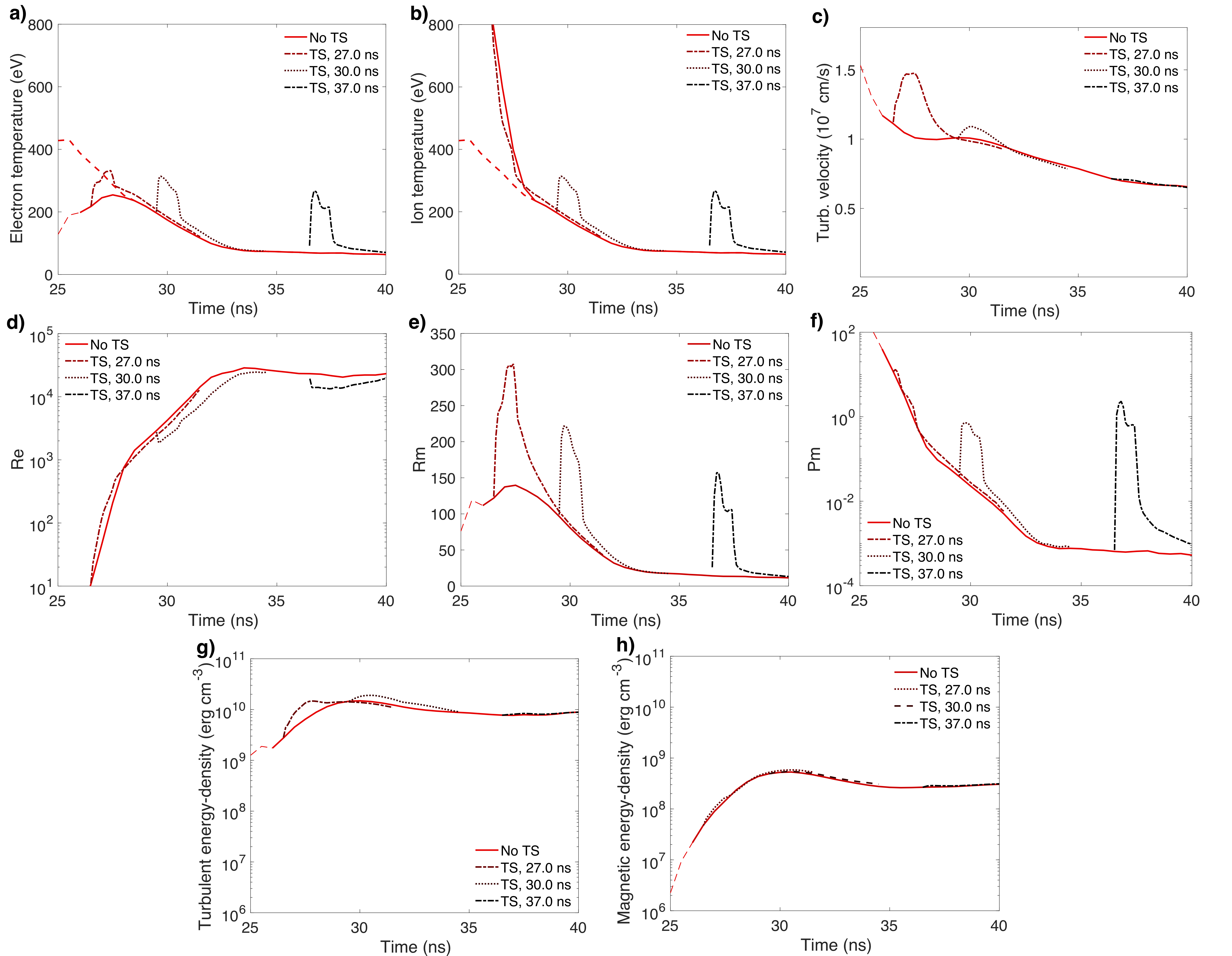
Figure 16: Evolution of physical quantities in the FLASH simulations. FLASH simulation results are shown as a function of time for eight physical quantities, averaged over the full adaptive fiducial volume for no heating and for heating by the 1-ns-long Thomson-scattering probe beam at times centered at 27, 30 and 37 ns after the start of the laser drive. a) Electron temperature. The thick dashed red line depicts the electron-temperature history under the assumption of equal and ion temperatures in the FLASH simulations, but conserving total thermal energy of the plasma. b) Ion temperature. c) Turbulent velocity. d) Turbulent fluid Reynolds number. e) Turbulent magnetic Reynolds number. f) Magnetic Prandtl number. g) Turbulent-energy density. h) Magnetic-energy density.

Results are shown for the case of no heating and when some heating occurs as a result of 1-ns-long Thomson-scattering probe beam pulses centered at 27, 30 and 37 ns after the start of the laser drive. These figures illustrate two key features of the experiment.

First, the rapid collisional shock heating that occurs immediately after the interaction region forms causes the initial electron temperature to exceed 250 eV and the initial ion temperature to exceed 600 eV. This simultaneously decreases the resistivity and increases the viscosity, leading to $\mathrm{Pm}=\mathrm{Rm}/\mathrm{Re}>1$ at early times. We note that the exceptionally high ion temperatures (> 1 keV) obtained in the simulations just after the interaction region forms are not likely to be physical; at these early times, the plasma is not fully collisional, and thus the collisional electron-ion heating model assumed in a one-fluid MHD code such as FLASH (which presumes that ions are viscously heated predominantly over electrons) is not strictly applicable. As a comparative reference, panels a) and b) of Figure 16 show an alternative evolutionary history of the electron and ion temperatures derived under two assumptions: that evolution of the total thermal energy in the plasma is captured accurately by the FLASH simulations, but with fixed $T_{e}=T_{i}$ at all times. In this alternative model, we find that the electron and ion temperatures just after the interaction region forms (at $t$ = 25.5 ns) are $T_{e}=T_{i}\approx 450\,\mathrm{eV}$. This is in close agreement with the reported experimental values, suggesting that as the interaction region is forming, collisional electron heating could be significant. Such an effect has indeed been seen previously in laser-plasma experiments involving counter-streaming CH plasma jets (25).

Secondly, the Thomson-scattering probe beam heating has a non-trivial effect on the interaction-region plasma’s dynamics, particularly at late times. For the earliest time at which the Thomson-scattering beam heating was introduced in the FLASH simulations ($t$ = 27 ns), the electron temperature and turbulent velocity are increased by $\sim 30\%$ over their unperturbed values [see panels a) and c)] in the full AFV, resulting in an increased $\mathrm{Rm}$ [see panel e)]. At later times, the probe-beam heating has an increasingly significant effect on the electron and ion temperatures [see panel b)], decreasing the fluid Reynolds number $\mathrm{Re}$ [see panel d)] and increasing the magnetic Reynolds number $\mathrm{Rm}$ of the turbulent plasma. Overall, the heating has only a modest effect on the turbulent kinetic energy density [see panel g)] and virtually no effect on the magnetic-energy density [see panel h)]. Panel f) shows that $\mathrm{Pm}>1$ during the 1-ns duration of the Thomson-scattering probe beams at later times. We emphasize that the initial amplification of the magnetic field always occurs in the $\mathrm{Pm}>1$ regime, irrespective of the Thomson-scattering probe beam heating.

The growth rate of the magnetic field in the FLASH simulations

Figure 17 compares (1) the rate of growth of the magnetic energy in the interaction region (subtracting the magnetic energy advected into it by the two plasma flows and adding the magnetic energy advected out of it by the bulk flow perpendicular to the line of centers in that time period), (2) the rate at which magnetic energy is advected out of the interaction region by the bulk flow perpendicular to the line of centers, (3) the turbulent eddy turnover rate at the outer scale $L=400\,\mu\mathrm{m}$ in the interaction region given by the validated FLASH simulations, and (4) the RMS rate of strain of the FLASH-simulated velocity field (a fifth quantity, the RMS rate of perpendicular strain of the component of FLASH-simulated velocity parallel to the line of centers, is also shown, and is discussed in the next section).

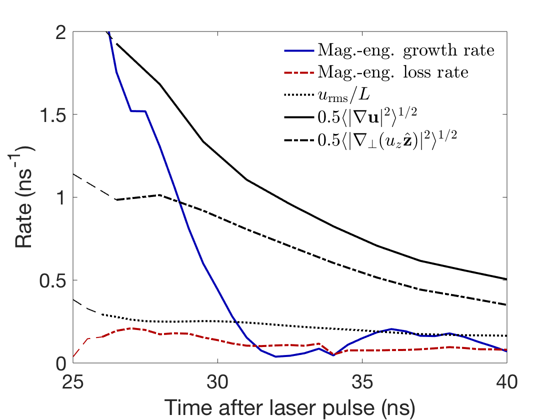
Figure 17: FLASH simulation results for the rates of change of five physical quantities in the interaction region. Shown are the FLASH simulation results for the rate of magnetic-energy growth $\mathrm{d}\log{E_{B}}/\mathrm{d}t$ (which we define as the increase in the magnetic energy in a given time period, subtracting the magnetic energy advected in by the two plasma flows and adding the magnetic energy advected out by the bulk flow perpendicular to the line of centers in the same time period), the magnetic-energy loss rate due to advection out by the bulk flow perpendicular to the line of centers (which is determined by calculating the flux of magnetic energy through the four perpendicular faces of the volume being sampled), the turbulent eddy turnover rate at the outer scale $L=400\,\mu\mathrm{m}$, the RMS rate of strain [defined here as $\langle|\nabla\boldsymbol{u}|^{2}\rangle^{1/2}$; the 0.5 factor is introduced for convenience of plotting], and the RMS rate of perpendicular strain of the component of velocity parallel to the line of centers [defined as $\langle|\nabla u_{z}\hat{\boldsymbol{z}}|^{2}\rangle^{1/2}$] – all for the full AFV.

The results for all four quantities are for the full AFV. Figure 17 shows that, at early times, the growth rate of the magnetic energy is much greater than the rate at which the magnetic field energy is advected out of the interaction region, while at late times, the former is comparable to, or somewhat larger than, the latter.

Of particular interest is that, at early times, the magnetic energy grows at a rate $\gamma\approx 2\times 10^{9}$ s^-1 (which is equivalent to a growth time of 0.5 ns). This rate, which is similar to that obtained experimentally, is comparable to the RMS rate of strain, but is ${\sim}5$–$10$ times larger than the outer-scale eddy turnover rate $\gamma_{\rm L}={u_{\rm rms}}/{L}\approx 2.5\times 10^{8}$ s^-1, where $L$ is the outer scale of the turbulence and $u_{\rm rms}$ is the RMS velocity at that scale. This rate is equivalent to a growth time $\tau_{L}\approx 4$ ns. As discussed in the main text, based on periodic-box MHD simulations of the fluctuation dynamo at comparable magnetic Reynolds and magnetic Prandtl numbers (7, 26), the growth rate of the magnetic energy is expected to be smaller than what we see here. This suggests that there is another growth mechanism also at play (see next section).

The role of directed shear flows in our experiment

In the main text, we suggest that the interaction between stochastic motions and directed shear flows in the interaction-region plasma could explain the fast growth of the magnetic field that is observed in the experiment and in FLASH simulations; here, we use the latter to help provide evidence for this claim.

Figures 18 and 19 show the velocity field in the FLASH simulations at three times during the 6 ns time interval after the interaction region forms.

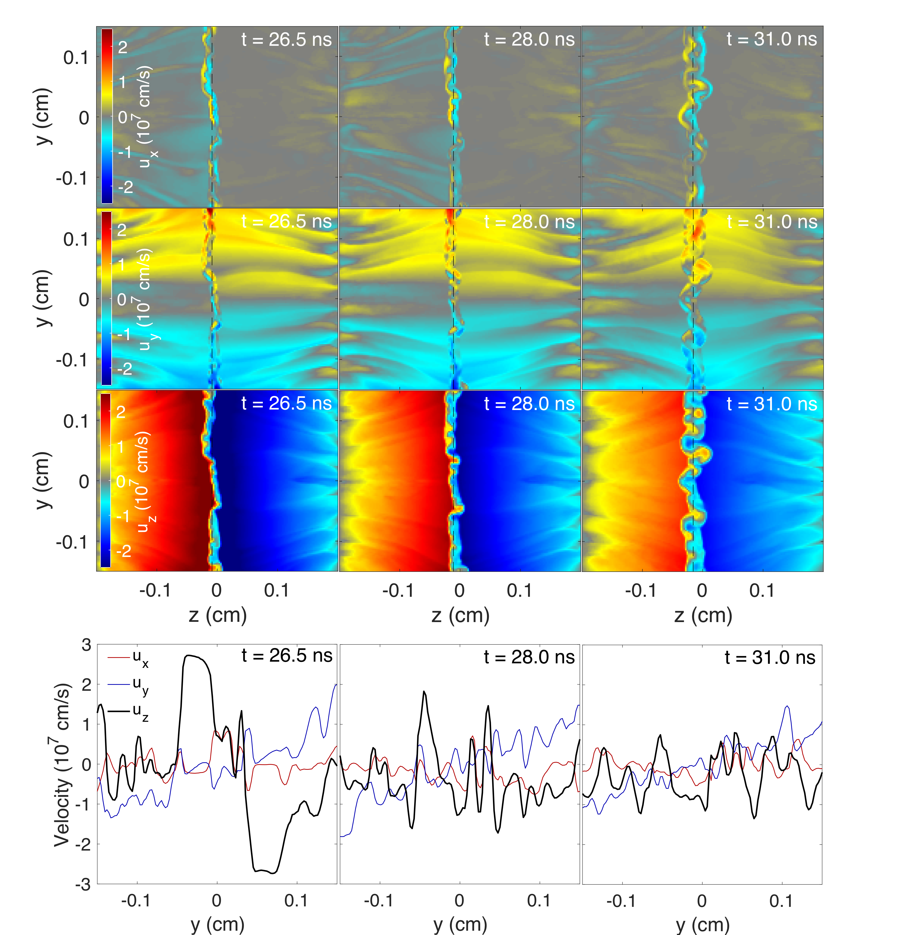
Figure 18: The velocity field in the FLASH simulations. Top grid: pseudo-color two-dimensional slice plots [in the ($y$,$z$) plane) of the three components of velocity in the FLASH simulations at $t=26.5$ ns (left column), $t=28.0$ ns (middle column) and $t=31.0$ ns (right column). Bottom row: lineouts (in the $y$ direction) of the three components of velocity, at $t=26.5$ ns (left column), $t=28.0$ ns (middle column) and $t=31.0$ ns (right column). The lineouts are taken at the positions indicated on the top grid of slice plots by a dashed line.

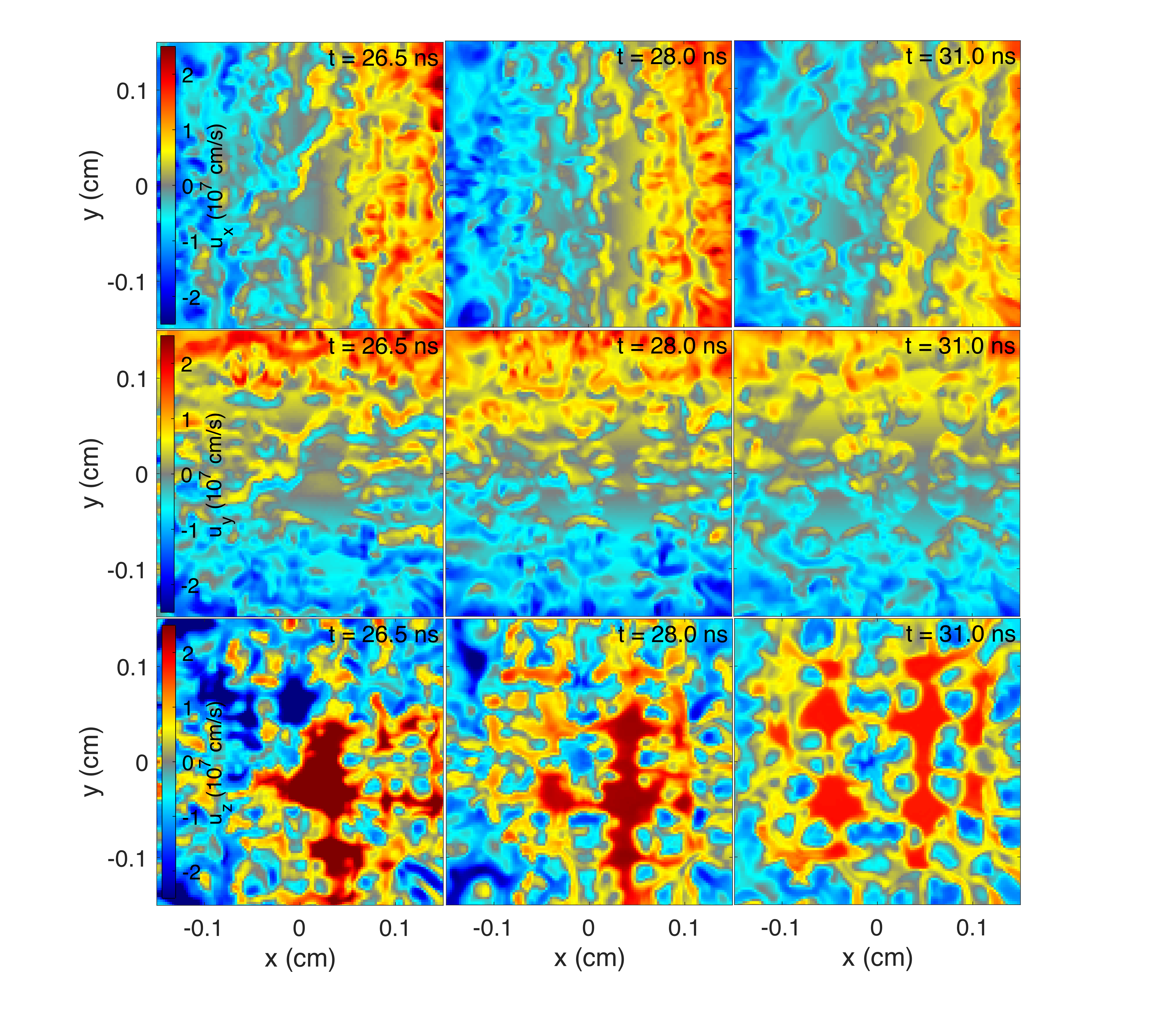
Figure 19: Perpendicular slices of the velocity field in the FLASH simulations. Pseudo-color two-dimensional slices plots [in the ($x$,$y$) plane) of the three components of velocity in the FLASH simulations at $t=26.5$ ns (left column), $t=28.0$ ns (middle column) and $t=31.0$ ns (right column). The slices are taken at the position on the $z$ axis coincident with the lineouts shown in Figure 18.

The presence of directed shear flows in addition to stochastic motions is most clearly illustrated by taking lineouts of the velocity field in the plane of the interaction-region plasma (see Figure 18, bottom row): changes in velocity $\Delta u_{z}\approx 200$–$300$ km$\,\mathrm{s}^{-1}$ are seen in the component of velocity ($u_{z}$) parallel to the line of centers over a characteristic reversal scale $\Delta x_{\perp}\approx 75$–$125\;\mu$m in the directions that are perpendicular to the line of centers. By comparison, changes in the other two velocity components over the same length scale are much smaller ($\Delta u_{x},\Delta u_{y}<100$ km$\,\mathrm{s}^{-1}$). These shear flows are seen across the whole perpendicular plane of the interaction-region plasma (see Figure 19).

The physical origin of these directed shear flows is the asymmetry of the counter-propagating plasma “fingers”, or jets, originating from the offset of the two grids. In perpendicular spatial locations coincident with the holes in grid A, the density of the jets originating from grid A is much higher than grid B; an analogous statement holds for spatial locations coincident with the holes in grid B. On the other hand, the $u_{z}$ component of velocity is close to uniform across each jet (see Figure 18, bottom row of top grid). Conservation of momentum therefore dictates that when the jets collide, the bulk velocity of plasma in these perpendicular spatial locations will be directed towards grid B or grid A, respectively. The counter-propagating, interleaving jets will shear, forming shear layers along the line of centers (i.e., the z axis in the FLASH simulations). Even though the Kelvin-Helmholtz (KH) instability will likely act to destabilize these shears (see next section), the continual re-supply of plasma by the plasma jets helps to sustain these flows for at least one driving-scale eddy turnover time (see Figure 18, final column).

Given the parameter regime of our experiment – specifically, the relatively large viscosity in the interaction-region plasma at times $t\leq 27\,\mathrm{ns}$ ($\nu\approx 3\times 10^{3}\;\mathrm{cm}^{2}\,\mathrm{s}^{-1}$) – the FLASH simulations resolve the transverse scale of these shear layers, apart from at very early times in the experiment. Consider the evolution of a simple unsteady viscous shear layer with $\boldsymbol{u}=u_{z}(y,t)\hat{\boldsymbol{z}}$. The flow profile $u_{z}(y,t)$ in such a layer is given by (27)

$$u_{z}(y,t)=\frac{\Delta u_{z}}{2}\,\mathrm{erf}{\left(\frac{y}{\sqrt{4\nu t}}\right)}\approx\frac{\Delta u_{z}}{2}\tanh{\left(\frac{y}{\sqrt{\pi\nu t}}\right)},$$ (13)

where the second expression will be used in the analysis of the KH instability in the next section. A reasonable estimate for the width of the shear layer at time $\Delta t$ after it forms is therefore twice the viscous scale length, viz., $\Delta x_{\perp}\approx 2\sqrt{\pi\nu\Delta t}$. Conservatively choosing $\Delta t\gtrsim 1$ ns (corresponding to the relevant time delay after the interaction-region formation at $t=25$–$26$ ns), we find $\Delta x_{\perp}\gtrsim 60\;\mu$m. The resolution of the FLASH simulations is $\Delta x_{\rm res}=25\;\mu$m, implying that such reversals are indeed captured in the simulations. As a result, the strain rate of the shear flow in the experiment can be reasonably estimated as being similar to that found in the simulations. Note that, because $\nu$ decreases considerably as the plasma’s ions cool, the shear layers are unlikely to broaden further due to viscous effects after $t\approx 27$ ns. Therefore, in the initial phases of the magnetic-field evolution within the turbulent interaction-region plasma, we have sustained, directed shear flows, which contribute to the total rate of strain that drives the dynamo action responsible for the magnetic-field amplification.

More quantitatively, at $t\sim 27$ ns the strain rate of the directed shear flows $S\equiv\langle|\nabla_{\perp}(u_{z}\hat{\boldsymbol{z}}|^{2}\rangle^{1/2}$ is $S\approx\Delta u_{z}/\Delta x_{\perp}\approx 2\times 10^{9}\;\mathrm{s}^{-1}$ (see also Figure 17, where the exact value of this quantity for the central AFV is calculated). This is ${\gtrsim}\,50\%$ of the total measured RMS rate of strain shown in Figure 17, supporting the claim that these directed flows contribute to the fast amplification rate of the magnetic field. It becomes apparent that the fluctuation dynamo realized in our experiment is enhanced by shear dynamo [see (28) and references therein] at early times. This is further evidenced by the time evolution of the rate of strain $\gamma_{\ell_{\nu}}\sim\mathrm{Re}^{1/2}u_{\rm rms}/L$ of viscous-scale turbulent eddies, which is anticipated to be proportional to the growth rate of the magnetic field if fluctuation dynamo were the only mechanism at play. At early times, this is not the case. In many astrophysical cases, such as the merger of galaxies and the growth of galaxies clusters through cluster mergers, the capturing of groups and the infall of filaments, strong shear flows are present (29). In this sense, the experiments we have conducted could be more relevant to the astrophysical case than previous numerical simulations of turbulent dynamo, which typically generate the turbulent spectrum by an isotropic forcing mechanism (26) (although whether this is actually the case ultimately depends on the true magnitude of $\mathrm{Re}$ in astrophysical systems – a quantity of some uncertainty (30) – as well as the properties of astrophysical analogues of colliding jets).

In spite of the important role of the directed shear flows, the presence of the stochastic fluid motions – which are responsible for fluctuation dynamo in both experiments and simulations – is essential. This is because a quasi-2D unidirectional shear flow cannot drive sustained amplification of magnetic fields by itself. This can be demonstrated by considering the MHD induction equation for a velocity field of the form $\boldsymbol{u}(\boldsymbol{r})=U(x,y)\hat{\boldsymbol{z}}$; writing out separately the induction equation’s components perpendicular and parallel to $\hat{\boldsymbol{z}}$, we have

$$\frac{\partial\boldsymbol{B}_{\perp}}{\partial t}+U\frac{\partial\boldsymbol{B}_{\perp}}{\partial z} = \eta\nabla^{2}\boldsymbol{B}_{\perp}\,,$$ (14)

$$\frac{\partial B_{z}}{\partial t}+U\frac{\partial{B}_{z}}{\partial z} = \boldsymbol{B}_{\perp}\cdot\nabla_{\perp}U+\eta\nabla^{2}{B}_{z}\,,$$ (15)

where $\nabla\equiv\partial/\partial\boldsymbol{r}$. It follows that the shear flow cannot stretch $\boldsymbol{B}_{\perp}$, which must, therefore, decay on resistive timescales. The remaining component of the magnetic field, $B_{z}$, can be amplified transiently, but must eventually also decay, because $\boldsymbol{B}_{\perp}$ does. If, on the other hand, $\boldsymbol{u}(\boldsymbol{r})=U(x,y)\hat{\boldsymbol{z}}+\delta\boldsymbol{u}(\boldsymbol{r})$, where $\delta\boldsymbol{u}(\boldsymbol{x})$ is some stochastic component of the velocity, the MHD induction equation instead becomes

$$\frac{\partial\boldsymbol{B}_{\perp}}{\partial t}+U\frac{\partial\boldsymbol{B}_{\perp}}{\partial z}+\delta\boldsymbol{u}\cdot\nabla\boldsymbol{B}_{\perp} = \boldsymbol{B}\cdot\nabla\delta\boldsymbol{u}_{\perp}+\eta\nabla^{2}\boldsymbol{B}_{\perp}\,,$$ (16)

$$\frac{\partial B_{z}}{\partial t}+U\frac{\partial{B}_{z}}{\partial z}+\delta\boldsymbol{u}\cdot\nabla{B}_{z} = \boldsymbol{B}_{\perp}\cdot\nabla_{\perp}U+\boldsymbol{B}\cdot\nabla\delta{u}_{z}+\eta\nabla^{2}{B}_{z}\,.$$ (17)

It is then possible for stochastic motions in the perpendicular direction to stretch $\boldsymbol{B}$, and thus couple the growth of $\boldsymbol{B}_{\perp}$ and $B_{z}$. In our experiment, the perpendicular stochastic motions originate from the complex perpendicular flow profiles arising due to the interaction between jets extending from adjacent grid holes, and the aforementioned KH instabilities (which grow at a rate greater than the eddy turnover rate at the outer scale, as shown in the next section).

In short, the dynamo action realized in our experiments amplifies the magnetic field at a rate consistent with the total rate of strain predicted by the validated FLASH simulations. A significant component of that strain rate is attributed to the presence of multiple directed shear flows, which are not scale separated from the turbulence. The amplification mechanism is therefore consistent with a fluctuation dynamo that is enhanced by a shear dynamo at early times. This hybrid configuration reconciles the fast amplification we obtain with respect to periodic-box MHD simulations, and may be more relevant for realistic astrophysical scenarios in the ICM where shear is present.

The Kelvin-Helmholtz instability in our experiment

In this section, we estimate the growth rate of the KH instability associated with the directed shear flows in the interaction-region plasma, and show that motions perpendicular to the shear flows should grow at a greater rate than the outer-scale eddy-turnover rate.

The magnetic fields in the interaction region are not dynamically important initially, so we focus on the hydrodynamic KH instability. The theory of the hydrodynamic KH instability is well established. In an inviscid fluid containing a simple shear layer with a discontinuous velocity profile (change in velocity $\Delta u_{z}$), the wavevector of the fastest-growing modes is parallel to the fluid velocity, and the linear growth rate $\gamma_{\mathrm{KH},0}$ of such modes as a function of their wavenumber $k$ is given by (31)

$$\gamma_{\mathrm{KH},0}=\frac{1}{2}k\Delta u_{z}.$$ (18)

In a viscous fluid, a reduction of the growth rate is caused by the finite width of the shear layer (32). As an example, (33) show that, for a hyperbolic-tangent profile with a characteristic reversal scale $\Delta x_{\perp}$, the peak growth (for $M_{s}\equiv\Delta u_{z}/c_{\rm s}\approx 1$, as in our experiment) occurs at the wavenumber $k_{\rm max}$ satisfying $k_{\rm max}\Delta x_{\perp}\approx 0.8$, with

$$\gamma_{\rm max}\approx 0.14{\frac{\Delta u_{z}}{\Delta x_{\perp}}}\approx 0.2k_{\rm max}\Delta u_{z}\approx 0.4\gamma_{\mathrm{KH},0}(k_{\rm max}).$$ (19)

The finite width of the shear layer suppresses growth for wavenumbers greater than $k_{c}\approx 1.8\Delta x_{\perp}^{-1}$. From the FLASH simulations, we estimate $\Delta u_{z}\approx 250\;\mathrm{km}\,\mathrm{s}^{-1}$ and $\Delta x_{\perp}\approx 60\;\mu$m at $t\approx 27$ ns. We therefore determine from Eq. [19] that $\gamma_{\rm max}\approx 6\times 10^{8}\;\mathrm{s}^{-1}>L/u_{\rm rms}$ at $k_{\rm max}\approx 100\;\mathrm{cm}^{-1}$. This confirms our original claim that the KH growth time is comparable to the outer-scale eddy-turnover rate.

For completeness, we discuss a few caveats relating to this calculation, as well as an important implication. First, we have assumed that the KH growth rates of a finite initial perturbation of a shear layer superimposed on a turbulent environment can be estimated using linear theory derived for a simple shear profile. This assumption is not justified a priori – but it seems reasonable to assume that the true growth rate is not vastly different from our estimate. Secondly, our estimate also assumes that the shear layer driving the instability has a constant thickness: if instead the initial shear layers that develop in the interaction-region plasma have a smaller reversal scale, then both the KH-instability growth rate and the wavenumber of the fastest-growing KH mode could be considerably larger. Thirdly, for the parameters assumed here, we obtain the (perhaps surprising) result that the fastest-growing mode is at a wavenumber corresponding to the grid periodicity ($k_{\rm max}\approx 2\pi/L$), rather than at smaller scales. This finding, which follows directly from the finite width of the shear layers, suggests that the effect of the KH instability on the velocity field is to convert the energy in the shear flows into outer-scale motions; in other words, our characterization in the main paper of the grid periodicity as the ‘driving scale’ is an appropriate one. Note, however, that the most unstable KH modes have a half-wavelength ${\sim}L/2$ which is a (large) order-unity factor (${\sim}4$) greater than the characteristic reversal scale of the shears $\Delta x_{\perp}$, and so $\Delta u_{z}/\Delta x_{\perp}\approx 8u_{\rm rms}/L$; this explains why the typical shear in the directed flows is measurably greater than the outer-scale eddy-turnover rate

Dynamical significance of the magnetic fields in the FLASH simulations

The red curves in Figure 20a show the overall ratio of the sum of the magnetic energy in all of the cells and the sum of the turbulent kinetic energy in all of them as a function of time in the full AFV for the validated FLASH simulations.

Figure 20: Some properties of the magnetic energy relative to the turbulent kinetic energy as a function of time in the adaptive volume in the interaction region from the FLASH simulations. a) Global ratio of the total magnetic energy and the total turbulent kinetic energy (red lines) and average of the local ratios of the magnetic energy and the turbulent kinetic energy. b) Probability density functions for the ratio of the magnetic energy and the turbulent kinetic energy in the spatial cells in the full adaptive volume at different times during the experiment.

The ratio rises rapidly at first and then increases at a slower rate, reaching a value ${\sim}3$–$5\%$ at 40 ns.

As discussed in the main text, the small value of global magnetic-kinetic energy ratio is quite small can, in fact, still be consistent with the magnetic field being dynamically significant in the FLASH simulations. We illustrate this in two ways. Firstly, the magnetic-kinetic energy ratio attains larger values locally than globally: the blue curves in Figure 20a show the sum of the ratio of the magnetic energy and the turbulent kinetic energy in each spatial cell in the full adaptive fiducial volume. The former is approximately five times larger than the latter. More directly, Figure 20b shows the probability density function of the ratio of the magnetic energy and the turbulent kinetic energy in each spatial cell. It reveals that at later times, the ratio of the magnetic energy and the turbulent kinetic energy is comparable to, and even greater than, unity in some spatial cells, and, therefore, that the magnetic field is dynamically important at these locations in the interaction region.

Confirming the difference in magnetic-field integral scale between FLASH simulations and experiment by direct analysis of proton images

In the main text, we claim that the integral scale $L_{\rm int,B}$ of the magnetic fields obtained from the experimental proton-imaging data was a factor of a few larger than the equivalent values obtained from the FLASH (and other MHD) simulations, and also that the amount of power in the measured magnetic-energy energy spectrum at wavenumbers close to the driving wavenumber was significantly larger than anticipated from simulations. However, as mentioned in the main text, it is known that the accurate recovery of the magnetic-energy spectrum from proton images via a (path-integrated) field-reconstruction algorithm is only possible in a certain imaging-parameter regime: specifically, when the magnetic field strength $B$ of magnetic structures with correlation scale $\ell_{B}$ satisfies

$$B\lesssim 125\left[\frac{\mathcal{M}}{\mathcal{M}-1}\right]\left[\frac{\mu_{c}}{1/2}\right]\left[\frac{W_{p}(\mathrm{MeV})}{15.0\,\mathrm{MeV}}\right]^{1/2}\left[\frac{r_{i}(\mathrm{cm})}{1\,\mathrm{cm}}\right]^{-1}\left[\frac{\ell(\mathrm{cm})}{0.01\,\mathrm{cm}}\right]^{1/2}\left[\frac{l_{p}(\mathrm{cm})}{0.05\,\mathrm{cm}}\right]^{-1/2}\mathrm{kG}\,,$$ (20)

where $\mathcal{M}$ is the magnification of the imaging set-up, $W_{p}$ the proton energy, $\mu_{c}$ the contrast parameter, and $r_{i}$ the distance between the magnetic fields being imaged and the proton source (34). In this experiment, we find this condition is only marginally satisfied for the largest magnetic structures; it is therefore the case that the spectrum recovered at wavenumbers $k\gtrsim 3\pi/L_{\rm int,B}$ will be inaccurate (viz., suppressed compared to the true spectrum) if the true spectrum follows a power law shallower than $k^{-2}$. To confirm that the difference in integral scales is nevertheless a physical result, we calculate the one-dimensional spectrum of flux variations in the experimental proton images, and then re-apply the analysis to simulated proton images of the FLASH-simulated magnetic fields. Working with the proton-imaging data directly removes any possibility that it is the algorithm recovering the path-integrated fields that causes the discrepancy in characteristic field scale. Figure 21 shows the results of such an analysis at three different times after stochastic fields have been amplified in the experiment. At all times, an absence of power in the FLASH-simulated relative-flux spectra at wavenumbers $k\lesssim 25\,\mathrm{mm}^{-1}$ is indeed observed. Thus, the discrepancy between the spatial structure of the experimentally measured and simulated fields is real.

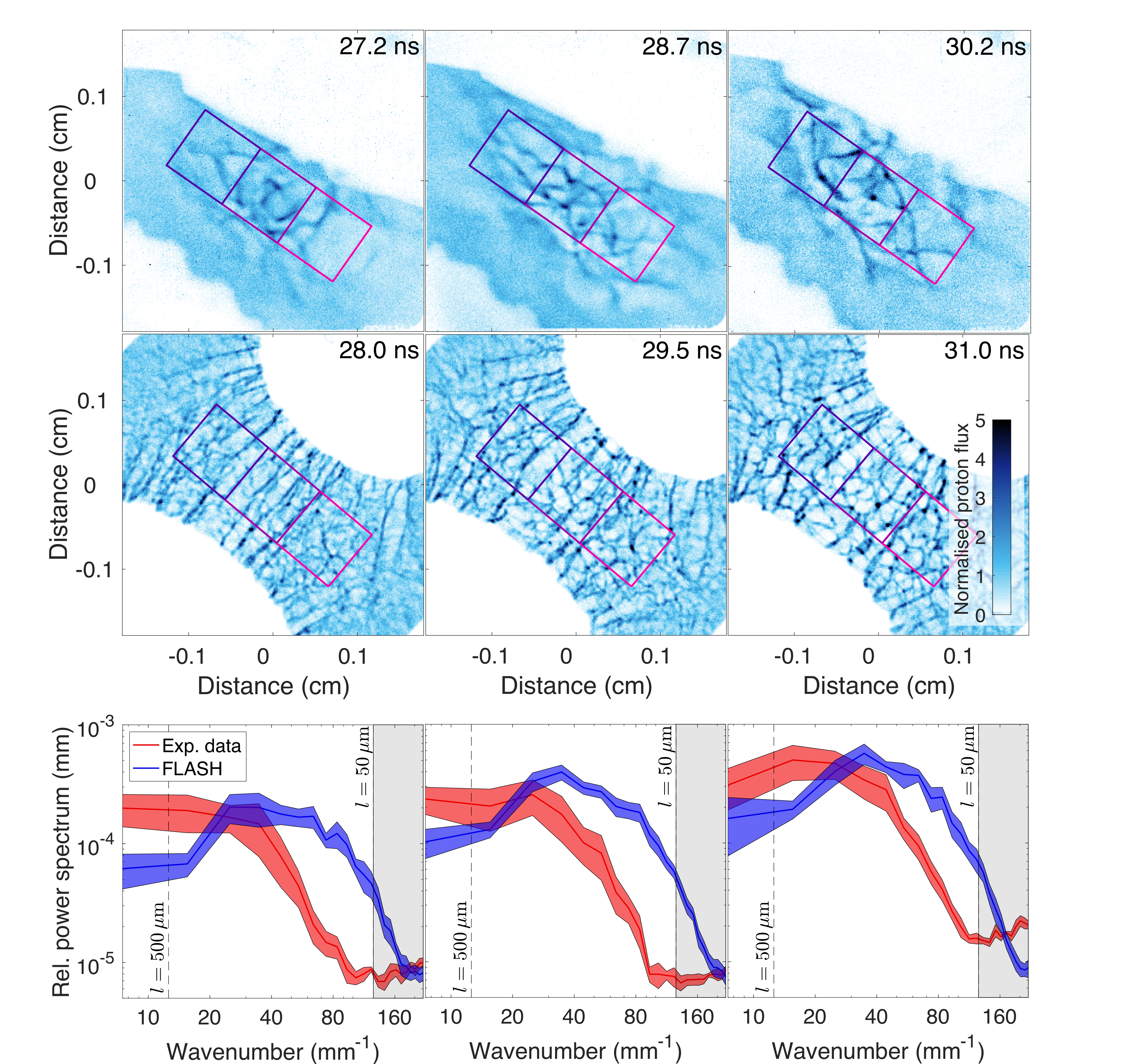
Figure 21: Investigating the characteristic scale of magnetic fluctuations by direct analysis of proton images. Top row: experimental proton images at specified times, along with an indication of regions to which spectral analysis is applied. Middle row: simulated 15.0 MeV FLASH proton images at specified times. The proton source and imaging set-up is modelled to be the same as the experiment’s; in particular, the source has a finite size of $50\,\mu$m. Bottom row: spectra of ‘relative’ (i.e., normalized to the mean) proton flux variations. The spectra in a given plot are calculated for the experimental and simulation data from the three regions depicted in the images directly above that plot. The uncertainty in the spectra is derived from the uncertainty in the spectra across the three regions.

References

- (1) P Arévalo, E Churazov, I Zhuravleva, C Hernández-Monteagudo, and M Revnivtsev, A Mexican hat with holes: calculating low-resolution power spectra from data with gaps. Monthly Notices of the Royal Astronomical Society 426, 1793 (2012)
- (2) J Colvin, and J Larsen, Extreme physics: properties and behaviour of matter at extreme conditions, (Cambridge University Press, Cambridge, 2014)
- (3) NL Kugland et al., Relation between electric and magnetic field structures and their proton-beam images, Review of Scientific Instruments 83, 101301 (2012)
- (4) DD Ryutov et al., Collisional effects in the ion Weibel instability for two counter-propagating plasma streams, Physics of Plasmas 21, 032701 (2014)
- (5) JD Huba, NRL plasma formulary. (Naval Research Laboratory, Washington DC, 1994)
- (6) CM Huntington et al., Observation of magnetic field generation via the Weibel instability in interpenetrating plasma flows, Nature Physics 11, 173 (2015)
- (7) AA Schekochihin, SC Cowley, SF Taylor, JL Maron, and JC McWilliams, Simulations of the small-scale turbulent dynamo, Astrophysics Journal 612, 276 (2004)
- (8) B. Fryxell et al., FLASH: An adaptive mesh hydrodynamics code for modeling astrophysical thermonuclear flashes, The Astrophysical Journal 131, 273 (2000)
- (9) P. Tzeferacos et al., FLASH MHD simulations of experiments that study shock-generated magnetic fields, High Energy Density Physics 17, 24 (2015)
- (10) M. Fatenejad et al., Collaborative comparison of simulation codes for high-energy-density physics applications, High Energy Density Physics 9, 63. (2013)
- (11) C. Orban et al., A radiation-hydrodynamics code comparison for laser-produced plasmas: FLASH versus HYDRA and the results of validation experiments, arXiv, 1306.1584 (2013)
- (12) J. Meinecke et al., Turbulent amplification of magnetic fields in laboratory laser-produced shock waves, Nature Physics 10, 520 (2014)
- (13) K. Falk et al., Equation of state measurements of warm dense carbon using laser-driven shock and release technique, Physical Review Letters 112, 155003 (2014)
- (14) R. Yurchak et al., Experimental demonstration of an inertial collimation mechanism in nested outflows, Physical Review Letters 112, 155001 (2014)
- (15) J. Meinecke et al., Developed turbulence and nonlinear amplification of magnetic fields in laboratory and astrophysical plasmas, Proceedings of the National Academy of Sciences 112, 8211 (2015)
- (16) C. Li et al., Scaled laboratory experiments explain the kink behaviour of the Crab Nebula jet, Nature Communications 7, 13081 (2016)
- (17) P. Tzeferacos et al., Numerical modeling of laser-driven experiments aiming to demonstrate magnetic field amplification via turbulent dynamo, Physics of Plasmas 24, 041404 (2017)
- (18) P. Tzeferacos et al., Laboratory evidence of dynamo amplification of magnetic fields in a turbulent plasma, Nature Communications 9, 591 (2018)
- (19) A. Rigby et al., Electron acceleration by wave turbulence in a magnetized plasma, Nature Physics 14, 475 (2018)
- (20) Y. Lu et al., Numerical simulation of magnetized jet creation using a hollow ring of laser beams, Physics of Plasmas 26 022902 (2019)
- (21) L. Gao et al., Mega-gauss plasma jet creation using a ring of laser beams, The Astrophysical Journal Letters, 873, L11 (2019)
- (22) T. G. White et al., Supersonic plasma turbulence in the laboratory, Nature Communications 10, 1758 (2019)
- (23) L. Chen et al., Transport of high-energy charged particles through spatially intermittent turbulent magnetic fields, The Astrophysical Journal 892, 114 (2020)
- (24) C. Li et al., Structure and dynamics of colliding plasma jets, Physical Review Letters 111, 235003 (2013)
- (25) J.S. Ross et al., Characterizing counter-streaming interpenetrating plasmas relevant to astrophysical collisionless shocks, Physics of Plasmas 19, 056501 (2012)
- (26) A. A. Schekochihin et al., Fluctuation dynamo and turbulent induction at low magnetic Prandtl numbers. New Journal of Physics 9, 300 (2007)
- (27) G. K. Batchelor Introduction to fluid dynamics, (Cambridge University Press, Cambridge, 1967)
- (28) F Rincon, Dynamo theories, Journal of Plasma Physics 85, 205850401 (2019)
- (29) A. Simionescu et al., Constraining gas motions in the intra-cluster medium. Space Sci Rev 215, 24 (2019)
- (30) I. Zhuravleva, E. Churazov, A. A. Schekochihin, S. W. Allen, A. Vikhlinin, and N. Werner, Suppressed effective viscosity in the bulk intergalactic plasma, Nature Astronomy 3, 832 (2019)
- (31) S. Chandrasekhar, The stability of superposed fluids: The Kelvin-Helmholtz instability, Hydrodynamic and Hydromagnetic Stability, chap. XI. (Oxford University Press, New York 1961)
- (32) T. Funada and D.‘D. Joseph, Viscous potential flow analysis of Kelvin–Helmholtz instability in a channel. Journal of Fluid Mechanics 445, 263 (2001)
- (33) A. Miura and P. L. Pritchett, Nonlocal stability analysis of the MHD Kelvin-Helmholtz instability in a compressible plasma. Journal of Geophysical Research 87, 7431 (1982)
- (34) AFA Bott, C Graziani, TG White, P Tzeferacos, DQ Lamb, G Gregori, and AA Schekochihin Proton imaging of stochastic magnetic fields, Journal of Plasma Physics 83, 6 (2017)