Social Optima in Leader-Follower Mean Field Linear Quadratic Control

Abstract.

This paper investigates a linear quadratic mean field leader-follower team problem, where the model involves one leader and a large number of weakly-coupled interactive followers. The leader and the followers cooperate to optimize the social cost. Specifically, for any strategy provided first by the leader, the followers would like to choose a strategy to minimize social cost functional. Using variational analysis and person-by-person optimality, we construct two auxiliary control problems. By solving sequentially the auxiliary control problems with consistent mean field approximations, we can obtain a set of decentralized social optimality strategy with help of a class of forward-backward consistency systems. The relevant Stackelberg equilibrium is further proved under some proper conditions.

Introduction

Mean field games have been studied by researchers from various aspects [7, 8, 10, 25]. They involve a large number of population and the interaction between each individual is negligible. The mean field game approach has been applied in many fields such as finance [14], economics [41], information technology [21], engineering [13, 24] and medicine [4]. The mean field linear quadratic (LQ) control problem is a special class of control problems, which can model many problems in applications and its solution exhibits elegant properties. For more work about the problem, readers can refer to [3, 9, 18, 19, 22, 26, 36, 37, 39, 44].

For the model with one major player and $N$ minor players, the state of the major player has a significant influence on state equations and cost functionals of other minor individuals, which can be considered as a strong effect of the major player on minor ones. Mean field games (control) with major and minor players have been discussed in some literature, such as [23, 32] for LQ problems, [6, 33] for nonlinear problems, [12, 20] for probabilistic approaches and [11] for finite-state problems. In such types of problem, there is no hierarchical structure of decision making between the major player and the minor players.

In contrast to the model discussed above, leader-follower (Stackelberg) problems contain at least two hierarchies of players. One hierarchy of the players is defined as the leaders with a major position and another hierarchy of the players is defined as the followers with a minor position. The leader has priority to announce a strategy first and then the followers seek their strategies to minimize their cost functionals with response to the given strategy of leader. According to the followers’ optimal points, the leader will choose his optimal strategy to minimize its cost functional. Leader-follower problem also has been widely investigated. For example, the two-person leader-follower problem combines with stochastic LQ differential game had been studied by Yong in [43] and the problem of one leader and $N$ followers who play a noncooperative game under LQ stochastic differential game had been studied by Moon and Basar in [31]. For further literature related to Stackelberg games, readers can refer to [1, 2, 27, 29, 34, 35, 38] .

Different from noncooperative games, the social optimization (team optimization) problem is a joint decision problem which all the players have the same goal and work cooperatively. The aim of each player is to select an optimal strategy and maximize the total payoff. Team optimization problem has been studied for many years. Marschak [30] first considered team optimization based on game theory. Ho and Chu studied team decision theory in optimal control problems [17]. Groves did the research of viewing the incentive problem as a team problem which the information for decisions is incomplete [16]. The team theory and person-by-person optimization with binary decision was investigated by Bauso and Pesenti [5] and the team problems under stochastic information structure with suboptimal solutions was studied in [15].

In this paper, we investigate social optimality of the leader-follower mean field LQ control problem. Our model contains one leader and $N$ followers. The leader’s state appears in both state equation and cost functional of each follower. It shows that the dynamics and cost functionals of the $N$ followers are directly influenced by the behavior of the leader. Unlike the model in [23, 31], our model has a population state average term in all state equations and cost functionals. This implies that such state dynamics and cost functionals are highly interactive and coupled. In reality, it is almost impossible for one player to obtain all the information of other players. Therefore, decentralized control which is based on the individual information set will be used instead of centralized control which is based on full information set and the information structure of each agent is different.

Compared with previous works, this paper mainly makes the following contributions:

• A social optimum problem is studied for mean field models with hierarchical structure. Unlike the problem in [31] where the leader and followers play a noncooperative game and try to minimize their own individual cost functional, all individuals in our models aim to minimize the social cost functional which equals the summation of cost functionals of all players. The $N$ followers are coupled by the population state average term. Since the cost functional presents individual performance in the game problems, the order of magnitude of the perturbation is $\frac{1}{N}$ which can be ignored. The population state average term may be approximated by a stochastic process directly (see [18]). However, in the team problems, the order of magnitude of the perturbation cannot be ignored after summing up all the cost functionals, which makes the problem very complicated. To overcome such difficulties, we approximate some terms as $N$ goes to infinity and use a duality procedure combined with auxiliary equations to transform the variation of the social cost functional into a standard LQ control form. Then, we construct an auxiliary control problem and a forward-backward consistency system which contains four equations to help us obtain the decentralized form of the optimal controls for the $N$ followers.

• The decentralized controls of the leader-follower problem are obtained and the solvability of a high-dimensional consistency condition system (CC system) is discussed. Since the leader’s state equation and cost functional are fully coupled with the followers’ state equations and cost functionals, it is more difficult to solve the leader’s problem. Except constructing auxiliary problem by mean field approximation as in the former part, we need to construct six auxiliary equations and use duality relations to obtain the decentralized form of the optimal control for the leader. Unlike the problem for $N$ followers, the final CC system of the leader’s problem contains ten equations which becomes a high-dimensional problem. To solve such equations directly is very difficult since they are fully coupled and have high-dimensional characteristics. We transform the high-dimensional CC system to a simple form of linear forward-backward stochastic differential equation (FBSDE; see [28, 42]) and discuss the solvability of the FBSDE through Ricatti equation method.

• The decentralized strategies of leader-follower problem are proved to be Stackelberg equilibrium by perturbation analysis. Different from [22, 23, 31, 40], we discuss the Stackelberg equilibrium for the team optimization problem. First, we need to prove the decentralized strategies for the followers have asymptotic social optimality. Because of the Stackelberg problem contains two hierarchies, we consider two coupled cost functionals (the leader and the followers) when using the standard method (see [22]). We prove the asymptotic optimality by decoupling them with two duality procedures and some arguments in error estimates. Second, we need to prove the decentralized strategies for the leader-follower problem is Stackelberg equilibrium. Also, some error estimates are very hard to be given directly since they are fully coupling. We decompose them by applying Ricatti equation method and then estimate them in proper order.

In the real world, our model can be used to describe some examples. For an automatic machine, the major part first gives an information to the system and the minor parts will adjust their parameters automatically such that the whole system keeps in the best state. For the economic environment, the small companies may hesitate to make decisions and often follow a monopoly company when facing to the volatility of the market. A monopoly company announces a decision first. Once the small companies try to make decisions according to their own situations, the monopoly company adjusts its decision such that the sum of the social wealth can be maximized. Moreover, the relationship between the employer and the employees or the federal government and the government in each state also can be described by our model.

The paper is organized as follows. The problem is formulated in Section 2. In Section 3, we solve the optimal controls for followers based on person-by-person optimality and obtain the CC system of the follower’s problem. In Section 4, we seek the social optimal solution of the leader’s problem and give the CC system of the leader’s problem. Then the CC system is transformed to a simple form of linear FBSDE in Section 5 and its wellposeness is discussed. In Section 6, we give the details of proving the Stackelberg equilibrium. Also, some prior lemmas will be introduced and proved. In Section 7, a numerical example is provided to simulate the efficiency of decentralized control. Section 8 is the conclusion of the paper.

Notation: Throughout this paper, $\mathbb{R}^{n\times m}$ and $\mathbb{S}^{n}$ denote the set of all $(n\times m)$ real matrices and the set of all $(n\times n)$ symmetric matrices, respectively. $\|\cdot\|$ is the standard Euclidean norm and $\langle\cdot,\cdot\rangle$ is the standard Euclidean inner product. For given symmetric matrix $S\geq 0$, the quadratic form $x^{T}Sx$ may be defined as $\|x\|_{S}^{2}$, where $x^{T}$ is the transpose of $x$. $C^{1}([0,T];\mathbb{R}^{n\times m})$ be the space of all $\mathbb{R}^{n\times m}$-valued continuously differentiable functions on $[0,T]$. For notation $o(1)$, $\lim_{n\rightarrow\infty}o(1)=0$. By [42], for sake of notation simplicity, we will use $K$ to denote a generic constant in following discussion. The value of $K$ may be different at different places and it only depends on the coefficients and initial values.

1. Problem formulation

Let $(\Omega,\mathcal{F},\mathbb{P})$ be a complete probability space which contains all $\mathbb{P}$-null sets in $\mathcal{F}$. $\xi_{i}\in\mathbb{R}^{n}$ are the values of the initial states and $W_{i}(\cdot)$ are $d$-dimensional standard Brownian motions, where $i=0,1,\cdots,N$. $\xi_{i}$ and $W_{i}(\cdot)$ are defined on $(\Omega,\mathcal{F},\mathbb{P})$. Consider a large-population system which contains one leader and $N$ followers. The state processes of the leader and the $i$th follower, $i=1,2,\cdots,N,$ are modeled by the following linear stochastic differential equations (SDE) on a finite time horizon $[0,T]$:

$$\left\{\begin{aligned} &dx_{0}(t)=[A_{0}(t)x_{0}(t)+B_{0}(t)u_{0}(t)+C_{0}(t)x^{(N)}(t)]dt+D_{0}(t)dW_{0}(t),\quad x_{0}(0)=\xi_{0},\\ &dx_{i}(t)=[A(t)x_{i}(t)+B(t)u_{i}(t)+C(t)x^{(N)}(t)+F(t)x_{0}(t)]dt+D(t)dW_{i}(t),\quad x_{i}(0)=\xi_{i},\\ \end{aligned}\right.$$ (1)

where $x^{(N)}(t):=\frac{1}{N}\sum_{i=1}^{N}x_{i}(t)$ is the state average of the followers. Let $\sigma$-algebra $\mathcal{F}_{t}^{i}=\sigma(W_{i}(s),0\leq s\leq t)$ and $\mathcal{G}_{t}^{i}=\mathcal{F}_{t}^{i}\bigvee\sigma\{\xi_{i},\xi_{0},W_{0}(s),0\leq s\leq t\}$, where $0\leq i\leq N$. $\mathcal{F}_{t}=\sigma(W_{i}(s),0\leq s\leq t,0\leq i\leq N)$ and $\mathcal{G}_{t}=\mathcal{F}_{t}\bigvee\sigma\{\xi_{i},0\leq i\leq N\}$. $\mathbb{F}^{i}=\{\mathcal{F}_{t}^{i}\}_{0\leq t\leq T}$ is the natural filtration generated by $W_{i}(\cdot)$ and $\mathbb{G}^{i}=\{\mathcal{G}_{t}^{i}\}_{0\leq t\leq T}$, where $0\leq i\leq N$. Correspondingly, we denote $\mathbb{F}=\{\mathcal{F}_{t}\}_{0\leq t\leq T}$, $\mathbb{G}=\{\mathcal{G}_{t}\}_{0\leq t\leq T}$. Next we introduce the following spaces:

$$L^{\infty}(0,T;\mathbb{R}^{n\times m})= \big{\{}\varphi:[0,T]\rightarrow\mathbb{R}^{n\times m}\big{|}\ \varphi(\cdot)\text{ is bounded and measurable}\big{\}},$$

$$L_{\mathbb{F}}^{2}(\Omega;\mathbb{R}^{m})= \big{\{}\xi:\Omega\rightarrow\mathbb{R}^{m}\big{|}\ \xi\text{ is }\mathbb{F}\text{-measurable, }\mathbb{E}\|\xi\|^{2}<\infty\big{\}},$$

$$L_{\mathbb{F}}^{2}(0,T;\mathbb{R}^{m})= \big{\{}x:[0,T]\times\Omega\rightarrow\mathbb{R}^{m}\big{|}\ x(\cdot)\text{ is }\mathbb{F}\text{-progressively}$$

$$\hskip 14.22636pt\text{measurable, }\|x(t)\|_{L^{2}}^{2}:=\mathbb{E}\int_{0}^{T}\|x(t)\|^{2}dt<\infty\big{\}},$$

$$L_{\mathbb{F}}^{2}(\Omega;C([0,T];\mathbb{R}^{m}))= \big{\{}x:[0,T]\times\Omega\rightarrow\mathbb{R}^{m}\big{|}\ x(\cdot)\text{ is }\mathbb{F}\text{-progressively}$$

$$\hskip 14.22636pt\text{measurable, continuous, }\mathbb{E}\sup_{t\in[0,T]}\|x(t)\|^{2}<\infty\big{\}},$$

$$\mathcal{M}[0,T]:=L_{\mathbb{F}}^{2}(\Omega; C([0,T];\mathbb{R}^{n}))\times L_{\mathbb{F}}^{2}(\Omega;C([0,T];\mathbb{R}^{m}))\times L_{\mathbb{F}}^{2}(0,T;\mathbb{R}^{m\times d}).$$

The set of admissible controls for the leader is defined as follows:

$$\mathcal{U}_{0}=\left\{u_{0}|u_{0}(t)\in L_{\mathbb{G}^{0}}^{2}(0,T;\mathbb{R}^{m})\right\},$$

and the set of admissible controls for the $i$th follower is defined as follows:

$$\mathcal{U}_{i}=\left\{u_{i}|u_{i}(t)\in L_{\mathbb{G}^{i}}^{2}(0,T;\mathbb{R}^{m})\right\},\quad 1\leq i\leq N.$$

These are the decentralized control sets and we let $\mathcal{U}=\mathcal{U}_{1}\times\mathcal{U}_{2}\times\cdots\times\mathcal{U}_{N}$. For comparison, the centralized control set is given by

$$\mathcal{U}_{c}=\Big{\{}(u_{0},u_{1},\cdots,u_{N})|u_{i}(t)\in L_{\mathbb{G}}^{2}(0,T;\mathbb{R}^{m}),0\leq i\leq N\Big{\}}.$$

Now we introduce the cost functionals of the leader and the $i$th follower, $1\leq i\leq N$. For the leader, the cost functional is defined as follows:

$$\mathcal{J}_{0}(u_{0}(\cdot);u(\cdot))= \mathbb{E}\bigg{\{}\int_{0}^{T}\big{[}\|x_{0}(t)-\Theta_{0}(t)x^{(N)}(t)-\eta_{0}(t)\|_{Q_{0}(t)}^{2}+\|u_{0}(t)\|_{R_{0}(t)}^{2}\big{]}dt$$ (2)

$$+\|x_{0}(T)-\hat{\Theta}_{0}x^{(N)}(T)-\hat{\eta}_{0}\|_{G_{0}}^{2}\bigg{\}},$$

where $u(\cdot)=(u_{1}(t),\cdots,u_{N}(t))\in\mathcal{U}_{c}$. $Q_{0}(\cdot)$, $R_{0}(\cdot)$ and $G_{0}(\cdot)$ are weight matrices. $Q_{0}(\cdot)$ and $\Theta_{0}(\cdot)$ represent the coupling between the leader and the population state average. This implies that the states of the followers can influence the cost functional of the leader. For the $i$th follower, the individual cost functional is defined as follows:

$$\mathcal{J}_{i}(u_{0}(\cdot);u(\cdot))= \mathbb{E}\bigg{\{}\int_{0}^{T}\big{[}\|x_{i}(t)-\Theta(t)x^{(N)}(t)-\Theta_{1}(t)x_{0}(t)-\eta(t)\|_{Q(t)}^{2}+\|u_{i}(t)\|_{R(t)}^{2}\big{]}dt$$ (3)

$$+\|x_{i}(T)-\hat{\Theta}x^{(N)}(T)-\hat{\Theta}_{1}x_{0}(T)-\hat{\eta}\|_{G}^{2}\bigg{\}},$$

where $Q(\cdot)$, $R(\cdot)$ and $G(\cdot)$ are weight matrices. $Q(\cdot)$, $\Theta(\cdot)$ and $\Theta_{1}(\cdot)$ represent the coupling between the $i$th follower, the population state average and the leader. This implies that the cost functional of the $i$th follower will be affected by the behavior of both the leader and the other followers. All the individuals in the system, including the leader and followers, aim to minimize the social cost functional, which is denoted by

$$\mathcal{J}_{soc}^{(N)}(u_{0}(\cdot);u(\cdot))=\alpha N\mathcal{J}_{0}(u_{0}(\cdot);u(\cdot))+\sum_{i=1}^{N}\mathcal{J}_{i}(u_{0}(\cdot);u(\cdot)),\quad\alpha>0.$$

Similar to [23] and [32], we have a scaling factor $\alpha N$ before $\mathcal{J}_{0}(u_{0}(\cdot);u(\cdot))$ such that $\mathcal{J}_{0}(u_{0}(\cdot);u(\cdot))$ and $\mathcal{J}_{i}(u_{0}(\cdot);u(\cdot))$ have the same order of magnitude. Otherwise, if $\alpha N=1$, then the performance of the leader will be insensitive when $N$ becomes larger. Now we introduce our assumptions.
(A1) The coefficients of (1), (2) and (3) satisfy

$$\left\{\begin{aligned} &A_{0}(\cdot),C_{0}(\cdot),A(\cdot),C(\cdot),F(\cdot)\in L^{\infty}(0,T;\mathbb{R}^{n\times n}),\\ &B_{0}(\cdot),B(\cdot)\in L^{\infty}(0,T;\mathbb{R}^{n\times m}),\quad D_{0}(\cdot),D(\cdot)\in L^{\infty}(0,T;\mathbb{R}^{n\times d}).\\ \end{aligned}\right.$$

$$\left\{\begin{aligned} &Q_{0}(\cdot),Q(\cdot)\in L^{\infty}(0,T;\mathbb{S}^{n}),\quad R_{0}(\cdot),R(\cdot)\in L^{\infty}(0,T;\mathbb{S}^{m}),\\ &\Theta_{0}(\cdot),\Theta_{1}(\cdot),\Theta(\cdot)\in L^{\infty}(0,T;\mathbb{R}^{n\times n}),\quad\eta_{0}(\cdot),\eta(\cdot)\in L^{2}(0,T;\mathbb{R}^{n}),\\ &\hat{\Theta}_{0},\hat{\Theta}_{1},\hat{\Theta}\in\mathbb{R}^{n\times n},\quad G_{0},G\in\mathbb{S}^{n},\quad\hat{\eta}_{0},\hat{\eta}\in\mathbb{R}^{n}.\end{aligned}\right.$$

(A2) $x_{0}(0)$ and $W_{0}(\cdot)$ are mutually independent. $\{x_{i}(0),1\leq i\leq N\}$ and $\{W_{i}(\cdot),1\leq i\leq N\}$ are independent of each other. $\mathbb{E}x_{i}(0)=\hat{\xi}$, $1\leq i\leq N$. For some constant $K$, which is independent of $N$, such that $\sup_{1\leq i\leq N}\mathbb{E}\|x_{i}(0)\|^{2}\leq K$. Furthermore, $x_{0}(0)$, $W_{0}(\cdot)$ and $\{x_{i}(0),1\leq i\leq N\}$, $\{W_{i}(t),1\leq i\leq N\}$ are independent of each other.
(A3) $Q_{0}(\cdot)\geq 0$, $R_{0}(\cdot)>\delta I$, $G_{0}\geq 0$ and $Q(\cdot)\geq 0$, $R(\cdot)>\delta I$, $G\geq 0$, for some $\delta>0$.

From now on, we may suppress the notation of time $t$ if necessary. We introduce our leader-follower problem: Under (A1)-(A3), for any $u_{0}\in\mathcal{U}_{0}$, to find a mapping $\mathcal{M}$: $\mathcal{U}_{0}\rightarrow\mathcal{U}$, and a control $\bar{u}_{0}\in\mathcal{U}_{0}$ such that

$$\left\{\begin{aligned} &\mathcal{J}_{soc}^{(N)}(u_{0};\mathcal{M}(u_{0}))=\inf_{u\in\mathcal{U}_{c}}\mathcal{J}_{soc}^{(N)}(u_{0};u),\\ &\mathcal{J}_{soc}^{(N)}(\bar{u}_{0};\mathcal{M}(\bar{u}_{0}))=\inf_{u_{0}\in\mathcal{U}_{0}}\mathcal{J}_{soc}^{(N)}(u_{0};\mathcal{M}(u_{0})).\end{aligned}\right.$$

Note that the $\mathcal{M}$ here is a mapping, which is different from the notation $\mathcal{M}[0,T]$ we just introduced.

2. The mean field LQ control problem for the $N$ followers

2.1. Person-by-person optimality

Fix $u_{0}\in\mathcal{U}_{0}$. The leader firstly announces his own open-loop strategy. Let $\bar{u}=\{\bar{u}_{1},\bar{u}_{2},\cdots,\bar{u}_{N}\}$ be the centralized optimal control of the followers and $\bar{x}=\{\bar{x}_{1},\bar{x}_{2},\cdots,\bar{x}_{N}\}$ be the corresponding states. Now we perturb $\bar{u}_{i}$ and fix other $\bar{u}_{j}$, where $j\neq i$. Then we denote $\delta u_{i}=u_{i}-\bar{u}_{i}$, $\delta x_{i}=x_{i}-\bar{x}_{i}$, where $u_{i}$ is the control after perturbing and $x_{i}$ is its corresponding state. The Fréchet differential $\delta\mathcal{J}_{0}(\delta u_{i})=\mathcal{J}_{0}(u_{0};u)-\mathcal{J}_{0}(u_{0};\bar{u})+o(\|\delta u_{i}\|)$ and $\delta\mathcal{J}_{i}(\delta u_{i})=\mathcal{J}_{i}(u_{0};u)-\mathcal{J}_{i}(u_{0};\bar{u})+o(\|\delta u_{i}\|)$, where $i=1,\cdots,N$. Therefore, the variations of the state equations for the leader, the $i$th follower and the $j$th follower, where $j\neq i$, are

$$\left\{\begin{aligned} &d\delta x_{0}=(A_{0}\delta x_{0}+C_{0}\delta x^{(N)})dt,\quad\delta x_{0}(0)=0,\\ &d\delta x_{i}=(A\delta x_{i}+B\delta u_{i}+C\delta x^{(N)}+F\delta x_{0})dt,\quad\delta x_{i}(0)=0,\\ &d\delta x_{j}=(A\delta x_{j}+C\delta x^{(N)}+F\delta x_{0})dt,\quad\delta x_{j}(0)=0,\quad j\neq i,\\ \end{aligned}\right.$$

and the variations of their corresponding cost functionals are

$$\frac{1}{2}\delta\mathcal{J}_{0}(\delta u_{i})= \mathbb{E}\bigg{\{}\int_{0}^{T}\langle Q_{0}(\bar{x}_{0}-\Theta_{0}\bar{x}^{(N)}-\eta_{0}),\delta x_{0}-\Theta_{0}\delta x^{(N)}\rangle dt$$

$$+\langle G_{0}(\bar{x}_{0}(T)-\hat{\Theta}_{0}\bar{x}^{(N)}(T)-\hat{\eta}_{0}),\delta x_{0}(T)-\hat{\Theta}_{0}\delta x^{(N)}(T)\rangle\bigg{\}},$$

$$\frac{1}{2}\delta\mathcal{J}_{i}(\delta u_{i})= \mathbb{E}\bigg{\{}\int_{0}^{T}\langle Q(\bar{x}_{i}-\Theta\bar{x}^{(N)}-\Theta_{1}\bar{x}_{0}-\eta),\delta x_{i}-\Theta\delta x^{(N)}-\Theta_{1}\delta x_{0}\rangle+\langle R\bar{u}_{i},\delta u_{i}\rangle dt$$

$$+\langle G(\bar{x}_{i}(T)-\hat{\Theta}\bar{x}^{(N)}(T)-\hat{\Theta}_{1}\bar{x}_{0}(T)-\hat{\eta}),\delta x_{i}(T)-\hat{\Theta}\delta x^{(N)}(T)-\hat{\Theta}_{1}\delta x_{0}(T)\rangle\bigg{\}},$$

$$\frac{1}{2}\delta\mathcal{J}_{j}(\delta u_{i})= \mathbb{E}\bigg{\{}\int_{0}^{T}\langle Q(\bar{x}_{j}-\Theta\bar{x}^{(N)}-\Theta_{1}\bar{x}_{0}-\eta),\delta x_{j}-\Theta\delta x^{(N)}-\Theta_{1}\delta x_{0}\rangle dt$$

$$+\langle G(\bar{x}_{j}(T)-\hat{\Theta}\bar{x}^{(N)}(T)-\hat{\Theta}_{1}\bar{x}_{0}(T)-\hat{\eta}),\delta x_{j}(T)-\hat{\Theta}\delta x^{(N)}(T)-\hat{\Theta}_{1}\delta x_{0}(T)\rangle\bigg{\}},$$

respectively. Consequently, we have the variation of the social cost functional as:

$$\frac{1}{2}\delta\mathcal{J}_{soc}^{(N)}(\delta u_{i})=\frac{1}{2}\bigg{[}\alpha N\delta\mathcal{J}_{0}(\delta u_{i})+\sum_{j\neq i}\delta\mathcal{J}_{j}(\delta u_{i})+\delta\mathcal{J}_{i}(\delta u_{i})\bigg{]}$$ (4)

$$=\mathbb{E}\bigg{\{}\int_{0}^{T}\alpha N\langle Q_{0}(\bar{x}_{0}-\Theta_{0}\bar{x}^{(N)}-\eta_{0}),\delta x_{0}\rangle-\alpha N\langle\Theta_{0}^{T}Q_{0}(\bar{x}_{0}-\Theta_{0}\bar{x}^{(N)}-\eta_{0}),\delta x^{(N)}\rangle+\langle Q(\bar{x}_{i}-\Theta\bar{x}^{(N)}$$

$$-\Theta_{1}\bar{x}_{0}-\eta),\delta x_{i}\rangle-\langle\Theta^{T}Q(\bar{x}_{i}-\Theta\bar{x}^{(N)}-\Theta_{1}\bar{x}_{0}-\eta),\delta x^{(N)}\rangle-\langle\Theta_{1}^{T}Q(\bar{x}_{i}-\Theta\bar{x}^{(N)}-\Theta_{1}\bar{x}_{0}-\eta),\delta x_{0}\rangle$$

$$+\langle R\bar{u}_{i},\delta u_{i}\rangle+\sum_{j\neq i}\langle Q(\bar{x}_{j}-\Theta\bar{x}^{(N)}-\Theta_{1}\bar{x}_{0}-\eta),\delta x_{j}\rangle-\sum_{j\neq i}\langle\Theta^{T}Q(\bar{x}_{j}-\Theta\bar{x}^{(N)}-\Theta_{1}\bar{x}_{0}-\eta),\delta x^{(N)}\rangle$$

$$-\sum_{j\neq i}\langle\Theta_{1}^{T}Q(\bar{x}_{j}-\Theta\bar{x}^{(N)}-\Theta_{1}\bar{x}_{0}-\eta),\delta x_{0}\rangle dt+\alpha N\langle G_{0}(\bar{x}_{0}(T)-\hat{\Theta}_{0}\bar{x}^{(N)}(T)-\hat{\eta}_{0}),\delta x_{0}(T)\rangle$$

$$-\alpha N\langle\hat{\Theta}_{0}^{T}G_{0}(\bar{x}_{0}(T)-\hat{\Theta}_{0}\bar{x}^{(N)}(T)-\hat{\eta}_{0}),\delta x^{(N)}(T)\rangle+\langle G(\bar{x}_{i}(T)-\hat{\Theta}\bar{x}^{(N)}(T)-\hat{\Theta}_{1}\bar{x}_{0}(T)-\hat{\eta}),\delta x_{i}(T)\rangle$$

$$-\langle\hat{\Theta}^{T}G(\bar{x}_{i}(T)-\hat{\Theta}\bar{x}^{(N)}(T)-\hat{\Theta}_{1}\bar{x}_{0}(T)-\hat{\eta}),\delta x^{(N)}(T)\rangle-\langle\hat{\Theta}_{1}^{T}G(\bar{x}_{i}(T)-\hat{\Theta}\bar{x}^{(N)}(T)-\hat{\Theta}_{1}\bar{x}_{0}(T)-\hat{\eta}),$$

$$\delta x_{0}(T)\rangle+\sum_{j\neq i}\langle G(\bar{x}_{j}(T)-\hat{\Theta}\bar{x}^{(N)}(T)-\hat{\Theta}_{1}\bar{x}_{0}(T)-\hat{\eta}),\delta x_{j}(T)\rangle-\sum_{j\neq i}\langle\hat{\Theta}^{T}G(\bar{x}_{j}(T)-\hat{\Theta}\bar{x}^{(N)}(T)-\hat{\Theta}_{1}\bar{x}_{0}(T)$$

$$-\hat{\eta}),\delta x^{(N)}(T)\rangle-\sum_{j\neq i}\langle\hat{\Theta}_{1}^{T}G(\bar{x}_{j}(T)-\hat{\Theta}\bar{x}^{(N)}(T)-\hat{\Theta}_{1}\bar{x}_{0}(T)-\hat{\eta}),\delta x_{0}(T)\rangle\bigg{\}}.$$

When $N\rightarrow\infty$, it follows that

$$\frac{1}{2}\delta\mathcal{J}_{soc}^{(N)}(\delta u_{i})=\mathbb{E}\bigg{\{}\int_{0}^{T}\alpha\langle Q_{0}(\bar{x}_{0}-\Theta_{0}\bar{x}^{(N)}-\eta_{0}),N\delta x_{0}\rangle-\alpha\langle\Theta_{0}^{T}Q_{0}(\bar{x}_{0}-\Theta_{0}\bar{x}^{(N)}-\eta_{0}),N\delta x^{(N)}\rangle$$

$$+\langle Q(\bar{x}_{i}-\Theta\bar{x}^{(N)}-\Theta_{1}\bar{x}_{0}-\eta),\delta x_{i}\rangle+\langle R\bar{u}_{i},\delta u_{i}\rangle+\langle\frac{1}{N}\sum_{j\neq i}Q(\bar{x}_{j}-\Theta\bar{x}^{(N)}-\Theta_{1}\bar{x}_{0}-\eta),N\delta x_{j}\rangle$$

$$-\langle\frac{1}{N}\sum_{j\neq i}\Theta^{T}Q(\bar{x}_{j}-\Theta\bar{x}^{(N)}-\Theta_{1}\bar{x}_{0}-\eta),N\delta x^{(N)}\rangle-\langle\frac{1}{N}\sum_{j\neq i}\Theta_{1}^{T}Q(\bar{x}_{j}-\Theta\bar{x}^{(N)}-\Theta_{1}\bar{x}_{0}-\eta),$$

$$N\delta x_{0}\rangle dt+\alpha\langle G_{0}(\bar{x}_{0}(T)-\hat{\Theta}_{0}\bar{x}^{(N)}(T)-\hat{\eta}_{0}),N\delta x_{0}(T)\rangle-\alpha\langle\hat{\Theta}_{0}^{T}G_{0}(\bar{x}_{0}(T)-\hat{\Theta}_{0}\bar{x}^{(N)}(T)-\hat{\eta}_{0}),$$

$$N\delta x^{(N)}(T)\rangle+\langle G(\bar{x}_{i}(T)-\hat{\Theta}\bar{x}^{(N)}(T)-\hat{\Theta}_{1}\bar{x}_{0}(T)-\hat{\eta}),\delta x_{i}(T)\rangle+\langle\frac{1}{N}\sum_{j\neq i}G(\bar{x}_{j}(T)-\hat{\Theta}\bar{x}^{(N)}(T)$$

$$-\hat{\Theta}_{1}\bar{x}_{0}(T)-\hat{\eta}),N\delta x_{j}(T)\rangle-\langle\frac{1}{N}\sum_{j\neq i}\hat{\Theta}^{T}G(\bar{x}_{j}(T)-\hat{\Theta}\bar{x}^{(N)}(T)-\hat{\Theta}_{1}\bar{x}_{0}(T)-\hat{\eta}),N\delta x^{(N)}(T)\rangle$$

$$-\langle\frac{1}{N}\sum_{j\neq i}\hat{\Theta}_{1}^{T}G(\bar{x}_{j}(T)-\hat{\Theta}\bar{x}^{(N)}(T)-\hat{\Theta}_{1}\bar{x}_{0}(T)-\hat{\eta}),N\delta x_{0}(T)\rangle\bigg{\}}+o(1).$$

Note that $\mathbb{E}\sup_{0\leq t\leq T}\|\delta x_{0}\|^{2}=O(\frac{1}{N^{2}})$, $\mathbb{E}\sup_{0\leq t\leq T}\|\delta x^{(N)}\|^{2}=O(\frac{1}{N^{2}})$ and $\langle\Theta^{T}Q(\bar{x}_{i}-\Theta\bar{x}^{(N)}-\Theta_{1}\bar{x}_{0}-\eta),\delta x^{(N)}\rangle+\langle\Theta_{1}^{T}Q(\bar{x}_{i}-\Theta\bar{x}^{(N)}-\Theta_{1}\bar{x}_{0}-\eta),\delta x_{0}\rangle+\langle\hat{\Theta}^{T}G(\bar{x}_{i}(T)-\hat{\Theta}\bar{x}^{(N)}(T)-\hat{\Theta}_{1}\bar{x}_{0}(T)-\hat{\eta}),\delta x^{(N)}(T)\rangle+\langle\hat{\Theta}_{1}^{T}G(\bar{x}_{i}(T)-\hat{\Theta}\bar{x}^{(N)}(T)-\hat{\Theta}_{1}\bar{x}_{0}(T)-\hat{\eta}),\delta x_{0}(T)\rangle=o(1)$ (the rigorous proof will be shown in Section 5). Let

$$\left\{\begin{aligned} &\delta x_{0}^{\dagger}=\lim_{N\rightarrow+\infty}(N\delta x_{0}),\\ &\delta x^{\dagger}=\lim_{N\rightarrow+\infty}(N\delta x_{j})=\lim_{N\rightarrow+\infty}(\sum_{j\neq i}\delta x_{j}),\ j\neq i.\end{aligned}\right.$$ (5)

Here $N\delta x_{0}$ converges to $\delta x_{0}^{\dagger}$ such that $\mathbb{E}\int_{0}^{T}\|N\delta x_{0}-\delta x_{0}^{\dagger}\|^{2}=O(\frac{1}{N^{2}})$. Similarly, $\sum_{j\neq i}\delta x_{j}$ and $N\delta x_{j}$ converge to $\delta x^{\dagger}$ (see Section 5 for the detailed proof). Then one can obtain

$$\left\{\begin{aligned} &d\delta x_{0}^{\dagger}=(A_{0}\delta x_{0}^{\dagger}+C_{0}\delta x_{i}+C_{0}\delta x^{\dagger})dt,\quad\quad\quad\delta x_{0}^{\dagger}(0)=0,\\ &d\delta x^{\dagger}=(A\delta x^{\dagger}+C\delta x_{i}+C\delta x^{\dagger}+F\delta x_{0}^{\dagger})dt,\quad\delta x^{\dagger}(0)=0.\\ \end{aligned}\right.$$ (6)

When $N\rightarrow\infty$, by mean field approximation, we use $\hat{x}$ to approximate $\bar{x}^{(N)}$. Note that $\hat{x}$ will be affected by $u_{0}$ which is given by the leader. Moreover, the influence of individual follower on $\hat{x}$ may be negligible. Hence, by straightforward computation, we simplified the social cost functional as follows:

$$\frac{1}{2}\delta\mathcal{J}_{soc}^{(N)}(\delta u_{i}) =\mathbb{E}\bigg{\{}\int_{0}^{T}\langle\alpha Q_{0}\Psi_{1}-\Theta_{1}^{T}Q\Psi_{3},\delta x_{0}^{\dagger}\rangle+\langle Q\Psi_{2}^{i}-\Theta^{T}Q\Psi_{3}-\alpha\Theta_{0}^{T}Q_{0}\Psi_{1},\delta x_{i}\rangle$$ (7)

$$+\langle R\bar{u}_{i},\delta u_{i}\rangle+\langle Q\Psi_{3}-\Theta^{T}Q\Psi_{3}-\alpha\Theta_{0}^{T}Q_{0}\Psi_{1},\delta x^{\dagger}\rangle dt+\langle\alpha G_{0}\Psi_{4}(T)$$

$$-\hat{\Theta}_{1}^{T}G\Psi_{6}(T),\delta x_{0}^{\dagger}(T)\rangle+\langle G\Psi_{6}(T)-\hat{\Theta}^{T}G\Psi_{6}(T)-\alpha\hat{\Theta}_{0}^{T}G_{0}\Psi_{4}(T),$$

$$\delta x^{\dagger}(T)\rangle+\langle G\Psi_{5}^{i}(T)-\hat{\Theta}^{T}G\Psi_{6}(T)-\alpha\hat{\Theta}_{0}^{T}G_{0}\Psi_{4}(T),\delta x_{i}(T)\rangle\bigg{\}},$$

where

$$\left\{\begin{aligned} &\Psi_{1}(\cdot):=\bar{x}_{0}-\Theta_{0}\hat{x}-\eta_{0},\quad\Psi_{2}^{i}(\cdot):=\bar{x}_{i}-\Theta\hat{x}-\Theta_{1}\bar{x}_{0}-\eta,\\ &\Psi_{3}(\cdot):=(I-\Theta)\hat{x}-\Theta_{1}\bar{x}_{0}-\eta,\\ \end{aligned}\right.$$

are related to time $t$, and

$$\left\{\begin{aligned} &\Psi_{4}(T):=\bar{x}_{0}(T)-\hat{\Theta}_{0}\hat{x}(T)-\hat{\eta}_{0},\quad\Psi_{5}^{i}(T):=\bar{x}_{i}(T)-\hat{\Theta}\hat{x}(T)-\hat{\Theta}_{1}\bar{x}_{0}(T)-\hat{\eta},\\ &\Psi_{6}(T):=(I-\hat{\Theta})\hat{x}(T)-\hat{\Theta}_{1}\bar{x}_{0}(T)-\hat{\eta},\\ \end{aligned}\right.$$

are related to time $T$ which are terminal terms.

It is very important to formulate an auxiliary control problem to obtain the decentralized optimal control for analyzing the problem of social optimality. Usually, an auxiliary control problem is a standard LQ control problem (see [22, 40]). However, (7) contains $\delta x_{0}^{\dagger}$ and $\delta x^{\dagger}$, which are the terms we do not want them appear in the social cost functional. Therefore, we need to use a duality procedure (see [44, Chapter 3]) to get off the dependence of $\delta\mathcal{J}_{soc}^{(N)}(\delta u_{i})$ on $\delta x_{0}^{\dagger}$ and $\delta x^{\dagger}$. To this end, we introduce two auxiliary equations

$$\left\{\begin{aligned} &dk_{1}=\alpha_{1}dt+\beta_{1}dW_{0},\ k_{1}(T)=\alpha G_{0}\Psi_{4}(T)-\hat{\Theta}_{1}^{T}G\Psi_{6}(T),\\ &dk_{2}=\alpha_{2}dt+\beta_{2}dW_{0},\ k_{2}(T)=(I-\hat{\Theta}^{T})G\Psi_{6}(T)-\alpha\hat{\Theta}_{0}^{T}G_{0}\Psi_{4}(T).\end{aligned}\right.$$ (8)

Using Itô formula, we have the following duality relations

$$\mathbb{E}\langle\alpha G_{0}\Psi_{4}(T)-\hat{\Theta}_{1}^{T}G\Psi_{6}(T),\delta x_{0}^{\dagger}(T)\rangle$$ (9)

$$=\mathbb{E}\langle k_{1}(0),\delta x_{0}^{\dagger}(0)\rangle+\mathbb{E}\int_{0}^{T}\langle k_{1},A_{0}\delta x_{0}^{\dagger}+C_{0}\delta x_{i}+C_{0}\delta x^{\dagger}\rangle+\langle\alpha_{1},\delta x_{0}^{\dagger}\rangle dt,$$

$$\mathbb{E}\langle(I-\hat{\Theta}^{T})G\Psi_{6}(T)-\alpha\hat{\Theta}_{0}^{T}G_{0}\Psi_{4}(T),\delta x^{\dagger}(T)\rangle$$

$$=\mathbb{E}\langle k_{2}(0),\delta x^{\dagger}(0)\rangle+\mathbb{E}\int_{0}^{T}\langle k_{2},A\delta x^{\dagger}+C\delta x_{i}+C\delta x^{\dagger}+F\delta x_{0}^{\dagger}\rangle+\langle\alpha_{2},\delta x^{\dagger}\rangle dt.$$

Putting (7) and (9) together, we obtain

$$\frac{1}{2}\delta\mathcal{J}_{soc}^{(N)}(\delta u_{i})= \mathbb{E}\bigg{\{}\int_{0}^{T}\langle R\bar{u}_{i},\delta u_{i}\rangle+\langle\alpha Q_{0}\Psi_{1}-\Theta_{1}^{T}Q\Psi_{3}+\alpha_{1}+F^{T}k_{2}+A_{0}^{T}k_{1},\delta x_{0}^{\dagger}\rangle$$

$$+\langle Q\Psi_{3}-\Theta^{T}Q\Psi_{3}-\alpha\Theta_{0}^{T}Q_{0}\Psi_{1}+C_{0}^{T}k_{1}+C^{T}k_{2}+\alpha_{2}+A^{T}k_{2},\delta x^{\dagger}\rangle$$

$$+\langle Q\Psi_{2}^{i}-\Theta^{T}Q\Psi_{3}-\alpha\Theta_{0}^{T}Q_{0}\Psi_{1}+C_{0}^{T}k_{1}+C^{T}k_{2},\delta x_{i}\rangle dt$$

$$+\langle G\Psi_{5}^{i}(T)-\hat{\Theta}^{T}G\Psi_{6}(T)-\alpha\hat{\Theta}_{0}^{T}G_{0}\Psi_{4}(T),\delta x_{i}(T)\rangle\bigg{\}}.$$

Comparing the coefficients, it follows that

$$\left\{\begin{aligned} &\alpha_{1}=-(\alpha Q_{0}\Psi_{1}-\Theta_{1}^{T}Q\Psi_{3}+F^{T}k_{2}+A_{0}^{T}k_{1}),\\ &\alpha_{2}=-(Q\Psi_{3}-\Theta^{T}Q\Psi_{3}-\alpha\Theta_{0}^{T}Q_{0}\Psi_{1}+C_{0}^{T}k_{1}+C^{T}k_{2}+A^{T}k_{2}).\end{aligned}\right.$$

Then, according to above discussion, the two auxiliary equations can be rewritten as:

$$\left\{\begin{aligned} &dk_{1}=-(\alpha Q_{0}\Psi_{1}-\Theta_{1}^{T}Q\Psi_{3}+F^{T}k_{2}+A_{0}^{T}k_{1})dt+\beta_{1}dW_{0},\\ &dk_{2}=-(Q\Psi_{3}-\Theta^{T}Q\Psi_{3}-\alpha\Theta_{0}^{T}Q_{0}\Psi_{1}+C_{0}^{T}k_{1}+C^{T}k_{2}+A^{T}k_{2})dt+\beta_{2}dW_{0},\\ &k_{1}(T)=\alpha G_{0}\Psi_{4}(T)-\hat{\Theta}_{1}^{T}G\Psi_{6}(T),\ k_{2}(T)=(I-\hat{\Theta}^{T})G\Psi_{6}(T)-\alpha\hat{\Theta}_{0}^{T}G_{0}\Psi_{4}(T),\end{aligned}\right.$$

and the variation of social cost functional is equivalent to

$$\frac{1}{2}\delta \mathcal{J}_{soc}^{(N)}(\delta u_{i})=\mathbb{E}\bigg{\{}\int_{0}^{T}\langle Q\bar{x}_{i},\delta x_{i}\rangle+\langle R\bar{u}_{i},\delta u_{i}\rangle+\langle-Q(\Theta\hat{x}+\Theta_{1}\bar{x}_{0}+\eta)$$ (10)

$$-\Theta^{T}Q\Psi_{3}-\alpha\Theta_{0}^{T}Q_{0}\Psi_{1}+C_{0}^{T}k_{1}+C^{T}k_{2},\delta x_{i}\rangle dt+\langle G\bar{x}_{i}(T),\delta x_{i}(T)\rangle$$

$$+\langle-G(\hat{\Theta}\hat{x}(T)+\hat{\Theta}_{1}\bar{x}_{0}(T)+\hat{\eta})-\hat{\Theta}^{T}G\Psi_{6}(T)-\alpha\hat{\Theta}_{0}^{T}G_{0}\Psi_{4}(T),\delta x_{i}(T)\rangle\bigg{\}}.$$

2.2. Decentralized strategy design for followers

As discussed in previous subsection, when $N$ is sufficiently large, a stochastic process $\hat{x}$ can be used to approximate $x^{(N)}$. Now, we can introduce the following auxiliary control problem for the $i$th follower. (P2) Minimize $\hat{\mathcal{J}_{i}}((u_{0},\hat{x});u_{i})$ over $u_{i}\in\mathcal{U}_{i}$, where

$$dx_{i}=[Ax_{i}+Bu_{i}+C\hat{x}+F\bar{x}_{0}(u_{0})]dt+DdW_{i},\ x_{i}(0)=\xi_{i},\ i=1,2,\cdots,N,\\$$ (11)

$$\hat{\mathcal{J}_{i}}((u_{0},\hat{x});u_{i})=\mathbb{E}\bigg{\{}\int_{0}^{T}\|x_{i}\|_{Q}^{2}+\|u_{i}\|_{R}^{2}+2\langle\chi_{1},x_{i}\rangle dt+\|x_{i}(T)\|_{G}^{2}+2\langle\chi_{2},x_{i}(T)\rangle\bigg{\}},$$ (12)

with

$$\left\{\begin{aligned} &\chi_{1}=-Q(\Theta\hat{x}+\Theta_{1}\bar{x}_{0}(u_{0})+\eta)-\Theta^{T}Q\Psi_{3}-\alpha\Theta_{0}^{T}Q_{0}\Psi_{1}+C_{0}^{T}k_{1}+C^{T}k_{2},\\ &\chi_{2}=-G(\hat{\Theta}\hat{x}(T)+\hat{\Theta}_{1}\bar{x}_{0}(u_{0})(T)+\hat{\eta})-\hat{\Theta}^{T}G\Psi_{6}(T)-\alpha\hat{\Theta}_{0}^{T}G_{0}\Psi_{4}(T).\end{aligned}\right.$$

Here, $\bar{x}_{0}(u_{0})$ means $\bar{x}_{0}$ is related to $u_{0}$. $\bar{x}_{0}$, $\hat{x}$, $k_{1}$ and $k_{2}$ are determined by

$$\left\{\begin{aligned} &d\bar{x}_{0}=[A_{0}\bar{x}_{0}+B_{0}u_{0}+C_{0}\hat{x}]dt+D_{0}dW_{0},\quad\bar{x}_{0}(0)=\xi_{0},\\ &d\hat{x}=[A\hat{x}+B\hat{u}+C\hat{x}+F\bar{x}_{0}(u_{0})]dt,\quad\hat{x}(0)=\hat{\xi},\\ &dk_{1}=-(\alpha Q_{0}\Psi_{1}-\Theta_{1}^{T}Q\Psi_{3}+F^{T}k_{2}+A_{0}^{T}k_{1})dt+\beta_{1}dW_{0},\\ &dk_{2}=-(Q\Psi_{3}-\Theta^{T}Q\Psi_{3}-\alpha\Theta_{0}^{T}Q_{0}\Psi_{1}+C_{0}^{T}k_{1}+C^{T}k_{2}+A^{T}k_{2})dt+\beta_{2}dW_{0},\\ &k_{1}(T)=\alpha G_{0}\Psi_{4}(T)-\hat{\Theta}_{1}^{T}G\Psi_{6}(T),\ k_{2}(T)=(I-\hat{\Theta}^{T})G\Psi_{6}(T)-\alpha\hat{\Theta}_{0}^{T}G_{0}\Psi_{4}(T),\end{aligned}\right.$$ (13)

where $\hat{x}$ and $\hat{u}$ are the approximations of $x^{(N)}$ and $\frac{1}{N}\sum_{i=1}^{N}u_{i}$, respectively.

In what follows, we let $\bar{u}=\mathcal{M}(u_{0})=\{\bar{u}_{1},\bar{u}_{2},\cdots,\bar{u}_{N}\}\in\mathcal{U}$. Note that $\bar{u}$ here represents the decentraliezd optimal control, which is different from the same notation in the beginning of Section 2. Assume that (A1)-(A3) hold. For given $u_{0}\in\mathcal{U}_{0}$, (P2) has a unique optimal control

$$\bar{u}_{i}=-R^{-1}B^{T}p_{i},$$

where $p_{i}$ is an adaptive solution to the following backward stochastic differential equation (BSDE)

$$dp_{i}=-(A^{T}p_{i}+Q\bar{x}_{i}+\chi_{1})dt+\zeta_{0}dW_{0}+\zeta_{i}dW_{i},\ p_{i}(T)=G\bar{x_{i}}(T)+\chi_{2}.$$

Proof.

The variation of the state equation in (11) is

$$d\delta x_{i}=(A\delta x_{i}+B\delta u_{i})dt,\ \delta x_{i}(0)=0,\quad i=1,2,\cdots,N,$$

and the variation of the corresponding cost functional is

$$\frac{1}{2}\delta\hat{\mathcal{J}_{i}}((u_{0},\hat{x});u_{i})=\mathbb{E}\bigg{\{}\int_{0}^{T}\langle Q\bar{x}_{i},\delta x_{i}\rangle+\langle R\bar{u}_{i},\delta u_{i}\rangle+\langle\chi_{1},\delta x_{i}\rangle dt+\langle G\bar{x}_{i}(T),\delta x_{i}(T)\rangle+\langle\chi_{2},\delta x_{i}(T)\rangle\bigg{\}}.$$ (14)

Using a similar argument from (8) to (10), we construct the following auxiliary equation

$$dp_{i}=\theta_{i}dt+\zeta_{0}dW_{0}+\zeta_{i}dW_{i},\ p_{i}(T)=G\bar{x}_{i}(T)+\chi_{2},$$ (15)

and have the following duality relation between $p_{i}$ and $\delta x_{i}$ by using Itô formula

$$\mathbb{E}\langle p_{i}(T),\delta x_{i}(T)\rangle= \mathbb{E}\langle p_{i}(0),\delta x_{i}(0)\rangle+\mathbb{E}\int_{0}^{T}\langle A^{T}p_{i}+\theta_{i},\delta x_{i}\rangle+\langle B^{T}p_{i},\delta u_{i}\rangle dt.$$

For given $u_{0}\in\mathcal{U}_{0}$, since $Q\geq 0$ and $R>\delta I$, for some $\delta>0$, (12) is uniformly convex and it has a unique optimal control. Let (14) equal zero, we have

$$\theta_{i}=-(A^{T}p_{i}+Q\bar{x}_{i}+\chi_{1}),\quad\bar{u}_{i}=-R^{-1}B^{T}p_{i}.$$ (16)

Then, the proposition follows. ∎

Substituting (16) into (11) and (15), we have the following FBSDE

$$\left\{\begin{aligned} &d\bar{x}_{i}=[A\bar{x}_{i}-BR^{-1}B^{T}p_{i}+C\hat{x}+F\bar{x}_{0}]dt+DdW_{i},\ x_{i}(0)=\xi_{i},\ i=1,2,\cdots,N,\\ &dp_{i}=-(A^{T}p_{i}+Q\bar{x}_{i}+\chi_{1})dt+\zeta_{0}dW_{0}+\zeta_{i}dW_{i},\ p_{i}(T)=Gx_{i}(T)+\chi_{2}.\end{aligned}\right.$$ (17)

By taking limits, the above FBSDE can be rewritten as:

$$\left\{\begin{aligned} &d\hat{x}=[(A+C)\hat{x}+F\bar{x}_{0}-BR^{-1}B^{T}\hat{p}]dt,\ \hat{x}(0)=\hat{\xi},\\ &d\hat{p}=-(A^{T}\hat{p}+Q\hat{x}+\chi_{1})dt+\zeta_{0}dW_{0},\ \hat{p}(T)=G\hat{x}(T)+\chi_{2}.\end{aligned}\right.$$ (18)

2.3. The consistency condition of the follower problem

Let

$$\left\{\begin{aligned} &\Xi_{1}:=(I-\Theta^{T})Q(I-\Theta)+\alpha\Theta_{0}^{T}Q_{0}\Theta_{0},\ \Xi_{1}^{G}:=(I-\hat{\Theta}^{T})G(I-\hat{\Theta})+\alpha\hat{\Theta}_{0}^{T}G_{0}\hat{\Theta}_{0},\\ &\Xi_{2}:=(I-\Theta^{T})Q\Theta_{1}+\alpha\Theta_{0}^{T}Q_{0},\ \Xi_{2}^{G}:=(I-\hat{\Theta}^{T})G\hat{\Theta}_{1}+\alpha\hat{\Theta}_{0}^{T}G_{0},\\ &\Xi_{3}:=(I-\Theta^{T})Q\eta-\alpha\Theta_{0}^{T}Q_{0}\eta_{0},\ \Xi_{3}^{G}:=(I-\hat{\Theta}^{T})G\hat{\eta}-\alpha\hat{\Theta}_{0}^{T}G_{0}\hat{\eta}_{0},\\ &\Xi_{4}:=\Theta_{1}^{T}Q\Theta_{1}+\alpha Q_{0},\ \Xi_{4}^{G}:=\hat{\Theta}_{1}^{T}G\hat{\Theta}_{1}+\alpha G_{0},\\ &\Xi_{5}:=\Theta_{1}^{T}Q\eta-\alpha Q_{0}\eta_{0},\ \Xi_{5}^{G}:=\hat{\Theta}_{1}^{T}G\hat{\eta}-\alpha G_{0}\hat{\eta}_{0}.\end{aligned}\right.$$

Combining (13) and (18), we can obtain the CC system

$$\left\{\begin{aligned} &d\hat{x}=[(A+C)\hat{x}+F\bar{x}_{0}-BR^{-1}B^{T}k_{2}]dt,\ \hat{x}(0)=\hat{\xi},\\ &d\bar{x}_{0}=[A_{0}\bar{x}_{0}+B_{0}u_{0}+C_{0}\hat{x}]dt+D_{0}dW_{0},\ \bar{x}_{0}(0)=\xi_{0},\\ &dk_{1}=-[\Xi_{4}\bar{x}_{0}-\Xi_{2}^{T}\hat{x}+A_{0}^{T}k_{1}+F^{T}k_{2}+\Xi_{5}]dt+\beta_{1}dW_{0},\\ &dk_{2}=-[\Xi_{1}\hat{x}-\Xi_{2}\bar{x}_{0}+C_{0}^{T}k_{1}+(A+C)^{T}k_{2}-\Xi_{3}]dt+\beta_{2}dW_{0},\\ &k_{1}(T)=\Xi_{4}^{G}\bar{x}_{0}(T)-(\Xi_{2}^{G})^{T}\hat{x}(T)+\Xi_{5}^{G},\ k_{2}(T)=\Xi_{1}^{G}\hat{x}(T)-\Xi_{2}^{G}\bar{x}_{0}(T)-\Xi_{3}^{G},\end{aligned}\right.$$ (19)

where $\hat{p}=k_{2}$ can be easily verified.

3. The optimal control problem for the leader

Now, let (P2) have a unique solution. Then, for $u_{0}\in\mathcal{U}_{0}$ given by leader, the followers choose their optimal control $\bar{u}=\mathcal{M}(u_{0})=\{\bar{u}_{1},\bar{u}_{2},\cdots,\bar{u}_{N}\}\in\mathcal{U}$, where $\bar{u}_{i}$ is shown in (16). Now we consider the optimal control of the leader to further minimize the social cost functional. In the infinite population system, $x^{(N)}$ may be approximated by $\hat{x}$. Hence, we can construct the following auxiliary optimal control problem for the leader. (P3) Minimize $\hat{\mathcal{J}}_{soc}^{(N)}(u_{0};\bar{u})$ over $u_{0}\in\mathcal{U}_{0}$, where

$$dx_{0}=[A_{0}x_{0}+B_{0}u_{0}+C_{0}\hat{x}]dt+D_{0}dW_{0},\quad x_{0}(0)=\xi_{0},$$ (20)

$$\hat{\mathcal{J}}_{soc}^{(N)}(u_{0};\bar{u})=\alpha N\hat{\mathcal{J}}_{0}(u_{0};\bar{u})+\sum_{i=1}^{N}\hat{\mathcal{J}}_{i}(u_{0};\bar{u}).$$

(P3) is based on (P2). Therefore, combining (16), the equations below (7) and the equations (2), (3) with mean field approximations, the cost functionals of the leader and the $i$th follower are

$$\hat{\mathcal{J}}_{0}(u_{0};\bar{u})= \mathbb{E}\bigg{\{}\int_{0}^{T}\langle Q_{0}\Psi_{1},\Psi_{1}\rangle+\langle R_{0}u_{0},u_{0}\rangle dt+\langle G_{0}\Psi_{4},\Psi_{4}\rangle\bigg{\}},$$

$$\hat{\mathcal{J}}_{i}(u_{0};\bar{u})= \mathbb{E}\bigg{\{}\int_{0}^{T}\langle Q\Psi_{2}^{i},\Psi_{2}^{i}\rangle+\langle B^{T}p_{i},R^{-1}B^{T}p_{i}\rangle dt+\langle G\Psi_{5}^{i},\Psi_{5}^{i}\rangle\bigg{\}},$$

where $\hat{x}$, $\bar{x}_{0}$, $k_{1}$, $k_{2}$, $\bar{x}_{i}$, $p_{i}$ are determined by (19) and (17). Using a similar argument in Section 2, we let $\bar{u}_{0}$ be the optimal strategy of the leader and perturb $u_{0}$ in (20), where $\delta u_{0}=u_{0}-\bar{u}_{0}$. Since $\bar{x}_{0}$, $\hat{x}$, $\bar{x}_{i}$ and $p_{i}$ are determined by $u_{0}$, we denote their corresponding perturbations as: $\delta\bar{x}_{0}=\bar{x}_{0}(u_{0})-\bar{x}_{0}(\bar{u}_{0})$, $\delta\hat{x}=\hat{x}(u_{0})-\hat{x}(\bar{u}_{0})$, $\delta\bar{x}_{i}=\bar{x}_{i}(u_{0})-\bar{x}_{i}(\bar{u}_{0})$ and $\delta p_{i}=p_{i}(u_{0})-p_{i}(\bar{u}_{0})$. For sake of notation simplicity, we drop $(\bar{u}_{0})$ in the following $\bar{x}_{0}(\bar{u}_{0})$, $\hat{x}(\bar{u}_{0})$, $\bar{x}_{i}(\bar{u}_{0})$ and $p_{i}(\bar{u}_{0})$, etc. Then, one can obtain

$$d\delta\bar{x}_{0}=[A_{0}\delta\bar{x}_{0}+B_{0}\delta u_{0}+C_{0}\delta\hat{x}]dt,\ \delta\bar{x}_{0}(0)=0,$$

and the variations of corresponding cost functionals

$$\frac{1}{2}\delta\hat{\mathcal{J}}_{0}(\delta u_{0})= \mathbb{E}\bigg{\{}\int_{0}^{T}\langle Q_{0}\Psi_{1},\delta\bar{x}_{0}-\Theta_{0}\delta\hat{x}\rangle+\langle R_{0}\bar{u}_{0},\delta u_{0}\rangle dt+\langle G_{0}\Psi_{4},\delta\bar{x}_{0}(T)-\hat{\Theta}_{0}\delta\hat{x}(T)\rangle\bigg{\}},$$

$$\frac{1}{2}\sum_{i=1}^{N}\delta\hat{\mathcal{J}}_{i}(\delta u_{0})=\sum_{i=1}^{N}\mathbb{E}\bigg{\{}\int_{0}^{T}\langle Q\Psi_{2}^{i},\delta\bar{x}_{i}-\Theta\delta\hat{x}-\Theta_{1}\delta\bar{x}_{0}\rangle+\langle R^{-1}B^{T}p_{i},B^{T}\delta p_{i}\rangle dt$$

$$\hskip 28.45274pt+\langle G\Psi_{5}^{i},\delta\bar{x}_{i}(T)-\hat{\Theta}\delta\hat{x}(T)-\hat{\Theta}_{1}\delta\bar{x}_{0}(T)\rangle\bigg{\}}.$$

Here $\Psi_{1}$, $\Psi_{2}^{i}$, $\Psi_{4}(T)$, $\Psi_{5}^{i}(T)$, are related to $\bar{u}_{0}$. In what follows, $\Psi_{1}$, $\Psi_{2}^{i}$, $\Psi_{3}$, $\Psi_{4}(T)$, $\Psi_{5}^{i}(T)$, $\Psi_{6}(T)$ will be related to $\bar{u}_{0}$. Therefore, the variation of the social cost functional is

$$\frac{1}{2}\delta\hat{\mathcal{J}}_{soc}^{(N)}(\delta u_{0})$$ (21)

$$= \alpha N\mathbb{E}\int_{0}^{T}\langle Q_{0}\Psi_{1},\delta\bar{x}_{0}\rangle-\langle\Theta_{0}^{T}Q_{0}\Psi_{1},\delta\hat{x}\rangle+\langle R_{0}\bar{u}_{0},\delta u_{0}\rangle dt$$

$$+\sum_{i=1}^{N}\mathbb{E}\int_{0}^{T}\langle Q\Psi_{2}^{i},\delta\bar{x}_{i}\rangle-\langle\Theta^{T}Q\Psi_{2}^{i},\delta\hat{x}\rangle-\langle\Theta_{1}^{T}Q\Psi_{2}^{i},\delta\bar{x}_{0}\rangle+\langle BR^{-1}B^{T}p_{i},\delta p_{i}\rangle dt$$

$$+\alpha N\langle G_{0}\Psi_{4}(T),\delta\bar{x}_{0}(T)\rangle-\alpha N\langle\hat{\Theta}_{0}^{T}G_{0}\Psi_{4}(T),\delta\hat{x}(T)\rangle-\sum_{i=1}^{N}\langle\hat{\Theta}_{1}^{T}G\Psi_{5}^{i}(T),\delta\bar{x}_{0}(T)\rangle$$

$$-\sum_{i=1}^{N}\langle\hat{\Theta}^{T}G\Psi_{5}^{i}(T),\delta\hat{x}(T)\rangle+\sum_{i=1}^{N}\langle G\Psi_{5}^{i}(T),\delta\bar{x}_{i}(T)\rangle.$$

Similarly, the variations of those equations in (17) and (19) are given by

$$\left\{\begin{aligned} &d\delta\bar{x}_{i}=[A\delta\bar{x}_{i}-BR^{-1}B^{T}\delta p_{i}+C\delta\hat{x}+F\delta\bar{x}_{0}]dt,\quad\delta\bar{x}_{i}(0)=0,\quad i=1,2,\cdots,N,\\ &d\delta p_{i}=-(A^{T}\delta p_{i}+Q\delta x_{i}+[\Xi_{1}-Q]\delta\hat{x}-\Xi_{2}\delta\bar{x}_{0}+C_{0}^{T}\delta k_{1}+C^{T}\delta k_{2})dt+\delta\zeta_{0}dW_{0}+\delta\zeta_{i}dW_{i},\\ &\delta p_{i}(T)=G\delta x_{i}(T)+[\Xi_{1}^{G}-G]\delta\hat{x}(T)-\Xi_{2}^{G}\delta\bar{x}_{0}(T),\end{aligned}\right.$$

and

$$\left\{\begin{aligned} &d\delta\hat{x}=[(A+C)\delta\hat{x}+F\delta\bar{x}_{0}-BR^{-1}B^{T}\delta k_{2}]dt,\quad\delta\hat{x}(0)=0,\\ &d\delta k_{1}=-[\Xi_{4}\delta\bar{x}_{0}-\Xi_{2}^{T}\delta\hat{x}+A_{0}^{T}\delta k_{1}+F^{T}\delta k_{2}]dt+\delta\beta_{1}dW_{0},\\ &d\delta k_{2}=-[\Xi_{1}\delta\hat{x}-\Xi_{2}\delta\bar{x}_{0}+C_{0}^{T}\delta k_{1}+(A+C)^{T}\delta k_{2}]dt+\delta\beta_{2}dW_{0},\\ &\delta k_{1}(T)=\Xi_{4}^{G}\delta\bar{x}_{0}(T)-(\Xi_{2}^{G})^{T}\delta\hat{x}(T),\quad\delta k_{2}(T)=\Xi_{1}^{G}\delta\hat{x}(T)-\Xi_{2}^{G}\delta\bar{x}_{0}(T).\\ \end{aligned}\right.$$

Since (21) contains many terms that we do not want them appear in the social cost functional, we will use a similar argument in Section 2 to get off the dependence of $\delta\hat{\mathcal{J}}_{soc}^{(N)}(\delta u_{0})$ on those terms. Therefore, we need to construct six auxiliary equations to help us obtain the optimal control of the leader. We introduce the first three auxiliary equations:

$$\left\{\begin{aligned} &dq_{i}=m_{i}dt+n_{i}^{0}dW_{0}+n_{i}dW_{i},\quad q_{i}(0)=0,\quad i=1,2,\cdots,N,\\ &dl_{1}=s_{1}dt+r_{1}dW_{0},\quad l_{1}(0)=0,\\ &dl_{2}=s_{2}dt+r_{2}dW_{0},\quad l_{2}(0)=0.\end{aligned}\right.$$

Here $q_{i}$, $l_{1}$ and $l_{2}$ are used to free $\delta\hat{\mathcal{J}}_{soc}^{(N)}(\delta u_{0})$ from the dependence on $p_{i}$, $k_{1}$ and $k_{2}$, respectively. By a similar argument from (8) to (10), we can rewrite the variation of the social cost functional as follows:

$$\frac{1}{2}\delta\hat{\mathcal{J}}_{soc}^{(N)}(\delta u_{0})$$

$$=\mathbb{E}\int_{0}^{T}\sum_{i=1}^{N}\langle\alpha Q_{0}\Psi_{1}-\Theta_{1}^{T}Q\Psi_{2}^{i},\delta\bar{x}_{0}\rangle+\sum_{i=1}^{N}\langle-\alpha\Theta_{0}^{T}Q_{0}\Psi_{1}-\Theta^{T}Q\Psi_{2}^{i},\delta\hat{x}\rangle+\sum_{i=1}^{N}\langle Q\Psi_{2}^{i},\delta\bar{x}_{i}\rangle$$

$$+N\langle\alpha R_{0}\bar{u}_{0},\delta u_{0}\rangle+\sum_{i=1}^{N}\langle BR^{-1}B^{T}p_{i},\delta p_{i}\rangle+\sum_{i=1}^{N}\langle l_{1},-(A_{0}^{T}\delta k_{1}+F^{T}\delta k_{2}+\Xi_{4}\delta\bar{x}_{0}-\Xi_{2}^{T}\delta\hat{x})\rangle$$

$$+\sum_{i=1}^{N}\langle s_{1},\delta k_{1}\rangle+\sum_{i=1}^{N}\langle s_{2},\delta k_{2}\rangle+\sum_{i=1}^{N}\langle l_{2},-((A+C)^{T}\delta k_{2}+C_{0}^{T}\delta k_{1}+\Xi_{1}\delta\hat{x}-\Xi_{2}\delta\bar{x}_{0})\rangle$$

$$+\sum_{i=1}^{N}\langle-(A^{T}\delta p_{i}+Q\delta\bar{x}_{i}+[\Xi_{1}-Q]\delta\hat{x}-\Xi_{2}\delta\bar{x}_{0}+C_{0}^{T}\delta k_{1}+C^{T}\delta k_{2}),q_{i}\rangle+\sum_{i=1}^{N}\langle\delta p_{i},m_{i}\rangle$$

$$+\sum_{i=1}^{N}[\langle\delta\beta_{1},r_{1}\rangle+\langle\delta\beta_{2},r_{2}\rangle]+\sum_{i=1}^{N}[\langle\delta\zeta_{0},n_{i}^{0}\rangle+\langle\delta\zeta_{i},n_{i}\rangle]dt+\sum_{i=1}^{N}\langle G\Psi_{5}^{i}(T)-Gq_{i}(T),\delta\bar{x}_{i}(T)\rangle$$

$$+\sum_{i=1}^{N}\langle\alpha G_{0}\Psi_{4}(T)-\hat{\Theta}_{1}^{T}G\Psi_{5}^{i}(T)-(\Xi_{4}^{G})^{T}l_{1}(T)+(\Xi_{2}^{G})^{T}l_{2}(T)+(\Xi_{2}^{G})^{T}q_{i}(T),\delta\bar{x}_{0}(T)\rangle$$

$$-\sum_{i=1}^{N}\langle\alpha\hat{\Theta}_{0}^{T}G_{0}\Psi_{4}(T)+\hat{\Theta}^{T}G\Psi_{5}^{i}(T)-(\Xi_{2}^{G})^{T}l_{1}(T)+(\Xi_{1}^{G})^{T}l_{2}(T)+(\Xi_{1}^{G}-G)^{T}q_{i}(T),\delta\hat{x}(T)\rangle.$$

Next, we introduce another three auxiliary equations:

$$\left\{\begin{aligned} &d\hat{y}^{i}=\hat{\alpha}dt+\hat{\beta}dW_{0}+\sum_{i=1}^{N}\hat{\beta}_{i}dW_{i},\\ &\hat{y}^{i}(T)=\alpha\hat{\Theta}_{0}^{T}G_{0}\Psi_{4}(T)+\hat{\Theta}^{T}G\Psi_{5}^{i}(T)-(\Xi_{2}^{G})^{T}l_{1}(T)+(\Xi_{1}^{G})^{T}l_{2}(T)+(\Xi_{1}^{G}-G)^{T}q_{i}(T),\\ &dy_{0}^{i}=\hat{\alpha}_{0}dt+\hat{\beta}_{0}dW_{0}+\sum_{i=1}^{N}\hat{\beta}_{i}^{0}dW_{i},\\ &y_{0}^{i}(T)=\alpha G_{0}\Psi_{4}(T)-\hat{\Theta}_{1}^{T}G\Psi_{5}^{i}(T)-(\Xi_{4}^{G})^{T}l_{1}(T)+(\Xi_{2}^{G})^{T}l_{2}(T)+(\Xi_{2}^{G})^{T}q_{i}(T),\\ &dy_{i}=\alpha_{i}dt+\beta_{0}dW_{0}+\beta_{i}dW_{i},\quad y_{i}(T)=G\Psi_{5}^{i}(T)-Gq_{i}(T),\quad i=1,2,\cdots,N.\end{aligned}\right.$$

Here $\hat{y}^{i}$, $y_{0}^{i}$ and $y_{i}$ are used to free $\delta\hat{\mathcal{J}}_{soc}^{(N)}(\delta u_{0})$ from the dependence on $\delta\hat{x}$, $\delta\bar{x}_{0}$ and $\delta\bar{x}_{i}$, respectively. Similarly, by Itô formula and the duality relations, the variation of the social cost functional can be further rewritten as follows:

$$\frac{1}{2}\delta\hat{\mathcal{J}}_{soc}^{(N)}(\delta u_{0})$$

$$= \mathbb{E}\int_{0}^{T}\sum_{i=1}^{N}\langle\alpha Q_{0}\Psi_{1}-\Theta_{1}^{T}Q\Psi_{2}^{i}+F^{T}y_{i}-F^{T}\hat{y}^{i}+A_{0}^{T}y_{0}^{i}+\hat{\alpha}_{0}-\Xi_{4}^{T}l_{1}+\Xi_{2}^{T}l_{2}$$

$$+\Xi_{2}^{T}q_{i},\delta\bar{x}_{0}\rangle+\sum_{i=1}^{N}\langle-\alpha\Theta_{0}^{T}Q_{0}\Psi_{1}-\Theta^{T}Q\Psi_{2}^{i}+C^{T}y_{i}-(A+C)^{T}\hat{y}^{i}+C_{0}^{T}y_{0}^{i}$$

$$-\hat{\alpha}+\Xi_{2}l_{1}-\Xi_{1}^{T}l_{2}-(\Xi_{1}-Q)^{T}q_{i},\delta\hat{x}\rangle+\sum_{i=1}^{N}\langle Q\Psi_{2}^{i}+A^{T}y_{i}+\alpha_{i}-Qq_{i},\delta\bar{x}_{i}\rangle$$

$$+\sum_{i=1}^{N}\langle BR^{-1}B^{T}p_{i}-BR^{-1}B^{T}y_{i}+m_{i}-Aq_{i},\delta p_{i}\rangle+\sum_{i=1}^{N}[\langle n_{i},\delta\zeta_{i}\rangle+\langle n_{i}^{0},\delta\zeta_{0}\rangle]$$

$$+\sum_{i=1}^{N}\langle s_{1}-C_{0}l_{2}-A_{0}l_{1}+C_{0}q_{i},\delta k_{1}\rangle+\sum_{i=1}^{N}\langle s_{2}-(A+C)l_{2}+BR^{-1}B^{T}\hat{y}^{i}-Fl_{1}$$

$$+Cq_{i},\delta k_{2}\rangle+\sum_{i=1}^{N}[\langle r_{1},\delta\beta_{1}\rangle+\langle r_{2},\delta\beta_{2}\rangle]+\langle\alpha NR_{0}\bar{u}_{0}+\sum_{i=1}^{N}B_{0}^{T}y_{0}^{i},\delta u_{0}\rangle dt.$$

Using a similar discussion in Proposition 2.1 and comparing the coeffcients, we have

$$\left\{\begin{aligned} &\hat{\alpha}_{0}=-(\alpha Q_{0}\Psi_{1}-\Theta_{1}^{T}Q\Psi_{2}^{i}+F^{T}y_{i}-F^{T}\hat{y}^{i}+A_{0}^{T}y_{0}^{i}-\Xi_{4}^{T}l_{1}+\Xi_{2}^{T}l_{2}+\Xi_{2}^{T}q_{i}),\\ &\hat{\alpha}=-\alpha\Theta_{0}^{T}Q_{0}\Psi_{1}-\Theta^{T}Q\Psi_{2}^{i}+C^{T}y_{i}-(A+C)^{T}\hat{y}^{i}+C_{0}^{T}y_{0}^{i}+\Xi_{2}l_{1}-\Xi_{1}^{T}l_{2}-(\Xi_{1}-Q)^{T}q_{i},\\ &\alpha_{i}=-(Q\Psi_{2}^{i}+A^{T}y_{i}-Q^{T}q_{i}),\quad m_{i}=-(BR^{-1}B^{T}p_{i}-BR^{-1}B^{T}y_{i}-Aq_{i}),\\ &s_{1}=C_{0}l_{2}+A_{0}l_{1}-C_{0}q_{i},\quad s_{2}=(A+C)l_{2}-BR^{-1}B^{T}\hat{y}^{i}+Fl_{1}-Cq_{i},\\ &n_{i}=0,\quad n_{i}^{0}=0,\quad r_{1}=0,\quad r_{2}=0.\\ \end{aligned}\right.$$

Then, we have following FBSDE

$$\left\{\begin{aligned} &dy_{i}=-(A^{T}y_{i}-Q^{T}q_{i}+Q\Psi_{2}^{i})dt+\beta_{0}dW_{0}+\beta_{i}dW_{i},\quad y_{i}(T)=G\Psi_{5}^{i}(T)-Gq_{i}(T),\\ &dq_{i}=(BR^{-1}B^{T}y_{i}+Aq_{i}-BR^{-1}B^{T}p_{i})dt,\quad q_{i}(0)=0,\quad i=1,2,\cdots,N,\\ &d\hat{y}^{i}=(-\alpha\Theta_{0}^{T}Q_{0}\Psi_{1}-\Theta^{T}Q\Psi_{2}^{i}+C^{T}y_{i}-(A+C)^{T}\hat{y}^{i}+C_{0}^{T}y_{0}^{i}+\Xi_{2}l_{1}-\Xi_{1}^{T}l_{2}\\ &\hskip 22.76228pt-(\Xi_{1}-Q)^{T}q_{i})dt+\hat{\beta}dW_{0}+\sum_{i=1}^{N}\hat{\beta}_{i}dW_{i},\\ &\hat{y}^{i}(T)=\alpha\hat{\Theta}_{0}^{T}G_{0}\Psi_{4}(T)+\hat{\Theta}^{T}G\Psi_{5}^{i}(T)-(\Xi_{2}^{G})^{T}l_{1}(T)+(\Xi_{1}^{G})^{T}l_{2}(T)+(\Xi_{1}^{G}-G)^{T}q_{i}(T),\\ &dy_{0}^{i}=-(\alpha Q_{0}\Psi_{1}-\Theta_{1}^{T}Q\Psi_{2}^{i}+F^{T}y_{i}-F^{T}\hat{y}^{i}+A_{0}^{T}y_{0}^{i}-\Xi_{4}^{T}l_{1}+\Xi_{2}^{T}l_{2}+\Xi_{2}^{T}q_{i})dt\\ &\hskip 28.45274pt+\hat{\beta}_{0}dW_{0}+\sum_{i=1}^{N}\hat{\beta}_{i}^{0}dW_{i},\\ &y_{0}^{i}(T)=\alpha G_{0}\Psi_{4}(T)-\hat{\Theta}_{1}^{T}G\Psi_{5}^{i}(T)-(\Xi_{4}^{G})^{T}l_{1}(T)+(\Xi_{2}^{G})^{T}l_{2}(T)+(\Xi_{2}^{G})^{T}q_{i}(T),\\ &dl_{1}=(A_{0}l_{1}+C_{0}l_{2}-C_{0}q_{i})dt,\quad l_{1}(0)=0,\\ &dl_{2}=[Fl_{1}+(A+C)l_{2}-BR^{-1}B^{T}\hat{y}^{i}-Cq_{i}]dt,\quad l_{2}(0)=0,\end{aligned}\right.$$ (22)

with the centralized form of the optimal control for the leader

$$\bar{u}_{0}=-\frac{\alpha^{-1}}{N}R_{0}^{-1}B_{0}^{T}\sum_{i=1}^{N}y_{0}^{i}:=u_{0}^{(N)}.$$ (23)

Note that $\bar{u}_{0}$ relies on $N$. Denote

$$\left\{\begin{aligned} &y^{*}=\lim_{N\rightarrow+\infty}\frac{1}{N}\sum_{i=1}^{N}y_{i},\quad\hat{y}^{*}=\lim_{N\rightarrow+\infty}\frac{1}{N}\sum_{i=1}^{N}\hat{y}^{i},\quad y_{0}^{*}=\lim_{N\rightarrow+\infty}\frac{1}{N}\sum_{i=1}^{N}y_{0}^{i},\\ &q^{*}=\lim_{N\rightarrow+\infty}\frac{1}{N}\sum_{i=1}^{N}q_{i},\quad l_{1}^{*}=\lim_{N\rightarrow+\infty}\frac{1}{N}\sum_{i=1}^{N}l_{1},\quad l_{2}^{*}=\lim_{N\rightarrow+\infty}\frac{1}{N}\sum_{i=1}^{N}l_{2}.\end{aligned}\right.$$

Here, using a similar argument of (5), we can easily prove that $\frac{1}{N}\sum_{i=1}^{N}y_{i}$, $\frac{1}{N}\sum_{i=1}^{N}\hat{y}^{i}$, $\frac{1}{N}\sum_{i=1}^{N}y_{0}^{i}$, $\frac{1}{N}\sum_{i=1}^{N}q_{i}$, $\frac{1}{N}\sum_{i=1}^{N}l_{1}$ and $\frac{1}{N}\sum_{i=1}^{N}l_{2}$ converge to $y^{*}$, $\hat{y}^{*}$, $y_{0}^{*}$, $q^{*}$, $l_{1}^{*}$ and $l_{2}^{*}$, respectively. Thus, combining (19) and (22), when $N\rightarrow\infty$, we can obtain the CC system for the leader-follower problem

$$\left\{\begin{aligned} &d\hat{x}=[(A+C)\hat{x}+F\bar{x}_{0}-BR^{-1}B^{T}k_{2}]dt,\quad\hat{x}(0)=\hat{\xi},\\ &d\bar{x}_{0}=[A_{0}\bar{x}_{0}+C_{0}\hat{x}-B_{0}(\alpha R_{0})^{-1}B_{0}^{T}y_{0}^{*}]dt+D_{0}dW_{0},\quad\bar{x}_{0}(0)=\xi_{0},\\ &dk_{1}=-[\Xi_{4}\bar{x}_{0}-\Xi_{2}^{T}\hat{x}+A_{0}^{T}k_{1}+F^{T}k_{2}+\Xi_{5}]dt+\beta_{1}dW_{0},\\ &dk_{2}=-[\Xi_{1}\hat{x}-\Xi_{2}\bar{x}_{0}+C_{0}^{T}k_{1}+(A+C)^{T}k_{2}-\Xi_{3}]dt+\beta_{2}dW_{0},\\ &k_{1}(T)=\Xi_{4}^{G}\bar{x}_{0}(T)-(\Xi_{2}^{G})^{T}\hat{x}(T)+\Xi_{5}^{G},\quad k_{2}(T)=\Xi_{1}^{G}\hat{x}(T)-\Xi_{2}^{G}\bar{x}_{0}(T)-\Xi_{3}^{G},\\ &dy^{*}=-(A^{T}y^{*}-Q^{T}q^{*}+Q\Psi_{3})dt+\beta^{*}dW_{0},\quad y^{*}(T)=G\Psi_{6}(T)-Gq^{*}(T),\\ &dq^{*}=(BR^{-1}B^{T}y^{*}+Aq^{*}-BR^{-1}B^{T}k_{2})dt,\quad q^{*}(0)=0,\\ &d\hat{y}^{*}=[-\alpha\Theta_{0}^{T}Q_{0}\Psi_{1}-\Theta^{T}Q\Psi_{3}+C^{T}y^{*}-(A+C)^{T}\hat{y}^{*}+C_{0}^{T}y_{0}^{*}+\Xi_{2}l_{1}^{*}-\Xi_{1}^{T}l_{2}^{*}\\ &\hskip 22.76228pt-(\Xi_{1}-Q)^{T}q^{*}]dt+\hat{\beta}^{*}dW_{0},\\ &\hat{y}^{*}(T)=\alpha\hat{\Theta}_{0}^{T}G_{0}\Psi_{4}(T)+\hat{\Theta}^{T}G\Psi_{6}(T)-(\Xi_{2}^{G})^{T}l_{1}^{*}(T)+(\Xi_{1}^{G})^{T}l_{2}^{*}(T)+(\Xi_{1}^{G}-G)^{T}q^{*}(T),\\ &dy_{0}^{*}=-(\alpha Q_{0}\Psi_{1}-\Theta_{1}^{T}Q\Psi_{3}+F^{T}y^{*}-F^{T}\hat{y}^{*}+A_{0}^{T}y_{0}^{*}-\Xi_{4}^{T}l_{1}^{*}+\Xi_{2}^{T}l_{2}^{*}+\Xi_{2}^{T}q^{*})dt\\ &\hskip 28.45274pt+\hat{\beta}_{0}^{*}dW_{0},\\ &y_{0}^{*}(T)=\alpha G_{0}\Psi_{4}(T)-\hat{\Theta}_{1}^{T}G\Psi_{6}(T)-(\Xi_{4}^{G})^{T}l_{1}^{*}(T)+(\Xi_{2}^{G})^{T}l_{2}^{*}(T)+(\Xi_{2}^{G})^{T}q^{*}(T),\\ &dl_{1}^{*}=(A_{0}l_{1}^{*}+C_{0}l_{2}^{*}-C_{0}q^{*})dt,\quad l_{1}^{*}(0)=0,\\ &dl_{2}^{*}=[Fl_{1}^{*}+(A+C)l_{2}^{*}-BR^{-1}B^{T}\hat{y}^{*}-Cq^{*}]dt,\quad l_{2}^{*}(0)=0.\end{aligned}\right.$$ (24)

and the decentralized optimal control for the leader

$$u_{0}^{*}=-(\alpha R_{0})^{-1}B_{0}^{T}y_{0}^{*}.$$ (25)

The final CC system is highly coupled with five forward equations and five backward equations. The existence and uniqueness of (24) is very important for obtaining the optimal control, however it is very difficult to solve such high-dimensional system. We need to simplify the CC system to a FBSDE using block matrices and these will be discussed in next section.

4. Well-posedness of the CC system

Note that in (24), the equations of $(\hat{x},\bar{x}_{0},k_{1},k_{2})$ form a coupled FBSDE and $(y^{*},q^{*},\hat{y}^{*},y_{0}^{*},l_{1}^{*},l_{2}^{*})$ form another coupled FBSDE. The two FBSDEs are also fully coupled with each other. Therefore, we try to look at the above FBSDEs in a different way. To this end, we set

Then (24) is equivalent to

$$\left\{\begin{aligned} &d\mathbb{X}=[\mathbb{A}\mathbb{X}+\mathbb{B}\mathbb{Y}+b]dt+\mathbb{D}dW_{0},\quad\mathbb{X}(0)=(\hat{\xi}^{T}\quad\xi_{0}^{T}\quad 0\quad 0\quad 0)^{T},\\ &d\mathbb{Y}=[\hat{\mathbb{A}}\mathbb{X}+\hat{\mathbb{B}}\mathbb{Y}+\hat{b}]dt+\hat{\mathbb{D}}dW_{0},\quad\mathbb{Y}(T)=\mathbb{G}\mathbb{X}(T)+g,\end{aligned}\right.$$ (26)

with

$$b=\left(\begin{array}[]{c}0\\ 0\\ 0\\ 0\\ 0\\ \end{array}\right),\quad\mathbb{D}=\left(\begin{array}[]{c}0\\ D_{0}\\ 0\\ 0\\ 0\\ \end{array}\right),\quad\hat{\mathbb{A}}=\left(\begin{array}[]{ccccc}-Q(I-\Theta)&Q\Theta_{1}&Q^{T}&0&0\\ \Xi_{1}-Q(I-\Theta)&-\Xi_{2}+Q\Theta_{1}&-(\Xi_{1}-Q)^{T}&\Xi_{2}&-\Xi_{1}^{T}\\ \Xi_{2}^{T}&-\Xi_{4}&-\Xi_{2}^{T}&\Xi_{4}^{T}&-\Xi_{2}^{T}\\ \Xi_{2}^{T}&-\Xi_{4}&0&0&0\\ -\Xi_{1}&\Xi_{2}&0&0&0\\ \end{array}\right),$$

$$\hat{b}=\left(\begin{array}[]{c}Q\eta\\ -\Xi_{3}+Q\eta\\ -\Xi_{5}\\ -\Xi_{5}\\ \Xi_{3}\\ \end{array}\right),\quad\hat{\mathbb{D}}=\left(\begin{array}[]{c}\beta^{*}\\ \hat{\beta}^{*}\\ \hat{\beta}_{0}^{*}\\ \beta_{1}\\ \beta_{2}\\ \end{array}\right),\quad\hat{\mathbb{B}}=\left(\begin{array}[]{ccccc}-A^{T}&0&0&0&0\\ C^{T}&-(A+C)^{T}&C_{0}^{T}&0&0\\ -F^{T}&F^{T}&-A_{0}^{T}&0&0\\ 0&0&0&-A_{0}^{T}&-F^{T}\\ 0&0&0&-C_{0}^{T}&-(A+C)^{T}\\ \end{array}\right),$$

$$g=\left(\begin{array}[]{c}-G\hat{\eta}\\ \Xi_{3}^{G}-G\hat{\eta}\\ \Xi_{5}^{G}\\ \Xi_{5}^{G}\\ -\Xi_{3}^{G}\\ \end{array}\right),\quad\mathbb{G}=\left(\begin{array}[]{ccccc}G(I-\hat{\Theta})&-G\hat{\Theta}_{1}&-G&0&0\\ -\Xi_{1}^{G}+G(I-\hat{\Theta})&\Xi_{2}^{G}-G\hat{\Theta}_{1}&(\Xi_{1}^{G}-G)^{T}&-(\Xi_{2}^{G})^{T}&(\Xi_{1}^{G})^{T}\\ -(\Xi_{2}^{G})^{T}&\Xi_{4}^{G}&(\Xi_{2}^{G})^{T}&-(\Xi_{4}^{G})^{T}&(\Xi_{2}^{G})^{T}\\ -(\Xi_{2}^{G})^{T}&\Xi_{4}^{G}&0&0&0\\ \Xi_{1}^{G}&-\Xi_{2}^{G}&0&0&0\\ \end{array}\right).$$

Denote

$$\bar{\mathbb{A}}=\left(\begin{array}[]{cc}\mathbb{A}+\mathbb{B}\mathbb{G}&\mathbb{B}\\ \hat{\mathbb{A}}-\mathbb{G}\mathbb{A}+\hat{\mathbb{B}}\mathbb{G}-\mathbb{G}\hat{\mathbb{B}}\mathbb{G}&\hat{\mathbb{B}}-\mathbb{G}\mathbb{B}\\ \end{array}\right),\quad\bar{b}=\left(\begin{array}[]{c}b\\ \hat{b}-\mathbb{G}b\\ \end{array}\right),\quad\bar{\mathbb{D}}=\left(\begin{array}[]{c}\mathbb{D}\\ \hat{\mathbb{D}}\\ \end{array}\right),\quad\bar{\mathbb{Y}}=\mathbb{Y}-\mathbb{G}\mathbb{X}.$$

Then (26) can be rewritten as:

$$\left\{\begin{aligned} &d\left(\begin{array}[]{c}\mathbb{X}\\ \bar{\mathbb{Y}}\\ \end{array}\right)=\left\{\bar{\mathbb{A}}\left(\begin{array}[]{c}\mathbb{X}\\ \bar{\mathbb{Y}}\\ \end{array}\right)+\bar{b}\right\}dt+\bar{\mathbb{D}}dW_{0},\\ &\mathbb{X}(0)=(\hat{\xi}^{T}\quad\xi_{0}^{T}\quad 0\quad 0\quad 0)^{T},\quad\bar{\mathbb{Y}}(T)=g.\end{aligned}\right.$$ (27)

This is a fully coupled FBSDE. From the Theorem 3.7 of Chapter 2 in [28], the FBSDE (27) is solvable for all $g\in L_{\mathbb{F}}^{2}(\Omega;\mathbb{R}^{5n})$ if and only if the following condition holds:

$$\det\left\{(0,I)e^{\bar{\mathbb{A}}t}\left(\begin{array}[]{c}0\\ I\end{array}\right)\right\}>0,\quad\forall\ t\in[0,T].$$ (28)

In the case, (26) admits an unique solution for any given $g\in L_{\mathbb{F}}^{2}(\Omega;\mathbb{R}^{5n})$.

Under the condition (28), we may decouple the FBSDE (27) by

$$\bar{\mathbb{Y}}=\mathbb{K}\mathbb{X}+\kappa,\quad\ t\in[0,T],$$

where $\mathbb{K}\in C^{1}([0,T];\mathbb{S}^{5n})$ is a solution of the following Ricatti equation

$$\dot{\mathbb{K}}+\mathbb{K}(\mathbb{A}+\mathbb{B}\mathbb{G})+\mathbb{K}\mathbb{B}\mathbb{K}-(\hat{\mathbb{B}}-\mathbb{G}\mathbb{B})\mathbb{K}-(\hat{\mathbb{A}}-\mathbb{G}\mathbb{A}+\hat{\mathbb{B}}\mathbb{G}-\mathbb{G}\hat{\mathbb{B}}\mathbb{G})=0,\ t\in[0,T],\quad\mathbb{K}(T)=0,$$

and $\kappa\in C^{1}([0,T];\mathbb{R}^{5n})$ satisfies

$$\dot{\kappa}+(\mathbb{K}\mathbb{B}-(\hat{\mathbb{B}}-\mathbb{G}\mathbb{B}))\kappa+\mathbb{K}b-(\hat{b}-\mathbb{G}b)=0,\ t\in[0,T],\quad\kappa(T)=g.$$ (29)

By the Theorem 3.7 and Theorem 4.3 of Chapter 2 in [28], if (28) hold, then the Ricatti equation admits a unique solution $\mathbb{K}(\cdot)$ which has the following representation:

$$\mathbb{K}=-\bigg{[}(0,I)e^{\bar{\mathbb{A}}(T-t)}\left(\begin{array}[]{c}0\\ I\end{array}\right)\bigg{]}^{-1}\bigg{[}(0,I)e^{\bar{\mathbb{A}}(T-t)}\left(\begin{array}[]{c}I\\ 0\end{array}\right)\bigg{]},\quad t\in[0,T].$$ (30)

Consider the system (27) with parameters $A_{0}=0.1$, $B_{0}=1$, $C_{0}=0.01$, $D_{0}=1$, $A=0.05$, $B=1$, $C=0.05$, $D=1$, $F=0.3$, $\Theta_{0}=1$, $Q_{0}=1$, $R_{0}=10$, $G_{0}=0$, $\Theta=0.1$, $\Theta_{1}=1$, $Q=0.9$, $R=15$, $G=0$, $\alpha=1.02$, $T=12$, $\eta_{0}=\eta=0$. Then, we have

$$\mathbb{A}=\small{\left(\begin{array}[]{ccccc}0.10&0.30&0&0&0\\ 0.01&0.10&0&0&0\\ 0&0&0.05&0&0\\ 0&0&-0.01&0.10&0.01\\ 0&0&-0.05&0.30&0.10\\ \end{array}\right)},\mathbb{B}=\small{\left(\begin{array}[]{ccccc}0&0&0&0&-0.0667\\ 0&0&-0.0980&0&0\\ 0.0667&0&0&0&-0.0667\\ 0&0&0&0&0\\ 0&-0.0667&0&0&0\\ \end{array}\right)},$$

$$\hat{\mathbb{A}}=\small{\left(\begin{array}[]{ccccc}-0.81&0.90&0.90&0&0\\ 0.939&-0.93&-2.649&1.83&-1.749\\ 1.83&-1.92&-1.83&1.92&-1.83\\ 1.83&-1.92&0&0&0\\ -1.749&1.83&0&0&0\\ \end{array}\right)},\hat{\mathbb{B}}=\small{\left(\begin{array}[]{ccccc}-0.05&0&0&0&0\\ 0.05&-0.10&0.01&0&0\\ -0.30&0.30&-0.10&0&0\\ 0&0&0&-0.10&-0.30\\ 0&0&0&-0.01&-0.10\\ \end{array}\right)}.$$

Hence, according to the simulation through Matlab software, for any $t\in[0,T]$, we obtain

$$\bar{\mathbb{A}}=\left(\begin{array}[]{cc}\mathbb{A}+\mathbb{B}\mathbb{G}&\mathbb{B}\\ \hat{\mathbb{A}}-\mathbb{G}\mathbb{A}+\hat{\mathbb{B}}\mathbb{G}-\mathbb{G}\hat{\mathbb{B}}\mathbb{G}&\hat{\mathbb{B}}-\mathbb{G}\mathbb{B}\\ \end{array}\right),\quad\quad\det\left\{(0,I)e^{\bar{\mathbb{A}}t}\left(\begin{array}[]{c}0\\ I\end{array}\right)\right\}>0,$$

(e.g. for $t=6$, $\det\left\{(0,I)e^{\bar{\mathbb{A}}t}\left(\begin{array}[]{c}0\\ I\end{array}\right)\right\}=12.7053>0$). By the argument above, FBSDE (26) is solvable.

For further analysis, we make the following assumption:
(A4) The equation (27) has a unique solution and the solution $(\mathbb{X},\bar{\mathbb{Y}},\bar{\mathbb{D}})$ belongs to $\mathcal{M}[0,T]$.

For the following equation

$$\left\{\begin{aligned} &d\bar{x}_{i}=[A\bar{x}_{i}-BR^{-1}B^{T}p_{i}+C\hat{x}+F\bar{x}_{0}]dt+DdW_{i},\ x_{i}(0)=\xi_{i},\ i=1,2,\cdots,N,\\ &dp_{i}=-[A^{T}p_{i}+Q\bar{x}_{i}+\chi_{1}]dt+\zeta_{0}dW_{0}+\zeta_{i}dW_{i},\ p_{i}(T)=Gx_{i}(T)+\chi_{2},\\ \end{aligned}\right.$$ (31)

where $\chi_{1}$ and $\chi_{2}$ are related to $\bar{u}_{0}$. We let $p_{i}=\bar{P}\bar{x}_{i}+\bar{\varphi},\ t\in[0,T]$, where $\bar{P}\in C^{1}([0,T];\mathbb{S}^{n})$ is a solution of the following Ricatti equation and $\bar{\varphi}\in C^{1}([0,T];\mathbb{R}^{n})$ satisfies

$$\left\{\begin{aligned} &\dot{\bar{P}}+\bar{P}A-\bar{P}BR^{-1}B^{T}\bar{P}+A^{T}\bar{P}+Q=0,\ t\in[0,T],\ \bar{P}(T)=G,\\ &\dot{\bar{\varphi}}+(A^{T}-\bar{P}BR^{-1}B^{T})\bar{\varphi}+\chi_{1}+\bar{P}C\hat{x}+\bar{P}F\bar{x}_{0}=0,\ t\in[0,T],\ \bar{\varphi}(T)=\chi_{2}.\\ \end{aligned}\right.$$

Since the Ricatti equation is standard, it has a unique solution. Hence, the FBSDE (31) is uniquely solvable and the solution belongs to $\mathcal{M}[0,T]$.

5. Asymptotically social optimality

In this section, we discuss that if the leader announces $u^{*}_{0}$ obtained in (25) to the $N$ followers, then the set of the optimal decentralized controls for the leader and the followers will constitutes an approximated Stackelberg equilibrium. First, for the open-loop decentralized strategy $(u^{*}_{0},u^{*})$ in (25) and (16), we have the realized decentralized state $x_{0}^{*}$ and $x_{i}^{*}$, satisfies

$$\left\{\begin{aligned} &dx_{0}^{*}(t)=[A_{0}x_{0}^{*}(t)-B_{0}(\alpha R_{0})^{-1}B_{0}^{T}y_{0}^{*}(t)+C_{0}(x^{*})^{(N)}(t)]dt+D_{0}dW_{0}(t),\\ &dx^{*}_{i}(t)=[Ax^{*}_{i}(t)-BR^{-1}B^{T}p_{i}(t)+C(x^{*})^{(N)}(t)+Fx_{0}^{*}(t)]dt+DdW_{i}(t),\\ &x_{0}^{*}(0)=\xi_{0},\quad\quad\quad x^{*}_{i}(0)=\xi_{i},\quad i=1,2,\cdots,N,\\ \end{aligned}\right.$$ (32)

where $y_{0}^{*},p_{i}$ satisfy (24) and (31), respectively. Then, by [2] and [31], we give the definition of the Stackelberg equilibrium. A set of control laws $\mathcal{M}(\check{u}_{0})\in\mathcal{U}$ has asymptotic social optimality if

$$\bigg{|}\frac{1}{N}\mathcal{J}_{soc}^{(N)}(\check{u}_{0};\mathcal{M}(\check{u}_{0}))-\frac{1}{N}\inf_{(\check{u}_{0},\check{u})\in\mathcal{U}_{c}}\mathcal{J}_{soc}^{(N)}(\check{u}_{0};\check{u})\bigg{|}=O(\frac{1}{\sqrt{N}}),\quad\quad$$

where $\mathcal{M}$ is a mapping and $\mathcal{M}:\mathcal{U}_{0}\rightarrow\mathcal{U}$. $\mathcal{U}_{c}$ is defined in Section 2 as a set of centralized information-based control. A set of control laws $(u_{0}^{*},u^{*})\in\mathcal{U}_{0}\times\mathcal{U}$, where $u^{*}=\mathcal{M}(u_{0}^{*})$, is an Stackelberg equilibrium with respect to $\mathcal{J}_{soc}^{(N)}(u_{0},u)$ if the following two properties hold:

1. $\mathcal{M}(\check{u}_{0})$ has asymptotic social optimality under $\check{u}_{0}$.

2. The following equation is satisfied

   $$\bigg{|}\frac{1}{N}\mathcal{J}_{soc}^{(N)}(u_{0}^{*};\mathcal{M}(u_{0}^{*}))-\frac{1}{N}\inf_{\check{u}_{0}\in\mathcal{U}_{c}}\mathcal{J}_{soc}^{(N)}(\check{u}_{0};\mathcal{M}(\check{u}_{0}))\bigg{|}=O(\frac{1}{\sqrt{N}}).$$

We first need to introduce some lemmas before proving the Stackelberg equilibrium. Assume that (A1)-(A4) hold. Then

$$\mathbb{E}\int_{0}^{T}\|(x^{*})^{(N)}-\hat{x}\|^{2}dt+\mathbb{E}\int_{0}^{T}\|p^{(N)}-\hat{p}\|^{2}dt+\mathbb{E}\int_{0}^{T}\|x^{*}_{0}-\bar{x}_{0}\|^{2}dt=O(\frac{1}{N}).$$

Proof.

See Appendix A. ∎

Assume that (A1)-(A4) hold. There exists a constant $K$, which is independent of $N$, such that

$$\mathcal{J}_{soc}^{(N)}(u_{0}^{*};u^{*})\leq NK.$$

Proof.

See Appendix B. ∎

Assume that (A1)-(A4) hold. For all $(\check{u}_{0};\check{u})\in\mathcal{U}_{c}$, there exists a constant $K$, which is independent of $N$, such that

$$\alpha N\|\check{u}_{0}\|_{L^{2}}^{2}+\|\check{u}\|_{L^{2}}^{2}\leq NK.$$

Proof.

By Lemma 5, we have

$$\mathbb{E}\int_{0}^{T}\alpha N\|\check{u}_{0}\|^{2}+\|\check{u}\|^{2}dt\leq\inf_{(\check{u}_{0};\check{u})}\mathcal{J}_{soc}^{(N)}(\check{u}_{0};\check{u})\leq\mathcal{J}_{soc}^{(N)}(u_{0}^{*};u^{*})\leq NK,\quad(\alpha>0).$$

Therefore, $\alpha N\|\check{u}_{0}\|_{L^{2}}^{2}+\|\check{u}\|_{L^{2}}^{2}\leq NK$, where $K$ is independent of $N$. The proposition follows. ∎

The following two propositions will give the rigorous proofs for the approximations in Section 3. Assume that (A1)-(A4) hold. Then, for (4), $\mathbb{E}\sup_{0\leq t\leq T}\|\delta x_{0}\|^{2}=O(\frac{1}{N^{2}})$, $\mathbb{E}\sup_{0\leq t\leq T}\|\delta x^{(N)}\|^{2}=O(\frac{1}{N^{2}})$ and $\langle\Theta^{T}Q(\bar{x}_{i}-\Theta\bar{x}^{(N)}-\Theta_{1}\bar{x}_{0}-\eta),\delta x^{(N)}\rangle+\langle\Theta_{1}^{T}Q(\bar{x}_{i}-\Theta\bar{x}^{(N)}-\Theta_{1}\bar{x}_{0}-\eta),\delta x_{0}\rangle+\langle\hat{\Theta}^{T}G(\bar{x}_{i}(T)-\hat{\Theta}\bar{x}^{(N)}(T)-\hat{\Theta}_{1}\bar{x}_{0}(T)-\hat{\eta}),\delta x^{(N)}(T)\rangle+\langle\hat{\Theta}_{1}^{T}G(\bar{x}_{i}(T)-\hat{\Theta}\bar{x}^{(N)}(T)-\hat{\Theta}_{1}\bar{x}_{0}(T)-\hat{\eta}),\delta x_{0}(T)\rangle=o(1)$.

Proof.

See Appendix C. ∎

Assume that (A1)-(A4) hold. Then, $N\delta x_{j}$, $N\delta x_{0}$, $N\delta x_{j}$ converge to $\sum_{j\neq i}\delta x_{j}$, $\delta x_{0}^{\dagger}$, $\delta x^{\dagger}$ such that

$$\mathbb{E}\int_{0}^{T}\|N\delta x_{j}-\sum_{j\neq i}\delta x_{j}\|^{2}=O(\frac{1}{N^{2}}),\ \mathbb{E}\int_{0}^{T}\|N\delta x_{0}-\delta x_{0}^{\dagger}\|^{2}=O(\frac{1}{N^{2}}),\ \mathbb{E}\int_{0}^{T}\|N\delta x_{j}-\delta x^{\dagger}\|^{2}=O(\frac{1}{N^{2}}).$$

Proof.

See Appendix C. ∎

By the lemmas and propositions we discussed above, we give the main result. Assume that (A1)-(A4) hold. Then $(u_{0}^{*},u^{*})$ given in (25) and (16) is an Stackelberg equilibrium with respect to the social cost functional.

Proof.

For $(\check{u}_{0};\check{u})\in\mathcal{U}_{c}$, let

$$\frac{1}{N}\mathcal{J}_{soc}^{(N)}(u_{0}^{*};u^{*})-\frac{1}{N}\mathcal{J}_{soc}^{(N)}(\check{u}_{0};\check{u})=\frac{1}{N}\mathcal{J}_{soc}^{(N)}(u_{0}^{*};\mathcal{M}(u_{0}^{*}))-\frac{1}{N}\mathcal{J}_{soc}^{(N)}(\check{u}_{0};\mathcal{M}(\check{u}_{0}))$$

$$+\frac{1}{N}\mathcal{J}_{soc}^{(N)}(\check{u}_{0};\mathcal{M}(\check{u}_{0}))-\frac{1}{N}\mathcal{J}_{soc}^{(N)}(\check{u}_{0};\check{u}):=\Delta_{1}+\Delta_{2},$$

where $\Delta_{1}=\frac{1}{N}\mathcal{J}_{soc}^{(N)}(u_{0}^{*};\mathcal{M}(u_{0}^{*}))-\frac{1}{N}\mathcal{J}_{soc}^{(N)}(\check{u}_{0};\mathcal{M}(\check{u}_{0}))$, $\Delta_{2}=\frac{1}{N}\mathcal{J}_{soc}^{(N)}(\check{u}_{0};\mathcal{M}(\check{u}_{0}))-\frac{1}{N}\mathcal{J}_{soc}^{(N)}(\check{u}_{0};\check{u})$. Since $\check{u}_{0}$ is fixed, by following the standard method in Huang et al [22], we obtain $\|\Delta_{2}\|^{2}\leq c(\|\check{u}_{0}\|_{L^{2}}^{2})\frac{1}{N}$. Specifically, we denote $\grave{x}_{i}$ as the state of the $i$th follower when its control is $\mathcal{M}_{i}(\check{u}_{0})$, thus $\grave{x}_{i}$ is equivalent to $\bar{x}_{i}$ in Section 3. Let

$$\left\{\begin{aligned} &\tilde{u}_{0}=\check{u}_{0}-\check{u}_{0}=0,\quad\tilde{u}=\check{u}-\mathcal{M}(\check{u}_{0}),\quad\tilde{u}_{i}=\check{u}_{i}-\mathcal{M}_{i}(\check{u}_{0}),\\ &\tilde{x}_{0}=\check{x}_{0}-\grave{x}_{0},\quad\tilde{x}_{i}=\check{x}_{i}-\grave{x}_{i}.\\ \end{aligned}\right.$$

Then we have

$$\mathcal{J}_{soc}^{(N)}(\check{u}_{0};\check{u})=\alpha N\mathcal{J}_{0}(\check{u}_{0};\check{u})+\sum_{i=1}^{N}\mathcal{J}_{i}(\check{u}_{0};\check{u})$$

$$= \alpha N\mathcal{J}_{0}(\check{u}_{0};\mathcal{M}(\check{u}_{0}))+\alpha NH_{0}+\alpha NI_{0}+\sum_{i=1}^{N}\mathcal{J}_{i}(\check{u}_{0};\mathcal{M}(\check{u}_{0}))+\sum_{i=1}^{N}H_{i}+\sum_{i=1}^{N}I_{i},$$

where

$$\mathcal{J}_{0}(\check{u}_{0};\mathcal{M}(\check{u}_{0}))=\mathbb{E}\bigg{\{}\int_{0}^{T}\|\grave{x}_{0}-\Theta_{0}\grave{x}^{(N)}-\eta_{0}\|_{Q_{0}}^{2}+\|\check{u}_{0}\|_{R_{0}}^{2}dt+\|\grave{x}_{0}(T)-\hat{\Theta}_{0}\grave{x}^{(N)}(T)-\hat{\eta}_{0}\|_{G_{0}}^{2}\bigg{\}},$$

$$H_{0}=\mathbb{E}\bigg{\{}\int_{0}^{T}\|\tilde{x}_{0}-\Theta_{0}\tilde{x}^{(N)}\|_{Q_{0}}^{2}dt+\|\tilde{x}_{0}(T)-\hat{\Theta}_{0}\tilde{x}^{(N)}(T)\|_{G_{0}}^{2}\bigg{\}},$$

$$\mathcal{J}_{i}(\check{u}_{0};\mathcal{M}(\check{u}_{0}))=\mathbb{E}\bigg{\{}\int_{0}^{T}\|\grave{x}_{i}-\Theta\grave{x}^{(N)}-\Theta_{1}\grave{x}_{0}-\eta\|_{Q}^{2}+\|\mathcal{M}_{i}(\check{u}_{0})\|_{R}^{2}dt$$

$$\hskip 68.28644pt+\|\grave{x}_{i}(T)-\hat{\Theta}\grave{x}^{(N)}(T)-\hat{\Theta}_{1}\grave{x}_{0}(T)-\hat{\eta}\|_{G}^{2}\bigg{\}},$$

$$H_{i}=\mathbb{E}\bigg{\{}\int_{0}^{T}\|\tilde{x}_{i}-\Theta\tilde{x}^{(N)}-\Theta_{1}\tilde{x}_{0}\|_{Q}^{2}+\|\tilde{u}_{i}\|_{R}^{2}dt+\|\tilde{x}_{i}(T)-\hat{\Theta}\tilde{x}^{(N)}(T)-\hat{\Theta}_{1}\tilde{x}_{0}(T)\|_{G}^{2}\bigg{\}},$$

$$I_{0}=\mathbb{E}\bigg{\{}\int_{0}^{T}(\grave{x}_{0}-\Theta_{0}\grave{x}^{(N)}-\eta_{0})^{T}Q_{0}(\tilde{x}_{0}-\Theta_{0}\tilde{x}^{(N)})dt$$

$$\hskip 28.45274pt+(\grave{x}_{0}(T)-\hat{\Theta}_{0}\grave{x}^{(N)}(T)-\hat{\eta}_{0})^{T}G_{0}(\tilde{x}_{0}(T)-\hat{\Theta}_{0}\tilde{x}^{(N)}(T))\bigg{\}},$$

$$I_{i}=\mathbb{E}\bigg{\{}\int_{0}^{T}(\grave{x}_{i}-\Theta\grave{x}^{(N)}-\Theta_{1}\grave{x}_{0}-\eta)^{T}Q(\tilde{x}_{i}-\Theta\tilde{x}^{(N)}-\Theta_{1}\tilde{x}_{0})+\mathcal{M}_{i}^{T}(\check{u})R\tilde{u}_{i}dt$$

$$\hskip 28.45274pt+(\grave{x}_{i}(T)-\hat{\Theta}\grave{x}^{(N)}(T)-\hat{\Theta}_{1}\grave{x}_{0}(T)-\hat{\eta})^{T}G(\tilde{x}_{i}(T)-\hat{\Theta}\tilde{x}^{(N)}(T)-\hat{\Theta}_{1}\tilde{x}_{0}(T))\bigg{\}}.$$

By straightforward computation

$$\alpha NI_{0}=\mathbb{E}\bigg{\{}\int_{0}^{T}\alpha N[\Psi_{1}^{T}Q_{0}-(\Theta_{0}\upsilon_{1})^{T}Q_{0}]\tilde{x}_{0}-\alpha[\Psi_{1}^{T}Q_{0}\Theta_{0}-(\Theta_{0}\upsilon_{1})^{T}Q_{0}\Theta_{0}]\sum_{i=1}^{N}\tilde{x}_{i}dt$$ (33)

$$+\alpha N[\Psi_{4}(T)^{T}G_{0}-(\hat{\Theta}_{0}\upsilon_{1}(T))^{T}G_{0}]\tilde{x}_{0}(T)-\alpha[\Psi_{4}(T)^{T}G_{0}\hat{\Theta}_{0}-(\hat{\Theta}_{0}\upsilon_{1}(T))^{T}G_{0}\hat{\Theta}_{0}]\sum_{i=1}^{N}\tilde{x}_{i}(T)\bigg{\}},$$

$$\sum_{i=1}^{N}I_{i}=\mathbb{E}\bigg{\{}\int_{0}^{T}\sum_{i=1}^{N}(\Psi_{2}^{i})^{T}Q\tilde{x}_{i}-[(\Theta\upsilon_{1})^{T}Q+\Psi_{3}^{T}Q\Theta-((I-\Theta)\upsilon_{1})^{T}Q\Theta]\sum_{i=1}^{N}\tilde{x}_{i}-N[\Psi_{3}^{T}Q\Theta_{1}$$ (34)

$$-[(I-\Theta)\upsilon_{1}]^{T}Q\Theta_{1}]\tilde{x}_{0}+\mathcal{M}_{i}^{T}(\check{u})R\tilde{u}_{i}dt+\sum_{i=1}^{N}(\Psi_{5}^{i}(T))^{T}G\tilde{x}_{i}(T)-[(\hat{\Theta}\upsilon_{1}(T))^{T}G+\Psi_{6}(T)^{T}G\hat{\Theta}$$

$$-((I-\hat{\Theta})\upsilon_{1}(T))^{T}G\hat{\Theta}]\sum_{i=1}^{N}\tilde{x}_{i}(T)-N[\Psi_{6}(T)^{T}G\hat{\Theta}_{1}-[(I-\hat{\Theta})\upsilon_{1}(T)]^{T}G\hat{\Theta}_{1}]\tilde{x}_{0}(T)\bigg{\}}.$$

where $\upsilon_{1}=\grave{x}^{(N)}-\hat{x}$. By (24), (31) and Itô formula, we obtain following relations:

$$N\langle k_{1}(T),\tilde{x}_{0}(T)\rangle=\langle\alpha NG_{0}\Psi_{4},\tilde{x}_{0}(T)\rangle-\langle N\hat{\Theta}_{1}^{T}G\Psi_{6},\tilde{x}_{0}(T)\rangle$$ (35)

$$=\mathbb{E}\int_{0}^{T}-\langle\alpha NQ_{0}\Psi_{1},\tilde{x}_{0}\rangle+\langle N\Theta_{1}^{T}Q\Psi_{3},\tilde{x}_{0}\rangle-\langle k_{2},NF\tilde{x}_{0}\rangle+\langle C_{0}^{T}k_{1},\sum_{i=1}^{N}\tilde{x}_{i}\rangle dt,$$

and

$$\sum_{i=1}^{N}\langle p_{i}(T),\tilde{x}_{i}(T)\rangle=\mathbb{E}\int_{0}^{T}\langle\Theta^{T}Q\Psi_{3},\sum_{i=1}^{N}\tilde{x}_{i}\rangle-\langle Q\Psi_{2}^{i},\sum_{i=1}^{N}\tilde{x}_{i}\rangle+\langle\alpha\Theta_{0}^{T}Q_{0}\Psi_{1},\sum_{i=1}^{N}\tilde{x}_{i}\rangle$$ (36)

$$\hskip 14.22636pt-\langle C_{0}^{T}k_{1},\sum_{i=1}^{N}\tilde{x}_{i}\rangle-\langle p^{(N)}-k_{2},C\sum_{i=1}^{N}\tilde{x}_{i}\rangle+\sum_{i=1}^{N}\langle p_{i},B\tilde{u}_{i}\rangle+\langle p^{(N)},NF\tilde{x}_{0}\rangle dt.$$

Meanwhile, by (16), we have

$$\sum_{i=1}^{N}\langle\mathcal{M}_{i}(\check{u}),R\tilde{u}_{i}\rangle+\sum_{i=1}^{N}\langle p_{i},B\tilde{u}_{i}\rangle=\sum_{i=1}^{N}\langle R\mathcal{M}_{i}(\check{u})+B^{T}p_{i},\tilde{u}_{i}\rangle=\sum_{i=1}^{N}\langle R(-R^{-1}B^{T}p_{i})+B^{T}p_{i},\tilde{u}_{i}\rangle=0.$$ (37)

Combining (33)-(37), Lemma 5 and Lemma 5, it follows that

$$\frac{1}{N}(\alpha NI_{0}+\sum_{i=1}^{N}I_{i})=O(\frac{1}{\sqrt{N}}).$$

Moreover, $\frac{1}{N}(\alpha NH_{0}+\sum_{i=1}^{N}H_{i})\geq 0$. Thus, we have

$$\Delta_{2}=\frac{1}{N}\mathcal{J}_{soc}^{(N)}(\check{u}_{0};\mathcal{M}(\check{u}_{0}))-\frac{1}{N}\mathcal{J}_{soc}^{(N)}(\check{u}_{0};\check{u})\leq c(\|\check{u}_{0}\|_{L^{2}})\frac{1}{\sqrt{N}}.$$ (38)

For $\Delta_{1}$, we decompose it as follows:

$$\Delta_{1}=\frac{1}{N}\mathcal{J}_{soc}^{(N)}(u_{0}^{*};\mathcal{M}(u_{0}^{*}))-\frac{1}{N}\mathcal{J}_{soc}^{(N)}(\check{u}_{0};\mathcal{M}(\check{u}_{0}))=\frac{1}{N}\mathcal{J}_{soc}^{(N)}(u_{0}^{*};\mathcal{M}(u_{0}^{*}))$$

$$-\frac{1}{N}\mathcal{J}_{soc}^{(N)}(u_{0}^{(N)};\mathcal{M}(u_{0}^{(N)}))+\frac{1}{N}\mathcal{J}_{soc}^{(N)}(u_{0}^{(N)};\mathcal{M}(u_{0}^{(N)}))-\frac{1}{N}\mathcal{J}_{soc}^{(N)}(\check{u}_{0};\mathcal{M}(\check{u}_{0})).$$

Note that $u_{0}^{(N)}$ is the centralized social optimal control in (23), thus one can easily obtain that

$$\frac{1}{N}\mathcal{J}_{soc}^{(N)}(u_{0}^{(N)};\mathcal{M}(u_{0}^{(N)}))\leq\frac{1}{N}\mathcal{J}_{soc}^{(N)}(\check{u}_{0};\mathcal{M}(\check{u}_{0})).$$ (39)

We know that $\mathcal{J}_{soc}^{(N)}(u_{0};\mathcal{M}(u_{0}))$ continuously depends on $u_{0}$. Since $\mathcal{M}(u_{0})$ is the solution of FBSDE (31) which continuously depends on parameters, we have $\mathcal{M}(u_{0})$ is continuous in $u_{0}$. Note that $\mathcal{J}_{soc}^{(N)}(u_{0};\mathcal{M}(u_{0}))$ is a quadratic functional and $u^{*}_{0}$ is fixed. Let $\check{x}_{0}^{(N)}$ and $\check{x}_{i}^{(N)}$ be the state of the leader and the $i$th follower when the control of the leader is $u_{0}^{(N)}$. Denote

$$\left\{\begin{aligned} &\acute{u}_{0}=u_{0}^{(N)}-u_{0}^{*},\quad\delta\mathcal{M}(u_{0})=\mathcal{M}(u_{0}^{(N)})-\mathcal{M}(u_{0}^{*}),\\ &\delta\mathcal{M}_{i}(u_{0})=\mathcal{M}_{i}(u_{0}^{(N)})-\mathcal{M}_{i}(u_{0}^{*}),\quad\acute{x}_{0}=\check{x}_{0}^{(N)}-x_{0}^{*},\quad\acute{x}_{i}=\check{x}_{i}^{(N)}-x_{i}^{*}.\end{aligned}\right.$$

Then we have

$$\bigg{|}\mathcal{J}_{soc}^{(N)}(u_{0}^{(N)};\mathcal{M}(u_{0}^{(N)}))-\mathcal{J}_{soc}^{(N)}(u_{0}^{*};\mathcal{M}(u_{0}^{*}))\bigg{|}$$

$$= \bigg{|}\mathcal{J}_{soc}^{(N)}(u_{0}^{(N)}-u_{0}^{*}+u_{0}^{*};\mathcal{M}(u_{0}^{(N)})-\mathcal{M}(u_{0}^{*})+\mathcal{M}(u_{0}^{*}))-\mathcal{J}_{soc}^{(N)}(u_{0}^{*};\mathcal{M}(u_{0}^{*}))\bigg{|},$$

and

$$\mathcal{J}_{soc}^{(N)}(u_{0}^{(N)};\mathcal{M}(u_{0}^{(N)}))=\alpha N[\mathcal{J}_{0}(u_{0}^{*};\mathcal{M}(u_{0}^{*}))+H^{\prime}_{0}+I^{\prime}_{0}]+\sum_{i=1}^{N}[\mathcal{J}_{i}(u_{0}^{*};\mathcal{M}(u_{0}^{*}))+H^{\prime}_{i}+I^{\prime}_{i}],$$

where

$$\mathcal{J}_{0}(u_{0}^{*};\mathcal{M}(u_{0}^{*}))=\mathbb{E}\bigg{\{}\int_{0}^{T}\|x_{0}^{*}-\Theta_{0}(x^{*})^{(N)}-\eta_{0}\|_{Q_{0}}^{2}+\|u_{0}^{*}\|_{R_{0}}^{2}dt+\|x_{0}^{*}(T)-\hat{\Theta}_{0}(x^{*})^{(N)}(T)-\hat{\eta}_{0}\|_{G_{0}}^{2}\bigg{\}},$$

$$H^{\prime}_{0}=\mathbb{E}\bigg{\{}\int_{0}^{T}\|\acute{x}_{0}-\Theta_{0}\acute{x}^{(N)}\|_{Q_{0}}^{2}+\|\acute{u}_{0}\|_{R_{0}}^{2}dt+\|\acute{x}_{0}(T)-\hat{\Theta}_{0}\acute{x}^{(N)}(T)\|_{G_{0}}^{2}\bigg{\}},$$

$$\mathcal{J}_{i}(u_{0}^{*};\mathcal{M}(u_{0}^{*}))=\mathbb{E}\bigg{\{}\int_{0}^{T}\|x_{i}^{*}-\Theta(x^{*})^{(N)}-\Theta_{1}x_{0}^{*}-\eta\|_{Q}^{2}+\|\mathcal{M}_{i}(u_{0}^{*})\|_{R}^{2}dt$$

$$\hskip 68.28644pt+\|x_{i}^{*}(T)-\hat{\Theta}(x^{*})^{(N)}(T)-\hat{\Theta}_{1}x_{0}^{*}(T)-\hat{\eta}\|_{G}^{2}\bigg{\}},$$

$$H^{\prime}_{i}=\mathbb{E}\bigg{\{}\int_{0}^{T}\|\acute{x}_{i}-\Theta\acute{x}^{(N)}-\Theta_{1}\acute{x}_{0}\|_{Q}^{2}+\|\delta\mathcal{M}_{i}(u_{0})\|_{R}^{2}dt+\|\acute{x}_{i}(T)-\hat{\Theta}\acute{x}^{(N)}(T)-\hat{\Theta}_{1}\acute{x}_{0}(T)\|_{G}^{2}\bigg{\}},$$

$$I^{\prime}_{0}=\mathbb{E}\bigg{\{}\int_{0}^{T}(x_{0}^{*}-\Theta_{0}(x^{*})^{(N)}-\eta_{0})^{T}Q_{0}(\acute{x}_{0}-\Theta_{0}\acute{x}^{(N)})dt$$

$$\hskip 28.45274pt+(x_{0}^{*}(T)-\hat{\Theta}_{0}(x^{*})^{(N)}(T)-\hat{\eta}_{0})^{T}G_{0}(\acute{x}_{0}(T)-\hat{\Theta}_{0}\acute{x}^{(N)}(T))\bigg{\}},$$

$$I^{\prime}_{i}=\mathbb{E}\bigg{\{}\int_{0}^{T}(x^{*}_{i}-\Theta(x^{*})^{(N)}-\Theta_{1}x^{*}_{0}-\eta)^{T}Q(\acute{x}_{i}-\Theta\acute{x}^{(N)}-\Theta_{1}\acute{x}_{0})+\mathcal{M}_{i}^{T}(u_{0}^{*})R\delta\mathcal{M}_{i}(u_{0})dt$$

$$\hskip 28.45274pt+(x^{*}_{i}(T)-\hat{\Theta}(x^{*})^{(N)}(T)-\hat{\Theta}_{1}x^{*}_{0}(T)-\hat{\eta})^{T}G(\acute{x}_{i}(T)-\hat{\Theta}\acute{x}^{(N)}(T)-\hat{\Theta}_{1}\acute{x}_{0}(T))\bigg{\}}.$$

By using similar arguments in Lemma A to Lemma A and $\|\Delta_{2}\|^{2}\leq c(\|\check{u}_{0}\|_{L^{2}}^{2})\frac{1}{N}$, we obtain

$$\frac{1}{N}H^{\prime}_{0}+\frac{1}{N}H^{\prime}_{i}+\alpha I^{\prime}_{0}+\frac{1}{N}\sum_{i=1}^{N}I^{\prime}_{i}=O(\frac{1}{\sqrt{N}}).$$

Hence, we have

$$-\frac{1}{N}\mathcal{J}_{soc}^{(N)}(u_{0}^{(N)};\mathcal{M}(u_{0}^{(N)}))+\frac{1}{N}\mathcal{J}_{soc}^{(N)}(u_{0}^{*};\mathcal{M}(u_{0}^{*}))\leq K(\frac{1}{\sqrt{N}})=O(\frac{1}{\sqrt{N}}),$$ (40)

where $K$ is independent of $N$. By (40) and (39), it follows that

$$\frac{1}{N}\mathcal{J}_{soc}^{(N)}(u_{0}^{*};\mathcal{M}(u_{0}^{*}))-\frac{1}{N}\mathcal{J}_{soc}^{(N)}(u_{0}^{(N)};\mathcal{M}(u_{0}^{(N)}))=O(\frac{1}{\sqrt{N}}),$$

and

$$\frac{1}{N}\mathcal{J}_{soc}^{(N)}(u_{0}^{(N)};\mathcal{M}(u_{0}^{(N)}))-\frac{1}{N}\mathcal{J}_{soc}^{(N)}(\check{u}_{0};\mathcal{M}(\check{u}_{0}))\leq 0,$$

respectively. Thus, we have

$$\Delta_{1}= \frac{1}{N}\mathcal{J}_{soc}^{(N)}(u_{0}^{*};\mathcal{M}(u_{0}^{*}))-\frac{1}{N}\mathcal{J}_{soc}^{(N)}(\check{u}_{0};\mathcal{M}(\check{u}_{0}))\leq O(\frac{1}{\sqrt{N}}).$$ (41)

By Proposition 5, there exists $K$ independent of $N$ such that $\|\check{u}_{0}\|_{L^{2}}\leq K$. Then, combining (38), (41), we can obtain:

$$\Delta_{1}+\Delta_{2}\leq O(\frac{1}{\sqrt{N}})+c(\|\check{u}_{0}\|_{L^{2}})\frac{1}{\sqrt{N}})\leq K\cdot O(\frac{1}{\sqrt{N}})=O(\frac{1}{\sqrt{N}}),$$

where $K$ is independent of $N$. The theorem follows. ∎

6. Numerical examples

We now give a numerical example for Lemma 5. By (30) and (29), $\mathbb{K}$ and $\kappa$ can be easily computed. Consider $\mathbb{Y}=\mathbb{K}\mathbb{X}+\kappa$, we can obtain that

$$d\mathbb{X}=[(\mathbb{A}+\mathbb{B}\mathbb{K})\mathbb{X}+\mathbb{B}\kappa+b]dt+\mathbb{D}dW_{0},\quad\mathbb{Y}=\mathbb{K}\mathbb{X}+\kappa,$$

where $\mathbb{X}=((\hat{x})^{T}\ (\bar{x}_{0})^{T}\ (q^{*})^{T}\ (l_{1}^{*})^{T}\ (l_{2}^{*})^{T})^{T}$, $\mathbb{Y}=((y^{*})^{T}\ (\hat{y}^{*})^{T}\ (y_{0}^{*})^{T}\ (k_{1})^{T}\ (k_{2})^{T})^{T}$. Since $p_{i}=\bar{P}\bar{x}_{i}+\bar{\varphi}$, by the following equations below (31), we have

$$d\bar{x}_{i}=[(A-BR^{-1}B^{T}\bar{P})\bar{x}_{i}-BR^{-1}B^{T}\bar{\varphi}+C\hat{x}+F\bar{x}_{0}]dt+DdW_{i}.$$

The realized decentralized state $x_{0}^{*}$ and $(x^{*})^{(N)}$, can be derived by (32). Combining them with (24), one can obtain

where $\hat{p}=k_{2}$.

We continuously use the parameters in Example 4. The population $N=100$ and the time interval is $[0,12]$. By Matlab computation, the trajectories of the realized state $x^{*}_{i}$ is shown in Figure 1(a).

We defined $\varepsilon_{1}^{2}=\mathbb{E}\int_{0}^{12}\|(x*)^{(N)}-\hat{x}\|^{2}dt$, $\varepsilon_{2}^{2}=\mathbb{E}\int_{0}^{12}\|x^{*}_{0}-\bar{x}_{0}\|^{2}dt$, $\varepsilon_{3}^{2}=\mathbb{E}\int_{0}^{12}\|p^{(N)}-\hat{p}\|^{2}dt$. When $N$ increase from 1 to 100, the curves of $\varepsilon_{1}^{2}$, $\varepsilon_{2}^{2}$ and $\varepsilon_{3}^{2}$ are shown in Figure 1(b). The $X$ axis indicates $N$ and the $Y$ axis indicates $\varepsilon_{i}^{2},i=1,2,3$. It can be seen that they are approaching to zero when $N$ is growing larger and larger.

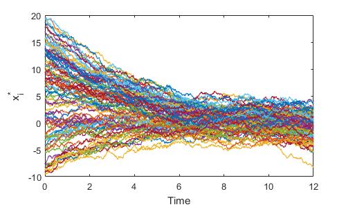
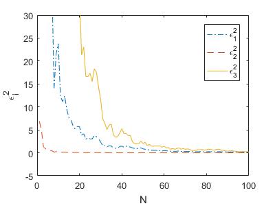
Figure 1. (a) is the trajectories of $x^{*}_{i}$, $i=1,\cdots,100$ and (b) is the curves of $\varepsilon_{i}^{2}$, $i=1,2,3$ when time interval is $[0,12]$.

7. Conclusion

This paper has analyzed the social optima in a class of LQ mean field control problem. We obtain the decentralized form of the optimal controls for the leader and $N$ followers. By Ricatti equation method, we discuss the solvability of the FBSDE. Finally, a Stackelberg equilibrium theorem is established. For future work, one can extend the results of this paper to the hierarchical control with many leaders case.

Appendix A Proof of Lemma 5

By (31) and (32), we have

$$\left\{\begin{aligned} &d(x^{*})^{(N)}=[A(x^{*})^{(N)}-BR^{-1}B^{T}p^{(N)}+C(x^{*})^{(N)}+Fx_{0}^{*}]dt+\frac{1}{N}\sum_{i=1}^{N}DdW_{i},\ (x^{*})^{(N)}(0)=\frac{1}{N}\sum_{i=1}^{N}\xi_{i},\\ &d\bar{x}^{(N)}=[A\bar{x}^{(N)}-BR^{-1}B^{T}p^{(N)}+C\hat{x}+F\bar{x}_{0}]dt+\frac{1}{N}\sum_{i=1}^{N}DdW_{i},\quad\bar{x}^{(N)}(0)=\frac{1}{N}\sum_{i=1}^{N}\xi_{i},\\ &dp^{(N)}=-[A^{T}p^{(N)}+\chi_{1}]dt+\zeta_{0}dW_{0}+\frac{1}{N}\sum_{i=1}^{N}\zeta_{i}dW_{i},\quad p^{(N)}(T)=Gx^{(N)}(T)+\chi_{2}.\\ \end{aligned}\right.$$ (42)

To prove Lemma 5, we need the following two lemmas. Assume that (A1)-(A4) hold. Let $\bar{x}^{(N)}=\frac{1}{N}\sum_{i=1}^{N}\bar{x}_{i}$ and $p^{(N)}=\frac{1}{N}\sum_{i=1}^{N}p_{i}$. Then

$$\sup_{0\leq t\leq T}\mathbb{E}\|\bar{x}^{(N)}-\hat{x}\|^{2}=O(\frac{1}{N}),\quad\sup_{0\leq t\leq T}\mathbb{E}\|p^{(N)}-\hat{p}\|^{2}=O(\frac{1}{N}).$$

Proof.

Combining (42) and (18), we can obtain

$$\left\{\begin{aligned} &d\mu_{1}=[A\mu_{1}-BR^{-1}B^{T}\mu_{2}]dt+\frac{1}{N}\sum_{i=1}^{N}DdW_{i},\quad\mu_{1}(0)=\frac{1}{N}\sum_{i=1}^{N}\xi_{i}-\hat{\xi},\\ &d\mu_{2}=-[A^{T}\mu_{2}+Q\mu_{1}+\frac{1}{N}\sum_{i=1}^{N}\zeta_{i}dW_{i},\quad\mu_{2}(T)=G\mu_{1},\\ \end{aligned}\right.$$

where $\mu_{1}=\bar{x}^{(N)}-\hat{x}$ and $\mu_{2}=p^{(N)}-\hat{p}$. Denote $\mu_{2}=P\mu_{1}+\varphi,\ t\in[0,T]$, where $P\in C^{1}([0,T];\mathbb{S}^{n})$ is the solution of the following Ricatti equation and $\varphi\in C^{1}([0,T];\mathbb{R}^{n})$ satisfies

$$\left\{\begin{aligned} &\dot{P}+PA-PBR^{-1}B^{T}P+A^{T}P+Q=0,\ t\in[0,T],\quad P(T)=G,\\ &d\varphi=-(A-BR^{-1}B^{T}P)^{T}\varphi dt+\frac{1}{N}\sum_{i=1}^{N}(PD-\zeta_{i})dW_{i},\ t\in[0,T],\quad\varphi(T)=0.\end{aligned}\right.$$

This is a standard Ricatti equation and the latter BSDE has a unique solution $\varphi=0,t\in[0,T]$. Thus $\mu_{2}=P\mu_{1}$ and

$$d\mu_{1}=[A-BR^{-1}B^{T}P]\mu_{1}dt+\frac{1}{N}\sum_{i=1}^{N}DdW_{i}.$$

By Cauchy-Schwarz inequality and Burkholder-Davis-Gundy’s inequality, we have

$$\sup_{0\leq t\leq T}\mathbb{E}\|\mu_{1}\|^{2}=\sup_{0\leq t\leq T}\mathbb{E}\bigg{\|}\int_{0}^{t}(A-BR^{-1}B^{T}P)\mu_{1}ds+\int_{0}^{t}\frac{1}{N}\sum_{i=1}^{N}DdW_{i}\bigg{\|}^{2}$$

$$\leq 2\sup_{0\leq t\leq T}\mathbb{E}\bigg{\|}\int_{0}^{t}(A-BR^{-1}B^{T}P)\mu_{1}ds\bigg{\|}^{2}+2\sup_{0\leq t\leq T}\mathbb{E}\bigg{\|}\int_{0}^{t}\frac{1}{N}\sum_{i=1}^{N}DdW_{i}\bigg{\|}^{2}$$

$$\leq 2K\bigg{\{}\sup_{0\leq t\leq T}\mathbb{E}\int_{0}^{t}\|\mu_{1}\|^{2}ds+\frac{1}{N^{2}}\sum_{i=1}^{N}\mathbb{E}\int_{0}^{T}\|D\|^{2}ds\bigg{\}}=2K\sup_{0\leq t\leq T}\mathbb{E}\int_{0}^{t}\|\mu_{1}\|^{2}ds+O(\frac{1}{N}),$$

where constant $K$ is independent of $N$. Then, by Gronwall’s inequality and $\mu_{2}=P\mu_{1}$, we obtain

$$\sup_{0\leq t\leq T}\mathbb{E}\|\mu_{1}\|^{2}=O(\frac{1}{N}),\quad\sup_{0\leq t\leq T}\mathbb{E}\|\mu_{2}\|^{2}=O(\frac{1}{N}).$$

The lemma follows. ∎

Assume that (A1)-(A4) hold. Let $(x^{*})^{(N)}=\frac{1}{N}\sum_{i=1}^{N}x^{*}_{i}$. Then

$$\sup_{0\leq t\leq T}\mathbb{E}\|x_{0}^{*}-\bar{x}_{0}\|^{2}=O(\frac{1}{N}),\quad\sup_{0\leq t\leq T}\mathbb{E}\|(x^{*})^{(N)}-\bar{x}^{(N)}\|^{2}=O(\frac{1}{N}).$$

Proof.

Denote $\mu_{3}=x_{0}^{*}-\bar{x}_{0}$ and $\mu_{4}=(x^{*})^{(N)}-\bar{x}^{(N)}$. By (42), we can obtain

$$d\left(\begin{array}[]{c}\mu_{3}\\ \mu_{4}\\ \end{array}\right)=\bigg{[}\left(\begin{array}[]{cc}A_{0}&C_{0}\\ F&A+C\\ \end{array}\right)\left(\begin{array}[]{c}\mu_{3}\\ \mu_{4}\\ \end{array}\right)+\left(\begin{array}[]{c}C_{0}\\ C\\ \end{array}\right)\mu_{1}\bigg{]}dt,\quad\left(\begin{array}[]{c}\mu_{3}\\ \mu_{4}\\ \end{array}\right)(0)=\left(\begin{array}[]{c}0\\ 0\\ \end{array}\right).$$

For some constant $K$ which is independent of $N$ such that

$$\sup_{0\leq t\leq T}\mathbb{E}\bigg{\|}\left(\begin{array}[]{c}\mu_{3}\\ \mu_{4}\\ \end{array}\right)\bigg{\|}^{2}=\sup_{0\leq t\leq T}\mathbb{E}\bigg{\|}\int_{0}^{t}\bigg{[}\left(\begin{array}[]{cc}A_{0}&C_{0}\\ F&A+C\\ \end{array}\right)\left(\begin{array}[]{c}\mu_{3}\\ \mu_{4}\\ \end{array}\right)+\left(\begin{array}[]{c}C_{0}\\ C\\ \end{array}\right)\mu_{1}\bigg{]}ds\bigg{\|}^{2}$$

$$\leq 2K\bigg{\{}\sup_{0\leq t\leq T}\mathbb{E}\int_{0}^{t}\bigg{\|}\left(\begin{array}[]{c}\mu_{3}\\ \mu_{4}\\ \end{array}\right)\bigg{\|}^{2}ds+\sup_{0\leq t\leq T}\mathbb{E}\int_{0}^{t}\|\mu_{1}\|^{2}ds\bigg{\}}=2K\sup_{0\leq t\leq T}\mathbb{E}\int_{0}^{t}\bigg{\|}\left(\begin{array}[]{c}\mu_{3}\\ \mu_{4}\\ \end{array}\right)\bigg{\|}^{2}ds+O(\frac{1}{N}).$$

By Gronwall’s inequality, one can obtain

$$\sup_{0\leq t\leq T}\mathbb{E}\bigg{\|}\left(\begin{array}[]{c}\mu_{3}\\ \mu_{4}\\ \end{array}\right)\bigg{\|}^{2}=O(\frac{1}{N}).$$

Thus, the lemma follows. ∎

Proof of Lemma 5.

Since

$$\|(x^{*})^{(N)}-\hat{x}\|^{2}=\|(x^{*})^{(N)}-\bar{x}^{(N)}+\bar{x}^{(N)}-\hat{x}\|^{2}\leq 2\|(x^{*})^{(N)}-\bar{x}^{(N)}\|^{2}+2\|\bar{x}^{(N)}-\hat{x}\|^{2}.$$

Combining Lemma A and Lemma A, it leads to

$$\mathbb{E}\int_{0}^{T}\|(x^{*})^{(N)}-\hat{x}\|^{2}dt+\mathbb{E}\int_{0}^{T}\|p^{(N)}-\hat{p}\|^{2}dt+\mathbb{E}\int_{0}^{T}\|x^{*}_{0}-\bar{x}_{0}\|^{2}dt\leq T\cdot O(\frac{1}{N})=O(\frac{1}{N}).$$

The lemma follows. ∎

Appendix B Proof of Lemma 5

Proof.

By (24), (42), (32) and using a similar argument in Lemma A, one obtain that for some constant $K$ which is not dependent on $N$ such that

$$\sup_{0\leq t\leq T}\mathbb{E}\|x_{0}^{*}\|^{2}\leq K,\quad\sup_{0\leq t\leq T}\mathbb{E}\|(x^{*})^{(N)}\|^{2}\leq K.$$

By Cauchy-Schwarz inequality and Burkholder-Davis-Gundy’s inequality, we obtain

$$\sup_{0\leq t\leq T}\mathbb{E}\|x^{*}_{i}\|^{2}=\sup_{0\leq t\leq T}\mathbb{E}\bigg{\|}\int_{0}^{t}(Ax^{*}_{i}-BR^{-1}B^{T}p_{i}+C(x^{*})^{(N)}+Fx^{*}_{0})ds+DdW_{i}\bigg{\|}^{2}$$

$$\leq \sup_{0\leq t\leq T}\mathbb{E}\int_{0}^{t}2\|Ax^{*}_{i}\|^{2}+2\|BR^{-1}B^{T}p_{i}\|^{2}+2\|C(x^{*})^{(N)}\|^{2}+2\|Fx^{*}_{0}\|^{2}ds+\sup_{0\leq t\leq T}\int_{0}^{t}2\|DdW_{i}\|^{2}$$

$$\leq 2\mathbb{E}\int_{0}^{T}\|Ax^{*}_{i}\|^{2}+\|BR^{-1}B^{T}p_{i}\|^{2}+\|C(x^{*})^{(N)}\|^{2}+\|Fx^{*}_{0}\|^{2}ds+\int_{0}^{T}\|D\|^{2}ds$$

$$\leq 2A^{2}\sup_{0\leq t\leq T}\mathbb{E}\int_{0}^{T}\|x^{*}_{i}\|^{2}ds+K,$$

where constants $K$ is independent of $N$. By Gronwall’s inequality, we have

$$\sup_{1\leq i\leq N}\big{[}\sup_{0\leq t\leq T}\mathbb{E}\|x^{*}_{i}\|^{2}\big{]}\leq K,$$

where $K$ is not dependent on $N$. Then, according to Cauchy-Schwarz inequality, Burkholder-Davis-Gundy’s inequality and the above discussion, we have

$$\mathcal{J}_{soc}^{(N)}(u_{0}^{*};u^{*})=\alpha N\mathcal{J}_{0}(u_{0}^{*};u^{*})+\sum_{i=1}^{N}\mathcal{J}_{i}(u_{0}^{*};u^{*})$$

$$= \alpha N\mathbb{E}\bigg{\{}\int_{0}^{T}\big{[}\|x_{0}^{*}-\Theta_{0}(x^{*})^{(N)}-\eta_{0}\|_{Q_{0}}^{2}+\|-(\alpha R_{0})^{-1}B_{0}^{T}y_{0}^{*}\|_{R_{0}}^{2}\big{]}dt+\|x_{0}^{*}(T)$$

$$-\hat{\Theta}_{0}(x^{*})^{(N)}(T)-\hat{\eta}_{0}\|_{G_{0}}^{2}\bigg{\}}+\sum_{i=1}^{N}\mathbb{E}\bigg{\{}\int_{0}^{T}\big{[}\|x_{i}^{*}-\Theta(x^{*})^{(N)}(t)-\Theta_{1}x_{0}^{*}-\eta\|_{Q}^{2}$$

$$+\|-R^{-1}B^{T}p_{i}\|_{R}^{2}\big{]}dt+\|x_{i}^{*}(T)-\hat{\Theta}(x^{*})^{(N)}(T)-\hat{\Theta}_{1}x_{0}^{*}(T)-\hat{\eta}\|_{G}^{2}\bigg{\}}\leq NK,$$

where $K$ is independent of $N$. The lemma follows. ∎

Appendix C Proof of Proposition 5 and 5

Proof of Proposition 5.

Since

$$\left\{\begin{aligned} &d\delta x_{0}=(A_{0}\delta x_{0}+C_{0}\delta x^{(N)})dt,\quad\delta x_{0}(0)=0,\\ &d\delta x^{(N)}=[(A+C)\delta x^{(N)}+\frac{B}{N}\delta u_{i}]dt,\quad\delta x^{(N)}(0)=0,\end{aligned}\right.$$

and by Proposition 5, we have $\|\delta u_{i}\|_{L^{2}}^{2}\leq K$, $K$ is independent of $N$. Using Cauchy-Schwarz inequality, it follows that

$$\mathbb{E}\sup_{0\leq s\leq t}\|\delta x^{(N)}\|^{2}= \mathbb{E}\sup_{0\leq s\leq t}\Big{\|}\int_{0}^{s}[(A+C)\delta x^{(N)}+\frac{B}{N}\delta u_{i}]dr\Big{\|}^{2}$$

$$\leq K\mathbb{E}\int_{0}^{t}\|\delta x^{(N)}\|^{2}dr+\frac{1}{N^{2}}\|K\|^{2}dr\leq K\mathbb{E}\int_{0}^{t}\|\delta x^{(N)}\|^{2}dr+O\Big{(}\frac{1}{N^{2}}\Big{)},$$

where $K$ is independent of $N$. By Gronwall’s inequality

$$\mathbb{E}\sup_{0\leq t\leq T}\|\delta x^{(N)}\|^{2}=O\Big{(}\frac{1}{N^{2}}\Big{)}.$$

For $\delta x_{0}$, we have

$$\mathbb{E}\sup_{0\leq s\leq t}\|\delta x_{0}\|^{2}= \mathbb{E}\sup_{0\leq s\leq t}\Big{\|}\int_{0}^{s}[A_{0}\delta x_{0}+C_{0}\delta x^{(N)}]dr\Big{\|}^{2}\leq K\mathbb{E}\int_{0}^{t}\|\delta x_{0}\|^{2}dr+O\Big{(}\frac{1}{N^{2}}\Big{)},$$

where $K$ is independent of $N$. By Gronwall’s inequality

$$\mathbb{E}\sup_{0\leq t\leq T}\|\delta x_{0}\|^{2}=O\Big{(}\frac{1}{N^{2}}\Big{)}.$$

Moreover,

$$\Theta^{T}Q(\bar{x}_{i}-\Theta\bar{x}^{(N)}-\Theta_{1}\bar{x}_{0}-\eta)\leq\frac{1}{N}\inf_{(u_{0};u)}J_{soc}^{(N)}(u_{0};u)\leq K.$$

Similarly, $\Theta_{1}^{T}Q(\bar{x}_{i}-\Theta\bar{x}^{(N)}-\Theta_{1}\bar{x}_{0}-\eta)$, $\hat{\Theta}^{T}G(\bar{x}_{i}(T)-\hat{\Theta}\bar{x}^{(N)}(T)-\hat{\Theta}_{1}\bar{x}_{0}(T)-\hat{\eta})$, $\hat{\Theta}_{1}^{T}G(\bar{x}_{i}(T)-\hat{\Theta}\bar{x}^{(N)}(T)-\hat{\Theta}_{1}\bar{x}_{0}(T)-\hat{\eta})$ are bounded. Thus,

$$\langle\Theta^{T}Q(\bar{x}_{i}-\Theta\bar{x}^{(N)}-\Theta_{1}\bar{x}_{0}-\eta),\delta x^{(N)}\rangle+\langle\Theta_{1}^{T}Q(\bar{x}_{i}-\Theta\bar{x}^{(N)}-\Theta_{1}\bar{x}_{0}-\eta),\delta x_{0}\rangle+\langle\hat{\Theta}^{T}G(\bar{x}_{i}(T)-\hat{\Theta}\bar{x}^{(N)}(T)$$

$$-\hat{\Theta}_{1}\bar{x}_{0}(T)-\hat{\eta}),\delta x^{(N)}(T)\rangle+\langle\hat{\Theta}_{1}^{T}G(\bar{x}_{i}(T)-\hat{\Theta}\bar{x}^{(N)}(T)-\hat{\Theta}_{1}\bar{x}_{0}(T)-\hat{\eta}),\delta x_{0}(T)\rangle=o(1).$$

The proposition follows. ∎

Proof of Proposition 5.

Since

$$\left\{\begin{aligned} &d(\sum_{j\neq i}\delta x_{j})=[A(\sum_{j\neq i}\delta x_{j})+C\frac{N-1}{N}\delta x^{(N)}+F(N-1)\delta x_{0}]dt,\quad(\sum_{j\neq i}\delta x_{j})(0)=0,\\ &d(N\delta x_{0})=[A_{0}(N\delta x_{0})+C_{0}(N\delta x^{(N)})]dt,\quad(N\delta x_{0})(0)=0,\\ &d(N\delta x_{j})=[A(N\delta x_{j})+C(N\delta x^{(N)})+F(N\delta x_{0})]dt,\quad(N\delta x_{j})(0)=0.\\ \end{aligned}\right.$$

According to equations in (6), one can obtain

$$\left\{\begin{aligned} &d(N\delta x_{j}-\sum_{j\neq i}\delta x_{j})=[A(N\delta x_{j}-\sum_{j\neq i}\delta x_{j})+\frac{C}{N}\delta x^{(N)}+F\delta x_{0}]dt,\ (N\delta x_{j}-\sum_{j\neq i}\delta x_{j})(0)=0,\\ &d(N\delta x_{0}-\delta x_{0}^{\dagger})=[A_{0}(N\delta x_{0}-\delta x_{0}^{\dagger})+C_{0}(N\delta x_{j}-\sum_{j\neq i}\delta x_{j})+C_{0}(N\delta x_{j}-d\delta x^{\dagger})]dt,\ (N\delta x_{0}-\delta x_{0}^{\dagger})(0)=0,\\ &d(N\delta x_{j}-\delta x^{\dagger})=[(A+C)(N\delta x_{j}-\delta x^{\dagger})+C(N\delta x_{j}-\sum_{j\neq i}\delta x_{j})+F(N\delta x_{0}-\delta x_{0}^{\dagger})]dt,\ (N\delta x_{j}-\delta x^{\dagger})(0)=0.\\ \end{aligned}\right.$$

Combing with the results in Proposition 5, we have

$$\mathbb{E}\sup_{0\leq s\leq t}\|N\delta x_{j}-\sum_{j\neq i}\delta x_{j}\|^{2}= \mathbb{E}\sup_{0\leq s\leq t}\Big{\|}\int_{0}^{s}[A(N\delta x_{j}-\sum_{j\neq i}\delta x_{j})+\frac{C}{N}\delta x^{(N)}+F\delta x_{0}]dr\Big{\|}^{2}$$

$$\leq K\mathbb{E}\int_{0}^{t}\|N\delta x_{j}-\sum_{j\neq i}\delta x_{j}\|^{2}dr+O\Big{(}\frac{1}{N^{2}}\Big{)},$$

where constant $K$ is independent of $N$. By Gronwall’s inequality

$$\mathbb{E}\sup_{0\leq t\leq T}\|N\delta x_{j}-\sum_{j\neq i}\delta x_{j}\|^{2}=O(\frac{1}{N^{2}}).$$

Since $N\delta x_{0}-\delta x_{0}^{\dagger}$ and $N\delta x_{j}-\delta x^{\dagger}$ are coupled, we have

$$\mathbb{E}\sup_{0\leq s\leq t}\Bigg{\|}\left(\begin{array}[]{c}N\delta x_{0}-\delta x_{0}^{\dagger}\\ N\delta x_{j}-d\delta x^{\dagger}\\ \end{array}\right)\Bigg{\|}^{2}$$

$$= \mathbb{E}\sup_{0\leq s\leq t}\Bigg{\|}\int_{0}^{s}\Bigg{[}\left(\begin{array}[]{cc}A_{0}&C_{0}\\ F&A+C\\ \end{array}\right)\left(\begin{array}[]{c}N\delta x_{0}-\delta x_{0}^{\dagger}\\ N\delta x_{j}-d\delta x^{\dagger}\\ \end{array}\right)+\left(\begin{array}[]{c}C_{0}\\ C\\ \end{array}\right)(N\delta x_{j}-\sum_{j\neq i}\delta x_{j})\Bigg{]}dr\Bigg{\|}^{2}$$

$$\leq K\mathbb{E}\int_{0}^{t}\Bigg{\|}\left(\begin{array}[]{c}N\delta x_{0}-\delta x_{0}^{\dagger}\\ N\delta x_{j}-d\delta x^{\dagger}\\ \end{array}\right)\Bigg{\|}^{2}dr+O\Big{(}\frac{1}{N^{2}}\Big{)},$$

where real-valued matrix $K$ is independent of $N$. By Gronwall’s inequality

$$\mathbb{E}\sup_{0\leq t\leq T}\Bigg{\|}\left(\begin{array}[]{c}N\delta x_{0}-\delta x_{0}^{\dagger}\\ N\delta x_{j}-d\delta x^{\dagger}\\ \end{array}\right)\Bigg{\|}^{2}=O\Big{(}\frac{1}{N^{2}}\Big{)}.$$

The proposition follows. ∎

References

- [1] T. Başar, A. Bensoussan and S. P. Sethi, Differential games with mixed leadership: the open-loop solution. Appl. Math. Comput. 217 (2010) 972-979.
- [2] T. Başar and G. J. Olsder, Dynamic Noncooperative Game Theory. SIAM, Philadelphia (1999).
- [3] M. Bardi and F. S. Priuli, Linear-quadratic -person and mean-field games with ergodic cost. SIAM J. Control Optim. 52 (2014) 3022-3052.
- [4] C. T. Bauch and D. J. D. Earn, Vaccination and the theory of games. P. Natl. Acad. Sci. USA. 101 (2004) 13391-13394.
- [5] D. Bauso and R. Pesenti, Team theory and person-by-person optimization with binary decisions. SIAM J. Control Optim. 50 (2012) 3011-3028.
- [6] A. Bensoussan, M. H. M. Chau and S. C. P. Yam, Mean field games with a dominating player. Appl. Math. Optim. 74 (2016) 91-128.
- [7] A. Bensoussan, J. Frehse and P. Yam, Mean Field Games and Mean Field Type Control Theory. Springer, New York (2013).
- [8] P. E. Caines, Mean field games, in Encyclopedia of Systems and Control, Ed. T. Samad and J. Baillieul, Springer-Verlag, Berlin (2014).
- [9] R. Carmona and F. Delarue, Probabilistic analysis of mean-field games. SIAM J. Control Optim. 51 (2013) 2705-2734.
- [10] R. Carmona, F. Delarue and D. Lacker, Mean field games with common noise. Ann. Probab. 44 (2016) 3740-3803.
- [11] R. Carmona and P. Wang, Finite state mean field games with major and minor players. arXiv: 1610.05408.
- [12] R. Carmona and X. Zhu, A probabilistic approach to mean field games with major and minor players. Ann. Appl. Probab. 26 (2016) 1535-1580
- [13] R. Couillet, S. M. Perlaza, H. Tembine and M. Debbah, Electrical vehicles in the smart grid: a mean field game analysis. IEEE. J. Sel. Area. Comm. 30 (2012) 1086-1096.
- [14] D. Firoozi and P. E. Caines, Mean field game -Nash equilibria for partially observed optimal execution problems in finance. Proc. the IEEE 55th Conference on Decision and Control. Las Vegas (2016) 268-275.
- [15] G. Gnecco, M. Sanguineti and M. Gaggero, Suboptimal solutions to team optimization problems with stochastic information structure. SIAM J. Optimiz. 22 (2012) 212-243.
- [16] T. Groves, Incentives in teams. Econometrica, 41 (1973) 617-631.
- [17] Y. C. Ho and K. C. Chu, Team decision theory and information structures in optimal control Part I. IEEE Trans. Automat. Contr. 17 (1972) 15-22.
- [18] J. Huang and M. Huang, Robust mean field linear-quadratic-Gaussian games with unknown -disturbance. SIAM J. Control Optim. 55 (2017) 2811-2840.
- [19] J. Huang and N. Li, Linear quadratic mean-field game for stochastic delayed systems. IEEE Trans. Automat. Contr. 63 (2018) 2722-2729.
- [20] J. Huang, S. Wang and Z. Wu, Backward-forward linear-quadratic mean-field games with major and minor agents. Probability, Uncertainty and Quantitative Risk 1 (2016) 1-27.
- [21] M. Huang, P. E. Caines and R. P. Malhamé, Individual and mass behaviour in large population stochastic wireless power control problems: centralized and Nash equilibrium solutions. Proc. 42nd IEEE International Conference on Decision and Control. Maui (2003) 98-103.
- [22] M. Huang, P. E. Caines and R. P. Malhamé, Social optima in mean-field LQG control: centralized and decentralized strategies. IEEE Trans. Automat. Contr. 57 (2012) 1736-1751.
- [23] M. Huang and S. L. Nguyen, Linear-quadratic mean field teams with a major agent. Proc. IEEE 55th Conference on Decision and Control. Las Vegas (2016) 6958-6963.
- [24] A. C. Kizilkale and R. P. Malhame, Collective target tracking mean field control for Markovian jump-driven models of electric water heating loads. Proc. the 19th IFAC World Congress. Cape Town, South Africa (2014) 1867-1972.
- [25] J. Lasry and P. Lions, Mean field games. Jpn. J. Math. 2 (2007) 229-260.
- [26] T. Li and J. Zhang, Asymptotically optimal decentralized control for large population stochastic multiagent systems. IEEE Trans. Automat. Contr. 53 (2008) 1643-1660.
- [27] Y. N. Lin, X. S. Jiang, and W. H. Zhang, An open-loop Stackelberg strategy for the linear quadratic mean-field stochastic differential game. IEEE Trans. Automat. Contr. 64 (2019) 97-110.
- [28] J. Ma and J. Yong, Forward-Backward Stochastic Differential Equations and their Applications. Springer-Verlag, Berlin (1999).
- [29] S. Maharjan, Q. Zhu, Y. Zhang, S. Gjessing and T. Basar, Dependable demand response management in the smart grid: a Stackelberg game approach. IEEE Trans. Smart Grid. 4 (2013) 120-132.
- [30] J. Marschak, Elements for a theory of teams. Manage Sci. 1 (1955) 127-137.
- [31] J. Moon and T. Başar, Linear quadratic mean field Stackelberg differential games. Automatica 97 (2018) 200-213.
- [32] S. L. Nguyen and M. Huang, Linear-quadratic-Gaussian mixed games with continuum-parametrized minor players. SIAM J. Control Optim. 50 (2012) 2907-2937.
- [33] M. Nourian and P. E. Caines, -Nash mean field game theory for nonlinear stochastic dynamical systems with major and minor agents. SIAM J. Control Optim. 51 (2013) 3302-3331.
- [34] J. Shi, G. Wang and J. Xiong, Leader-follower stochastic differential game with asymmetric information and applications. Automatica 63 (2016) 60-73.
- [35] M. Simaan and J. Cruz, A Stackelberg solution for games with many players. IEEE Trans. Automat. Contr. 18 (1973) 322-324.
- [36] H. Tembine, Q. Zhu and T. Başar, Risk-sensitive mean-field games. IEEE Trans. Automat. Contr. 59 (2014) 835-850.
- [37] B. Wang and J. Zhang, Mean field games for large population multiagent systems with Markov jump parameters. SIAM J. Control Optim. 50 (2012) 2308-2334.
- [38] B. Wang and J. Zhang, Hierarchical mean field games for multiagent systems with tracking-type costs: distributed -Stackelberg equilibria. IEEE Trans. Automat. Contr. 59 (2014) 2241-2247.
- [39] B. Wang and J. Zhang, Social optima in mean field linear-quadratic-Gaussian models with Markov jump parameters. SIAM J. Control Optim. 55 (2017) 429-456.
- [40] B. Wang and J. Huang, Social optima in robust mean field LQG control. Proc. the 11th Asian Control Conference. Gold Coast, QLD (2017) 2089-2094.
- [41] G. Y. Weintraub, C. L. Benkard and B. V. Roy, Markov perfect industry dynamics with many firms. Econometrica 76 (2008) 1375-1411.
- [42] J. Yong, Linear forward-backward stochastic differential equations. Appl. Math. Optim. 39 (1999) 93-119.
- [43] J. Yong, A leader-follower stochastic linear quadratic differential game. SIAM J. Control Optim. 41 (2002) 1015-1041.
- [44] J. Yong and X. Y. Zhou, Stochastic Controls: Hamiltonian Systems and HJB Equations. Springer-Verlag. New York (1999).