Cross-study Learning
for Generalist and Specialist Predictions

Abstract

The integration and use of data from multiple studies, for the development of prediction models is an important task in several scientific fields. We propose a framework for generalist and specialist predictions that leverages multiple datasets, with potential differences in the relationships between predictors and outcomes. Our framework uses stacking, and it includes three major components: 1) an ensemble of prediction models trained on one or more datasets, 2) task-specific utility functions and 3) a no-data-reuse technique for estimating stacking weights. We illustrate that under mild regularity conditions the framework produces stacked PFs with oracle properties. In particular we show that the the stacking weights are nearly optimal. We also characterize the scenario where the proposed no-data-reuse technique increases prediction accuracy compared to stacking with data reuse in a special case. We perform a simulation study to illustrate these results. We apply our framework to predict mortality using a collection of datasets on long-term exposure to air pollutants.

1 Introduction

It is increasingly common for researchers to have access to multiple ($K>1$) studies and datasets to answer the same or strictly related scientific questions (Klein et al., 2014; Kannan et al., 2016; Manzoni et al., 2018). Although datasets from multiple studies may contain the same outcome variable $Y$ and covariates $X$ (for example, patient survival and pre-treatment prognostic profiles in clinical studies), the $(X,Y)$ joint distributions $P_{1},\ldots,P_{K}$ are typically different, due to distinct study populations, study designs and technological artifacts (Simon et al., 2003; Rhodes et al., 2004; Patil et al., 2015; Sinha et al., 2017). In this article, we discuss the task of developing prediction models using multiple datasets, accounting for potential differences between the $(P_{k},k=1,\ldots,K)$ study-specific distributions. In this multi-study setting we focus on two classes of prediction functions (PFs) which have distinct goals: generalist and specialist PFs.

Generalist predictions are directed toward studies $(K+1,K+2,\ldots)$ that are not included in the available data collection. The strategy to develop a generalist PF depends on relations and similarities between studies. For example, the study-specific geographic areas or assays can be relevant in the development of prediction models. If studies are considered exchangeable, i.e. joint analyses are invariant to permutations of the study indices $k$, then a model which consistently predicts accurately across all $K$ available studies is a good candidate for generalist use to predict $Y$ in other studies $k>K$. Generalist PFs have been studied in the literature (Sutton and Higgins, 2008; Tseng et al., 2012; Pasolli et al., 2016) and several contributions are based on hierarchical models (Warn et al., 2002; Babapulle et al., 2004; Higgins et al., 2009). If the exchangeability assumption is inadequate, then joint models for multiple studies can incorporate information on relevant relations between studies (Moreno-Torres et al., 2012). For example, when $K$ datasets are representative of different time points $t_{1}<t_{2}<...<t_{K}$, one can incorporate potential cycles or long-term trends.

Specialist predictions are directed to predict future outcomes $Y$ based on predictors $X$ in the context of a specific study $k\in\{1,\ldots K\}$—for example a geographic area—represented by one of the $K$ datasets. Bayesian models can be used to borrow information and leverage the other $(K-1)$ datasets in addition to the $k$-th dataset. Typically the degree of homogeneity of the distributions $(P_{1},\ldots,P_{K})$ correlates with the accuracy improvements that one achieves with multi-study models compared to models developed using only data from a single study $k$.

Recently, the use of ensemble methods has been proposed to develop generalist PFs based on multi-study data collections (Patil and Parmigiani, 2018; Zhang et al., 2019; Loewinger et al., 2019). In particular stacking (Wolpert, 1992; Breiman, 1996) has been used to combine PFs $\{\hat{Y}_{k}(\cdot),\;k=1,\ldots,K\}$, each trained on a single study $k$, into a single generalist PF, $\hat{Y}(\cdot)=\sum_{k=1}^{K}w_{k}\times\hat{Y}_{k}(\cdot)$. The weights $w$ assigned to each model $\hat{Y}_{k}$ in stacking are often selected by maximizing a utility function representative of the accuracy of the resulting PF. In this manuscript our focus will be on collections of exchangeable studies. Nonetheless, the application of stacking does not require exchangeability, and the optimization of the ensemble weights can be tailored to settings where exchangeabilty is implausible.

Stacking allows investigators to capitalize on multiple machine learning algorithms, such as random forest or neural networks, to train the study-specific functions $\hat{Y}_{k}$. We investigate the optimization of the ensemble weights assigned to a collection of single-set prediction functions (SPFs) generated with arbitrary machine learning methods. Each SPF is trained by a single study $k$ or combining a subset of studies into a single data matrix. These SPFs can be trained using different algorithms and models. The ensemble weights approximately maximize a utility function $U$, which we estimate using the entire collection of $K$ studies.

Stacking in multi-study settings can potentially suffer from over-fitting due to data reuse (DR): the same datasets generate SPFs and contribute to the optimization of the stacking weights $w$. With the aim of mitigating overfitting we introduce no data reuse (NDR) procedures that include three key components: the development of SPFs, the estimation of the utility function $U$, and selection of the ensemble weights $w$. We compare DR and NDR procedures to weight SPFs. In this comparison we will use mean squared error (MSE) as primary metric to evaluate accuracy. Our results show that, when the number of studies $K$ and the sample sizes $n_{k}$ become large, both DR and NDR stacking achieve a performance similar to an asymptotic oracle benchmark. The asymptotic oracle is defined as the linear combination of the SPFs’ limits {$\lim\limits_{n_{k}\to\infty}\hat{Y}_{k};k=1,\ldots,K\}$ that minimizes the MSE in future studies $k>K$. Our results bound the MSE difference between the oracle ensemble and the two stacking procedures, with and without DR. Related bounds have been studied in the single-study setting (van der Laan et al., 2006) and in the functional aggregation literature (Juditsky and Nemirovski, 2000; Juditsky et al., 2008). We also characterize in a special case under which circumstance NDR stacking has better performance than DR stacking.

We apply our NDR and DR stacking procedures to predict mortality in Medicare beneficiaries enrolled before 2002. The datasets contain health-related information of the beneficiaries at the zipcode-level and measurements of air pollutants. We are interested in predicting the number of deaths per 10,000 person-years. In distinct analyses, we partitioned the database into state-specific datasets ($K=49$) and the data from California into county-specific datasets ($K=57$). We compare the relative performance of NDR and DR stacking.

2 Generalist and Specialist Predictions

2.1 Notation

We use data from $K$ studies $k=1,\ldots,K$, with sample sizes $n_{k}$. For individual $i$ in study $k$ we have a vector of $p$-dimensional characteristics $x_{i,k}\in\mathcal{X}\subset\mathbb{R}^{p}$ and the individual outcome $y_{i,k}\in\mathbb{R}$. Let $\mathcal{S}_{k}=\{(x_{i,k},y_{i,k}),i=1,\ldots,n_{k}\}$ denote all data from study $k$ and $\mathcal{S}=\{\mathcal{S}_{k},k=1,\ldots,K\}$ the collection of all $K$ datasets. We define a list of training sets (LTS), denoted as $\mathcal{D}$, which includes $T$ members $D_{1},\ldots,D_{T}$. Each $D_{t}$ is a set of $(i,k)$ indices, where $i\in\{1,2,\ldots,n_{k}\}$ is the sample index within a study $k$. The set $D_{t}$ can include indices with different $k$ values (see for example $D_{3}$ in Figure 1). We use $D^{(s)}_{k}=\{(1,k),\ldots,(n_{k},k)\}$ to denote the set of all indices in study $k$. We call a collection $\mathcal{D}$ study-specific if $T=K$ and $D_{t}=D^{(s)}_{t},t=1,\ldots,K$.

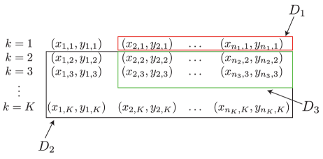
Figure 1: A representation of studies and training sets in the LTS $\mathcal{D}=\{D_{1},D_{2},D_{3}\}.$

We consider $L$ different learners/algorithms—a learner is a method for generating a PF—such as linear regression, random forests or neural networks. Training the learner $\ell$ on $D_{t}\in\mathcal{D}$ generates an SPF denoted as $\hat{Y}_{t}^{\ell}:\mathcal{X}\to\mathbb{R}$. The set of SPFs is $\hat{\mathcal{Y}}=\{\hat{Y}_{t}^{\ell}(\cdot);\ell=1,\ldots,L,\;t=1,\ldots,T\}$. Let $W$ be a subset of $\mathbb{R}^{TL}$. With stacking (Wolpert, 1992) we combine the components of $\hat{\mathcal{Y}}$ into $\hat{Y}_{w}:\mathcal{X}\to\mathbb{R}$,

$$\hat{Y}_{w}(\cdot)=\sum_{\ell=1}^{L}\sum_{t=1}^{T}w_{\ell,t}\hat{Y}_{t}^{\ell}(\cdot),$$ (1)

where $w=(w_{\ell,t};\ell\leq L,t\leq T)$ is a vector of weights in $W$.

We want to use $\hat{Y}_{w}$ for prediction in a target population with unknown joint $(X,Y)$ distribution $\pi$. The accuracy of $\hat{Y}_{w}$ is quantified by its expected utility $U$, a summary of accuracy in the target population:

$$U(w;\pi)=\int_{(x,y)}u(\hat{Y}_{w}(x),y)\;d\pi(x,y),$$

where $u(y,y^{\prime})$ is a utility function, e.g. the negative squared difference $u(y,y^{\prime})=-(y-y^{\prime})^{2}$. Here $\pi$ is unknown and one can estimate $U(w;\pi)$ with

$$\hat{U}^{\text{DR}}(w;\nu)=\sum_{k=1}^{K}\frac{\nu_{k}}{n_{k}}\sum_{i=1}^{n_{k}}u(\hat{Y}_{w}(x_{i,k}),y_{i,k}),$$ (2)

where DR indicates that the estimate of $U$ involves DR. See Section 3 for a discussion of DR.

The weights $\nu_{k}\geq 0$, $\sum_{k}\nu_{k}=1$, are user-specified and represent the relation between the target $\pi$ and the set of populations $P_{1},\ldots,P_{K}$. In this paper, we are interested in generalist prediction which, under the assumption of exchangeable studies, is compatible with $\nu_{k}=\frac{1}{K}$, for $k=1,\ldots,K$, and specialist prediction, which corresponds to $\nu_{k}=1$ for study $k\in\{1,\ldots,K\}$ and 0 for the remaining $K-1$ studies.

2.2 Generalist prediction

Generalist prediction are applicable to future studies $K+1,K+2,\ldots$. Therefore the expected utility of a generalist PF $\hat{Y}_{w}$ can be represented as

$$U_{g}(w)=\lim_{I\to\infty}I^{-1}\sum_{i=1}^{I}U(w;P_{K+i}).$$

We will consider scenarios where the above limit is well defined. If $P_{1},P_{2},\ldots$, are exchangeable, i.e. there exists $Q$ such that $P_{k}|Q\overset{iid}{\sim}Q$ for $k=1,2,\ldots,$ then $U_{g}(w)$ can be rewritten as

$$U_{g}(w)=\int\left[\int_{(x,y)}u(\hat{Y}_{w}(x),y)\mathop{}\!\mathrm{d}P(x,y)\right]\mathop{}\!\mathrm{d}Q.$$

Changing the order of integration,

$$U_{g}(w)=\int_{(x,y)}u(\hat{Y}_{w}(x),y)\mathop{}\!\mathrm{d}P_{0}(x,y),$$

where $P_{0}$ is the mean of $Q$, i.e. $P_{0}(\cdot)=\int P(\cdot)dQ$.

The target population is $P_{0}$. We can use $\nu_{k}=1/K$ for $k=1,\ldots,K$ in expression (2) to approximate $U_{g}(w)$. Note that in several applications the sequence $P_{1},P_{2}\ldots$ is not exchangeable. For example, in some data collections Markov relations $[P_{k}|P_{1},\ldots,P_{k-1}]\buildrel d\over{=}[P_{k}|P_{k-1}]$ constitute a suitable assumption(Shumway and Stoffer, 2017). Throughout this manuscript we will not specify $Q$, but we will assume the exchangeability of $P_{1},P_{2},\ldots$.

2.3 Specialist prediction

The target distribution $\pi$ coincides with $P_{k}$, for a single $k\in\{1,2,\ldots,K\}$. The expected utility of a specialist PF is

$$U_{s}(w;k)=U(w;P_{k})=\int_{(x,y)}u(\hat{Y}_{w}(x),y)\mathop{}\!\mathrm{d}P_{k}(x,y).$$

One can use the empirical distribution of study $k$ to estimate $P_{k}$. This is equivalent to set $\nu_{i}=1$ for $i=k$, and 0 otherwise in (2).

3 Generalist and specialist stacking

We use stacking for generalist and specialist predictions in the multi-study setting. We indicate as oracle weights

$$w_{g}=\operatorname*{arg\,max}_{w\in W}U_{g}(w),$$

$$w_{s}^{(k)}=\operatorname*{arg\,max}_{w\in W}U_{s}(w;k).$$

Let $w_{g;t,\ell}$ and $w_{s;t,\ell}^{(k)}$ denote the oracle weights for $\hat{Y}_{t}^{\ell}$ in generalist and specialist predictions. In this manuscript, if not otherwise specified, $u(y,y^{\prime})=-(y-y^{\prime})^{2}$.

Note that constraints (i.e., $w\in W\subset\mathbb{R}^{TL}$) on or penalties applied to select $w$ can lead to identical results. Indeed, in several optimization problems constraining a $K\times L-$dimensional parameter, e.g., $w\in W=\{w:\|w\|_{2}\leq c\}$, where $\|\cdot\|_{2}$ is the $L_{2}$ norm in the Euclidean space, is equivalent to the unconstrained optimization with an $L_{2}$ penalty on $w$. The use of penalties in the estimation of stacking weights has been discussed in Breiman (1996) and LeBlanc and Tibshirani (1996).

We introduce three different stacking approaches: DR stacking, within-study cross-validated stacking ($\text{CV}_{\text{ws}}$) and cross-set cross-validated stacking ($\text{CV}_{\text{cs}}$). The latter two are NDR stacking approaches. These three approaches select $w$ by maximizing distinct estimates of the utility functions $U_{g}(w)$ or $U_{s}(w;k)$. We discuss the estimators of $U_{g}(w)$ and $U_{s}(w;k)$ obtained with DR, $\text{CV}_{\text{ws}}$ and $\text{CV}_{\text{cs}}$. In two examples we derive the means and variances of the deviations of these estimates to the oracle. We illustrate that DR stacking and $\text{CV}_{\text{ws}}$ typically over-estimate the utility function $U$ with smaller variance compared to $\text{CV}_{\text{cs}}$, which tends to under-estimate $U$.

3.1 DR stacking

A direct approach to select $w$ for generalist and specialist predictions consists in optimizing the $\hat{U}^{\text{DR}}(w;\nu)$ estimates of $U_{g}(w)$ and $U_{s}(w;k)$. When the studies are exchangeable, $\operatorname*{arg\,max}_{w}\hat{U}^{\text{DR}}(w;\mathbf{1}_{K}/K)$ can be used for generalist predictions. Similarly, if we develop a specialist PF for study $k$, we can optimize $\hat{U}^{\text{DR}}(w;e_{k})$, where $e_{k}$ is a $K-$dimensional vector with the $k$-th component equal to one and all others zero. Let $\hat{w}^{\text{DR}}_{\nu}=\operatorname*{arg\,max}_{w\in W}\hat{U}^{\text{DR}}(w;\nu)$ and $\hat{Y}^{\text{DR}}_{\nu}=\sum_{\ell,t}\hat{w}^{\text{DR}}_{\nu;\ell,t}\hat{Y}_{t}^{\ell}$.

Training the SPF $\hat{Y}^{\ell}_{t}$ uses part of the data, i.e., $D_{t}$, that is later re-used to compute $\hat{U}^{\text{DR}}(w;\nu)$. To illustrate the effect of DR, we investigate the difference between $U_{g}(w)$ and $\hat{U}^{\text{DR}}(w;\nu)$:

$$\hat{U}^{\text{DR}}(w;\nu)-U_{g}(w)=-w^{\intercal}(\hat{\Sigma}^{\text{DR}}_{\nu}-\Sigma_{g})w+2w^{\intercal}(\hat{b}^{\text{DR}}_{\nu}-b_{g})+C$$ (3)

where $C$ is a constant. $\hat{\Sigma}^{\text{DR}}_{\nu}$ and $\Sigma_{g}$ are $TL\times TL$ matrices and their components corresponding to $w_{t,\ell}\times w_{t^{\prime},\ell^{\prime}}$ are

$$\hat{\Sigma}^{\text{DR}}_{\nu;t,t^{\prime},\ell,\ell^{\prime}}=\sum_{k}\frac{\nu_{k}}{n_{k}}\sum_{i}\hat{Y}_{t}^{\ell}(x_{i,k})\hat{Y}_{t^{\prime}}^{\ell^{\prime}}(x_{i,k}),\text{ and }\Sigma_{g;t,t^{\prime},\ell,\ell^{\prime}}=\langle\hat{Y}_{t}^{\ell},\hat{Y}_{t^{\prime}}^{\ell^{\prime}}\rangle,$$

where $\langle\hat{Y},\hat{Y}^{\prime}\rangle=\int_{x}\hat{Y}(x)\hat{Y}^{\prime}(x)\mathop{}\!\mathrm{d}P_{0}(x)$. Both $\hat{b}^{\text{DR}}_{\nu}$ and $b_{g}$ are $TL$-dimensional vectors, and the components correspond to $w_{t,\ell}$ are

$$\hat{b}^{\text{DR}}_{\nu;t,\ell}=\sum_{i,k}\frac{\nu_{k}}{n_{k}}\hat{Y}^{\ell}_{t}(x_{i,k})y_{i,k},\text{ and }b_{g;t,\ell}=\langle\hat{Y}_{t}^{\ell},y\rangle.$$

Here $\langle\hat{Y},y\rangle=\int_{x,y}y\hat{Y}(x)\mathop{}\!\mathrm{d}P_{0}(x,y)$. When $K\geq 3$, one can construct unbiased estimators of $\Sigma_{g;t,t^{\prime},\ell,\ell^{\prime}}$ and $b_{g;t,\ell}$. For example, $(K-2)^{-1}\sum\limits_{k\notin\{t,t^{\prime}\}}n_{k}^{-1}\sum_{i}\hat{Y}_{t}^{\ell}(x_{i,k})\hat{Y}_{t^{\prime}}^{\ell^{\prime}}(x_{i,k})$ is an unbiased estimator of $\Sigma_{g;t,t^{\prime},\ell,\ell^{\prime}}$.

We call $-w^{\intercal}(\hat{\Sigma}^{\text{DR}}_{\nu}-\Sigma_{g})w+2w^{\intercal}(\hat{b}^{\text{DR}}_{\nu}-b_{g})$ in (3) the principal deviation (PD) of the utility estimate and denote it as $d(\hat{U}^{\text{DR}}(w;\nu),U_{g}(w))$. Note that $C$ does not depend on the choices of the $L$ learners and $\mathbb{E}(C)=0$. We consider $\mathbb{E}(d(\hat{U}^{\text{DR}}(w;\nu),U_{g}(w)))$, integrating with respect to the distribution of $\mathcal{S}$ to discuss the discrepancy between $\hat{w}^{\text{DR}}_{\nu}$ and $w_{g}$.

In the reminder of this subsection, we assume study-specific $\mathcal{D}$ and exchangeable $P_{k}$’s. We have $\mathbb{E}\left(d(\hat{U}^{\text{DR}}(w;\nu),U_{g}(w))\right)=-w^{\intercal}\mathbb{E}\left(\hat{\Sigma}^{\text{DR}}_{\nu}-\Sigma_{g}\right)w+2w^{\intercal}\mathbb{E}(\hat{b}^{\text{DR}}_{\nu}-b_{g}).$ Note that if $k\notin\{t,t^{\prime}\}$, then

$$\mathbb{E}\left(\hat{Y}_{t}^{\ell}(x_{i,k})\hat{Y}_{t^{\prime}}^{\ell^{\prime}}(x_{i,k})|D_{t},D_{t^{\prime}}\right)=\langle\hat{Y}_{t}^{\ell},\hat{Y}_{t^{\prime}}^{\ell^{\prime}}\rangle,\text{ and }\mathbb{E}\left(\hat{Y}_{t}^{\ell}(x_{i,k})y_{i,k}|D_{t}\right)=\langle\hat{Y}_{t}^{\ell},y\rangle.$$ (4)

If $k\in\{t,t^{\prime}\}$, the above equalities do not hold since neither $\hat{Y}_{t}^{\ell}$ nor $\hat{Y}_{t^{\prime}}^{\ell}$ is independent to $(x_{i,k},y_{i,k})$. Therefore,

$$\mathbb{E}\left(\hat{\Sigma}^{\text{DR}}_{\nu;t,t^{\prime},\ell,\ell^{\prime}}-\Sigma_{g;t,t^{\prime},\ell,\ell^{\prime}}\big{|}D_{t},D_{t^{\prime}}\right) =\sum_{k\in\{t,t^{\prime}\}}\frac{\nu_{k}}{n_{k}}\sum_{i}\mathbb{E}\left(\hat{Y}_{t}^{\ell}(x_{i,k})\hat{Y}_{t^{\prime}}^{\ell^{\prime}}(x_{i,k})-\langle\hat{Y}_{t}^{\ell},\hat{Y}_{t^{\prime}}^{\ell^{\prime}}\rangle\big{|}D_{t},D_{t^{\prime}}\right),$$

$$\mathbb{E}\left(\hat{b}^{\text{DR}}_{\nu;t,\ell}-b_{g;t,\ell}\big{|}D_{t}\right) =\sum_{i}\frac{\nu_{t}}{n_{t}}\mathbb{E}\left(\hat{Y}^{\ell}_{t}(x_{i,t})y_{i,t}-\langle\hat{Y}_{t}^{\ell},y\rangle\big{|}D_{t}\right).$$

The same results hold if we integrate out $D_{t}$ and $D_{t^{\prime}}$ (first equality) or $D_{t}$ (second equality). Both $\hat{\Sigma}_{\nu}^{\text{DR}}$ and $\hat{b}_{\nu}^{\text{DR}}$ are biased, a consequence of DR.

For specialist predictions,

$$d(\hat{U}^{\text{DR}}(w;e_{k});U_{s}(w;k))=-w^{\intercal}\left(\hat{\Sigma}^{\text{DR}}_{e_{k}}-\Sigma_{s}^{(k)}\right)w+2w^{\intercal}\left(\hat{b}^{\text{DR}}_{e_{k}}-b_{s}^{(k)}\right),$$

where $\Sigma_{s;t,t^{\prime},\ell,\ell^{\prime}}^{(k)}=\langle\hat{Y}_{t}^{\ell},\hat{Y}_{t^{\prime}}^{\ell^{\prime}}\rangle_{k}=\int_{x,y}\hat{Y}_{t}^{\ell}(x)\hat{Y}_{t^{\prime}}^{\ell^{\prime}}(x)\mathop{}\!\mathrm{d}P_{k}$, and $b_{s;t,\ell}^{(k)}=\langle\hat{Y}_{t}^{\ell},y\rangle_{k}=\int_{x,y}y\hat{Y}_{t}^{\ell}(x)\mathop{}\!\mathrm{d}P_{k}$. For $k\notin\{t,t^{\prime}\}$,

$$\mathbb{E}\left(\hat{Y}_{t}^{\ell}(x_{i,k})\hat{Y}_{t^{\prime}}^{\ell^{\prime}}(x_{i,k})|P_{k},D_{t},D_{t^{\prime}}\right)=\langle\hat{Y}_{t}^{\ell},\hat{Y}_{t^{\prime}}^{\ell^{\prime}}\rangle_{k},\text{ and }\mathbb{E}\left(\hat{Y}_{t}^{\ell}(x_{i,k})y_{i,k}|P_{k},D_{t}\right)=\langle\hat{Y}_{t}^{\ell},y\rangle_{k}.$$ (5)

When $k\in\{t,t^{\prime}\}$,

$$\mathbb{E}\left(\hat{\Sigma}^{\text{DR}}_{e_{k};t,t^{\prime},\ell,\ell^{\prime}}-\Sigma_{s;t,t^{\prime},\ell,\ell^{\prime}}^{(k)}\big{|}P_{k},D_{t},D_{t^{\prime}}\right)=n_{k}^{-1}\sum_{i}\mathbb{E}\left(\hat{Y}_{t}^{\ell}(x_{i,k})\hat{Y}_{t^{\prime}}^{\ell^{\prime}}(x_{i,k})-\langle\hat{Y}_{t}^{\ell},\hat{Y}_{t^{\prime}}^{\ell^{\prime}}\rangle_{k}\big{|}P_{k},D_{t},D_{t^{\prime}}\right),$$

and when $k=t$,

$$\mathbb{E}\left(\hat{b}^{\text{DR}}_{e_{k};t,\ell}-b_{s;t,\ell}^{(k)}\big{|}P_{k},D_{t}\right)=n_{k}^{-1}\sum_{i}\mathbb{E}\left(\hat{Y}_{t}^{\ell}(x_{i,k})y_{i,k}-\langle\hat{Y}_{t}^{\ell},y\rangle_{k}\big{|}P_{k},D_{t}\right).$$

Also in this case, the two equalities hold if we integrate with respect to $D_{t}$, $D_{t^{\prime}}$ and $P_{k}$.

For generic distributions $P_{k}$’s, there is no closed-form expression of $\mathbb{E}(d(\hat{U}^{\text{DR}}(w;\nu),U_{g}(w)))$. Below we illustrate a simple example where the expectation of the PD has a simple form. In this example, DR stacking tends to over-estimate $U_{g}$ and $U_{s}$, and the bias varies with $w$ and the inter-study heterogeneity. See Appendix for detailed derivations of results in the example.

Example 1.

Consider a study-specific $\mathcal{D}$ with $K=2$. We observe the outcomes, without covariates, $y_{i,k}\sim N(\mu_{k},1)$ for $k=1,2$, and $\mu_{k}\sim N(0,\sigma^{2})$. Let $n_{1}=n_{2}=n$. In this simple example we have two SPFs, $\hat{Y}_{1}(\cdot)=\bar{y}_{1}$ and $\hat{Y}_{2}(\cdot)=\bar{y}_{2}$, where $\bar{y}_{k}=n_{k}^{-1}\sum_{i}y_{i,k}$. We set $W=\Delta_{1}$, where $\Delta_{1}\subset\mathbb{R}^{2}$ is the standard simplex.

Generalist prediction. We use $\nu=(1/2,1/2)$. The first component of $w_{g}$ is $w_{g;1}=|\bar{y}_{2}|/(|\bar{y}_{1}|+|\bar{y}_{2}|)$ when $\bar{y}_{1}\cdot\bar{y}_{2}<0$. When $\bar{y}_{1}\cdot\bar{y}_{2}\geq 0$, $w_{g;1}=1$ if $|\bar{y}_{1}|\leq|\bar{y}_{2}|$ and $w_{g;1}=0$ otherwise. The oracle favors $\hat{Y}_{1}$, i.e. $w_{g;1}>w_{g;2}$, whenever $\text{MSE}_{0}(\hat{Y}_{1})<\text{MSE}_{0}(\hat{Y}_{2})$, where

$$\text{MSE}_{0}{(\hat{Y})}=\int_{(x,y)}\left(y-\hat{Y}\right)^{2}dP_{0}.$$ (6)

In our example, $\text{MSE}_{0}(\hat{Y}_{k})=|\bar{y}_{k}|^{2}+1+\sigma^{2}$, $k=1,2$. The weights selected by DR stacking are $\hat{w}^{\text{DR}}_{\nu}=(\hat{w}^{\text{DR}}_{\nu;1},\hat{w}^{\text{DR}}_{\nu;2})=(1/2,1/2)$.

The PD of DR stacking is $d(\hat{U}^{\text{DR}}(w;(1/2,1/2)),U_{g}(w))=(\bar{y}_{1}+\bar{y}_{2})(w_{1}\bar{y}_{1}+w_{2}\bar{y}_{2})$. We consider the mean and variance of the PD,

$$\mathbb{E}\left(d(\hat{U}^{\text{DR}}(w;\nu),U_{g}(w))\right)= \sigma^{2}+1/n,$$

$$\text{var}\left(d(\hat{U}^{\text{DR}}(w;\nu),U_{g}(w))\right)= (\sigma^{2}+1/n)^{2}\left(1+2(w_{1}^{2}+w_{2}^{2})\right).$$

$\hat{U}^{\text{DR}}(w;\nu)$ over-estimates $U_{g}(w)$. The variability of $\hat{U}^{\text{DR}}(w;\nu)$ is maximized at $w=(0,1)$ and $w=(1,0)$. Bias and variance remain positive when $n\to\infty$.

Specialist prediction. The oracle utility function for specialist prediction is $U_{s}(w;k)=-(w_{1}\bar{y}_{1}+w_{2}\bar{y}_{2}-\mu_{k})^{2}-1$. The first component of $w_{s}^{(1)}$ is $w_{s;1}^{(1)}=\min\left\{[(\mu_{1}-\bar{y}_{2})/(\bar{y}_{1}-\bar{y}_{2})]_{+},1\right\}$, where $(\cdot)_{+}$ is the positive part function. The specialist weights selected with DR stacking are $\hat{w}^{\text{DR}}_{e_{1}}=(1,0)$.

The PD is $d(\hat{U}^{\text{DR}}(w;e_{1}),U_{s}(w;1))=2(\bar{y}_{1}-\mu_{1})(w_{1}\bar{y}_{1}+w_{2}\bar{y}_{2})$. The mean and variance of the PD are

$$\mathbb{E}\left(d(\hat{U}^{\text{DR}}(w;e_{1}),U_{s}(w;1))\right) =\frac{2w_{1}}{n},$$

$$\text{var}\left(d(\hat{U}^{\text{DR}}(w;e_{1}),U_{s}(w;1))\right) =4(\sigma^{2}+2/n)w_{1}^{2}/n+4(\sigma^{2}+1/n)w_{2}^{2}/n.$$

$\hat{U}^{\text{DR}}(w;e_{1})$ over-estimates $U_{s}^{(1)}(w)$. The variability of $\hat{U}^{\text{DR}}(w;e_{1})$ is maximized at $(1,0)$.

A Bayesian perspective. We consider a Bayesian hierarchical model and use the posterior distributions $(y_{3,i}|\mathcal{S})$ and $(y_{k,n+1}|\mathcal{S})$, where $y_{3,i}$ is a sample from study $k=3$ and $y_{k,n+1}$ is a future sample from study $k\in\{1,2\}$, to approximate $U_{g}(w)$ and $U_{s}(w;k)$ respectively. Consider an oracle Bayesian model:

$$\begin{gathered}y_{i,k}|\mu_{k}\sim N(\mu_{k},1),~{}\mu_{k}|\mu_{0}\sim N(\mu_{0},\sigma^{2}),~{}~{}\mu_{0}\propto c,\end{gathered}$$ (7)

where $c>0$ is a constant. Both the variance of $\mu_{k}$ and the conditional variance of $y_{i,k}$ given $\mu_{k}$ are correctly specified. The predictive distribution of $y_{3,i}$ is $\left(y_{3,i}|y_{i,k};i\leq n,k=1,2\right)\sim N\left(\frac{\bar{y}_{1}+\bar{y}_{2}}{2},1+\frac{3}{2}\sigma^{2}+\frac{1}{2n}\right),$ and for $y_{n+1,k}$ in study $k$

$$\left(y_{n+1,k}|y_{i,k};i\leq n,k=1,2\right)\sim N\left(\frac{(n+1/(2\sigma^{2}))\bar{y}_{k}+1/(2\sigma^{2})\bar{y}_{k^{\prime}}}{n+1/\sigma^{2}},1+\frac{n+1/(2\sigma^{2})}{n(n+1/\sigma^{2})}\right),$$

where $k,k^{\prime}\in\{1,2\}$ and $k\neq k^{\prime}$.

The posterior mean of $u(y_{3,i},w_{1}\bar{y}_{1}+w_{2}\bar{y}_{2})$, denoted as $\hat{U}_{g}^{b}(w)$, is an estimate of $U_{g}(w)$:

$$\hat{U}^{b}_{g}(w)=-\left(w_{1}\bar{y}_{1}+w_{2}\bar{y}_{2}-\frac{\bar{y}_{1}+\bar{y}_{2}}{2}\right)^{2}-1-\frac{3}{2}\sigma^{2}-\frac{1}{2n},$$

whereas the posterior mean of $u(y_{n+1,k},\hat{Y}_{w}(x_{n+1,k}))$, $k\in\{1,2\}$, estimates $U_{s}(w;k)$:

$$\hat{U}^{b}_{s}(w;k)=-\left(w_{1}\bar{y}_{1}+w_{2}\bar{y}_{2}-\frac{(n+1/(2\sigma^{2}))\bar{y}_{k}+1/(2\sigma^{2})\bar{y}_{k^{\prime}}}{n+1/\sigma^{2}}\right)^{2}-1-\frac{n+1/(2\sigma^{2})}{n(n+1/\sigma^{2})}.$$

It follows that $d(\hat{U}^{b}_{g}(w);U_{g}(w))=(\bar{y}_{1}+\bar{y}_{2})(w_{1}\bar{y}_{1}+w_{2}\bar{y}_{2})=d(\hat{U}^{\text{DR}}(w;(1/2,1/2));U_{g}(w))$. Also, $\mathbb{E}[d(\hat{U}^{b}_{s}(w;k);U_{s}(w;k))]=1/n$. $\text{var}[d(\hat{U}^{b}_{s}(w;k);U_{s}(w;k))]=\sigma^{2}\left((1+\frac{1/\sigma^{4}}{n+1/\sigma^{2}})(w_{1}^{2}+w_{2}^{2})-2w_{1}w_{2}\right)/n$ is smaller than $\text{var}[d(\hat{U}^{\text{DR}}(w;e_{k});U_{s}(w;k))]$ when $w_{1}\in(\eta,1-\eta)$ for some $\eta=O(1/n)$. We also note the difference between $\text{var}[d(\hat{U}^{\text{DR}}(w;e_{k});U_{s}(w;k))]$ and $\text{var}[d(U_{s}^{b}(w;k);U_{s}(w;k))]$ is $O(n^{-1})$. The seemingly naive DR stacking has identical PD as the “oracle” Bayesian model in generalist prediction.

3.2 NDR stacking

A common approach to limit the effects of DR is cross-validation (CV). CV in stacking is implemented by using part of the data for the training of the library of PFs $\hat{\mathcal{Y}}$ and the rest of the data for the selection of $w$ (see for example Breiman (1996)). How to split the data in the multi-study setting is not as obvious as in the single-study setting due to the multi-level structure of the data. We consider two approaches. We first introduce their primary characteristics. Their definitions are provided in Section 3.2.1 and 3.2.2.

1. Within-study CV ($\text{CV}_{\text{ws}}$). An $M$-fold $\text{CV}_{\text{ws}}$ includes $M$ iterations. We randomly partition each study into $M$ subsets $D^{(s)}_{k,1},\ldots,D^{(s)}_{k,M}$. At the $m$-th iteration, we use $D_{t}\cap(\bigcup_{k,m^{\prime}\neq m}D^{(s)}_{k,m^{\prime}}),t=1,\ldots,T$, to generate the class of SPFs and to predict the outcomes for samples in $\bigcup_{k}D^{(s)}_{k,m}$. The selection of $w$ maximizes a utility estimate that involves these predictions generated within the $M$ iterations.

2. Cross-set CV ($\text{CV}_{\text{cs}}$). This approach has $K$ iterations. At the $k$-th iteration, we select all those $D_{t}$ that do not contain samples from study $k$ to generate the library of SPFs. We then predict outcomes for samples in study $k$ using each member of this restricted libray of SPFs. The selection of $w$ maximizes a utility estimate that involves predictions generated across $K$ iterations.

3.2.1 Within-study CV

$\text{CV}_{\text{ws}}$ can be used to estimate generalist and specialist utilities. An $M-$fold $\text{CV}_{\text{ws}}$ for stacking includes four steps. Without loss of generality, we assume that $|D_{k}^{(s)}|$ is divisible by $M$ for $k=1,\ldots,K$, where $|D|$ is the cardinality of $D$.

1. Randomly partition each index set $D_{k}^{(s)}$ into $M$ equal-size subsets and denote them as $D^{(s)}_{k,m},m=1,\ldots,M$.

2. For every $m=1,\ldots,M$, train $\hat{Y}_{t,m}^{\ell}$ with $\{(x_{i,k},y_{i,k});(i,k)\in D_{t}\cap(\bigcup_{k,m^{\prime}\neq m}D^{(s)}_{k,m^{\prime}})\}$ for $\ell=1,\ldots,L$ and $t=1,\ldots,T$.

3. For a sample $(i,k)$, denote by $m(i,k)$ the only index $m$ such that $(i,k)\in D_{k,m}^{(s)}$. The estimated utility function for $w$ is

   $$\hat{U}^{\text{WS}}(w;\nu)=\sum_{k=1}^{K}\frac{\nu_{k}}{n_{k}}\sum_{i=1}^{n_{k}}u\left(\sum_{\ell,t}w_{\ell,t}\hat{Y}_{t,m(i,k)}^{\ell}(x_{i,k}),y_{i,k}\right)$$ (8)

   and

   $$\hat{w}^{\text{WS}}_{\nu}=\operatorname*{arg\,max}_{w\in W}\hat{U}^{\text{WS}}(w;\nu).$$

4. The $\text{CV}_{\text{ws}}$ stacked PF is

   $$\hat{Y}^{\text{WS}}_{\nu}=\sum_{\ell,t}\hat{w}^{\text{WS}}_{\nu;\ell,t}\hat{Y}_{t}^{\ell}.$$

We can repeat steps 1-3 for multiple random partitions of the data collection into $M$ components and average the resulting $\hat{U}^{\text{WS}}$ estimates.

To compare $\text{CV}_{\text{ws}}$ with DR stacking we continue the discussion of Example 1 (see Appendix for derivations). Denote $\bar{y}_{k,m}$ as the mean of $y_{i,k}$ in $D_{k,m}^{(s)}$ and $\bar{y}_{k,-m}$ the mean in $D_{k}^{(s)}\setminus D_{k,m}^{(s)}$. Note that $(1/M)\bar{y}_{k,m}+[(M-1)/M]\bar{y}_{k,-m}=\bar{y}_{k}$. For specialist predictions (study 1), we have

$$\hat{U}^{\text{WS}}(w;e_{1})=-\frac{1}{M}\left(\sum_{m}(w_{1}\bar{y}_{1,-m}+w_{2}\bar{y}_{2,-m})^{2}-2\sum_{m}(w_{1}\bar{y}_{1,m}\bar{y}_{1,-m}+w_{2}\bar{y}_{1,m}\bar{y}_{2,-m})\right)-\overline{y_{1}^{2}}.$$

Under the constraint that $w\in\Delta_{1}$, the first component of $\hat{w}^{\text{WS}}_{e_{1}}$ is

$$\hat{w}^{\text{WS}}_{e_{1};1}=\min\left[\left(1-\frac{M\left(\sum_{m}\bar{y}_{1,m}^{2}-M\bar{y}_{1}^{2}\right)-M\left(\sum_{m}\bar{y}_{1,m}\bar{y}_{2,m}-M\bar{y}_{1}\bar{y}_{2}\right)}{(M-1)^{2}\sum_{m}(\bar{y}_{1,-m}-\bar{y}_{2,-m})^{2}}\right)_{+},1\right].$$

$\hat{w}^{\text{WS}}_{e_{1};1}=1$ if and only if $\sum_{m}\bar{y}_{1,m}^{2}/M-\bar{y}_{1}^{2}\leq\sum_{m}\bar{y}_{1,m}\bar{y}_{2,m}/M-\bar{y}_{1}\bar{y}_{2}$. The inequality holds when $n\to\infty$. When $n$ is finite, the inequality generally does not hold due to Cauchy-Schwartz inequality and by noting that $\sum_{m}\bar{y}_{1,m}^{2}/M-\bar{y}_{1}^{2}$ and $\sum_{m}\bar{y}_{1,m}\bar{y}_{2,m}/M-\bar{y}_{1}\bar{y}_{2}$ are the sample variance of $(\bar{y}_{1,1},\ldots,\bar{y}_{1,M})$ and sample covariance between $(\bar{y}_{1,1},\ldots,\bar{y}_{1,M})$ and $(\bar{y}_{2,1},\ldots,\bar{y}_{2,M})$. Therefore, $\hat{w}^{\text{WS}}_{e_{1};1}$ is typically smaller than 1. The expectation of the PD of $\text{CV}_{\text{ws}}$ is

$$\mathbb{E}\left(d(\hat{U}^{\text{WS}}(w;e_{1}),U_{s}(w;1))\right)=-(n(M-1))^{-1}(w_{1}^{2}+w_{2}^{2}).$$

$\hat{U}^{\text{WS}}(w;e_{1})$ underestimates $U_{s}(w;1)$. The absolute bias is smaller than DR stacking when $w_{1}>1/(M+\sqrt{M^{2}-2})$. Thus for specialist prediction, as the number of folds $M$ increases, the region where the absolute bias of $\hat{U}^{\text{WS}}$ is smaller than DR stacking expands.

For generalist predictions, $|\hat{U}^{\text{WS}}(w;(1/2,1/2))-\hat{U}^{\text{DR}}(w;(1/2,1/2))|=o_{p}(|\hat{U}^{\text{DR}}(w;(1/2,1/2))-\lim_{n\to\infty}\hat{U}^{\text{DR}}(w;(1/2,1/2))|)$. We show that $\hat{U}^{\text{DR}}(w;(1/2,1/2))-\hat{U}^{\text{WS}}(w;(1/2,1/2))$ converges to zero with rate $n^{-1}$, faster than the convergence rate of $\hat{U}^{\text{DR}}(w;\nu)$ to $\lim_{n\to\infty}\hat{U}^{\text{DR}}(w;\nu)$ for any $M\geq 2$. To verify this we fix $\mu=(\mu_{1},\mu_{2})^{\intercal}$. We know that $\hat{U}^{\text{DR}}(w;(1/2,1/2))=w^{\intercal}\hat{\Sigma}^{\text{DR}}w-2(\hat{b}^{\text{DR}})^{\intercal}w+(\overline{y_{1}^{2}}+\overline{y_{2}^{2}})/2$, where $\overline{y_{k}^{2}}=n_{k}^{-1}\sum_{i}y_{i,k}^{2}$,

$$\hat{\Sigma}^{\text{DR}}=\left[\begin{array}[]{cc}\bar{y}_{1}^{2}&\bar{y}_{1}\bar{y}_{2}\\ \bar{y}_{1}\bar{y}_{2}&\bar{y}_{2}^{2}\end{array}\right],~{}~{}\hat{b}^{\text{DR}}=\left[\begin{array}[]{c}\bar{y}_{1}\bar{y}\\ \bar{y}_{2}\bar{y}\end{array}\right],$$

and $\bar{y}=(\bar{y}_{1}+\bar{y}_{2})/2$. Also $\hat{U}^{\text{WS}}(w;(1/2,1/2))=w^{\intercal}\hat{\Sigma}^{\text{WS}}w-2(\hat{b}^{\text{WS}})^{\intercal}w+(\overline{y_{1}^{2}}+\overline{y_{2}^{2}})/2,$ where

$$\hat{\Sigma}^{\text{WS}} =\hat{\Sigma}^{\text{DR}}+\frac{1}{(M-1)^{2}}\left[\begin{array}[]{cc}\frac{\sum_{m}\bar{y}_{1,m}^{2}}{M}-\bar{y}_{1}^{2},&\frac{\sum_{m}\bar{y}_{1,m}\bar{y}_{2,m}}{M}-\bar{y}_{1}\bar{y}_{2}\\ \frac{\sum_{m}\bar{y}_{1,m}\bar{y}_{2,m}}{M}-\bar{y}_{1}\bar{y}_{2},&\frac{\sum_{m}\bar{y}_{2,m}^{2}}{M}-\bar{y}_{2}^{2}\end{array}\right],$$

$$\hat{b}^{\text{WS}} =\hat{b}^{\text{DR}}-\frac{1}{2(M-1)}\left[\begin{array}[]{c}\frac{\sum_{m}\bar{y}_{1,m}^{2}}{M}-\bar{y}_{1}^{2}+\frac{\sum_{m}\bar{y}_{1,m}\bar{y}_{2,m}}{M}-\bar{y}_{1}\bar{y}_{2}\\ \frac{\sum_{m}\bar{y}_{2,m}^{2}}{M}-\bar{y}_{2}^{2}+\frac{\sum_{m}\bar{y}_{1,m}\bar{y}_{2,m}}{M}-\bar{y}_{1}\bar{y}_{2}\end{array}\right].$$

Note that $\bar{y}_{k,m}\sim N(\mu_{k},M/n)$ are independent for $m=1,\ldots,M$ and $k=1,2$. Therefore, $n(\sum_{m}\bar{y}_{k,m}^{2}/M-\bar{y}_{k}^{2})\sim\chi^{2}_{M-1}$, $\mathbb{E}(\sum_{m}\bar{y}_{1,m}\bar{y}_{2,m}/M-\bar{y}_{1}\bar{y}_{2})=0$ and $\text{var}(\sum_{m}\bar{y}_{1,m}\bar{y}_{2,m}/M-\bar{y}_{1}\bar{y}_{2})=M^{2}/((M-1)n^{2})$. It follows that $\sum_{m}\bar{y}_{k,m}^{2}/M-\bar{y}_{k}^{2}=O_{p}(1/n)$ and $\sum_{m}\bar{y}_{1,m}\bar{y}_{2,m}/M-\bar{y}_{1}\bar{y}_{2}=O_{p}(1/n)$. We thus have $|\hat{U}^{\text{WS}}(w;(1/2,1/2))-\hat{U}^{\text{DR}}(w;(1/2,1/2))|\leq O_{p}(1/n).$ In constrast, $\sqrt{n}((\bar{y}_{1},\bar{y}_{2})^{\intercal}-\mu)\overset{d}{\to}N(0,I_{2})$ as $n\to\infty$, where $I_{2}$ is the size $2$ identify matrix, and $\sqrt{n}(\hat{U}^{\text{DR}}(w;(1/2,1/2))-\lim\limits_{n\to\infty}\hat{U}^{\text{DR}}(w;(1/2,1/2))$ converges in distribution to a normal random variable with non-zero variance.

Example 2.

A similar result holds in the linear regression setting. Consider a scenario with $K$ studies, and

$$\begin{gathered}y_{i,k}=\beta_{k}^{\intercal}x_{i,k}+\epsilon_{i,k},\\ \beta_{k}\sim N(\beta_{0},\sigma_{\beta}^{2}I_{p}),~{}~{}\epsilon_{i,k}\sim N(0,\sigma^{2}),\end{gathered}$$ (9)

where $\beta_{k}\in\mathbb{R}^{p}$ are study-specific regression coefficients and $\epsilon_{i,k}$ is a noise term. $I_{p}$ is the size $p$ identity matrix. We also assume that the $p-$dimensional vector $x_{i,k}$ follows a $N(0,I_{p})$ distribution. The following proposition illustrates that $|\hat{U}^{\text{WS}}(w;\mathbf{1}_{K}/K)-\hat{U}^{\text{DR}}(w;\mathbf{1}_{K}/K)|=o_{p}(|\hat{U}^{\text{DR}}(w;\mathbf{1}_{K}/K)-\lim\hat{U}^{\text{DR}}(w;\mathbf{1}_{K}/K)|)$ as $n\to\infty$.

Proposition 1.

Assume $\mathcal{D}=\{D_{1},\ldots,D_{K}\}$ is study-specific and $n_{k}=n$ for $k\in\{1,2,\ldots,K\}$, where $n$ is divisible by $M$. Fix $\beta_{1},\ldots,\beta_{K}$ in model (9). Let $L=1$ and SPFs $\hat{Y}^{\ell}_{k}$ be OLS regression functions. For any $w\in W$, where $W$ is a bounded set in $\mathbb{R}^{T}$, the following results hold

$$\begin{gathered}\sup_{w\in W}\left|\hat{U}^{\text{DR}}(w;\mathbf{1}_{K}/K)-\hat{U}^{\text{WS}}(w;\mathbf{1}_{K}/K)\right|=O_{p}(1/n),\\ \sqrt{n}\left(\left|\hat{U}^{\text{DR}}(w;\mathbf{1}_{K}/K)-\lim\hat{U}^{\text{DR}}(w;\mathbf{1}_{K}/K)\right|\right)\overset{d}{\to}Z,\end{gathered}$$ (10)

where $Z$ is normally distributed with non-zero variance.

In Figure 2(a), we plot $\left|\hat{U}^{\text{DR}}(w;\mathbf{1}_{K}/K)-\hat{U}^{\text{WS}}(w;\mathbf{1}_{K}/K)\right|$ and $\left|\hat{U}^{\text{DR}}(w;\mathbf{1}_{K}/K)-\lim\hat{U}^{\text{DR}}(w;\mathbf{1}_{K}/K)\right|$ at $w=\mathbf{1}_{K}/K$ as a function of $n$. We can see that $\log\left|\hat{U}^{\text{DR}}(w;\mathbf{1}_{K}/K)-\hat{U}^{\text{WS}}(w;\mathbf{1}_{K}/K)\right|$ can be approximated by $\left(-\log n+c_{0}\right)$ while $\log\left|\hat{U}^{\text{DR}}(w;\mathbf{1}_{K}/K)-\lim\hat{U}^{\text{DR}}(w;\mathbf{1}_{K}/K)\right|$ can be approximated by $\left(-0.5\log n+c_{1}\right)$, where $c_{0}$ and $c_{1}$ are constants.

3.2.2 Cross-set CV and stacking without DR

In this section, we focus on leave-one-study-out $\text{CV}_{\text{cs}}$ where $K$ iterations are performed. At each iteration a different $D_{k}^{(s)}$ is held out. We introduce this CV scheme when $\mathcal{D}$ is study-specific:

1. Generate the library of SPFs $\hat{\mathcal{Y}}$ using every set in $\mathcal{D}$. Note that this library remains identical across $K$ iterations.

2. At iteration $k=1,\ldots,K$, evaluate the utility of $w$ using $D_{k}^{(s)}$ as validation set, with SPFs trained on $D_{k}^{(s)}$ excluded:

   $$\hat{U}^{\text{CS}}_{k}(w)=\frac{1}{n_{k}}\sum_{i=1}^{n_{k}}u\left(\sum_{\ell,k^{\prime}}\mathbb{I}(k^{\prime}\neq k)w_{\ell,k^{\prime}}\hat{Y}_{k^{\prime}}^{\ell}(x_{i,k}),y_{i,k}\right).$$ (11)

3. Combine the $\hat{U}^{\text{CS}}_{k}$ estimates across $K$ iterations to obtain the utility estimate $\hat{U}^{\text{CS}}(w;\nu)$ for the selection of $w$ in $\text{CV}_{\text{cs}}$:

   $$\hat{U}^{\text{CS}}(w;\nu)=\sum_{k=1}^{K}\frac{\nu_{k}}{n_{k}}\sum_{i}u\left(\sum_{\ell,k^{\prime}}\frac{\mathbb{I}(k^{\prime}\neq k)}{1-\nu_{k}}w_{\ell,k^{\prime}}\hat{Y}_{k^{\prime}}^{\ell}(x_{i,k}),y_{i,k}\right).$$ (12)

4. Let $\hat{w}^{\text{CS}}_{\nu}=\operatorname*{arg\,max}_{w\in W}\hat{U}^{\text{CS}}(w;\nu)$, the $\text{CV}_{\text{cs}}$ stacked PF is

   $$\hat{Y}^{\text{CS}}_{\nu}=\sum_{\ell,k}\hat{w}^{\text{CS}}_{\nu;\ell,k}\hat{Y}_{k}^{\ell}.$$

In each iteration of $\text{CV}_{\text{cs}}$ ($k=1,\ldots,K$) the SPFs that are combined (cf. equation (11)) originate only from studies that do not overlap with $D_{k}^{(s)}$ which is used as the validation set to compute $\hat{U}^{\text{CS}}_{k}(w)$. This is not the case for $\text{CV}_{\text{ws}}$.

Expression (12) and $\hat{Y}^{\text{CS}}_{\nu}$ are particularly simple to interpret if we enforce $\nu_{k}=\sum_{\ell}w_{k,\ell}$. Indeed we can replace $\nu_{k}$ with $\sum_{\ell}w_{k,\ell}$ and maximize (12). Consider the following competition. A player will predict in population $k=K+1$ using $\hat{Y}_{w}=\sum_{\ell,k}w_{\ell,k}\hat{Y}_{k}^{\ell}$. However, the SPFs from one of the studies $k\leq K$ will be eliminated by an adversary and the probability that the $k$-th set of SPFs $\{\hat{Y}^{\ell}_{k};\ell=1,\ldots,L\}$ becomes inaccessible is $\sum_{\ell}w_{\ell,k}$. Our player knows that a set of SPFs will be eliminated and selects $(w_{\ell,k};\ell=1,\ldots,L,k=1,\ldots,K)\in\Delta_{KL-1}$ based on all $K$ studies and SPFs $\hat{\mathcal{Y}}$. Since some SPFs $\hat{Y}_{k}^{\ell}$ will be lost, the player will later update the weights corresponding to these SPFs to zero and the remaining ones are renormalized to remain in the simplex. Expression (12) provides for any $(w_{\ell,k};\ell=1,\ldots,L,k=1,\ldots,K)\in\Delta_{KL-1}$ an unbiased estimate of the expected utility. Also, we can modify (12) to obtain an unbiased estimate of the utility assuming that the adversary randomly eliminates one of the $K$ sets of SPFs. In this case we replace $\nu_{k}/n_{k}$ in (12) with $K^{-1}/n_{k}$ and $(1-\nu_{k})$ with $1-1/K$.

We discuss the derivation of $\hat{U}^{\text{CS}}(w;\nu)$ for generalist predictions. With exchangeable $P_{k}$ distributions $\hat{U}^{\text{CS}}_{k}(w)$ is an unbiased estimator of $U_{g}(w^{(k)})$, where $w^{(k)}$ is equal to $w$ except for components $w_{\ell,k}$, $\ell=1,\ldots,L$, which are set to zero:

$$\mathbb{E}\left[\hat{U}^{\text{CS}}_{k}(w)\mid\mathcal{D}_{-k}\right]=U_{g}(w^{(k)}),$$

where $\mathcal{D}_{-k}=\bigcup_{k^{\prime}\neq k}D^{(s)}_{k^{\prime}}$. It follows that

$$\sum_{k=1}^{K}\nu_{k}\mathbb{E}\left[\hat{U}^{\text{CS}}_{k}(w)\mid\mathcal{D}_{-k}\right]=\sum_{k=1}^{K}\nu_{k}U_{g}(w^{(k)}).$$

Consider the Taylor expansion of $U_{g}(w^{(k)}),~{}k=1,\ldots,K$, around $\mathbf{0}$. For $\nu\in\Delta_{K-1}$, where $\Delta_{K-1}$ is the $K-1$ standard simplex,

$$\sum_{k}\nu_{k}U_{g}(w^{(k)})\approx U_{g}(\mathbf{0})+\frac{\partial U_{g}}{\partial w^{\intercal}}(\mathbf{0})\sum_{k}\nu_{k}w^{(k)}.$$ (13)

By construction $\sum_{k}\nu_{k}w^{(k)}=((1-\nu_{k})w_{\ell,k};\ell=1,\ldots,L,k=1,\ldots,K)$. Let $S$ be a $KL\times KL$ diagonal matrix with the term corresponding to $w_{\ell,k}$ equal to $1-\nu_{k}$, we have $\sum_{k}\nu_{k}w^{(k)}=Sw$. Based on expression (13),

$$\sum_{k}\nu_{k}\mathbb{E}\left[\hat{U}^{\text{CS}}_{k}(w)\mid\mathcal{D}_{-k}\right]\approx U_{g}(\mathbf{0})+\frac{\partial U_{g}}{\partial w^{\intercal}}(\mathbf{0})Sw\approx U_{g}(Sw).$$

Note that $\hat{U}^{\text{CS}}(w;\nu)=\sum_{k}\nu_{k}\hat{U}^{\text{CS}}_{k}\left(S^{-1}w\right)$, and $\sum_{k}\nu_{k}\mathbb{E}(\hat{U}^{\text{CS}}_{k}(S^{-1}w)|D_{-k})\approx U_{g}(w)$ for $w$ close to zero.

$\text{CV}_{\text{cs}}$ behaves differently compared to $\text{CV}_{\text{ws}}$ when $n\to\infty$. Under mild assumptions (cf. Prop. 1), $\hat{U}^{\text{WS}}(w;\mathbf{1}_{K}/K)-\hat{U}^{\text{DR}}(w;\mathbf{1}_{K}/K)\overset{p}{\to}0$ as $n\to\infty$ when $K$ is fixed. This is not the case for $\text{CV}_{\text{cs}}$. Consider again the setting in Example 2, as $n\to\infty$, $\hat{U}^{\text{CS}}$ converges to a different limit than $\hat{U}^{\text{DR}}$ for any $w$ such that $\|w\|_{2}<\infty$:

$$\hat{U}^{\text{DR}}(w;\mathbf{1}_{K}/K) \overset{p}{\to}\sum_{k,k^{\prime}}w_{k}\beta_{k}^{\intercal}\beta_{k^{\prime}}w_{k^{\prime}}-\frac{2\sum_{k}w_{k}\beta_{k}^{\intercal}(\sum_{k^{\prime}}\beta_{k^{\prime}})}{K}+\frac{\sum_{k}\beta_{k}^{\intercal}\beta_{k}}{K}+\sigma^{2},$$

$$\hat{U}^{\text{CS}}(w;\mathbf{1}_{K}/K) \overset{p}{\to}\sum_{k,k^{\prime}}\frac{K(K-1-\mathbb{I}(k\neq k^{\prime}))}{(K-1)^{2}}w_{k}\beta_{k}^{\intercal}\beta_{k^{\prime}}w_{k^{\prime}}-\frac{2\sum_{k}w_{k}\beta_{k}^{\intercal}(\sum_{k^{\prime}\neq k}\beta_{k^{\prime}})}{K-1}+\frac{\sum_{k}\beta_{k}^{\intercal}\beta_{k}}{K}+\sigma^{2}.$$

We evaluate the finite-sample behavior of $\text{CV}_{\text{cs}}$ stacking in comparison to DR and $\text{CV}_{\text{ws}}$ stacking in Examples 1 and 2. We also discuss a new example (Example 3) where substantial differences between $\text{CV}_{\text{cs}}$ and $\text{CV}_{\text{ws}}$ in generalist predictions are illustrated.

Example 1, continued. We consider $\hat{U}^{\text{CS}}(w;(1/2,1/2))$ for generalist predictions. See Appendix for detailed derivations of results below. In this example $\mathcal{D}$ is study-specific,

$$\hat{U}^{\text{CS}}(w;(1/2,1/2))=-\left(2w_{1}^{2}\bar{y}_{1}^{2}+2w_{2}^{2}\bar{y}_{2}^{2}-2\bar{y}_{1}\bar{y}_{2}+\frac{\overline{y_{1}^{2}}+\overline{y_{2}^{2}}}{2}\right),$$

and the expectation and variance of the PD are

$$\mathbb{E}\left(d(\hat{U}^{\text{CS}}(w;(1/2,1/2));U_{g}(w))\right) =-(\sigma^{2}+1/n)(w_{1}^{2}+w_{2}^{2}),$$

$$\text{var}\left(d(\hat{U}^{\text{CS}}(w;(1/2,1/2));U_{g}(w)\right) =2(\sigma^{2}+1/n)^{2}\left(w_{1}^{2}+w_{2}^{2}\right)^{2}.$$

$\hat{U}^{\text{CS}}(w;(1/2,1/2))$ underestimates $U_{g}(w)$ with absolute value of the expected PD smaller than $\hat{U}^{\text{DR}}(w;(1/2,1/2))$ for every $w\in\Delta_{1}$. The variance of the PD for $\hat{U}^{\text{CS}}(w;(1/2,1/2))$ is also uniformly smaller compared to $\hat{U}^{\text{DR}}(w;(1/2,1/2))$.

The maximizer of $\hat{U}^{\text{CS}}(w;(1/2,1/2))$ is $\hat{w}^{\text{CS}}_{(1/2,1/2)}=\left(\bar{y}_{2}^{2}/(\bar{y}_{1}^{2}+\bar{y}_{2}^{2}),\bar{y}_{1}^{2}/(\bar{y}_{1}^{2}+\bar{y}_{2}^{2})\right)$. Like the oracle weights $w_{g}$, $\hat{w}_{\text{cs}}$ favors the SPF with lower $\text{MSE}_{0}$ (see equation (6)). We then compare $\text{MSE}_{0}$ of $\hat{Y}^{\text{DR}}_{(1/2,1/2)}$ and $\hat{Y}^{\text{CS}}_{(1/2,1/2)}$ to evaluate their performance in generalist predictions in this example:

$$\text{MSE}_{0}\left(\hat{Y}^{\text{CS}}_{(1/2,1/2)}\right)-\text{MSE}_{0}\left(\hat{Y}^{\text{DR}}_{(1/2,1/2)}\right)=\frac{-(\bar{y}_{1}^{2}-\bar{y}_{2}^{2})^{2}(\bar{y}_{1}+\bar{y}_{2})^{2}}{4(\bar{y}_{1}^{2}+\bar{y}_{2}^{2})^{2}}\leq 0.$$

The equality holds if and only if $\bar{y}_{1}=\bar{y}_{2}$.

Example 2, continued. We revisit the regression setting to compare $\text{CV}_{\text{cs}}$ with DR stacking and $\text{CV}_{\text{ws}}$. Both DR stacking and $\text{CV}_{\text{ws}}$ overestimate $U_{g}$. We compute by Monte Carlo simulations the mean and variance of PDs for DR stacking, $\text{CV}_{\text{ws}}$ and $\text{CV}_{\text{cs}}$ (Fig. 2(b-c)). We assume that $\sigma=\sigma_{\beta}=1$, $K=20$, $p=10$ and $n_{k}=100$. The only learner ($L=1$) is OLS. The means and variances are derived based on 50 replicates at 11 different $w=(w_{1},(1-w_{1})/(K-1),\ldots,(1-w_{1})/(K-1))$ where $w_{1}$ varies from 0 to 0.5 with 0.05 increments. The data generating model is defined in (9) and we generate $\beta_{1},\ldots,\beta_{K}$ in each simulation replicate.

The means and standard deviations of PDs for DR and $\text{CV}_{\text{ws}}$ are nearly identical (cf. Prop. 1). In Figure 2(c), the curves for DR and $\text{CV}_{\text{ws}}$ overlap with each other. On the other hand, PD for $\text{CV}_{\text{cs}}$ has smaller mean but larger variance compared to DR stacking and $\text{CV}_{\text{ws}}$.

Example 3.

We consider the data generating model in (9), with a different distribution of $\beta_{k}$’s:

$$\beta_{k}\overset{iid}{\sim}0.5\delta_{\beta_{0}}+0.5N(\beta_{0},\sigma^{2}_{\beta}I_{p}),$$

where $\delta_{\beta_{0}}$ is the point-mass distribution at $\beta_{0}$. The oracle PF is $Y_{g}(x)=\beta_{0}^{\intercal}x$. Assume $K=3$, $n_{k}=10,000$, $k=1,2,3$, and $\sigma^{2}=10$. In a single simulation of the multi-study collection $\mathcal{S}$, we yield $\beta_{1}=\beta_{2}=\beta_{0}$ and $\beta_{3}\neq\beta_{0}$. We train three SPFs: $\hat{Y}_{k}(x)=\hat{\beta}_{k}^{\intercal}x,k=1,2,3$, where $\hat{\beta}_{k}$ is the OLS estimate of $\beta_{k}$ using $D_{k}^{(s)}$. We consider $\text{CV}_{\text{cs}}$ and $\text{CV}_{\text{ws}}$ with $\nu=\mathbf{1}_{3}/3$ for generalist predictions.

In Figure 2(d-e), we plot $\hat{U}^{\text{WS}}(w;\mathbf{1}_{3}/3)$ and $\hat{U}^{\text{CS}}(w;\mathbf{1}_{3}/3)$ as a function of $(w_{1},w_{2})$ when $w\in\Delta_{2}$. The contour lines are straight for $\hat{U}^{\text{WS}}$ and curved for $\hat{U}^{\text{CS}}$. We compare $\text{CV}_{\text{ws}}$ and $\text{CV}_{\text{cs}}$ in generalist predictions. Specifically, we simulate a dataset with size $n=10,000$, $\{(\tilde{x}_{i},\tilde{y}_{i});i=1,\ldots,n\}$ from $P_{0}$. We calculate the predicted values for all samples using different PFs. We denote the vectors of predicted values of three SPFs by $\hat{Y}_{k}(\tilde{X})=(\hat{Y}_{k}(\tilde{x}_{i}),i=1,\ldots,n)$, $k=1,2,3$, $\text{CV}_{\text{ws}}$ by $\hat{Y}^{\text{WS}}_{\nu}(\tilde{X})=(\hat{Y}^{\text{WS}}_{\nu}(\tilde{x}_{i}),i=1,\ldots,n)$, $\text{CV}_{\text{cs}}$ by $\hat{Y}^{\text{CS}}_{\nu}(\tilde{X})=(\hat{Y}^{\text{CS}}_{\nu}(\tilde{x}_{i}),i=1,\ldots,n)$ and oracel by $Y_{g}(\tilde{X})=(Y_{g}(\tilde{x}_{i}),i=1,\ldots,n)$. We then project vectors $\hat{Y}_{k}(\tilde{X})$, $k=1,2,3$, $\hat{Y}^{\text{WS}}_{\nu}(\tilde{X})$, $\hat{Y}^{\text{CS}}_{\nu}(\tilde{X})$ and $Y_{g}(\tilde{X})$ into $\mathbb{R}^{2}$ using principal component analysis (PCA) and illustrate the results in Figure 2(f). We note that $\hat{Y}^{\text{WS}}_{\nu}$ in this example deviates substantially from the oracle generalist PF $Y_{g}$. On the other hand, $\hat{Y}^{\text{CS}}_{\nu}$ is close to $Y_{g}$.

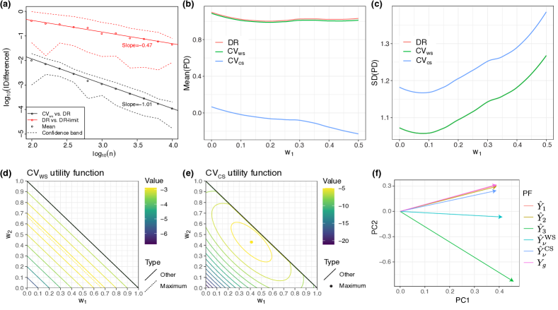
Figure 2: (a) $|\hat{U}^{\text{DR}}(w;\mathbf{1}_{K}/K)-\hat{U}^{\text{WS}}(w;\mathbf{1}_{K}/K)|$ (black) and $|\hat{U}^{\text{DR}}(w;\mathbf{1}_{K}/K)-\lim_{n\to\infty}\hat{U}^{\text{DR}}(w;\mathbf{1}_{K}/K)|$ (red) at $w=\mathbf{1}_{K}/K$ as a function of $n$. A 5-fold $\text{CV}_{\text{ws}}$ is used and we repeat the simulation for 40 times. Both X-axis and Y-axis are $\log_{10}$ transformed. The dashed lines indicate the upper and lower fifth percentile of the differences. The solid lines illustrate the linear approximation of log-transformed difference (black and red dots). The slopes approximate the rates of convergence of the differences when $n\to\infty$. (b-c) Mean and standard deviation of PDs for DR, $\text{CV}_{\text{ws}}$, $\text{CV}_{\text{cs}}$ stacking based on simulations. The simulation setting is described in Section 3.2.2. We plot the mean and standard deviation at 11 different $w$ where $w=(w_{1},(1-w_{1})/(K-1),\ldots,(1-w_{1})/(K-1))$ and $w_{1}$ varies from 0 to 0.5 with $0.05$ increment. For each value of $w$, 50 replicates are performed to calculate the mean and standard deviation. Note that in (c) the curves for DR and $\text{CV}_{\text{ws}}$ stacking overlap with each other. (d-f) Comparisons of $\text{CV}_{\text{ws}}$ and $\text{CV}_{\text{cs}}$ in generalist predictions (Example 3). We visualize the contour plots of $\hat{U}^{\text{WS}}(w;1/3\mathbf{1}_{3})$ (d) and $\hat{U}^{\text{CS}}(w;\mathbf{1}_{3}/3)$ (e). The solid lines are contour lines and the color indicates the function value of this contour. We use a dashed line and a dot to illustrate the maximizers of $\hat{U}^{\text{WS}}(w;\mathbf{1}_{3}/3)$ and $\hat{U}^{\text{CS}}(w;\mathbf{1}_{3}/3)$ respectively. (f) PCA of different PFs. We include three SPFs $\hat{Y}_{k}$, two stacked PFs $\hat{Y}^{\text{WS}}_{\nu}$ and $\hat{Y}^{\text{CS}}_{\nu}$ ($\nu=\mathbf{1}_{3}/3$), and the oracle PF $Y_{g}$.

$\text{CV}_{\text{cs}}$ can also be applied when $\mathcal{D}$ is not study-specific and with overlapping $D_{t}$ sets. We extend the definition of $\hat{U}^{\text{CS}}_{k}(w)$,

$$\hat{U}^{\text{CS}}_{k}(w)=\frac{1}{n_{k}}\sum_{i}u\left(\sum_{\ell,t}\mathbb{I}(k\notin s_{t})w_{\ell,t}\hat{Y}_{t}^{\ell}(x_{i,k}),y_{i,k}\right),$$

where $s_{t}=\{k:(i,k)\in D_{t}\text{ for some }i=1,\ldots,n_{k}\}$. Similar to the study-specific setting ($\mathcal{D}=\{D_{k}^{(s)};k=1,\ldots,K\}$), with exchangeable distributions $(P_{1},P_{2},\ldots)$, we have

$$\mathbb{E}\left[\hat{U}^{\text{CS}}_{k}(w)\mid\mathcal{D}_{-k}\right]=U_{g}(w^{(k)}),$$

where $w^{(k)}$ is equal to $w$ except for all elements $w_{\ell,t}$ such that $k\in s_{t}$, which are equal to zero. The $\hat{U}^{\text{CS}}_{k}(w)$ are combined into $\hat{U}^{\text{CS}}(w;\nu)$. Using the same Taylor expansion argument as in the previous paragraphs,

$$\sum_{k}\nu_{k}\mathbb{E}\left[\hat{U}^{\text{CS}}_{k}(w)\bigg{|}\mathcal{D}_{-k}\right]\approx U_{g}(\Gamma w),$$

where $\Gamma$ is a $KT\times KT$ diagonal matrix with the term corresponding to $w_{\ell,t}$ equal to $1-\sum_{k\in s_{t}}\nu_{k}$. Therefore the estimator of utility is

$$\hat{U}^{\text{CS}}(w;\nu)=\sum_{k}\frac{\nu_{k}}{n_{k}}\sum_{i=1}^{n_{k}}u\left(\sum_{\ell,t}\frac{\mathbb{I}(k\notin s_{t})}{1-\sum_{k\in s_{t}}\nu_{k}}w_{\ell,t}\hat{Y}_{t}^{\ell}(x_{i,k}),y_{i,k}\right).$$ (14)

An implicit assumption in (14) is that $(1-\sum_{k\in s_{t}}\nu_{k})>0$, that is, $D_{t}$ does not contain samples from all studies $k=1,\ldots,K$.

3.3 Penalization in specialist and generalist stacking

Adding penalties to a utility function estimate $\hat{U}(w)$ has been proposed for selecting weights $w$ in stacking (Breiman, 1996; LeBlanc and Tibshirani, 1996). Various forms of penalties can mirror a variety of relationships between the SPFs in $\hat{\mathcal{Y}}$. For example, group LASSO can be used when SPFs are organized into related groups.

In some cases, stacking without penalty on $w$ fails to incorporate information from other studies. We mention, for example, DR stacking PF $\hat{Y}^{\text{DR}}_{e_{k}}$ for specialist predictions with study-specific $\mathcal{D}$ and OLS regression ($L=1$), selects null weights on SPFs $\hat{Y}_{k^{\prime}}^{\ell}$ from studies $k^{\prime}\neq k$ (i.e., $w_{k^{\prime},\ell}=0$ if $k^{\prime}\neq k$). This is a limitation of the specialist PF $\hat{Y}^{\text{DR}}_{e_{k}}=\hat{Y}_{k}^{\ell}$ when study $k$ has small size $n_{k}$. A generalist PF is a good candidate for predictions in studies $k>K$ and similarly in studies $1,\ldots,K$ with small size. We discuss a penalization scheme to select $w$ for specialist predictions that shrinks the stacked PFs $\hat{Y}_{w}$ towards a generalist model.

We introduce the penalization using the utility function $\hat{U}^{\text{DR}}(w;e_{k})$. The same penalization can be applied to $\hat{U}^{\text{WS}}(w;e_{k})$. Let $\nu_{g}=\mathbf{1}_{K}/K$. The selection of specialist stacking weights is based on the optimization of

$$\hat{U}^{\text{DR}}_{\lambda}(w;e_{k})=\hat{U}^{\text{DR}}(w;e_{k})-\lambda\|w-\hat{w}^{\text{DR}}_{\nu_{g}}\|_{2}^{2},$$ (15)

where $\lambda>0$ is a tuning parameter, and $\hat{w}^{\text{DR}}_{\nu_{g}}$ denotes the generalist stacking weights. Let $\hat{w}^{\text{DR}}_{e_{k},\lambda}=\operatorname*{arg\,max}_{w\in W}\hat{U}^{\text{DR}}_{\lambda}(w;e_{k})$ and the associated PF be $\hat{Y}^{\text{DR}}_{e_{k},\lambda}$.

We use a leave-one-out cross-validation procedure to select $\lambda$. For sample $i=1,\ldots,n_{k}$ in study $k$, we generate $\hat{\mathcal{Y}}$ with sample $i$ excluded. We then calculate the prediction error of the resulting stacked PF with weights $\hat{w}^{\text{DR}}_{e_{k},\lambda}$ on sample $i$. This procedure is repeated for candidate values of $\lambda$.

Example 1, continued. We use the penalty introduced in (15) and evaluate the resulting PF $\hat{Y}^{\text{DR}}_{e_{k},\lambda}$ with the $\text{MSE}_{k}(\hat{w}^{\text{DR}}_{e_{k},\lambda})=\int_{(x,y)}(y-\hat{Y}^{\text{DR}}_{e_{k},\lambda}(x))^{2}dP_{k}(x,y).$ The parameters $\mu_{1}$ and $\mu_{2}$ are fixed. We have $\hat{Y}^{\text{DR}}_{e_{1}}=\bar{y}_{1}$, and, for any $\lambda>0$ (see Appendix for derivations),

$$\hat{Y}^{\text{DR}}_{e_{1},\lambda}=\frac{(\bar{y}_{1}-\bar{y}_{2})^{2}\bar{y}_{1}+2\lambda((\bar{y}_{1}+\bar{y}_{2})/2)}{(\bar{y}_{1}-\bar{y}_{2})^{2}+2\lambda}.$$

The penalized PF is a weighted average between the generalist PF $\hat{Y}^{\text{DR}}_{w,(1/2,1/2)}=(\bar{y}_{1}+\bar{y}_{2})/2$ and the specialist PF $\hat{Y}^{\text{DR}}_{w,e_{1}}=\bar{y}_{1}$. We consider the probability of $\text{MSE}_{1}(\hat{w}^{\text{DR}}_{e_{1}})\leq\text{MSE}_{1}(\hat{w}^{\text{DR}}_{e_{1},\lambda})$ for every $\lambda>0$:

$$\text{Pr}\left(\text{MSE}_{1}(\hat{w}^{\text{DR}}_{e_{1}})\leq\text{MSE}_{1}(\hat{w}^{\text{DR}}_{e_{1},\lambda}),\forall\lambda>0\right)=\text{Pr}(\mu_{1}\leq\bar{y}_{1}\leq\bar{y}_{2})+\text{Pr}(\mu_{1}\geq\bar{y}_{1}\geq\bar{y}_{2}).$$

We leverage the fact that $(\bar{y}_{1}-\bar{y}_{2},\bar{y}_{1}-\mu_{1})$ follows a bivariate normal distribution. When $\mu_{1}=\mu_{2}$, $\text{Pr}(\mu_{1}\leq\bar{y}_{1}\leq\bar{y}_{2})+\text{Pr}(\mu_{1}\geq\bar{y}_{1}\geq\bar{y}_{2})=1/2-\arcsin(1/\sqrt{1+n_{1}/n_{2}})/\pi$, which is an increasing function of $n_{1}/n_{2}$ and it converges to 0 when $n_{1}/n_{2}\to 0$. When $\mu_{1}\neq\mu_{2}$ and $n_{1}/n_{2}\approx 0$, the probability that penalty does not improve $\hat{Y}^{\text{DR}}_{w,e_{1}}$ is an increasing function of $|\mu_{1}-\mu_{2}|$ (study 2 is too different from study 1), and is below $0.5$.

Example 2, continued. We consider specialist predictions for $k=1$. We illustrate the effect of penalizing DR stacking, with $K=5$, $n_{1}=10$ and $n_{k}=100$ for $k=2,\ldots,5$. We set $\sigma_{\beta}=1$. In Figure 3 left panel, we compare the expected MSEs of three types of specialist PFs, i.e., $\hat{Y}^{\text{DR}}_{e_{1}},\hat{Y}^{\text{DR}}_{e_{1},\lambda}$ and $\hat{Y}^{\text{DR}}_{\nu_{g}}$, where $\nu_{g}=\mathbf{1}_{K}/K$, on new samples from study 1 when $\lambda$ changes from $10^{-3}$ to $10^{3}$ in a single simulation. In the figure as $\lambda$ increases from zero, the $\text{MSE}_{1}$ of $\hat{Y}^{\text{DR}}_{w,e_{k},\lambda}$ decreases. The $\text{MSE}_{1}$ is minimized at $\lambda\approx 2$ and when $\lambda$ increases beyond it, the $\text{MSE}_{1}$ increases. The selected $\lambda$ using the leave-one-out CV as described earlier is approximately $3.2$, which is in the region where penalization tends to improve DR stacking.

Based on expression (15), we describe a procedure to borrow information across a collection of small studies for generalist predictions.

1. For study $k=1,\ldots,K$, use $\hat{U}^{\text{DR}}(w;e_{k})$ to generate a specialist PF $\hat{Y}^{\text{DR}}_{e_{k}}$.

2. Average $\hat{Y}^{\text{DR}}_{e_{k}}$, $k=1,\ldots,K$ to obtain a PF $\hat{Y}_{g,\text{av}}=\sum_{k}\hat{Y}^{\text{DR}}_{e_{k}}/K$. The stacking weights associated with $\hat{Y}_{g,\text{av}}$ is $\hat{w}_{g,\text{av}}=\sum_{k}\hat{w}^{\text{DR}}_{e_{k}}/K$. The subindex “av” refers to the averaging of specialist models.

3. For study $k=1,\ldots,K$, use $\hat{U}^{\text{DR}}_{\lambda}(w;e_{k})$ with $\hat{w}^{\text{DR}}_{\nu_{g}}=\hat{w}_{g,\text{av}}$ to obtain an updated specialist PF $\hat{Y}^{\text{DR}}_{e_{k},\lambda}$. $\lambda$ is selected separately for each $k$ with standard leave-one-out CV.

4. Repeat Step 2-3 with input $\hat{Y}^{\text{DR}}_{e_{k},\lambda}$ instead of $\hat{Y}^{\text{DR}}_{e_{k}}$ until the PF $\hat{Y}_{g,\text{av}}$ converges.

We apply the above approach to train $\hat{Y}^{\text{DR}}_{g,\text{av}}$ in Example 2. We assume that $K=20$, $n_{k}=15$ for $k=1,\ldots,10$, and $n_{k}=100$ for $k=11,\ldots,20$. We set $\sigma_{\beta}=1$, $p=10$ and $\beta_{0}=\mathbf{1}_{p}$. In Figure 3 right panel, we illustrate the generalist prediction accuracy $\text{MSE}_{0}(\hat{Y}^{\text{DR}}_{g,\text{av}})$ as the number of iterations increases. After three iterations, $\text{MSE}_{0}(\hat{Y}^{\text{DR}}_{g,\text{av}})$ is substantially smaller than the initial value of $\hat{Y}^{\text{DR}}_{g,\text{av}}$, $\sum_{k}\hat{Y}^{\text{DR}}_{e_{k}}/K$. The accuracy stabilizes after four iterations and is larger than the $\text{MSE}_{0}$ of the average of the true PFs of study $k=1,\ldots,K$, $\sum_{k}Y_{e_{k}}/K$, where $Y_{e_{k}}(x)=\beta_{k}^{\intercal}x$.

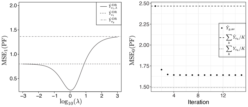
Figure 3: (Left) Effect of penalization on specialist prediction. $\lambda$ controls the strength of the penalization. Larger $\lambda$ shrinks the specialist predictions more towards generalist predictions. The two types of dashed lines indicate the expected MSE when $\lambda=0$ ($\hat{Y}^{\text{DR}}_{e_{1}}$) and $\lambda\to\infty$ ($\hat{Y}^{\text{DR}}_{\nu_{g}}$). The plot is based on a single simulation replicate. The X-axis is $\log_{10}$ transformed. (Right) Generalist prediction accuracy of $\hat{Y}_{g,\text{av}}$ as the number of iterations increases. The two dashed lines indicate $\text{MSE}_{0}$ of the average of DR specialist PFs without penalization $\hat{Y}^{\text{DR}}_{e_{k}}$ and of true PFs $Y_{e_{k}}(x)=\beta_{k}^{\intercal}x$. Both panels are based on simulations described in Section 3.3.

4 Properties of generalist prediction models

In consideration of the asymptotic similarity of $\hat{Y}^{\text{DR}}_{w,\nu}$ and $\hat{Y}^{\text{WS}}_{w,\nu}$, we focus on the comparison between $\text{CV}_{\text{cs}}$ and DR stacking. We suppress the subscript $\nu$ in this section and assume $\nu=\mathbf{1}_{K}/K$. We will assume that the data collection is generated from a hierarchical model, and that $\mathcal{D}$ is study-specific.

We discuss two properties. First, the expected MSE of the generalist PFs in future $k>K$ studies with $\hat{w}^{\text{DR}}$ and $\hat{w}^{\text{CS}}$ is close to the MSE of an asymptotic oracle PF when $n_{k}$ and $K$ are large. The discrepancy between the MSEs will be bounded by a monotone function of $K$ and $(\min_{k}n_{k})$. Second, we investigate in a special case the relative performance of DR stacking and $\text{CV}_{\text{cs}}$ in generalist predictions.

We extend the joint hierarchical model in Example 2 to allow for arbitrary regression functions $\mathbb{E}(y_{i,k}|x_{i,k})$:

$$y_{i,k}=f_{k}(x_{i,k})+\epsilon_{i,k},$$ (16)

$$f_{k}\overset{iid}{\sim}F_{f},~{}x_{i,k}\buildrel iid\over{\sim}F_{X},$$

for $i=1,\ldots,n_{k}$ and $k=1,2,\ldots$. Here $f_{k}:\mathbb{R}^{p}\to\mathbb{R}$, $k\geq 1$, are random functions. The mean of $F_{f}$ is indicated as $f_{0}=\int fdF_{f}$. The vectors $x_{i,k}\in\mathcal{X}$ have the same distribution $F_{X}$ with finite second moments across datasets, and the noise terms $\epsilon_{i,k}$ are independent with mean zero and variance $\sigma^{2}$.

Our Proposition 2 will assume:

1. There exists an $M_{1}<\infty$ such that a.e. (i.e., with probability 1) for any $k>0$ and $\ell\leq L$,

   $$\sup_{x\in\mathcal{X}}|f_{k}(x)|\leq M_{1},~{}\sup_{x\in\mathcal{X}}|\hat{Y}_{k}^{\ell}(x)|\leq M_{1},\text{ and,}~{}|y_{i,k}|\leq M_{1}.$$

   The first inequality has probability 1 with respect to $F_{f}$, whereas for the second and third inequalities we consider the distribution of $\mathcal{S}$. These assumptions are not particularly restrictive. For example, if $\mathcal{X}$ is a compact set and the outcomes $Y$ are bounded, the SPFs trained with a penalized linear regression model, e.g. a LASSO regression, or with tree-based regression models satisfy the assumption.

2. There exist constants $M_{2}<\infty$, $p_{\ell}>0$ and random functions $Y_{k}^{\ell}$ for $k=1,\ldots,K$, $\ell=1,\ldots,L$, such that $\sup_{x\in\mathcal{X}}|Y_{k}^{\ell}(x)|\leq M_{1}~{}a.e.,$ and for every large enough $n_{k}$, $k=1,\ldots,K$,

   $$\mathbb{E}\left[\int_{x}n_{k}^{2p_{\ell}}\left(\hat{Y}_{k}^{\ell}(x)-Y_{k}^{\ell}(x)\right)^{2}dF_{X}(x)\right]\leq M_{2},$$

   where the expectation is with respect to the distribution of $\mathcal{S}$ and $Y_{k}^{\ell}$ is the limit of $\hat{Y}_{k}^{\ell}$. For example, if $\hat{Y}_{k}^{\ell}$ is an OLS regression function and $\|\mathbb{E}((X_{k}^{\intercal}X_{k})^{-1})\|_{F}=O(1/n_{k})$, where $\|\cdot\|_{F}$ is the Frobenius norm, then $Y_{k}^{\ell}(x)=(\lim\hat{\beta}_{k})^{\intercal}x$ and $p_{\ell}\leq 1/2$ satisfy the above inequality.

Let $X_{k}=(x_{1,k},\ldots,x_{n_{k},k})^{\intercal}$, $Y_{k}=(y_{1,k},\ldots,y_{n_{k},k})^{\intercal}$, and $\hat{Y}_{k^{\prime}}^{\ell}(X_{k})=(\hat{Y}^{\ell}_{k^{\prime}}(x_{i,k});i\leq n_{k})^{\intercal}$. We have

$$\begin{gathered}\hat{U}^{\text{DR}}(w;K^{-1}\mathbf{1}_{K})=w^{\intercal}\hat{\Sigma}^{\text{DR}}w-2(\hat{b}^{\text{DR}})^{\intercal}w+K^{-1}\sum_{k}n^{-1}_{k}\sum_{i}y_{i,k}^{2},\\ \hat{U}^{\text{CS}}(w;K^{-1}\mathbf{1}_{K})=w^{\intercal}\hat{\Sigma}^{\text{CS}}w-2(\hat{b}^{\text{CS}})^{\intercal}w+K^{-1}\sum_{k}n^{-1}_{k}\sum_{i}y_{i,k}^{2},\end{gathered}$$ (17)

where the $\hat{\Sigma}^{\text{DR}},\hat{\Sigma}^{\text{CS}},\hat{b}^{\text{DR}},$ and $\hat{b}^{\text{CS}}$ components are

$$\hat{\Sigma}^{\text{DR}}_{k,k^{\prime};\ell,\ell^{\prime}}=\sum_{i=1}^{K}\frac{\left(\hat{Y}_{k}^{\ell}(X_{i})\right)^{\intercal}\hat{Y}_{k^{\prime}}^{\ell^{\prime}}(X_{i})}{n_{i}K},~{}~{}\hat{b}^{\text{DR}}_{k;\ell}=\sum_{i=1}^{K}\frac{\left(\hat{Y}_{k}^{\ell}(X_{i})\right)^{\intercal}Y_{i}}{n_{i}K},$$

$$\hat{\Sigma}^{\text{CS}}_{k,k^{\prime};\ell,\ell^{\prime}}=\sum_{i\neq k,i\neq k^{\prime}}\frac{K\left(\hat{Y}_{k}^{\ell}(X_{i})\right)^{\intercal}\hat{Y}_{k^{\prime}}^{\ell^{\prime}}(X_{i})}{n_{i}(K-1)^{2}},~{}~{}\hat{b}_{k;\ell}^{\text{CS}}=\sum_{i\neq k}\frac{\left(\hat{Y}_{k}^{\ell}(X_{i})\right)^{\intercal}Y_{i}}{n_{i}(K-1)}.$$

Here $\hat{\Sigma}^{\text{DR}}$ and $\hat{\Sigma}^{\text{CS}}$ are $KL\times KL$ matrices, and $w$, $\hat{b}^{\text{DR}}$ and $\hat{b}^{\text{CS}}$ are $KL$-dimensional vectors. $\hat{\Sigma}_{k,k^{\prime};\ell,\ell^{\prime}}$ is the element corresponding to $w_{k,\ell}$ and $w_{k^{\prime},\ell^{\prime}}$ while $\hat{b}_{k;\ell}$ corresponds to $w_{k,\ell}$.

We define the limiting oracle generalist stacking weights $w_{g}^{0}$ based on the limits $Y_{k}^{\ell}$ of $\hat{Y}_{k}^{\ell}$, $k=1,\ldots,K,\ell=1,\ldots,L$:

$$w_{g}^{0}=\operatorname*{arg\,max}_{w\in W}\int_{x,y}u(Y_{w}(x),y)dP_{0}(x,y),$$

where $Y_{w}=\sum_{\ell,t}w_{\ell,t}Y_{t}^{\ell}$ and $P_{0}$ (defined in Section 2.2) is the average joint distribution of $(X,Y)$ across studies $k\geq 1$. The generalist prediction accuracy of $Y_{w}$ is

$$\psi(w)=\int_{x,y}(y-Y_{w}(x))^{2}dP_{0}(x,y)=w^{\intercal}\Sigma w-2b^{\intercal}w+\int_{y}y^{2}dP_{0}(y),$$

where $\Sigma_{k,k^{\prime};\ell,\ell^{\prime}}=\int_{x}Y_{k}^{\ell}(x)Y_{k^{\prime}}^{\ell^{\prime}}(x)dF_{X}(x)$ and $b_{k;\ell}=\int_{x,y}yY_{k}^{\ell}(x)dP_{0}(x,y)$. In Proposition 2 we compare $\hat{Y}^{\text{DR}}_{w}$ and $\hat{Y}^{\text{CS}}_{w}$ to the asymptotic oracle PF, using the metrics $\mathbb{E}(\psi(\hat{w}^{\text{DR}})-\psi(w_{g}^{0}))$ and $\mathbb{E}(\psi(\hat{w}^{\text{CS}})-\psi(w_{g}^{0}))$.

Proposition 2.

Let $K\geq 2$ and $w\in\Delta_{KL-1}$. Consider $K$ available datasets and future $k>K$ studies from model (16). If (A1) and (A2) hold, then

$$\mathbb{E}\left(\psi(\hat{w}^{\text{DR}})-\psi(w_{g}^{0})\right)\leq C_{0}\sqrt{\log(KL)}K^{-1/2}+C_{1}(\min_{k}n_{k})^{-\min_{\ell}p_{\ell}},$$

and,

$$\mathbb{E}\left(\psi(\hat{w}^{\text{CS}})-\psi(w_{g}^{0})\right)\leq C_{0}^{\prime}\sqrt{\log(KL)}K^{-1/2}+C_{1}^{\prime}(\min_{k}n_{k})^{-\min_{\ell}p_{\ell}},$$

where the expectations are taken over the joint distribution of the data $\mathcal{S}$. $C_{0}$, $C_{0}^{\prime}$, $C_{1}$ and $C_{1}^{\prime}$ are constants, independent of $K$ and $n_{k}$.

The above proposition shows that if we have enough studies and samples in each study, then the estimated generalist PFs $\hat{Y}^{\text{DR}}$ and $\hat{Y}^{\text{CS}}$ have similar accuracy compared to $Y_{w_{g}^{0}}$.

We then compare $\psi(\hat{w}^{\text{DR}})$ and $\psi(\hat{w}^{\text{CS}})$ in a special case and prove a proposition on the relative accuracy levels of these two methods. Consider again the model in Example 2 and set $n_{k}=n$. Let $\hat{\beta}_{k}$ be the OLS estimate of $\beta_{k}$, and $\hat{Y}_{k}(x)=\hat{\beta}_{k}^{\intercal}x$, denote $\bm{\beta}=(\beta_{1},\ldots,\beta_{K})$ and $\hat{\bm{\beta}}=(\hat{\beta}_{1},\ldots,\hat{\beta}_{K})$. We have $\Sigma_{g;k,k^{\prime}}=\hat{\beta}_{k}^{\intercal}\hat{\beta}_{k^{\prime}}$, $b_{g;k}=\hat{\beta}_{k}^{\intercal}\beta_{0}$ and

$$\begin{gathered}\hat{\Sigma}^{\text{DR}}_{k,k^{\prime}}=(nK)^{-1}\sum_{s}\hat{\beta}_{k}^{\intercal}X_{s}^{\intercal}X_{s}\hat{\beta}_{k^{\prime}},~{}\hat{b}^{\text{DR}}_{k}=(nK)^{-1}\sum_{s}\hat{\beta}_{k}^{\intercal}X_{s}^{\intercal}Y_{s},\\ \hat{\Sigma}_{k,k^{\prime}}^{\text{CS}}=\frac{K}{n(K-1)^{2}}\sum_{\begin{subarray}{c}s\neq k\\ s\neq k^{\prime}\end{subarray}}\hat{\beta}_{k}^{\intercal}X_{s}^{\intercal}X_{s}\hat{\beta}_{k^{\prime}},~{}\hat{b}_{k}^{\text{CS}}=\left(n(K-1)\right)^{-1}\sum_{s\neq k}\hat{\beta}_{k}^{\intercal}X_{s}^{\intercal}Y_{s}.\end{gathered}$$ (18)

We consider the expected PDs.

$$\mathbb{E}\left(d\left(\hat{U}^{\text{DR}}(w;K^{-1}\mathbf{1}_{K}),U_{g}^{0}(w)\right)\right)=\frac{p(p+1)\sigma^{2}}{Kn(n-p-1)}\|w\|_{2}^{2}+\frac{2(p\sigma_{\beta}^{2}+p\sigma^{2}/n)}{K}w^{\intercal}\mathbf{1}_{K}$$

$$\mathbb{E}\left(d\left(\hat{U}^{\text{CS}}(w;K^{-1}\mathbf{1}_{K}),U_{g}^{0}(w)\right)\right)=\frac{\|\beta_{0}\|_{2}^{2}}{(K-1)^{2}}\sum_{k\neq k^{\prime}}w_{k}w_{k^{\prime}}-\frac{\|\beta_{0}\|_{2}^{2}+p\sigma_{\beta}^{2}+p\sigma^{2}/(n-p-1)}{K-1}\|w\|_{2}^{2}.$$

$\mathbb{E}(d(\hat{U}^{\text{DR}}(w;K^{-1}\mathbf{1}_{K}),U_{g}^{0}(w)))\geq 0$ and $\mathbb{E}(d(\hat{U}^{\text{CS}}(w;K^{-1}\mathbf{1}_{K}),U_{g}^{0}(w)))\leq 0$ for any $w\in\Delta_{K-1}$. When $\|\beta_{0}\|_{2}=o(\sigma_{\beta})$, the absolute bias of DR stacking is uniformly larger than $\text{CV}_{\text{cs}}$. If $\sigma_{\beta}=o(\|\beta_{0}\|_{2})$, the absolute bias of DR stacking is uniformly smaller than $\text{CV}_{\text{cs}}$ (see Appendix for derivations). Although smaller absolute bias does not imply better generalist prediction accuracy, the relative accuracy levels of DR stacking to $\text{CV}_{\text{cs}}$, as measured by $\mathbb{E}(\psi(\hat{w}^{\text{DR}})-\psi(\hat{w}^{\text{CS}})$, follows a similar trend as $\sigma_{\beta}$ changes. In Figure 4, we use simulated data to illustrate the trend. We set $p=10$, $\beta_{0}=\mathbf{1}_{p}$ and $n=200$, and examine two scenarios $K=2$ and $K=9$. $\mathbb{E}(\psi(w))$ is calculated with 1,000 replicates. As illustrated in the figures, when $\sigma_{\beta}$ is small, $\text{CV}_{\text{cs}}$ has lower generalist prediction accuracy than DR stacking ($\mathbb{E}(\psi(\hat{w}^{\text{DR}})-\psi(\hat{w}^{\text{CS}}))<0$). When $\sigma_{\beta}$ is large, $\text{CV}_{\text{cs}}$ outperforms DR stacking.

Figure 4: Comparison of DR stacking and $\text{CV}_{\text{cs}}$ when $K=2$ (left) and $K=9$ (right). The plots illustrate the differences $\mathbb{E}(\psi(\hat{w}^{\text{DR}})-\psi(\hat{w}^{\text{CS}}))$ (solid lines) and $\mathbb{E}(\psi(\hat{w}^{\text{DR}})-\psi(w_{g}^{0}))$ (dahsed lines). We set $p=10$, $\beta_{0}=\mathbf{1}_{K}$, $n=200$, and vary $\sigma_{\beta}$. The expected values are calculated with 1,000 replicates.

In Proposition 3, we formally characterize the relationship between $\mathbb{E}(\psi(\hat{w}^{\text{DR}})-\psi(\hat{w}^{\text{CS}}))$ and $\sigma_{\beta}$ in the setting where $n_{k}\to\infty$ and $K>2$ is fixed.

Proposition 3.

Consider the model in Example 2 with an OLS learner ($L=1$). Assume $n_{k}\to\infty$, $K>2$ and $W=\mathbb{R}^{K}$. If $\beta_{0}=\mathbf{0}$, then $\mathbb{E}(\psi(\hat{w}^{\text{DR}})-\psi(\hat{w}^{\text{CS}}))>0$ for every $\sigma_{\beta}>0$. If $\beta_{0}\neq\mathbf{0}$, $\mathbb{E}(\psi(\hat{w}^{\text{DR}})-\psi(\hat{w}^{\text{CS}}))\to\infty$ when $\sigma_{\beta}\to\infty$ and $\mathbb{E}(\psi(\hat{w}^{\text{DR}})-\psi(\hat{w}^{\text{CS}}))\uparrow 0$ when $\sigma_{\beta}\to 0$.

5 Simulation studies

We first illustrate with simulations the penalization approach in Section 3.3. We then investigate empirically whether the error bounds in Proposition 2 are tight, and how the difference $\mathbb{E}(\psi(\hat{w}^{\text{DR}}))-\mathbb{E}(\psi(\hat{w}^{\text{CS}}))$ changes as $K$ and inter-study heterogeneity $\sigma_{\beta}$ vary.

We simulate the data using the generative model in Example 2 and specialize predictions to study 1. We set $p=10$, $K=5$, $n_{k}=100$ for $k=2,\ldots,5$ and $n_{1}$ varying from $15$ to $45$. $\beta_{0}=\mathbf{1}_{10}$, $\sigma_{\beta}=1$, $\sigma=5$, $\mathcal{D}$ is study-specific and the only learner ($L=1$) is OLS regression. We compare $\hat{Y}^{\text{DR}}_{w,e_{1},\lambda}$ to $\hat{Y}^{\text{DR}}_{w,e_{1}}$ and examine whether the penalty we introduce in (15) improves accuracy. We also include in the comparison the the generalist PF $\hat{Y}^{\text{DR}}_{w,\mathbf{1}_{K}/K}$. In Figure 5(a), we illustrate the $\text{MSE}_{1}$ of these three PFs.

We can see that when $n_{1}$ is small ($n_{1}<30$), $\hat{Y}^{\text{DR}}_{w,e_{1}}$ has the worst performance. $\hat{Y}^{\text{DR}}_{w,\mathbf{1}_{K}/K}$ as expected has stable $\text{MSE}_{1}$ as $n_{1}$ increases from 15 to 50 and outperforms $\hat{Y}^{\text{DR}}_{w,e_{1}}$ when $n_{1}<35$. When $n_{1}\geq 40$ the specialist PF has smaller $\text{MSE}_{1}$ than the generalist PF. The penalized specialist PF $\hat{Y}^{\text{DR}}_{w,e_{1},\lambda}$ has the lowest $\text{MSE}_{1}$.

We then illustrate the difference $\mathbb{E}\left(\psi(\hat{w}^{\text{DR}})-\psi(w_{g}^{0})\right)$ considered in Proposition 2 with a numeric example and compare the actual difference to the analytic upper bound as $n_{k}$ and $K$ change. We use a simulation scenario similar to the previous setting with each component of $\beta_{k}$ uniformly distributed in $[0,1]$. Each component of $x_{i,k}$ is uniform in $[-1,1]$ and $\epsilon_{i,k}$ is uniform in $[-1,1]$. We set $n_{k}=n$ for all $k$ and approximate with Monte Carlo simulations $\mathbb{E}\left(\psi(\hat{w}^{\text{DR}})-\psi(w_{g}^{0})\right)$ for $n=100,200,400$ as $K$ increases from $20$ to $50$ and for $K=5,15,20$ as $n$ increases from $20$ to $100$. We use the constraint $w\in\Delta_{K-1}$. The results are derived from 1000 simulation replicates and shown in Figure 5(b-c). The difference $\mathbb{E}(\psi(\hat{w}^{\text{DR}})-\psi(w_{g}^{0}))$ is approximately a linear function of $\sqrt{\log{K}/K}$ (Fig. 5(b)) and $n^{-1/2}$ (Fig. 5(c)). The results for $\mathbb{E}(\psi(\hat{w}^{\text{CS}})-\psi(w_{g}^{0}))$ are similar (see Appendix Fig. E.1).

Finally, we perform a simulation analysis strictly related to the main results in Proposition 3. This numerical analysis identifies regions where $\mathbb{E}(\psi(\hat{w}^{\text{DR}})-\psi(\hat{w}^{\text{CS}}))>0$. We use the data generating model in Example 2. We fix $\beta_{0}=\mathbf{1}_{10}$ and vary $\sigma_{\beta}$ between 0 and 4 and the number of studies $K$ from 3 to 50. We then approximate $\mathbb{E}(\psi(\hat{w}^{\text{DR}}))-\mathbb{E}(\psi(\hat{w}^{\text{CS}}))$ with Monte Carlo simulations (Fig. 5(d)). In this figure the regions of $K$ and $\sigma_{\beta}$ in which $\mathbb{E}(\psi(\hat{w}^{\text{DR}}))-\mathbb{E}(\psi(\hat{w}^{\text{CS}}))<0$ are in blue. Otherwise, the regions are in red. We can see that when $\sigma_{\beta}$ is large, it is useful to switch from DR stacking to $\text{CV}_{\text{cs}}$ for generalist predictions.

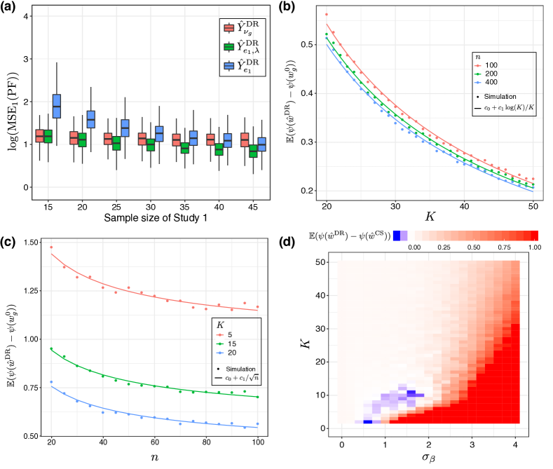
Figure 5: (a) Specialist prediction accuracy of $\hat{Y}^{\text{DR}}_{\nu_{g}}$, $\hat{Y}^{\text{DR}}_{e_{1}}$ and $\hat{Y}^{\text{DR}}_{e_{1},\lambda}$ on study 1 as measured by $\text{MSE}_{1}$. The boxplots illustrate the variability of accuracy over 50 simulation replicates. $\lambda$ is selected using the leave-one-out cross-validation introduced in Section 3.3. The data are generated using the model in (9). $K=5$ studies are generated with $n_{2}=\ldots=n_{5}=100$ and $n_{1}$ varying from 15 to 45. The inter-study heterogeneity $\sigma_{\beta}=1$ is much smaller than the within-study varability $\sigma=5$. Y-axis is log transformed. (b-c) $\mathbb{E}(\psi(\hat{w}^{\text{DR}})-\psi(w_{g}^{0}))$ as a function of $K$ and $n$. Dots represent results from the Monte Carlo simulation. Lines illustrate the fitted functions $c_{0}+c_{1}\log(K)/K$ (b) and $c_{0}+c_{1}/\sqrt{n}$ (c) to the Monte Carlo results. (d) Comparison of generalist prediciton accuracy of DR stacking and $\text{CV}_{\text{cs}}$ as measured by $\mathbb{E}(\psi(\hat{w}^{\text{DR}})-\psi(\hat{w}^{\text{CS}}))$.

6 Application

We develop generalist PFs based on an environmental health dataset. It contains annual mortality rates for the period 2000 to 2016 across 31,337 unique zip codes in the entire U.S. The annual average exposure to PM_2.5 is available for each zip code. In addition to the measurement of PM_2.5 and the annual mortality rate, we have zip code-level baseline demographic covariates, which include percentage of ever smokers, percentage of black population, median household income, median value of housing, percentage of the population below the poverty level, percentage of the population with education below high school, percentage of owner-occupied housing units, and population density.

We define the generalist prediction task as the prediction of zip code-level annual mortality rates from 2000 to 2016 in a region (e.g. State) based on exposure to PM_2.5 during the year and zip code-level demographic covariates. In other words, zip codes within a region constitute a study $k$. We also include year as a covariate to capture the temporal trends of mortality rate. We consider two levels of regions: state and county. For generalist predictions in the state-level, we randomly select 10 states to train an ensemble of state-specific $k=1,\ldots,10$ PFs with random forest, and use DR stacking and $\text{CV}_{\text{cs}}$ to combine them and predict mortality in 2000-2016 in the remaining 39 regions. Each state contains on average 980 unique zip codes and 13,936 zip code by year records. The metric we use to evaluate the accuracy of the stacked PF is the average RMSE across all testing regions and years. We repeat this procedure 20 times. The county-level analysis is performed by restricting the data collection only to the state of California and zip codes belong to the same county constitute study $k$. For this county-level dataset, we combine 10 county-specific PFs and validate the stacked PFs using the remaining 47 states. Each county contains on average 23 unique zip codes and 657 zip code by year records. The results are shown in Figure 6.

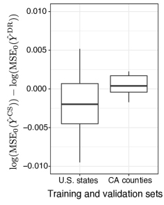
Figure 6: Comparisons of DR stacking and $\text{CV}_{\text{cs}}$ in generalist predictions of mortality. Each boxplot illustrates the accuracy of the two stacking methods over 20 simulation replicates, evaluated with average RMSE across all validation regions and years. In each replicate, we randomly select 10 regions to train SPFs in the ensemble and evaluate the stacked PF on the remaining regions (39 for state-specific SPFs and 47 for county-specific SPFs).

In the first case, when we combine state-specific PFs with considerable heterogeneity, the performance of $\text{CV}_{\text{cs}}$ is slightly better compared to DR stacking. In constrast, when we restrict the data collection to the state of California and combine county-level models, with reduced heterogeneity, DR stacking has a smaller mean RMSE than $\text{CV}_{\text{cs}}$. We also characterize between-study heterogeneity in the national dataset and the California dataset with variance of the predicted values from the 10 PFs on a sample with all covariates fixed at the national means. Across the 20 replicates, the mean of the standard deviation for the state-specific PFs is 0.017 and 0.0029 for the county-specific PFs. This result is aligned with Proposition 3, which indicates for a fixed $K$, $\text{CV}_{\text{cs}}$ can outperform DR when the inter-study heterogeneity is large.

7 Discussion

We studied a multi-study ensemble learning framework based on stacking for generalist and specialist predictions. We compared NDR ($\text{CV}_{\text{ws}}$ and $\text{CV}_{\text{cs}}$) and DR methods for the selection of stacking weights of SPFs in the ensemble. We discussed oracle properties of the generalist PFs and provide a condition under which $\text{CV}_{\text{cs}}$ can outperform DR stacking in a linear regression setting. We also considered a penalization scheme to address difficulties in generalist and specialist predictions when some studies have small size. We illustrated these theoretical developments with simulations and applied our approach to predict mortality from environmental factors based on multi-state and multi-county datasets.

We illustrated in examples that DR stacking is nearly identical to $\text{CV}_{\text{ws}}$ for generalist predictions while $\text{CV}_{\text{cs}}$ is substantially different from both of them. We showed that the penalization scheme we introduced for generalist and specialist predictions are beneficial when a subset of the $K$ studies are of small size. We examined the differences $\mathbb{E}(\psi(\hat{w}^{\text{DR}})-\psi(w_{g}^{0}))$ and $\mathbb{E}(\psi(\hat{w}^{\text{CS}})-\psi(w_{g}^{0}))$ with Monte Carlo simulations and confirmed under the simulation setting, they can be approximated by the functions of $K$ and $n$ discussed in Proposition 2. We also confirmed with both numerical experiments and analytical approaches that in the setting of Example 2, $\text{CV}_{\text{cs}}$ outperforms DR stacking ($\mathbb{E}(\psi(\hat{w}^{\text{DR}})-\psi(\hat{w}^{\text{CS}}))>0$) when $\sigma_{\beta}$ is large. Finally, we illustrated again through the application that $\text{CV}_{\text{cs}}$ tends to outperform DR stacking in generalist predictions when the heterogeneity of $E(Y|X)$ across studies is high.

Appendix A Derivations in Example 1 and 2

Example 1, DR stacking. Since $w\in\Delta_{1}$, the expected generalist utility is $U_{g}(w)=-(w_{1}\bar{y}_{1}+w_{2}\bar{y}_{2})^{2}-2=-(w_{1}(\bar{y}_{1}-\bar{y}_{2})+\bar{y}_{2})^{2}-2$, $w\in[0,1]$. If $\bar{y}_{1}=\bar{y}_{2}$, any $w\in\Delta_{1}$ is a maximizer of $U_{g}(w)$. If $\bar{y}_{1}\neq\bar{y}_{2}$ and $\bar{y}_{2}/(\bar{y}_{1}-\bar{y}_{2})\in[0,1]$, $U_{g}(w)$ is maximized at $w_{g}=(\bar{y}_{2}/(\bar{y}_{2}-\bar{y}_{1}),\bar{y}_{1}/(\bar{y}_{1}-\bar{y}_{2}))$. Note $\bar{y}_{2}/(\bar{y}_{2}-\bar{y}_{1})\in[0,1]$ if and only if $\bar{y}_{1}\cdot\bar{y}_{2}\leq 0$, in which case $\bar{y}_{2}/(\bar{y}_{2}-\bar{y}_{1})=|\bar{y}_{2}|/(|\bar{y}_{1}|+|\bar{y}_{2}|)$. If $\bar{y}_{2}/(\bar{y}_{2}-\bar{y}_{1})<0$, that is, $\bar{y}_{1}\cdot\bar{y}_{2}>0$ and $|\bar{y}_{1}|>|\bar{y}_{2}|$, $w_{g}=(0,1)$. If $\bar{y}_{1}\cdot\bar{y}_{2}>0$ and $|\bar{y}_{1}|<|\bar{y}_{2}|$, $\bar{y}_{2}/(\bar{y}_{2}-\bar{y}_{1})>1$ and $w_{g}=(1,0)$.

The estimated generalist utility based on DR stacking is

$$\hat{U}^{\text{DR}}(w;\nu)=-(w_{1}\bar{y}_{1}+w_{2}\bar{y}_{2})^{2}+2(\nu_{1}\bar{y}_{1}+\nu_{2}\bar{y}_{2})(w_{1}\bar{y}_{1}+w_{2}\bar{y}_{2})-\nu_{1}\overline{y_{1}^{2}}-\nu_{2}\overline{y_{2}^{2}},$$

and it follows that $\hat{w}^{\text{DR}}_{\nu}=\nu$ and $d(\hat{U}^{\text{DR}}(w;\nu),U_{g}(w))=2(\nu_{1}\bar{y}_{1}+\nu_{2}\bar{y}_{2})(w_{1}\bar{y}_{1}+w_{2}\bar{y}_{2})$. We note that $\bar{y}_{1}$ and $\bar{y}_{2}$ are independent $N(0,\sigma^{2}+1/n)$. Therefore when $\nu=(1/2,1/2)$,

$$\mathbb{E}\left(d(\hat{U}^{\text{DR}}(w;\nu),U_{g}(w))\right) =w_{1}\mathbb{E}(\bar{y}_{1}^{2})+w_{2}\mathbb{E}(\bar{y}_{2}^{2})=\sigma^{2}+1/n,$$

$$\mathbb{E}\left(d(\hat{U}^{\text{DR}}(w;\nu),U_{g}(w))^{2}\right) =w_{1}^{2}\mathbb{E}(\bar{y}_{1}^{4})+w_{2}^{2}\mathbb{E}(\bar{y}_{2}^{4})+(1+2w_{1}w_{2})\mathbb{E}(\bar{y}_{1}^{2}\bar{y}_{2}^{2})$$

$$= (3w_{1}^{2}+3w_{2}^{2}+2w_{1}w_{2}+1)(\sigma^{2}+1/n)^{2}.$$

Since $w\in\Delta_{1}$, we have $\text{var}(d(\hat{U}^{\text{DR}}(w;\nu),U_{g}(w)))=(2w_{1}^{2}+2w_{2}^{2}+1)(\sigma^{2}+1/n)^{2}$.

The expected specialist utility for $w\in\Delta_{1}$ is

$$U_{s}(w;1)=-w_{1}^{2}(\bar{y}_{1}-\bar{y}_{2})^{2}-2w_{1}(\bar{y}_{1}-\bar{y}_{2})(\bar{y}_{2}-\mu_{1})+2\mu_{1}\bar{y}_{2}-\mu_{1}^{2}-\bar{y}_{2}^{2}-1,~{}w_{1}\in[0,1].$$

If $\bar{y}_{1}=\bar{y}_{2}$, any $w\in\Delta_{1}$ is a maximizer of $U_{s}(w;1)$. If $\bar{y}_{1}\neq\bar{y}_{2}$ and $(\mu_{1}-\bar{y}_{2})/(\bar{y}_{1}-\bar{y}_{2})\in[0,1]$, $w_{s;1}^{(1)}=(\mu_{1}-\bar{y}_{2})/(\bar{y}_{1}-\bar{y}_{2})$. If $(\mu_{1}-\bar{y}_{2})/(\bar{y}_{1}-\bar{y}_{2})<0$, $w_{s;1}^{(1)}=0$ and $w_{s;1}^{(1)}=1$ if $(\mu_{1}-\bar{y}_{2})/(\bar{y}_{1}-\bar{y}_{2})>1$.

The estimated specialist utility from DR stacking is

$$\hat{U}^{\text{DR}}(w;e_{1})=-(w_{1}\bar{y}_{1}+w_{2}\bar{y}_{2})^{2}+2\bar{y}_{1}(w_{1}\bar{y}_{1}+w_{2}\bar{y}_{2})-\overline{y_{1}^{2}}.$$

Clearly the maximizer of $\hat{U}^{\text{DR}}(w;e_{1})$ is $\hat{w}^{\text{DR}}_{e_{1}}=(1,0)$ and $d(\hat{U}^{\text{DR}}(w;e_{1}),U_{s}(w;1))=2(\bar{y}_{1}-\mu_{1})(w_{1}\bar{y}_{1}+w_{2}\bar{y}_{2}).$ Although $\bar{y}_{1}$ and $\bar{y}_{2}$ are iid $N(0,\sigma^{2}+1/n)$, $\bar{y}_{1}$ and $\mu_{1}$ are not independent by noting that $\bar{y}_{1}=\mu_{1}+\epsilon$ where $\epsilon\sim N(0,1/n)$ is independent to $\mu_{1}$. Therefore,

$$\mathbb{E}\left(d(\hat{U}^{\text{DR}}(w;e_{1}),U_{s}(w;1))\right) =2w_{1}\mathbb{E}(\bar{y}_{1}^{2}-\bar{y}_{1}\mu_{1})=2w_{1}/n,$$

$$\mathbb{E}\left(d(\hat{U}^{\text{DR}}(w;e_{1}),U_{s}(w;1))^{2}\right) =4w_{1}^{2}\mathbb{E}((\bar{y}_{1}-\mu_{1})^{2}\bar{y}_{1}^{2})+4w_{2}^{2}\mathbb{E}((\bar{y}_{1}-\mu_{1})^{2}\bar{y}_{2}^{2})$$

$$=4w_{1}^{2}\mathbb{E}(\epsilon^{2}\mu_{1}^{2}+\epsilon^{4})+4(\sigma^{2}+1/n)w_{2}^{2}/n$$

$$=4w_{1}^{2}(\sigma^{2}/n+3/n^{2})+4(\sigma^{2}+1/n)w_{2}^{2}/n.$$

Therefore, $\text{var}(d(\hat{U}^{\text{DR}}(w;e_{k}),U_{s}(w;1)))=4(\sigma^{2}+2/n)w_{1}^{2}/n+4(\sigma^{2}+1/n)w_{2}^{2}/n$.

Example 1, Bayesian Perspective. We provide the derivations for $\mathbb{E}(d(\hat{U}^{b}_{s}(w;1),U_{s}(w;1)))$ and $\text{var}(d(\hat{U}^{b}_{s}(w;1),U_{s}(w;1)))$. Note that

$$d(\hat{U}^{b}_{s}(w;1),U_{s}(w;1))=2\left(\frac{n+1/(2\sigma^{2})}{n+1/\sigma^{2}}(\bar{y}_{1}-\mu_{1})+\frac{1/(2\sigma^{2})}{n+1/\sigma^{2}}(\bar{y}_{2}-\mu_{1})\right)(w_{1}\bar{y}_{1}+w_{2}\bar{y}_{2}).$$

Denote $\alpha_{1}=(n+1/(2\sigma^{2}))/(n+1/\sigma^{2})$ and $\alpha_{2}=1-\alpha_{1}$. Since $\alpha_{1}(\sigma^{2}+1/n)=\sigma^{2}+1/(2n)$, we have

$$\mathbb{E}\left(d(\hat{U}^{b}_{s}(w;k),U_{s}(w;k))\right)= 2w_{1}\alpha_{1}\mathbb{E}((\bar{y}_{1}-\mu_{1})\bar{y}_{1})+2\alpha_{2}\mathbb{E}(w_{2}\bar{y}_{2}^{2}-w_{1}\bar{y}_{1}\mu_{1})$$

$$= 2w_{1}\alpha_{1}/n-2w_{1}\sigma^{2}\alpha_{2}+2w_{2}\alpha_{2}(\sigma^{2}+1/n)=w_{1}/n+w_{2}/n=1/n,$$

$$\mathbb{E}\left(d(\hat{U}^{b}_{s}(w;k),U_{s}(w;k))^{2}\right)= \mathbb{E}\left((\alpha_{1}\bar{y}_{1}+\alpha_{2}\bar{y}_{2})^{2}(w_{1}\bar{y}_{1}+\bar{y}_{2})^{2}-2\mu_{1}(\alpha_{1}\bar{y}_{1}+\alpha_{2}\bar{y}_{2})(w_{1}\bar{y}_{1}+w_{2}\bar{y}_{2})^{2}\right)+$$

$$\mathbb{E}\left(\mu_{1}^{2}(w_{1}\bar{y}_{1}+w_{2}\bar{y}_{2})^{2}\right)$$

$$= (2\alpha_{1}^{2}w_{1}^{2}+2\alpha_{2}^{2}w_{2}^{2}+(\alpha_{1}w_{1}+\alpha_{2}w_{2})^{2}+(\alpha_{1}w_{2}+\alpha_{2}w_{1})^{2})(\sigma^{2}+1/n)^{2}-$$

$$2(3\alpha_{1}w_{1}^{2}+\alpha_{1}w_{2}^{2}+2\alpha_{2}w_{1}w_{2})\sigma^{2}(\sigma^{2}+1/n)+\sigma^{2}w_{1}^{2}(3\sigma^{2}+1/n)+\sigma^{2}w_{2}^{2}(\sigma^{2}+1/n)$$

$$= \left((\sigma^{2}+\frac{1/n}{\sigma^{2}+1/n})(w_{1}^{2}+w_{2}^{2})-2w_{1}w_{2}\right)/n+1/n^{2}.$$

Example 1, $\text{CV}_{\text{ws}}$. We note that $\sum_{m}\bar{y}_{k,-m}^{2}=M\bar{y}_{k}^{2}+M/(M-1)^{2}(\sum_{m}\bar{y}_{k,m}^{2}/M-\bar{y}_{k}^{2})$, $\sum_{m}\bar{y}_{k,m}\bar{y}_{k,-m}=M\bar{y}_{k}^{2}-M/(M-1)(\sum_{m}\bar{y}_{k,m}^{2}/M-\bar{y}_{k}^{2})$ for $k\in\{1,2\}$ and $\sum_{m}\bar{y}_{1,-m}\bar{y}_{2,-m}=M\bar{y}_{1}\bar{y}_{2}+M/(M-1)^{2}(\sum_{m}\bar{y}_{1,m}\bar{y}_{2,m}/M-\bar{y}_{1}\bar{y}_{2})$. Since $w\in\Delta_{1}$,

$$\hat{U}^{\text{WS}}(w;e_{1})= -\frac{1}{M}\left(w_{1}^{2}\sum_{m}(\bar{y}_{1,-m}-\bar{y}_{2,-m})^{2}-2w_{1}\sum_{m}(\bar{y}_{1,m}-\bar{y}_{2,-m})(\bar{y}_{1,-m}-\bar{y}_{2,-m})\right)+C,$$

where $C$ is a constant. It follows that

$$\hat{w}^{\text{WS}}_{e_{1};1}=\min\left[\left(\frac{\sum_{m}(\bar{y}_{1,m}-\bar{y}_{2,-m})(\bar{y}_{1,-m}-\bar{y}_{2,-m})}{\sum_{m}(\bar{y}_{1,-m}-\bar{y}_{2,-m})^{2}}\right)_{+},1\right].$$

The first term on the right hand side can be re-expressed as

$$\frac{\sum_{m}(\bar{y}_{1,m}-\bar{y}_{2,-m})(\bar{y}_{1,-m}-\bar{y}_{2,-m})}{\sum_{m}(\bar{y}_{1,-m}-\bar{y}_{2,-m})^{2}}= 1-\frac{\sum_{m}(\bar{y}_{1,-m}-\bar{y}_{1,m})(\bar{y}_{1,-m}-\bar{y}_{2,-m})}{\sum_{m}(\bar{y}_{1,-m}-\bar{y}_{2,-m})^{2}}$$

$$= 1-\frac{M(\sum_{m}\bar{y}_{1,m}^{2}-M\bar{y}_{1}^{2}-(\sum_{m}\bar{y}_{1,m}\bar{y}_{2,m}-M\bar{y}_{1}\bar{y}_{2}))}{(M-1)^{2}}.$$

Let $\hat{\sigma}_{1}^{2}=\sum_{m}\bar{y}_{1,m}^{2}/M-\bar{y}_{1}^{2}$, $\hat{\sigma}_{2}^{2}=\sum_{m}\bar{y}_{2,m}^{2}/M-\bar{y}_{2}^{2}$ and $\hat{\sigma}_{12}=\sum_{m}\bar{y}_{1,m}\bar{y}_{2,m}/M-\bar{y}_{1}\bar{y}_{2}$, then

$$\hat{U}^{\text{WS}}(w;e_{1})= -w_{1}^{2}\left(\bar{y}_{1}^{2}+\frac{\hat{\sigma}_{1}^{2}}{(M-1)^{2}}\right)-w_{2}^{2}\left(\bar{y}_{2}^{2}+\frac{\hat{\sigma}_{2}^{2}}{(M-1)^{2}}\right)-2w_{1}w_{2}\left(\bar{y}_{1}\bar{y}_{2}+\frac{\hat{\sigma}_{12}}{(M-1)^{2}}\right)+$$

$$2w_{1}\left(\bar{y}_{1}^{2}-\frac{\hat{\sigma}^{2}_{1}}{M-1}\right)+2w_{2}\left(\bar{y}_{1}\bar{y}_{2}-\frac{\hat{\sigma}_{12}}{M-1}\right)-\overline{y_{1}^{2}},$$

and

$$d(\hat{U}^{\text{WS}}(w;e_{1}),U_{s}(w;1))=-\frac{w_{1}^{2}\hat{\sigma}_{1}^{2}+w_{2}^{2}\hat{\sigma}_{2}^{2}+2w_{1}w_{2}\hat{\sigma}_{12}}{(M-1)^{2}}+2w_{1}(\bar{y}_{1}^{2}-\mu_{1}\bar{y}_{1}-\frac{\hat{\sigma}_{1}^{2}}{M-1})+2w_{2}(\bar{y}_{1}\bar{y}_{2}-\mu_{1}\bar{y}_{2}-\frac{\hat{\sigma}_{12}}{M-1}).$$

We know both $\bar{y}_{1,m}$ and $\bar{y}_{2,m}$ follow $N(0,\sigma^{2}+M/n)$ and $\bar{y}_{1,m}$ are independent of $\bar{y}_{2,m}$, it follows that $\mathbb{E}(\hat{\sigma}^{2}_{1})=\mathbb{E}(\hat{\sigma}^{2}_{2})=(M-1)/n$ and $\mathbb{E}(\hat{\sigma}_{12})=0$. Therefore,

$$\mathbb{E}\left(d(\hat{U}^{\text{WS}}(w;e_{1}),U_{s}(w;1))\right)=-(w_{1}^{2}+w_{2}^{2})/(n(M-1))+2w_{1}(\sigma^{2}+1/n-\sigma^{2}-1/n)=-(w_{1}^{2}+w_{2}^{2})/(n(M-1)).$$

Example 1, $\text{CV}_{\text{cs}}$. The PD of $\hat{U}^{\text{CS}}(w;(1/2,1/2))$ to $U_{g}(w)$ is $d(\hat{U}^{\text{CS}}(w;(1/2,1/2)),U_{g}(w))=-(w_{1}\bar{y}_{1}-w_{2}\bar{y}_{2})^{2},$ and

$$\mathbb{E}\left(d(\hat{U}^{\text{CS}}(w;(1/2,1/2)),U_{g}(w))\right)= -w_{1}^{2}\mathbb{E}(\bar{y}_{1}^{2})-w_{2}^{2}\mathbb{E}(\bar{y}_{2}^{2})=-(w_{1}^{2}+w_{2}^{2})(\sigma^{2}+1/n),$$

$$\mathbb{E}\left(d(\hat{U}^{\text{CS}}(w;(1/2,1/2)),U_{g}(w))^{2}\right)= w_{1}^{4}\mathbb{E}(\bar{y}_{1}^{4})+w_{2}^{4}\mathbb{E}(\bar{y}_{2}^{4})+6w_{1}^{2}w_{2}^{2}E(\bar{y}_{1}^{2}\bar{y}_{2}^{2})=3(\sigma^{2}+1/n)^{2}(w_{1}^{2}+w_{2}^{2})^{2}.$$

It follows that $\text{var}(d(\hat{U}^{\text{CS}}(w;(1/2,1/2)),U_{g}(w)))=2(\sigma^{2}+1/n)^{2}(w_{1}^{2}+w_{2}^{2})^{2}$. The $\text{MSE}_{0}$ for DR stacking and $\text{CV}_{\text{cs}}$ are

$$\text{MSE}_{0}(\hat{w}^{\text{DR}}_{(1/2,1/2)})=\frac{(\bar{y}_{1}+\bar{y}_{2})^{2}}{4}+2,~{}~{}\text{MSE}_{0}(\hat{w}^{\text{CS}}_{(1/2,1/2)})=\frac{(\bar{y}_{1}+\bar{y}_{2})^{2}\bar{y}_{1}^{2}\bar{y}_{2}^{2}}{(\bar{y}_{1}^{2}+\bar{y}_{2}^{2})^{2}}+2,$$

and

$$\text{MSE}_{0}(\hat{w}^{\text{CS}}_{(1/2,1/2)})-\text{MSE}_{0}(\hat{w}^{\text{DR}}_{(1/2,1/2)})=\frac{(\bar{y}_{1}+\bar{y}_{2})^{2}(4\bar{y}_{1}^{2}\bar{y}_{2}^{2}-(\bar{y}_{1}^{2}+\bar{y}_{2}^{2})^{2})}{4(\bar{y}_{1}^{2}+\bar{y}_{2}^{2})^{2}}=-\frac{(\bar{y}_{1}+\bar{y}_{2})^{2}(\bar{y}_{1}^{2}-\bar{y}_{2}^{2})^{2}}{4(\bar{y}_{1}^{2}+\bar{y}_{2}^{2})^{2}}.$$

Example 1, penalized DR stacking. We use $\nu_{g}=(1/2,1/2)$ and $\hat{w}^{\text{DR}}_{\nu_{g}}=(1/2,1/2)$. It follows from $w\in\Delta_{1}$ that

$$\hat{U}^{\text{DR}}_{\lambda}(w;e_{1})= -(w_{1}\bar{y}_{1}+w_{2}\bar{y}_{2})^{2}+2\bar{y}_{1}(w_{1}\bar{y}_{1}+w_{2}\bar{y}_{2})-\overline{y_{1}^{2}}-\lambda((w_{1}-1/2)^{2}+(w_{2}-1/2)^{2})$$

$$= -(\bar{y}_{1}^{2}+\lambda)w_{1}^{2}-(\bar{y}_{2}^{2}+\lambda)w_{2}^{2}-2\bar{y}_{1}\bar{y}_{2}w_{1}w_{2}+2\bar{y}_{1}^{2}w_{1}+2\bar{y}_{1}\bar{y}_{2}w_{2}+\lambda/2-\overline{y_{1}^{2}}$$

$$= -((\bar{y}_{1}-\bar{y}_{2})^{2}+2\lambda)w_{1}^{2}+2((\bar{y}_{1}-\bar{y}_{2})^{2}+\lambda)w_{1}+C,$$

where $C$ is a constant. The specialist weight for $\hat{Y}_{1}$ based on penalized DR stacking is $\hat{w}^{\text{DR}}_{e_{1},\lambda;1}=1-\lambda/((\bar{y}_{1}-\bar{y}_{2})^{2}+2\lambda)$ and

$$\hat{Y}^{\text{DR}}_{e_{1},\lambda}=\frac{(\bar{y}_{1}-\bar{y}_{2})^{2}\bar{y}_{1}+2\lambda((\bar{y}_{1}+\bar{y}_{2})/2)}{(\bar{y}_{1}-\bar{y}_{2})^{2}+2\lambda}.$$

$\text{MSE}_{1}(\hat{w}^{\text{DR}}_{e_{1}})$ and $\text{MSE}_{1}(\hat{w}^{\text{DR}}_{e_{1},\lambda})$ are

$$\text{MSE}_{1}(\hat{w}^{\text{DR}}_{e_{1}}) =(\bar{y}_{1}-\mu_{1})^{2}+1,$$

$$\text{MSE}_{1}(\hat{w}^{\text{DR}}_{e_{1},\lambda}) =\left(\frac{(\bar{y}_{1}-\bar{y}_{2})^{2}\bar{y}_{1}+2\lambda((\bar{y}_{1}+\bar{y}_{2})/2)}{(\bar{y}_{1}-\bar{y}_{2})^{2}+2\lambda}-\mu_{1}\right)^{2}+1.$$

$\text{MSE}_{1}(\hat{w}^{\text{DR}}_{e_{1}})\leq\text{MSE}_{1}(\hat{w}^{\text{DR}}_{e_{1},\lambda})$ if $((\bar{y}_{1}-\bar{y}_{2})^{2}(\bar{y}_{1}-\mu_{1})+\lambda(3/2\bar{y}_{1}+1/2\bar{y}_{2}-2\mu_{1}))(\bar{y}_{1}-\bar{y}_{2})\leq 0$. It is straightforward to show that the inequality holds for every $\lambda>0$ if and only if $\mu_{1}\leq\bar{y}_{1}\leq\bar{y}_{2}$ or $\bar{y}_{2}\leq\bar{y}_{1}\leq\mu_{1}$.

Example 2, $\text{CV}_{\text{cs}}$. We know that $d(\hat{U}^{\text{DR}}(w;\mathbf{1}_{K}/K),U_{g}(w))=-w^{\intercal}(\hat{\Sigma}^{\text{DR}}-\Sigma)w+2w^{\intercal}(\hat{b}^{\text{DR}}-b)$. Since each row of $X_{k}$ follows $N(0,I_{p})$, $X_{k}^{\intercal}X_{k}$ follows a Wishart distribution with $\mathbb{E}(X_{k}^{\intercal}X_{k})=nI_{p}$ and $(X_{k}^{\intercal}X_{k})^{-1}$ follows an inverse-Wishart distribution with $\mathbb{E}((X_{k}^{\intercal}X_{k})^{-1})=I_{p}/(n-p-1)$. Therefore,

$$\mathbb{E}(\hat{\beta}_{k}^{\intercal}X_{s}^{\intercal}X_{s}\hat{\beta}_{k^{\prime}})= \mathbb{E}(\beta_{k}^{\intercal}X_{s}^{\intercal}X_{s}\beta_{k^{\prime}})+\mathbb{E}(\epsilon_{k}^{\intercal}X_{k}(X_{k}^{\intercal}X_{k})^{-1}X_{s}^{\intercal}X_{s}(X_{k^{\prime}}^{\intercal}X_{k^{\prime}})^{-1}X_{k^{\prime}}^{\intercal}\epsilon_{k^{\prime}})$$

$$= \left\{\begin{array}[]{cc}n\|\beta_{0}\|_{2}^{2}+np\sigma_{\beta}^{2}+p\sigma^{2}&k=k^{\prime}=s,\\ n\|\beta_{0}\|_{2}^{2}+np\sigma_{\beta}^{2}+\frac{np\sigma^{2}}{n-p-1}&k=k^{\prime}\neq s,\\ n\|\beta_{0}\|_{2}^{2}&k\neq k^{\prime},\end{array}\right.$$

$$\mathbb{E}(\hat{\beta}_{k}^{\intercal}X_{s}^{\intercal}Y_{s})= \mathbb{E}(\beta_{k}^{\intercal}X_{s}^{\intercal}X_{s}\beta_{s})+\mathbb{E}(\epsilon_{k}^{\intercal}X_{k}(X_{k}^{\intercal}X_{k})^{-1}X_{s}^{\intercal}\epsilon_{s})=n\|\beta_{0}\|_{2}^{2}+\mathbb{I}(k=s)(np\sigma^{2}_{\beta}+p\sigma^{2}).$$

In addition, $\mathbb{E}(\Sigma_{g;k,k^{\prime}})=\|\beta_{0}\|_{2}^{2}+\mathbb{I}(k=k^{\prime})(p\sigma_{\beta}^{2}+p\sigma^{2}/(n-p-1))$ and $\mathbb{E}(b_{k})=\|\beta_{0}\|_{2}^{2}$. It follows that $\mathbb{E}(\hat{\Sigma}^{\text{DR}}_{k,k^{\prime}}-\Sigma_{g;k,k^{\prime}})=-\mathbb{I}(k=k^{\prime})p(p+1)\sigma^{2}/(Kn(n-p-1))$. $\mathbb{E}(\hat{\Sigma}^{\text{CS}}_{k,k^{\prime}}-\Sigma_{k,k^{\prime}})=(\|\beta_{0}\|_{2}^{2}+p\sigma_{\beta}^{2}+Kp\sigma^{2}/(n-p-1))/(K-1)$ if $k=k^{\prime}$ and $\mathbb{E}(\hat{\Sigma}^{\text{CS}}_{k,k^{\prime}}-\Sigma_{k,k^{\prime}})=\|\beta_{0}\|_{2}^{2}/(K-1)^{2}$ otherwise. $\mathbb{E}(\hat{b}^{\text{DR}}_{k}-b_{k})=p(\sigma^{2}_{\beta}+\sigma^{2}/n)/K$ and $\mathbb{E}(\hat{b}^{\text{CS}}_{k}-b_{k})=0$. As a result,

$$\mathbb{E}\left(d(\hat{U}^{\text{DR}}(w;\mathbf{1}_{K}/K),U_{g}(w)\right)= \frac{p(p+1)\sigma^{2}}{Kn(n-p-1)}\|w\|_{2}^{2}+\frac{2(p\sigma^{2}_{\beta}+p\sigma^{2}/n)}{K}w^{\intercal}\mathbf{1}_{K},$$

$$\mathbb{E}\left(d(\hat{U}^{\text{CS}}(w;\mathbf{1}_{K}/K),U_{g}(w)\right)= \frac{\|\beta_{0}\|_{2}^{2}}{(K-1)^{2}}\sum_{k\neq k^{\prime}}w_{k}w_{k^{\prime}}-\frac{\|\beta_{0}\|_{2}^{2}+p\sigma_{\beta}^{2}+p\sigma^{2}/(n-p-1)}{K-1}\|w\|_{2}^{2}.$$

$\mathbb{E}(d(\hat{U}^{\text{DR}}(w;\mathbf{1}_{K}/K),U_{g}(w))\geq 0$ for any $w\in\Delta_{K-1}$ and $\min(|\mathbb{E}(d(\hat{U}^{\text{DR}}(w;\mathbf{1}_{K}/K),U_{g}(w))|)=p\sigma^{2}(2+(p+1)/K/(n-p-1))/(Kn)+2p\sigma_{\beta}^{2}/K$. $\mathbb{E}(d(\hat{U}^{\text{CS}}(w;\mathbf{1}_{K}/K),U_{g}(w))\leq 0$ for any $w\in\Delta_{K-1}$ and $\max(|\mathbb{E}(d(\hat{U}^{\text{CS}}(w;\mathbf{1}_{K}/K),U_{g}(w))|)=(\|\beta_{0}\|_{2}^{2}+p\sigma_{\beta}^{2}+p\sigma^{2}/(n-p-1))/(K-1)$. When $\|\beta_{0}\|_{2}=o(\sigma_{\beta})$ and $2p\leq n$, $|\mathbb{E}(d(\hat{U}^{\text{DR}}(w;\mathbf{1}_{K}/K),U_{g}(w))|\geq|\mathbb{E}(d(\hat{U}^{\text{CS}}(w;\mathbf{1}_{K}/K),U_{g}(w))|$ for any $w\in\Delta_{K-1}$. When $\sigma_{\beta}=o(\|\beta_{0}\|_{2})$ and $\sigma=O(\sigma_{\beta})$, $|\mathbb{E}(d(\hat{U}^{\text{DR}}(w;\mathbf{1}_{K}/K),U_{g}(w))|\leq|\mathbb{E}(d(\hat{U}^{\text{CS}}(w;\mathbf{1}_{K}/K),U_{g}(w))|$.

Appendix B Proof of Proposition 1

To prove $\sqrt{n}(\hat{U}^{\text{DR}}(w;K^{-1}\mathbf{1}_{K})-\lim_{n\to\infty}\hat{U}^{\text{DR}}(w;K^{-1}\mathbf{1}_{K}))$ converges in distribution to $Z$, we note that $\hat{U}^{\text{DR}}$ is a continuous function of $\hat{\beta}_{k},k=1,\ldots,K$. The result follows from central limit theorem and delta method.

We now prove the other equality. Partition each study evenly into $M$ components and denote the $m$-th component of $X_{k}$ as $X_{k,m}$ and the responses as $Y_{k,m}$. Let $X_{k,-m}$ and $Y_{k,-m}$ denote the complements of $X_{k,m}$ and $Y_{k,m}$ respectively. The estimated regression coefficients are $\hat{\beta}_{k,m}=(X_{k,-m}^{\intercal}X_{k,-m})^{-1}X_{k,-m}^{\intercal}Y_{k,-m}.$ Define $\delta\hat{\beta}_{k,m}=\hat{\beta}_{k,m}-\hat{\beta}_{k}$, where $\hat{\beta}_{k}=(X_{k}^{\intercal}X_{k})^{-1}X_{k}^{\intercal}Y_{k}$ is the OLS estimate using all data in study $k$.

Lemma 1.

Under the assumption of Proposition 1, $\|\sum_{m}\delta\hat{\beta}_{k,m}\|_{2}=O_{p}(1)$.

Proof.

First note the following relationship between $\hat{\beta}_{k,m}-\hat{\beta}_{k}$ (Zhang, 1993):

$$\hat{\beta}_{k,m}=\hat{\beta}_{k}+(X_{k}^{\intercal}X_{k})^{-1}X_{k,m}^{\intercal}(I_{n/M}-P_{k,m})^{-1}(X_{k,m}\hat{\beta}_{k}-Y_{k,m}),$$ (19)

where $P_{k,m}=X_{k,m}(X_{k}^{\intercal}X_{k})^{-1}X_{k,m}^{\intercal}$ and $I_{n/M}$ is the identity matrix of size $n/M$. With central limit theorem, we have

$$\begin{gathered}\left\|\frac{X_{k}^{\intercal}X_{k}}{n}-I_{p}\right\|_{F}=O_{p}(\frac{1}{\sqrt{n}}),~{}\left\|\frac{X_{k,m}^{\intercal}X_{k,m}}{n}-\frac{1}{M}I_{p}\right\|_{F}=O_{p}(\frac{1}{\sqrt{n}}),~{}\|\delta\hat{\beta}_{k,m}\|_{2}=O_{p}(\frac{1}{\sqrt{n}}),\end{gathered}$$ (20)

where $\|\cdot\|_{F}$ is the Frobenius norm. From (19), it follows

$$\sum_{m}\delta\hat{\beta}_{k,m}= \frac{(X_{k}^{\intercal}X_{k})^{-1}}{M}\sum_{m}X_{k,m}^{\intercal}(I_{n/M}-P_{k,m})^{-1}(X_{k,m}\hat{\beta}_{k}-Y_{k,m})$$

$$= \frac{(X_{k}^{\intercal}X_{k})^{-1}}{M}\sum_{m}X_{k,m}^{\intercal}(I_{n/M}+\sum_{l}P_{k,m}^{l})(X_{k,m}\hat{\beta}_{k}-Y_{k,m})$$

$$= \frac{(X_{k}^{\intercal}X_{k})^{-1}}{M}\sum_{m}\sum_{l}X_{k,m}^{\intercal}P_{k,m}^{l}(X_{k,m}\hat{\beta}_{k}-Y_{k,m}),$$

where the second equation holds since the spectral norm (maximum eigenvalue) of $P_{k,m}$ is smaller than 1 when $n$ is large. Indeed, the spectral norm converges to $1/M$ as $n\to\infty$. The last equation holds since $(\sum_{m}X_{k,m}^{\intercal}X_{k,m})\hat{\beta}_{k}=X_{k}^{\intercal}Y_{k}=\sum_{m}X_{k,m}^{\intercal}Y_{k,m}$.

We prove that $\|\sum_{m}X_{k,m}^{\intercal}P_{k,m}^{l}(X_{k,m}\hat{\beta}_{k}-Y_{k,m})\|_{2}=O_{p}(1)$ for $l=1,2,\ldots$, which will prove the lemma immediately. Indeed, since $Y_{k}=X_{k}\beta_{k}+\epsilon_{k}$, where $\epsilon_{k}=(\epsilon_{i,k};i=1,\ldots,n)$, we have

$$\sum_{m}X_{k,m}^{\intercal}P_{k,m}^{l}(X_{k,m}\hat{\beta}_{k}-Y_{k,m})$$

$$= (\sum_{m}X_{k,m}^{\intercal}P_{k,m}^{l}X_{k,m})(X_{k}^{\intercal}X_{k})^{-1}X_{k}^{\intercal}\epsilon_{k}-\sum_{m}X_{k,m}^{\intercal}P_{k,m}^{l}\epsilon_{k,m},$$

where $\epsilon_{k,m}$ is the $m$-th component of $\epsilon_{k}$. Using the assumption in Proposition 1, we know $\|X_{k,m}^{\intercal}\epsilon_{k,m}\|_{2}=O_{p}(\sqrt{n})$ since $X_{k,m}^{\intercal}\epsilon_{k,m}$ is mean zero and its variance-covariance matrix is $n\sigma^{2}/MI_{p}$. From (20), we also have

$$\|X_{k,m}^{\intercal}X_{k,m}(X_{k}^{\intercal}X_{k})^{-1}-I_{p}/M\|_{F}=O_{p}(1/\sqrt{n})$$

$$\|\sum_{m}X_{k,m}^{\intercal}P^{l}_{k,m}X_{k,m}-X_{k}^{\intercal}X_{k}/M^{l}\|_{F}=O_{p}(\sqrt{n}),$$

$$\|\sum_{m}X_{k,m}^{\intercal}P_{k,m}^{l}\epsilon_{k,m}-X_{k}^{\intercal}\epsilon_{k}/M^{l}\|_{2}=O_{p}(1).$$

It then follows that

$$\left\|(\sum_{m}X_{k,m}^{\intercal}P^{l}_{k,m}X_{k,m})(X_{k}^{\intercal}X_{k})^{-1}X_{k}^{\intercal}\epsilon_{k}-\sum_{m}X_{k,m}^{\intercal}P_{k,m}^{l}\epsilon_{k,m}\right\|_{2}=O_{p}(1).$$

The proof is completed by noting that $\|(X_{k}^{\intercal}X_{k})^{-1}\|_{F}=O_{p}(1/n)$. ∎

We know

$$\hat{\Sigma}^{\text{DR}}_{i,i^{\prime}}=(Kn)^{-1}\sum_{k=1}^{K}\hat{\beta}_{i}^{\intercal}X_{k}^{\intercal}X_{k}\hat{\beta}_{i^{\prime}},~{}\hat{b}^{\text{DR}}_{i}=(Kn)^{-1}\sum_{k=1}^{K}\hat{\beta}_{i}^{\intercal}X_{k}^{\intercal}Y_{k},$$

$$\hat{\Sigma}^{\text{WS}}_{i,i^{\prime}}=(Kn)^{-1}\sum_{k=1}^{K}\sum_{m=1}^{M}\hat{\beta}_{i,m}^{\intercal}X_{k,m}^{\intercal}X_{k,m}\hat{\beta}_{i^{\prime},m},~{}\hat{b}^{\text{WS}}_{i}=(Kn)^{-1}\sum_{k=1}^{K}\sum_{m=1}^{M}\hat{\beta}_{i,m}^{\intercal}X_{k,m}^{\intercal}Y_{k,m}.$$

It follows that

$$n^{-1}\sum_{m}\hat{\beta}_{i,m}^{\intercal}X_{k,m}^{\intercal}X_{k,m}\hat{\beta}_{i^{\prime},m}= \hat{\beta}_{i}(n^{-1}X_{k}^{\intercal}X_{k})\hat{\beta}_{i^{\prime}}+2\sum_{m}\delta\hat{\beta}_{i,m}^{\intercal}(n^{-1}X_{k,m}^{\intercal}X_{k,m})\hat{\beta}_{i^{\prime}}$$

$$+ \sum_{m}\delta\hat{\beta}_{i,m}^{\intercal}(n^{-1}X_{k,m}^{\intercal}X_{k,m})\delta\hat{\beta}_{i^{\prime},m}.$$

(20) indicates that $\|\sum_{m}\delta\hat{\beta}_{i,m}^{\intercal}(n^{-1}X_{k,m}^{\intercal}X_{k,m})\delta\hat{\beta}_{i^{\prime},m}\|_{2}=O_{p}(1/n)$. And by invoking Lemma 1, $\|\sum_{m}\delta\hat{\beta}_{i,m}^{\intercal}(n^{-1}X_{k,m}^{\intercal}X_{k,m})\hat{\beta}_{i^{\prime}}\|_{2}=\|\sum_{m}\delta\hat{\beta}_{i,m}^{\intercal}\hat{\beta}_{i^{\prime}}+\sum_{m}\delta\hat{\beta}_{i,m}^{\intercal}(n^{-1}X_{k,m}^{\intercal}X_{k,m}-I_{p}/M)\hat{\beta}_{i^{\prime}}\|_{2}=O_{p}(1/n)$. Therefore, $|\hat{\Sigma}^{\text{DR}}_{i,i^{\prime}}-\hat{\Sigma}^{\text{WS}}_{i,i^{\prime}}|=O_{p}(1/n)$ for $i,i^{\prime}=1,\ldots,K$. Similarly, we can prove $|\hat{b}^{\text{DR}}_{i}-\hat{b}^{\text{WS}}_{i}|=O_{p}(1/n)$ for $i=1,\ldots,K$.

Appendix C Proof of Proposition 2

Define $\hat{\psi}(w)$ as

$$\hat{\psi}^{\text{DR}}(w)=\hat{U}^{\text{DR}}(w;K^{-1}1_{K})-\frac{\sum_{k}n_{k}^{-1}Y_{k}^{\intercal}Y_{k}}{K}+\int_{y}y^{2}dP_{0}(y).$$

Similarly, let $\hat{\psi}^{\text{CS}}(w)=\hat{U}^{\text{CS}}(w;K^{-1}1_{K})-K^{-1}\sum_{k}n_{k}^{-1}Y_{k}^{\intercal}Y_{k}+\int_{y}y^{2}dP_{0}(y)$.

We first prove the following lemma on upper bounds of two differences $|\psi(\hat{w}^{\text{DR}})-\psi(w_{g}^{0})|$ and $|\psi(\hat{w}^{\text{CS}})-\psi(w_{g}^{0})|$.

Lemma 2.

$|\psi(\hat{w}^{\text{DR}})-\psi(w_{g}^{0})|$ and $\psi(\hat{w}^{\text{CS}})-\psi(w_{g}^{0})$ can be bounded as follows.

$$|\psi(\hat{w}^{\text{DR}})-\psi(w_{g}^{0})|\leq 2\sup_{w\in W}|\psi(w)-\hat{\psi}^{\text{DR}}(w)|,$$

$$|\psi(\hat{w}^{\text{CS}})-\psi(w_{g}^{0})|\leq 2\sup_{w\in W}|\psi(w)-\hat{\psi}^{\text{CS}}(w)|.$$

Proof.

We prove the inequality for $\hat{w}^{\text{DR}}$ and similar steps can be followed to verify the other inequality. Note that

$$\psi(\hat{w}^{\text{DR}})-\psi(w_{g}^{0})=\psi(\hat{w}^{\text{DR}})-\hat{\psi}^{\text{DR}}(\hat{w}^{\text{DR}})+\hat{\psi}^{\text{DR}}(\hat{w}^{\text{DR}})-\hat{\psi}^{\text{DR}}(w_{g}^{0})+\hat{\psi}^{\text{DR}}(w_{g}^{0})-\psi(w_{g}^{0}).$$

By definition $\psi(\hat{w}^{\text{DR}})-\psi(w^{0}_{g})\geq 0$ and $\hat{\psi}^{\text{DR}}(\hat{w}^{\text{DR}})-\hat{\psi}^{\text{DR}}(w^{0}_{g})\leq 0$, therefore

$$|\psi(\hat{w}^{\text{DR}})-\psi(w^{0}_{g})|\leq|\psi(\hat{w}^{\text{DR}})-\hat{\psi}^{\text{DR}}(\hat{w}^{\text{DR}})|+|\hat{\psi}^{\text{DR}}(w^{0}_{g})-\psi(w^{0}_{g})|\leq 2\sup_{w\in W}|\psi(w)-\hat{\psi}^{\text{DR}}(w)|.$$

∎

When $W=\Delta_{K-1}$, we have $\sup_{w\in W}|\psi(w)-\hat{\psi}^{\text{DR}}(w)|\leq\|\text{vec}(\Sigma-\hat{\Sigma}^{\text{DR}})\|_{\infty}+\|b-\hat{b}^{\text{DR}}\|_{\infty},$ where $\|\cdot\|_{\infty}$ is the $L^{\infty}$-norm of a vector and $\text{vec}(\cdot)$ is the vectorization of a matrix. With Lemma 2, it follows

$$\mathbb{E}[\psi(\hat{w}^{\text{DR}})-\psi(w_{g}^{0})]\leq 2\mathbb{E}\|\text{vec}(\Sigma-\hat{\Sigma}^{\text{DR}})\|_{\infty}+2\mathbb{E}\|b-\hat{b}^{\text{DR}}\|_{\infty}.$$ (21)

Similar results hold for $\mathbb{E}[\psi(\hat{w}^{\text{CS}})-\psi(w_{g}^{0})]$. The following lemma provides an upper bound for $\mathbb{E}\|\text{vec}(\Sigma-\hat{\Sigma}^{\text{DR}})\|$ and $\mathbb{E}\|\text{vec}(\Sigma-\hat{\Sigma}^{\text{CS}})\|$.

Lemma 3.

If assumption A1 and A2 hold, we have the following bounds for $\mathbb{E}\|\text{vec}(\Sigma-\hat{\Sigma}^{\text{DR}})\|_{\infty}$ and $\mathbb{E}\|\text{vec}(\Sigma-\hat{\Sigma}^{\text{CS}})\|_{\infty}$.

$$\mathbb{E}\|\text{vec}(\Sigma-\hat{\Sigma}^{\text{DR}})\|_{\infty}\leq 4\sqrt{2e}M_{1}^{2}\sqrt{\log(KL)/K}+2M_{1}M_{2}(\min_{k}n_{k})^{-\min_{\ell}p_{\ell}},$$

$$\mathbb{E}\|\text{vec}(\Sigma-\hat{\Sigma}^{\text{CS}})\|_{\infty}\leq (4\sqrt{2e}+8)M_{1}^{2}\sqrt{\log(KL)/K}+2M_{1}M_{2}(\min_{k}n_{k})^{-\min_{\ell}p_{\ell}}.$$

Proof.

First note that

$$\hat{\Sigma}^{\text{DR}}_{k,\ell;k^{\prime},\ell^{\prime}}-\Sigma_{k,\ell;k^{\prime},\ell^{\prime}}=K^{-1}\sum_{s=1}^{K}n_{s}^{-1}\sum_{i=1}^{n_{s}}\left(\hat{Y}_{k}^{\ell}(x_{i,s})\hat{Y}_{k^{\prime}}^{\ell^{\prime}}(x_{i,s})-\int_{x}Y_{k}^{\ell}(x)Y_{k^{\prime}}^{\ell^{\prime}}(x)dF_{X}(x)\right).$$

Denote $\int_{x}Y_{k}^{\ell}(x)Y_{k^{\prime}}^{\ell^{\prime}}(x)dF_{X}(x)$ as $\langle Y_{k}^{\ell},Y_{k^{\prime}}^{\ell^{\prime}}\rangle$, we have

$$\|\hat{\Sigma}^{\text{DR}}-\Sigma\|_{\infty}\leq K^{-1}\sum_{s}n_{s}^{-1}\sum_{i}\left\|\left(\hat{Y}_{k}^{\ell}(x_{i,s})\left(\hat{Y}_{k^{\prime}}^{\ell^{\prime}}(x_{i,s})-Y_{k^{\prime}}^{\ell^{\prime}}(x_{i,s})\right);k,k^{\prime}\leq K,l,l^{\prime}\leq L\right)\right\|_{\infty}$$ (22)

$$+ K^{-1}\sum_{s}n_{s}^{-1}\sum_{i}\left\|\left(Y_{k^{\prime}}^{\ell^{\prime}}(x_{i,s})\left(\hat{Y}_{k}^{\ell}(x_{i,s})-Y_{k}^{\ell}(x_{i,s})\right);k,k^{\prime}\leq K,l,l^{\prime}\leq L\right)\right\|_{\infty}$$

$$+ K^{-1}\left\|\left(\sum_{s}n_{s}^{-1}\sum_{i}\left(Y_{k}^{\ell}(x_{i,s})Y_{k^{\prime}}^{\ell^{\prime}}(x_{i,s})-\langle Y_{k}^{\ell},Y_{k^{\prime}}^{\ell^{\prime}}\rangle\right);k,k^{\prime}\leq K,l,l^{\prime}\leq L\right)\right\|_{\infty}$$

By assumption A1, we have

$$\left|\hat{Y}_{k}^{\ell}(x_{i,s})\left(\hat{Y}_{k^{\prime}}^{\ell^{\prime}}(x_{i,s})-Y_{k^{\prime}}^{\ell^{\prime}}(x_{i,s})\right)\right|\leq M_{1}|\hat{Y}_{k^{\prime}}^{\ell^{\prime}}(x_{i,s})-Y_{k^{\prime}}^{\ell^{\prime}}(x_{i,s})|.$$

Combined with assumption $A2$, we have

$$\mathbb{E}\left\|\left(\hat{Y}_{k}^{\ell}(x_{i,s})\left(\hat{Y}_{k^{\prime}}^{\ell^{\prime}}(x_{i,s})-Y_{k^{\prime}}^{\ell^{\prime}}(x_{i,s})\right);k,k^{\prime}\leq K,l,l^{\prime}\leq L\right)\right\|_{\infty}\leq M_{1}M_{2}(\min_{k}n_{k})^{-\min_{\ell}p_{\ell}}.$$

The same upper bound holds for the second term on the right-hand side of (22).

Define vector $\alpha_{i,s}=\left(Y_{k}^{\ell}(x_{i,s})Y_{k^{\prime}}^{\ell^{\prime}}(x_{i,s})-\langle Y_{k}^{\ell},Y_{k^{\prime}}^{\ell^{\prime}}\rangle;k,k^{\prime}\leq K,l,l^{\prime}\leq L\right)$. Based on Lemma 2.1 in Juditsky and Nemirovski (2000), we have

$$V\left(\sum_{s=1}^{K}n_{s}^{-1}\sum_{i=1}^{n_{s}}\alpha_{i,s}\right)\leq V\left(\sum_{s=1}^{K-1}n_{s}^{-1}\sum_{i=1}^{n_{s}}\alpha_{i,s}\right)+(n_{K}^{-1}\sum_{i=1}^{n_{K}}\alpha_{i,K})^{\intercal}\nabla V\left(\sum_{s=1}^{K-1}n_{s}^{-1}\sum_{i}\alpha_{i,s}\right)$$

$$+ c^{*}(M)\|n_{K}^{-1}\sum_{i}\alpha_{i,K}\|_{\infty}^{2},$$

where $M=K^{2}L^{2}$, $c^{*}(M)=4e\log M$, $V(z)=1/2\|z\|_{q}^{2}:\mathbb{R}^{M}\to\mathbb{R}$ and $q=2\log M$. It follows that

$$\mathbb{E}\left[V\left(\sum_{s=1}^{K}n_{s}^{-1}\sum_{i=1}^{n_{s}}\alpha_{i,s}\right)\right]\leq\mathbb{E}\left[V\left(\sum_{s=1}^{K-1}n_{s}^{-1}\sum_{i=1}^{n_{s}}\alpha_{i,s}\right)\right]+c^{*}(M)\mathbb{E}\|n_{K}^{-1}\sum_{i}\alpha_{i,K}\|_{\infty}^{2},$$ (23)

since $\alpha_{i,s}$ and $\alpha_{i,s^{\prime}}$ are independent conditioned on $f_{1},\ldots,f_{K}$ when $s\neq s^{\prime}$ and $\mathbb{E}(\alpha_{i,k})=0$. The inequality in (23) implies a recursive relationship and repeatedly applying for $K$ times we get

$$\mathbb{E}\left[V\left(\sum_{s=1}^{K}n_{s}^{-1}\sum_{i=1}^{n_{s}}\alpha_{i,s}\right)\right]\leq c^{*}(M)\sum_{s=1}^{K}n_{s}^{-2}\mathbb{E}\|\sum_{i}\alpha_{i,s}\|_{\infty}^{2}.$$

By assumptions A1 and A2 again, we have $\left|Y_{k}^{\ell}(x_{i,s})Y_{k^{\prime}}^{\ell^{\prime}}(x_{i,s})-\langle Y_{k}^{\ell},Y_{k^{\prime}}^{\ell^{\prime}}\rangle\right|\leq 2M_{1}^{2},~{}a.e.$ Therefore,

$$\mathbb{E}\left[V\left(\sum_{s=1}^{K}n_{s}^{-1}\sum_{i=1}^{n_{s}}\alpha_{i,s}\right)\right]\leq c^{*}(M)4KM_{1}^{4}=32e\log(KL)KM_{1}^{4}.$$

Since $V(z)\geq 1/2\|z\|_{\infty}^{2}$, it follows

$$K^{-1}\mathbb{E}\|\sum_{s}n_{s}^{-1}\sum_{i}\alpha_{i,s}\|_{\infty}\leq K^{-1}\sqrt{32e\log(KL)KM_{1}^{4}}=4\sqrt{2e}M_{1}^{2}\sqrt{\log(KL)/K}.$$

The above steps also apply to prove of the bound of $\mathbb{E}\|\hat{\Sigma}^{\text{CS}}-\Sigma\|_{\infty}$ by noting that

$$|\hat{\Sigma}^{\text{CS}}_{k,\ell;k^{\prime},\ell^{\prime}}-\Sigma_{k,\ell;k^{\prime},\ell^{\prime}}|\leq \left|\sum_{s}\sum_{i}n_{s}^{-1}\left(\hat{Y}_{k}^{\ell}(x_{i,s})\hat{Y}_{k^{\prime}}^{\ell^{\prime}}(x_{i,s})-\langle Y_{k}^{\ell},Y_{k^{\prime}}^{\ell^{\prime}}\rangle\right)\right|+\frac{4M_{1}^{2}}{K-1}$$

$$\leq \left|\sum_{s}\sum_{i}n_{s}^{-1}\left(\hat{Y}_{k}^{\ell}(x_{i,s})\hat{Y}_{k^{\prime}}^{\ell^{\prime}}(x_{i,s})-\langle Y_{k}^{\ell},Y_{k^{\prime}}^{\ell^{\prime}}\rangle\right)\right|+8M_{1}^{2}\sqrt{\log(KL)/K}.$$

∎

Lemma 4.

If assumption A1 and A2 hold, then

$$\mathbb{E}\|b-\hat{b}^{\text{DR}}\|_{\infty} \leq M_{1}M_{2}(\min_{k}n_{k})^{-\min_{\ell}p_{\ell}}+(8\sqrt{2e}+2)M_{1}^{2}\sqrt{\log(KL)/K},$$

$$\mathbb{E}\|b-\hat{b}^{\text{CS}}\|_{\infty} \leq 2M_{1}M_{2}(\min_{k}n_{k})^{-\min_{\ell}p_{\ell}}+(16\sqrt{2e}+6)M_{1}^{2}\sqrt{\log(KL)/K}.$$

Proof.

Note that

$$\|\hat{b}^{\text{DR}}-b\|_{\infty}\leq K^{-1}\sum_{s}n_{s}^{-1}\sum_{i}\left\|\left(\hat{Y}_{k}^{\ell}(x_{i,s})y_{i,s}-Y_{k}^{\ell}(x_{i,s})y_{i,s};k\leq K,\ell\leq L\right)\right\|_{\infty}+$$

$$K^{-1}\left\|\sum_{s}n_{s}^{-1}\sum_{i}\left(Y_{k}^{\ell}(x_{i,s})(y_{i,s}-f_{s}(x_{i,s}));k\leq K,\ell\leq L\right)\right\|_{\infty}+$$

$$K^{-1}\left\|\sum_{s}n_{s}^{-1}\sum_{i}\left(Y_{k}^{\ell}(x_{i,s})f_{s}(x_{i,s})-\langle Y_{k}^{\ell},f_{0}\rangle;k\leq K,\ell\leq L\right)\right\|_{\infty}.$$

With assumption A1 and A2, we have

$$\mathbb{E}\left(K^{-1}\sum_{s}n_{s}^{-1}\sum_{i}\left\|\left((\hat{Y}_{k}^{\ell}(x_{i,s})-Y_{k}^{\ell}(x_{i,s}))y_{i,s};k\leq K,\ell\leq L\right)\right\|_{\infty}\right)\leq M_{1}M_{2}(\min_{k}n_{k})^{-\min_{\ell}p_{\ell}}.$$

Since $\epsilon_{i,s}=y_{i,s}-f_{s}(x_{i,s})$ is independent of $Y_{k}^{\ell}$ and $\mathbb{E}\epsilon_{i,s}=0$, applying a similar recursive relationship as in (23), we have

$$\mathbb{E}\left(V\left(\sum_{s}n_{s}^{-1}\sum_{i}\left(Y_{k}^{\ell}(x_{i,s})(y_{i,s}-f_{s}(x_{i,s}));k\leq K,\ell\leq L\right)\right)\right)$$

$$\leq c^{*}(M)\sum_{s=1}^{K}n_{s}^{-2}\mathbb{E}\|\sum_{i}(Y_{k}^{\ell}(x_{i,s})\epsilon_{i,s};k\leq K,\ell\leq L)\|_{\infty}^{2}\leq 4Kc^{*}(M)M_{1}^{4}.$$

The last inequality holds due to Assumption A1. Therefore

$$K^{-1}\mathbb{E}\left(\left\|\sum_{s}n_{s}^{-1}\sum_{i}\left(Y_{k}^{\ell}(x_{i,s})(y_{i,s}-f_{s}(x_{i,s}));k\leq K,\ell\leq L\right)\right\|_{\infty}\right)\leq 4\sqrt{2e}M_{1}^{2}\sqrt{\log(KL)/K}.$$

Denote $\tilde{\alpha}_{i,s}=\left((Y_{k}^{\ell}(x_{i,s})f_{s}(x_{i,s})-\langle Y_{l}^{\ell},f_{0}\rangle)\mathbb{I}(s\neq k);k\leq K,\ell\leq L\right)$. It follows that

$$\left\|\sum_{s}n_{s}^{-1}\sum_{i}\left(Y_{k}^{\ell}(x_{i,s})f_{s}(x_{i,s})-\langle Y_{k}^{\ell},f_{0}\rangle;k\leq K,\ell\leq L\right)\right\|_{\infty}$$

$$\leq \left\|\sum_{s}n_{s}^{-1}\sum_{i}\tilde{\alpha}_{i,s}\right\|_{\infty}+\left\|\left(n_{k}^{-1}\sum_{i}(Y_{k}^{\ell}(x_{i,k})f_{k}(x_{i,k})-\langle Y_{k}^{\ell},f_{0}\rangle);k\leq K,\ell\leq L\right)\right\|_{\infty}$$

$$\leq \left\|\sum_{s}n_{s}^{-1}\sum_{i}\tilde{\alpha}_{i,s}\right\|_{\infty}+2M_{1}^{2}.$$

Note that by definition, $\mathbb{E}(\tilde{\alpha}_{i,s})=0$ and $\tilde{\alpha}_{i,s}$ is independent to $\tilde{\alpha}_{i,1},\ldots,\tilde{\alpha}_{i,s-1}$ conditioning on $f_{1},\ldots f_{s-1}$. Applying (23), we have $\left\|\sum_{s}n_{s}^{-1}\sum_{i}\tilde{\alpha}_{i,s}\right\|_{\infty}\leq 2\sqrt{Kc^{*}(M)}M_{1}^{2}$ and

$$\left\|\sum_{s}n_{s}^{-1}\sum_{i}\left(Y_{k}^{\ell}(x_{i,s})f_{s}(x_{i,s})-\langle Y_{k}^{\ell},f_{0}\rangle;k\leq K,\ell\leq L\right)\right\|_{\infty}$$

$$\leq 4\sqrt{2e}M_{1}^{2}\sqrt{\log(KL)/K}+2M_{1}^{2}/K\leq(4\sqrt{2e}+2)M_{1}^{2}\sqrt{\log(KL)/K}.$$

Therefore, we have

$$\mathbb{E}\|\hat{b}^{\text{DR}}-b\|_{\infty}\leq M_{1}M_{2}(\min_{k}n_{k})^{-\min_{\ell}p_{\ell}}+(8\sqrt{2e}+2)M_{1}^{2}\sqrt{\log(KL)/K}.$$

The proof is completed by noting that

$$\|\hat{b}^{\text{CS}}-b\|_{\infty}= \left\|\frac{K}{K-1}(\hat{b}^{\text{DR}}-b)+\frac{1}{K-1}\left(n_{k}^{-1}\sum_{i=1}^{n_{k}}\hat{Y}_{k}^{\ell}(x_{i,k})y_{i,k};k\leq K,\ell\leq L\right)\right\|_{\infty}$$

$$\leq \frac{K}{K-1}\|\hat{b}^{\text{DR}}-b\|_{\infty}+\frac{M_{1}^{2}}{K-1}\leq 2\|\hat{b}^{\text{DR}}-b\|_{\infty}+2M_{1}^{2}\sqrt{\log(KL)/K}.$$

∎

Combining the results in Lemma 3 and Lemma 4, we have

$$2\mathbb{E}\|\text{vec}(\Sigma-\hat{\Sigma}^{\text{DR}})\|_{\infty}+2\mathbb{E}\|b-\hat{b}^{\text{DR}}\|_{\infty} \leq 6M_{1}M_{2}(\min_{k}n_{k})^{-\min_{\ell}p_{\ell}}+(24\sqrt{2e}+4)M_{1}^{2}\sqrt{\log(KL)/K},$$

$$2\mathbb{E}\|\text{vec}(\Sigma-\hat{\Sigma}^{\text{CS}})\|_{\infty}+2\mathbb{E}\|b-\hat{b}^{\text{CS}}\|_{\infty} \leq 8M_{1}M_{2}(\min_{k}n_{k})^{-\min_{\ell}p_{\ell}}+(40\sqrt{2e}+28)M_{1}^{2}\sqrt{\log(KL)/K}.$$

The proof is completed by applying Lemma 2 on the above two inequalities.

Appendix D Proof of Proposition 3

When $n_{k}\to\infty$, we have $\hat{Y}_{k}(x)\to\beta_{k}^{\intercal}x=Y_{k}(x)$. Therefore $\psi(w)=(\bm{\beta}w)^{\intercal}(\bm{\beta}w)-2(\bm{\beta}w)^{\intercal}\beta_{0}+(\|\beta_{0}\|_{2}^{2}+p\sigma^{2}_{\beta}+1)$, where $\bm{\beta}=(\beta_{1},\ldots,\beta_{K})$, and

$$\hat{U}^{\text{DR}}(w;\mathbf{1}_{K}/K)\to(\bm{\beta}w)^{\intercal}(\bm{\beta}w)-2(\bm{\beta}w)^{\intercal}\bar{\beta}+(\|\beta_{0}\|_{2}^{2}+p\sigma_{\beta}^{2}+1),$$

$$\hat{U}^{\text{CS}}(w;\mathbf{1}_{K}/K)\to\frac{K^{2}-2K}{(K-1)^{2}}(\bm{\beta}w)^{\intercal}(\bm{\beta}w)+\frac{K}{(K-1)^{2}}w^{\intercal}Dw-\frac{2(\bm{\beta}w)^{\intercal}\bm{\beta}\mathbf{1}_{K}-2w^{\intercal}D\mathbf{1}_{K}}{K-1}+(\|\beta_{0}\|_{2}^{2}+p\sigma_{\beta}^{2}+1),$$

where $\bar{\bm{\beta}}=K^{-1}\sum_{k}\beta_{k}$ and $D=\text{diag}\{\|\beta_{k}\|_{2}^{2},k\leq K\}$. If follows that $\hat{w}^{\text{DR}}=\mathbf{1}_{K}/K$ and

$$\hat{w}^{\text{CS}}=\frac{K-1}{K}\left((K-2)\bm{\beta}^{\intercal}\bm{\beta}+D\right)^{-1}(\bm{\beta}^{\intercal}\bm{\beta}-D)\mathbf{1}_{K}.$$

Since $K>2$, with Woodbury matrix identity

$$\left((K-2)\bm{\beta}^{\intercal}\bm{\beta}+D\right)^{-1}=D^{-1}-D^{-1}\bm{\beta}^{\intercal}\left(\frac{I_{p}}{K-2}+\bm{\beta}D^{-1}\bm{\beta}^{\intercal}\right)^{-1}\bm{\beta}D^{-1},$$

hence

$$\hat{w}^{\text{CS}}=\frac{K-1}{K}\left(I_{K}-D^{-1}\bm{\beta}^{\intercal}\left(\frac{I_{p}}{K-2}+\bm{\beta}D^{-1}\bm{\beta}^{\intercal}\right)^{-1}\bm{\beta}\right)(D^{-1}\bm{\beta}^{\intercal}\bm{\beta}-I_{K})\mathbf{1}_{K},$$

and

$$\bm{\beta}\hat{w}^{\text{CS}}=\frac{K-1}{K-2}\left(I_{p}-\frac{K-1}{K-2}\left(\bm{\beta}D^{-1}\bm{\beta}^{\intercal}+\frac{I_{p}}{K-2}\right)^{-1}\right)\bar{\bm{\beta}}.$$

We have

$$\psi(\hat{w}^{\text{DR}})-\psi(\hat{w}^{\text{CS}})=\|\bm{\beta}\hat{w}^{\text{DR}}-\beta_{0}\|_{2}^{2}-\|\bm{\beta}\hat{w}^{\text{CS}}-\beta_{0}\|_{2}^{2}.$$

If $\beta_{0}=\bm{0}$, we only need to study the case where $\sigma_{\beta}=1$ since $\mathbb{E}(\psi(\hat{w}^{\text{DR}})-\psi(\hat{w}^{\text{CS}}))=\sigma_{\beta}^{2}\mathbb{E}(\psi(\hat{w}^{\text{DR}}_{1})-\psi(\hat{w}^{\text{CS}}_{1}))$, where $\hat{w}^{\text{DR}}_{1}$ and $\hat{w}^{\text{CS}}_{1}$ are the stacking weights derived when $\sigma_{\beta}=1$. Note in this case $\psi(\hat{w}^{\text{DR}})-\psi(\hat{w}^{\text{CS}})=\|\bm{\beta}\hat{w}^{\text{DR}}\|_{2}^{2}-\|\bm{\beta}\hat{w}^{\text{CS}}\|_{2}^{2}$. Denote $\tilde{\beta}_{k}=\beta_{k}/\|\beta_{k}\|_{2}$ and $\tilde{\bm{\beta}}=(\tilde{\beta}_{1},\ldots,\tilde{\beta}_{K})$. Denote all non-zero $m=\min(p,K)$ eigenvalues and the corresponding eigenvectors of $\bm{\beta}D^{-1}\bm{\beta}=\tilde{\bm{\beta}}\tilde{\bm{\beta}}^{\intercal}$ are $\lambda_{1},\ldots,\lambda_{m}$ and $v_{1},\ldots,v_{m}$. It follows that

$$\frac{K-1}{K-2}\left(I_{p}-\frac{K-1}{K-2}\left(\bm{\beta}D^{-1}\bm{\beta}^{\intercal}+\frac{I_{p}}{K-2}\right)^{-1}\right)=\sum_{k=1}^{m}\frac{(\lambda_{k}-1)(K-1)}{\lambda_{k}(K-2)+1}v_{k}v_{k}^{\intercal},$$

and

$$\bm{\beta}\hat{w}^{\text{CS}}=\sum_{k=1}^{m}\frac{(\lambda_{k}-1)(K-1)}{\lambda_{k}(K-2)+1}v_{k}\omega_{k},$$

where $\omega_{k}=v_{k}^{\intercal}\bar{\bm{\beta}}$. It follows that

$$\psi(\hat{w}^{\text{CS}})-\psi(\hat{w}^{\text{DR}})=\sum_{k=1}^{m}\left(\left(\frac{(\lambda_{k}-1)(K-1)}{\lambda_{k}(K-2)+1}\right)^{2}-1\right)\omega_{k}^{2}.$$

We note that $\tilde{\beta}_{k}$ follows a uniform distribution on a unit sphere. Based on the properties of spherical uniform distribution (Watson, 1983), we can show that

$$\mathbb{E}\left[\left(\left(\frac{(\lambda_{k}-1)(K-1)}{\lambda_{k}(K-2)+1}\right)^{2}-1\right)\omega_{k}^{2}\right] <0,~{}k=1,\ldots,\max(3,k-3),$$

$$\sum_{k\in\{1,2,3,m-2,m-1,m\}}\mathbb{E}\left[\left(\left(\frac{(\lambda_{k}-1)(K-1)}{\lambda_{1}(K-2)+1}\right)^{2}-1\right)\omega_{k}^{2}\right] <0.$$

Therefore when $\beta_{0}=0$, $\mathbb{E}(\psi(\hat{w}^{\text{DR}})-\psi(\hat{w}^{\text{CS}}))>0$ for any $K>2$.

If $\beta_{0}\neq\mathbf{0}$, denote $\tilde{\beta}_{0}=\beta_{0}/\|\beta_{0}\|_{2}$. When $\sigma_{\beta}=0$,

$$(\bm{\beta}D^{-1}\bm{\beta}^{\intercal}+I_{p}/(K-2))^{-1}=(K-2)I_{p}-\frac{K(K-2)^{2}}{(K-1)^{2}}\tilde{\beta}_{0}\tilde{\beta}_{0}^{\intercal},$$

and $\bm{\beta}\hat{w}^{\text{CS}}=\beta_{0}=\bm{\beta}\hat{w}^{\text{DR}}$. Therefore $\mathbb{E}(\psi(\hat{w}^{\text{DR}})-\psi(\hat{w}^{\text{CS}}))=0$. When $\sigma_{\beta}=o(\|\beta_{0}\|_{2})$, we have $\beta_{k}=\beta_{0}+\eta_{k}$, where $\eta_{k}\sim N(\mathbf{0},\sigma_{\beta}^{2}I_{p})$ and $\|\eta_{k}\|_{2}=o_{p}(\|\beta_{0}\|_{2})$. $\bm{\beta}\hat{w}^{\text{DR}}=\beta_{0}+\bar{\eta}$, where $\bar{\eta}=\sum_{k}\eta_{k}/K$. It follows that $\|\beta_{k}\|_{2}^{-1}\approx\|\beta_{0}\|_{2}^{-1}(1-\beta_{0}^{\intercal}\eta_{k}/\|\beta_{0}\|_{2}^{2})$. Thus $\tilde{\beta}_{k}=\beta_{k}/\|\beta_{k}\|_{2}\approx\tilde{\beta}_{0}+\|\beta_{0}\|_{2}^{-1}(I_{p}-\tilde{\beta}_{0}\tilde{\beta}_{0}^{\intercal})\eta_{k},$ and $\bm{\beta}D^{-1}\bm{\beta}^{\intercal}\approx K(\tilde{\beta}_{0}+\tilde{\eta})(\tilde{\beta}_{0}+\tilde{\eta})^{\intercal},$ where $\tilde{\eta}=\|\beta_{0}\|_{2}^{-1}(I_{p}-\tilde{\beta}_{0}\tilde{\beta}_{0}^{\intercal})\bar{\eta}$. By noting that $\tilde{\beta}_{0}^{\intercal}\tilde{\eta}=0$,

$$(\bm{\beta}D^{-1}\bm{\beta}^{\intercal}+I_{p}/(K-2))^{-1}\approx(K-2)I_{p}-\frac{K(K-2)^{2}}{(K-1)^{2}}\left(\tilde{\beta}_{0}\tilde{\beta}_{0}^{\intercal}+\tilde{\beta}_{0}\tilde{\eta}^{\intercal}+\tilde{\eta}\tilde{\beta}_{0}^{\intercal}\right).$$

Therefore, $\bm{\beta}\hat{w}^{\text{CS}}\approx K(\tilde{\beta}_{0}\tilde{\beta}_{0}^{\intercal}+\tilde{\beta}_{0}\tilde{\eta}^{\intercal}+\tilde{\eta}\tilde{\beta}_{0}^{\intercal})\bar{\bm{\beta}}-(K-1)\bar{\bm{\beta}}=\beta_{0}+\bar{\eta}+\tilde{\beta}_{0}\tilde{\eta}^{\intercal}\bar{\eta}+\tilde{\eta}\tilde{\beta}_{0}^{\intercal}\bar{\eta}$, and

$$\mathbb{E}(\psi(\hat{w}^{\text{DR}})-\psi(\hat{w}^{\text{CS}}))\approx \mathbb{E}(\bar{\eta}^{\intercal}\bar{\eta}-(\bar{\eta}+\tilde{\beta}_{0}\tilde{\eta}^{\intercal}\bar{\eta}+\tilde{\eta}\tilde{\beta}_{0}^{\intercal}\bar{\eta})^{\intercal}(\bar{\eta}+\tilde{\beta}_{0}\tilde{\eta}^{\intercal}\bar{\eta}+\tilde{\eta}\tilde{\beta}_{0}^{\intercal}\bar{\eta}))$$

$$= -4\mathbb{E}(\bar{\eta}^{\intercal}\tilde{\eta})(\tilde{\beta}_{0}^{\intercal}\bar{\eta})-\mathbb{E}((\bar{\eta}^{\intercal}\tilde{\eta})^{2})-3\mathbb{E}((\bar{\eta}^{\intercal}\tilde{\eta})(\bar{\eta}^{\intercal}\tilde{\beta}_{0})(\tilde{\eta}^{\intercal}\tilde{\beta}_{0}))$$

$$= -\mathbb{E}((\bar{\eta}^{\intercal}\tilde{\eta})^{2}).$$

$\mathbb{E}(\psi(\hat{w}^{\text{DR}})-\psi(\hat{w}^{\text{CS}}))<0$ and since $\bar{\eta}\sim N(0,\sigma^{2}_{\beta}/KI_{p})$, $|\mathbb{E}(\psi(\hat{w}^{\text{DR}})-\psi(\hat{w}^{\text{CS}}))|=O(\sigma_{\beta}^{4})$. Therefore when $\sigma_{\beta}\to 0$, $\mathbb{E}(\psi(\hat{w}^{\text{DR}})-\psi(\hat{w}^{\text{CS}}))\uparrow 0$.

When $\sigma_{\beta}\to\infty$, we note that $\beta_{k}^{\prime}=\beta_{k}/\sigma_{\beta}$ converges in distribution to $N(0,I_{p})$. Denote $\bm{\beta}^{\prime}=(\beta_{1}^{\prime},\ldots,\beta_{K}^{\prime})$. Based on the results when $\beta_{0}=0$, we know that $\mathbb{E}(\|\bm{\beta}^{\prime}\hat{w}^{\text{DR}}\|_{2}^{2}-\|\bm{\beta}^{\prime}\hat{w}^{\text{CS}}\|_{2}^{2})$ converges to a positive constant as $\sigma_{\beta}\to\infty$. By noting that $\psi(\hat{w}^{\text{DR}})-\psi(\hat{w}^{\text{CS}})=\sigma_{\beta}^{2}(\|\bm{\beta}^{\prime}\hat{w}^{\text{DR}}\|_{2}^{2}-\|\bm{\beta}^{\prime}\hat{w}^{\text{CS}}\|_{2}^{2})$, we have $\lim\limits_{\sigma_{\beta}\to\infty}\mathbb{E}(\psi(\hat{w}^{\text{DR}})-\psi(\hat{w}^{\text{CS}})=\infty$.

Appendix E Figure for $\mathbb{E}(\psi(\hat{w}^{\text{CS}})-\psi(w_{g}^{0}))$

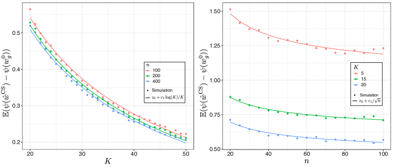
Figure E.1: $\mathbb{E}(\psi(\hat{w}^{\text{CS}})-\psi(w_{g}^{0}))$ as a function of $K$ and $n$. Dots represent results from the Monte Carlo simulation. Lines illustrate the fitted functions $c_{0}+c_{1}\log(K)/K$ (Left) and $c_{0}+c_{1}/\sqrt{n}$ (Right) to the Monte Carlo results. Simulation settings are described in Section 5.

References

- Babapulle et al. (2004) Babapulle, M. N., L. Joseph, P. Bélisle, J. M. Brophy, and M. J. Eisenberg (2004). A hierarchical bayesian meta-analysis of randomised clinical trials of drug-eluting stents. The Lancet 364(9434), 583–591.
- Breiman (1996) Breiman, L. (1996). Stacked regressions. Machine learning 24(1), 49–64.
- Higgins et al. (2009) Higgins, J. P., S. G. Thompson, and D. J. Spiegelhalter (2009). A re-evaluation of random-effects meta-analysis. Journal of the Royal Statistical Society: Series A (Statistics in Society) 172(1), 137–159.
- Juditsky and Nemirovski (2000) Juditsky, A. and A. Nemirovski (2000). Functional aggregation for nonparametric regression. Annals of Statistics, 681–712.
- Juditsky et al. (2008) Juditsky, A., P. Rigollet, A. B. Tsybakov, et al. (2008). Learning by mirror averaging. The Annals of Statistics 36(5), 2183–2206.
- Kannan et al. (2016) Kannan, L., M. Ramos, A. Re, N. El-Hachem, Z. Safikhani, D. M. Gendoo, S. Davis, D. Gomez-Cabrero, R. Castelo, K. D. Hansen, et al. (2016). Public data and open source tools for multi-assay genomic investigation of disease. Briefings in bioinformatics 17(4), 603–615.
- Klein et al. (2014) Klein, R., K. Ratliff, M. Vianello, R. Adams Jr, S. Bahník, M. Bernstein, K. Bocian, M. Brandt, B. Brooks, C. Brumbaugh, et al. (2014). Data from investigating variation in replicability: A ?many labs? replication project. Journal of Open Psychology Data 2(1).
- LeBlanc and Tibshirani (1996) LeBlanc, M. and R. Tibshirani (1996). Combining estimates in regression and classification. Journal of the American Statistical Association 91(436), 1641–1650.
- Loewinger et al. (2019) Loewinger, G. C., K. K. Kishida, P. Patil, and G. Parmigiani (2019). Covariate-profile similarity weighting and bagging studies with the study strap: Multi-study learning for human neurochemical sensing. bioRxiv, 856385.
- Manzoni et al. (2018) Manzoni, C., D. A. Kia, J. Vandrovcova, J. Hardy, N. W. Wood, P. A. Lewis, and R. Ferrari (2018). Genome, transcriptome and proteome: the rise of omics data and their integration in biomedical sciences. Briefings in bioinformatics 19(2), 286–302.
- Moreno-Torres et al. (2012) Moreno-Torres, J. G., T. Raeder, R. Alaiz-RodríGuez, N. V. Chawla, and F. Herrera (2012). A unifying view on dataset shift in classification. Pattern recognition 45(1), 521–530.
- Pasolli et al. (2016) Pasolli, E., D. T. Truong, F. Malik, L. Waldron, and N. Segata (2016). Machine learning meta-analysis of large metagenomic datasets: tools and biological insights. PLoS computational biology 12(7), e1004977.
- Patil et al. (2015) Patil, P., P.-O. Bachant-Winner, B. Haibe-Kains, and J. T. Leek (2015). Test set bias affects reproducibility of gene signatures. Bioinformatics 31(14), 2318–2323.
- Patil and Parmigiani (2018) Patil, P. and G. Parmigiani (2018). Training replicable predictors in multiple studies. Proceedings of the National Academy of Sciences 115(11), 2578–2583.
- Rhodes et al. (2004) Rhodes, D. R., J. Yu, K. Shanker, N. Deshpande, R. Varambally, D. Ghosh, T. Barrette, A. Pandey, and A. M. Chinnaiyan (2004). Large-scale meta-analysis of cancer microarray data identifies common transcriptional profiles of neoplastic transformation and progression. Proceedings of the National Academy of Sciences 101(25), 9309–9314.
- Shumway and Stoffer (2017) Shumway, R. H. and D. S. Stoffer (2017). Time series analysis and its applications: with R examples. Springer.
- Simon et al. (2003) Simon, R., M. D. Radmacher, K. Dobbin, and L. M. McShane (2003). Pitfalls in the use of dna microarray data for diagnostic and prognostic classification. Journal of the National Cancer Institute 95(1), 14–18.
- Sinha et al. (2017) Sinha, R., G. Abu-Ali, E. Vogtmann, A. A. Fodor, B. Ren, A. Amir, E. Schwager, J. Crabtree, S. Ma, C. C. Abnet, et al. (2017). Assessment of variation in microbial community amplicon sequencing by the microbiome quality control (mbqc) project consortium. Nature biotechnology 35(11), 1077.
- Sutton and Higgins (2008) Sutton, A. J. and J. P. Higgins (2008). Recent developments in meta-analysis. Statistics in medicine 27(5), 625–650.
- Tseng et al. (2012) Tseng, G. C., D. Ghosh, and E. Feingold (2012). Comprehensive literature review and statistical considerations for microarray meta-analysis. Nucleic acids research 40(9), 3785–3799.
- van der Laan et al. (2006) van der Laan, M. J., S. Dudoit, and A. W. van der Vaart (2006). The cross-validated adaptive epsilon-net estimator. Statistics & Decisions 24(3), 373–395.
- Warn et al. (2002) Warn, D., S. Thompson, and D. Spiegelhalter (2002). Bayesian random effects meta-analysis of trials with binary outcomes: methods for the absolute risk difference and relative risk scales. Statistics in medicine 21(11), 1601–1623.
- Watson (1983) Watson, G. S. (1983). Statistics on spheres. The University of Arkansas lecture notes in the mathematical sciences ; v. 6. New York: Wiley.
- Wolpert (1992) Wolpert, D. H. (1992). Stacked generalization. Neural networks 5(2), 241–259.
- Zhang (1993) Zhang, P. (1993). Model selection via multifold cross validation. The annals of statistics, 299–313.
- Zhang et al. (2019) Zhang, Y., W. E. Johnson, and G. Parmigiani (2019). Robustifying genomic classifiers to batch effects via ensemble learning. bioRxiv, 703587.