Global dynamics in a predator-prey model with cooperative hunting and Allee effect and bifurcation induced by diffusion and delays

Abstract

We consider the local bifurcation and global dynamics of a predator-prey model with cooperative hunting and Allee effect. For the model with weak cooperation, we prove the existence of limit cycle, heteroclinic cycle at a threshold of conversion rate $p=p^{\#}$. When $p>p^{\#}$, both species go extinct, and when $p<p^{\#}$, there is a separatrix. The species with initial population above the separatrix finally become extinct; otherwise, they coexist or oscillate sustainably. In the case with strong cooperation, we exhibit the complex dynamics of system in three different cases, including limit cycle, loop of heteroclinic orbits among three equilibria, and homoclinic cycle. Moreover, we find diffusion may induce Turing instability and Turing-Hopf bifurcation, leaving the system with spatially inhomogeneous distribution of the species, coexistence of two different spatial-temporal oscillations. Finally, we investigate Hopf and double Hopf bifurcations of the diffusive system induced by two delays.

1 Introduction

A predator-prey model can be described by the following equations Cosner

$$\left\{\begin{array}[]{lll}\dot{u}&=&f(u)u-G(u,v)v,\\ \dot{v}&=&dG(u,v)v-mv,\\ \end{array}\right.$$ (1)

where $u$ and $v$ stand for the densities of prey and predator, respectively. $f(u)$ represents the per capita prey growth rate in the absence of predators, and the function $G(u,v)$ is the functional response charactering predation. $d$ describes the rate of biomass conversion from predation, and $m$ is the death rate of predator. Many kinds of functional response have been proposed Jeschke . Among them Holling type I, II, III C. S. Holling ; N. Kazarinov ; P. Turchin are discussed widely, which are prey-dependent functional response.

Cooperative behavior within a species is very common in nature, of which cooperative hunting is the most widely distributed form in animals. In mammals, the most famous examples include wolves Schmidt , African wild dogs Courchamp , lions Scheel , and chimpanzees C. Boesch , who cooperate for hunting preys. Cooperative behaviors are also widespread in other living organisms, such as aquatic organisms Bshary , spiders Uetz , birds D. P. Hector , and ants Moffett , who find, attack and move their preys together. Due to hunting cooperation, the attack rate of predators increases with predator density, which obviously depends on both prey and predator densities. Recently, a few literatures have paid attention to derive functional response to describe the cooperative hunting Cosner ; Berec ; Alves . Cosner et al. Cosner proposed a functional response to explore the effects of predator aggregation when predators encounter a cluster of prey. Berec Berec generalized the Holling type-II functional response to a family of functional responses by considering attack rate and handling time of predators varies with predator density to interpret the foraging facilitation among predators. Alves and Hilker Alves considered a special case of the more general functional response proposed by Berec Berec . They added a cooperation term to the attack rate for representing the benefits that hunting cooperation brings to the predator population, which makes the functional response $G(u,v)=(b+cv)u$. Here $c>0$ describes the strength of predator cooperation in hunting, where $cy$ is referred to as the cooperation term. They found that cooperative hunting can improve persistence of the predator, and it is a form of foraging facilitation which can induce strong Allee effects. After their work, many predator-prey model with cooperative hunting in the predator have been investigated Jang ; S. Pal ; D. Sen ; S. Yan ; Wu D ; Danxia Song .

The most well-known example of $f(u)$ is the logistic form $f(u)=r\left(1-\frac{u}{K}\right)$, where $r$ is the intrinsic growth rate, $K$ denotes the environmental carrying capacity. Then, in the absence of predator, the prey population is governed by $\dot{u}=ru\left(1-\frac{u}{K}\right)$. We can conclude from the equation that the species may increase in size when the density is low. However, for many species, low population density may induce many problems, such as mate difficulties, inbreeding and predator avoidance of defence. It turns out that the growth rate of the low density population is not always positive, and it may be negative when the density of population is less than the minimum number $a$ for the survival of the population, which is called the Allee threshold. The phenomenon is known as Allee effect, which was first observed by Allee Allee , and has been observed on various organisms, such as vertebrates, invertebrates and plants. Such a population can be described by $\dot{u}=ru\left(1-\frac{u}{K}\right)(u-a)$. Allee effect may cause the extinction of low-density population. Because of increasing fragmentation of habitats, invasions of exotic species, Allee effect has aroused more and more attention (see for example Courchamp F ; Wang2010 ; Conway and the references cited therein).

Jang et al. Jang considered both the cooperation in the predator and Allee effects in the prey, and proposed the following predator-prey model

$$\left\{\begin{array}[]{lll}\dfrac{{\rm d}u}{{\rm d}t}&=&r_{1}u\left[1-\frac{u}{K_{1}}\right]\left[u-a_{1}\right]-\left[b_{1}+c_{1}v\right]uv,\\ \dfrac{{\rm d}v}{{\rm d}t}&=&p_{1}[b_{1}+c_{1}v]uv-m_{1}v,\\ \end{array}\right.$$ (2)

where $r_{1}$ is the per capita intrinsic growth rate of the prey, $K_{1}$ is the enviromental carrying capacity for the prey, $a_{1}$ ($a_{1}<K_{1}$) is the Allee threshold of the prey population, $b_{1}$ is the attack rate per predator and prey, $c_{1}$ measures the degree of cooperation of predator, $p_{1}$ is the prey conversion to predator, and $m_{1}$ is the per capita death rate of predator. They discussed the extinction and and coexistence of the species when the parameters are in different ranges, and found that cooperation hunting might change the number of equilibria and change that stability of the interior equilibria. They also devised a best strategy for culling the predator by maximizing the prey population and minimizing the predators along with the costs associated with the control.

With a nondimensionalized change of variables:

$$\widehat{u}=\frac{1}{K}u,~{}\widehat{v}=bv,$$

and dropping the hats for simplicity of notations, system (2) takes the form

$$\left\{\begin{array}[]{l}\dfrac{{\rm d}u}{{\rm d}t}=K_{1}r_{1}u[1-u](u-\frac{a_{1}}{K_{1}})-(1+\frac{c_{1}}{b_{1}^{2}}v)uv,\\ \dfrac{{\rm d}v}{{\rm d}t}=m_{1}v\left[\frac{b_{1}p_{1}K_{1}}{m_{1}}u\left(1+\frac{c_{1}}{b_{1}^{2}}v\right)-1\right].\end{array}\right.$$

Let

$$r=K_{1}r_{1},~{}~{}a=\frac{a_{1}}{K_{1}},~{}~{}c=\frac{c_{1}}{b_{1}^{2}},~{}~{}\mbox{and}~{}~{}p=\frac{b_{1}p_{1}K_{1}}{m_{1}}.$$

Then we obtain the simplified dimensionless system

$$\left\{\begin{array}[]{l}\dfrac{{\rm d}u}{{\rm d}t}=ru(1-u)(u-a)-(1+cv)uv,\\ \dfrac{{\rm d}v}{{\rm d}t}=mv\left[pu\left(1+cv\right)-1\right].\\ \end{array}\right.$$ (3)

Recall the definition of Allee effect, one always has $0<a<1$. In fact, for fixed $K_{1}$, $r_{1}$, $a_{1}$, $b_{1}$ and $m_{1}$, we have $c$ and $p$ directly proportional to $c_{1}$ and $p_{1}$, respectively. Thus, we refer to $c$ and $p$ as the degree of cooperative hunting of the predator and the conversion rate from the prey to the predator respectively in the context. By the explanation above, we make the following assumption always:

$$(H)~{}~{}~{}~{}~{}~{}r,~{}~{}a,~{}~{}c,~{}~{}m,~{}~{}p~{}\mbox{and}~{}c~{}~{}\mbox{are all positive, and}~{}~{}0<a<1.$$

Motivated by Jang , in this paper, we will consider a complete global analysis of the model (3) by investigating the stable/unstable manifolds of saddles, then the existence of some connecting orbits is obtained. Hence, a partition of the phase space is given, i.e., the attraction basin of each equilibrium is obtained.

This paper is organized as follows. In section 2, we investigate the global dynamics of the ODE predator-prey model (3) with weak cooperation and strong cooperation respectively. Firstly, for the case of weak cooperation, the existence and stability of equilibria are discussed. Taking $p$ as the bifurcation parameter, the existence of Hopf bifurcation and loop of heteroclinic orbits is proved, and the global dynamics are investigated. For the case with strong cooperation, the existence of Hopf bifurcation, loop of heteroclinic orbits, and homoclinic cycle are observed by theoretical analysis or numerical simulation. In section 3, we consider the diffusive system (11), and investigate Turing instability and Turing-Hopf bifurcation induced by diffusion. We illustrate some complex dynamics of system, including the existence of spatial inhomogeneous steady state, coexistence of two spatial inhomogeneous periodic solutions. In section 4, we consider the diffusive system with two delays, and Hopf bifurcation and double Hopf bifurcation induced by two delays are analyzed on the center manifold via normal form approach.

2 Global dynamics of the ODE system

In this section, we consider the ODE system (3) with two different cases. It is found that the strength of cooperation heavily affects the number of interior equilibria. Thus, the theoretical results are given on two cases: when $c<\frac{1}{r(1-a)}$, we say the cooperation among predators is weak; when $c>\frac{1}{r(1-a)}$, the cooperation is strong. We investigate the local and global dynamics in both cases, together with some numerical illustrations, as well as biological interpretations.

2.1 The system with weak cooperative hunting

In this section, we first consider the existence of boundary equilibria and interior equilibria, respectively. Then, taking $p$ as bifurcation parameter, we investigate the Hopf bifurcation near the unique interior equilibrium. Through studying the stable manifold and unstable manifold of saddles, we prove the existence of loop of heteroclinic orbits, and get the global dynamics of system (3).

For model (3), the first quadrant is invariant since $\{(u,v):u=0\}$ and $\{(u,v):v=0\}$ are invariant manifolds for (3). We can get the following result.

      Lemma 1.

The solution of (3) with positive initial value is positive and bounded.

Proof. For any $u(0)>1$, $u^{\prime}=ru(1-u)(u-a)-(1+cv)uv<0$ if $u>1$. On $u=1$, $u^{\prime}<-(1+cv)v<0$. Noticing that there is no equilibrium in the region $\{(u,v):u>1,v\geq 0\}$, any positive solution satisfies $u(t)\leq\max\{u(0),1\}$ for $t\geq 0$. From (3), we obtain that $(mpu+v)^{\prime}=mpru(1-u)(u-a)-mv\leq mpru(1-u)(u-a)+m^{2}pu-m(mpu+v)\leq\zeta-m(mpu+v)$, where $\zeta=\max_{t\geq 0}\{mpru(1-u)(u-a)+m^{2}pu\}$. Then we have $mpu(t)+v(t)\leq(mpu(0)+v(0))e^{-mt}+\frac{\zeta}{m}(1-e^{-mt})$, which means that $v(t)$ is bounded.

2.1.1 Existence of equilibria

System (3) has three boundary equilibria: (i) $E_{0}(0,0)$, which means the extinction of both the species; (ii) $E_{a}(a,0)$, which is induced by Allee effect; (iii) $E_{1}(1,0)$, which means the extinction of the predator and the survival of the prey, achieving its carrying capacity.

Now we discuss the existence of interior equilibria similar as the discussion in Jang . The existence of interior equilibria depends on the position of $u-$nullcline $r(1-u)(u-a)=(1+cv)v$ and $v-$nullcline $pu(1+cv)=1$. In fact, $r(1-u)(u-a)=(1+cv)v$ is an ellipse, sitting in the first and forth quadrant, and intersecting the horizontal axis at $a$ and $1$. $pu(1+cv)=1$ is hyperbolic, with its right branch sitting in the first and forth quadrant and intersecting the horizontal axis at $\frac{1}{p}$, and is decreasing and concave in $(0,\frac{1}{p})$. Denote the $u-$nullcline curve $r(1-u)(u-a)=(1+cv)v$ in the first quadrant as $v=f(u)$, the $v-$nullcline curve $pu(1+cv)=1$ in the first quadrant as $v=g(u)$. Obviously, an intersection of $v=f(u)$ and $v=g(u)$ is an interior equilibrium, thus any interior equilibrium has components $u>0$ and $v>0$ satisfying

$$\begin{array}[]{rl}r(1-u)(u-a)&=(1+cv)v,\\ pu(1+cv)&=1,\end{array}$$ (4)

i.e.,

$$\begin{array}[]{rl}r(1-u)(u-a)&=\frac{1-pu}{cp^{2}u^{2}},\\ v&=\frac{1-pu}{cpu}.\end{array}$$ (5)

The existence of interior equilibria may have the following different cases.

Proposition 1.

Suppose that $c<\frac{1}{r(1-a)}$.
       (i) When $p\geq\frac{1}{a}$, system (3) has no interior equilibria.
       (ii) When $1<p<\frac{1}{a}$, system (3) has a unique positive constant equilibrium $E^{*}(u^{*},v^{*})$ with $a<u^{*}<\frac{1}{p}$.
       (iii) When $p\leq 1$, system (3) has no interior equilibria.

Proof. In fact, when $a<\frac{1}{p}<1$, two nullclines have two intersections, $E^{*}$ in the first quadrant (see Fig. 1 b)) and $E_{R}^{*}$ in the forth quadrant. Thus there is a unique interior equilibrium $E^{*}(u^{*},v^{*})$ with $u^{*}$ and $v^{*}$ satisfying (4). When $\frac{1}{p}$ decreases to $a$, $E^{*}$ collides with $E_{a}$, and $E_{R}^{*}$ is still in the forth quadrant. When $\frac{1}{p}<a$, $E^{*}$ moves into the forth quadrant, leaving no interior equilibria (see Fig. 1 a)).

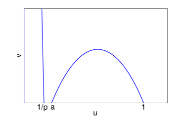
a) b)

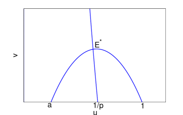
Figure 1: a) When $p>\frac{1}{a}$, there is no interior equilibrium. b) When $1<p<\frac{1}{a}$, there is a unique interior equilibrium.

When $\frac{1}{p}$ increases to $1$, the $v-$nullcline $v=g(u)$ and $u-$nullcline $v=f(u)$ intersect at $E_{1}(1,0)$. The slope of tangents of $v-$nullcline and $u-$nullcline at $E_{1}(1,0)$ are $-\frac{1}{c}$ and $-r(1-a)$ respectively. If $-\frac{1}{c}<-r(1-a)$, $E^{*}$ collides with $E_{1}$ when $p=1$ (see Fig. 2 a)), $E_{R}^{*}$ is in the forth quadrant, and there is no interior equilibria. Moreover, when $p<1$, there is no interior equilibria (see Fig. 2 b)). $~{}~{}~{}~{}~{}~{}~{}~{}~{}~{}~{}~{}~{}~{}~{}~{}~{}~{}~{}~{}~{}~{}~{}~{}~{}~{}~{}~{}~{}~{}~{}~{}~{}~{}~{}~{}~{}~{}~{}~{}~{}~{}~{}~{}~{}~{}~{}~{}~{}~{}~{}~{}~{}~{}~{}~{}~{}~{}~{}~{}~{}~{}\Box$

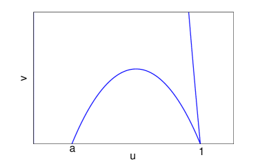
a) b)

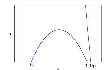
Figure 2: If $c<\dfrac{1}{r(1-a)}$, there is a) no interior equilibrium when $p=1$; b) no interior equilibrium when $p<1$.

There is always a unique positive equilibrium $E^{*}(u^{*},v^{*})$ when $1<p<\frac{1}{a}$. Now we wonder the impact of $c$ on the value of the component of the unique equilibrium $E^{*}(u^{*},v^{*})$ when $1<p<\frac{1}{a}$, and we have the following conclusion.

Proposition 2.

When $1<p<\frac{1}{a}$, for the unique positive equilibrium $E^{*}(u^{*},v^{*})$ ($a<u^{*}<\frac{1}{p}$), $u^{*}$ is monotonically decreasing with respect to $c$; $v^{*}$ is monotonically decreasing with respect to $c$ when $a<u^{*}<\frac{a+1}{2}$, and it is monotonically increasing when $\frac{a+1}{2}<u^{*}<1$.

Proof. Consider both sides of the first equation of (5) as functions of $u$, denoted by $y=\frac{1-pu}{cp^{2}u^{2}}$ and $y=r(1-u)(u-a)$. Obviously, The $u-$component of interaction of $y=r(1-u)(u-a)$ and $y=\frac{1-pu}{cp^{2}u^{2}}$ moves left when the value of $c$ increases. It means that $u^{*}$ is monotonically decreasing with respect to $c$.

Now we focus on the effect of $c$ on the $v^{*}$ component of the interior equilibrium. Since $r(1-u^{*})(u^{*}-a)=\frac{1-pu^{*}}{cp^{2}u^{*2}}$, and $v^{*}=\frac{1-pu^{*}}{cpu^{*}}$, then $v^{*}=rpu^{*}(1-u^{*})(u^{*}-a)$. With the increasing of $c$, $u^{*}$ decreases. If $\frac{a+1}{2}>u^{*}>a$, $v^{*}$ is increasing with respect to $u^{*}$, thus it is decreasing with $c$. If $\frac{a+1}{2}<u^{*}<1$, $v^{*}$ is decreasing with $u^{*}$, and thus it is increasing with $c$. $~{}~{}~{}~{}~{}~{}~{}~{}~{}~{}~{}~{}~{}~{}~{}~{}~{}~{}~{}~{}~{}~{}~{}~{}~{}~{}~{}~{}~{}~{}~{}~{}~{}~{}~{}~{}~{}~{}~{}~{}~{}~{}~{}~{}~{}~{}~{}~{}~{}~{}~{}~{}~{}~{}~{}~{}~{}~{}~{}~{}~{}~{}~{}~{}~{}~{}~{}~{}~{}~{}~{}~{}~{}~{}\Box$

      Remark 1.

In the absence of cooperative hunting within the predator, i.e., $c=0$, system (3) always has a unique interior equilibrium $E_{0}^{*}=(\frac{1}{p},r(1-\frac{1}{p})(\frac{1}{p}-a))$, and $E_{0}^{*}$ exists if and only if $1<p<\frac{1}{a}$. The cooperative hunting $c$ may change the density of prey and predator. It is not surprising that the increasing of cooperative hunting will decrease the density of the prey. When $\frac{a+1}{2}<u^{*}<1$, cooperative hunting is beneficial to the density of predator. However, when $a<u^{*}<\frac{a+1}{2}$, the cooperative hunting will decrease the stationary density of the predator.

2.1.2 Stability of all equilibria and Hopf bifurcation at $E^{*}$

The Jacobian matrices of the function on the right-hand of system (3) around $E_{0}$, $E_{a}$, and $E_{1}$ are respectively,

$$J_{E_{0}}=\left(\begin{array}[]{cc}-ra&0\\ 0&-m\end{array}\right),$$

$$J_{E_{a}}=\left(\begin{array}[]{cc}ra(1-a)&-a\\ 0&m(pa-1)\end{array}\right),$$

$$J_{E_{1}}=\left(\begin{array}[]{cc}-r(1-a)&-1\\ 0&m(p-1)\end{array}\right),$$

from which we can easily get the local stability of the boundary equilibria.

      Lemma 2.

For system (3),
      (i) $E_{0}(0,0)$ is a stable node;
      (ii) $E_{a}(a,0)$ is an unstable node if $p>\frac{1}{a}$, and it is a saddle if $p<\frac{1}{a}$;
      (iii) $E_{1}(1,0)$ is a stable node if $p<1$, and it is a saddle if $p>1$.

For the interior equilibrium $E^{*}(u^{*},v^{*})$, the corresponding Jacobian matrix is

$$J_{E^{*}}=\left(\begin{array}[]{cc}ru^{*}(1+a-2u^{*})&-2cu^{*}v^{*}-u^{*}\\ mpv^{*}(1+cv^{*})&mpcu^{*}v^{*}\end{array}\right),$$ (6)

and thus

$$\begin{array}[]{l}{\rm tr}J_{E^{*}}=-ru^{*}(2u^{*}-a-1)+mpcu^{*}v^{*}=-ru^{*}(2u^{*}-a-1)+m(1-pu^{*}),\\ {\rm det}J_{E^{*}}=mpu^{*}v^{*}\left[rcu^{*}(1+a-2u^{*})+(1+cv^{*})(1+2cv^{*})\right].\end{array}$$

In fact, $u-$nullcline $v=f(u)$ and $v-$nullcline $v=g(u)$ intersect at $E^{*}$, where the slope of $v=f(u)$ is larger than that of $v=g(u)$, i.e., $\dfrac{1+cv^{*}}{-cu^{*}}<\dfrac{r(1+a-2u^{*})}{1+2cv^{*}}$. Thus, ${\rm det}J_{E^{*}}>0$. Thus $E^{*}$ may be node or focus, and its stability depends on the trace

$${\rm tr}J_{E^{*}}=-ru^{*}(2u^{*}-a-1)+m(1-pu^{*}).$$ (7)

Thus, we have the following conclusions on the stability of $E^{*}$.

      Theorem 1.

If $c<\frac{1}{r(1-a)}$, then there exists a unique $p_{H}\in(1,\frac{2}{a+1})$ such that the unique interior equilibrium $E^{*}$ is locally asymptotically stable when $1<p<p_{H}$, and unstable when $p_{H}<p<\frac{1}{a}$. Moreover, system (3) undergoes a Hopf bifurcation at $E^{*}$ when $p=p_{H}$.

Proof. Solving for ${\rm tr}J_{E^{*}}=0$, when $\frac{a+1}{2}<\frac{1}{p}<1$, we obtain a unique $u_{H}^{*}\in(\frac{a+1}{2},1)$, such that ${\rm tr}J_{E^{*}}>0$ on $(0,u_{H}^{*})$, and ${\rm tr}J_{E^{*}}<0$ on $(u_{H}^{*},1)$ (see Fig. 3). Moreover, it is easy to verify that $\frac{\partial u^{*}}{\partial p}<0$, thus, corresponding to $u_{H}^{*}$, we obtain a unique $p_{H}$ ($1<p_{H}<\frac{2}{a+1}$), such that ${\rm tr}J_{E^{*}}>0$ when $p\in(p_{H},\frac{1}{a})$, and ${\rm tr}J_{E^{*}}<0$ when $p\in(1,p_{H})$.

Now we verify the transversality condition. Let $\mu=\alpha(p)\pm i\omega(p)$ be the roots of $\mu^{2}-{\rm tr}J_{E^{*}}\mu+{\rm det}J_{E^{*}}=0$ when $p$ is near $p_{H}$. We have $\alpha^{\prime}(p)=\frac{1}{2}\frac{{\rm d}{\rm tr}J_{E^{*}}}{{\rm d}p}=\frac{1}{2}[-ru^{*^{\prime}}(p)(2u^{*}-a-1)-2ru^{*}u^{*^{\prime}}(p)$$-mu^{*}-mpu^{*^{\prime}}(p)]$ , where $u^{*}(p)$ is a function of $p$ determined by (5). Taking the derivative of both sides of (5) with respect to $p$, we have

$$-ru^{*^{\prime}}(p)(2u^{*}-a-1)=\dfrac{(-u-pu^{*^{\prime}}(p))[cp^{2}u^{*2}+2cpu^{*}(1-pu^{*})]}{c^{2}p^{4}u^{*4}},$$

thus

$$-u-pu^{*^{\prime}}(p)\mid_{p=p_{H}}=\dfrac{-ru^{*^{\prime}}(p)(2u^{*}-a-1)c^{2}p^{4}u^{*4}}{cp^{2}u^{*2}+2cpu^{*}(1-pu^{*})}\mid_{p=p_{H}}>0,$$

since $\frac{a+1}{2}<u_{H}^{*}<\frac{1}{p}$ and $u^{*^{\prime}}(p)<0$. Thus, $\alpha^{\prime}(p)\mid_{p=p_{H}}>0$. $~{}~{}~{}~{}~{}~{}~{}~{}~{}~{}~{}~{}~{}~{}~{}~{}~{}~{}~{}~{}~{}~{}~{}~{}~{}~{}~{}~{}~{}~{}~{}~{}~{}~{}~{}~{}~{}~{}~{}~{}~{}~{}~{}~{}~{}~{}\Box$

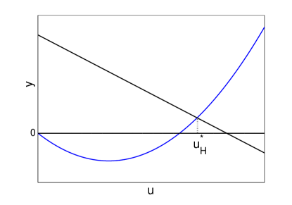
Figure 3: The blue curve represents $y=ru^{*}(2u^{*}-a-1)$, and the black line represents $y=m(1-pu^{*})$. When $u=u_{H}^{*}$, ${\rm tr}J_{E^{*}}=0$.

      Remark 2.

When there is no cooperative hunting in predator, i.e., $c=0$, the $v-$nullcline is $u=\frac{1}{p}$, which is vertical. ${\rm tr}J_{E^{*}}\arrowvert_{c=0}=-\frac{r}{p}(\frac{2}{p}-a-1),{\rm det}J_{E^{*}}\arrowvert_{c=0}=mv^{*}.$ The system undergoes a Hopf bifurcation near $E^{*}$ when $\frac{1}{p}=\frac{a+1}{2}$, which is the top of the $u-$nullcline $v=r(1-u)(u-a)$. In fact, it has been discussed widely that the stability of positive equilibrium can be stated graphically by the $u-$nullcline when the $v-$nullcline is vertical: $(u^{*},v^{*})$ is unstable if the $v-$nullclines intersect to the left of a local maximum of the $u-$nullcline, and stable if they intersect to the right Rosenzweig ; Rosenzweig1969 ; Hsu SB ; Wang2010 , and thus, Hopf bifurcation occurs at the “top of the hump” of $u-$nullcline. However, for system (3) in this paper, the $v-$nullcline is not vertical, and we can verify that the intersection of the $u$-nullcline and the $v$-nullcline corresponding to the Hopf bifurcation point $p=p_{H}$ is on the right of the “top of the hump” of $u$-nullcline. In fact, the “top of the hump” of $u-$nullcline $v=f(u)$ achieves at $u=\frac{a+1}{2}$, at which the corresponding value of $p$ is denoted by $p_{{\rm top}}$. When $p=p_{\rm top}$, $E^{*}$ can be also proved to be unstable. Comparing the results in systems with and without cooperation, we can conclude that cooperative hunting is more likely to bring instability into $E^{*}$.

In order to determine the direction of Hopf bifurcation and the stability of the Hopf bifurcating periodic solution, we need to calculate the normal form near the Hopf bifurcation point. Through direct calculation following the steps in Wiggins S , we can get the following truncated normal form

$$\begin{array}[]{l}\dot{r}=\alpha^{\prime}(p_{H})pr+a(p_{H})r^{3}+O(r|p-p_{H}|^{2},r^{3}|p-p_{H}|,r^{5}),\\ \dot{\theta}=\omega(p_{H})+\omega^{\prime}(p_{H})(p-p_{H})+c(p_{H})r^{2}+O(|p-p_{H}|^{2},r^{2}|p-p_{H}|,r^{4}).\end{array}$$

Recalling that $\alpha^{\prime}(p_{H})>0$, the direction of Hopf bifurcation and stability of Hopf bifurcating periodic solution are determined by the first Lyapunov coefficient $a(p_{H})$, and we have the following conclusion.

      Theorem 2.

System (3) undergoes a Hopf bifurcation at $E^{*}$ when $p=p_{H}$.
       (i) If $a(p_{H})<0$, the bifurcating periodic solution is orbitally asymptotically stable, and it is bifurcating from $E^{*}$ as $p$ increases and passes $p_{H}$.
       (ii) If $a(p_{H})>0$, the bifurcating periodic solution is unstable, and it is bifurcating from $E^{*}$ as $p$ decreases and passes $p_{H}$.

2.1.3 The global dynamics of system (3) with weak cooperative hunting

From the previous discussion, we have known the stability of all equilibria when $c<\frac{1}{r(1-a)}$, which is listed in Table 1. Motivated by the work of Wang2010 ; Conway , we investigate the global dynamics of system (3) when $c<\frac{1}{r(1-a)}$.

Table 1: Stability of equilibria of (3) when $c<\frac{1}{r(1-a)}$.

Equilibrium	$p>\frac{1}{a}$	$p_{H}<p<\frac{1}{a}$	$1<p<p_{H}$	$p<1$
$E_{0}(0,0)$	stable node	stable node	stable node	stable node
$E_{a}(a,0)$	unstable node	saddle	saddle	saddle
$E_{1}(1,0)$	saddle	saddle	saddle	stable node
$E^{*}(u^{*},v^{*})$	does not exist	unstable node or focus	stable node or focus	does not exist

When $p<\frac{1}{a}$, $E_{a}$ is a saddle. The eigenvector corresponding to $\lambda_{1}=ra(1-a)>0$ is $(1,0)$, which means that the unstable manifold of $E_{a}$ is on the $u$-axis. For $\lambda_{2}=m(pa-1)<0$, the corresponding eigenvector is $(1,r(1-a)-\frac{m(pa-1)}{a})^{T}$. Thus the tangent vector of the stable manifold of $E_{a}(a,0)$ (denoted by $\Gamma_{p}^{s}$) at $E_{a}(a,0)$ is $k_{1}=r(1-a)-\frac{m(pa-1)}{a}$. Comparing with the tangent vector $k_{2}=r(1-a)$ of $v=f(u)$ at $E_{a}(a,0)$, we have $k_{1}>k_{2}$, thus $\Gamma_{p}^{s}$ is above the nullcline $v=f(u)$ near $E_{a}$. Moreover, from the vector field in (3) on $v=f(u)$, $\Gamma_{p}^{s}$ is always above $v=f(u)$ before $\Gamma_{p}^{s}$ meets the $v-$nullcline.

Similarly, when $p>1$, $E_{1}$ is a saddle. Its stable manifold is on the $u-$axis, and its unstable manifold, $\Gamma_{p}^{u}$, is above the nullcline $v=f(u)$ before it meets the $v-$nullcline.

When $1<p<\frac{1}{a}$, $E_{0}$ and $E_{a}$ are all saddle points. To figure out the global dynamics of system (3), we should first study the stable manifold $\Gamma_{p}^{s}$ of $E_{a}$ and unstable manifold $\Gamma_{p}^{u}$ of $E_{1}$.

Proposition 3.

Suppose that $c<\frac{1}{r(1-a)}$, and $1<p<\frac{1}{a}$.
       (i) The orbit $\Gamma_{p}^{s}$ meets the $v-$nullcline $v=g(u)$ at a point $(u_{p}^{s},S(p))$, where $S(p)\geq v^{*}:=f(u^{*})$, and $S(p)$ is a monotone decreasing function for $p\in(1,\frac{1}{a})$.
       (ii) The orbit $\Gamma_{p}^{u}$ meets the $v-$nullcline $v=g(u)$ at a point $(u_{p}^{u},U(p))$, where $U(p)\geq v^{*}:=f(u^{*})$, and $U(p)$ is a monotone increasing function for $p\in(1,\frac{1}{a})$.

Proof. Inspired by Wang2010 , we prove (i), and the proof for (ii) is similar. We have proved that $\Gamma_{p}^{s}$ approaches $E_{a}$ from the region $\{(u,v):v>f(u)\}$. Moreover, $\Gamma_{p}^{s}$ is always above $v=f(u)$ before $\Gamma_{p}^{s}$ meets the $v-$nullcline. In order to show that $\Gamma_{p}^{s}$ meets the $v-$nullcline, we still need to prove that it remains bounded for $u>a$. In fact, for $u>a$, $\Gamma_{p}^{s}$ is the graph of a function $v(u)$, satisfying

$$\dfrac{{\rm d}v(u)}{{\textrm{d}}u}=\dfrac{mv[1-pu(1+cv)]}{u[(1+cv)v-r(1-u)(u-a)]}.$$

If there is a $u_{b}<u^{*}$ such that $v(u)\rightarrow\infty$ as $u\rightarrow u_{b}^{-}$, then $(1+cv)v-r(1-u)(u-a)$ is bounded below for $a+\varepsilon\leq u\leq u_{b}$ and any $\varepsilon>0$. Thus for $a+\varepsilon\leq u\leq u_{b}$,

$$\dfrac{{\rm d}v}{{\rm d}u}\leq Av$$

for some positive constant $A$. It means that $v(u)$ is bounded as $u\rightarrow u_{b}^{-}$, which is a contradiction. Thus it cannot blow up before it extends to the $v-$nullcline $v=g(u)$. Therefore, $S(p)$ exists for all $p\in(1,\frac{1}{a})$ and $S(p)\geq v^{*}$.

Notice that $S(p)=v^{*}$ only when $\Gamma_{p}^{s}\rightarrow E^{*}$ as $t\rightarrow-\infty$, which means $E^{*}$ must be an unstable node. When $1<p<p_{H}$, $E^{*}$ is locally stable, thus $S(p)>v^{*}$ if $p<p_{H}$. When $p_{H}<p<\frac{1}{a}$ and near $p_{H}$, $E^{*}$ is an unstable spiral. Thus, the set $K=\{p\in(1,\frac{1}{a}):S(p)>v^{*}\}$ is a nonempty open set containing $(1,p_{H}+\varepsilon)$.

Now we show that $S(p)$ is monotonically decreasing on any component of $K$. Let $p_{1}<p_{2}$ be two points in some interval in $K$. Denote the $v-$nullcline for $p_{1}$ and $p_{2}$ as $v=g_{1}(u)$ and $v=g_{2}(u)$. From the expression of $v=g(u)$, we know that the curve of $v=g_{1}(u)$ is on the right of $v=g_{2}(u)$. The stable manifold of $E_{a}(a,0)$ for $p_{1}$ and $p_{2}$ are graphs of function $v_{1}(u)$ and $v_{2}(u)$ defined for $u>a$ respectively. The corresponding eigenvectors at $E_{a}$ are $x_{1}=(1,r(1-a)-\frac{m(p_{1}a-1)}{a})^{T}$, $x_{2}=(1,r(1-a)-\frac{m(p_{2}a-1)}{a})^{T}$, respectively. Hence, $v_{1}(u)>v_{2}(u)$ for $u$ sufficiently near $a$. Suppose that $v_{1}(u)=v_{2}(u)$ for some $u$ with $a<u\leq\frac{1}{p_{2}}$. Let $\overline{u}$ be the smallest such value. Then we must have $v^{\prime}_{2}(\overline{u})\geq v^{\prime}_{1}(\overline{u})\geq 0$. But $\dfrac{mv_{1}(\overline{u})[1-p_{1}\overline{u}(1+cv_{1}(\overline{u}))]}{\overline{u}[(1+cv_{1}(\overline{u}))v_{1}(\overline{u})-r(1-\overline{u})(\overline{u}-a)]}\leq\dfrac{mv_{2}(\overline{u})[1-p_{2}\overline{u}(1+cv_{2}(\overline{u}))]}{\overline{u}[(1+cv_{2}(\overline{u}))v_{2}(\overline{u})-r(1-\overline{u})(\overline{u}-a)]}$ implies that $p_{1}\geq p_{2}$, which is a contradiction. Thus, the intersection of $v_{2}(u)$ and $g_{2}(u)$, $S(p_{2})$, is below the intersection of $v_{1}(u)$ and $g_{2}(u)$. For $v_{1}(u)$ between $g_{2}(u)$ and $g_{1}(u)$, from the vector field on the left of $g_{1}(u)$, the intersection of $v_{1}(u)$ and $g_{1}(u)$, $S(p_{1})$, is higher than that of $v_{1}(u)$ and $g_{2}(u)$. Thus, $S(p_{2})<S(p_{1})$. Notice that the argument above shows that if $p_{2}\in K$ and $S(p_{2})>v^{*}$, then any $p\in(1,p_{2})$ also belongs to $K$ and $S(p)>S(p_{2})$.

We can claim now $K=(1,p_{a})$ for some $p_{a}\in(p_{H},\frac{1}{a})$. For $p\in(1,p_{a})$, $S(p)>v^{*}$, and for $p\in[p_{a},\frac{1}{a})$, $S(p)=v^{*}$. It remains to prove $S(p)$ is decreasing when $p\in[p_{a},\frac{1}{a})$. From the vector field in (3), $\Gamma_{p}^{s}$ moves towards the upper right, backward, before it meets the $v-$nullcline. Then, for $p=p_{{\rm top}}$, we have $S(p)>v^{*}$, and thus $p_{\rm top}<p_{a}$. It is obvious that $v^{*}$ is decreasing with respect to $p$ for $p\in(p_{{\rm top}},\frac{1}{a})$, and thus so does for $p\in[p_{a},\frac{1}{a})$. Therefore, $S(p)$ is decreasing for both $(1,p_{a})$ and $[p_{a},\frac{1}{a})$. $~{}~{}~{}~{}~{}~{}~{}~{}~{}~{}~{}~{}~{}~{}~{}~{}~{}~{}~{}~{}~{}~{}~{}~{}~{}~{}~{}~{}~{}~{}~{}~{}~{}~{}~{}~{}~{}~{}~{}~{}~{}~{}~{}~{}~{}~{}~{}~{}~{}~{}~{}~{}~{}\Box$

From the monotonicity of $U(p)$ and $S(p)$, we have the following result.

Proposition 4.

If $c<\frac{1}{r(1-a)}$, then there exists a unique $p^{\#}\in(1,\frac{1}{a})$, such that $\Gamma_{p^{\#}}^{s}=\Gamma_{p^{\#}}^{u}$, forming a heteroclinic orbit from $E_{1}$ to $E_{a}$.

Proof. Notice that

$$\lim_{p\rightarrow\frac{1}{a}^{-}}(S(p)-U(p))<0,{\rm and}\lim_{p\rightarrow 1^{+}}(S(p)-U(p))>0.$$

From the monotonicity of $S$ and $U$, there exists a unique $p^{\#}$ such that $S(p^{\#})=U(p^{\#})$. $\Box$

In fact, there is another heteroclinic orbit from $E_{a}$ to $E_{1}$, which is formed by the unstable manifold of $E_{a}$ and the stable manifold of $E_{1}$ on the $u-$axis. Thus, there is a loop of heteroclinic orbits from $E_{1}$ to $E_{a}$, and then back to $E_{1}$.

Obviously, $p^{\#}$ is a threshold value of the property of $\Gamma_{p}^{s}$ and $\Gamma_{p}^{u}$. When $p<p^{\#}$, $\Gamma_{p}^{s}$ is above $\Gamma_{p}^{u}$, and when $p>p^{\#}$, $\Gamma_{p}^{s}$ is below $\Gamma_{p}^{u}$. Let $\Omega_{1}$ denotes the bounded open subset of the positive quadrant, bounded by $\Gamma_{p}^{s}$, $v-$nullcline between $\Gamma_{p}^{s}$ and $\Gamma_{p}^{u}$, $\Gamma_{p}^{u}$, and the segment from $E_{1}$ to $E_{a}$ on the $u-$axis (see Fig.4).

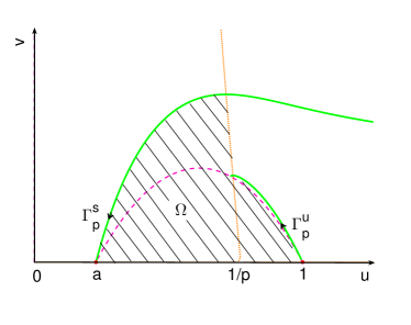
a) b)

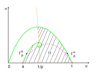
Figure 4: The dashed curve is the $u-$nullcline, and the dotted curve is the $v-$nullcline. Different positions of the stable manifold $\Gamma_{p}^{s}$ of $E_{a}$ and the unstable manifold $\Gamma_{p}^{u}$ of $E_{1}$ for a)$1<p<p^{\#}$ and b) $p^{\#}<p<\frac{1}{a}$.

Proposition 5.

Suppose that $c<\frac{1}{r(1-a)}$.
       (i) If $1<p<p^{\#}$, then $S(p)>U(p)$. Moreover, all orbits in the positive quadrant above $\Gamma_{p}^{s}$ converge to $E_{0}$, and all orbits below $\Gamma_{p}^{s}$ have their $\omega-$limit sets in $\Omega_{1}$, which is a positive invariant set.
       (ii) If $p^{\#}<p<\frac{1}{a}$, then $S(p)<U(p)$, and $\Gamma_{p}^{u}$ tends to $E_{0}$. Moreover, all orbits in the positive quadrant above $\Gamma_{p}^{u}$ converge to $E_{0}$, and all orbits below $\Gamma_{p}^{u}$ have their $\alpha-$limit sets in $\Omega_{1}$, which is a negative invariant set.

Proof. We prove the case for $1<p<p^{\#}$, and the other case can be proved similarly. Propositions 3 and 4 directly lead to $S(p)>U(p)$. From Proposition 3, $\Gamma_{p}^{s}$ enters $E_{a}$ from the region above the $u-$nullcline $v=f(u)$, and meets the $v-$nullcline at $(u_{p}^{s},S(p))$. On the right of $(u_{p}^{s},S(p))$, $\Gamma_{p}^{s}$ is still above $v=f(u)$, since $\Gamma_{p}^{u}$ is above the $u-$nullcline and $S(p)>U(p)$. Moreover, $\Gamma_{p}^{s}$ can not tend to $E_{1}$. In fact, from the direction of the vector field in system (3), $\Gamma_{p}^{s}$ goes to the lower right as $t\rightarrow-\infty$. Thus, $\Gamma_{p}^{s}$ divides the first quadrant into two regions. Noticing that the first quadrant is invariant, we can get the results from Poncaré-Bendixson theorem. $\Box$

Moreover, Poincaré-Bendixson theorem yields the following conclusion.

Proposition 6.

Suppose that $c<\frac{1}{r(1-a)}$.
       (i) If $1<p<p^{\#}$, then either $E^{*}$ is stable or $\Omega_{1}$ contains a periodic orbits which is stable from the outside (both may be true).
       (ii) If $p^{\#}<p<\frac{1}{a}$, then either $E^{*}$ is unstable or $\Omega_{1}$ contains a periodic orbits which is unstable from the outside (both may be true).

From proposition 6, in order to figure out the dynamics in $\Omega_{1}$ in detail, we have to consider the existence and nonexistence of periodic orbits. In section 2.1.2, we have discussed the existence of periodic orbits bifurcating from Hopf bifurcation. Now, we consider the nonexistence of periodic orbits.

Proposition 7.

Suppose that $c<\frac{1}{r(1-a)}$.
      (i) There is an $\varepsilon_{1}>0$ such that if $\frac{1}{a}-\varepsilon_{1}<p<\frac{1}{a}$, there is no periodic orbits, and $\Gamma_{p}^{s}$ connects $E^{*}$ to $E_{a}$, which is a heteroclinic orbit.
      (ii) There is an $\varepsilon_{2}>0$ such that if $1<p<1+\varepsilon_{2}$, there is no periodic orbits, and $\Gamma_{p}^{u}$ connects $E_{1}$ to $E^{*}$.

Proof. We prove the case for $p<\frac{1}{a}$ and near $\frac{1}{a}$, and the latter case can be proved similarly. If $S(p)=v^{*}$, $\Gamma_{p}^{s}$ connects $E^{*}$ to $E_{a}$, and there is no periodic orbits. When $S(p)>v^{*}$, denote the intersection of $\Gamma_{p}^{s}$ and $v-$nullcline as $P(u_{p}^{s},S(p))$. It is easy to confirm that there is a $p_{1}$ such that $S(p)=f(u_{p_{1}})$, where $f(u_{p_{1}})$ is the component of the intersection of $u-$nullcline and $v-$nullcline corresponding to $p_{1}$ ( denoted by $P_{1}(u_{p_{1}},f(u_{p_{1}})$). Consider the region with vertices $E_{a}$, $P$, $P_{1}$, $Q_{1}(\frac{1}{p_{1}},0)$, which is a negative invariant region. $P_{1}$ is well defined when $p$ is close to $\frac{1}{a}$ since $S(p)<f(p_{top})$. Since $E^{*}$ is the unique equilibrium in this region, thus if there are periodic orbits, they must encircle $E^{*}$ and lie wholly in this region. However, the divergence of the vector field of (3) is positive for $p\rightarrow\frac{1}{a}^{-}$, since it is $ra(1-a)+m(pa-1)$ at $E_{a}$, which is positive. From Bendixson’s criterion, there is no periodic orbits in the region. Therefore, according to Poincaré Bendixson theorem, $E^{*}$ is the $\alpha-$limit set of $\Gamma_{p}^{s}$. $~{}~{}~{}~{}~{}~{}~{}~{}~{}~{}~{}~{}~{}~{}~{}~{}~{}~{}~{}~{}~{}~{}~{}~{}~{}~{}~{}~{}~{}~{}~{}~{}~{}~{}~{}~{}~{}~{}~{}~{}~{}~{}~{}~{}~{}~{}~{}~{}~{}~{}~{}~{}~{}~{}~{}~{}~{}~{}~{}~{}~{}~{}~{}~{}~{}~{}~{}~{}~{}~{}~{}~{}~{}~{}~{}~{}~{}~{}~{}\Box$

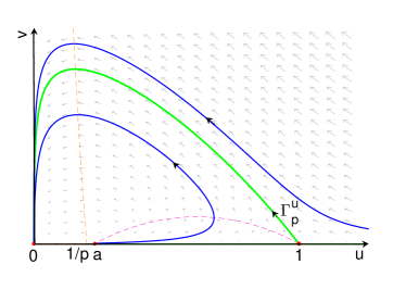
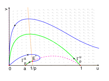
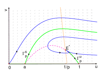
a) b) c) d)

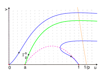
Figure 5: Phase portrait of system (3) for $c<\dfrac{1}{r(1-a)}$ when a) $p>\dfrac{1}{a}$; b) $p<\dfrac{1}{a}$ and close to $\dfrac{1}{a}$; c) $p>1$ and close to $1$; d) and $p<1$.

      Theorem 3.

Suppose that $c<\frac{1}{r(1-a)}$.
       (i) If $p\geq\frac{1}{a}$, $E_{0}(0,0)$ is globally asymptotically stable (see Fig. 5 a) ).
     (ii) There is an $\varepsilon_{1}>0$ such that if $\frac{1}{a}-\varepsilon_{1}<p<\frac{1}{a}$, $\Gamma_{p}^{s}$ connects $E^{*}$ to $E_{a}$, and the extinction equilibrium $E_{0}(0,0)$ is globally asymptotically stable (see Fig. 5 b) ).
     (iii) There is an $\varepsilon_{2}>0$ such that if $1<p<1+\varepsilon_{2}$, then $\Gamma_{p}^{u}$ connects $E_{1}$ to $E^{*}$. The orbits through any point above $\Gamma_{p}^{s}$ converge to $E_{0}$, and the orbits through any point below $\Gamma_{p}^{s}$ converge to $E^{*}$ (see Fig. 5 c) ).
     (iv) If $p<1$, the orbits through any point above $\Gamma_{p}^{s}$ converge to $E_{0}$, and the orbits through any point below $\Gamma_{p}^{s}$ converge to $E_{1}$ (see Fig. 5 d) ).

Proof. (i) If $p\geq\frac{1}{a}$, there is no interior equilibrium, then there is no periodic orbit in the first quadrant. Thus, every orbit converges to a boundary equilibrium. We have known that $E_{0}$ is a stable node, $E_{1}$ is a saddle, and $E_{a}$ is a unstable node if $p>\frac{1}{a}$ and a nonhyperbolic repellor if $p=\frac{1}{a}$. Noting that the first quadrant is positive invariant, then $E_{0}$ is globally asymptotically stable.

(ii) and (iii) follows from proposition 5 and 7 and the fact that $E^{*}$ is a sink when $p>1$ and close to $1$ and a source when $p<\frac{1}{a}$ and close to $\frac{1}{a}$.

(iv) If $p$ decreases to $p=1$, $E^{*}$ collides with $E_{1}$. A transcritical bifurcation involving $E^{*}$ and $E_{1}$ occurs. $E_{1}$ changes its stability from a saddle point to a stable node. If $p<1$, there is no interior equilibrium, and there is no periodic orbit in the first quadrant. $E_{0}$ and $E_{1}$ are both stable node. $E_{a}$ is a saddle, and its stable manifold $\Gamma_{p}^{s}$ divides the first quadrant into two regions. The region above $\Gamma_{p}^{s}$ is the attractive basin of $E_{0}$, and the region below $\Gamma_{p}^{s}$ is the attractive basin of $E_{1}$. $~{}~{}~{}~{}~{}~{}~{}~{}~{}~{}~{}~{}~{}~{}~{}~{}~{}~{}~{}~{}~{}~{}~{}~{}~{}~{}~{}~{}~{}~{}~{}~{}~{}~{}~{}~{}~{}~{}~{}~{}~{}~{}~{}~{}~{}~{}~{}~{}~{}~{}~{}~{}~{}~{}~{}~{}~{}~{}~{}~{}~{}~{}~{}~{}~{}~{}~{}~{}~{}~{}~{}~{}~{}~{}~{}~{}~{}~{}~{}~{}~{}~{}~{}~{}~{}~{}~{}~{}~{}~{}~{}~{}~{}~{}~{}~{}~{}~{}~{}~{}~{}~{}~{}~{}~{}~{}~{}~{}~{}~{}~{}~{}~{}~{}~{}~{}~{}~{}~{}~{}~{}~{}~{}~{}~{}~{}~{}~{}~{}~{}~{}~{}~{}~{}~{}~{}~{}~{}~{}~{}~{}~{}~{}~{}~{}~{}~{}~{}~{}~{}~{}~{}~{}~{}~{}~{}~{}\Box$

Theorem 3 provides a global description of the dynamical behaviour of system (3) for $p\in\mathbb{R}^{+}\backslash(1+\varepsilon_{2},\frac{1}{a}-\varepsilon_{1})\stackrel{{\scriptstyle\vartriangle}}{{=}}\mathbb{R}^{+}\backslash I$. When $p\in I$, we can go further with the method in Conway .

Proposition 8.

Suppose that $c<\frac{1}{r(1-a)}$.
(i) If $p_{H}<p^{\#}$, then
      ($i_{1}$) for $p_{H}<p<p^{\#}$, there is at least one periodic solution in $\Omega_{1}$ which is stable from the outside and one (perhaps the same) stable from inside;
      ($i_{2}$) if $a(p_{H})>0$, then there is an $\varepsilon>0$ such that if $p_{H}-\varepsilon<p<p_{H}$, there are at least two distinct periodic solutions, the inner of which is unstable while the outer is stable from the outside.
(ii) If $p^{\#}<p_{H}$, then
      ($ii_{1}$) for $p^{\#}<p<p_{H}$, there is at least one periodic solution in $\Omega_{1}$ which is unstable from the outside and one (not necessarily distinct) unstable from inside;
      ($ii_{2}$) if $a(p_{H})<0$, then there is an $\varepsilon>0$ such that if $p_{H}<p<p_{H}+\varepsilon$, there are at least two distinct periodic solutions, the inner is stable while the outer is unstable from the outside.

Proof. We prove (i), and (ii) can be proved analogously. If $p_{H}<p<p^{\#}$, $E^{*}$ is a repellor. Since $\Omega_{1}$ is a positive invariant region, ($i_{1}$) follows from the Poincaré-Bendixson theorem. If $a(p_{H})>0$, an unstable periodic solution bifurcates from $E^{*}$ as $p$ decreases past $p_{H}$. Again $\Omega_{1}$ is a positive invariant region, from Poincaré-Bendixon theorem, there is a second periodic orbit exterior to the unstable bifurcating periodic orbit. $~{}~{}~{}~{}~{}~{}~{}~{}~{}~{}~{}~{}~{}~{}~{}~{}~{}~{}~{}~{}~{}~{}~{}~{}~{}\Box$

If every periodic orbit of system (3) is orbitally stable, thus there can be at most one such orbit, and we have the following conclusion.

      Theorem 4.

Suppose that $c<\frac{1}{r(1-a)}$, the first Lyapunov coefficient $a(p_{H})<0$, and every periodic orbit of system (3) is orbitally stable. Then $p_{H}<p^{\#}$.
      (i) If $1<p<p_{H}$, $\Gamma_{p}^{u}$ connects $E_{1}$ to $E^{*}$. The orbits through any point above $\Gamma_{p}^{s}$ converge to $E_{0}$, and the orbits through any point below $\Gamma_{p}^{s}$ converge to $E^{*}$.
      (ii) If $p_{H}<p<p^{\#}$, $E^{*}$ is a repellor, and there is a unique limit cycle under $\Gamma_{p}^{s}$. The orbits through any point below $\Gamma_{p}^{s}$ converge to the limit cycle. (see Fig. 6 a) b)).
      (iii) If $p=p^{\#}$, $\Gamma_{p}^{s}=\Gamma_{p}^{u}$, there are two heteroclinic orbits forming a loop of heteroclinic orbits from $E_{1}$ to $E_{a}$ and back to $E_{1}$ (see Fig. 6 c)). The orbits through any point exterior to the loop converge to $E_{0}$, and the orbits through any point interior to the cycle converge to the loop.
      (iv) If $p^{\#}<p<\frac{1}{a}$, $\Gamma_{p}^{s}$ connects $E^{*}$ to $E_{a}$, and the extinction equilibrium $E_{0}(0,0)$ is globally asymptotically stable (see Fig. 6 d)).

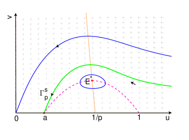
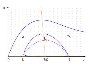
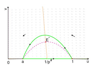
a) b) c) d)

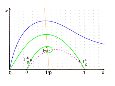
Figure 6: Phase portrait of (3) for $c<\dfrac{1}{r(1-a)}$ when a) $p_{H}<p<p^{\#}$ and close to $p_{H}$; b) $p_{H}<p<p^{\#}$ and close to $p^{\#}$; c) $p=p^{\#}$; d) $p^{\#}<p<\frac{1}{a}$.

Proof. If $a(p_{H})<0$, from theorem 2, stable periodic orbits bifurcating from Hopf bifurcation appear when $p>p_{H}$. According to proposition 8 (ii), if $p_{\#}<p_{H}$, there will be at least two distinct periodic orbits, which contradicts our assumption about the uniqueness of periodic orbit. Thus, we have $p_{H}\leq p_{\#}$. Since $E^{*}$ is asymptotically stable for any $1<p<p_{H}$, if there is a periodic orbit, it must be unstable from inside, which contradicts our assumption about the orbital stability of periodic orbit. Therefore, there is no periodic orbit when $1<p<p_{H}$, and the conclusion (i) follows from proposition 5 (i).

For the case of $p^{\#}<p<\frac{1}{a}$, any orbit must encircle $E^{*}$ and lie wholly in $\Omega_{1}$, which is negatively invariant by proposition 5 (ii). Thus, if there is a periodic orbit, it must be unstable from outside, which contradicts our assumption about the orbital stability of periodic orbit. Therefore, the conclusion (iv) follows from proposition 5 (ii). Moreover, together with the fact that Hopf bifurcating periodic orbit appears when $p>p_{H}$, the nonexistence of periodic orbits for $p^{\#}<p<\frac{1}{a}$ implies that $p_{H}$ is strictly less that $p_{\#}$.

If $p_{H}<p<p^{\#}$, $E^{*}$ is a repellor, thus it follows from proposition 6 (i) that there is a periodic orbit for all $p_{H}<p<p^{\#}$. Noticing that we have proved there is no cycle for $p>p^{\#}$, according to the work of Alexander JC ; Chow SN ; Wu J , the period of the unique cycle must tend to infinity as $p\rightarrow p^{\#}$. Proposition 5 (i) completes the proof of (ii).

When $p=p^{\#}$, then $p>p_{H}$, and $E^{*}$ is a repellor, from Poincaré-Bendixson theorem, the loop of heteroclicic orbits is the $\omega$-limit set of orbits through any point in its interior. $~{}~{}~{}~{}~{}~{}~{}~{}~{}~{}~{}~{}~{}~{}~{}~{}~{}~{}~{}~{}\Box$

      Remark 3.

From the former conclusion on the global dynamics of model (3) with weak cooperation, we find that no matter how we choose the value of $p$, both of the two species are extinct if the ratio of predator to prey is high.

Now we discuss the population behavior when the ratio of predator to prey is low. When $p<1$, because of the low conversion rate the predator is extinct, while the prey reach the capacity of the environment. When $1<p<p_{H}$, the predator and prey coexist, and tends to a stable value. When $p_{H}<p<p^{\#}$, the predator and prey coexist, but oscillate sustainably. The amplitude of oscillation increases as $p$ increases, and the minimum of the predator population is close to zero when $p$ is close to $p^{\#}$, which will increase of risk on the extinction of predator. When the value of $p$ is too high, high growth rate of prey leads to over hunting, and finally, both of the two species are extinct.

2.2 The system with strong cooperative hunting

By strong cooperation we mean $c>\frac{1}{r(1-a)}$. In this section, we first analyze the existence and stability of interior equilibrium, then we prove the existence of Hopf bifurcation and give the condition of the existence and nonexistence of loop of heteroclinic orbits. We also exhibit the complex dynamics of model (3), such as limit cycle, loop of heteroclinic orbits, and homoclinic cycle.

2.2.1 Existence and stability of equilibria

When $c>\frac{1}{r(1-a)}$, the existence and stability of the boundary equilibria are the same as the case of $c<\frac{1}{r(1-a)}$, which have been discussed in lemma 2. For interior equilibria, it is more complicated, and we have the following conclusion.

Proposition 9.

Suppose that $c>\frac{1}{r(1-a)}$.
       (i) When $p\geq\frac{1}{a}$, system (3) has no interior equilibria.
       (ii) When $1\leq p<\frac{1}{a}$, system (3) has a unique positive constant equilibrium $E^{*}(u^{*},v^{*})$.
       (iii) There exists a $p_{SN}<1$, such that system (3) has
       ($a$) two interior equilibria $E^{*}$ and $E^{*}_{R}$ when $p_{SN}<p<1$;
       (b) one interior equilibrium $E_{R}^{**}$ when $p=p_{SN}$; and
       (c) no interior equilibria when $p<p_{SN}$.

Proof. The proofs for $p\geq\frac{1}{a}$ and $1<p<\frac{1}{a}$ are the same as that of proposition 1. When $\frac{1}{p}$ increases to $1$, the $v-$nullcline $v=g(u)$ and $u-$nullcline $v=f(u)$ intersect at $E_{1}(1,0)$. The tangents of $v-$nullcline and $u-$nullcline at $E_{1}(1,0)$ are $-\frac{1}{c}$ and $-r(1-a)$ respectively. If $-\frac{1}{c}>-r(1-a)$, $E_{R}^{*}$ (sitting in the forth quadrant when $1<p<\frac{1}{a}$) collides with $E_{1}$ when $p=1$, and there is a unique interior equilibrium $E^{*}$ in the first quadrant (see Fig. 7 a)). When $p<1$ and close to $1$, $E_{R}^{*}$ moves into the first quadrant, and there are two interior equilibria $E^{*}$ and $E_{R}^{*}$ (see Fig. 7 b)). If $p<1$ goes on to decrease, there exists a $p_{SN}$, such that the $u-$nullcline $v=f(u)$ and $v-$nullcline $v=g(u)$ tangent at $E_{R}^{**}$, where $E^{*}$ and $E_{R}^{*}$ collide, and there is a unique interior equilibrium $E_{R}^{**}$ (see Fig. 7 c)). When $p<p_{SN}$, there is no interior equilibria (see Fig. 7 d)). $~{}~{}~{}~{}~{}~{}~{}~{}~{}~{}~{}~{}~{}~{}~{}~{}~{}~{}~{}~{}~{}~{}~{}~{}~{}~{}~{}~{}~{}~{}~{}~{}~{}~{}~{}~{}~{}~{}~{}~{}~{}~{}~{}~{}~{}~{}~{}~{}~{}~{}~{}~{}~{}~{}~{}~{}~{}~{}~{}~{}~{}~{}~{}~{}~{}~{}~{}~{}~{}~{}~{}~{}~{}~{}~{}~{}~{}~{}~{}~{}~{}~{}~{}~{}~{}~{}~{}~{}~{}~{}~{}~{}~{}~{}~{}~{}~{}~{}~{}~{}~{}~{}~{}~{}~{}~{}~{}~{}~{}~{}~{}~{}~{}~{}~{}~{}~{}~{}~{}~{}~{}~{}~{}~{}~{}~{}~{}~{}~{}~{}~{}~{}~{}~{}~{}~{}~{}~{}~{}~{}~{}~{}~{}~{}~{}~{}~{}~{}~{}~{}~{}~{}~{}~{}~{}~{}~{}~{}~{}~{}\Box$

      Remark 4.

In the absence of cooperative hunting within the predator, i.e., $c=0$, system (3) always has a unique interior equilibrium $E_{0}^{*}=(\frac{1}{p},r(1-\frac{1}{p})(\frac{1}{p}-a))$. The predator and prey coexists if and only if $1<p<\frac{1}{a}$, and the predator is distinct if $p<1$. However, from proposition 9, the predator and prey still coexist when $p_{SN}<p<1$ with strong cooperation, which means that strong cooperation is beneficial for the survival of predator.

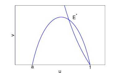
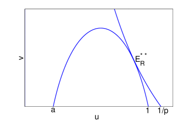
a) b)
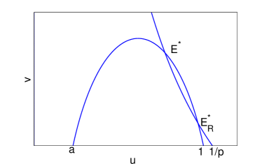
c) d)

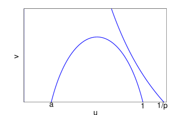
Figure 7: If $c>\dfrac{1}{r(1-a)}$, there is a) one interior equilibrium when $p=1$; b) two interior equilibria when $p_{SN}<p<1$; c) one equilibrium when $p=p_{SN}$; and d) no interior equilibria when $p<p_{SN}$.

Now we consider the stability of interior equilibria. For $E^{*}$ or $E_{R}^{*}$, the corresponding Jacobian matrix is

$$J=\left(\begin{array}[]{cc}ru(1+a-2u)&-2cuv-u\\ mpv(1+cv)&mpcuv\end{array}\right),$$ (8)

and thus

$$\begin{array}[]{l}{\rm tr}J=-ru(2u-a-1)+mpcuv=-ru(2u-a-1)+m(1-pu),\\ {\rm det}J=mpuv\left[rcu(1+a-2u)+(1+cv)(1+2cv)\right]=\frac{mv}{u}\left[rcpu^{3}(1+a-2u)+\frac{2}{p}-u\right].\end{array}$$

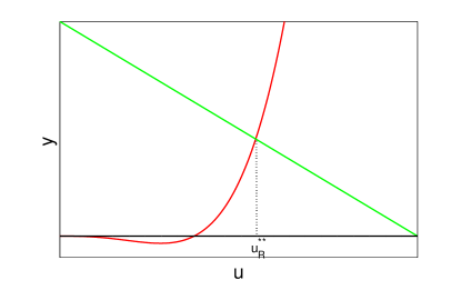
Figure 8: The red curve represents the figure of $y=rcpu^{3}(2u-a-1)$, and the green straight line represents for $y=2/p-u$.

If ${\rm det}J=0$, then $\frac{r(1+a-2u)}{1+2cv}=\frac{1+cv}{-cu}$, which means that $v=f(u)$ is tangent to $v=g(u)$. In fact, the point of tangency is $E_{R}^{**}$, thus ${\rm det}J_{E_{R}^{**}}=0$. It is clear that ${\rm det}J>0$ for $u<u_{R}^{**}$, and ${\rm det}J<0$ for $u>u_{R}^{**}$ (see Fig. 8). The component $u^{*}$ of $E^{*}$ is always satisfying $u^{*}<u_{R}^{**}$, and the component $u_{R}^{*}$ of $E_{R}^{*}$ is satisfying $u_{R}^{*}>u_{R}^{**}$ (see Fig. 7). It follows that for $E^{*}$, ${\rm det}J_{E^{*}}>0$, while for $E_{R}^{*}$, ${\rm det}J_{E_{R}^{*}}<0$. Thus, $E_{R}^{*}$ exists when $p_{SN}<p<1$, and it is a saddle. $E^{*}(u^{*},v^{*})$ exists when $p_{SN}<p<\frac{1}{a}$, and ${\rm det}J_{E^{*}}>0$. Thus, $E^{*}$ may be node or focus, and its stability depends on the trace

$${\rm tr}J_{E^{*}}=-ru^{*}(2u^{*}-a-1)+m(1-pu^{*}).$$ (9)

Similar as the proof in Theorem 1, solving for ${\rm tr}J_{E^{*}}=0$, when $\frac{a+1}{2}<\frac{1}{p}<\frac{1}{p_{SN}}$, there is a unique $u_{H}^{*}\in(\frac{a+1}{2},\frac{1}{p_{SN}})$ such that ${\rm tr}J_{E^{*}}>0$ on $(0,u_{H}^{*})$, and ${\rm tr}J_{E^{*}}<0$ on $(u_{H}^{*},\frac{1}{p_{SN}})$ (see Fig. 3). Recalling that $\frac{\partial u^{*}}{\partial p}<0$, corresponding to $u_{H}^{*}$, we obtain a unique $p_{H}$ ($p_{SN}<p_{H}<\frac{2}{a+1}$), such that ${\rm tr}J_{E^{*}}>0$ when $p\in(p_{H},\frac{1}{a})$, and ${\rm tr}J_{E^{*}}<0$ when $p\in(p_{SN},p_{H})$.

Let $\mu=\alpha(p)\pm i\omega(p)$ be the roots of $\mu^{2}-{\rm tr}J_{E^{*}}\mu+{\rm det}J_{E^{*}}=0$ when $p$ is near $p_{H}$. We can prove $\alpha^{\prime}(p)\mid_{p=p_{H}}>0$, in a similar way as in Theorem 1. Therefore, we can get the following theorem.

      Theorem 5.

When $c>\frac{1}{r(1-a)}$, there exists a unique $p_{H}\in(p_{SN},\frac{2}{a+1})$ such that $E^{*}$ is locally asymptotically stable if $p_{SN}<p<p_{H}$, and unstable if $p_{H}<p<\frac{1}{a}$. Moreover, system (3) undergoes a Hopf bifurcation at $E^{*}$ when $p=p_{H}$.

2.2.2 The global dynamics of system (3) with strong cooperative hunting

When $c>\frac{1}{r(1-a)}$, system (3) may have one or two interior equilibria, which brings a few complications to the dynamics of model (3). There are three different cases of global dynamics when $c$ takes different sizes. In this section, we exhibit the dynamics combining theoretical analysis and numerical simulations.

Firstly, we consider the properties of the stable manifold of $E_{a}$ and unstable manifold of $E_{1}$, denoted by $\Gamma_{p}^{s}(E_{a})$ and $\Gamma_{p}^{u}(E_{1})$, respectively.

Proposition 10.

Suppose that $c>\frac{1}{r(1-a)}$, and $p_{SN}<p<\frac{1}{a}$.
       (i) The orbit $\Gamma_{p}^{s}(E_{a})$ meets the $v-$nullcline $v=g(u)$ at a point $(u_{p}^{s},S_{a}(p))$, where $S_{a}(p)\geq v^{*}:=f(u^{*})$, and $S_{a}(p)$ is a monotone decreasing function for $p\in(p_{SN},\frac{1}{a})$.
       (ii) The orbit $\Gamma_{p}^{u}(E_{1})$ meets the $v-$nullcline $v=g(u)$ at a point $(u_{p}^{u},U_{1}(p))$, where $U_{1}(p)\geq v^{*}:=f(u^{*})$, and $U_{1}(p)$ is a monotone increasing function for $p\in(1,\frac{1}{a})$.

Proof. The proof is similar as in proposition 3.

      Theorem 6.

Suppose that $c>\frac{1}{r(1-a)}$.
       (i) If $U_{1}(1^{+})<S_{a}(1^{+})$, there exists a unique $p^{\#}\in(1,\frac{1}{a})$, such that $\Gamma_{p^{\#}}^{s}(E_{a})=\Gamma_{p^{\#}}^{u}(E_{1})$, forming a heteroclinic orbit from $E_{1}$ to $E_{a}$;
       (ii) If $U_{1}(1^{+})>S_{a}(1^{+})$, $\Gamma_{p}^{s}(E_{a})\neq\Gamma_{p}^{u}(E_{1})$ for any $p\in(0,+\infty)$.

Proof. (i) If $U_{1}(1^{+})<S_{a}(1^{+})$, then

$$\lim_{p\rightarrow\frac{1}{a}^{-}}(S_{a}(p)-U_{1}(p))<0,{\rm and}\lim_{p\rightarrow 1^{+}}(S_{a}(p)-U_{1}(p))>0.$$

From the monotonicity of $S_{a}(p)$ and $U_{1}(p)$, there exists a unique $p^{\#}$ such that $S_{a}(p^{\#})=U_{1}(p^{\#})$.

(ii) If $U_{1}(1^{+})>S_{a}(1^{+})$, from the monotonicity of $S_{a}(p)$ and $U_{1}(p)$, $U_{1}(p)>S_{a}(p)$ for any $p\in(1,\frac{1}{a})$. Noticing that $E_{1}$ becomes a stable node when $p<1$ and $E_{a}$ is an unstable node if $p>\frac{1}{a}$, there is no $p^{\#}$, such that $\Gamma_{p^{\#}}^{s}(E_{a})=\Gamma_{p^{\#}}^{u}(E_{1})$. $~{}~{}~{}~{}~{}~{}~{}~{}~{}~{}~{}~{}~{}~{}~{}~{}~{}~{}~{}~{}~{}~{}~{}~{}~{}~{}\Box$

In fact, the unstable manifold of $E_{a}$ on the $u-$axis connects $E_{a}$ to $E_{1}$, which is another heteroclinic orbit. Then, if $U_{1}(1^{+})<S_{a}(1^{+})$, there is a loop of heteroclinic orbits from $E_{1}$ to $E_{a}$, and then back to $E_{1}$. If $U_{1}(1^{+})>S_{a}(1^{+})$, such a loop of heteroclinic orbits does not exist.

Let $\Omega_{21}$ denotes the bounded open subset of the positive quadrant, boundary with $\Gamma_{p}^{s}(E_{a})$, $v-$nullcline between $\Gamma_{p}^{s}(E_{a})$ and $\Gamma_{p}^{u}(E_{1})$, $\Gamma_{p}^{u}(E_{1})$, and the segment from $E_{1}$ to $E_{a}$ on the $u-$axis.

Proposition 11.

Suppose that $c>\frac{1}{r(1-a)}$, and $1<p<\frac{1}{a}$.
       (i) Assume $U_{1}(1^{+})<S_{a}(1^{+})$.
       (a) If $1<p<p^{\#}$, $S_{a}(p)>U_{1}(p)$. All orbits in the positive quadrant above $\Gamma_{p}^{s}(E_{a})$ converge to $E_{0}$. All orbits below $\Gamma_{p}^{s}(E_{a})$ have their $\omega-$limit sets in $\Omega_{21}$, which is a positive invariant set.
       (b) If $p^{\#}<p<\frac{1}{a}$, $S_{a}(p)<U_{1}(p)$, and $\Gamma_{p}^{u}(E_{1})$ enters $E_{0}$. All orbits in the positive quadrant above $\Gamma_{p}^{u}(E_{1})$ converge to $E_{0}$. All orbits below $\Gamma_{p}^{u}(E_{1})$ have their $\alpha-$limit sets in $\Omega_{21}$, which is a negative invariant set.
      (ii) Assume $U_{1}(1^{+})>S_{a}(1^{+})$. $S_{a}(p)<U_{1}(p)$ for all $p\in(1,\frac{1}{a})$, and $\Gamma_{p}^{u}(E_{1})$ enters $E_{0}$. All orbits in the positive quadrant above $\Gamma_{p}^{u}(E_{1})$ converge to $E_{0}$. All orbits below $\Gamma_{p}^{u}(E_{1})$ have their $\alpha-$limit sets in $\Omega_{21}$, which is a negative invariant set.

Proof. The proof is similar as proposition 5. $~{}~{}~{}~{}~{}~{}~{}~{}~{}~{}~{}~{}~{}~{}~{}~{}~{}~{}~{}~{}~{}~{}~{}~{}~{}~{}~{}~{}~{}~{}~{}~{}~{}~{}~{}~{}~{}~{}~{}~{}~{}~{}~{}~{}~{}~{}~{}~{}~{}~{}~{}~{}~{}~{}~{}~{}~{}~{}~{}~{}~{}~{}~{}~{}~{}~{}~{}~{}~{}~{}~{}~{}~{}~{}~{}~{}~{}~{}~{}~{}~{}~{}\Box$

If $c>\frac{1}{r(1-a)}$, $E_{R}^{*}$ exists when $p_{SN}<p<1$, and it is a saddle. Now we consider the properties of the stable manifold and unstable manifold of $E_{R}^{*}$, denoted by $\Gamma_{p}^{s}(E_{R}^{*})$ and $\Gamma_{p}^{u}(E_{R}^{*})$, respectively.

Proposition 12.

Suppose that $c>\frac{1}{r(1-a)}$, and $p_{SN}<p<1$. The downward unstable manifold $\Gamma_{p}^{u}(E_{R}^{*})$ connects $E_{1}$. The right stable manifold $\Gamma_{p}^{s}(E_{R}^{*})$ enters $E_{R}^{*}$ from the lower right.
       (i) The orbit of left $\Gamma_{p}^{s}(E_{R}^{*})$ meets the $v-$nullcline $v=g(u)$ at a point $(u_{p}^{s},S_{R}(p))$, where $S_{R}(p)\geq v^{*}:=f(u^{*})$.
       (ii) The orbit of upward $\Gamma_{p}^{u}(E_{R}^{*})$ meets the $v-$nullcline $v=g(u)$ at a point $(u_{p}^{u},U_{R}(p))$, where $U_{R}(p)\geq v^{*}:=f(u^{*})$.

Proof. For the negative eigenvalue $\lambda_{1}$ of the Jacobian of $E_{R}^{*}$, the corresponding eigenvector is $(1,\frac{mpv(1+cv)}{-mpcuv+\lambda_{1}})$. Noticing that the tangent vector of $v=g(u)$ at $E_{R}^{*}$ is $\frac{mpv(1+cv)}{-mpcuv}$, the left part of $\Gamma_{p}^{s}(E_{R}^{*})$ near $E_{R}^{*}$ is below the $v-$nullcline, and the right part of $\Gamma_{p}^{s}(E_{R}^{*})$ near $E_{R}^{*}$ is above the $v-$nullcline. Obviously, the right part of $\Gamma_{p}^{s}(E_{R}^{*})$ enters $E_{R}^{*}$ from the lower right. From the vector field for (3), before the left part of $\Gamma_{p}^{s}(E_{R}^{*})$ meets the $v-$nullcline, the curve under the $u-$nullcline directs lower right; the curve above the $u-$nullcline directs lower left. Since it can not cross the stable manifold $\Gamma_{p}^{s}(E_{a})$, thus, it is bounded before it meets the $v-$nullcline. Thus the left part of $\Gamma_{p}^{s}(E_{R}^{*})$ must meet the $v-$nullcline at a point, denoted by $(u_{p}^{s},S_{R}(p))$. Obviously, $S_{R}(p)\geq v^{*}$.

(ii) can be proved similarly. $~{}~{}~{}~{}~{}~{}~{}~{}~{}~{}~{}~{}~{}~{}~{}~{}~{}~{}~{}~{}~{}~{}~{}~{}~{}~{}~{}~{}~{}~{}~{}~{}~{}~{}~{}~{}~{}~{}~{}~{}~{}~{}~{}~{}~{}~{}~{}~{}~{}~{}~{}~{}~{}\Box$

Let $\Omega_{22}$ denotes the bounded open subset of the positive quadrant, boundary with the left $\Gamma_{p}^{s}(E_{R}^{*})$, $v-$nullcline between $\Gamma_{p}^{s}(E_{R}^{*})$ and $\Gamma_{p}^{u}(E_{R}^{*})$, upward $\Gamma_{p}^{u}(E_{R}^{*})$. Similar as proposition 11, we have the following conclusion.

Proposition 13.

       (i) If $S_{R}(p)>U_{R}(p)$. All orbits inside the region boundary with $\Gamma_{p}^{s}(E_{R}^{*})$ have their $\omega-$limit sets in $\Omega_{22}$, which is a positive invariant set.
       (ii) If $S_{R}(p)<U_{R}(p)$. All orbits below the left $\Gamma_{p}^{u}(E_{R}^{*})$ have their $\alpha-$limit sets in $\Omega_{22}$, which is a negative invariant set.

From the previous discussion, we can determine the global dynamics of model (3) when $p$ is chosen in the following ranges. Similar as in Theorem 3, we can prove the following conclusion.

      Theorem 7.

Suppose that $c>\frac{1}{r(1-a)}$.
       (i) If $p\geq\frac{1}{a}$, $E_{0}(0,0)$ is globally asymptotically stable (see Fig. 9 a)).
       (ii) If $p<\frac{1}{a}$ and near $\frac{1}{a}$, $\Gamma_{p}^{s}(E_{a})$ connects $E^{*}$ to $E_{a}$, and the extinction equilibrium $E_{0}(0,0)$ is globally asymptotically stable (see Fig. 9 b) ).
       (iii) If $p<p_{SN}$, the orbits through any point above $\Gamma_{p}^{s}(E_{a})$ converge to $E_{0}$, and the orbits through any point below $\Gamma_{p}^{s}(E_{a})$ converge to $E_{1}$ (see Fig. 9 c)).

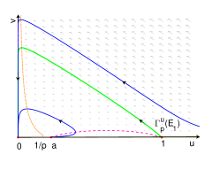
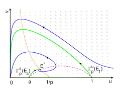
a) b) c)

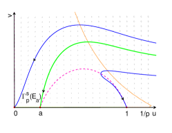
Figure 9: If $c>\frac{1}{r(1-a)}$, phase portrait of (3) when a) $p\geq\dfrac{1}{a}$; b) $p<\dfrac{1}{a}$ and close to $\dfrac{1}{a}$; and c) $p<p_{SN}$.

The remaining question is how are the dynamics of system (3) for $p$ chosen in the rest ranges, i.e., $p_{SN}<p<\frac{1}{a}$. Since larger $c$ means less steep of the $v-$nullcline, the critical points (for example $p_{H}$, $p^{\#}$) may appear in different ranges, and there are the following three different cases.

Case 1 Choose suitable $c$ such that $c>\frac{1}{r(1-a)}$, $U_{1}(1^{+})<S_{a}(1^{+})$, and $p_{H}>1$. From theorem 6, there is a loop of heteroclinic orbits when $p=p^{\#}$. We have the following conclusion.

      Theorem 8.

Suppose that $c>\frac{1}{r(1-a)}$, $U_{1}(1^{+})<S_{a}(1^{+})$, and $p_{H}>1$. Assume that the first Lyapunov coefficient $a(p_{H})<0$, and every periodic orbit of system (3) is orbitally stable, then $p_{H}<p^{\#}$.
      (i) If $p_{SN}<p<1$, the upward $\Gamma_{p}^{u}(E_{R}^{*})$ connects $E_{R}^{*}$ to $E^{*}$. The orbits through any point above $\Gamma_{p}^{s}(E_{a})$ converge to $E_{0}$, and the orbits through any point inside the stable manifold $\Gamma_{p}^{s}(E_{R}^{*})$ converge to $E^{*}$. The orbits through any point below $\Gamma_{p}^{s}(E_{a})$ and exterior to $\Gamma_{p}^{s}(E_{R}^{*})$ converge to $E_{1}$ (see Fig. 10 a) ).
      (ii) If $1<p<p_{H}$, $\Gamma_{p}^{u}(E_{1})$ connects $E_{1}$ to $E^{*}$. The orbits through any point above $\Gamma_{p}^{s}(E_{a})$ converge to $E_{0}$, and the orbits through any point below $\Gamma_{p}^{s}(E_{a})$ converge to $E^{*}$.
      (iii) When $p_{H}<p<p^{\#}$, $E^{*}$ is a repellor, and there is a unique limit cycle under $\Gamma_{p}^{s}(E_{a})$. The orbits through any point below $\Gamma_{p}^{s}(E_{a})$ converge to the limit cycle. (see Fig. 10 b), c)).
       (iv) When $p=p^{\#}$, $\Gamma_{p^{\#}}^{s}(E_{a})=\Gamma_{p^{\#}}^{u}(E_{1})$, and there are two heteroclinic orbits forming a loop of heteroclinic orbits between $E_{1}$ and $E_{a}$ (see Fig. 10 d)). The orbits through any point exterior to the cycle converge to $E_{0}$, and the orbits through any point interior to the cycle converge to the cycle.
      (v) If $p^{\#}<p<\frac{1}{a}$, $\Gamma_{p}^{s}$ connects $E^{*}$ to $E_{a}$, and the extinction equilibrium $E_{0}(0,0)$ is globally asymptotically stable (phase portrait is similar as Fig. 9 b)).

Proof. From proposition 10, $S_{a}(p)$ is decreasing with $p$, combining with $U_{1}(1^{+})<S_{a}(1^{+})$, then $\Gamma_{p}^{s}(E_{a})$ enters $E_{a}$ from the region $\{(u,v):v>f(u)\}$ for all $p<1$. Since $E^{*}$ is stable when $p<p_{H}$, then $E^{*}$ is stable for all $p_{SN}<p<1$. If there is a periodic orbit below $\Gamma_{p}^{s}(E_{a})$, it must encircle $E^{*}$, and it is unstable from inside, which contradicts with our assumption of the orbital stability of periodic orbit. It means that there is no periodic orbit under $\Gamma_{p}^{s}(E_{a})$ for all $p<1$. From proposition 13, $E^{*}$ is the $\omega-$limit set of $\Omega_{22}$, and $\Gamma_{p}^{s}(E_{R}^{*})$ must be above $\Gamma_{p}^{u}(E_{R}^{*})$. The upward $\Gamma_{p}^{u}(E_{R}^{*})$ connects $E_{R}^{*}$ to $E^{*}$ (see Fig. 10 a) ). Thus, the orbits through any point inside the stable manifold $\Gamma_{p}^{s}(E_{R}^{*})$ converge to $E^{*}$. The proof of (ii)-(v) is similar as that of theorem 4. $~{}~{}~{}~{}~{}~{}~{}~{}~{}~{}~{}~{}~{}~{}~{}~{}~{}~{}~{}~{}~{}~{}~{}~{}~{}~{}~{}~{}~{}~{}~{}~{}~{}~{}~{}~{}~{}~{}~{}~{}~{}~{}~{}~{}~{}~{}~{}~{}~{}~{}~{}~{}~{}~{}~{}~{}~{}~{}~{}~{}~{}~{}~{}~{}~{}~{}~{}~{}~{}~{}~{}~{}~{}~{}~{}~{}~{}~{}~{}~{}~{}~{}~{}~{}~{}~{}~{}~{}~{}~{}~{}~{}~{}~{}~{}~{}~{}~{}~{}~{}~{}~{}~{}~{}~{}~{}~{}~{}~{}~{}~{}~{}~{}~{}~{}~{}~{}~{}~{}~{}~{}~{}~{}~{}~{}~{}~{}~{}~{}~{}~{}~{}~{}~{}~{}~{}~{}~{}~{}~{}~{}~{}~{}~{}~{}~{}~{}~{}~{}~{}~{}~{}~{}~{}~{}~{}~{}\Box$

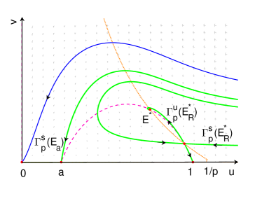
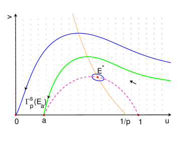
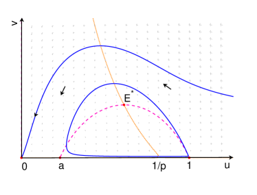
a)b) c) d)

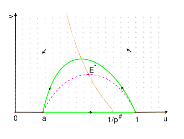
Figure 10: Phase portrait of system (3) for case $1$ when a) $p>p_{SN}$ and close to $p_{SN}$; b) $p>p_{H}$ and close to $p_{H}$; c) $p_{H}<p<p^{\#}$ and close to $p^{\#}$; and d) $p=p^{\#}$.

Case 2 Choose suitable $c$ such that $c>\frac{1}{r(1-a)}$, $U_{1}(1^{+})<S_{a}(1^{+})$, and $p_{H}<1$. From Theorem 6, there is a loop of heteroclinic orbits when $p=p^{\#}$.

      Theorem 9.

Choose suitable $c$ such that $c>\frac{1}{r(1-a)}$, $U_{1}(1^{+})<S_{a}(1^{+})$, and $p_{H}<1$. Assume that the first Lyapunov coefficient $a(p_{H})<0$, and every periodic orbit of system (3) is orbitally stable, then $p_{H}<p^{\#}$.
       (i) If $p_{SN}<p<p_{H}$, the upward $\Gamma_{p}^{u}(E_{R}^{*})$ connects $E_{R}^{*}$ to $E^{*}$, and the downward $\Gamma_{p}^{u}(E_{R}^{*})$ connects $E_{R}^{*}$ to $E_{1}$. The orbits through any point above $\Gamma_{p}^{s}(E_{a})$ converge to $E_{0}$, and the orbits through any point inside the stable manifold $\Gamma_{p}^{s}(E_{R}^{*})$ converge to $E^{*}$. The orbits through any point below $\Gamma_{p}^{s}(E_{a})$ and exterior to $\Gamma_{p}^{s}(E_{R}^{*})$ converge to $E_{1}$ (phase portrait is similar as Fig. 10 a) ).
       (ii) When $p_{H}<p<1$, there is a unique limit cycle inside the stable manifold $\Gamma_{p}^{s}(E_{R}^{*})$ of $E_{R}^{*}$. (see Fig. 11 a) ). The orbits through any point interior to $\Gamma_{p}^{s}(E_{R}^{*})$ converge to the limit cycle.
       (iii) When $1<p<p^{\#}$, there is a unique limit cycle under $\Gamma_{p}^{s}$. The orbits through any point below $\Gamma_{p}^{s}$ converge to the limit cycle. (see Fig. 11 b) ).
       (iv) When $p=p^{\#}$, $\Gamma_{p^{\#}}^{s}(E_{a})=\Gamma_{p^{\#}}^{u}(E_{1})$, there are two heteroclinic orbits forming a loop of heteroclinic orbits from $E_{1}$ to $E_{a}$ and back to $E_{1}$ (see Fig. 11 c)). The orbits through any point exterior to the cycle converge to $E_{0}$, and the orbits through any point interior to the cycle converge to the cycle.
      (v) If $p^{\#}<p<\frac{1}{a}$, $\Gamma_{p}^{s}$ connects $E^{*}$ to $E_{a}$, and the extinction equilibrium $E_{0}(0,0)$ is globally asymptotically stable (phase portrait is similar as Fig. 9 b)).

Proof. We can prove (i) similar as in Theorem 8. (ii) Since $a(p_{H})<0$ and $\alpha^{\prime}(p_{H})>0$, there is a stable periodic orbit bifurcating from Hopf bifurcation when $p>p_{H}$. Similar as the proof in Theorem 8, we can prove that $\Gamma_{p}^{s}(E_{R}^{*})$ must be above $\Gamma_{p}^{u}(E_{R}^{*})$. From proposition 13, the unique limit cycle is the $\omega-$limit set of $\Omega_{22}$. The proof of (iii)-(v) is similar as that of Theorem 4. $~{}~{}~{}~{}~{}~{}~{}~{}~{}~{}~{}~{}~{}~{}~{}~{}~{}~{}~{}~{}~{}~{}~{}~{}~{}~{}~{}~{}~{}~{}~{}~{}~{}~{}~{}~{}~{}~{}~{}~{}~{}~{}~{}~{}~{}~{}~{}~{}~{}~{}~{}~{}~{}~{}~{}~{}~{}~{}~{}~{}~{}~{}~{}~{}~{}~{}~{}~{}~{}~{}~{}~{}~{}~{}~{}~{}~{}~{}~{}~{}~{}\Box$

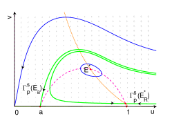
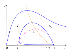
a) b) c)

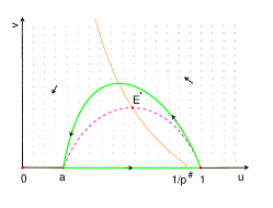
Figure 11: Phase portrait of system (3) for case $2$ when a) $p_{H}<p<1$ and close to $p_{H}$; b) $p_{H}<p<p^{\#}$ and close to $p^{\#}$; c) $p=p^{\#}$.

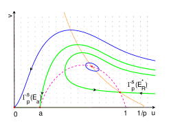
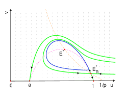
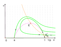
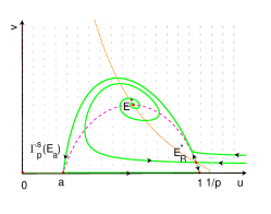
a) b) c) d) e)

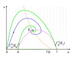
Figure 12: Phase portrait of system (3) for case $3$ when a) When $p>p_{H}$ and near $p_{H}$, there is a limit cycle inside the stable manifold of $E_{R}^{*}$; b) When $p<p_{hom}$ and near $p_{hom}$, there is a limit cycle inside the stable manifold of $E_{R}^{*}$; c) When $p=p_{hom}$, the upward unstable manifold and the left stable manifold of $E_{R}^{*}$ collide, which forms a homoclinic cycle; d) The upward unstable manifold of $E_{R}^{*}$, the unstable manifold of $E_{a}$ on the $u-$axis, and the downward unstable manifold of $E_{R}^{*}$ forms a loop of heteroclinic orbits among $E_{R}^{*}$, $E_{a}$ and $E_{1}$ when $p=\overline{p}^{\#}$; e) $1<p<\frac{1}{a}$.

Case 3 Choose $c$ such that $c>\frac{1}{r(1-a)}$ and $U_{1}(1^{+})>S_{a}(1^{+})$. From Theorem 6, there is no heteroclinic orbits from $E_{1}$ to $E_{a}$. It is easy to prove that when $1<p<\frac{1}{a}$, $E_{0}$ is globally asymptotically stable (see Fig. 12 e)).

      Remark 5.

In this case, the location of $\Gamma_{p}^{s}(E_{a})$, $\Gamma_{p}^{s}(E_{R}^{*})$ and $\Gamma_{p}^{u}(E_{R}^{*})$ are very complicated. We can observe the following dynamics by numerical simulations. (i) Loop of heteroclinic orbits. The downward branch of the unstable manifold of $E_{R}^{*}$ connects $E_{R}^{*}$ to $E_{1}$, and the upward connects $E_{R}^{*}$ to $E_{a}$, which collides with the the stable manifold of $E_{a}$. The upward and downward unstable manifold of $E_{R}^{*}$, together with the unstable manifold of $E_{a}$ on the $u-$ axis, forms a loop of heteroclinic orbits among $E_{R}^{*}$, $E_{a}$ and $E_{1}$ when $p=\overline{p}^{\#}$ (see Fig. 12 d)). (ii) Homoclinic cycle. The upward unstable manifold and the left stable manifold of $E_{R}^{*}$ collide, which forms a homoclinic cycle. Denote the parameter $p$ as $p=p_{hom}$ (see Fig. 12 c)). (iii) Limit cycle induced by Hopf bifurcation (see Fig. 12 a), b)).

2.3 Numerical simulations for ODE system

In this section, we carry out some mumerical simulations for system (3). We fix the parameters as

$$a=0.23,r=1.1,m=0.31.$$ (10)

2.3.1 Numerical simulations for system (3) with weak cooperative hunting

For system (3), choose $c=0.25$ such that $c<\frac{1}{r(1-a)}$, and vary the parameter $p$. Using the method in Dhooge A , we can get Hopf bifurcation point $p_{H}=1.5432$, and the first Lyapunov coefficient is $-1.1211$, which means that the bifurcating periodic solution is asymptotically stable, and it is bifurcating from $E^{*}$ as $p$ increases past $p_{H}$ from Theorem 2. We can also draw the bifurcation diagram in Fig. 13, which shows that as $p$ increases from $p_{H}$, the period of limit cycle is increasing, and it tends to infinite as $p\rightarrow 1.6491$. Moreover, the amplitude of oscillation increases as $p$ increases, and the minimum of the predator population is close to zero when $p$ is close to $p^{\#}=1.6491$, which will increase the risk on the extinction of predator.

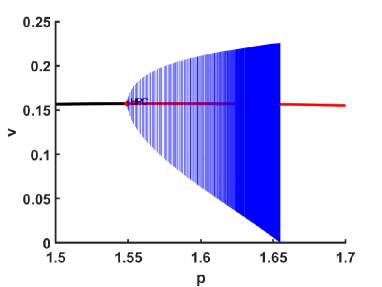
a) b)

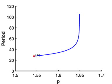
Figure 13: The bifurcation diagram with $a=0.23,m=0.31,r=1.1$ and $c=0.25$, and the conversion rate $p$ as the bifurcation parameter. a) The black curve is the stable steady state and the red curve is the unstable steady state. The blue curves denote the $v-$amplitude of the periodic orbits, which begin at the Hopf bifurcation point $p=p_{H}=1.5432$. b) The period of the limit cycles.

To show the complex dynamics of system (3), different values of $p$ are chosen, listed in Table 2. The corresponding phase portraits for different values of $p$ have been illustrated in Figs. 5 and 6, which is drawn by pplane8 Polking JA .

Table 2: Values of parameter $p$ chosen in Figs. 5 and 6

Figure	Fig. 5 a	Fig. 5 b	Fig. 5 c	Fig. 5 d	Fig. 6 a	Fig. 6 b	Fig. 6 c	Fig. 6 d
$p$	5.1	3.2	1.2	0.9	1.55	1.645	1.6491	1.95

2.3.2 Numerical simulations for ODE system with strong cooperative hunting

In section 2.2, we discuss three different cases of dynamics when $c$ is chosen as different values. To show case $1$, we fix $c=3$, and vary $p$ as a bifurcation parameter. We get $p_{H}=1.1024$, and the first Lyapunov coefficient is $-2.3280$. Choosing different values of $p$ listed in Table 3, we have drawn the corresponding phase portraits for different values of $p$ in Fig. 10.

Table 3: Values of parameter $p$ chosen for showing case $1$ in Figs. 10 and 11

Figure	Fig. 10 a	Fig. 10 b	Fig. 10 c	Fig. 10 d
$p$	0.96	1.105	1.2	1.2068
Figure	Fig. 11 a	Fig. 11 b	Fig. 11 c
$p$	0.965	1.052	1.05665

To show case $2$, we choose $c=5$, and vary $p$, we can get $p_{H}=0.9608$, and the first Lyapunov coefficient is $-2.9553$. Choosing $p$ as listed in Table 3, the corresponding phase portraits have been illustrated in Fig. 11.

To show case $3$, we choose $c=8$, and vary $p$, we can get $p_{H}=0.8306$, and the first Lyapunov coefficient is $-3.732$. We can draw the bifurcation diagram in Fig. 14, in which the curve above is the $v-$value of interior equilibrium $E^{*}$, and the curve below is the $v-$value of $E_{R}^{*}$. We can see that as $p$ increasing from $p_{H}$, the period of limit cycle is increasing, and it tends to infinite as $p\rightarrow 0.8919$. Moreover, the amplitude of oscillation increases as $p$ increases, and the amplitude line touches the curve of $v-$value of $E_{R}^{*}$, which means that there is a cycle goes through $E_{R}^{*}$. In fact, there is a homoclinic cycle when $p=p_{hom}=0.8919$ (see Fig. 12 c)). Choosing $p$ as listed in Table 4, the corresponding phase portraits have been illustrated in Fig. 12.

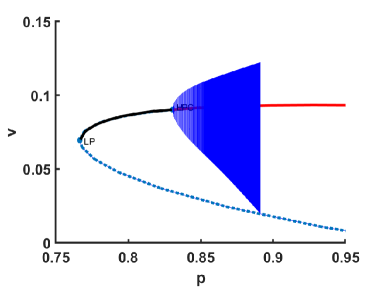
a) b)

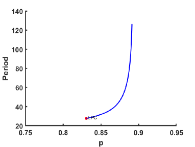
Figure 14: The bifurcation diagram with $a=0.23,m=0.31,r=1.1$ and $c=8$, and the conversion rate $p$ as the bifurcation parameter. a) The black curve is the stable steady state $E^{*}$, the red curve is the unstable steady state $E^{*}$, and the dotted blue curve is the unstable steady state $E_{R}^{*}$. The blue curves denote the $v-$amplitude of the periodic orbits, which begin at the Hopf bifurcation point $p=p_{H}=0.8306$. b) The period of the limit cycles.

Table 4: Values of parameter $p$ chosen for showing case $3$ in Fig. 12

Figure	Fig. 12 a	Fig. 12 b	Fig. 12 c	Fig. 12 d	Fig. 12 e
$p$	0.834	0.88	0.8919	0.91564	1.1

3 Diffusion-driven Turing instability and Turing-Hopf bifurcation

In the previous section, we have discussed both local and global dynamics of ODE model (3). In fact, the preys and predators distribute inhomogeneously in different locations, and the spatial diffusion plays an important part in the process of population evolution. Turing instability and Turing-Hopf bifurcation induced by diffusion have been widely investigated recently (see YongliSongTuringHopf ; X. Xu ; Q. An ; guogaihui ). Taking into account the diffusion in system (3), we consider the following diffusive predator-prey system:

$$\left\{\begin{array}[]{l}\dfrac{\partial u(x,t)}{\partial t}=d_{1}\Delta u(x,t)+ru(x,t)[1-u(x,t)](u(x,t)-a),\\ ~{}~{}~{}~{}~{}~{}~{}~{}~{}~{}~{}-(1+cv(x,t))u(x,t)v(x,t),~{}~{}~{}~{}~{}~{}~{}~{}~{}~{}~{}~{}~{}~{}~{}~{}~{}~{}~{}~{}~{}~{}~{}~{}~{}~{}~{}~{}~{}~{}~{}~{}~{}~{}~{}~{}~{}~{}~{}~{}~{}~{}~{}~{}~{}~{}~{}~{}~{}~{}~{}~{}x\in(0,l\pi),\\ \dfrac{\partial v(x,t)}{\partial t}=d_{2}\Delta v(x,t)+mv(x,t)\left[pu(x,t)\left(1+cv(x,t)\right)-1\right],~{}x\in(0,l\pi)\\ \partial_{x}u(x,t)=0,~{}~{}\partial_{x}v(x,t)=0,~{}~{}~{}~{}~{}~{}~{}~{}~{}~{}~{}~{}~{}~{}~{}~{}~{}~{}~{}~{}~{}~{}~{}~{}~{}~{}~{}~{}~{}~{}~{}~{}~{}~{}~{}~{}~{}~{}~{}~{}~{}~{}~{}~{}~{}~{}~{}~{}~{}~{}~{}~{}~{}~{}~{}~{}~{}~{}~{}~{}~{}~{}~{}~{}x=0,l\pi,\\ \end{array}\right.$$ (11)

where $d_{1},d_{2}>0$ are the diffusion coefficients characterizing the rates of the spatial dispersion of the prey and predator population, respectively.

3.1 Turing instability and Turing-Hopf bifurcation induced by diffusion

In this subsection, we consider the effect of the diffusion on the stability of the constant steady state $E^{*}$. If $E^{*}$ is linearly stable in the absence of diffusion, and it becomes unstable in the presence of diffusion, we call such an instability Turing instability. Since $E_{R}^{*}$ is always a saddle if it exists, thus Turing instability can only happen near $E^{*}$ in both cases: weak cooperation and strong cooperation. We first investigate the existence of Turing instability, then we consider Turing-Hopf bifurcation near $E^{*}$.

For Neumann boundary condition, we define the real-valued Sobolev space

$$X=\{(u,v)^{T}\in H^{2}(0,l\pi)\times H^{2}(0,l\pi),~{}\dfrac{\partial u}{\partial x}=\dfrac{\partial v}{\partial x}=0,{\rm at}~{}x=0,l\pi\}.$$ (12)

The linearization of system (11) at the constant steady state $E^{*}(u^{*},v^{*})$ is given by

$$\left(\begin{array}[]{c}\frac{\partial u}{\partial t}\\ \frac{\partial v}{\partial t}\end{array}\right)=D\left(\begin{array}[]{ c}\Delta u\\ \Delta v\end{array}\right)+A\left(\begin{array}[]{ c}u\\ v\end{array}\right)\stackrel{{\scriptstyle\vartriangle}}{{=}}L\left(\begin{array}[]{ c}u\\ v\end{array}\right),$$ (13)

where

$$D=\left(\begin{array}[]{ cc}d_{1}&0\\ 0&d_{2}\end{array}\right),~{}A=\left(\begin{array}[]{cc}ru^{*}(1+a-2u^{*})&-2cu^{*}v^{*}-u^{*}\\ mp(1+cv^{*})v^{*}&mpcu^{*}v^{*}\\ \end{array}\right).$$

It is well known that the eigenvalues of $D\Delta$ on $X$ are $-d_{1}\frac{n^{2}}{l^{2}}$ and $-d_{2}\frac{n^{2}}{l^{2}}$, $k\in\mathbb{N}_{0}=\{0,1,2,...\}$, with corresponding normalized eigenfunctions $\beta_{n}^{(1)}$ and $\beta_{n}^{(2)}$, where

$$\beta_{n}^{(1)}(x)=\left(\begin{array}[]{c }\gamma_{n}\\ 0\end{array}\right),~{}~{}\beta_{n}^{(2)}(x)=\left(\begin{array}[]{c }0\\ \gamma_{n}\end{array}\right),~{}~{}\gamma_{n}(x)=\dfrac{\cos\frac{n}{l}x}{\parallel\cos\frac{n}{l}x\parallel_{L^{2}}}=\left\{\begin{array}[]{ll}\sqrt{\frac{1}{l\pi}},&n=0,\\ \sqrt{\frac{2}{l\pi}}\cos\frac{n}{l}x,&n\geq 1.\end{array}\right.$$

Applying the general theory about elliptic operators, we know that $\beta_{n}^{(1)}$ and $\beta_{n}^{(2)}$ form an orthonormal basis for $X$.

From straightward calculation, we obtain the characteidtic equations

$$\Delta_{n}=\lambda^{2}-T_{n}\lambda+J_{n}=0,~{}~{}~{}~{}~{}~{}~{}n=0,1,2,...,$$ (14)

where

$$T_{n}=-\left(d_{1}\frac{n^{2}}{l^{2}}+d_{2}\frac{n^{2}}{l^{2}}+ru^{*}(2u^{*}-a-1)-mpcu^{*}v^{*}\right)=-d_{1}\frac{n^{2}}{l^{2}}-d_{2}\frac{n^{2}}{l^{2}}+{\rm tr}J_{E^{*}},$$ (15)

$$J_{n}=d_{1}d_{2}\frac{n^{4}}{l^{4}}+ru^{*}(2u^{*}-1-a)d_{2}\frac{n^{2}}{l^{2}}-mpcu^{*}v^{*}d_{1}\frac{n^{2}}{l^{2}}$$

$$~{}~{}~{}~{}~{}~{}+ru^{*}(a+1-2u^{*})mpcu^{*}v^{*}+(2cu^{*}v^{*}+u^{*})mv^{*}p(1+cv^{*})$$

$$~{}~{}~{}~{}~{}~{}=d_{1}d_{2}\frac{n^{4}}{l^{4}}-ru^{*}(1+a-2u^{*})d_{2}\frac{n^{2}}{l^{2}}-mpcu^{*}v^{*}d_{1}\frac{n^{2}}{l^{2}}+{\rm det}J_{E^{*}}.$$

From the previous section, in the absence of diffusion, i.e., $d_{1}=d_{2}=0$, $E^{*}$ is asymptotically stable if $1<p<p_{H}$ in the case of $c<\frac{1}{r(1-a)}$ (if $p_{SN}<p<p_{H}$ in the case of $c>\frac{1}{r(1-a)}$). If there exists an $n\in\mathbb{N}$, such that $\Delta_{n}=0$ has roots with positive real part when $p<p_{H}$, Turing instability occurs. Since ${\rm tr}J_{E^{*}}<0$ when $p<p_{H}$, and ${\rm det}J_{E^{*}}>0$ always satisfies, from (15), we have $T_{n}<0$ for any $n$ when $p<p_{H}$. Therefore, when $p<p_{H}$, the signs of the real parts of roots of (14) are determined by the signs of $J_{n}$.

In fact, the curve of $J_{n}=0$ is a hyperbola on $d_{1}-d_{2}$ plane, whose horizontal and vertical asymptotes are $d_{2}=\frac{mpcu^{*}v^{*}l^{2}}{n^{2}}$ and $d_{1}=-\frac{ru^{*}(2u^{*}-1-a)l^{2}}{n^{2}}$. We only need to consider the right branch of the hyperbola, which intersects with the $d_{1}-$axis at $d_{1}=\frac{{\rm det}J_{E^{*}}l^{2}}{mpcu^{*}v^{*}n^{2}}$. Thus, with respect to $n$, both the horizontal asymptote of the right branch of the hyperbola and the intersection with the $d_{1}-$axis are decreasing.

Denote

$$d_{2}^{T}(n,d_{1})\stackrel{{\scriptstyle\vartriangle}}{{=}}\dfrac{mpcu^{*}v^{*}d_{1}\frac{n^{2}}{l^{2}}-{\rm det}J_{E^{*}}}{d_{1}\frac{n^{4}}{l^{4}}+ru^{*}(2u^{*}-1-a)\frac{n^{2}}{l^{2}}}.$$ (16)

Noting that $u^{*}>\frac{a+1}{2}$ when $p\leq p_{H}$, we have $J_{n}<0$ if $d_{2}<d_{2}^{T}(n,d_{1})$, and $J_{n}>0$ if $d_{2}>d_{2}^{T}(n,d_{1})$.

      Theorem 10.

If $c<\frac{1}{r(1-a)}$, suppose $1<p<p_{H}$ (If $c>\frac{1}{r(1-a)}$, suppose $p_{SN}<p<p_{H}$).
The constant steady state $E^{*}$ is locally asymptotically stable if $d_{2}>d_{2}^{T}(n,d_{1})$ for all $n\in\mathbb{N}$, while it is Turing unstable if $d_{2}<d_{2}^{T}(n,d_{1})$ for some $n\in{\mathbb{{N}}}$ satisfying $n>l\sqrt{\frac{{\rm det}J_{E^{*}}}{mpcu^{*}v^{*}d_{1}}}$.

On the $d_{1}-d_{2}$ plane, we call the boundary curve of stable region of steady state $E^{*}$ the Turing bifurcation curve $l^{T}$, which is formed by a sequence of curve segments $l^{T}_{n}$ $(n=1,2,...)$

$$d_{2}=d_{2}^{T}(n,d_{1}),~{}~{}{\rm for}~{}d_{1,n}<d_{1}\leq d_{1,n-1},~{}$$ (17)

where $d_{1,n}$ is the intersection of $d_{2}=d_{2}^{T}(n+1,d_{1})$ and $d_{2}=d_{2}^{T}(n,d_{1})$, and $d_{1,0}$ can be infinite.

When $p=p_{H}$, $T_{n}<0$ for all $n\in\mathbb{N}$, similar as the analysis in the case of $p<p_{H}$, we can also get a Turing bifurcation curve, and we have the following conclusion.

      Remark 6.

Assume, in the $p-d_{2}$ plane, $d_{2}=d_{2}^{T}(n,d_{1})$ and $p=p_{H}$ intersects at a point $TH$, then the characteristic equation has a pair of purely imaginary roots and a zero root at $TH$. According to the general theory of Guckenheimer , a Turing-Hopf bifurcation may appear. However, rigorous derivation for the normal form is impossible due to the implicit form of $E^{*}$ in this paper. We shall give some numerical illustrations to show the dynamics of the system near the Turing-Hopf bifurcation point.

3.2 Numerical simulations for diffusive system

In this section, we carry out some numerical simulations for diffusive system (11). We fix the parameters as

$$a=0.23,r=1.1,m=0.31,l=2.$$ (18)

To illustrate the dynamics of (11) in the case of weak cooperation, we choose $c=0.25$ such that $c<\frac{1}{r(1-a)}$. Let $p=1.4<p_{H}=1.5432$, from the previous section, $E^{*}(0.6882,0.1516)$ is stable when $d_{1}=d_{2}=0$. On $d_{1}-d_{2}$ plane, we can draw curves determined by (16) for $n\in\mathbb{N}$, and we only illustrate four curves for $n=2,3,4,5$. Correspondingly, from (17), we can get four curve segments, forming partial Turing bifurcation curve $l^{T}$ (see Fig. 15 a)). From Theorem 10, if we choose $d_{1}$ and $d_{2}$ in the region above the curve, the constant steady state $E^{*}$ is stable. If we choose $d_{1}=1.496$ and $d_{2}=0.000688$ in the region under $l^{T}$, the steady state $E^{*}$ of the diffusive system is Turing unstable, and there is a spatially inhomogeneous steady state (see Fig. 16).

If we fix $d_{1}=1.496$, from (16), we can draw Turing bifurcation curve on $p-d_{2}$ plane (see Fig. 15 b)), and $d_{2}=d_{2}^{T}(5,d_{1})$ intersects line $p=p_{H}$ at $TH~{}(1.5432,0.0009)$. Choosing $p=1.5432,d_{2}=0.00081$ near $TH$, two stable spatially inhomogeneous periodic solutions coexist when we choose two different initial values (see Fig. 17).

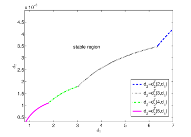
a) b)

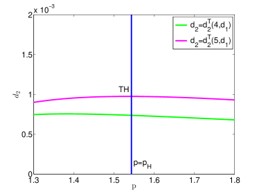
Figure 15: a) Partial Turing bifurcation curve $l^{T}$ of system (11) with the parameters $a=0.23,r=1.1,m=0.31,l=2,c=0.25<\frac{1}{r(1-a)},p=1.4<p_{H}$. b) When $a=0.23,r=1.1,m=0.31,l=2,c=0.25,d_{1}=1.496$, Turing bifurcation curve $d_{2}=d_{2}(5,d_{1})$ intersects line $p=p_{H}$ at $TH~{}(1.5432,0.0009)$, which is a Turing-Hopf bifurcation point.

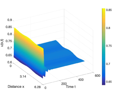
a) b)

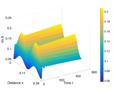
Figure 16: a) The Prey pattern and b) the predator pattern for system (11) with the parameters $a=0.23,r=1.1,m=0.31,l=2,,c=0.25,p=1.4,d_{1}=1.496,d_{2}=0.000688$. The patterns indicate instability induced by diffusion for the prey and predator. Initial conditions are $u(x,0)=0.6+0.1\cos 2x$, $v(x,0)=0.08-0.02\cos 2x$.

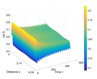
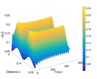
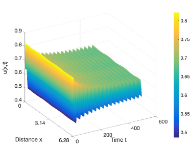
a) b) c) d)

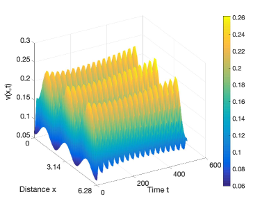
Figure 17: Two spatially inhomogeneous periodic solutions coexist when we choose $a=0.23,m=0.31,r=1.1$, $l=2$, $c=0.25$, $p=p_{H}=1.5432$, $d_{1}=1.496$, and $d_{2}=0.00081$ in system (11). Initial conditions are $u(x,0)=0.6+0.1\cos 2x$, $v(x,0)=0.08-0.02\cos 2x$ for a) b), and $u(x,0)=0.6+0.1\cos 3x$, $v(x,0)=0.08-0.02\cos 3x$ for c) d).

To illustrate the dynamics of (11) in the case of strong cooperation, we choose $c=8$ such that $c>\frac{1}{r(1-a)}$. Let $p=0.8<p_{H}=0.8306$. From (16) and (17), we can draw partial Turing bifurcation curve $l^{T}$ on $d_{1}-d_{2}$ plane (see Fig. 18 a)). The constant steady state $E^{*}(0.7392,0.0864)$ is stable when we choose $d_{1}$ and $d_{2}$ in the region above $l^{T}$.

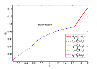
a) b)

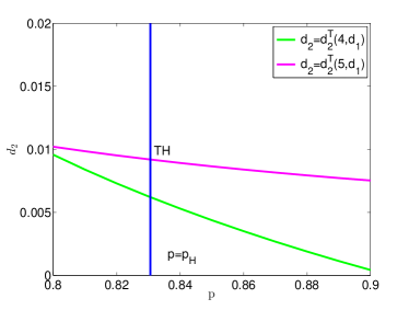
Figure 18: a) Partial Turing bifurcation curve $l^{T}$ of system (11) with the parameters $a=0.23,r=1.1,m=0.31,l=2,c=8,p=0.8<p_{H}$. b) b) When $a=0.23,r=1.1,m=0.31,l=2,c=8,d_{1}=0.13$, Turing bifurcation curve $d_{2}=d_{2}(5,d_{1})$ intersects line $p=p_{H}$ at $TH~{}(0.8306,0.009)$, which is a Turing-Hopf bifurcation point.

If we choose $d_{1}=0.13$ and $d_{2}=0.006$ in the region below $l^{T}$, from Theorem 10, the steady state $E^{*}$ of the diffusive system is Turing unstable. There are three spatially inhomogeneous steady states coexist when we choose three different initial values.

If we fix $d_{1}=0.13$, from (16), we can draw Turing bifurcation curve on $p-d_{2}$ plane (see Fig. 18 b)), and $d_{2}=d_{2}^{T}(5,d_{1})$ intersects line $p=p_{H}$ at $TH~{}(0.8306,0.009)$. Choosing $p=0.8306,d_{2}=0.0065$ near $TH$, we can illustrate two stable spatially inhomogeneous periodic solutions coexisting when we choose two different initial values (see Fig. 19).

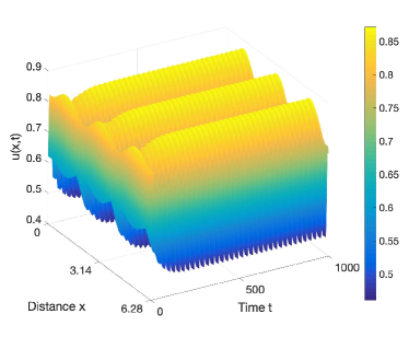
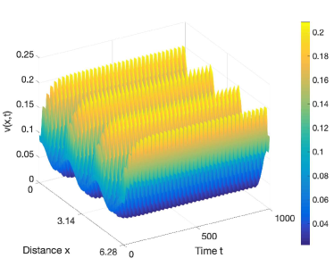
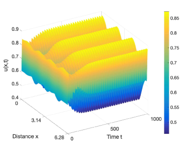
a) b) c) d)

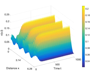
Figure 19: Two stable spatially inhomogeneous periodic solutions of system (11) coexist with $a=0.23,m=0.31,r=1.1$, $l=2$, $c=8$, $p=p_{H}=0.8306$, $d_{1}=0.13$, and $d_{2}=0.0065$. Initial values are $u(x,0)=0.6+0.1\cos 4x$, $v(x,0)=0.08-0.02\cos 4x$ for a) b), and $u(x,0)=0.6+0.1\cos 3x$, $v(x,0)=0.08-0.02\cos 3x$ for c) d).

4 The dynamics of diffusive system with two delays

It has been widely accepted that time delays have very complex effect on the dynamics of a system, for example, some delays can destroy the stability of equilibria and induce various oscillations and periodic solutions. There are time delays in almost every process of population interaction, so it is more realistic to introduce time delays when we model the interaction of predator and prey. For example, after the predator consuming the prey, the reproduction of predator is not instantaneous but taking time for the transition from prey biomass into predator biomass. We call this kind of time delay as a gestation delay. There is an extensive literature about the studies of the dynamics of predator-prey models with the effect of time delay due to gestation of the predator (see, for example, Kuang Ygestation ; Gopalsamy Kgestation ; Martin Agestation ; Xia Jgestation and references cited therein). Mature delay of the prey has also been considered Wright E ; RM May ; XuCdelay ; Yandelay . However, to the best of our knowledge, there is very little literatures on delayed predator-prey system with Allee effect JankovicAl]eedelay .

We consider the following diffusive system with two delays

$$\left\{\begin{array}[]{l}\dfrac{\partial u(x,t)}{\partial t}=d_{1}\Delta u(x,t)+ru(x,t)[1-u(x,t-\tau_{1})](u(x,t)-a)\\ ~{}~{}~{}~{}~{}~{}~{}~{}~{}~{}~{}~{}~{}~{}~{}~{}-(1+cv(x,t))u(x,t)v(x,t),~{}~{}~{}~{}~{}~{}~{}~{}~{}~{}~{}~{}~{}~{}~{}~{}~{}~{}~{}~{}~{}~{}~{}~{}~{}~{}~{}~{}~{}~{}~{}~{}~{}~{}~{}~{}~{}~{}~{}~{}~{}~{}~{}~{}~{}~{}~{}~{}~{}x\in(0,l\pi),\\ \dfrac{\partial v(x,t)}{\partial t}=d_{2}\Delta v(x,t)+mv(x,t)\left[pu(x,t-\tau_{2})\left(1+cv(x,t-\tau_{2})\right)-1\right],~{}x\in(0,l\pi),{}\\ \partial_{v}u(x,t)=0,~{}~{}\partial_{v}v(x,t)=0,~{}~{}~{}~{}~{}~{}~{}~{}~{}~{}~{}~{}~{}~{}~{}~{}~{}~{}~{}~{}~{}~{}~{}~{}~{}~{}~{}~{}~{}~{}~{}~{}~{}~{}~{}~{}~{}~{}~{}~{}~{}~{}~{}~{}~{}~{}~{}~{}~{}~{}~{}~{}~{}~{}~{}~{}~{}~{}~{}~{}~{}~{}~{}~{}x=0,l\pi.\\ \end{array}\right.$$ (19)

Here $\tau_{1}$ is the time delay due to the maturation of the prey, $\tau_{2}$ is time delay due to gestation of the predator, and we define $\tau={\rm max}\{\tau_{1},\tau_{2}\}$.

Systems with multiple delays have attracted much attention K.L. Cooke ; H. I. Freedman ; J. Wei and S. Ruan ; Xu J ; twodelays ; Huang C . Generally, delay may induce Hopf bifurcation, and if Hopf bifurcation curves intersect, double Hopf bifurcation may arise. To figure out the effect of delay on the dynamics of systems, Hopf bifurcation and double Hopf bifurcation induced by delay have been investigated Yudouble ; Dujia1 ; Ma double ; Campell double . However, in most of literatures we mentioned above, the system is reduced into a system with one delay. In fact, systems with multiple delays conform to reality better than one single delay. Recently, the research on the dynamics and bifurcation analysis of system with two simultaneously varying delays are of great interest to scholars. In twodelays ; Ge Jtwodelay , the double Hopf bifurcation induced by two delays are studied by different methods. Through the analysis of double Hopf bifurcation, we can classify the topological structures of various bifurcating solutions. By the classification, the dynamics in the neighbourhood of the double Hopf bifurcation point in system can be obtained completely.

In the previous section, we have found the conditions of stability and Turing instability of constant steady state $E^{*}$ of system (19) when $\tau_{1}=\tau_{2}=0$. We know that if $p<p_{H}$ and $d_{2}>d_{2}^{T}(n,d_{1})$ for all $n\in\mathbb{N}$, the steady state $E^{*}$ is locally asymptotically stable. In this section, we investigate the diffusive system (19) under the assumption $p<p_{H}$ and $d_{2}>d_{2}^{T}(n,d_{1})$, and focus on the effect of two delays on the dynamics of the diffusive system near $E^{*}$.

4.1 Hopf and double Hopf bifurcation induced by two delays

In this subsection, we investigate the existence of Hopf bifurcation induced by two delays by the method of stability switching curves given in Ref. Lin X , and give the condition of the existence of double Hopf bifurcation.

The linearization of system (19) at the steady state $E^{*}(u^{*},v^{*})$ is given by

$$\frac{\partial}{\partial t}\left(\begin{array}[]{l}u(x,t)\\ v(x,t)\\ \end{array}\right)=(D\Delta+A)\left(\begin{array}[]{l}u(x,t)\\ v(x,t)\\ \end{array}\right)+B\left(\begin{array}[]{l}u(x,t-\tau_{1})\\ v(x,t-\tau_{1})\\ \end{array}\right)+C\left(\begin{array}[]{l}u(x,t-\tau_{2})\\ v(x,t-\tau_{2})\\ \end{array}\right),$$ (20)

where

$$\begin{array}[]{l}A=\left(\begin{array}[]{cc}ru^{*}(1-u^{*})&-2cu^{*}v^{*}-u^{*}\\ 0&0\\ \end{array}\right),~{}B=\left(\begin{array}[]{cc}-ru^{*}(u^{*}-a)&0\\ 0&0\\ \end{array}\right),\\ C=\left(\begin{array}[]{cc}0&0\\ mp(1+cv^{*})v^{*}&mpcu^{*}v^{*}\\ \end{array}\right),D={\rm diag}(d_{1},d_{2}).\end{array}$$ (21)

$u(x,t)$ and $v(x,t)$ satisfy the homogeneous Neumann boundary condition.

From Wu JWu , the corresponding characteristic equation of Eq. (20) is

$${\rm det}\left(\lambda I-M_{n}-A-Be^{-\lambda\tau_{1}}-Ce^{-\lambda\tau_{2}}\right)=0,$$ (22)

where $I$ is a $2\times 2$ identity matix, $M_{n}=-n^{2}/l^{2}{\rm diag}(d_{1},d_{2})$, $n\in\mathbb{N}_{0}=\{0,1,2,...\}$. Eq. (22) can be written in the following form:

$$D_{n}(\lambda;\tau_{1},\tau_{2})=P_{0,n}(\lambda)+P_{1,n}(\lambda)e^{-\lambda\tau_{1}}+P_{2,n}(\lambda)e^{-\lambda\tau_{2}}+P_{3,n}(\lambda)e^{-\lambda(\tau_{1}+\tau_{2})}=0,$$ (23)

where

$$\begin{array}[]{l}P_{0,n}(\lambda)=(\lambda+d_{1}\frac{n^{2}}{l^{2}}-a_{11})(\lambda+d_{2}\frac{n^{2}}{l^{2}}),\\ P_{1,n}(\lambda)=-b_{11}(\lambda+d_{2}\frac{n^{2}}{l^{2}}),\\ P_{2,n}(\lambda)=-c_{22}(\lambda+d_{1}\frac{n^{2}}{l^{2}}-a_{11})-a_{12}c_{21},\\ P_{3,n}(\lambda)=b_{11}c_{22}.\end{array}$$ (24)

The characteristic equation with the form of Eq. (23) has been investigated by Lin and Wang Lin X . They derived an explicit expression for the stability switching curves, on which there is a pair of purely imaginary roots for Eq. (23). Moreover, they gave a criterion to determine the crossing directions, i.e., on which side of the stability switching curve there are two more characteristic roots with positive real parts. Using this method, we can find all the stability switching curves in the $(\tau_{1},\tau_{2})$ plane, and determine the crossing directions. We leave the details in the A and B.

Moreover, we have the following Hopf bifurcation theorem with two parameters.

      Theorem 11.

For each $j\in\{1,2,\cdots,N\}$, $\mathcal{T}_{n}^{j}$, defined by (40), is a Hopf bifurcation curve in the following sense: for any $p\in\mathcal{T}_{n}^{j}$ and for any smooth curve $\Gamma$ intersecting with $\mathcal{T}_{n}^{j}$ transversely at $p$, we define the tangent of $\Gamma$ at $p$ by $\overrightarrow{l}$. If $\frac{\partial{\rm Re}\lambda}{\partial\overrightarrow{l}}\mid_{p}\neq 0$, and the other eigenvalues of (23) at $p$ have non-zero real parts, then system (19) undergoes a Hopf bifurcation at $p$ when parameters $(\tau_{1},\tau_{2})$ cross $\mathcal{T}_{n}^{j}$ at $p$ along $\Gamma$.

The theorem can be proved by a similar method in twodelays .

      Remark 7.

Suppose that $\mathcal{T}_{k_{1}}^{j_{1}}$ and $\mathcal{T}_{k_{2}}^{j_{2}}$ intersect at a point $(\tau_{1},\tau_{2})$, with the corresponding values of $\omega$ being $\omega_{j_{1},k_{1}}\in\Omega_{j_{1},k_{1}}$ and $\omega_{j_{2},k_{2}}\in\Omega_{j_{2},k_{2}}$. Then there are two pairs of purely imaginary roots of (23) at the intersection, which are $\pm i\omega_{j_{1},k_{1}}$ and $\pm i\omega_{j_{2},k_{2}}$, denoted by $\pm i\omega_{1}$ and $\pm i\omega_{2}$ for convenience. Thus, system (19) may undergo double Hopf bifurcations at the intersection of two stability switching curves near the constant steady state $E^{*}$.

4.2 Normal form on the center manifold for double Hopf bifurcation

In this subsection, applying the normal form method of partial functional differential equations Faria , we derive normal form of double Hopf bifurcation taking two delays as bifurcation parameters. Then, we can classify the topological structures of various bifurcating solutions, and get the dynamics in the neighbourhood of the double Hopf bifurcation point in system (19).

For the Neumann boundary condition, we define the real-valued Sobolev space

$$X=\{(u,v)^{T}\in H^{2}(0,l\pi)\times H^{2}(0,l\pi)\arrowvert\dfrac{\partial u}{\partial x}=\dfrac{\partial v}{\partial x}=0,x=0,l\pi\},$$

and the abstract space $\mathcal{C}=C([-1,0],X)$. Define the complexification space of the real-valued Hilbert space $X$ by

$$X_{\mathbb{C}}:=X\oplus iX=\{U_{1}+iU_{2}:U_{1},U_{2}\in X\},$$

with the general complex-value $L^{2}$ inner product

$$\langle U,V\rangle=\int_{0}^{l\pi}(\overline{u}_{1}v_{1}+\overline{u}_{2}v_{2})dx,~{}~{}\mbox{for}~{}~{}U=(u_{1},u_{2})^{T},V=(v_{1},v_{2})^{T}\in X_{\mathbb{C}}.$$

Let $\mathscr{C}:=C([-1,0],X_{\mathbb{C}})$ denotes the phase space with the sup norm, and write $u^{t}\in\mathscr{C}$ for $u^{t}(\theta)=u(t+\theta)$, $-1\leq\theta\leq 0$.

Without loss of generality, we assume $\tau_{1}<\tau_{2}$ in this section. Denote the double Hopf bifurcation point by $(\tau_{1}^{*},\tau_{2}^{*})$. Let $\overline{u}(x,t)=u(x,\tau_{2}t)-u^{*},\overline{v}(x,t)=v(x,\tau_{2}t)-v^{*}$, and set $\sigma_{1}=\tau_{1}-\tau_{1}^{*}$ and $\sigma_{2}=\tau_{2}-\tau_{2}^{*}$ as two bifurcation parameters. Drop the bars, and denote $U(t)=(u(t),v(t))^{T}$, then system (19) can be written as

$$\dfrac{dU(t)}{dt}=D(\tau_{1}^{*}+\sigma_{1},\tau_{2}^{*}+\sigma_{2})\Delta U(t)+L(\tau_{1}^{*}+\sigma_{1},\tau_{2}^{*}+\sigma_{2})(U^{t})+F(\tau_{1}^{*}+\sigma_{1},\tau_{2}^{*}+\sigma_{2},U^{t}),$$ (25)

where

$$\begin{array}[]{l}D(\tau_{1}^{*}+\sigma_{1},\tau_{2}^{*}+\sigma_{2})=(\tau_{2}^{*}+\sigma_{2})D=\tau_{2}^{*}D+\sigma_{2}D,\\ L(\tau_{1}^{*}+\sigma_{1},\tau_{2}^{*}+\sigma_{2})(\phi)=(\tau_{2}^{*}+\sigma_{2})\left[A\phi(0)+B\phi(-\frac{\tau_{1}^{*}+\sigma_{1}}{\tau_{2}^{*}+\sigma_{2}})+C\phi(-1))\right],\\ F(\tau_{1}^{*}+\sigma_{1},\tau_{2}^{*}+\sigma_{2},\phi)=(\tau_{2}^{*}+\sigma_{2})(F_{1},F_{2})^{T},\end{array}$$

with $A,~{}B$, $C$ and $D$ being defined in (21), and for $\varphi\in\mathcal{C}$

$$\begin{array}[]{l}F_{1}=r(1-u^{*})\phi_{1}^{2}(0)-(1+2cv^{*})\phi_{1}(0)\phi_{2}(0)+(ra-2ru^{*})\phi_{1}(0)\phi_{1}(-\frac{\tau_{1}^{*}+\sigma_{1}}{\tau_{2}^{*}+\sigma_{2}})\\ ~{}~{}~{}~{}~{}~{}~{}~{}~{}~{}-cu^{*}\phi_{2}^{2}(0)-r\phi_{1}^{2}(0)\phi_{1}(-\frac{\tau_{1}^{*}+\sigma_{1}}{\tau_{2}^{*}+\sigma_{2}})-c\phi_{1}(0)\phi_{2}^{2}(0),\end{array}$$

and

$$\begin{array}[]{l}F_{2}=mp(1+cv^{*})\phi_{2}(0)\phi_{1}(-1)+mpc[u^{*}\phi_{2}(0)+v^{*}\phi_{1}(-1)+\phi_{2}(0)\phi_{1}(-1)]\phi_{2}(-1).\end{array}$$

Consider the linearized system of (25)

$$\dfrac{dU(t)}{dt}=\tau_{2}^{*}D\Delta U(t)+\tau_{2}^{*}(AU^{t}(0)+BU^{t}(-\tau_{1}^{*}/\tau_{2}^{*})+CU^{t}(-1))\stackrel{{\scriptstyle\vartriangle}}{{=}}D_{0}\Delta U(t)+L_{0}(U^{t}).$$ (26)

We know that the normalized eigenfunctions of $D\Delta$ on $X$ corresponding to the eigenvalues $-d_{1}\frac{n^{2}}{l^{2}}$ and $-d_{2}\frac{n^{2}}{l^{2}}$( $n\in\mathbb{N}_{0}=\{0,1,2,\cdots\}$) are

$$\beta_{n}^{1}(x)=\gamma_{n}(x)(1,0)^{T}~{}\mbox{and}~{}~{}\beta_{n}^{2}(x)=\gamma_{n}(x)(0,1)^{T},$$

respectively, where $\gamma_{n}(x)=\dfrac{\cos\frac{n}{l}x}{\parallel\cos\frac{n}{l}x\parallel_{L^{2}}}$. Define $\mathscr{B}_{n}:={\rm span}\left\{\langle v(\cdot),\beta_{n}^{j}\rangle\beta_{n}^{j}~{}\arrowvert~{}v\in\mathscr{C},j=1,2\right\}$, satisfying $L(\mathscr{B}_{n})(\tau_{1},\tau_{2})\subset{\rm span}\{\beta_{n}^{1},\beta_{n}^{2}\}$. Denote $\left\langle v(\cdot),\beta_{n}\right\rangle=\left(\langle v(\cdot),\beta_{n}^{1}\rangle,\langle v(\cdot),\beta_{n}^{2}\rangle\right)^{T}.$

Write system (25) as

$$\dfrac{dU(t)}{dt}=D_{0}\Delta U(t)+L_{0}(U^{t})+\widetilde{F}(\sigma,U^{t}),$$ (27)

where

$$\widetilde{F}(\sigma,U^{t}) =\sigma_{2}(D\Delta U^{t}(0)+AU^{t}(0)+BU^{t}(-\tau_{1}^{*}/\tau_{2}^{*})+CU^{t}(-1))$$

$$+(\tau_{2}^{*}+\sigma_{2})B(U^{t}(-(\tau_{1}^{*}+\sigma_{1})/(\tau_{2}^{*}+\sigma_{2}))-U^{t}(-\tau_{1}^{*}/\tau_{2}^{*}))+F(\tau_{1}^{*}+\sigma_{1},\tau_{2}^{*}+\sigma_{2},U^{t}).$$

System (27) can be rewritten as an abstract ordinary differential equation on $\mathscr{C}$ Faria

$$\frac{d}{dt}U^{t}=\mathcal{A}U^{t}+X_{0}\widetilde{F}(\sigma,U^{t}),$$ (28)

where $\mathcal{A}$ is the infinitesimal generator of the $C_{0}$-semigroup of solution maps of the linear equation (25), defined by

$$\mathcal{A}\varphi=\dot{\varphi}+X_{0}[D_{0}\Delta\varphi(0)+L_{0}(\varphi)-\dot{\varphi}(0)],$$ (29)

with ${\rm dom}(\mathcal{A})=\{\varphi\in\mathscr{C}:\dot{\varphi}\in\mathscr{C},\varphi(0)\in{\rm dom}(\Delta)\}$, and $X_{0}$ is given by $X_{0}(\theta)=0$ for $\theta\in[-1,0)$ and $X_{0}(0)=I$. Clearly, $\mathcal{A}:\mathscr{C}_{0}^{1}\cap\mathscr{C}\rightarrow\mathscr{C}.$

Then on $\mathscr{B}_{n}$, the linear equation

$$\frac{d}{dt}U(t)=D_{0}\Delta U(t)+L_{0}(U^{t})$$

is equivalent to the retarded functional differential equation on $\mathbb{C}^{2}$:

$$\dot{z}(t)=-\frac{n^{2}}{l^{2}}D_{0}z(t)+L_{0}z^{t}.$$ (30)

By the Riesz representation theorem, there exists a matrix whose components are bounded variation functions $\eta_{k}\in BV([-1,0],\mathbb{R}^{2\times 2})$ such that

$$-\frac{n_{k}^{2}}{l^{2}}D_{0}\varphi(0)+L_{0}(\varphi)=\int_{-1}^{0}d\eta_{k}(\theta)\varphi(\theta),\varphi\in\mathscr{C}.$$

Let $A_{k}$ ($k=1,2$) denote the infinitesimal generator of the semigroup generated by (30), and $A_{k}^{*}$ denote the formal adjoint of $A_{k}$ under the bilinear form

$$(\alpha,\beta)_{k}=\alpha(0)\beta(0)-\int_{-1}^{0}\int_{0}^{\theta}\alpha(\xi-\theta)d\eta_{k}(\theta)\beta(\xi)d\xi.$$

The calculations of normal form are very long, so we leave them in supplementary materials. Based on the derivation in supplementary materials, the normal form truncated to the third order on the center manifold for double Hopf bifurcation is obtained. Making the polar coordinate transformation, then we obtain the following system corresponding to the truncated normal form

$$\dot{\rho}_{1}=r_{1}(\nu_{1}+r_{1}^{2}+br_{2}^{2}),$$ (31)

$$\dot{\rho}_{2}=r_{2}(\nu_{2}+cr_{1}^{2}+dr_{2}^{2}),$$

where

$$\nu_{1}=\epsilon_{1}({\rm Re}B_{11}\sigma_{1}+{\rm Re}B_{21}\sigma_{2}),\nu_{2}=\epsilon_{1}({\rm Re}B_{13}\sigma_{1}+{\rm Re}B_{23}\sigma_{2}),b=\frac{\epsilon_{1}\epsilon_{2}{\rm Re}B_{1011}}{{\rm Re}B_{0021}},c=\frac{{\rm Re}B_{1110}}{{\rm Re}B_{2100}},d=\epsilon_{1}\epsilon_{2},$$

and $B_{11},B_{21},B_{13},B_{23},B_{1011},B_{0021},B_{1110}$ and $B_{2100}$ are the coefficients of the normal form obtained in supplementary materials. From chapter 7.5 in Ref. Guckenheimer , there are twelve distinct kinds of unfoldings for Eq. (31).

4.3 Numerical simulations for diffusive system with two delays

In this section, we carry out some numerical simulations for diffusive system (19). Fix

$$a=0.23,r=1.1,m=0.31,l=2,$$

which is the same as in (18). Fix $c=0.25$ such that $c<\frac{1}{r(1-a)}$, and choose $p=1.2<p_{H}$, $d_{1}=0.3$ and $d_{2}=0.4$, such that $d_{2}>d_{2}^{T}(1,d_{1})$ for all $n\in\mathbb{N}$ . From Theorem 10, one can get the unique constant steady state $E^{*}(0.80945,0.11797)$ is locally asymptotically stable.

Now we illustrate the effect of two delays on the dynamics (19). Following the steps in A and B, we can draw all the stability curves on $(\tau_{1},\tau_{2})$ plane, and decide the crossing direction, which are shown in Fig. 22-26 in C. Combining all the stability switching curves together, and zooming in the part of $(\tau_{1},\tau_{2})\in[0,5]\times[0,20]$, we get the Hopf bifurcation curves shown in Fig. 20 a). Consider the bottom left region bounded by left-most curve of $\mathcal{T}^{1}_{0}$ and the lowest curve of $\mathcal{T}^{2}_{0}$ (see Fig. 20 a)), which are both part of $\mathcal{T}_{0}$. Since the crossing directions of the two switching curves (the black line and blue line) are all pointing outside of the region, the constant steady state $E^{*}$ is stable in the bottom left region. Moreover, the two stability switching curves intersect at the point $(2.21407,15.0019)$, which is the double Hopf bifurcation point, denoted by HH. For HH, $\omega_{1}=0.1078$, $\omega_{2}=0.4920$. Using the normal form derivation process given in supplementary materials, we have $B_{11}=-0.0512$, $B_{21}=0.0478$, $B_{13}=1.7736$, $B_{23}=-0.0706$, $B_{2100}=-0.7294$, $B_{1011}=-1.5826$, $B_{0021}=-0.2410$, $B_{1110}=-10.8681$. Furthermore, we have the normal form (31) with $\epsilon_{1}=-1,\epsilon_{2}=-1,b=6.5658,c=14.8998,d=1$, and $d-bc=-96.8306$. According to chapter 7.5 in Ref. Guckenheimer , case Ib arises, and we have the bifurcation set near HH showing in Fig. 20 b). In region $D_{1}$, the positive equilibrium is asymptotically stable. In region $D_{2}$ or $D_{6}$, there is a stable periodic solution. When the parameters cross into the region D4, there are two stable momogeneous periodic solutions coexisting in D4.

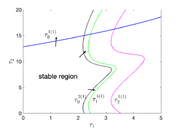
a) b)

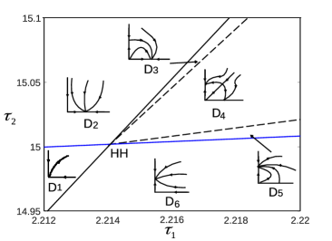
Figure 20: a) The left-most curve and the lowest curve of $\mathcal{T}_{0}$ intersect at $(\tau_{1},\tau_{2})=(2.2140,15.0019)$, which is a double Hopf bifurcation point on the $\tau_{1}-\tau_{2}$ plane. Crossing directions are marked by arrows. b) The complete bifurcation sets near double Hopf bifurcation point HH.

5 Concluding remarks

The first part of this paper is mainly about the dynamics of the ODE predator-prey model (3) with Allee effect in prey and cooperative hunting in predator. We start with the ODE system in the case of weak cooperation. Taking $p$, the convertion rate, as the bifurcation parameter, we prove that there is a loop of heteroclinic orbits between $E_{1}$ and $E_{a}$ formed by the intersection of the stable manifold of $E_{a}$ and the unstable manifold of $E_{1}$ when $p=p^{\#}$ ($p^{\#}>1$). It shows that $p^{\#}$ is an important threshold, which distinguishes the globally stability for $E_{0}$ and the existence of a separatrix curve. To be specific, when $p>p^{\#}$, $E_{0}$ is globally stable, which means the extinction of both species, and we call the phenomenon overexploitation. When $p<p^{\#}$, there is a separatrix curve $\Gamma_{p}^{s}$, which is determined by the stable manifold of $E_{a}$. High initial predator density will lead to extinction for both species, and conversely low initial predator density will approach either a steady state or a periodic oscillation. When $p<1$, $E_{1}(1,0)$ is locally stable, which means that the prey achieves its carrying capacity and the predator is extinct. When $1<p<p_{H}$, the stable state becomes $E^{*}$, which implies the coexistence of both species. When $p$ crosses $p_{H}$, the stable state switches into a limit cycle. The period of the limit cycle increases with $p$, and tends to $\infty$ as $p\rightarrow p^{\#}$. The existence of a limit cycle with a large amplitude increases the risk of the extinction for the predator.

In the case of strong cooperation, three different cases are considered. We prove the existence of a loop of heteroclinic orbits between $E_{1}$ and $E_{a}$ when $p=p^{\#}$ in the first and second cases and nonexistence of such a loop of heteroclinic orbits in the third case. We also exhibit the existence of loop of heteroclinic orbits among $E_{R}^{*}$, $E_{a}$ and $E_{1}$ formed by the unstable manifold of $E_{R}^{*}$ and the unstable manifold $E_{a}$ when $p=\overline{p}^{\#}$, and a homoclinic cycle when $p=p_{hom}$ by numerical simulations in case 3. When $p>p^{\#}$ in case 1 and case 2 ($p>\overline{p}^{\#}$ in case 3), both species distinct. When $1<p<p^{\#}$ in case 1 and case 2, there is a separatrix curve $\Gamma_{p}^{s}(E_{a})$, and there are two stable states coexisting, which are extinction for both species and coexistence or oscillation. When $p<p^{\#}$ (or $p<\overline{p}^{\#}$) and $p_{SN}<p<1$, there are two separatrix curves, the stable manifold of $E_{a}$ and the stable manifold of $E_{R}^{*}$, separating the first quadrant into three parts. If the initial population is above the stable manifold of $E_{a}$, both species are extinct; if the initial population is inside the stable manifold of $E_{R}^{*}$, the stable state can be $E^{*}$ or limit cycle; if the initial population is below the stable manifold of $E_{a}$ and outside the stable manifold of the stable manifold of $E_{R}^{*}$, the prey achieves its carrying capacity and the predator is extinct. When $p<p_{SN}$, there is one separatrix curve $\Gamma_{p}^{s}(E_{a})$, and there are two stable states coexisting. The species with initial population above the separatrix finally become extinct, however only the prey survive when initial population is below it.

There is a unique equilibrium for weak cooperation when $1<p<\frac{1}{a}$. It is shown that there are at most two stable states coexist for different initial values separated by the stable manifold of $E_{a}$. There are two interior equilibria $E^{*}$ and $E_{R}^{*}$ in the case of strong cooperation when $p_{SN}<p<1$. The equilibrium $E_{R}^{*}$ brings one more separatrix curve than the case of weak cooperation, thus there may be three stable states coexisting.

In the second part, we consider the corresponding diffusive system, and focus on the effect of diffusion on the dynamics. Taking diffusion coefficients $d_{1}$ and $d_{2}$ as bifurcation parameters, we give the conditions of existence of Turing instability and Turing-Hopf bifurcation. We illustrate complex dynamics of the diffusive system, including the existence of spatially inhomogeneous steady state, coexistence of two spatially inhomogeneous periodic solutions.

The third part of this paper is about the diffusive system with two delays. We discuss the joint effect of two delays on the dynamical behavior of the diffusive system. Applying the method of stability switching curves, we find all the stability switching curves at which the characteristic roots are purely imaginary. Combining the geometrical and analytic method, we can decide the crossing direction of the characteristic roots as long as we confirm the positive direction for stability switching curves. Then we can get the condition of existence of Hopf bifurcation. By searching the intersection of stability switching curves near the stable region, we get the double Hopf bifurcation point. Through the calculation of normal form of the system, we get the corresponding unfolding system and the bifurcation set, from which we can figure out the complete dynamics near the bifurcation point on the $(\tau_{1},\tau_{2})$ parametric plane. We theoretically prove and illustrate that near the bifurcation point, there are the phenomena of the stability of positive equilibrium, stable periodic solutions and coexistence of two periodic solutions.

Appendix A Stability switching curves

Applying the method proposed in Lin and Wang Lin X to find the stability switching curves, we need to verify the assumptions (i)-(iv) in Ref. Lin X .

• Finite number of characteristic roots on $\mathbb{C}_{+}=\{\lambda\in\mathbb{C}:{\rm Re}\lambda>0\}$ under the condition

  $${\rm deg}(P_{0,n}(\lambda))\geq{\rm max}\{{\rm deg}(P_{1,n}(\lambda)),{\rm deg}(P_{2,n}(\lambda)),{\rm deg}(P_{3,n}(\lambda))\}.$$

• $P_{0,n}(0)+P_{1,n}(0)+P_{2,n}(0)+P_{3,n}(0)\neq 0$.

• $P_{0,n}(\lambda),P_{1,n}(\lambda),P_{2,n}(\lambda),P_{3,n}(\lambda)$ are coprime polynomials.

• $\lim\limits_{\lambda\rightarrow\infty}\left(\left|\frac{P_{1,n}(\lambda)}{P_{0,n}(\lambda)}\right|+\left|\frac{P_{2,n}(\lambda)}{P_{0,n}(\lambda)}\right|+\left|\frac{P_{3,n}(\lambda)}{P_{0,n}(\lambda)}\right|\right)<1$.

In fact, condition (i) follows from Ref. J. Hale . In fact $P_{0,n}(0)+P_{1,n}(0)+P_{2,n}(0)+P_{3,n}(0)=J_{n}$, which is determined in (15). Since we assume $p<p_{H}$ and $d_{2}>d_{2}^{T}(n,d_{1})$ for all $n\in\mathbb{N}$, from Theorem 10, the constant steady state $E^{*}$ is locally asymptotically stable, and $J_{n}>0$ for all $n\in\mathbb{N}$. Thus, condition (ii) satisfies. From the expressions of $P_{0,n}(\lambda),P_{1,n}(\lambda),P_{2,n}(\lambda),P_{3,n}(\lambda)$ in (24), condition (iii) is obviously satisfied. From (24), we know

$$\lim\limits_{\lambda\rightarrow\infty}\left(\left|\frac{P_{1,n}(\lambda)}{P_{0,n}(\lambda)}\right|\right)=\lim\limits_{\lambda\rightarrow\infty}\left(\left|\frac{P_{2,n}(\lambda)}{P_{0,n}(\lambda)}\right|\right)=\lim\limits_{\lambda\rightarrow\infty}\left(\left|\frac{P_{3,n}(\lambda)}{P_{0,n}(\lambda)}\right|\right)=0,$$

which means that (iv) are satisfied.

From K.L. Cooke ; Ruan wei , we have the following lemma.

      Lemma 3.

As the delays $(\tau_{1},\tau_{2})$ vary continuously in $\mathbb{R}_{+}^{2}$, the number of zeros (counting multiplicity) of $D_{n}(\lambda;\tau_{1},\tau_{2})$ on $\mathbb{C}_{+}$ can change only if a zero appears on or cross the imaginary axis.

From condition (ii), $\lambda=0$ is not a root of (23). Now we are in the position of seeking all the points $(\tau_{1},\tau_{2})$ such that $D_{n}(\lambda;\tau_{1},\tau_{2})=0$ has at least one root on the imaginary axis, on which the stability of equilibrium $E^{*}$ may switch. Substituting $\lambda=i\omega~{}(\omega>0)$ into (23),

$$(P_{0,n}(i\omega)+P_{1,n}(i\omega)e^{-i\omega\tau_{1}})+(P_{2,n}(i\omega)+P_{3,n}(i\omega)e^{-i\omega\tau_{1}})e^{-i\omega\tau_{2}}=0.$$

Due to $|e^{-i\omega\tau_{2}}|=1$, we get that

$$|P_{0,n}(i\omega)+P_{1,n}(i\omega)e^{-i\omega\tau_{1}}|=|P_{2,n}(i\omega)+P_{3,n}(i\omega)e^{-i\omega\tau_{1}}|,$$

Thus, we have the following equality

$$|P_{0,n}(i\omega)|^{2}+|P_{1,n}(i\omega)|^{2}-|P_{2,n}(i\omega)|^{2}-|P_{3,n}(i\omega)|^{2}=2A_{1,n}(\omega)\cos(\omega\tau_{1})-2B_{1,n}(\omega)\sin(\omega\tau_{1}),$$ (32)

where

$$A_{1,n}(\omega)={\rm Re}(P_{2,n}(i\omega)\overline{P}_{3,n}(i\omega)-P_{0,n}(i\omega)\overline{P}_{1,n}(i\omega))=\sqrt{A_{1,n}(\omega)^{2}+B_{1,n}(\omega)^{2}}\cos(\varphi_{1,n}(\omega)),$$

$$B_{1,n}(\omega)={\rm Im}(P_{2,n}(i\omega)\overline{P}_{3,n}(i\omega)-P_{0,n}(i\omega)\overline{P}_{1,n}(i\omega))=\sqrt{A_{1,n}(\omega)^{2}+B_{1,n}(\omega)^{2}}\sin(\varphi_{1,n}(\omega)),$$

if $A_{1,n}(\omega)^{2}+B_{1,n}(\omega)^{2}>0$, with $\varphi_{1,n}(\omega)=\angle\{P_{2,n}(i\omega)\overline{P}_{3,n}(i\omega)-P_{0,n}(i\omega)\overline{P}_{1,n}(i\omega)\}\in(-\pi,\pi]$. Thus, we can write Eq. (32) as

$$|P_{0,n}(i\omega)|^{2}+|P_{1,n}(i\omega)|^{2}-|P_{2,n}(i\omega)|^{2}-|P_{3,n}(i\omega)|^{2}=2\sqrt{A_{1,n}(\omega)^{2}+B_{1,n}(\omega)^{2}}\cos(\varphi_{1,n}(\omega)+\omega\tau_{1}).$$ (33)

Denote

$$\Sigma^{1}_{n}=\left\{\omega\in\mathbb{R}_{+}:\left((P_{0,n}(i\omega)|^{2}+|P_{1,n}(i\omega)|^{2}-|P_{2,n}(i\omega)|^{2}-|P_{3,n}(i\omega)|^{2}\right)^{2}\leq 4(A_{1,n}(\omega)^{2}+B_{1,n}(\omega)^{2})\right\}.$$ (34)

We can easily know that there is $\tau_{1}\in\mathbb{R}_{+}$ satisfying Eq. (33) if and only if $\omega\in\Sigma^{1}_{n}$. In fact, (34) also includes the case $A_{1,n}^{2}(\omega)+B_{1,n}^{2}(\omega)=0$.

Define

$$\theta_{1,n}(\omega)=\arccos\left(\dfrac{|P_{0,n}(i\omega)|^{2}+|P_{1,n}(i\omega)|^{2}-|P_{2,n}(i\omega)|^{2}-|P_{3,n}(i\omega)|^{2}}{2\sqrt{A_{1,n}(\omega)^{2}+B_{1,n}(\omega)^{2}}}\right),~{}~{}~{}~{}~{}\theta_{1,n}\in[0,\pi],$$

which leads to

$$\tau_{1,j_{1},n}^{\pm}(\omega)=\dfrac{\pm\theta_{1,n}(\omega)-\varphi_{1,n}(\omega)+2j_{1}\pi}{\omega},~{}~{}~{}j_{1}\in\mathbb{Z}.$$ (35)

Using the same method, we can get the corresponding results on the other delay $\tau_{2}$,

$$\tau_{2,j_{2},n}^{\pm}(\omega)=\dfrac{\pm\theta_{2,n}(\omega)-\varphi_{2,n}(\omega)+2j_{2}\pi}{\omega},~{}~{}~{}j_{2}\in\mathbb{Z},$$ (36)

where

$$\begin{array}[]{c}\theta_{2,n}(\omega)=\arccos\left(\dfrac{|P_{0,n}(i\omega)|^{2}-|P_{1,n}(i\omega)|^{2}+|P_{2,n}(i\omega)|^{2}-|P_{3,n}(i\omega)|^{2}}{2\sqrt{A_{2,n}(\omega)^{2}+B_{2,n}(\omega)^{2}}}\right),~{}~{}~{}~{}~{}\theta_{2,n}\in[0,\pi],\\ A_{2,n}(\omega)=2\sqrt{A_{2,n}(\omega)^{2}+B_{2,n}(\omega)^{2}}\cos(\varphi_{2,n}(\omega)),\\ B_{2,n}(\omega)=2\sqrt{A_{2,n}(\omega)^{2}+B_{2,n}(\omega)^{2}}\sin(\varphi_{2,n}(\omega)),\\ \end{array}$$

and the condition on $\omega$ is as follows

$$\Sigma^{2}_{n}=\left\{\omega\in\mathbb{R}_{+}:\ \left(|P_{0,n}(i\omega)|^{2}-|P_{1,n}(i\omega)|^{2}+|P_{2,n}(i\omega)|^{2}-|P_{3,n}(i\omega)|^{2}\right)^{2}\leq 4(A_{2,n}(\omega)^{2}+B_{2,n}(\omega)^{2})\right\}.$$ (37)

In fact, it is easy to show that the inequality in (34) is equivalent to the one in (37) by squaring both sides, thus, $\Sigma^{1}_{n}=\Sigma^{2}_{n}$, and we denote both of them as $\Omega_{n}$.

We call the set

$$\begin{array}[]{r}\Omega_{n}=\Bigg{\{}\omega\in\mathbb{R}_{+}:F_{n}(\omega)\stackrel{{\scriptstyle\vartriangle}}{{=}}(|P_{0,n}(i\omega)|^{2}+|P_{1,n}(i\omega)|^{2}-|P_{2,n}(i\omega)|^{2}-|P_{3,n}(i\omega)|^{2})^{2}\\ \left.-4(A_{1,n}(\omega)^{2}+B_{1,n}(\omega)^{2})\leq 0\Bigg{\}}\right.\end{array}$$

the crossing set of characteristic equation $D_{n}(\lambda;\tau_{1},\tau_{2})=0$.

Obviously, $F_{n}(\omega)=0$ has a finite number of roots on $\mathbb{R}_{+}$. If $F_{n}(0)>0$, denote the roots of $F_{n}(\omega)=0$ as

$$0<a_{1,n}<b_{1,n}\leq a_{2,n}<b_{2,n}<\cdots\leq a_{m,n}<b_{m,n}<+\infty,$$

then we have $\Omega_{n}=\bigcup\limits_{k=1}^{m}\Omega_{k,n},~{}~{}\Omega_{k,n}=[a_{k,n},b_{k,n}].$ If $F_{n}(0)\leq 0$, denote the roots of $F_{n}(\omega)=0$ as

$$0<b_{1,n}\leq a_{2,n}<b_{2,n}<\cdots\leq a_{N,n}<b_{N,n}<+\infty,$$

then we have

$$\Omega_{n}=\bigcup\limits_{k=1}^{N}\Omega_{k,n},~{}~{}\Omega_{1,n}=\left(0,b_{1,n}\right],\Omega_{k,n}=[a_{k,n},b_{k,n}]~{}~{}(k\geq 2).$$

In fact, we can confirm that when $\tau_{1}=\tau_{1,j_{1},n}^{+}(\omega)$, we have $\tau_{2}=\tau_{2,j_{2},n}^{-}(\omega)$, and when $\tau_{1}=\tau_{1,j_{1},n}^{-}(\omega)$, we have $\tau_{2}=\tau_{2,j_{2},n}^{+}(\omega)$. On two ends of $\Omega_{j,n}$, we have $F_{n}(a_{j,n})=F_{n}(b_{j,n})=0$, and thus $\theta_{i,n}(a_{j,n})=\delta_{i}^{a}\pi,~{}~{}\theta_{i,n}(b_{j,n})=\delta_{i}^{b}\pi,$ where $\delta_{i}^{a},\delta_{i}^{b}=0,1,i=1,2$. From (35) and (36), we can easily verify that

$$(\tau_{1,j_{1},n}^{+j}(a_{j,n}),\tau_{2,j_{2},n}^{-j}(a_{j,n}))=(\tau_{1,j_{1}+\delta_{1}^{a},n}^{-j}(a_{j,n}),\tau_{2,j_{2}-\delta_{2}^{a},n}^{+j}(a_{j,n})),$$ (38)

$$(\tau_{1,j_{1},n}^{+j}(b_{j,n}),\tau_{2,j_{2},n}^{-j}(b_{j,n}))=(\tau_{1,j_{1}+\delta_{1}^{b},n}^{-j}(b_{j,n}),\tau_{2,j_{2}-\delta_{2}^{b},n}^{+j}(b_{j,n})).$$

Denote

$$\mathcal{T}_{j_{1},j_{2},n}^{\pm j} =\left\{\left(\tau_{1,j_{1},n}^{\pm}(\omega),\tau_{2,j_{2},n}^{\mp}(\omega)\right):\omega\in\Omega_{j,n}\right\}$$ (39)

$$=\left\{\left(\dfrac{\pm\theta_{1,n}(\omega)-\varphi_{1,n}(\omega)+2j_{1}\pi}{\omega},\dfrac{\mp\theta_{2,n}(\omega)-\varphi_{2,n}(\omega)+2j_{2}\pi}{\omega}\right):\omega\in\Omega_{j,n}\right\}.$$

Thus, for the stability switching curves corresponding to $\Omega_{j,n}$, $\mathcal{T}_{j_{1},j_{2},n}^{+j}$ is connected to $\mathcal{T}_{j_{1}+\delta_{1}^{a},j_{2}-\delta_{2}^{a},n}^{-j}$ at one end $a_{j,n}$, and connected to $\mathcal{T}_{j_{1}+\delta_{1}^{b},j_{2}-\delta_{2}^{b},n}^{-j}$ at the other end $b_{j,n}$.

Denote

$$\mathcal{T}^{j}_{n}=\bigcup_{j_{1}=-\infty}^{\infty}\bigcup_{j_{2}=-\infty}^{\infty}(\mathcal{T}_{j_{1},j_{2},n}^{+j}\cup\mathcal{T}_{j_{1},j_{2},n}^{-j})\cap\mathbb{R}_{+}^{2},$$ (40)

and

$$\mathcal{T}_{n}=\bigcup_{j=1}^{N}\mathcal{T}^{j}_{n}.$$ (41)

      Definition 1.

Any $(\tau_{1},\tau_{2})\in\mathcal{T}_{n}$ is called a crossing point, which makes $D_{n}(\lambda;\tau_{1},\tau_{2})=0$ have at least one purely imaginary root $i\omega$ with $\omega$ belongs to the crossing set $\Omega_{n}$. The set $\mathcal{T}_{n}$ is called stability switching curves.

Appendix B Crossing directions

When $(\tau_{1},\tau_{2})$ varies and crosses the stability switching curves from one side to the other, the number of characteristic roots with positive real part may increase. we call it the crossing direction of stability switching curves.

In order to describe the crossing direction clearly, we need to specify the positive direction for stability switching curves $\mathcal{T}_{j_{1},j_{2},n}^{\pm j}$. We call the direction of the curve corresponding to increasing $\omega\in\Omega_{j,n}$ the positive direction, i.e. from $(\tau_{1,j_{1},n}^{\pm j}(a_{j,n}),\tau_{2,j_{2},n}^{\mp j}(a_{j,n}))$ to $(\tau_{1,j_{1},n}^{\pm j}(b_{j,n}),\tau_{2,j_{2},n}^{\mp j}(b_{j,n}))$. From the fact that $\mathcal{T}_{j_{1},j_{2},n}^{+j}$ is connected to $\mathcal{T}_{j_{1}+\delta_{1}^{a},j_{2}-\delta_{2}^{a},n}^{-j}$ at $a_{j,n}$ as we have mentioned in the previous subsection, the positive direction of the two curves are opposite.

To make our expression clear, we draw a schematic diagram of a part of stability switching curves corresponding to $\Omega_{j,n}=[a_{j,n},b_{j,n}]$ (see Fig. 21). The solid curve stands for $\mathcal{T}_{j_{1},j_{2},n}^{+j}$, with two ends $A(\tau_{1,j_{1},n}^{+j}(a_{j,n}),\tau_{2,j_{2},n}^{-j}(a_{j,n}))$, and $B(\tau_{1,j_{1},n}^{+j}(b_{j,n}),\tau_{2,j_{2},n}^{-j}(b_{j,n}))$. The dashed curve denotes $\mathcal{T}_{j_{1}+\delta_{1}^{a},j_{2}-\delta_{2}^{a},n}^{-j}$, which is connected to $\mathcal{T}_{j_{1},j_{2},n}^{+j}$ at $A$ corresponding to $a_{j,n}$, with the positive direction from $A$ to $C$.

Call the region on the right-hand (left-hand) side as we move in the positive directions of the curve the region on the right (left). Since the tangent vector of $\mathcal{T}_{j_{1},j_{2},n}^{\pm j}$ at $p^{\pm}(\tau_{1,j_{1},n}^{\pm},\tau_{2,j_{2},n}^{\mp})$ along the positive direction is $(\frac{\partial\tau_{1}}{\partial\omega},\frac{\partial\tau_{2}}{\partial\omega})\mid_{p^{\pm}}\stackrel{{\scriptstyle\vartriangle}}{{=}}\overrightarrow{T}_{p^{\pm}}$, the normal vector of $\mathcal{T}_{j_{1},j_{2},n}^{\pm j}$ pointing to the right region is $(\frac{\partial\tau_{2}}{\partial\omega},-\frac{\partial\tau_{1}}{\partial\omega})\mid_{p^{\pm}}\stackrel{{\scriptstyle\vartriangle}}{{=}}\overrightarrow{n}_{p^{\pm}}$ (see Fig. 21). On the other hand, when a pair of complex characteristic roots cross the imaginary axis to the right half plane, $(\tau_{1},\tau_{2})$ moves along the direction $(\frac{\partial\tau_{1}}{\partial\sigma},\frac{\partial\tau_{2}}{\partial\sigma})\mid_{p^{\pm}}$. The inner product of these two vectors is

$$\delta(\omega)\mid_{p^{\pm}}:=\frac{\partial\tau_{1}}{\partial\sigma}\frac{\partial\tau_{2}}{\partial\omega}-\frac{\partial\tau_{2}}{\partial\sigma}\frac{\partial\tau_{1}}{\partial\omega}\mid_{p^{\pm}},$$ (42)

the sign of which can decide the crossing direction of the characteristic roots.

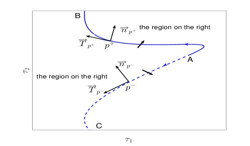
Figure 21: The positive direction and crossing direction of a part of stability switching curves corresponding to $\Omega_{j,n}=[a_{j,n},b_{j,n}]$.

Denote $\lambda=\sigma+i\omega$. Write (23) as

$${\rm Re}D_{n}(\lambda;\tau_{1},\tau_{2})+i{\rm Im}D_{n}(\lambda;\tau_{1},\tau_{2})=0.$$

From the implicit function theorem, $\tau_{1}$, $\tau_{2}$ can be expressed as functions of $\sigma$ and $\omega$, and if ${\rm det}\left(\begin{array}[]{cc}R_{1}&R_{2}\\ I_{1}&I_{2}\end{array}\right)=R_{1}I_{2}-R_{2}I_{1}\neq 0,$ we have

$$\Delta(\omega):=\left(\begin{array}[]{cc}\frac{\partial\tau_{1}}{\partial\sigma}&\frac{\partial\tau_{1}}{\partial\omega}\\ \frac{\partial\tau_{2}}{\partial\sigma}&\frac{\partial\tau_{2}}{\partial\omega}\end{array}\right)\arrowvert_{\sigma=0,\omega\in\Omega_{n}}=-\left(\begin{array}[]{cc}R_{1}&R_{2}\\ I_{1}&I_{2}\end{array}\right)^{-1}\left(\begin{array}[]{cc}R_{0}&-I_{0}\\ I_{0}&R_{0}\end{array}\right),$$ (43)

where

$$\dfrac{\partial{\rm Re}D_{n}(\lambda;\tau_{1},\tau_{2})}{\partial\sigma}|_{\lambda=i\omega}=\dfrac{\partial{\rm Im}D_{n}(\lambda;\tau_{1},\tau_{2})}{\partial\omega}|_{\lambda=i\omega}=R_{0},$$

$$\dfrac{\partial{\rm Re}D_{n}(\lambda;\tau_{1},\tau_{2})}{\partial\omega}|_{\lambda=i\omega}=-\dfrac{\partial{\rm Im}D_{n}(\lambda;\tau_{1},\tau_{2})}{\partial\sigma}|_{\lambda=i\omega}=-I_{0},$$

$$\dfrac{\partial{\rm Re}D_{n}(\lambda;\tau_{1},\tau_{2})}{\partial\tau_{l}}|_{\lambda=i\omega}=R_{l},\dfrac{\partial{\rm Im}D_{n}(\lambda;\tau_{1},\tau_{2})}{\partial\tau_{l}}|_{\lambda=i\omega}=I_{l},$$

with $l=1,2$. Here we do not consider the case that $i\omega$ is the multiple root of $D_{n}(\lambda;\tau_{1},\tau_{2})=0$, i.e., $\frac{dD_{n}(\lambda;\tau_{1},\tau_{2})}{d\lambda}\mid_{\lambda=i\omega}=R_{0}+iI_{0}\neq 0$, thus we have ${\rm det}\left(\begin{array}[]{cc}-R_{0}&I_{0}\\ -I_{0}&-R_{0}\end{array}\right)=R_{0}^{2}+I_{0}^{2}>0.$ Therefore, the sign of $\delta(\omega)={\rm det}\Delta(\omega)$ is decided by $R_{1}I_{2}-R_{2}I_{1}$. We can verify that $R_{1}I_{2}-R_{2}I_{1}\mid_{p^{\pm}}=\pm\omega^{2}|P_{2,n}\overline{P}_{3,n}-P_{0,n}\overline{P}_{1,n}|\sin\theta_{1,n}$. From $\theta_{1,n}(\mathring{\Omega}_{j,n})\subset(0,\pi)$, we have

$$\begin{array}[]{l}\delta(\omega\in\mathring{\Omega}_{j,n})\mid_{p^{+}}>0,~{}~{}\forall p^{+}\in\mathcal{T}_{j_{1},j_{2},n}^{+j},~{}{\rm and}~{}\delta(\omega\in\mathring{\Omega}_{j,n})\mid_{p^{-}}<0,~{}~{}\forall p^{-}\in\mathcal{T}_{j_{1},j_{2},n}^{-j},\end{array}$$

where $\mathring{\Omega}_{j,n}$ denotes the interior of $\Omega_{j,n}$.

      Lemma 4.

For any $j=1,2,\cdots,N$, we have

$$\delta(\omega\in\mathring{\Omega}_{j,n})>0,~{}~{}\forall(\tau_{1}(\omega),\tau_{2}(\omega))\in\mathcal{T}_{j_{1},j_{2},n}^{+j},~{}{\rm and~{}}\delta(\omega\in\mathring{\Omega}_{j,n})<0,~{}~{}\forall(\tau_{1}(\omega),\tau_{2}(\omega))\in\mathcal{T}_{j_{1},j_{2},n}^{-j}.$$

Thus, we can get a further conclusion which is more intuitive.

      Remark 8.

The region on the right of $\mathcal{T}_{j_{1},j_{2},n}^{+j}$ has two more characteristic roots with positive real parts, and the region on the right of $\mathcal{T}_{j_{1},j_{2},n}^{-j}$ has two less characteristic roots with positive real parts.

Appendix C The stability switching curves in Fig. 20 in section 4.3

Following the steps in A and B, we can draw all the stability curves on $(\tau_{1},\tau_{2})$ plane, and decide the crossing direction.

We can verify that $F_{0}(0)>0$ and $F_{0}(\omega)=0$ has four roots (see Fig. 22 a)). Thus the crossing set $\Omega_{0}=$ $\Omega_{1,0}\bigcup\Omega_{2,0}=[a_{1,0},b_{1,0}]\bigcup[a_{2,0},b_{2,0}]$$=[0.0636,0.1184]\bigcup[0.3781,0.5602]$. From (39) and (40), we can get the stability switching curves $\mathcal{T}^{1}_{0}$ corresponding to $\Omega_{1,0}$ which is shown in Fig. 22 b). To show the structure of stability switching curves and the crossing direction clearly, we take a part of curves of $\mathcal{T}_{0}^{1}$ near the origin (i.e. $\tau_{0}^{1(1)}$ in Fig. 22 b)) as an example, and draw the figure in Fig. 23 a). From bottom to top, it starts with a part of $\mathcal{T}_{0,0,0}^{-1}$, which is connected to $\mathcal{T}_{0,1,0}^{+1}$ at $b_{1,0}$. $\mathcal{T}_{0,1,0}^{+1}$ is linked to $\mathcal{T}_{1,1,0}^{-1}$ at $a_{1,0}$, which is again connected to $\mathcal{T}_{1,2,0}^{+1}$ at $b_{1,0}$ $\cdots$. The numerical results support the analysis result in (38). Similarly, the stability switching curves $\mathcal{T}^{2}_{0}$ corresponding to $\Omega_{2,0}$ are shown in Fig. 22 c). All the stability switching curves for $n=0$ are given by $\mathcal{T}_{0}=\mathcal{T}^{1}_{0}\cup\mathcal{T}^{2}_{0}$. We also draw the leftmost curve of $\mathcal{T}_{0}^{2}$ (marked $\tau_{0}^{2(1)}$ in Fig. 22 c)) in Fig. 23 b). In Fig. 23, the arrows on the stability switching curves represent their positive direction. From Lemma 4, we know that the regions on the right (left) of the solid (dashed) curves, which the black arrows point to, have two more characteristic roots with positive real parts.

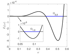
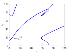
a) b) c)

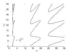
Figure 22: a) The crossing set $\Omega_{1,0}\bigcup\Omega_{2,0}$. b) Stability switching curves $\mathcal{T}^{1}_{0}$. c) Stability switching curves $\mathcal{T}^{2}_{0}$.

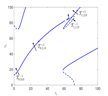
a) b)

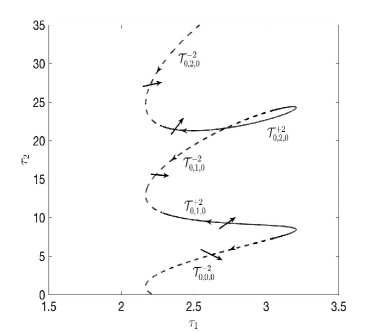
Figure 23: a) The detailed structure of $\tau_{0}^{1(1)}$ in Fig. 22 b). b) The detailed structure of $\tau_{0}^{2(1)}$ in Fig. 22 c).

When $n=1$, $F_{1}(0)>0$, and $F_{1}(\omega)=0$ has two roots. The crossing set $\Omega_{1}=$ $\Omega_{1,1}=[0.4149,0.5747]$, which is shown in Fig. 24 a). We can get the stability switching curves $\mathcal{T}^{1}_{1}$, which is shown in Fig. 24 b). Thus all the stability switching curves for $n=1$ are given by $\mathcal{T}^{1}_{1}$.

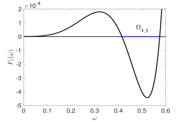
a) b)

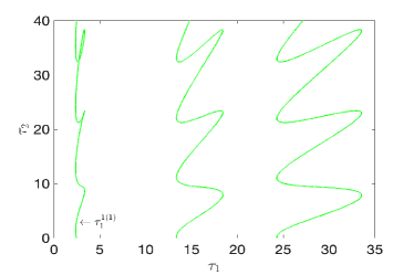
Figure 24: a) The crossing set $\Omega_{1,1}$. b) Stability switching curves $\mathcal{T}^{1}_{1}$.

When $n=2$, $F_{2}(0)>0$, and $F_{2}(\omega)=0$ has two roots, and the crossing set is $\Omega_{1,2}=[0.4304,0.5572]$, which is shown in Fig. 25 a). The stability switching curves $\mathcal{T}^{1}_{2}$ corresponding to $\Omega_{1,2}$ is shown in Fig. 25 b). All the stability switching curves for $n=2$ are given by $\mathcal{T}_{2}=\mathcal{T}^{1}_{2}$.

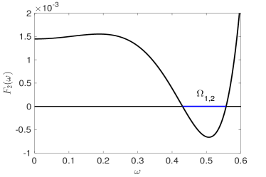
a) b)

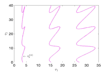
Figure 25: a) The crossing set $\Omega_{1,2}$. b) Stability switching curves $\mathcal{T}^{1}_{2}$.

When $n=3$, $F_{3}(0)>0$, and the crossing set such that $F_{3}(\omega)<0$ is $\Omega_{1,3}=[0,0.2348]$, which is shown in Fig. 26 a). And the stability switching curves $\mathcal{T}^{1}_{3}$ corresponding to $\Omega_{1,3}$ is shown in Fig. 26 b). Thus all the stability switching curves for $n=3$ are given by $\mathcal{T}_{3}=\mathcal{T}^{1}_{3}$.

When $n\geq 4$, $F_{n}(\omega)>0$ for any $\omega$, thus there are no stability switching curves on $(\tau_{1},\tau_{2})$ plane for $n\geq 4$.

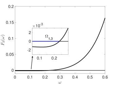
a) b)

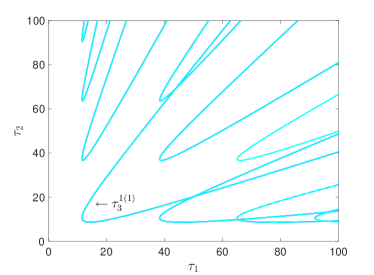
Figure 26: a) The crossing set $\Omega_{1,3}$. b) Stability switching curves $\mathcal{T}^{1}_{3}$.

Supplementary Material

In the supplementary material, we give the detailed calculation process of normal forms near double Hopf bifurcation induced by two delays.

References

C. Cosner, D.L. DeAngelis, J.S. Ault, D.B. Olson, Effects of spatial grouping on the functional response of predators, Theor. Popul. Biol. 56 (1999) 65-75.

J.M. Jeschke, M. Kopp, R. Tollrian, Predator functional responses: discriminating between handling and digesting prey, Ecol. Monogr. 72 ( 2002) 95-112.

C.S. Holling, The components of predation as revealed by a study of small-mammal predation of the european pine sawfly, Can. Entomol. 91(5) (1959) 293-320.

N.D. Kazarinov, P. van den Driessche, A model predator-prey system with functional response, Math. Biosci. 39 (1-2) (1978) 125-134.

P. Turchin, Complex Population Dynamics: A Theoretical/Empirical Synthesis, Princeton University Press, 2003.

P.A. Schmidt, L.D. Mech, Wolf pack size and food acquisition, Am. Nat. 150 (1997) 513-517.

F. Courchamp, D.W. Macdonald, Crucial importance of pack size in the African wild dog Lycaon pictus, Anim Conserv 4 (2001) 169-174.

D. Scheel, C. Packer, Group hunting behavioir of lions: a search for cooperation, Anim. Behav. 41 (1991) 697-709.

C. Boesch, Cooperative hunting in wild chimpanzees, Animal Behav. 48 (1994) 653-667

R. Bshary, A. Hohner, K. Ait-el Djoudi, H. Fricke, Interspecific communicative and coordinated hunting between groupers and giant moray eels in the Red Sea, PLoS Biol. 4 (12) (2006) e431.

G.W. Uetz, Foraging stratigies of spiders, Trends Ecol. Evol. 7 (1992) 155-159.

D. P. Hector, Cooperative hunting and its relationship to foraging success and prey size in an avian predator, Ethology 73 (1986) 247-257.

M.W. Moffett, Foraging dynamics in the group-hunting myrmicine ant, pheidologeton diversus, J. Insect Behav. 1 (3) (1988) 309-331.

L. Berec, Impacts of foraging facilitation among predators on predator-prey dynamics, Bull. Math. Biol. 72 (1) (2010) 94-121.

M.T. Alves, F.M. Hilker, Hunting cooperation and Allee effects in predators, J. Theor. Biol. 419 (2017) 13-22.

Sophia R.J. Jang, W.J. Zhang, V. Larriva, Cooperative hunting in a predator-prey system with Allee effects in the prey, Nat. Resour. Model. 31 (4) (2018) e12194.

S. Pal, N. Pal, S. Samanta, J. Chattopadhyay, Effect of hunting cooperation and fear in a predator-prey model, Ecol. Complex. 39 (2019) 100770.

D. Sen, S. Ghorai, S.M. Banerjee, Allee effect in prey versus hunting cooperation on predator-enhancement of stable coexistence, Int. J. Bifurcation Chaos 29 (6) (2019) 1950081.

S. Yan, D. Jia, T. Zhang, S. Yuan, Pattern dynamics in a diffusive predator-prey model with hunting cooperations, Chaos Solitons Fract. 130 (2020) 109428.

D.Y. Wu, M. Zhao, Qualitative analysis for a diffusive predator?prey model with hunting cooperative, Physica A 515 (2019) 299-309.

D.X. Song, C. Li, Y.L. Song, Stability and cross-diffusion-driven instability in a diffusive predator-prey system with hunting cooperation functional response, Nonlinear Anal. Real World Appl. 54 (2020) 103106.

W.C. Allee, The Social Life of Animals, William Heinemann, London, 1938.

F. Courchamp, L. Berec, J. Gascoigne, Allee Effects in Ecology and Conservation, Oxford University Press, Oxford, 2008.

J.F. Wang, J.P. Shi, J.J. Wei, Predator-prey system with strong Allee effect in prey, J. Math. Biol. 62(3) (2010) 291-331.

E.D. Conway, J.A. Smoller, Global analysis of a system of predator-Prey equations, SIAM J. Appl. Math. 46 (4) (1986) 630-642.

X. Lin, H. Wang, Stability analysis of delay differential equations with two discrete delays, Can. Appl. Math. Q. 20 (2012) 519-533.

M.L. Rosenzweig, R. MacArthur, Graphical representation and stability conditions of predator-prey interactions, Am. Nat. 97 (1963) 209-223.

M.L. Rosenzweig, Why the prey curve has a hump? Am. Nat. 103 (1969) 81-87.

S.B. Hsu, On global stability of a predator-prey system, Math. Biosci. 39 (1978) 1-10.

S. Wiggins, Introduction to Applied Nonlinear Dynamical Systems and Chaos, Texts Appl Math, vol 2, Springer, New York, 1990.

J.C. Alexander, J.A. Yorke, Global bifurcations of periodic orbits, Am. J. Math. 100 (1978) 263-292.

S.N. Chow, J. Mallet-Paret, The Fuller index and global Hopf bifurcation, J. Differential Equations 29 (1978) 66-85.

J. Wu, Symmetric functional-differential equations and neural networks with memory, Trans. Am. Math. Soc. 350 (1998) 4799-4838.

A. Dhooge, W. Govaerts, Y.A. Kuznetsov, MATCONT: a MATLAB package for numerical bifurcation analysis of ODEs, ACM Trans. Math. Softw. 29 (2003) 141-164.

J.A. Polking, D. Arnold, Ordinary Differential Equations Using MATLAB, 3rd edn. Prentice-Hall, Englewood Cliffs, 2003.

Y. Song, T. Zhang, Y. Peng, Turing-Hopf bifurcation in the reaction-diffusion equations and its applications, Commun. Nonlinear Sci. Numer. Simulat. 33 (2016) 229-258.

X. Xu, J. Wei, Turing-Hopf bifurcation of a class of modified Leslie-Gower model with diffusion, Disc. Continu. Dyn. Sys. B 23 (2018) 765-783.

Q. An, W. Jiang, Spatiotemporal attractors generated by the Turing-Hopf bifurcation in a time-delayed reaction-diffusion system, Discrete Contin. Dyn. Syst. B 24 (2) (2019) 487-510.

G. Guo, L. Liu, B. Li, J. Li, Qualitative analysis on positive steady-state solutions for an autocatalysis model with high order, Nonlinear Anal. Real World Appl. 41 (2018) 665-691.

Y. Kuang, Delay Differential Equations: with Applications in Population Dynamics, Vol. 191, Academic Press, 1993.

K. Gopalsamy, Stability and Oscillations in Delay Differential Equations of Population Dynamics, Vol. 74, Springer Science Business Media, 2013.

A. Martin, S.G. Ruan, Predator-prey models with delay and prey harvesting, J. Math. Biol. 43 (3) (2001) 247-267.

J. Xia, Z.H. Liu, R. Yuan, The effects of harvesting and time delay on predator-prey systems with Holling type II functional response, SIAM J. Appl. Math. 70 (4) (2009) 1178-1200.

E. Wright, A functional equation in the heuristic theory of primes, Math. Gaze. 45 (351) ( 1961) 15-16.

R.M. May, Time delay versus stability in population models with two and three trophic levels, Ecology 54 (2) (1973) 315-325.

C. Xu, X. Tang, M. Liao, X. He, Bifurcation analysis in a delayed Lokta-Volterra predator-prey model with two delays, Nonlinear Dyn. 66 (1) (2011) 169-183.

X.P. Yan, C.H. Zhang, Hopf bifurcation in a delayed Lotka-Volterra predator-prey system, Nonlinear Anal. Real World Appl. 9 (1) (2008) 114-127.

M. Jankovic, S. Petrovskii, Are time delay always destabilizing? Revisiting the role of time delays and the Allee effect, Theor. Ecol. 7(4) (2014) 335-349.

K.L. Cooke, P. van den Driessche, Analysis of an SEIRS epidemic model with two delays, J. Math. Biol. 35 (1996) 240-260.

H.I. Freedman, V.S.H. Rao, Stability criteria for a system involving two time delays, SIAM J. Appl. Math. 46 (1986) 552-560.

J.J. Wei, S.G. Ruan, Stability and bifurcation in a neural network model with two delays, Physica D 130 (1999) 255-272.

J. Xu, K.W. Chung, C.L. Chan, An efficient method for studying weak resonant double Hopf bifurcation in nonlinear systems with delayed feedbacks, SIAM J. Appl. Dyn. Syst. 6 (2007) 29-60.

Y.F. Du, B. Niu, J.J. Wei, Two delays induce Hopf bifurcation and double Hopf bifurcation in a diffusive Leslie-Gower predator-prey system, Chaos 29 (1) (2019) 013101.

C.X. Huang, Z.C. Yang, T.S. Yi, On the basins of attraction for a class of delay differential equations with non-monotone bistable nonlinearities, J. Differential Equations 256 (7) (2014) 2101-2114.

P. Yu, Y. Yuan, J. Xu, Study of double Hopf bifurcation and chaos for oscillator with time delay feedback, Commun. Nonlinear Sci. Numer. Simul. 7 (2002) 69-91.

Y.F. Du, B. Niu, Y.X. Guo, J.J. Wei, Double Hopf bifurcation in delayed reaction-diffusion systems, J. Dynam. Differential Equations 32 (2020) 313-358.

S. Ma, Q. Lu, Z. Feng, Double Hopf bifurcation for van der Pol-Duffing oscillator with parametric delay feedback control, J. Math. Anal. Appl. 338 (2008) 993-1007.

S.A. Campell, J. Bélair, T. Ohira, J.Milton, Limit cycles, tori, and complex dynamics in a second-order differential equations with delayed negative feedback, J. Dynam. Differential Equations 7 (1) (1995) 213-236.

J.H. Ge, J. Xu, An analytical method for studying double Hopf bifurcations induced by two delays in nonlinear differential systems, Sci. China-Technol. Sci. 63 (4) (2019) 597-602.

J. Wu, Theory and Applications of Partial Functional-Differential Equations, Springer, New York, 1996.

J. Hale, Theory of Functional Differential Equations, Springer-Verlag, 1977.

K.L. Cooke, Z. Grossman, Discrete delay, distributed delay and stability switches, J. Math. Anal. Appl. 86 (1982) 592-627.

S.G. Ruan, J.J. Wei, On the zeros of transcendental functions with applications to stability of delay differential equations with two delays, Dyn. Contin. Discret Impuls. Syst. Ser. A: Math. Anal. 10 (2003) 863-874.

T. Faria, Normal forms and Hopf bifurcation for partial differential equations with delays, Trans. Amer. Math. Soc. 352 (2000) 2217-2238.

J. Guckenheimer, P. Holmes, Nonlinear Oscillations, Dynamical Systems, and Bifurcations of Vector Fields, Springer, 1983.