Stochastic physics of species extinctions in a large population

Abstract

Species extinction is a core process that affects the diversity of life on Earth. Competition between species in a population is considered by ecological niche-based theories as a key factor leading to different severity of species extinctions. There are population dynamics models that describe a simple and easily understandable mechanism for resource competition. However, these models can not efficiently characterize and quantify new emergent extinctions in a large population appearing due to environmental forcing. To address this issue we develop a stochastic physics-inspired approach to analyze how environmental forcing influences the severity of species extinctions in such models. This approach is based on the large deviations theory of stochastic processes (the Freidlin-Wentzell theory). We show that there are three possible fundamentally different scenarios of extinctions, which we call catastrophic extinctions, asymmetric ones, and extinctions with exponentially small probabilities. The realization of those scenarios depends on environmental noise properties and the boundaries of niches, which define the domain, where species survive. Furthermore, we describe a hysteresis effect in species extinction showing that fluctuations can lead to dramatic consequences even if an averaged resource supply is sufficient to support population survival. Our stochastic physics-inspired approach generalizes niche theory by accounting environmental forcing and will be useful to find, by available data, which environmental perturbations may induce extinctions.

1 Introduction

Life on earth has co-evolved with fluctuations in both climate and the wider abiotic environment. However, the most pronounced changes in biota come during periods of extreme environmental perturbation. These are commonly associated with cataclysmic events (e.g. bolide impact) [1], rapid shifts in the climate state [2] or a combination of the the both factors [3]. During these periods the biotic and abiotic changes feedback on each other. Generally, the two-way interactions between populations in ecosystems and their abiotic characteristics have the potential to dramatically impact both biodiversity [4, 5, 6, 7, 8], and a wider planetary response to the changing environment [9, 10].

Mass extinctions represent important effects that correspond to biodiversity loss, ecosystem upheavals and changes to the evolution of life. This is seen in the fossil record through pronounced changes in fossil assemblages with mass extinctions being attributed to large-scale environmental disasters [11]. However, their dynamics are often poorly understood: it is often unclear as to why populations decline to the point of a species becoming extinct. Here we assess a generic range of environmental forcing types and its impact on the dynamics of species extinction and evolution. These forcing characteristics are macroscopic and emergent properties of small scale wave interaction processes for the ocean - atmosphere - land system.

Some studies [4, 6, 7] show that extinctions play a major role in maintaining population dynamics for niche species due to the niche-overlap in growing species populations increases and co-existence becomes more uncertain [12]. Employing stochastic physics is a perspective way to develop a better understanding of how the scenarios of extinction depend on environmental fluctuation features and the boundaries of niches. In this paper, we develop an approach based upon recent studies investigating the connection between ecological dynamics in a changing environment and the statistical/stochastic physics of large systems [13, 14, 15, 16, 17, 18]. However, in contrast to these previous works, we propose to study the multistability effect in a system with a large population and fixed parameters replacing it to a similar system with slowly evolving parameters and observable jumps between equilibria. This technique is originally proposed in the large deviations theory of stochastic processes and has been introduced in the work of M. Freidlin and A. Wentzell [19].

We propose a general s stochastic population competition model that allows the assessment of how a wide range of environmental forcing types can affect biodiversity (the number of coexisting species), biomass (the number of species in a population) and extinction. In that model, extinctions are inevitable if a population has the maximal possible biodiversity and uses the maximal amount of resources. Also, we use fairly general assumptions. First, each species can survive within a niche, so-called Hutchinsonian niche in environmental parameter space [20]. That niche is an ”n-dimensional hypervolume”, where the dimensions are environmental conditions and resources. Furthermore, dynamics of environmental forcing is defined by stochastic dynamical systems with a small noise. Then we show that there exist three different regimes of extinctions: all species become extinct in a very fast way, all species become extinct very slowly, or part of the species become extinct quickly with the remaining ones slowly. The occurrence of the situations depends on mutual location of the system attractors that define the environmental forcing type and species niches.

We use a general range of environmental forcing types: time quasiperiodic oscillations, a simple white noise, and chaotic dynamics with many attractors and a weak noise. We assume that such changes in the environment may influence the states of the system of species. Indeed, in the Earth’s climate system there is the El Niño-Southern Oscillation (ENSO), short term ($3$ to $10$ year) cycles of nonlinear interaction of wind with the equatorial waveguide in the Pacific. There are many shreds of evidence that this phenomenon affects the ecosystems as a form of chaotic forcing effect [21]. These chaotic and stochastic effects can occur due to turbulence and small scale wave interaction processes in the surface wind stress and internal ocean and that these can play an important role in climate [22, 23]. When a system exhibits periodic forms of chaos, the stochastic nature of the system leads to eigenmode repulsion: the spacing between adjacent eigenmodes follows a universal Gaussian ensemble and Random Matrix Theory (RMT) [23] is used to identify these stochastic system types by assessing emergent resonance phenomena. It helps to reveal how internal system wave mechanisms interact and so influence the ecosystems in their vicinity.

The paper is organized as follows. In Section 2 we state the niche model of species coexistence and we describe different models of environment fluctuations. In Section 3 we explain our main result: the description of general different extinction scenarios. In this section the Freidlin-Wentzell theory [19] is applied to describe influences of a weak noise (which is further outlined in the Appendix). In Section 4 we study the extended dynamical model of a population competing for resources [24, 25, 26, 27], which takes into account species extinctions and time oscillations of the resource. This model is an extension of the well-known J. Huisman and F. Weissing model [24] that has been used to study phytoplankton. The model accounts for species self-regulation, extinctions, and time dependence of resources. For large resource turnovers this model has a simple asymptotic solution. Section 5 discusses the qualitative processes of the extinction in a population dynamics model. In Section 6 we describe the results of numerical simulations.

2 Niche model and environmental fluctuations

We consider a system of species that depend on the environmental state $q$. For example, plants or plankton species depend on a few of resources, and certain resources are directly connect with the environment (sun light, temperature, $CO_{2}$ concentration etc.). To do this we utilize the ideas of niche theory [15]: a $j$-th species survives only when environment parameters lies within a given domain denoted by $\Omega_{j}$.

Let us suppose that a system occupies a specific area or region. We denote the averaging over that area as well as the environmental parameters (which are essential for species survival) by $(q_{1},q_{2},...,q_{n})=q\in{\mathbb{R}}^{n}$. This property can also be time $t$ dependent. The key specification for niche survival is that the $j$-th species survives while $q(t)\in\Omega_{j}$. Each domain (niche) $\Omega_{j}$ is a bounded subset of ${\mathbb{R}}^{n}$ with a smooth boundary $\partial\Omega_{j}$. In this model, extinctions occur when $q$ goes through the boundary $\partial\Omega_{j}$ for certain $j$ and leaves the domain $\Omega_{j}$. We define a mass extinction as occurring when $q$ leaves a number of the domains $\Omega_{j}$ within a specific time period.

The generic form of environmental forcing $q$ reveal how internal system wave mechanisms interact and so influence species in their vicinity. These environmental forcing and species response impacts range from oscillatory, chaotic and noisy-stochastic physical perturbations. Our specification here accommodates these entire range of perturbation types. Periodic and quasiperiodic environmental oscillations and stochastic effects can also also impact the extreme range leading to perturbations in species which can subsequently exhibit this a non-linear and chaotic responses [21, 22, 23, 28]. When a system exhibits periodic forms of chaos, the fundamental random and stochastic nature of the system leads to eigenmode repulsion: the spacing between adjacent eigenmodes follows a universal Gaussian ensemble. In that setting including RMT provides the ability to assess emergent species survival properties [23].

In all cases, we suppose that the system depends on environment state via the resource supply

$$S=\bar{S}+\tilde{S}(q(\tau)),$$ (1)

where the perturbation $\tilde{S}$ of the background resource supply $\bar{S}$ and dynamics of the environment state $q$ is slow, i.e., $\tau=\kappa t$, $\kappa<<1$. In this work we assess scenarios of extinction under noise. This includes the range of environmental forcing types given below, which provide a range of forcing types from oscillatory motion, noisy systems to a non-linear chaotic forcing type that accommodates all the oscillatory and noisy settings.

2.1 Periodic and quasiperiodic variation

The simplest model, that simulates the effect induced by large scale environmental forcing scenarios [21], is

$$q(\tau)=q^{0}+Re\ \sum_{j=1}^{m}c_{j}\exp(i\omega_{j}\tau),$$ (2)

where $q^{0}$ is a constant, $i=\sqrt{-1}$, $c_{j}$ are coefficients and $\omega_{j}$ are frequencies (periodic and/or quasiperiodic oscillations). Model (2) can be extended to include a very slow variation or trend as

$$q(\tau)=q^{0}+\alpha\tau+Re\ \sum_{j=1}^{m}c_{j}\exp(i\omega_{j}\tau).$$ (3)

2.2 Dynamical forcing with noise

Where the dynamics of $q$ is governed by trajectories of a noisy dynamical system, we write this in the Ito form

$$dq=Q(q)d\tau+\sqrt{\epsilon}\ dB(\tau),$$ (4)

where $B(t)$ is the standard Brownian motion and $Q$ is a smooth vector field, $\epsilon>0$. In the case $\epsilon=0$ the system explanation reduces to the differential equation

$$\frac{dq}{dt}=Q(q),$$ (5)

and we suppose that its dynamics are well posed and this has a compact attractor ${\mathcal{A}}_{Q}$. By varying different $Q$, we can obtain different kinds of noise induced forcing. The emergent RMT properties are a feature of such noise induced systems. In this noisy type where small $\epsilon>0$ we can also apply the Freidlin-Wentzell theory [19] and also see the Appendix.

2.3 Bistable state transitions

The generic model we select to represent bistability is obtained by setting $q\in{\bf R}$ and $Q=aq-q^{3}$, where $a$ is a parameter. For $a>0$ the attractor consists of two stable points, $q=\pm a^{-1/2}$. In noisy systems, this system exhibits random transitions from state $q=1$ to state $-1$ and back. By varying the size of $\epsilon$ the occurrence of such transitions can be regulated, for small (large) $\epsilon$ these transitions are rare (frequent), see Figure 1.

Figure 1: This plot shows Kramers transitions for model from subsection 2.3. We set $Q=q-q^{3}$, $q\in{\bf R}$ and the noise $B(t)$ is a sequence of random outliers. For each time $t$ we have either $B(t)=r$ with probability $p_{out}$ (where $r$ is a random number) or otherwise $B(t)=0$. We sample $r$ from the normal distribution, $r\in{\bf N}(0,3)$.

2.4 Chaotic forcing

A generic representation of chaotic forcing is the non-linear delay oscillator. This model is

$$\frac{dq}{d\tau}=aF(q(\tau-\tau_{1}))-aF(q(\tau-\tau_{2}))+c\cos(\omega\tau),$$ (6)

where $a,b,c,\tau_{k}$ are positive and non-linearity $F$ can be chosen, for example, in the form $F(q)=q-q^{3}$. This accommodates regular seasonal forcing, non-linear wave interaction processes and time delays and it is discussed in detail in [21]. This type of forcing generically corresponds to a periodic map, with universal properties for this established by Feigenbaum [29]. It is a model for cascades into turbulence and sub-harmonic resonance that applies to all such periodic map processes. This chaotic forcing exhibits high frequency intermittency [21] and slow variation modes consistent with centennial time scales [30]. This dynamic model has a wide range of properties and used to represent the generic wave-interaction ENSO process. It can be used to move through states of oscillatory motion, bifurcations, chaos and intermittency. Periodic map properties also occur for species [5].

3 The scenarios of extinction under environmental forcing

Our primary goal is to find the probabilities of extinctions in our model. We consider three sharply different extinction scenarios of this which can be generated by random and non-random environment forcing induced by equation (5). Using the well known results [19] (see Appendix) we establish that there are three possible extinction scenarios as a function of the noise magnitude $\epsilon$ and mutual locations of the sets ${\mathcal{A}}_{Q}$ and $\partial\Omega_{j}$. Let us remind that ${\mathcal{A}}_{Q}$ denotes an attractor of dynamical system (4) for $\epsilon=0$ and $\partial\Omega_{j}$ denotes a boundary of existence of $j$-th species in the space parameter. In our model , that boundary is defined by the resource supply $S=S(q)$, where $q$ evolves according to (4). Let us denote by $P_{j,\epsilon}$ the probability of extinction of the $j$-th species per a fixed time period (here $\epsilon$ is the noise level, see the previous section).

By arguments stated in Appendix we find the following three sharply different scenarios of extinction types:
 
I. Catastrophic species extinctions: If the intersection $I={\mathcal{A}}_{Q}\cap{\partial\Omega}_{j}$ is not empty for all $j=1,...,k$ then the probability $P_{j,\epsilon}$ is not exponentially small, i.e., $\lim_{\epsilon\to 0}\epsilon\log P_{j,\epsilon}>0$. It is a catastrophic scenario when the extinction of all species (mass extinction) is quite probable.
 
II. Species extinctions with exponentially small probabilities: The intersection $I={\mathcal{A}}_{Q}\cap{\partial\Omega}_{j}$ is empty for all $j$. Then the probabilities $P_{j,\epsilon}$ are exponentially small both for large and small extinctions.
 
III. Asymmetric species extinctions: The intersection $I={\mathcal{A}}_{Q}\cap{\partial\Omega}_{j}$ is not empty for some $j$ but it is empty for others $j$. Then it is possible that the probability $P_{j,\epsilon}$ is not small for extinctions involving relatively few species but that probability is exponentially small for extinctions involving relatively many species. In this case, there is a sharp transition in the probabilities of small losses of biodiversity and great losses of biodiversity.
 
When the attractor consists of $n_{A}>1$ connected components ${\mathcal{A}}_{Q}^{(i)}$ we find that there are possible additional effects that may be caused by bifurcations in the environment system. For example, some climate models exhibit a possibility of climate bifurcations (tipping points) [31, 32] with rapid changes of the climate system from one stable state to another. With the non-linear delay oscillator dynamic (3) and (6) transitions from rapidly varying intermittent to slowly modulated cyclic forcing can be accommodated [21]. The species resilience impact of these three extinction types may correspond to a variation between system state [5]. One can suppose that the climate bifurcations may be caused by a transition from a connected component to another one: for example, by a transition from scenario I to scenario II (or III), and vice versa. Overall we can say that extinctions in such models are completely predetermined by the distances between the local attractors of the noisy dynamical systems that generates the environmental forcing and critical resource level sets. It is worth noting that among the variants considered in subsection 2.4 the most interesting case is defined by the equation (6), which provides a framing to encapsulate all the scenarios of interest.

4 The resource model

We consider the following standard model of biodiversity [24]:

$$\frac{dx_{i}}{dt}=x_{i}(-r_{i}+\rho_{i}(v)-\sum_{j=1}^{N}\gamma_{ij}\;x_{j}),$$ (7)

$$\frac{dv}{dt}=D(S-v)-\sum_{j=1}^{N}c_{j}\;x_{j}\;\rho_{j}(v),$$ (8)

where

$$\rho_{j}(v)=\frac{a_{j}v}{K_{j}+v},\quad a_{j},\ K_{j}>0,$$ (9)

are Michaelis-Menten’s functions, $x_{i}$ are species abundances, $r_{i}$ are the species mortalities, $D$ is the resource turnover rate, $S$ is the supply of resource $v$, and $c_{i}$ is the content of the resource in the $i$-th species. These constants define how different species share resources. Note that if $c_{i}=0$ then the equation for $v$ becomes trivial and $v(t)\to S$ for large times $t$, i.e., the resource equals the resource supply. The terms $\gamma_{ii}x_{i}$ define self-regulation of species populations that restrict the species abundances, and $\gamma_{ij}x_{j}$ with $i\neq j$ define a possible competition between species for resources. The coefficients $a_{i}$ are specific growth rates and the $K_{i}$ are self-saturation constants. If $\gamma_{ij}=0$ this system is equivalent to those in works where the plankton paradox [33] is studied. For the case of $M$ resources we have more complicated equations

$$\frac{dx_{i}}{dt}=x_{i}(-r_{i}+\phi_{i}(v)-\sum_{j=1}^{N}\gamma_{ij}\;x_{j}),$$ (10)

$$\frac{dv_{j}}{dt}=D_{j}(S_{j}-v_{j})-\sum_{k=1}^{N}c_{jk}\;x_{k}\;\phi_{k}(v),$$ (11)

where $v=(v_{1},v_{2},...,v_{M})$, and

$$\phi_{j}(v)=\min\{\frac{a_{j}v_{1}}{K_{1j}+v_{1}},...,\frac{a_{j}v_{M}}{K_{Mj}+v_{M}}\}\,.$$ (12)

with $a_{j}$ and $K_{ij}>0$. This model is widely used for primary producers like phytoplankton and it can also be applied to describe competition for terrestrial plants [34]. Relation (12) corresponds to the von Liebig minimum law, but we can consider even more general $\phi_{j}$ satisfying the conditions

$$\phi_{j}(v)\in C^{1},\quad 0\leq\phi_{j}(v)\leq C_{+},$$ (13)

where $C_{+}>0$ is a positive constant, and

$$\phi_{k}(v)=0,\quad\forall k\quad v\in\partial{\bf R}^{N}_{>}$$ (14)

where $\partial{\bf R}^{N}_{>}$ denotes the boundary of the positive cone ${\bf R}^{N}_{>}=\{v:v_{j}\geq 0,\ \forall j\}$. Note that condition (14) holds if $\phi_{j}$ are defined by (12). Similarly as above, we assume that $\sum_{k=1}^{N}c_{ik}=1,\quad c_{ik}>0.$ This model is well posed. Under certain natural conditions to $\gamma_{ij}$ solutions are defined for all positive times $t$, they are unique and there exists a finite dimensional attractor [25].

5 The hysteresis effect

Suppose the resource supply $S$ depends on an external parameter, for example, temperature, $T$, which evolves very slowly through a long term Ocean basin scale mode [21, 30] or similar slowly varying environmental process. Bruun et al. [21] showed that at a Pacific basin scale the tree-growth and temperature hysteresis exhibited persistent cycles that contributed to epochs of excessive heat and cold over a seven century time period. That work showed that the cyclic modes became unstable at the extreme range of the hysteresis curve, however those modes stayed stable overall, and indicated that the current warming period is at the hysteresis upper thermal edge for environmental forcing dynamics.

It is natural to suppose that at each $T$ our system in an equilibrium state. Let $S(T)$ be an increasing function of $T$. Then as $T$ increases from $T_{0}$ up to $T_{1}>T_{0}$ we can observe a bifurcation sequence described in the previous subsection. In our model we obtain that our system is, in sense, invertible, i.e., as $T$ changes from $T_{1}$ to $T_{0}$, we observe the same bifurcations but going in the reverse order. Thus, in our ideal model slow environmental oscillations do not affect biodiversity. However, in a more realistic situation, where species extinct if their abundance is less than a certain threshold $X_{ext}$ (this model is considered in [25] in another context), then environmental oscillations can lead to partial loss of species. In our model by letting $T$ slowly go from $T_{1}$ to $T_{0}<T_{1}$ so that for the abundance of a species at $T=T_{0}$ falls beneath the threshold, then this species never returns in our system, even when $T$ returns to the start value $T=T_{1}$. This effect is illustrated by the Figure 2.

Figure 2: The representation of an extinction process. Each cycle of change of resources supply from $S_{1}$ to $S_{0}$ and back leads to a decrease in species number $N$. As a result, a population may become extinct.

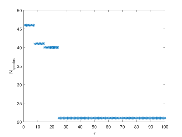
Figure 3: This plot shows as noisy environmental forcing can lead to extinctions. Here we do not take into account hysteresis, i.e., we suppose that population restores after each environmental shock (the time like parameter $\tau$ numerates shocks). We consider an equilibrium state for standard model (10, 11) with a single resource and the number of species $N_{species}$ coexisting in that equilibrium state. The model parameters are: initial species number $N_{pool}=50$, $b_{i}=2$, $K_{i}=4$, where $i=1,...,N_{pool}$, $D=5$, and $S=10$. The mortalities $r_{i}$ are independent random numbers distributed normally according to ${\bf N}(1,0.1)$. The matrix $\gamma_{ij}$ is diagonal with entries $\gamma_{ii}=1$. The noise is induced by random outliers of $S$ at times $t=\tau,2\tau$ … where $\tau>>1$. These outliers are defined by so $S(\tau)=\bar{S}+\tilde{S}(\tau)$, where $\tilde{S}(\tau)$ are independent random numbers normally distributed according to ${\bf N}(0,3)$ and $\bar{S}=10$.

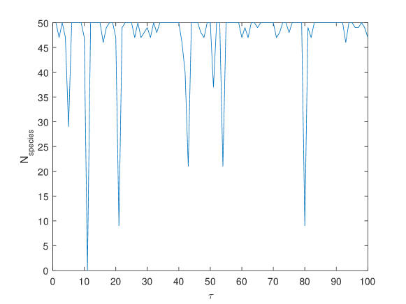
Figure 4: Noisy environmental forcing leading to extinctions. Here we take into account hysteresis, i.e., we suppose that population does not restore after each environmental shock. We consider an equilibrium state for the standard model with a single resource and the same parameters as on the previous image.

5.1 Analytical study of hysteresis in noisy environment

To investigate hysteresis effect, we consider the simplest case of model (7,8) with a diagonal matrix $\gamma_{ij}=\delta_{ij}\gamma$, identical parameters $K_{i}=K$ and $b_{i}=b$ and random mortalities $r_{i}$, which are random positive numbers distributed according to a density $\rho(r)$. Moreover, let $c_{k}=c>0$. Then it is natural to introduce notation $\phi(v)=bv/(K+v)$. For fixed $S$ and large $D$ the system is in an equilibrium state defined by [25]

$$D(S-v_{eq})=cB_{M}\;\phi(v),$$ (15)

where

$$B_{M}=\sum_{k=1}^{N}X_{k}(v_{eq})$$

is a biomass of the system and

$$X_{k}=\gamma^{-1}(\phi(v_{eq})-r_{k})_{+}$$

are steady state species abundances and $f_{+}=\max\{0,f\}$.

We consider the following simple model of noise in $S$. Suppose at certain moments $\tau_{j}=j\Delta t$ we have jumps in $S$: $S(\tau_{j}+0)=S(\tau_{j}+0)+\Delta S_{j}$, those outliers $\Delta S_{j}$ can have different signs. Moreover, we assume that the interval $\Delta t$ is much more than the characteristic relaxation time $t_{eq}$, thus most of the time within the interval $I_{j}=[\tau_{j},\tau_{j+1})$ system (7), (8) is an equilibrium state corresponding to the resource supply value $S(\tau_{j}+0)=S+\Delta S_{j}$. At initial time moment we have a pool of species with $N=N_{pool}>>1$ of species. Let $N_{sp}(\tau_{j})$ be the number of species with non-zero abundances at $t\in(\tau_{j},\tau_{j+1})$, i.e, biodiversity within the interval $I_{j}$. Then for the number $N_{sp}$ one has the following recurrent relation:

$$N_{sp}(\tau_{j+1})=N_{sp}(\tau_{j})\mu_{j}$$

where $\mu_{j}$ is a fraction of species, which survive after $j$-th outlier. For $N_{sp}>>1$ this fraction can be estimated as follows. Note that if $k$-th species survives, i.e. $X_{k}(v_{eq})>0$ then $r_{k}>\phi(v_{eq})$. The value $v_{eq}$ increases in $S$. Let us denote by $V_{j}$ the equilibrium value $v_{eq}$ for $t\in[\tau_{j-1},\tau_{j})$. For $\Delta S_{j}\geq 0$ one obtains that $\mu_{j}=1$. For $\Delta S_{j}<0$ one has

$$\mu_{j}\approx\frac{\int_{-\infty}^{\phi(V_{j+1})}\rho(r)dr}{\int_{-\infty}^{\phi(V_{j})}\rho(r)dr}$$

Consider the sequence of $S(\tau_{j})$, $j=1,...,N_{S}$. This sequence can be decomposed into increasing and decreasing sub-sequences. Similarly, the corresponding sequence of equilibrium values $V_{j}$ falls into analogous increasing and decreasing sub-sequences since $v_{eq}(S)$ is a monotone increasing in $S$ function. As $S$ non-decreases, the population diversity conserves and all species survive. Thus increasing intervals change nothing in diversity. Consider a decreasing interval, which starts with $S=S_{b}$, and finishes at a local minimum of $S$, which equals $S_{e}$. A change in species diversity within such decreasing interval is defined then by

$$\frac{{N_{sp}}^{(e)}}{{N_{sp}}^{(b)}}\approx\frac{\int_{-\infty}^{\phi(V_{e})}\rho(r)dr}{\int_{-\infty}^{\phi(V_{b})}\rho(r)dr},$$

where ${N_{sp}}^{(b)}$ and ${N_{sp}}^{(e)}$ are diversities at the beginning and the end of the decreasing interval, and $V_{e},V_{b}$ are equilibrium value of $v$ at the beginning and the end of the decreasing interval. For all the period of evolution one has

$$N_{sp}^{(f)}\approx N_{sp}(0)\Big{(}\int_{-\infty}^{\phi(V_{min})}\rho(r)dr\Big{)}\Big{(}\int_{-\infty}^{\phi(V_{0})}\rho(r)dr\Big{)}^{-1},$$ (16)

where $N_{sp}^{(f)}$ is a final diversity value and $V_{0}$ is the initial equilibrium value of $v$.

Under certain assumptions, this formula can be generalized for the multi-resource case. Again, let $\phi_{i}(v)=\phi(v)$ be the same for all species, but mortalities $r_{i}$ could be different. The main additional assumption is that turnovers $D_{i}>>1$. Then one can show that the attractor of system (10), (11) is a stable equlibria, and equilibrium value of $v_{i}$ are close to the corresponding resource supplies $S_{i}$. Then, by the same arguments, we obtain

$$N_{sp}^{(f)}\approx N_{sp}(0)\Big{(}\int_{-\infty}^{\phi_{min}}\rho(r)dr\Big{)}\Big{(}\int_{-\infty}^{\phi(S(0))}\rho(r)dr\Big{)}^{-1},$$ (17)

where $S=(S_{1},S_{2},...,S_{M})$ is the vector of resource supplies, $S(0)$ is an initial value of that vector and $\phi_{min}$ is the minimal value of $\phi(S)$ on the whole evolution time interval. In other situations the problem is much more complicated, and it will be considered in future studies.

6 Simulations for simplest model

Numerical simulations are made for the simplest model with a single resource considered in the previous section. We use the formula (15). We suppose that at initial time moment we have $50$ coexisting species and the parameters are $N_{pool}=50$, $b_{i}=2$, $K_{i}=4$, where $i=1,...,N_{pool}$, $D=5$, and $S=10$. The mortalities $r_{i}$ are independent random numbers distributed normally according to ${\bf N}(1,0.1)$. The matrix $\gamma_{ij}$ is diagonal with entries $\gamma_{ii}=1$. To assess the species model characteristic we considered the perturbations of $\tilde{S}(q(\tau))$ defined by different models: the periodic and quasiperiodic one defined by (3), a purely random model with $q(\tau)=B(\tau)$ and $B(t)$ is a white noise, the model exhibiting the Kramers transitions from Subsection 2.3 and the chaotic forcing (6). The results of simulations are presented in Figures 3 and 4.

To compare our results, we consider perturbations of $\tilde{S}$ of the same amplitude normalized as follows:

$$\tilde{S}(q(\tau))=\epsilon(q(\tau)-\bar{q})/var(q),$$

where $\bar{q}$ is the mean over trajectories $q(\tau)$, and $var(q)=\max q(\tau)-\min q(\tau)$. We have made $50$ tests for each perturbation with random mortalities and random $q(t)$, where $\epsilon=5$ and $\bar{S}=10$. Using the test simulation ensemble we compute the number of extinctions $n_{ext}$, the number $N_{surv}$ of finally survived species, the mean size of extinctions $\bar{N}_{ext}$ and maximal size $\bar{N}_{ext,max}$ of extinctions.

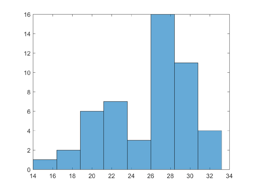
(a)

(b)

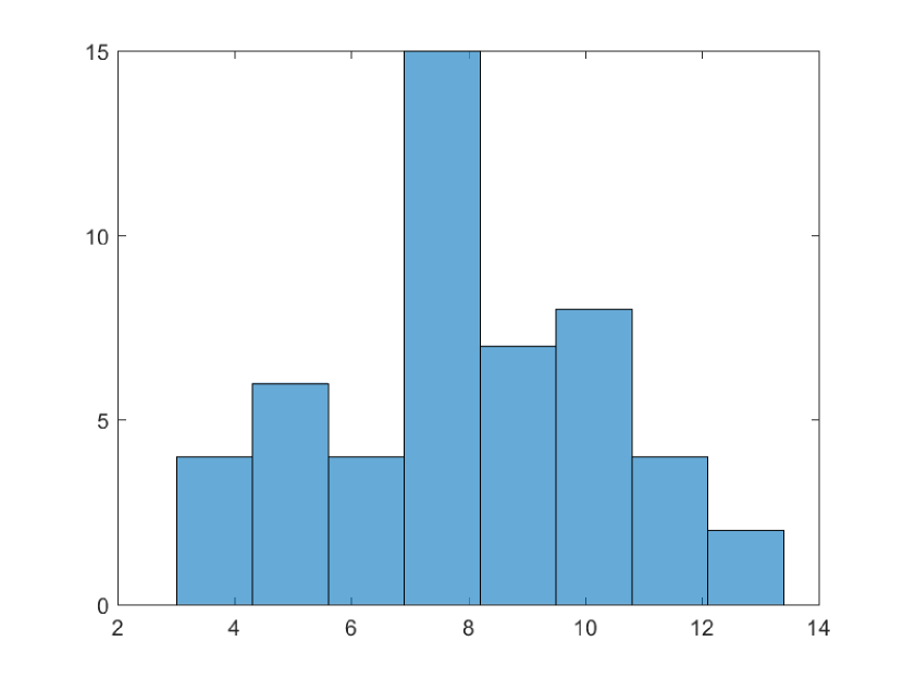
(c)

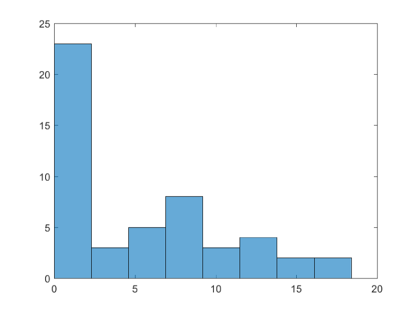
(d)

Figure 5: (a) The histogram for the number of extinctions within the period evolution $15000$ steps for periodic perturbations (3) with two different small frequencies $\omega_{1}=0.01,\omega_{2}=0.03$ and with $c_{1}=1,c_{2}=0.5$ (simulation uses (15) and parameters here for all plots are as for Fig. 3). (b) This plot shows the histogram for the number of extinctions within the period evolution $15000$ steps under a random white noise perturbation. (c) This plot shows the histogram for the number of extinctions within the period evolution $15000$ steps under a perturbation (Subsection (2.3)), where $a=1$, and it is perturbed by random uniformly distributed outliers of frequency $p_{out}=0.1$ so that system for $q$ exhibits the rare Kramers transitions from $q_{1}=\pm 1$ to $q_{2}=-q_{1}$. (d) This plot shows the histogram for the number of extinctions within the period evolution $15000$ steps for perturbations (6) with the frequency $\omega=0.01$ and $a=0.1,c=0.2$.

Results for the number of extinctions are shown on Figure 5. The distributions of the number of extinctions $n_{ext}$ are essentially different for different cases. For the plots (a) and (b) on Figure 5 it was checked by the Kolmogorov-Smirnov test. For the mean extinction size $\bar{N}_{ext}$ we obtain the following. In quasiperiodical case $\bar{N}_{ext}\approx 1$, for purely random perturbations $\bar{N}_{ext}\approx 2.7$, for model from Subsection 2.3 $\bar{N}_{ext}\approx 2.0$, and for the model (6) one has $\bar{N}_{ext}\approx 3.0$. By the end of evolution ($15000$ steps) $14$ species survived in the periodical case, $17$ in purely random case, and $14$ species survived for the model (6) and $16$ for the model with the Kramers transitions. We can conclude that the number of survived species on a long period depends on average intensity of environment perturbations but statistics and the size of extinctions depend on perturbation type. The periodic and chaotic forcing pertubation types, associated with periodic attractor and Gaussian ensemble eigenmode interaction type [21, 23] giving lower species survival. This type of interacting eigenmode environment perturbation may act to constrain the biota diversity accordingly.

7 Conclusions

In this paper, using a fairly general niche model and the large deviations theory of stochastic processes, we show that there are possible three fundamentally different extinction scenario types that can be distinguished based on a state of the environment. To demonstrate the applicability of the proposed ideas we employ a resource model that describes a simple and easily understandable mechanism for resource competition in a population and takes into account species self-regulation, extinctions, forcing of the environment and time dependence of resources.

The main result is that chaotic forcing perturbations can essentially affect biodiversity through a hysteresis effect for species extinctions. Different types of noise are considered, and it is found that the extinction probability sharply depends on the form of a noisy process. We also show that some environmental fluctuations may lead to dramatic consequences even if an averaged resource supply is sufficient to support population survival. In this case, the population can be destroyed by environmental noises. It is important to establish how many local attractors are generated by the internal wave interactions of the dynamical systems that defines environmental forcing and the location of these attractors with respect to critical level sets for resource supply. The periodic and chaotic forcing systems used here can exhibit eigenmode level repulsion that places the system in a chaotic class known as a Gaussian ensemble [23].

This work contributes to the statistical physics of the ecological niche theory. The key works in this area [16, 17, 18] demonstrate that stochastic processes can induce phases transitions in population from a niche phase where species competitions define the dynamics of the system to a neutral phase where stochasticity is the main driver of the population dynamic. Our results show that the behavior of niche and neutral models is quite different when we take into account the environmental fluctuations.

In addition, our results can be interesting for the biodiversity problem. A globally prevalent generalist species like plankton may benefit from the effects of periodic and chaotic environmental forcing [7] which enables it to adapt and out-compete other species by providing and ecosystem resilience when faced with system state changes. We also think that our results will be applicable to the studies of past mass extinctions because recently such extinctions are considering as phases of a natural, ’meta-evolution’ quasi-cycle where the timing and magnitude of mass extinctions are essentially stochastic events [35].

Appendix

Here we outline the Freidlin-Wentzell theory. Let the set of all possible trajectories $p(t)\ t\in[0,T]$ defined on the time interval $[0,T]$ be equipped by the standard norm $||\cdot||_{\infty}$. Then the set of trajectories with bounded norm $||\cdot||_{\infty}$ becomes a Banach space, which will be denoted ${\mathcal{B}}_{T}$.

Following [19] we define the rate function $I(q(\cdot))$, defined on the set of the trajectories $q(\cdot)$ by

$$I(q(\cdot))=\frac{1}{2}\int_{0}^{T}|\frac{dq(t)}{dt}-Q(q(t)|^{2}dt.$$ (18)

For each closed subset ${\mathcal{S}}\subset{\mathcal{B}}_{T}$ of trajectories let us consider the quantity

$$P_{\mathcal{S}}=\inf_{q\in{\mathcal{S}}}I(q(\cdot))$$

where we take the infimum over all possible trajectories belonging to ${\mathcal{B}}_{T}$, which lie in the set ${\mathcal{S}}$ for each $t\in[0,T]$. Then, according to [19] one has

$$\liminf_{\epsilon\to 0}\epsilon\ln Prob\{q\in{\mathcal{S}}\}\leq-P_{\mathcal{S}}$$ (19)

and

$$\limsup_{\epsilon\to 0}\epsilon\ln Prob\{q\in{\mathcal{S}}\}\geq-P_{\mathcal{S}}.$$ (20)

Let us define the distance $d(q,q^{\prime})$ between two points $q$ and $q^{\prime}$ by

$$d_{FW}(q,q^{\prime})=\frac{1}{2}\inf_{p(\cdot)\in B(q,q^{\prime})}I(p(\cdot)).$$

where we take the infimum over the set $B(q,q^{\prime})$ of the trajectories $p(t)$ such that $p(0)=q$ and $p(T)=q^{\prime}$ and over all $T>0$.

The distance between the two sets $A$ and $B$ is defined as $dist(A,B)=\inf_{q\in A,q^{\prime}\in B}d_{FW}(q,q^{\prime})$. The main property of $dist(q,q^{\prime})$, needed for us, we use is as follows.

The probability $P_{c,\epsilon}$ to attain the critical value starting from a point on a local attractor ${\mathcal{A}}_{Q}$ satisfies the estimate

$$\lim_{\epsilon\to 0}\epsilon\log P_{j,\epsilon}=-\inf_{q\in{\mathcal{A}}_{Q},q^{\prime}\in{\mathcal{O}}({\Delta S}_{j})}d_{FW}(q,q^{\prime}).$$ (21)

By the definition of $dist(q,q^{\prime})$ it is easy to show that if $q$ is a starting point of a trajectory of our dynamical system leading to $q^{\prime}$ then $dist(q,q^{\prime})=0$. Therefore, if the points $q$ and $q^{\prime}$ lie in the same connected component ${\mathcal{A}}_{Q}$ of the attractor then $d_{FW}(q,q^{\prime})=0$. However, if $q$ is in a connected component of the attractor and $q^{\prime}$ lie outside that component, then $d_{FW}(q,q^{\prime})>0$.

References

- [1] T. Onoue, H. Sato, D. Yamashita, M. Ikehara, K. Yasukawa, K. Fujinaga, Y. Kato, and A. Matsuoka. Bolide impact triggered the Late Triassic extinction event in equatorial Panthalassa. Sci. Rep., 6(2016), 29609.
- [2] M.O. Clarkson, S.A. Kasemann, R.A. Wood, T.M. Lenton, S.J. Daines, S. Richoz, F. Ohnemueller, A. Meixner, S.W. Poulton, and E.T. Tipper. Ocean acidification and the Permo-Triassic mass extinction. Science, 348 (2015), pp. 229-232.
- [3] M. Joshi, R. von Glasow, R.S. Smith, C.G.M. Paxton, A.C. Maycock, D.J. Lunt, C. Loptson, and P. Markwick. Global warming and ocean stratification: a potential result of large extraterrestrial impacts. Geophys. Res. Lett., 44 (2017), pp. 3841-3848.
- [4] T.J. Smyth, I. Allen, A. Atkinson, J.T. Bruun, R.A. Harmer, R.D. Pingree, C.E. Widdicombe and P.J. Somerfield. Ocean net heat flux influences seasonal to interannual patterns of plankton abundance. PLoS ONE, 6(9) (2014), e98709-e98709.
- [5] J. Huisman, N.N. Pham Thi, D.M. Karl and B. Sommeijer. Reduced mixing generates oscillations and chaos in the oceanic deep chlorophyll maximum. Nature, 439 (2006), 322-325.
- [6] G.A. Tarran and J.T. Bruun. Nanoplankton and picoplankton in the Western English Channel: Abundance and seasonality from 2007-2013. Progress in Oceanography, 137 (2015), 446-455.
- [7] L.E. Cornwell, H.S. Findlay, E.S. Fileman, T.J. Smyth, A.G. Hirst, J.T. Bruun, A.J. McEvoy, C.E. Widdicombe, C. Castellani, C. Lewis, C. and A. Atkinson. Seasonality of Oithona similis and Calanus helgolandicus reproduction and abundance: Contrasting responses to environmental variation at a shelf site. Journal of Plankton Research, 40(3) (2018), 295-310.
- [8] L.E. Cornwell, E.S. Fileman, J.T. Bruun, A.G. Hirst, G.A. Tarran, H.S. Findlay, C. Lewis, T.J. Smyth, A.J. McEvoy and A. Atkinson. Resilience of the Copepod Oithona similis to Climatic Variability: Egg Production, Mortality, and Vertical Habitat Partitioning. Frontiers in Marine Science, 7 (2020).
- [9] K.R. Arrigo, D.K. Perovich, R.S. Pickart, Z.W. Brown, G.L. van Dijken, K.E. Lowry, M.M. Mills, M.A. Palmer, W.M. Balch, F. Bahr et al. Massive phytoplankton blooms under Arctic sea ice. Science, 336 (2012), 1408.
- [10] B.W. Abbott, J.B. Jones, E.A.G. Schuur, III, F.S.C. Bowden, W.B. Bret-Harte, et al. Biomass offsets little or none of permafrost carbon release from soils, streams, and wildfire: an expert assessment. Environ. Res. Lett., 11 (2017), 034014.
- [11] D. Jablonski. Mass extinctions and macroevolution. Paleobiology, 31 (2015), pp. 192-210.
- [12] P.Chesson. Mechanisms of maintenance of species diversity. Annu. Rev. Ecol. Syst. 31 (2000), 343–366.
- [13] H. Rieger. Solvable model of a complex ecosystem with randomly interacting species, J. Phys. A: Math. Gen. 22 (1989) 3447-3460.
- [14] K. Tokita. Species abundance patterns in complex evolutionary dynamics. Phys. Rev. Lett., 93:178102 (2004).
- [15] C.K. Fisher and P. Mehta. The transition between the niche and neutral regimes in ecology. PNAS, 111 (2014), pp.13111-6.
- [16] D.A. Kessler and N.M. Shnerb. Generalized model of island biodiversity. Phys. Rev. E 91 (2015), 042705.
- [17] B. Dickens, C.K. Fisher, P. Mehta P. Analytically tractable model for community ecology with many species. Phys. Rev. E., 94(2-1):022423 (2016). doi:10.1103/PhysRevE.94.022423
- [18] M. Tikhonov and R. Monasson. Collective Phase in Resource Competition in a Highly Diverse Ecosystem. Phys. Rev. Lett. 118 (4) (2017), 048103.
- [19] M.I. Freidlin and A.D. Wentzell. Random perturbations of dynamical systems. Grundlehren der Mathematischen Wissenschaften [Fundamental Principles of Mathematical Sciences] 260. New York: Springer-Verlag. pp. 430 (1998).
- [20] G.E. Hutchinson,”Concluding remarks”. Cold Spring Harbor Symposia on Quantitative Biology. 22 (2) (1957) 415–427.
- [21] Bruun, J. T., J. Icarus Allen, and T. J. Smyth (2017). Heartbeat of the Southern Oscillation explains ENSO climatic resonances, J. Geophys. Res. Oceans, 122, 6746–6772, doi:10.1002/ 2017JC012892.
- [22] P.D.J. Williams. Climatic impacts of stochastic fluctuations in air-sea fluxes. Geophysical Research Letters, 39 (2012), L10705.
- [23] J.T. Bruun and S.N. Evangelou. Anderson localization and extreme values in chaotic climate dynamics. arXiv:1911.03998 (2019).
- [24] J. Huisman and F.J. Weissing. Biodiversity of plankton by species oscillations and chaos. Nature, 402 (1999), pp. 407-410.
- [25] V. Kozlov, S. Vakulenko, and U. Wennergren. Biodiversity, extinctions, and evolution of ecosystems with shared resources. Phys. Rev. E., 95 (2017), 032413.
- [26] I. Sudakov, S.A. Vakulenko, D.Kirievskaya, and K.M. Golden. Large ecosystems in transition: Bifurcations and mass extinction. Ecol. Compl., 32(B) (2017), pp. 209-216.
- [27] S. Vakulenko, I. Sudakov, and L.Mander. The influence of environmental forcing on biodiversity and extinction in a resource competition model. Chaos, 28 (2018), 031101.
- [28] G.Shaffer. A non-linear climate oscillator controlled by biogeochemical cycling in the ocean: an alternative model of Quaternary ice age cycles. Climate Dynamics, 4 (1990), pp. 127-143.
- [29] M.J. Feigenbaum. The metric universal properties of period doubling bifurcations and the spectrum for a route to turbulence. Annals of the New York Academy of Sciences, 39 (1980), 330-336.
- [30] J. Skákala and J.T. Bruun. A Mechanism for Pacific Interdecadal Resonances. Journal of Geophysical Research: Oceans, 123(9) (2018), 6549-6561.
- [31] T.M. Lenton. Early warning of climate tipping points. Nat. Clim. Chang., 1 (2011), 201-209.
- [32] I.Sudakov and S. Vakulenko. Bifurcations of the climate system and greenhouse gas emissions. Philos. Trans. A Math. Phys. Eng. Sci., 371 (2013), 20110473.
- [33] J. Hofbauer and K. Sugmund. Evolutionary Games and Population Dynamics (Cambridge University Press, Cambridge, 1988).
- [34] D. Tilman. Resource competition between plankton algae: an experimental and theoretical approach. Ecology, 58 (1977), pp. 338-348.
- [35] A.J. Rominger, M.A. Fuentes, P.A. Marquet. Nonequilibrium evolution of volatility in origination and extinction explains fat-tailed fluctuations in Phanerozoic biodiversity. Science advances (2019) 5:eaat0122.